Embed Size (px)
Citation preview

Random evolution of population subject to competition
Etienne Pardoux
Projet ANR MANEGE
collaborations avec Mamadou Ba, Vi Le, Anton Wakolbinger
Etienne Pardoux (Aix-Marseille) MANEGE, 26 Nov 2013collaborations avec Mamadou Ba, Vi Le, Anton Wakolbinger 1
/ 29

Contents
1 Finite population
2 Continuous population models
3 Effect of the competition on the height and length of the forest ofgenealogical trees
4 The path–valued Markov process
Etienne Pardoux (Aix-Marseille) MANEGE, 26 Nov 2013collaborations avec Mamadou Ba, Vi Le, Anton Wakolbinger 2
/ 29

Finite population
Etienne Pardoux (Aix-Marseille) MANEGE, 26 Nov 2013collaborations avec Mamadou Ba, Vi Le, Anton Wakolbinger 3
/ 29

Consider a continuous–time population model, where each individualgives birth at rate λ, and dies at an exponential time with parameterµ.
We superimpose a death rate due to interaction equal to f −(k) (resp.a birth rate due to interaction equal to f +(k)) while the totalpopulation size is k.
In fact since we want to couple the models for all possible initialpopulation sizes, we need to introduce a pecking order (e.g. from leftto right) on our ancestors at time 0, which is passed on to thedescendants, and so that any daughter is placed on the right of hermother.
In all what follows, we assume that f ∈ C (R+;R), f (0) = 0 and forsome fixed a > 0, f (x + y)− f (x) ≤ ay , for all x , y ≥ 0.
Etienne Pardoux (Aix-Marseille) MANEGE, 26 Nov 2013collaborations avec Mamadou Ba, Vi Le, Anton Wakolbinger 4
/ 29

2 3 4 5
t1
t 2
L3(t1)=4L3(t1)=4
L3(t 2)=9
1
Etienne Pardoux (Aix-Marseille) MANEGE, 26 Nov 2013collaborations avec Mamadou Ba, Vi Le, Anton Wakolbinger 5
/ 29

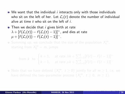
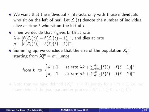
We want that the individual i interacts only with those individualswho sit on the left of her. Let Li (t) denote the number of individualalive at time t who sit on the left of i .
Then we decide that i gives birth at rateλ+ [f (Li (t))− f (Li (t)− 1)]+, and dies at rateµ+ [f (Li (t))− f (Li (t)− 1)]−.
Summing up, we conclude that the size of the population Xmt ,
starting from Xm0 = m, jumps
from k to
{k + 1, at rate λk +
∑k`=1[f (`)− f (`− 1)]+
k − 1, at rate µk +∑k
`=1[f (`)− f (`− 1)]−
Note that we have defined {Xmt , t ≥ 0} jointly for all m ≥ 1, i.e. we
have defined the two–parameter process {Xmt , t ≥ 0, m ≥ 1}.
Etienne Pardoux (Aix-Marseille) MANEGE, 26 Nov 2013collaborations avec Mamadou Ba, Vi Le, Anton Wakolbinger 6
/ 29

In case f linear, we have a branching process, and for each t > 0,{Xm
t , m ≥ 1} has independent increments.In the general case, we don’t expect that for fixed t, {Xm
t , m ≥ 1} isa Markov chain.However, {Xm
t , t ≥ 0}m≥1 is a path–valued Markov chain. We canspecify the transitions as follows.For 1 ≤ m < n, the law of {X n
t − Xmt , t ≥ 0}, given
{X `t , t ≥ 0, 1 ≤ ` ≤ m} and given that Xm
t = x(t), t ≥ 0, is that ofthe time–inhomogeneous jump Markov process whose rate matrix{Qk,`(t), k , ` ∈ Z+} satisfies
Q0,` = 0, ∀` ≥ 1 and for any k ≥ 1,
Qk,k+1(t) = λk +k∑`=1
[f (x(t) + `)− f (x(t) + `− 1)]+
Qk,k−1(t) = µk +k∑`=1
[f (x(t) + `)− f (x(t) + `− 1)]−
Qk,` = 0, if ` 6∈ {k − 1, k , k + 1}.Etienne Pardoux (Aix-Marseille) MANEGE, 26 Nov 2013
collaborations avec Mamadou Ba, Vi Le, Anton Wakolbinger 7/ 29

Exploration process of the forest of genealogical trees
D
B
Etienne Pardoux (Aix-Marseille) MANEGE, 26 Nov 2013collaborations avec Mamadou Ba, Vi Le, Anton Wakolbinger 8
/ 29

Call {Hms , s ≥ 0} the zigzag curve in the above picture (with slope
±2), and define the local time accumulated by Hm at level t up totime s by
Lms (t) = lim
ε→0
1
ε
∫ s
01t≤Hm
r <t+εdr .
Hm is piecewise linear, with slopes ±1. While the slope is 2, the rateof appearance of a maximum is
µ+ [f (bLms (Hm
s )c+ 1)− f (bLms (Hm
s )c)]− ,
and the rate of appearance of a minimum while the slope is −2 is
λ+ [f (bLms (Hm
s )c+ 1)− f (bLms (Hm
s )c)]+ .
Let Sm = inf{s > 0, Lms (0) ≥ m} the time needed for Hm
s to explorethe genealogical trees of m ancestors. If we assume that thepopulation goes extinct in finite time, we have the Ray–Knight typeresult (see next figure)
{Xmt , t ≥ 0, m ≥ 1} ≡ {Lm
Sm(t), t ≥ 0,m ≥ 1}.
Etienne Pardoux (Aix-Marseille) MANEGE, 26 Nov 2013collaborations avec Mamadou Ba, Vi Le, Anton Wakolbinger 9
/ 29

How to recover Xm from Hm ?
0 1 2 3
tlevel t
exploration time s S1
H1s
L1S1(t)
����������AAAAA����������AAAA������AAAAAAAAAAAAAA����AAAAAA
Etienne Pardoux (Aix-Marseille) MANEGE, 26 Nov 2013collaborations avec Mamadou Ba, Vi Le, Anton Wakolbinger 10
/ 29

Renormalization
Let N ≥ 1. Suppose that for some x > 0, m = bNxc, λ = 2N,
µ = 2N, replace f by fN = Nf (·/N). We define ZN,xt = N−1X
bNxct .
We have
Theorem
As N →∞,
{ZN,xt , t ≥ 0, x ≥ 0} ⇒ {Z x
t , t ≥ 0, x ≥ 0}
in D([0,∞); D([0,∞);R+)) equipped with the Skorohod topology of thespace of calag functions of x, with values in the Polish spaceD([0,∞);R+), equipped with the adequate metric.
{Z xt , t ≥ 0, x ≥ 0} solves for each x > 0 the Dawson–Li type SDE
Z xt = x +
∫ t
0f (Z x
s )ds + 2
∫ t
0
∫ Z xs
0W (ds, du),
where W (ds, du) is a space–time white noise.Etienne Pardoux (Aix-Marseille) MANEGE, 26 Nov 2013
collaborations avec Mamadou Ba, Vi Le, Anton Wakolbinger 11/ 29

How to check tightness ?
Our assumptions on f are pretty minimal. In order to check tightnessfor x fixed, we establish the two bounds
supN≥1
sup0≤t≤T
E(
ZN,xt
)2<∞, sup
N≥1sup
0≤t≤TE(−∫ t
0ZN,xs f (ZN,x
s )ds
)<∞,
and exploit Aldous’ criterion.
Concerning the tightness “in the x direction”, we establish thefollowing bound : for any 0 ≤ x < y < z with y − x ≤ 1, z − y ≤ 1,
E
[sup
0≤t≤T|ZN,y
t − ZN,xt |2 × sup
0≤t≤T|ZN,z
t − ZN,yt |2
]≤ C |z − x |2.
Etienne Pardoux (Aix-Marseille) MANEGE, 26 Nov 2013collaborations avec Mamadou Ba, Vi Le, Anton Wakolbinger 12
/ 29

Continuous population models
Etienne Pardoux (Aix-Marseille) MANEGE, 26 Nov 2013collaborations avec Mamadou Ba, Vi Le, Anton Wakolbinger 13
/ 29
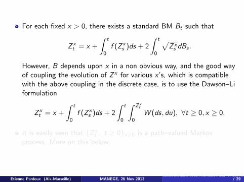
For each fixed x > 0, there exists a standard BM Bt such that
Z xt = x +
∫ t
0f (Z x
s )ds + 2
∫ t
0
√Z xs dBs .
However, B depends upon x in a non obvious way, and the good wayof coupling the evolution of Z x for various x ’s, which is compatiblewith the above coupling in the discrete case, is to use the Dawson–Liformulation
Z xt = x +
∫ t
0f (Z x
s )ds + 2
∫ t
0
∫ Z xs
0W (ds, du), ∀t ≥ 0, x ≥ 0.
It is easily seen that {Z xt , t ≥ 0}x≥0 is a path–valued Markov
process. More on this below.
Etienne Pardoux (Aix-Marseille) MANEGE, 26 Nov 2013collaborations avec Mamadou Ba, Vi Le, Anton Wakolbinger 14
/ 29

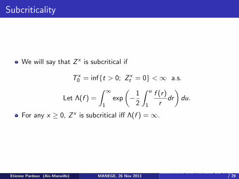
Subcriticality
We will say that Z x is subcritical if
T x0 = inf{t > 0; Z x
t = 0} <∞ a.s.
Let Λ(f ) =
∫ ∞1
exp
(−1
2
∫ u
1
f (r)
rdr
)du.
For any x ≥ 0, Z x is subcritical iff Λ(f ) =∞.
Etienne Pardoux (Aix-Marseille) MANEGE, 26 Nov 2013collaborations avec Mamadou Ba, Vi Le, Anton Wakolbinger 15
/ 29

A generalized Ray–Knight theorem
We assume now that f ∈ C 1(R+;R), and there exists a > 0 such thatf ′(x) ≤ a, for all x ≥ 0. Suppose that we are in the subcritical case.We consider the SDE
Hs = Bs +1
2
∫ s
0f ′(Lz
r (Hr ))dr +1
2Ls(0),
where Ls(0) denotes the local time accumulated by the process H atlevel 0 up to time s. We define Sx = inf{s > 0, Ls(0) > x}.We have
Theorem
The laws of the two random fields {LSx (t); t ≥ 0, x ≥ 0} and{Z x
t ; t ≥ 0, x ≥ 0} coincide.
The proof exploits ideas from Norris, Rogers, Williams (1987) whoprove the other Ray–Knight theorem in a similar context.
Etienne Pardoux (Aix-Marseille) MANEGE, 26 Nov 2013collaborations avec Mamadou Ba, Vi Le, Anton Wakolbinger 16
/ 29

Effect of the competition on the height and length of theforest of genealogical trees
Etienne Pardoux (Aix-Marseille) MANEGE, 26 Nov 2013collaborations avec Mamadou Ba, Vi Le, Anton Wakolbinger 17
/ 29

The finite population case
We assume again that f ∈ C (R+;R), f (0) = 0 and for some fixeda > 0, f (x + y)− f (x) ≤ ay , for all x , y ≥ 0. We assume in additionthat for some b > 0, f (x) < 0 for all x ≥ b. Define
Hm = inf{t > 0, Xmt = 0}, Lm =
∫ Hm
0 Xmt dt.
We have
Theorem
1 If∫∞b|f (x)|−1dx =∞, then supm Hm =∞ a.s.
2 If∫∞b|f (x)|−1dx <∞, then supm E(ecHm
) <∞ for some c > 0.
We have
Theorem
Assume in addition that g(x) = f (x)/x satisfies g(x + y)− g(x) ≤ ay.
1 If∫∞b|f (x)|−1xdx =∞, then supm Lm =∞ a.s.
2 If∫∞b|f (x)|−1xdx <∞, then supm E(ecLm
) <∞ for some c > 0.
Etienne Pardoux (Aix-Marseille) MANEGE, 26 Nov 2013collaborations avec Mamadou Ba, Vi Le, Anton Wakolbinger 18
/ 29

The case of continuous state space
Same assumptions as in the discrete case. We defineT x = inf{t > 0, Z x
t = 0}, Sx =∫ T x
0 Z xs ds.
We have
Theorem
1 If∫∞b|f (x)|−1dx =∞, then supx>0 T x =∞ a.s.
2 If∫∞b|f (x)|−1dx <∞, then supx>0 E(ecT x
) <∞ for some c > 0.
We have
Theorem
Assume in addition that g(x) = f (x)/x satisfies g(x + y)− g(x) ≤ ay.
1 If∫∞b|f (x)|−1xdx =∞, then supx Sx =∞ a.s.
2 If∫∞b|f (x)|−1xdx <∞, then supx E(ecSx
) <∞ for some c > 0.
Etienne Pardoux (Aix-Marseille) MANEGE, 26 Nov 2013collaborations avec Mamadou Ba, Vi Le, Anton Wakolbinger 19
/ 29

Intuitive idea
The reason why the above works is essentially because, ifg : R+ → R+ satifies ∫ ∞
0
1
g(x)dx <∞
then the solution of the ODE
x(t) = g(x), x(0) = x > 0
explodes in finite time.
Similarly the ODE
x(t) = −g(x), x(0) = +∞
has a solution which lives in C (R+;R+).
And the same is true for certain SDEs.
Etienne Pardoux (Aix-Marseille) MANEGE, 26 Nov 2013collaborations avec Mamadou Ba, Vi Le, Anton Wakolbinger 20
/ 29

The path–valued Markov process
Etienne Pardoux (Aix-Marseille) MANEGE, 26 Nov 2013collaborations avec Mamadou Ba, Vi Le, Anton Wakolbinger 21
/ 29

Restriction of our general model
For the rest of this talk, we restrict ourselves to the casef (x) = −γx2, with γ > 0. We will only consider the continuousstate–space case.
This means that we consider the solution Z xt of the SDE
Z xt = x − γ
∫ t
0(Z x
s )2ds + 2
∫ t
0
∫ Z xs
0W (ds, du).
Let us associate to this the solution of the same SDE with γ = 0,that is the critical Feller branching diffusion
Y xt = x + 2
∫ t
0
∫ Y xs
0W (ds, du).
If we consider those two SDEs with the same W , we obtain acoupling of Y and Z which satisfies Z x
t ≤ Y xt a.s. for all t ≥ 0, x ≥ 0.
Etienne Pardoux (Aix-Marseille) MANEGE, 26 Nov 2013collaborations avec Mamadou Ba, Vi Le, Anton Wakolbinger 22
/ 29

A better coupling
For each k, n ≥ 1, let xkn = k2−n, and Y n,k
t = Yxknt . For each n ≥ 1,
we now define recursively {Zn,kt , t ≥ 0} for k = 1, 2, . . ..
We set Zn,0t ≡ 0 and define Zn,1
t to be the solution of the SDE
Zn,1t = 2−n + θ
∫ t
0Zn,1s ds − γ
∫ t
0(Zn,1
s )2ds + 2
∫ t
0
∫ Zn,1s
0W (ds, du).
And for k ≥ 2, we let Zn,kt = Zn,1
t + V n,2t + · · ·+ V n,k
t , where
V n,kt = 2−n + θ
∫ t
0V n,ks ds − γ
∫ t
0
[2Zn,k−1
s V n,ks + (V n,k
s )2]
ds
+ 2
∫ t
0
∫ Y n,k−1s +V n,k
s
Y n,k−1s
W (ds, du).
Etienne Pardoux (Aix-Marseille) MANEGE, 26 Nov 2013collaborations avec Mamadou Ba, Vi Le, Anton Wakolbinger 23
/ 29

It is plain that for all k ≥ 1,
Zn,kt − Zn,k−1
t = V n,kt ≤ Y n,k
t − Y n,k−1t a.s. for all t ≥ 0,
and that the law of {Zn,kt , k ≥ 1, t ≥ 0} is the right one.
Recall that for each t > 0, x → Y xt has finitely many jumps on any
compact interval, and is constant between its jumps, and if 0 < s < t,
{x , Y xt 6= Y x−
t } ⊂ {x , Y xs 6= Y x−
s }.
The above construction allows to show that the same is true for aproperly defined {Z x
t , t ≥ 0, x > 0}, and moreover for all t > 0,
{x , Z xt 6= Z x−
t } ⊂ {x , Y xt 6= Y x−
t }.
Consequently, as Y x , Z x is a sum of jumps.
Etienne Pardoux (Aix-Marseille) MANEGE, 26 Nov 2013collaborations avec Mamadou Ba, Vi Le, Anton Wakolbinger 24
/ 29

More precisely, we can write Y x as the solution of the SDE (E stands forthe space of excursions away from 0)
Y x· =
∫[0,x]×E
uN(dy , du),
where N is a Poisson random measure on R+ × E with mean measuredy ×Q(du), where Q is the excursion measure of the Feller diffusion.
Etienne Pardoux (Aix-Marseille) MANEGE, 26 Nov 2013collaborations avec Mamadou Ba, Vi Le, Anton Wakolbinger 25
/ 29

We have similarly that x → Z x is a sum of excursions. Call N(dy , du)the corresponding point process, which is such that for all x > 0,
Z x =
∫[0,x]×E
uN(dy , du).
The predictable intensity of N is
L(Z y , u)Q(du)dy ,
where (with ζ = inf{t, Ut = 0} the lifetime of U)
L(Z ,U) = exp
(−γ
4
∫ ζ
0(2Zt + Ut)dUt −
γ2
8
∫ ζ
0(2Zt + Ut)
2Utdt
).
This follows readily from the statement
Z x =
∫[0,x]×E
L(Z y , u)uQ(du)dy + Mx ,
where Mx is an E –valued Fx–martingale.
Etienne Pardoux (Aix-Marseille) MANEGE, 26 Nov 2013collaborations avec Mamadou Ba, Vi Le, Anton Wakolbinger 26
/ 29

The last identity is proved as follows. We want to establish that forany t > 0,
Z x(t) =
∫[0,x]×E
Lγ(Z y , u)u(t)Q(du)dy + Mx(t).
Clearly if x is a dyadic number, then for n large enough
Z x(t) =x2n∑k=1
2−nE(
Z xk+1 − Z xk∣∣∣Z xk
)+ Mx
n (t),
where {Mxn (t), x > 0} is a martingale.
Now
E(
Z x+y (t)− Z x(t)∣∣∣Z x)
= E(
Lγ(Z x ,Uy )Uyt
∣∣∣Z x),
where
Uyt = y + 2
∫ t
0
√UsdBs .
Etienne Pardoux (Aix-Marseille) MANEGE, 26 Nov 2013collaborations avec Mamadou Ba, Vi Le, Anton Wakolbinger 27
/ 29

But
y−1E(
Lγ(Z x ,Uy )Uyt
∣∣∣Z x)
= EQy,t
(Lγ(Z x ,Uy )
∣∣∣Z x),
where under Qy ,t
Ur = y + 4t ∧ r + 2
∫ t
0
√UsdBs .
Finally we can take the limit as y → 0 in the last identity, yielding
y−1E(
Lγ(Z x ,Uy )Uyt
∣∣∣Z x)→ EQ0,t
(Lγ(Z x ,U)
∣∣∣Z x).
It just remain to verify that
EQ0,t
(Lγ(Z x ,U)
∣∣∣Z x)
=
∫E
Lγ(Z x , u)u(t)Q(du),
where Q is the above excursion measure.
Etienne Pardoux (Aix-Marseille) MANEGE, 26 Nov 2013collaborations avec Mamadou Ba, Vi Le, Anton Wakolbinger 28
/ 29

Bibliography
E. Pardoux, A. Wakolbinger, From Brownian motion with a local timedrift to Feller’s branching diffusion with logistic growth, Elec. Comm.in Probab. 16, 720–731, 2011.
V. Le, E. Pardoux, A. Wakolbinger, Trees under attack : aRay–Knight representation of Feller’s branching diffusion with logisticgrowth, Probab. Theory & Rel. Fields 155 583–619, 2013.
M. Ba, E. Pardoux, Branching processes with competition andgenralized Ray–Knight theorem, submitted, 2013.
V. Le, E. Pardoux, Height and the total mass of the forest ofgenealogical trees of a large population with general competition,ESAIM P & S, 2013, to appear.
J.R. Norris, L.C.G. Rogers, D. Williams, Self–avoiding random walks:a Brownian motion model with local time drift, Probab. Theory &Rel. Fields 74, 271–287, 1987.
J. Pitman, M. Yor, A decomposition of Bessel bridges, Z. furWahrscheinlichkeitstheorie verw. Gebiete 59, 425–457, 1982.
Etienne Pardoux (Aix-Marseille) MANEGE, 26 Nov 2013collaborations avec Mamadou Ba, Vi Le, Anton Wakolbinger 29
/ 29


![[Start] Generate random population of N chromosomes (suitable solutions for the problem)](https://img.pdfslide.net/doc/110x75/56816945550346895de0ce80/start-generate-random-population-of-n-chromosomes-suitable-solutions-for.jpg)