RANDOM GRAPHS: DYNAMICAL PROCESSES AND REPLICA …

2

RANDOM GRAPHS: DYNAMICAL PROCESSES ANDREPLICA METHOD

2.1 The solution space of random 3-XORSAT

2.1.1 Numerical simulations for the threshold

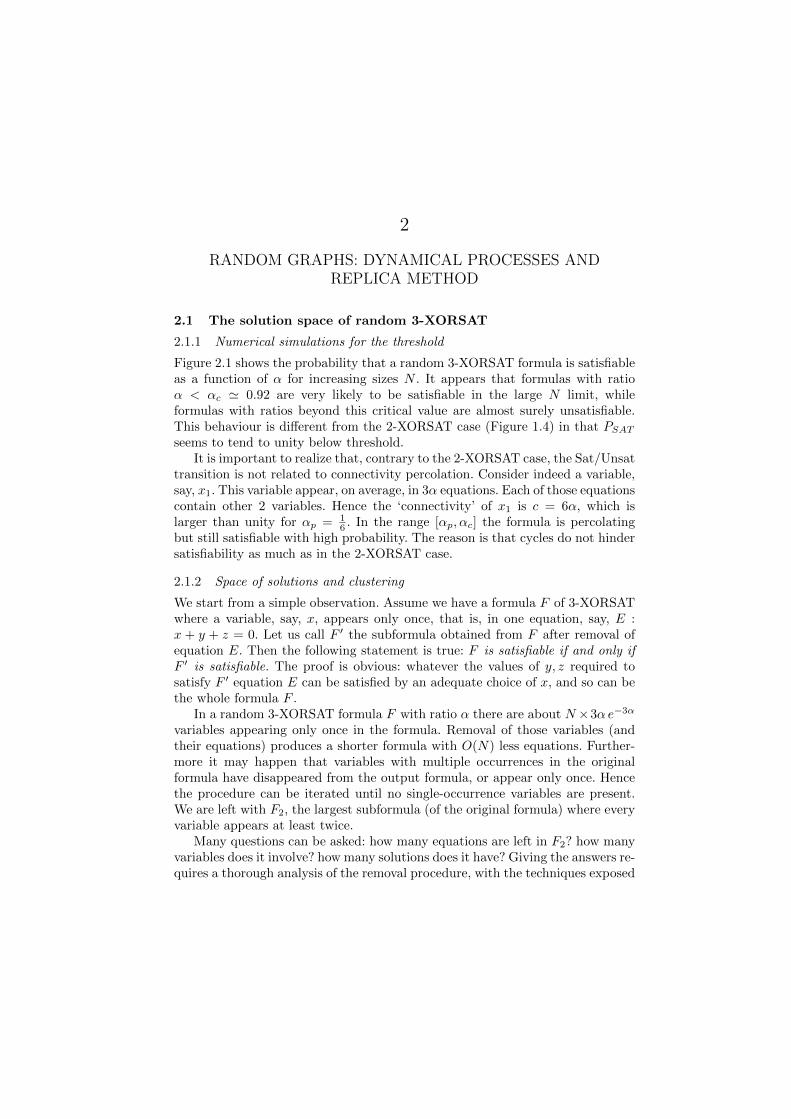
Figure 2.1 shows the probability that a random 3-XORSAT formula is satisfiableas a function of α for increasing sizes N . It appears that formulas with ratioα < αc 0.92 are very likely to be satisfiable in the large N limit, whileformulas with ratios beyond this critical value are almost surely unsatisfiable.This behaviour is different from the 2-XORSAT case (Figure 1.4) in that PSAT

seems to tend to unity below threshold.It is important to realize that, contrary to the 2-XORSAT case, the Sat/Unsat

transition is not related to connectivity percolation. Consider indeed a variable,say, x1. This variable appear, on average, in 3α equations. Each of those equationscontain other 2 variables. Hence the ‘connectivity’ of x1 is c = 6α, which islarger than unity for αp = 1

6 . In the range [αp,αc] the formula is percolatingbut still satisfiable with high probability. The reason is that cycles do not hindersatisfiability as much as in the 2-XORSAT case.

2.1.2 Space of solutions and clustering

We start from a simple observation. Assume we have a formula F of 3-XORSATwhere a variable, say, x, appears only once, that is, in one equation, say, E :x + y + z = 0. Let us call F the subformula obtained from F after removal ofequation E. Then the following statement is true: F is satisfiable if and only ifF is satisfiable. The proof is obvious: whatever the values of y, z required tosatisfy F equation E can be satisfied by an adequate choice of x, and so can bethe whole formula F .

In a random 3-XORSAT formula F with ratio α there are about N×3α e−3α

variables appearing only once in the formula. Removal of those variables (andtheir equations) produces a shorter formula with O(N) less equations. Further-more it may happen that variables with multiple occurrences in the originalformula have disappeared from the output formula, or appear only once. Hencethe procedure can be iterated until no single-occurrence variables are present.We are left with F2, the largest subformula (of the original formula) where everyvariable appears at least twice.

Many questions can be asked: how many equations are left in F2? how manyvariables does it involve? how many solutions does it have? Giving the answers re-quires a thorough analysis of the removal procedure, with the techniques exposed

THE SOLUTION SPACE OF RANDOM 3-XORSAT 25

0,6 0,8 1 1,2

α

0

0,2

0,4

0,6

0,8

1

Pro

b. S

AT

3-XORSAT

50

100

200

P=0.9

P=0.1800

Fig. 2.1. Probability that a random 3-XORSAT formula is satisfiable as a func-tion of the ratio α of equations per variable, and for various sizes N . Thedotted line locates the threshold αc 0.918.

in the next Section. The outcome depends on the value of the ratio compared to

αd = minb

− log(1− b)

3 b2 0.8184 . . . (2.1)

hereafter called clustering threshold. With high probability when N → ∞ F2 isempty if α < αd, and contains an extensive number of equations, variables whenα > αd. In the latter case calculation of the first and second moments of thenumber of solutions of F2 shows that this number does not fluctuate around thevalue eN sclu(α)+o(N) where

sclu(α) = (b− 3α b2 + 2α b3) ln 2 (2.2)

and b is the strictly positive solution of the self-consistent equation

1− b = e−3α b2

. (2.3)

Hence F2 is satisfiable if and only if α < αc defined through sclu(αc) = 0, thatis,

αc 0.9179 . . . . (2.4)

This value is, by virtue of the equivalence between F and F2 the Sat/Unsatthreshold for 3-XORSAT, in excellent agreement with Figure 2.1.

How can we reconstruct the solutions of F from the ones of F2? The pro-cedure is simple. Start from one solution of F2 (empty string if α < αd). Then

26 RANDOM GRAPHS: DYNAMICAL PROCESSES AND REPLICA METHOD

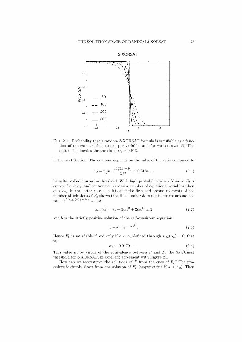
Fig. 2.2. Graph representation of the 3-XORSAT formula. Vertices (variables)are joined by plaquettes (values 0, 1 of second members are not shown here).A step of decimation consists in listing all 1-variables (appearing only once inthe formula, shown by gray vertices), choosing randomly one of them (grayvertex pointed by the arrow), and eliminating this variable and its plaquette.New 1-variables may appear. Decimation is repeated until no 1-variable isleft.

introduce back the last equation which was removed since it contained n ≥ 1single-occurrence variable. If n = 1 we fix the value of this variable in a uniqueway. If n = 2 (respectively n = 3) there are 2 (respectively, 4) ways of assigningthe reintroduced variables, defining as many solutions from our initial, partialsolution. Reintroduction of equations one after the other according to the Last In– First Out order gives us more and more solutions from the initial one, until weget a bunch of solutions of the original formula F . It turns out that the numberof solutions created this way is eN sin(α)+o(N) where

sin(α) = (1− α) ln 2− scluster(α) . (2.5)

The above formula is true for α > αd, and should be intended as sin(α) =(1− α) ln 2 for α < αd. These two entropies are shown in Figure 2.3. The totalentropy, s∗(α) = sin(α) + sclu(α), is simply (1 − α) ln 2 for all ratios smallerthan the Sat/Unsat threshold. It shows no singularity at the clustering threshold.However a drastic change in the structure of the space of solutions takes place,symbolized in the phase diagram of Figure 2.4:

• For ratios α < αd the intensive Hamming distance between two solu-tions is, with high probability, equal to d = 1/2. Solutions thus differ onN/2 + o(N) variables, as if they were statistically unrelated assignmentsof the N Boolean variables. In addition the space of solutions enjoys someconnectedness property. Any two solutions are connected by a path (in thespace of solutions) along which successive solutions differ by a boundednumber of variables. Losely speaking one is not forced to cross a big regionprived of solutions when going from one solution to another.

• For ratios α > αd the space of solutions is not connected any longer.

ANALYSIS OF THE DECIMATION DYNAMICAL PROCESS 27

0 0,5 1

ratio α

0

0,5

1

Entr

opie

s of so

lutio

ns

and c

lust

ers

s

sclu

αc

αd

sin

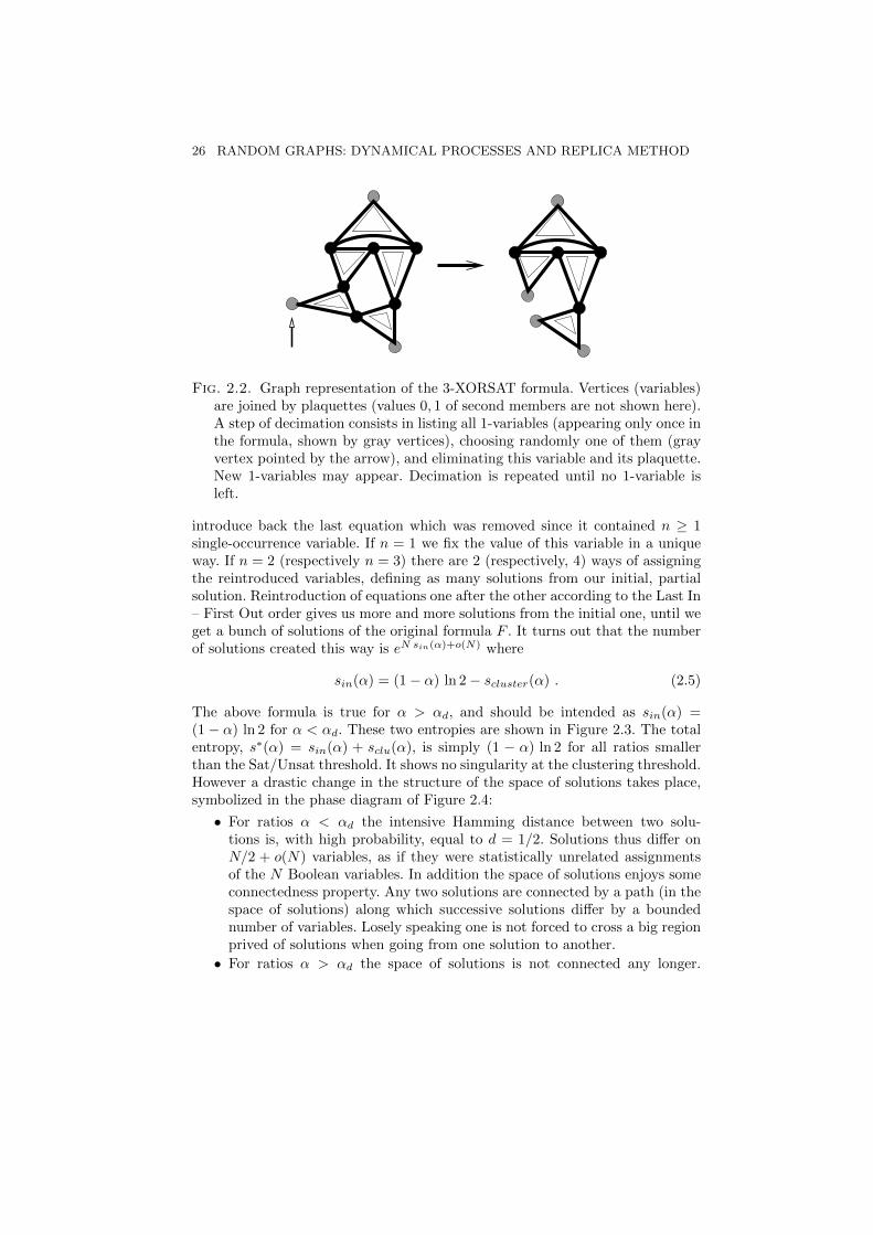
Fig. 2.3. Entropies (base 2 logarithms divided by size N) of the numbers ofsolutions and clusters as a function of the ratio α. The entropy of solutionsequals 1−α for α < αc 0.918. For α < αd 0.818, solutions are uniformlyscattered on the N -dimensional hypercube. At αd the solution space discon-tinuously breaks into disjoint clusters. The entropies of clusters, scluster, andof solutions in each cluster, sin, are such that scluster + sin = s. At αc thenumber of clusters stops being exponentially large (scluster = 0). Above αc

there is almost surely no solution.

It is made of an exponentially large (in N) number Nclu = eN scluster

of connected components, called clusters, each containing an exponentiallylarge numberNin = eN sin of solutions. Two solutions belonging to differentclusters lie apart at a Hamming distance dclu = 1/2 while, inside a cluster,the distance is din < dclu. b given by (2.3) is the fraction of variables havingthe same value in all the solutions of a cluster (defined as the backbone).

We present in Section 2.3 the statistical physics tools developed to deal withthe scenario of Figure 2.4.

2.2 Analysis of the decimation dynamical process

We now sketch how the above results may found back rigorously. The techniquesused are borrowed from probability theory, and the analysis of algorithms. Letus call -variable a variable which appears in distinct equations (plaquettes, seeFigure 2.2) of the 3-XORSAT formula. Plaquettes containing at least a 1-variableare never frustrated. Our decimation procedure consists in a recursive eliminationof these plaquettes and attached 1-variables, until no 1-variable is left. We definethe numbers N(T ) of –variables after T steps of the decimation algorithm, i.e.once T plaquettes have been removed, and their set N (T ) = N(T ), ≥ 0. Thevariations of the Ns during the (T + 1)th step of the algorithm are stochastic


0

satisfiable unsatisfiable

d

d

d

in

clu

αd

αc

α

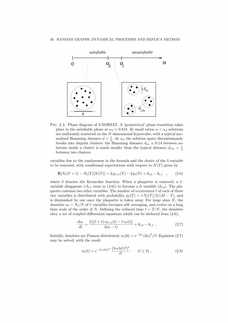
Fig. 2.4. Phase diagram of 3-XORSAT. A ‘geometrical’ phase transition takesplace in the satisfiable phase at αd 0.818. At small ratios α < αd solutionsare uniformely scattered on the N -dimensional hypercube, with a typical nor-malized Hamming distance d = 1

2 . At αd the solution space discontinuouslybreaks into disjoint clusters: the Hamming distance din 0.14 between so-lutions inside a cluster is much smaller than the typical distance dclu = 1

2between two clusters.

variables due to the randomness in the formula and the choice of the 1-variableto be removed, with conditional expectations with respect to N (T ) given by

E[N(T + 1)−N(T )|N (T )] = 2 p+1(T )− 2 p(T ) + δ,0 − δ,1 , (2.6)

where δ denotes the Kronecker function. When a plaquette is removed, a 1-variable disappears (-δ,1 term in (2.6)) to become a 0–variable (δ,0). The pla-quette contains two other variables. The number of occurrences of each of thesetwo variables is distributed with probability p(T ) = N(T )/3/(M − T ), andis diminished by one once the plaquette is taken away. For large sizes N , thedensities n = N/N of –variables becomes self–averaging, and evolve on a longtime scale of the order of N . Defining the reduced time t = T/N , the densitiesobey a set of coupled differential equations which can be deduced from (2.6),

dn

dt=

2 [(+ 1)n+1(t)− n(t)]

3(α− t)+ δ,0 − δ,1 . (2.7)

Initially, densities are Poisson distributed: n(0) = e−3α (3α)/!. Equation (2.7)may be solved, with the result

n(t) = e−3α b(t)2 (3α b(t)2)

!( ≥ 2) , (2.8)

ANALYSIS OF THE DECIMATION DYNAMICAL PROCESS 29

0 0.2 0.4 0.6 0.8 1

Reduced time t/α

0

0.1

0.2

De

nsi

ty o

f 1

-va

ria

ble

s n

1

α=0.818α=0.9

α αd c

0.7 0.8 0.9α

0

0.5

1

α’

α=0.7

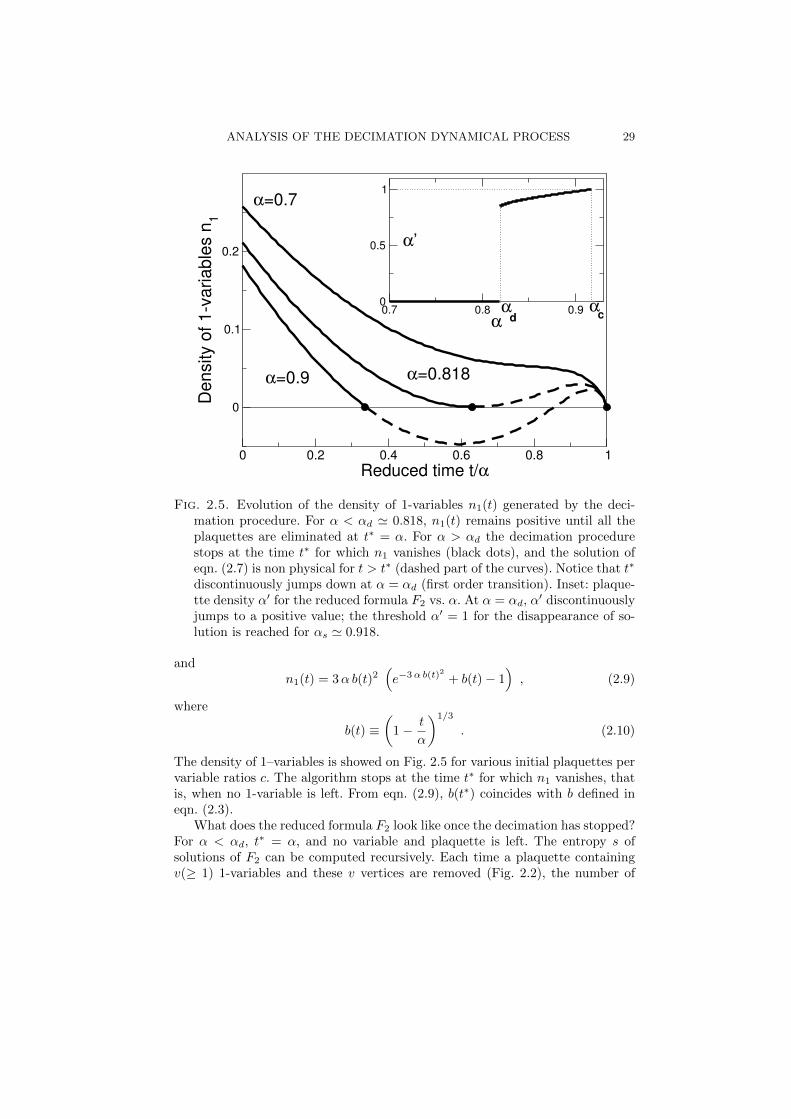
Fig. 2.5. Evolution of the density of 1-variables n1(t) generated by the deci-mation procedure. For α < αd 0.818, n1(t) remains positive until all theplaquettes are eliminated at t∗ = α. For α > αd the decimation procedurestops at the time t∗ for which n1 vanishes (black dots), and the solution ofeqn. (2.7) is non physical for t > t∗ (dashed part of the curves). Notice that t∗

discontinuously jumps down at α = αd (first order transition). Inset: plaque-tte density α for the reduced formula F2 vs. α. At α = αd, α discontinuouslyjumps to a positive value; the threshold α = 1 for the disappearance of so-lution is reached for αs 0.918.

andn1(t) = 3α b(t)2

e−3α b(t)2 + b(t)− 1

, (2.9)

where

b(t) ≡1− t

α

1/3

. (2.10)

The density of 1–variables is showed on Fig. 2.5 for various initial plaquettes pervariable ratios c. The algorithm stops at the time t∗ for which n1 vanishes, thatis, when no 1-variable is left. From eqn. (2.9), b(t∗) coincides with b defined ineqn. (2.3).

What does the reduced formula F2 look like once the decimation has stopped?For α < αd, t∗ = α, and no variable and plaquette is left. The entropy s ofsolutions of F2 can be computed recursively. Each time a plaquette containingv(≥ 1) 1-variables and these v vertices are removed (Fig. 2.2), the number of


solutions gets divided by 2v−1, and the average entropy (base 2 logarithm) ofsolutions decreased by E[v − 1|N (T )] = 2 p1(T ). As no variable is left when thealgorithm stops, the final value for the entropy vanishes, giving

s =

t∗

0dt

2n1(t)

3 (α− t)+ e−3c , (2.11)

where the last term comes from the contribution n0(0) of 0-variables. Using eqn.(2.9) and t∗ = c, we find back s = 1− α.

When αd < α < αc, the decimation procedure stops at t∗ < α, and has notsucceeded in eliminating all plaquettes and variables. The remaining fraction ofplaquettes per variable, α = (α − t∗)/σ where σ =

≥2 n(t∗), is plotted as a

function of α in the Inset of Fig. 2.5. Each solution of F2 can be seen as a ‘seed’from which a cluster of solution of F in the original configuration space can bereconstructed. To do so, plaquettes which were eliminated during decimation arereintroduced, one after the other, and the variables they contain are assigned allpossible values that leave the plaquettes unfrustrated. Combining any of thesepartial variable assignments with (free) 0-variables assignments, all the solutionsin a cluster are obtained. Repeating the argument leading to the calculation ofthe entropy in the α < αd case, we find that the average entropy sin of solutionsin a cluster is given by the r.h.s. of eqn. (2.11).

To complete the description of clusters, some statistical knowledge abouttheir seeds is required. The average value of the number U of solutions of F2

can be easily computed: U = 2N(1−α

). As the average number of solutionsis an upper bound to the probability of existence of at least one solution weconclude that U almost surely vanishes when α > 1. The calculation of thesecond moment is harder and will not be done here. The result is that U showweak fluctuations around its average value. Hence the entropy of solutions is,with high probability, given by 1

NlogU = N

N(1 − α) log 2. This entropy is

precisely the logarithm of the number of clusters sclu defined above. In additionwe obtain the value of the threshold αc through the condition α(αc) = 1.

The reconstruction process allows a complete characterization of solutions,in terms of an extensive number of (possibly overlapping) blocks made of fewvariables, each block being allowed to flip as a whole from a solutions to another.When α < αd, with high probability, two randomly picked solutions differ overa fraction d = 1/2 of variables, but are connected through a sequence of O(N)successive solutions differing over O(1) variables only. For αd < α < αc, flip-pable blocks are juxtaposed to a set of seed-dependent frozen variables. To provethe existence of clustering (Fig. 2.4), one can check that the largest Hammingdistance dmax

1 between two solutions associated to the same seed is lower thanthe smallest possible distance dmin

0 between solutions reconstructed from twodifferent seeds.

THE REPLICA METHOD 31

2.3 The replica method

2.3.1 From moments to large deviations for the entropy

Let us define the intensive entropy s through N = eN s. As N is random (atfixed α, N) so is s. We assume that the distribution of s can be described, in thelarge size limit, by a rate function ω(s) (which depends on α). Hence,

N q =

ds e−N ω(s) ×eN s

q ∼ expN max

s

q s− ω(s)

(2.12)

using the Laplace method. If we are able to estimate the leading behaviour ofthe qth moment of the number of solutions when N gets large at fixed α,

N q ∼ eN g(q) , (2.13)

then ω can be easily calculated by taking the Legendre transform of g. In par-ticular the typical entropy is obtained by s∗ = dg

dq(q → 0). This is the road we

will follow below. We will show how g(q) can be calculated when q takes integervalues, and then perform an analytic continuation to non integer q. The con-tinuation leads to substantial mathematical difficulties, but is not uncommonin statistical physics e.g. the q → 1 limit of the q-state Potts model to recoverpercolation, or the n → 0 limit of the O(n) model to describe self-avoiding walks.

To calculate the qth moment we will have to average over the random compo-nents of formulas F , that is, the K-uplets of index variables in the first membersand the v = 0, 1 second members. Consider now homogeneous formulas Fh whosefirst members are randomly drawn in the same way as for F , but with all secondmembers v = 0. The number Nh of solutions of a homogeneous formula is alwayslarger or equal to one. It is a simple exercise to show that

N q+1 = 2N(1−α) × Nh

q , (2.14)

valid for any positive integer q14. Therefore it is sufficient to calculate the mo-ments of Nh = eN gh(q) since (2.14) gives a simple identity between g(q+ 1) andgh(q).

2.3.2 Free energy for replicated variables

The qth power of the number of solutions to a homogeneous system reads

Nh

q=

X

M

=1

e(X)

q

=

X1,X2,...,Xq

M

=1

q

a=1

e(Xa) , (2.15)

where e(X) is 1 if equation is satisfied by assignment X, and 0 otherwise.The last sum runs over q assignments Xa, with a = 1, 2, . . . , q of the Boolean

14Actually the identity holds for q = 0 too, and is known under the name of harmonic meanformula.


variables, called replicas of the original assignment X. It will turn useful todenote by xi = (x1

i, x2

i, . . . , xq

i) the q-dimensional vector whose components are

the values of variable xi in the q replicas. To simplify notations we considerthe case K = 3 only here, but extension to other values of K is straightforward.Averaging over the instance, that is, the triplets of integers labelling the variablesinvolved in each equation , leads to the following expression for the qth moment,

Nh

q =

X1,X2,...,Xq

q

a=1

e(Xa)M

=

X1,X2,...,Xq

1

N3

1≤i,j,k≤N

δxi+xj+xk +O

1

N

M

(2.16)

where δx = 1 if the compoments of x are all null mod. 2, and 0 otherwise. Wenow procede to some formal manipulations of the above equation (2.16).

First step. Be X = X1, X2, . . . , Xq one of the 2 qN replica assignment.Focus on variable i, and its attached assignment vector, xi. The latter may beany of the 2q possible vectors e.g. xi = (1, 0, 1, 0, 0, . . . , 0) if variable xi is equalto 0 in all but the first and third replicas. The histogram of the assignmentsvectors given replica assignment X ,

ρx|X

=

1

N

N

i=1

δx−xi , (2.17)

counts the fraction of assignments vectors xi having value x when i scans thewhole set of variables from 1 to N . Of course, this histogram is normalised tounity,

x

ρx= 1 , (2.18)

where the sum runs over all 2q assignment vectors. An simple but essentialobservation is that the r.h.s. of (2.16) may be rewritten in terms of the abovehistogram,

1

N3

1≤i,j,k≤N

δxi+xj+xk =

x,x

ρxρx ρ

x+ x . (2.19)

Keep in mind that ρ in (2.17,2.19) depends on the replica assignement X underconsideration.

Second step. According to (2.19), two replica assignments X1 and X2 defin-ing the same histogram ρ will give equal contributions to

Nh

q. The sum overreplica assignments X can therefore be replaced over the sum over possible his-tograms provided the multiplicity M of the latter is taken properly into account.


This multiplicity is also equal to the number of combinations of N elements (thexi vectors) into 2q sets labelled by x and of cardinalities N ρ(x). We obtain

Nh

q =(norm)

ρ

e N Gh

ρ,α

+ o(N) , (2.20)

where the (norm) subscript indicates that the sum runs over histograms ρ nor-malized according to (2.18), and

Gh

ρ,α

= −

x

ρ(x) ln ρ(x) + α ln

x,x

ρxρx ρ

x+ x

. (2.21)

In the large N limit, the sum in (2.20) is dominated by the histogram ρ∗ maxi-mizing the functional Gh.

Third step. Maximisation of function Gh over normalized histograms canbe done within the Lagrange multiplier formalism. The procedure consists inconsidering the modified function

GLM

h

ρ,λ,α

= Gh

ρ,α

+ λ

1−

x

ρx

, (2.22)

and first maximise GLM

hwith respect to histograms ρ without caring about the

normalisation constraint, and then optimise the result with respect to λ. Wefollow this procedure with Gh given by (2.21). Requiring that GLM

hbe maximal

provides us with a set of 2q coupled equations for ρ∗,

ln ρ∗(x) + 1 + λ− 3 α

x

ρ∗x ρ∗

x+ x

x,x

ρ∗x ρ∗

x ρ∗

x + x = 0 , (2.23)

one for each assignment vector x. The optimisation equation over λ implies thatλ in (2.23) is such that ρ∗ is normalised. At this point of the above and ratherabstract calculation it may help to understand the interpretation of the optimalhistogram ρ∗.

2.3.3 The order parameter

Consider q solutions labelled by a = 1, 2, . . . , q of the same random and homoge-neous instance and a variable, say, xi. What is the probability, over instances andsolutions, that this variable takes, for instance, value 0 in the first and fourth so-lutions, and 1 in all other solutions? In other words, what is the probability that

the assignment vector xi = (x1i, x2

i, . . . , xq

i) is equal to x = (0, 1, 1, 0, 1, 1, . . . , 1)?

The answer is


p(x) =

1

(Nh)q

X1,X2,...,Xq

δxi−x

M

l=1

q

a=1

e(Xa)

(2.24)

where the dependence on i is wiped out by the average over the instance. Theabove probability is an interesting quantity; it provides us information aboutthe ‘microscopic’ nature of solutions. Setting q = 1 gives us the probabilitiesp(0), p(1) that a variable is false or true respectively, that is, takes the same valueas in the null assignment or not. For generic q we may think of two extremesituations:

• a flat p over assignment vectors, p(x) = 1/2q, corresponds to essentially

orthogonal solutions;• on the opposite, a concentrated probability e.g. p(x) = δx implies thatvariables are extremely constrained, and that the (almost) unique solutionis the null assignment.

The careful reader will have already guessed that our calculation of the qth

moment gives access to a weighted counterpart of p. The order parameter

ρ∗(x) =1

(Nh)q

X1,X2,...,Xq

δxi−x

M

l=1

q

a=1

e(Xa)

, (2.25)

is not equal to p even when q = q. However, at the price of mathematicalrigor, the exact probability p over vector assignments of integer length q can bereconstructed from the optimal histogram ρ∗ associated to moments of order qwhen q is real-valued and sent to 0. The underlying idea is the following. Consider(2.25) and an integer q < q. From any assignment vector x of length q, we definetwo assignment vectors x, x of respective lengths q, q−q corresponding to thefirst q and the last q−q components of x respectively. Summing (2.25) over the2q−q

assignment vectors x gives,

x

ρ∗(x, x) =1

(Nh)q

Xa

δxi−x

Nh

q−q

l,a

e(Xa)

. (2.26)

As q now appears in the powers of Nh in the numerator and denominator only,it can be formally send to zero at fixed q, yielding

limq→0

x

ρ∗(x, x) = p(x) (2.27)

from (2.24). This identity justifies the denomination order parameter given toρ∗.

Having understood the significance of ρ∗ helps us to find appropriate solutionsto (2.23). Intuitively and from the discussion of the first moment case q = 1,p is expected to reflect both the special role of the null assignment (which is


a solution to all homogeneous systems) and the ability of other solutions of arandom system to be essentially orthogonal to this special assignment. A possibleguess is thus

p(x) =1− b

2q+ b δx , (2.28)

where b expresses some degree of ‘correlation’ of solutions with the null one.Hypothesis (2.28) interpolates between the fully concentrated (b = 1) and flat(b = 0) probabilities. b measures the fraction of variables (among the N ones)that take the 0 values in all q solution, and coincides with the notion of backboneintroduced in Section 2.1.2. Hypothesis (2.28) is equivalent, from the connection(2.27) between p and the annealed histogram ρ∗ to the following guess for thesolution of the maximisation condition (2.23),

ρ∗(x) =1− b

2q+ b δx . (2.29)

Insertion of Ansatz (2.29) in (2.23) shows that it is indeed a solution provided bis shrewdly chosen as a function of q and α, b = b∗(q,α). Its value can be eitherfound from direct resolution of (2.23), or from insertion of histogram (2.29) inGh (2.21) and maximisation over b, with the result,

gh(q,α) = max0≤b≤1

Ah(b, q,α) (2.30)

where

Ah(b, q,α) = −1− 1

2q

(1− b) ln

1− b

2q

(2.31)

−b+

1− b

2q

ln

b+

1− b

2q

+ α ln

b3 +

1− b3

2q

,

where the maximum is precisely reached in b∗. Notice that, since ρ∗ in (2.29) isentirely known from the value of b∗, we shall indifferently call order parameterρ∗, or b∗ itself.

2.3.4 Results

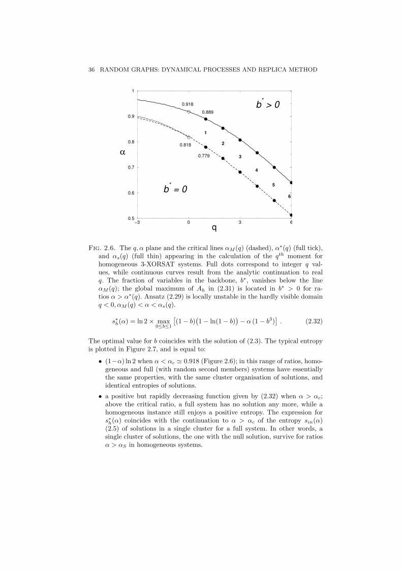
Numerical investigation of Ah (2.31) shows that: for α < αM (q) the only localmaximum of Ah is located in b∗ = 0, and Ah(q,α) = q(1−α) ln 2; when αM (q) <α < α∗(q), there exists another local maximum in b > 0 but the global maximumis still reached in b∗ = 0; when α > α∗(q), the global maximum is located inb∗ > 0. The αM and α∗ lines divide the q,α plane as shown in Figure 2.6.Notice that, while the black dots in Figure 2.6 correspond to integer-valued q,the continuous lines are the output of the implicit analytic continuation to realq done by the replica calculation.

Taking the derivative of (2.30) with respect to q and sending q → 0 we obtainthe typical entropy of a homogeneous 3-XORSAT system at ratio α,


−3 0 3 6

q0.5

0.6

0.7

0.8

0.9

1

α

1

2

3

4

5

0.889

0.779

0.918

6

0.818

b* = 0

b* > 0

Fig. 2.6. The q,α plane and the critical lines αM (q) (dashed), α∗(q) (full tick),and αs(q) (full thin) appearing in the calculation of the qth moment forhomogeneous 3-XORSAT systems. Full dots correspond to integer q val-ues, while continuous curves result from the analytic continuation to realq. The fraction of variables in the backbone, b∗, vanishes below the lineαM (q); the global maximum of Ah in (2.31) is located in b∗ > 0 for ra-tios α > α∗(q). Ansatz (2.29) is locally unstable in the hardly visible domainq < 0,αM (q) < α < αs(q).

s∗h(α) = ln 2× max

0≤b≤1

(1− b)

1− ln(1− b)

− α (1− b3)

. (2.32)

The optimal value for b coincides with the solution of (2.3). The typical entropyis plotted in Figure 2.7, and is equal to:

• (1−α) ln 2 when α < αc 0.918 (Figure 2.6); in this range of ratios, homo-geneous and full (with random second members) systems have essentiallythe same properties, with the same cluster organisation of solutions, andidentical entropies of solutions.

• a positive but rapidly decreasing function given by (2.32) when α > αc;above the critical ratio, a full system has no solution any more, while ahomogeneous instance still enjoys a positive entropy. The expression fors∗h(α) coincides with the continuation to α > αc of the entropy sin(α)

(2.5) of solutions in a single cluster for a full system. In other words, asingle cluster of solutions, the one with the null solution, survive for ratiosα > αS in homogeneous systems.


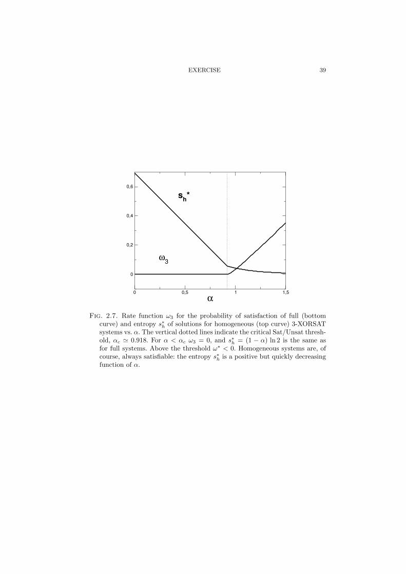
Atypical instances can be studied and the large deviation rate function forthe entropy can be derived from (2.30) for homogeneous systems, and usingequivalence (2.14), for full systems. Minimizing over the entropy we obtain therate function ω3(α) associated to the probability that a random 3-XORSATsystem is satisfiable, with the result shown in Figure 2.7. As expected we findω3 = 0 for α < αc and ω3 > 0 for α > αc, allowing us to locate the Sat/Unsatthreshold.

Notice that the emergence of clustering can be guessed from Figure 2.6. Itcoincides with the appearance of a local maximum of Ah (2.31) with a nonvanishing backbone b. While in the intermediate phase αd < α < αc, the height ofthe global maximum equals the total entropy s∗, the height of the local maximumcoincides with the entropy of clusters scluster (2.2).

2.3.5 Stability of the replica Ansatz

The above results rely on Ansatz (2.29). A necessary criterion for its validityis that ρ∗ locates a true local maximum of Gh , and not merely a saddle-point.Hence we have to calculate the Hessian matrix of Gh in ρ∗, and check that theeigenvalues are all negative [?]. Differentiating (2.21) with respect to ρ(x) andρ(x) we obtain the Hessian matrix

H(x, x) = − δx+x

ρ∗(x)+ 6α

ρ∗(x+ x)

D− 9α

N(x)

D

N(x)

D, (2.33)

where D = 1−b3

2q + b3, N(x) = 1−b2

2q + b2 δx. We use b instead of b∗ to ligthen thenotations, but it is intended that b is the backbone value which maximizes Ah

(2.31) at fixed q,α. To take into account the global constraint over the histogram(2.18) one can express one fraction, say, ρ(0), as a function of the other fractionsρ(x), x = 0. GH is now a fonction of 2q−1 independent variables, with a Hessianmatrix H simply related to H,

H(x, x) = H(x, x)−H(x,0)−H(0, x) +H(0,0) . (2.34)

Plugging expression (2.33) into (2.34) we obtain

H(x, x) = λR δx+x +1

2q − 1

λL − λR) where

λR = 6αb

D− 2q

1− b(2.35)

λL = 2q6α

b

D− 2q

(1− b)(1− b+ 2qb)− 9α(1− 2−q)

b4

D2

.

Diagonalization of H is immediate, and we find two eigenvalues:

• λL (non degenerate). The eigenmode corresponds to a uniform infinitesimalvariation of ρ(x) for all x = 0, that is, a change of b in (2.29). It is an easycheck that


λL =2q

1− 2−q

∂2Ah

∂b2(b, q,α) , (2.36)

where Ah is defined in (2.31). As we have chosen b to maximize Ah thismode, called longitudinal in replica literature, is stable15.

• λR (2q − 2-fold degenerate): the eigenmodes correspond to fluctuationsof the order parameter ρ transverse to the replica subspace described by(2.29), and are called replicon in spin-glass theory. Inspection of λR as afunction of α, q shows that it is always negative when q > 0. For q < 0 thereplicon mode is stable if

α > αs(q) =1− b3 + 2q b3

6 b(1− b). (2.37)

which is a function of q only once we have chosen b = b∗(q,αs).

The unstable region q < 0,αM (q) < α < αs(q) is shown in Figure 2.6 and ishardly visible when q > −3. In this region a continuous symmetry breaking isexpected. In particular αs stay below the α∗ line for small (in absolute value)and negative q. We conclude that our Ansatz (2.29) defines a maximum of Gh.

Is it the global maximum of Gh? There is no simple way to answer this ques-tion. Local stability does not rule out the possibility for a discontinuous transi-tion to another maximum in the replica order parameter space not described by(2.29). A final remark is that a similar calculation can be done for any value ofK. The outcome for K = 2 is the rate function ω2 plotted in Figure 1.5, in goodagreement with numerics close to the threshold.

2.4 Exercise

Let us consider the following heuristic algorithm to solve 3-XORSAT formulae,called Unit-Clause (UC) procedure. Initially all variables are unassigned. At timet=0, if there is no clause (equation) with a single variable, a variable is randomlypicked up and set to 1 or 0 with probability 1

2 . If there is one equation with asingle variable, e.g. x1 = 1, then its variable is assigned to satisfy the clause;in case of more than one equation with a single variable one such equation ispicked up uniformly at random. The algorithm stops when all equations havedisappeared (are satisfied), or when a contradiction is found (two opposite equa-tions xi = 0 and xi = 1 are found). Calculate the probability that this algorithmsolves successfully a random 3-XORSAT formula as a function of the ratio α inthe infinite N limit.

15Actually b∗ is chosen to minimize Ah when q < 0, thus λL has always the right negativesign.

EXERCISE 39

0 0,5 1 1,5

α

0

0,2

0,4

0,6

ω3

sh*

Fig. 2.7. Rate function ω3 for the probability of satisfaction of full (bottomcurve) and entropy s∗

hof solutions for homogeneous (top curve) 3-XORSAT

systems vs. α. The vertical dotted lines indicate the critical Sat/Unsat thresh-old, αc 0.918. For α < αc ω3 = 0, and s∗

h= (1 − α) ln 2 is the same as

for full systems. Above the threshold ω∗ < 0. Homogeneous systems are, ofcourse, always satisfiable: the entropy s∗

his a positive but quickly decreasing

function of α.

3

SOLUTIONS TO EXERCISES

3.1 Exercise 1: Detailed study of 1-XORSAT

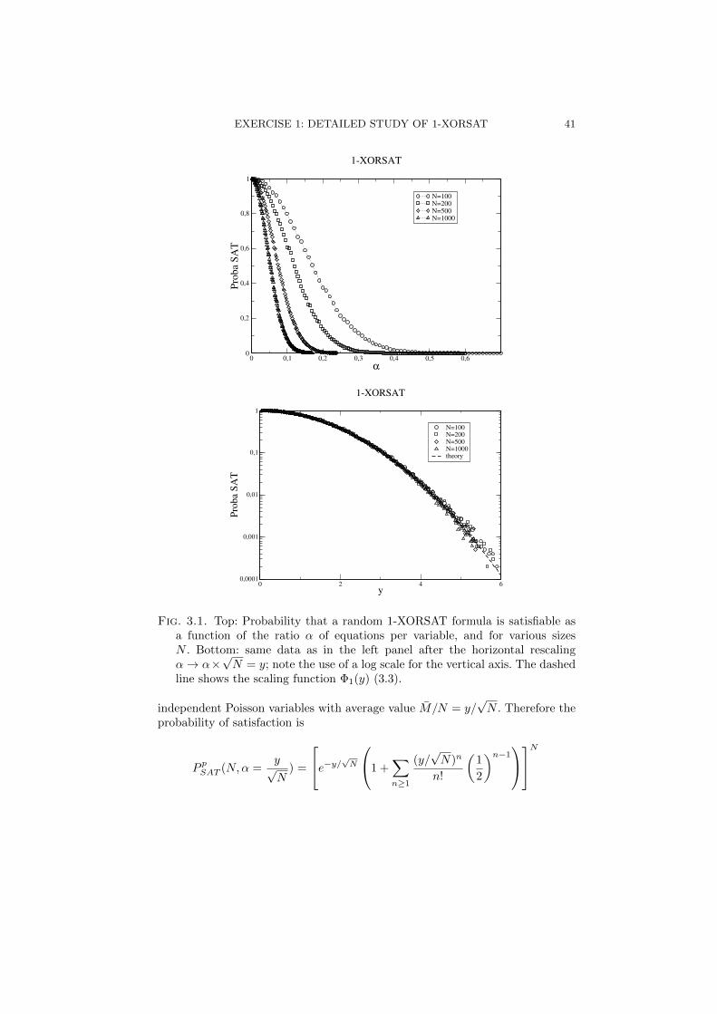
Figure 3.1(top) shows the probability PSAT that a randomly extracted 1-XORSATformula is satisfiable as a function of the ratio α, and for sizes N ranging from100 to 1000. We see that PSAT is a decreasing function of α and N .

Consider the subformula made of the ni equations with first member equalto xi. This formula is always satisfiable if ni = 0 or ni = 1. If ni ≥ 2 theformula is satisfiable if and only if all second members are equal (to 0, or to1), an event with probability ( 12 )

ni−1 decreasing exponentially with the numberof equations. Hence we have to consider the following variant of the celebratedBirthday problem16. Consider a year with a number N of days, how should scalethe number M of students in a class to be sure that no two students have thesame birthday date?

p =M−1

i=0

1− i

N

= exp

−M(M − 1)

2N+O(M3/N2)

. (3.1)

Hence we expect a cross-over from large to small p when M crosses the scalingregime

√N . Going back to the 1-XORSAT model we expect PSAT to have a non

zero limit value when the number of equations and variables are both sent toinfinity at a fixed ratio y = M/

√N . In other words, random 1-XORSAT formulas

with N variables, M equations or with, say, 100×N variables, 10×M equationsshould have roughly the same probabilities of being satisfiable. To check thishypothesis we replot the data in Figure 3.1 after multiplication of the abscissaof each point by

√N (to keep y fixed instead of α). The outcome is shown in the

bottom panel of Figure 3.1. Data obtained for various sizes nicely collapse on asingle limit curve function of y.

The calculation of this limit function, usually called scaling function, is donehereafter in the fixed-probability 1-XORSAT model where the number of equa-tions is a Poisson variable of mean value M = y

√N . We will discuss the equiv-

alence between the fixed-probability and the fixed-size ensembles later. In thefixed-probability ensemble the numbers ni of occurence of each variable xi are

16The Birthday problem is a classical elementary probability problem: given a class with M

students, what is the probability that at least two of them have the same birthday date? Theanswer for M = 25 is p 57%, while a much lower value is expected on intuitive grounds whenM is much smaller than the number N = 365 of days in a year.

EXERCISE 1: DETAILED STUDY OF 1-XORSAT 41

0 0,1 0,2 0,3 0,4 0,5 0,6

α

0

0,2

0,4

0,6

0,8

1

Pro

ba S

AT

N=100N=200N=500N=1000

1-XORSAT

0 2 4 6y

0,0001

0,001

0,01

0,1

1

Pro

ba

SA

T

N=100N=200N=500N=1000theory

1-XORSAT

Fig. 3.1. Top: Probability that a random 1-XORSAT formula is satisfiable asa function of the ratio α of equations per variable, and for various sizesN . Bottom: same data as in the left panel after the horizontal rescalingα → α×

√N = y; note the use of a log scale for the vertical axis. The dashed

line shows the scaling function Φ1(y) (3.3).

independent Poisson variables with average value M/N = y/√N . Therefore the

probability of satisfaction is

P p

SAT(N,α =

y√N

) =

e−y/√N

1 +

n≥1

(y/√N)n

n!

1

2

n−1

N

42 SOLUTIONS TO EXERCISES

=2e−y/(2

√N) − e−y/

√N

N, (3.2)

where the p subscript denotes the use of the fixed-probability ensemble. Weobtain the desired scaling function

Φ1(y) ≡ limN→∞

lnP p

SAT(N,α =

y√N

) = −y2

4, (3.3)

in excellent agreement with the rescaled data of Figure 3.1 (bottom) [?].For finite but large N there is a tiny probability that a randomly extracted

formula is actually satisifiable even when α > 0. A natural question is to char-acterize the ‘rate’ at which PSAT tends to zero as N increases (at fixed α).Answering to such questions is the very scope of large deviation theory. Lookingfor events with very small probabilities is not only interesting from an academicpoint of view, but can also be crucial in practical applications.

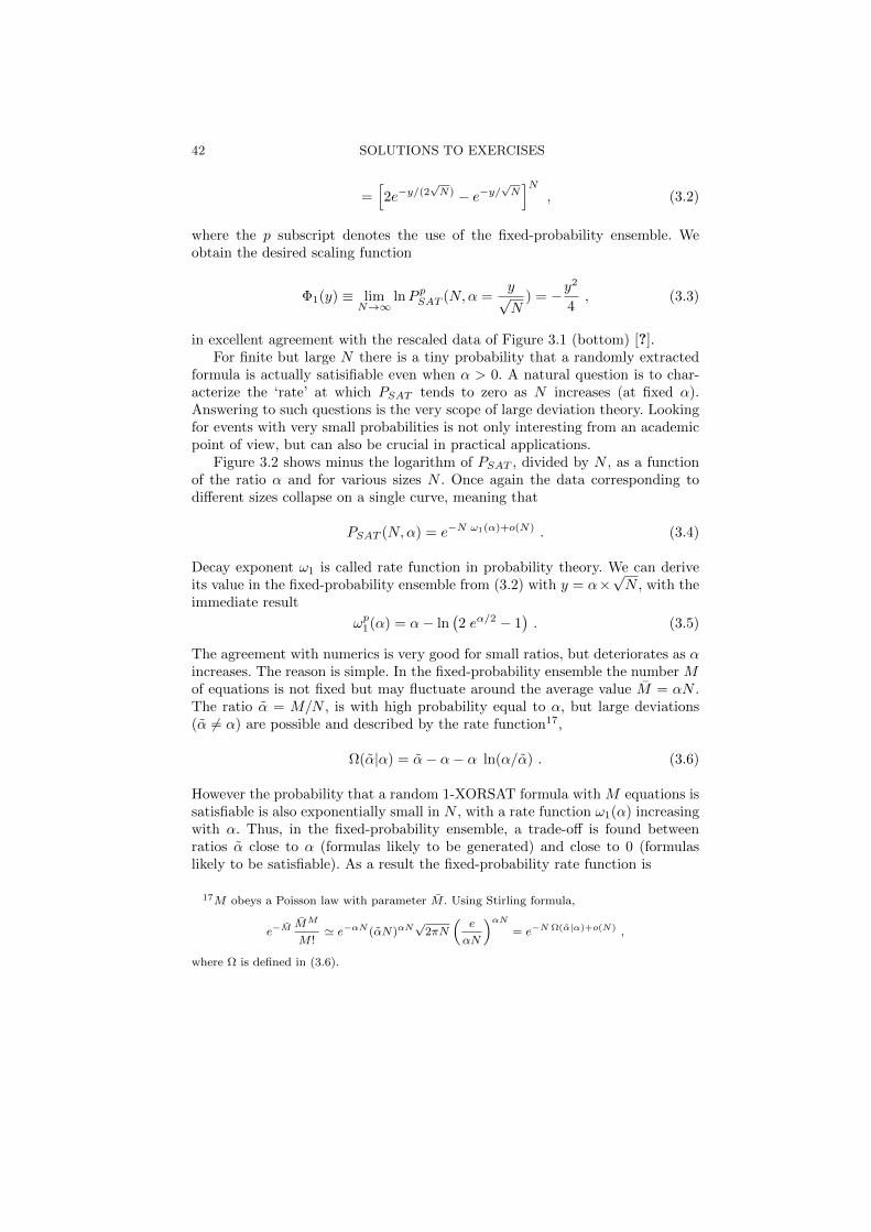
Figure 3.2 shows minus the logarithm of PSAT , divided by N , as a functionof the ratio α and for various sizes N . Once again the data corresponding todifferent sizes collapse on a single curve, meaning that

PSAT (N,α) = e−N ω1(α)+o(N) . (3.4)

Decay exponent ω1 is called rate function in probability theory. We can deriveits value in the fixed-probability ensemble from (3.2) with y = α×

√N , with the

immediate result

ωp

1(α) = α− ln2 eα/2 − 1

. (3.5)

The agreement with numerics is very good for small ratios, but deteriorates as αincreases. The reason is simple. In the fixed-probability ensemble the number Mof equations is not fixed but may fluctuate around the average value M = αN .The ratio α = M/N , is with high probability equal to α, but large deviations(α = α) are possible and described by the rate function17,

Ω(α|α) = α− α− α ln(α/α) . (3.6)

However the probability that a random 1-XORSAT formula with M equations issatisfiable is also exponentially small in N , with a rate function ω1(α) increasingwith α. Thus, in the fixed-probability ensemble, a trade-off is found betweenratios α close to α (formulas likely to be generated) and close to 0 (formulaslikely to be satisfiable). As a result the fixed-probability rate function is

17M obeys a Poisson law with parameter M . Using Stirling formula,

e−M MM

M ! e

−αN (αN)αN√2πN

e

αN

αN

= e−N Ω(α|α)+o(N)

,

where Ω is defined in (3.6).

EXERCISE 2: DYNAMICS OF THE UC HEURISTICS 43

0 0,2 0,4 0,6

α

0

0,05

0,1-l

n(P

rob

a S

AT

)/N

N=100N=200N=500N=1000fixed M ensemblePoissonian ensemble

1-XORSAT

Fig. 3.2. Same data as Figure 3.1 with: logarithmic scale on the vertical axis,and rescaling by −1/N . The scaling functions ω1 (3.7) and ωp

1 (3.5) for,respectively, the fixed-size and fixed-probability ensembles are shown.

ωp

1(α) = minα

ω1(α) + Ω(α|α)

, (3.7)

and is smaller than ω1(α). It is an easy check that the optimal ratio α∗ =α/(2 − e−α/2) < α as expected. Inverting (3.7) we deduce the rate function ω1

in the fixed-size ensemble, in excellent agreement with numerics (Figure 3.2).This example underlines that thermodynamically equivalent ensembles have tobe considered with care as far as rare events are concerned.

Remark that, when α → 0, α = α + O(α2), and ωp

1(α) = ω1(α) + O(α3).This common value coincides with the scaling function −Φ1(α) (3.3). This iden-tity is expected on general basis, and justifies the agreement between the fixed-probability scaling function and the numerics based on the fixed-size ensemble(Figure 3.1, right).

3.2 Exercise 2: dynamics of the UC heuristics

Let α0 denote the equation per variable ratio of the 3-XORSAT instance to besolved. We call Ej(T ) the number of j–equations (including j variables) after Tvariables have been assigned by the solving procedure. T will be called hereafter‘time’, not to be confused with the computational effort. At time T = 0 we haveE3(0) = α0N , E2(0) = E1(0) = 0. Assume that the variable x assigned at timeT is chosen from a single-variable clause, that is, independently of the j-equationcontent. Call nj(T ) the number of occurrences of x in j-equations (j = 2, 3). Theevolution equations for the populations of 2-,3-equations read


E3(T + 1) = E3(T )− n3(T ) , E2(T + 1) = E2(T )− n2(T ) + n3(T ) . (3.8)

Flows n2, n3 are of course random variables that depend on the instance underconsideration at time T , and on the choice of variable done by UC. What aretheir distributions? At time T there remain N−T untouched variables; x appearsin any of the Ej(T ) j-equation with probability pj =

j

N−T, independently of the

other equations. In the large N limit and at fixed fraction of assigned variables,t = T

N, the binomial distribution converges to a Poisson law with mean

njT =j ej1− t

where ej =Ej(T )

N(3.9)

is the density of j-equations at time T . The key remark is that, when N → ∞, ejis a slowly varying and non stochastic quantity and is a function of the fractiont = T

Nrather than T itself. Let us iterate (3.8) between times T0 = tN and

T0 + ∆T where 1 ∆T N e.g. ∆T = O(√N). Then the change ∆E3 in

the number of 3-equations is (minus) the sum of the stochastic variables nj(T )for T = T0, T0 + 1, . . . , T0 + ∆T . As these variables are uncorrelated Poissonvariables with O(1) mean (3.9) ∆E3 will be of the order of ∆T , and the changein the density e3 will be of order of ∆T/N → 0. Applying central limit theorem∆E3/∆T will be almost surely equal to −n3t given by (3.9) and with theequation density measured at reduced time t. The argument can be extendedto 2-equations, and we conclude that e2, e3 are deterministic (self-averaging)quantities obeying the two coupled differential equations

de3dt

(t) = − 3 e31− t

,de3dt

(t) =3 e31− t

− 2 e21− t

. (3.10)

Those equations, together with the initial condition e3(0) = α0, e2(0) = 0 canbe easily solved,

e3(t) = α0(1− t)3 , e2(t) = 3α0 t (1− t)2 . (3.11)

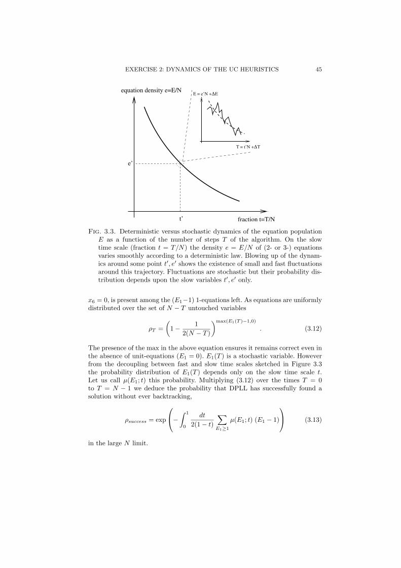
To sum up, the dynamical evolution of the equation populations may be seen as aslow and deterministic evolution of the equation densities to which are superim-posed fast, small fluctuations. The distribution of the fluctuations adiabaticallyfollows the slow trajectory. This scenario is pictured in Figure 3.3.

The trajectories we have derived in the previous Section are correct providedno contradiction emerges. But contradictions may happen as soon as there areE1 = 2 unit-equations, and are all the more likely than E1 is large. Actuallythe set of 1-equations form a 1-XORSAT instance which is unsatisfiable with afinite probability as soon as E1 is of the order of

√N from the results of Exercise

1. Assume now that E1(T ) N after T variables have been assigned, whatis the probability ρT that no contradiction emerges when the T th variable isassigned by UC? This probability is clearly one when E1 = 0. When E1 ≥ 1 wepick up a 1-equation, say, x6 = 1, and wonder whether the opposite 1-equation,


t’

e’

fraction t=T/N

∆

∆T = t’N + T

E = e’N + Eequation density e=E/N

Fig. 3.3. Deterministic versus stochastic dynamics of the equation populationE as a function of the number of steps T of the algorithm. On the slowtime scale (fraction t = T/N) the density e = E/N of (2- or 3-) equationsvaries smoothly according to a deterministic law. Blowing up of the dynam-ics around some point t, e shows the existence of small and fast fluctuationsaround this trajectory. Fluctuations are stochastic but their probability dis-tribution depends upon the slow variables t, e only.

x6 = 0, is present among the (E1−1) 1-equations left. As equations are uniformlydistributed over the set of N − T untouched variables

ρT =

1− 1

2(N − T )

max(E1(T )−1,0)

. (3.12)

The presence of the max in the above equation ensures it remains correct even inthe absence of unit-equations (E1 = 0). E1(T ) is a stochastic variable. Howeverfrom the decoupling between fast and slow time scales sketched in Figure 3.3the probability distribution of E1(T ) depends only on the slow time scale t.Let us call µ(E1; t) this probability. Multiplying (3.12) over the times T = 0to T = N − 1 we deduce the probability that DPLL has successfully found asolution without ever backtracking,

ρsuccess = exp

− 1

0

dt

2(1− t)

E1≥1

µ(E1; t) (E1 − 1)

(3.13)

in the large N limit.


1E’ 1E’0

n 2

E1

1s1

2n

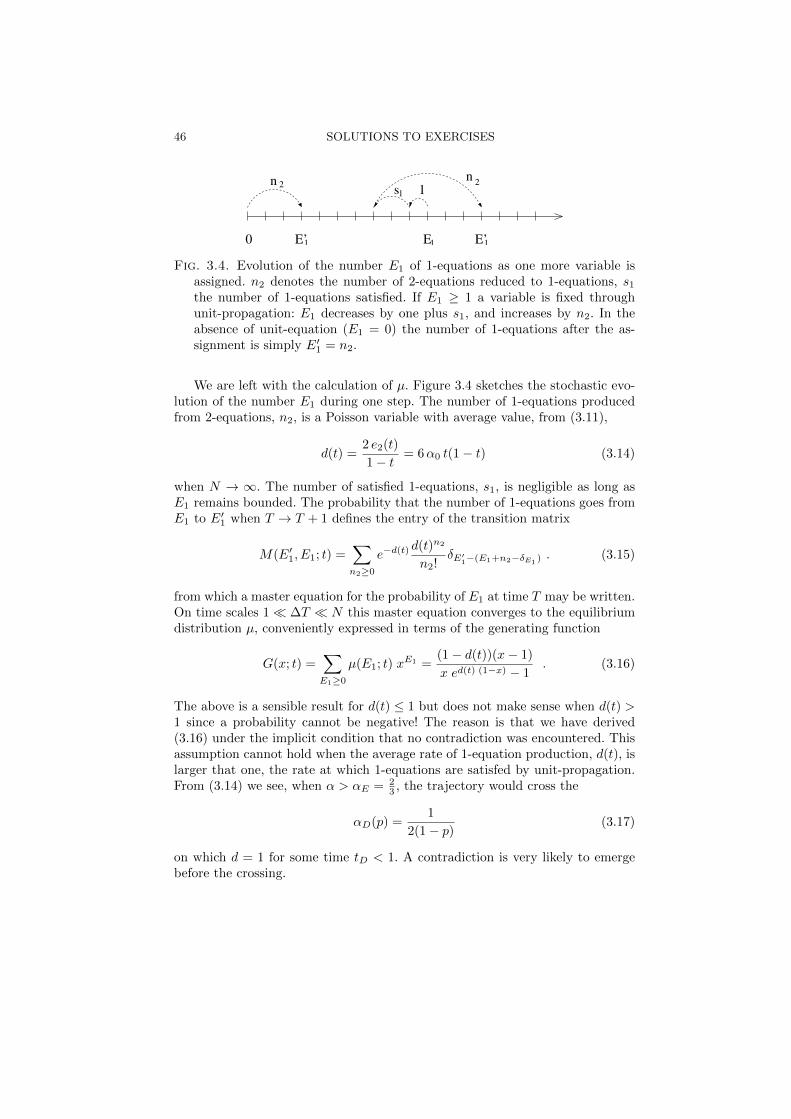
Fig. 3.4. Evolution of the number E1 of 1-equations as one more variable isassigned. n2 denotes the number of 2-equations reduced to 1-equations, s1the number of 1-equations satisfied. If E1 ≥ 1 a variable is fixed throughunit-propagation: E1 decreases by one plus s1, and increases by n2. In theabsence of unit-equation (E1 = 0) the number of 1-equations after the as-signment is simply E

1 = n2.

We are left with the calculation of µ. Figure 3.4 sketches the stochastic evo-lution of the number E1 during one step. The number of 1-equations producedfrom 2-equations, n2, is a Poisson variable with average value, from (3.11),

d(t) =2 e2(t)

1− t= 6α0 t(1− t) (3.14)

when N → ∞. The number of satisfied 1-equations, s1, is negligible as long asE1 remains bounded. The probability that the number of 1-equations goes fromE1 to E

1 when T → T + 1 defines the entry of the transition matrix

M(E1, E1; t) =

n2≥0

e−d(t) d(t)n2

n2!δE

1−(E1+n2−δE1 ). (3.15)

from which a master equation for the probability of E1 at time T may be written.On time scales 1 ∆T N this master equation converges to the equilibriumdistribution µ, conveniently expressed in terms of the generating function

G(x; t) =

E1≥0

µ(E1; t) xE1 =

(1− d(t))(x− 1)

x ed(t) (1−x) − 1. (3.16)

The above is a sensible result for d(t) ≤ 1 but does not make sense when d(t) >1 since a probability cannot be negative! The reason is that we have derived(3.16) under the implicit condition that no contradiction was encountered. Thisassumption cannot hold when the average rate of 1-equation production, d(t), islarger that one, the rate at which 1-equations are satisfed by unit-propagation.From (3.14) we see, when α > αE = 2

3 , the trajectory would cross the

αD(p) =1

2(1− p)(3.17)

on which d = 1 for some time tD < 1. A contradiction is very likely to emergebefore the crossing.


When α < αE d remains smaller than unity at any time. In this regime theprobability of success reads, using (3.13) and (3.16),

ρsuccess = exp

3α

4− 1

2

3α

2− 3αtanh−1

3α

2− 3α

. (3.18)

ρsuccess is a decreasing function of the ratio α, down from unity for α = 0 tozero for α = αE . In can be shown that, right at αE , ρsuccess ∼ exp(−Cst×N

16 )

decreases as a stretched exponential of the size. The value of the exponent,and its robustness against the splitting heuristics are explained in Deroulers,Monasson, Critical behaviour of combinatorial search algorithm and the unit-clause universality class, Europhysics Letters 68, 153 (2004).

Documents

RANDOM GRAPHS: DYNAMICAL PROCESSES AND REPLICA …