Random points on the sphere - UBjmarzo/Bcn15.pdf · For large number of \well distributed" points, they appear to arrange ... Random points on the sphere

$Page 1: Random points on the sphere - UBjmarzo/Bcn15.pdf · For large number of \well distributed" points, they appear to arrange ... Random points on the sphere$
Random points on the sphere

C. Beltran (U. Cantabria)J. Marzo (U. Barcelona)

& J. Ortega-Cerda (U. Barcelona)

“Well distributed” points on the sphere

Sd = {x = (x1, . . . , xd+1) ∈ Rd+1 : x21 + · · ·+ x2

d+1 = 1}

529 random uniform points


Sd = {x = (x1, . . . , xd+1) ∈ Rd+1 : x21 + · · ·+ x2

d+1 = 1}

Rob Womersley web http://web.maths.unsw.edu.au/ rsw/Sphere/ 529 Fekete points


Sd = {x = (x1, . . . , xd+1) ∈ Rd+1 : x21 + · · ·+ x2

d+1 = 1}

529 points points harmonic ensemble

Topological restriction

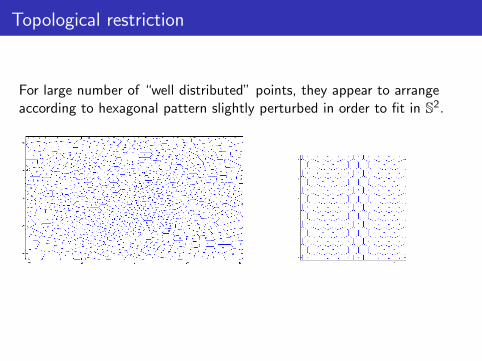
For large number of “well distributed” points, they appear to arrangeaccording to hexagonal pattern slightly perturbed in order to fit in S2.

Euler characteristic formula F − E + V = 2.

Topological restriction

For large number of “well distributed” points, they appear to arrangeaccording to hexagonal pattern slightly perturbed in order to fit in S2.

Euler characteristic formula F − E + V = 2.

Riesz energies

For a given collection of points x1, . . . , xn ∈ Sd and s > 0 thediscrete s-energy associated to the set x = {x1, . . . , xn} is

Es(x) =∑i 6=j

1

‖xi − xj‖s.

Minimal s-energy

E(s, n) = infx∈(Sd )n

Es(x).

Discrete logarithmic energy and minimal discrete logarithmicenergy

E0(x) =∑i 6=j

log1

‖xi − xj‖, E(0, n) = inf

xE0(x).

0 < s < d Thomson problem: d = 2, s = 1 Coulomb (andgeneralizations).s → +∞ Tammes problem. Best packing.Logarithmic case s = 0, d = 2, (elliptic) Fekete points.

Sandier and Serfaty work about renormalized energies and itsminimizers.Smale 7th problem.

A. Abrikosov extended Ginzburg-Landau model for superconductivityto fit with some experimental measurements. In this extension hepredicted the appearance of local defects of superconductivity calledvortices. These vortices repel each other and arrange into a triangularlattice.

H. F. Hess et al. Bell Labs Phys. Rev. Lett. 62, 214 (1989)

0 < s < d Thomson problem: d = 2, s = 1 Coulomb (andgeneralizations).s → +∞ Tammes problem. Best packing.Logarithmic case s = 0, d = 2, (elliptic) Fekete points.

Sandier and Serfaty work about renormalized energies and itsminimizers.Smale 7th problem.

A. Abrikosov extended Ginzburg-Landau model for superconductivityto fit with some experimental measurements. In this extension hepredicted the appearance of local defects of superconductivity calledvortices. These vortices repel each other and arrange into a triangularlattice.

H. F. Hess et al. Bell Labs Phys. Rev. Lett. 62, 214 (1989)

Mathematical model: Sandier and Serfaty (2014) work aboutrenormalized energies. Abrikosov (triangular) lattices are minimizersfor the renormalized energy among lattices. They conjectured thatthey are also global minimizers.

Until 2014 it was known (Wagner, Kuijlaars, Saff) that for somea < A < 0

an ≤ E(0, n)−(

1

2− log 2

)n2 +

n

2log n ≤ An, n→∞.

Brauchart, Hardin and Saff conjectured that

E(0, n) =

(1

2− log 2

)n2 − n

2log n + Cn + o(n), n→∞,

and

C = 2 log 2 +1

2log

2

3+ 3 log

√π

Γ(1/3)= −0.055605...

Betermin and Sandier show that C exists and both conjectures areequivalent.

Mathematical model: Sandier and Serfaty (2014) work aboutrenormalized energies. Abrikosov (triangular) lattices are minimizersfor the renormalized energy among lattices. They conjectured thatthey are also global minimizers.Until 2014 it was known (Wagner, Kuijlaars, Saff) that for somea < A < 0

an ≤ E(0, n)−(

1

2− log 2

)n2 +

n



E(0, n) =

(1

2− log 2

)n2 − n

2log n + Cn + o(n), n→∞,

and

C = 2 log 2 +1

2log

2

3+ 3 log

√π

Γ(1/3)= −0.055605...


Mathematical model: Sandier and Serfaty (2014) work aboutrenormalized energies. Abrikosov (triangular) lattices are minimizersfor the renormalized energy among lattices. They conjectured thatthey are also global minimizers.Until 2014 it was known (Wagner, Kuijlaars, Saff) that for somea < A < 0

an ≤ E(0, n)−(

1

2− log 2

)n2 +

n



E(0, n) =

(1

2− log 2

)n2 − n

2log n + Cn + o(n), n→∞,

and

C = 2 log 2 +1

2log

2

3+ 3 log

√π

Γ(1/3)= −0.055605...


s = 0 elliptic Fekete points (Smale 7th problem)

E0(x)− E(0, n) ≤ c log n.

Asymptotic behavior of the Riesz energies when n→∞

We want computable examples. Random configurations...but sets ofindependent uniformly random points exhibit clumping.

s = 0 elliptic Fekete points (Smale 7th problem)

E0(x)− E(0, n) ≤ c log n.

Asymptotic behavior of the Riesz energies when n→∞

We want computable examples. Random configurations...but sets ofindependent uniformly random points exhibit clumping.

Determinantal point process (Macchi 70’s)

Let µ be the normalized Lebesgue surface measure in a space X , inour case X = Sd , µ(X ) = 1.

Given a function (kernel) K : X × X −→ C such that:

K (x , y) = K (y , x)

Reproducing property∫X

K (x , y)K (y , z)dµ(y) = K (x , z)

Trace ∫X

K (x , x)dµ(x) = n

Then

f (x1, . . . , xn) =1

n!det(K (xi , xj))1≤i ,j≤n

is a density function in X .

Determinantal point process

Take φ1, . . . , φn ON system in L2(X ) then

K (x , y) =n∑

i=1

φi (x)φi (y),

satisfies the properties.

Example:Circular unitary ensemble (CUE). For X = S1, take φk(θ) = e ikθ then

K (x , y) =sin((n+ 1

2)(θ−φ))

sin( 12

(θ−φ))defines the density

f (θ1, . . . , θn) =1

n!

∏j<k

|e iθk − e iθj |2.

Weyl and Dyson: the eigenvalues of n × n unitary matrices drawnaccording to the Haar measure have a CUE distribution.

Determinantal point process

Take φ1, . . . , φn ON system in L2(X ) then

K (x , y) =n∑

i=1

φi (x)φi (y),

satisfies the properties.

Example:Circular unitary ensemble (CUE). For X = S1, take φk(θ) = e ikθ then

K (x , y) =sin((n+ 1

2)(θ−φ))

sin( 12

(θ−φ))defines the density

f (θ1, . . . , θn) =1

n!

∏j<k

|e iθk − e iθj |2.

Weyl and Dyson: the eigenvalues of n × n unitary matrices drawnaccording to the Haar measure have a CUE distribution.

Random matrix theory, Quantum physics, Machine learning...

By the HKPV (Ben Hough-Krishnapur-Peres-Virag) algorithm theseprocesses are “easy” to sample.

Spherical ensemble in S2: generalized eigenvalues of random n × nmatrices A,B with independent complex Gaussian entries (i.e.eigenvalues of A−1B).It is a determinantal process (Krishnapur) in the plane and by thestereographic projection defines a point process in S2 with density

f (p1, . . . , pn) =∏j<k

|pj − pk |2, pi ∈ R3.

Alishashi-Zamani (15).

Random matrix theory, Quantum physics, Machine learning...

By the HKPV (Ben Hough-Krishnapur-Peres-Virag) algorithm theseprocesses are “easy” to sample.

Spherical ensemble in S2: generalized eigenvalues of random n × nmatrices A,B with independent complex Gaussian entries (i.e.eigenvalues of A−1B).It is a determinantal process (Krishnapur) in the plane and by thestereographic projection defines a point process in S2 with density

f (p1, . . . , pn) =∏j<k

|pj − pk |2, pi ∈ R3.

Alishashi-Zamani (15).

25281 = 1592 points from the spherical ensemble

The harmonic ensemble in Sd

Let ΠL be the space of spherical harmonics of degree at most L in Sd(i.e. polynomials in Rd+1 of degree at most L restricted to Sd).

By Christoffel-Darboux formula the reproducing kernel of ΠL

KL(x , y) =πL(L+ d

2L

)P(1+λ,λ)L (〈x , y〉), x , y ∈ Sd ,

where λ = d−22 and the Jacobi polynomials are P

(1+λ,λ)L (1) =

(L+ d2

L

).

By definition

P(x) = 〈P,KL(·, x)〉 =

∫Sd

KL(x , y)P(y)dµ(y), for P ∈ ΠL.

Then

dim ΠL = πL =2

Γ(d + 1)Ld + o(Ld),

and KL(x , x) = πL for every x ∈ Sd .


Let ΠL be the space of spherical harmonics of degree at most L in Sd(i.e. polynomials in Rd+1 of degree at most L restricted to Sd).

By Christoffel-Darboux formula the reproducing kernel of ΠL

KL(x , y) =πL(L+ d

2L

)P(1+λ,λ)L (〈x , y〉), x , y ∈ Sd ,

where λ = d−22 and the Jacobi polynomials are P

(1+λ,λ)L (1) =

(L+ d2

L

).

By definition

P(x) = 〈P,KL(·, x)〉 =

∫Sd

KL(x , y)P(y)dµ(y), for P ∈ ΠL.

Then

dim ΠL = πL =2

Γ(d + 1)Ld + o(Ld),

and KL(x , x) = πL for every x ∈ Sd .


The harmonic ensemble is the determinantal point process in Sd withπL points a.s. induced by the kernel

KL(x , y) =πL(L+ d

2L

)P(1+λ,λ)L (〈x , y〉)

.

We study diferent aspects of this process:

Expected Riesz energies

Linear statistics and spherical cap discrepancy

Separation distance

Energy optimality among isotropic processes



KL(x , y) =πL(L+ d

2L

)P(1+λ,λ)L (〈x , y〉)

.




Separation distance




KL(x , y) =πL(L+ d

2L

)P(1+λ,λ)L (〈x , y〉)

.




Separation distance


Let K be a kernel with trace n, and let x1, . . . , xn be generated by theassociated determinantal point process.

E(s, n) ≤ Ex∈(Sd )n

∑i 6=j

1

‖xi − xj‖s

For any measurable f : Sd × Sd → [0,∞) we have

E

∑i 6=j

f (xi , xj)

=

∫(Sd )2

(K (x , x)K (y , y)− |K (x , y)|2

)f (x , y)dµ(x)dµ(y).

Take f (x , y) = ‖x − y‖−s for 0 < s < d (and limiting cases s = 0, d).

Continuous s-energy for the normalized Lebesgue measure is(0 < s < d)

Vs(Sd) =

∫Sd

∫Sd

1

‖x − y‖s dµ(x) dµ(y) = 2d−s−1 Γ(d+1

2

)Γ(d−s

2

)√πΓ(d − s

2

) .



∑i 6=j

1

‖xi − xj‖s


E

∑i 6=j

f (xi , xj)

=

∫(Sd )2

(K (x , x)K (y , y)− |K (x , y)|2




Vs(Sd) =

∫Sd

∫Sd

1

‖x − y‖s dµ(x) dµ(y) = 2d−s−1 Γ(d+1

2

)Γ(d−s

2

)√πΓ(d − s

2

) .



∑i 6=j

1

‖xi − xj‖s


E

∑i 6=j

f (xi , xj)

=

∫(Sd )2

(K (x , x)K (y , y)− |K (x , y)|2




Vs(Sd) =

∫Sd

∫Sd

1

‖x − y‖s dµ(x) dµ(y) = 2d−s−1 Γ(d+1

2

)Γ(d−s

2

)√πΓ(d − s

2

) .



∑i 6=j

1

‖xi − xj‖s


E

∑i 6=j

f (xi , xj)

=

∫(Sd )2

(K (x , x)K (y , y)− |K (x , y)|2




Vs(Sd) =

∫Sd

∫Sd

1

‖x − y‖s dµ(x) dµ(y) = 2d−s−1 Γ(d+1

2

)Γ(d−s

2

)√πΓ(d − s

2

) .

It is known that (Alexander, Stolarsky, Wagner, Kuijlaars, Saff,Brauchart) for d ≥ 2 and 0 < s < d there exist constants C , c > 0such that

−cn1+s/d ≤ E(s, n)− Vs(Sd)n2 ≤ −Cn1+s/d ,

for n ≥ 2.

Conjecture (BHS) : there is a constant As,d such that

E(s, n) = Vs(Sd)n2 +As,d

ωs/dd

n1+s/d + o(n1+s/d).

Furthermore, when d = 2, 4, 8, 24

As,d = |Λd |s/dζΛd(s),

where |Λd | stands for the co-volume and ζΛd(s) for the Epstein zeta

function of the lattice Λd . Here Λd denotes the triangular lattice ford = 2, the root lattices D4 for d = 4 and E8 for d = 8 and the Leechlattice for d = 24.Recall that in the logarithmic case the constant exist.



for n ≥ 2.Conjecture (BHS) : there is a constant As,d such that


ωs/dd

n1+s/d + o(n1+s/d).




function of the lattice Λd . Here Λd denotes the triangular lattice ford = 2, the root lattices D4 for d = 4 and E8 for d = 8 and the Leechlattice for d = 24.

Recall that in the logarithmic case the constant exist.



for n ≥ 2.Conjecture (BHS) : there is a constant As,d such that


ωs/dd

n1+s/d + o(n1+s/d).




function of the lattice Λd . Here Λd denotes the triangular lattice ford = 2, the root lattices D4 for d = 4 and E8 for d = 8 and the Leechlattice for d = 24.Recall that in the logarithmic case the constant exist.

Computing the expected energy

KL(x , y) reproducing kernel of the space of polynomials of degree atmost L in Sd

E

∑i 6=j

1

‖xi − xj‖s

=

∫(Sd )2

KL(x , x)KL(y , y)− |KL(x , y)|2‖x − y‖s dµ(x)dµ(y),

with

KL(x , y) = CLP(1+λ,λ)L (〈x , y〉),

then∫Sd

|KL(x ,N)|2‖x − N‖s dµ(x) = CL,s,d

∫ 1

−1P

(1+λ,λ)L (t)2(1− t)λ−

s2 (1 + t)λ dt.



E

∑i 6=j

1

‖xi − xj‖s

=

∫(Sd )2


with

KL(x , y) = CLP(1+λ,λ)L (〈x , y〉),

then∫Sd


∫ 1

−1P

(1+λ,λ)L (t)2(1− t)λ−

s2 (1 + t)λ dt.



E

∑i 6=j

1

‖xi − xj‖s

=

∫(Sd )2


with

KL(x , y) = CLP(1+λ,λ)L (〈x , y〉),

then∫Sd


∫ 1

−1P

(1+λ,λ)L (t)2(1− t)λ−

s2 (1 + t)λ dt.

From Erdelyi-Magnus-Oberhettinger-Tricomi 54

For integer p, q ≥ 0 and complex values ai , bj the generalizedhypergeometric function is

pFq(a1, . . . , ap; b1, . . . , bq; z) =∞∑n=0

(a1)n . . . (ap)n(b1)n . . . (bq)n

zn

n!,

where (·)n is the rising factorial or Pochhammer symbol

(x)n =Γ(x + n)

Γ(x).

From Erdelyi-Magnus-Oberhettinger-Tricomi 54

For integer p, q ≥ 0 and complex values ai , bj the generalizedhypergeometric function is

pFq(a1, . . . , ap; b1, . . . , bq; z) =∞∑n=0

(a1)n . . . (ap)n(b1)n . . . (bq)n

zn

n!,

where (·)n is the rising factorial or Pochhammer symbol

(x)n =Γ(x + n)

Γ(x).

In our case for n = πL ∼ Ld we get

4F3

(−L, d + L,

d − s

2,− s

2;

d

2+ 1, d − s

2+ L,− s

2− L; 1

)

=L∑

k=0

(−L)k(d + L)k(d−s2 )k(− s2 )k

(d2 + 1)k(d − s2 + L)k(− s

2 − L)k

1

k!.

When s is even(− s

2

)k

= (−1)k( s

2− k + 1

)k

= (−1)kΓ(s2 + 1

)Γ(s2 − k + 1

) = 0,

if k > s/2.

In our case for n = πL ∼ Ld we get

4F3

(−L, d + L,

d − s

2,− s

2;

d

2+ 1, d − s

2+ L,− s

2− L; 1

)

=L∑

k=0

(−L)k(d + L)k(d−s2 )k(− s2 )k

(d2 + 1)k(d − s2 + L)k(− s

2 − L)k

1

k!.

When s is even(− s

2

)k

= (−1)k( s

2− k + 1

)k

= (−1)kΓ(s2 + 1

)Γ(s2 − k + 1

) = 0,

if k > s/2.

We have

4F3

(−L, d + L,

d − s

2,− s

2;

d

2+ 1, d − s

2+ L,− s

2− L; 1

)

=

s/2∑k=0

(−L)k(d + L)k(d−s2 )k(− s2 )k

(d2 + 1)k(d − s2 + L)k(− s

2 − L)k

1

k!.

and we get for L→∞ ( for α ∈ R Γ(n + α) ∼ Γ(n)nα)

s/2∑k=0

(−L)k(d + L)k(d−s2 )k(− s2 )k

(d2 + 1)k(d − s2 + L)k(− s

2 − L)k

1

k!−→

+∞∑k=0

(d−s2 )k(− s2 )k

(d2 + 1)k

1

k!

= 2F1

(d − s

2,− s

2;

d

2+ 1; 1

)=

Γ(1 + d

2

)Γ (1 + s)

Γ(1 + s

2

)Γ(1 + d+s

2

) ,by Gauss theorem.

We have

4F3

(−L, d + L,

d − s

2,− s

2;

d

2+ 1, d − s

2+ L,− s

2− L; 1

)

=

s/2∑k=0

(−L)k(d + L)k(d−s2 )k(− s2 )k

(d2 + 1)k(d − s2 + L)k(− s

2 − L)k

1

k!.


s/2∑k=0

(−L)k(d + L)k(d−s2 )k(− s2 )k

(d2 + 1)k(d − s2 + L)k(− s

2 − L)k

1

k!−→

+∞∑k=0

(d−s2 )k(− s2 )k

(d2 + 1)k

1

k!

= 2F1

(d − s

2,− s

2;

d

2+ 1; 1

)=

Γ(1 + d

2

)Γ (1 + s)

Γ(1 + s

2

)Γ(1 + d+s

2


We have

4F3

(−L, d + L,

d − s

2,− s

2;

d

2+ 1, d − s

2+ L,− s

2− L; 1

)

=

s/2∑k=0

(−L)k(d + L)k(d−s2 )k(− s2 )k

(d2 + 1)k(d − s2 + L)k(− s

2 − L)k

1

k!.


s/2∑k=0

(−L)k(d + L)k(d−s2 )k(− s2 )k

(d2 + 1)k(d − s2 + L)k(− s

2 − L)k

1

k!−→

+∞∑k=0

(d−s2 )k(− s2 )k

(d2 + 1)k

1

k!

= 2F1

(d − s

2,− s

2;

d

2+ 1; 1

)=

Γ(1 + d

2

)Γ (1 + s)

Γ(1 + s

2

)Γ(1 + d+s

2


Theorem

Let x = (x1, . . . , xn) where n = πL be drawn from the harmonicensemble. Then, for 0 < s < d ,

Ex∈(Sd )n(Es(x)) = Vs(Sd)n2 − Cs,dn1+s/d + o(n1+s/d),

for some explicit constant Cs,d > 0.

The general case (and the limiting cases) are more difficult: weimprove the constants or match the order (s=d).

For d = 2 the BHS conjecture is

E(s, n) = Vs(S2)n2 +(√

3/2)s/2ζΛ2(s)

(4π)s/2n1+s/2 + o(n1+s/2),

where ζΛ2(s) is the zeta function of the triangular lattice (DirichletL-series).

Theorem

Let x = (x1, . . . , xn) where n = πL be drawn from the harmonicensemble. Then, for 0 < s < d ,

Ex∈(Sd )n(Es(x)) = Vs(Sd)n2 − Cs,dn1+s/d + o(n1+s/d),

for some explicit constant Cs,d > 0.

The general case (and the limiting cases) are more difficult: weimprove the constants or match the order (s=d).For d = 2 the BHS conjecture is

E(s, n) = Vs(S2)n2 +(√

3/2)s/2ζΛ2(s)

(4π)s/2n1+s/2 + o(n1+s/2),

where ζΛ2(s) is the zeta function of the triangular lattice (DirichletL-series).

d=2

0.0 0.5 1.0 1.5 2.0

0

1

2

3

4

5

6

7

Figure : Graphic of − (√

3/2)s/2ζΛ2(s)

(4π)s/2 in black, 2−sΓ(1− s2 ) (spherical) in red,

the constant Cs,2 (harmonic) in green and 1/(2√

2π)s in blue.

Optimality

Could we find the best determinantal process? i.e. the kernel suchthat the expected energy is minimal?

Theorem (Macchi-Soshnikov)

An hermitic kernel K (x , y) locally trace class in L2(X ) corresponds toa determinantal pont process if and only if the eigenvalues are in [0, 1].

Theorem (Shirai-Takahashi)

In a determinantal process, the number of points that fall in acompact set D ⊂ X has the same distribution as a sum of independentrandom variables Bernouilli(λDi ), where λDi are the eigenvalues of theintegral operator defined by the kernel K (x , y) restricted to D.

Optimality






Optimality






The kernel

Some assumptions:

Invariant by rotations i.e.

d(x , y) = d(z , t) =⇒ K (x , y) = K (z , t), x , y , z , t ∈ Sd ,

and then K (〈x , y〉) for some K : [−1, 1] 7→ R.

We need that for any x1, . . . , xk ∈ Sd the matrix

(K (〈xi , xj〉))1≤i ,j≤k ,

is nonegative definite (sphere version of Bochner theorem).

If we want n points a.s. in Sd then all the eigenvalues must be 1(projection kernel).

The kernel

Some assumptions:





(K (〈xi , xj〉))1≤i ,j≤k ,



The kernel

Some assumptions:





(K (〈xi , xj〉))1≤i ,j≤k ,



The kernel

Some assumptions:





(K (〈xi , xj〉))1≤i ,j≤k ,



Schoenberg theorem (42)

We must have

K (x , y) = K (〈x , y〉), K (t) =∞∑k=0

akCd/2−1/2k (t),

where Cd/2−1/2k is a Gegenbauer polynomial and the ak ∈

[0, 2k+d−1

d−1

]satisfy:

trace(K ) = K (1) =∞∑k=0

ak

(d + k − 2

k

)<∞.

To have a projection kernel with with n points we take

ak ∈{

0,2k + d − 1

d − 1

}with

∞∑k=0

ak

(d + k − 2

k

)= n. (∗)

Schoenberg theorem (42)

We must have

K (x , y) = K (〈x , y〉), K (t) =∞∑k=0

akCd/2−1/2k (t),

where Cd/2−1/2k is a Gegenbauer polynomial and the ak ∈

[0, 2k+d−1

d−1

]satisfy:

trace(K ) = K (1) =∞∑k=0

ak

(d + k − 2

k

)<∞.

To have a projection kernel with with n points we take

ak ∈{

0,2k + d − 1

d − 1

}with

∞∑k=0

ak

(d + k − 2

k

)= n. (∗)

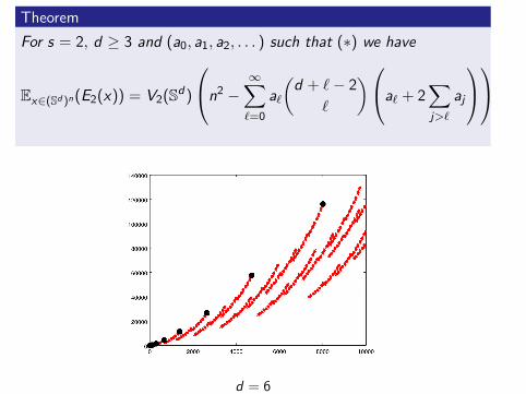
Theorem

For s = 2, d ≥ 3 and (a0, a1, a2, . . . ) such that (∗) we have

Ex∈(Sd )n(E2(x)) = V2(Sd)

n2 −∞∑`=0

a`

(d + `− 2

`

)a` + 2∑j>`

aj

Theorem



n2 −∞∑`=0

a`

(d + `− 2

`

)a` + 2∑j>`

aj

d = 4

Theorem



n2 −∞∑`=0

a`

(d + `− 2

`

)a` + 2∑j>`

aj

d = 6

Theorem

Let Ka and Kb be two kernels with coefficients a = (a0, a1, . . .) andb = (b0, b1, . . .) satifying conditions (∗). Let Ea and Eb denoterespectively the expected value of

E2(x) =∑i 6=j

1

‖xi − xj‖2,

when x = (x1, . . . , xn) is given by the determinantal point processassociated to Ka and Kb. Assume that for every i , j ∈ N we have:

if i < j , ai = 0 and aj > 0 then bi = 0. (1)

Then, Ea ≤ Eb, with strict inequality unless a = b. In particular, theharmonic kernel is optimal since (1) is trivially satisfied in that case.

Example. The harmonic kernel is optimal (d = 3)

We have

n = πL =L+1∑k=1

k2 =(2L + 3)(L + 2)(L + 1)

6∈ {5, 14, 30, 55, 91, 140 . . . }

We want to see that the maximum of∞∑k=1

xk∑k<j

kxk ,

for xk ∈ {0, k} with∞∑k=1

xkk = n,

is attained when xk = k for k = 1, . . . , L + 1.For example:

1+4+9+16=30=1+4+251+4+9+16+25+36=91=1+9+81


We have

n = πL =L+1∑k=1

k2 =(2L + 3)(L + 2)(L + 1)

6∈ {5, 14, 30, 55, 91, 140 . . . }


xk∑k<j

kxk ,


xkk = n,

is attained when xk = k for k = 1, . . . , L + 1.

For example:

1+4+9+16=30=1+4+251+4+9+16+25+36=91=1+9+81


We have

n = πL =L+1∑k=1

k2 =(2L + 3)(L + 2)(L + 1)

6∈ {5, 14, 30, 55, 91, 140 . . . }


xk∑k<j

kxk ,


xkk = n,

is attained when xk = k for k = 1, . . . , L + 1.For example:

1+4+9+16=30=1+4+251+4+9+16+25+36=91=1+9+81

We define two kinds of “movements” increasing∑∞

k=1 xk∑

k<j kxk .

Closing the gaps:

j j + 1 j + `− 1 j + `

j+s j+s+1 j + `j + s+ 2

Refilling:

j j + 1 j + `− 1 j + `

j j + 1 j + `− 1 j + `


k=1 xk∑

k<j kxk .Closing the gaps:

j j + 1 j + `− 1 j + `

j+s j+s+1 j + `j + s+ 2

Refilling:

j j + 1 j + `− 1 j + `

j j + 1 j + `− 1 j + `


k=1 xk∑

k<j kxk .Closing the gaps:

j j + 1 j + `− 1 j + `

j+s j+s+1 j + `j + s+ 2

Refilling:

j j + 1 j + `− 1 j + `

j j + 1 j + `− 1 j + `

Documents

Random points on the sphere - UBjmarzo/Bcn15.pdf · For large number of \well distributed" points, they appear to arrange ... Random points on the sphere