Embed Size (px)
Citation preview
Random ProcessLecture 7. Wide Sense Stationary Random
Processes
Husheng Li
Min Kao Department of Electrical Engineering and Computer ScienceUniversity of Tennessee, Knoxville
Spring, 2016
1/21
Hilbert Space Generated byStationary Process
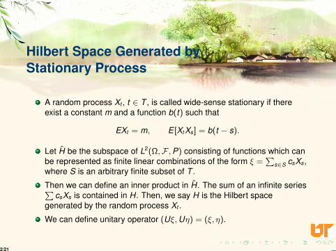
A random process Xt , t ∈ T , is called wide-sense stationary if thereexist a constant m and a function b(t) such that
EXt = m, E [XtXs] = b(t − s).
Let H be the subspace of L2(Ω,F ,P) consisting of functions which canbe represented as finite linear combinations of the form ξ =
∑s∈S csXs,
where S is an arbitrary finite subset of T .
Then we can define an inner product in H. The sum of an infinite series∑csXs is contained in H. Then, we say H is the Hilbert space
generated by the random process Xt .
We can define unitary operator (Uξ,Uη) = (ξ, η).
2/21
Law of Large Numbers
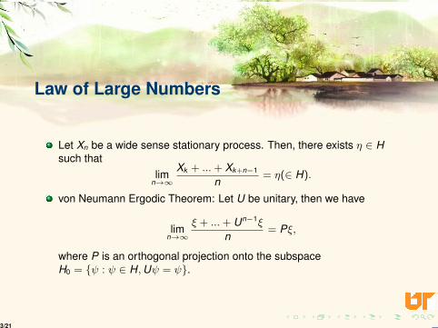
Let Xn be a wide sense stationary process. Then, there exists η ∈ Hsuch that
limn→∞
Xk + ...+ Xk+n−1
n= η(∈ H).
von Neumann Ergodic Theorem: Let U be unitary, then we have
limn→∞
ξ + ...+ Un−1ξ
n= Pξ,
where P is an orthogonal projection onto the subspaceH0 = ψ : ψ ∈ H,Uψ = ψ.
3/21
Bochner Theorem
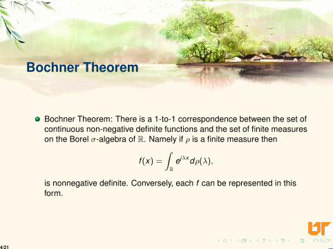
Bochner Theorem: There is a 1-to-1 correspondence between the set ofcontinuous non-negative definite functions and the set of finite measureson the Borel σ-algebra of R. Namely if ρ is a finite measure then
f (x) =
∫R
ejλx dρ(λ),
is nonnegative definite. Conversely, each f can be represented in thisform.
4/21
Spectrum Representation ofStationary RandomProcesses
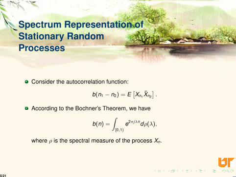
Consider the autocorrelation function:
b(n1 − n2) = E[Xn1 Xn2
].
According to the Bochner’s Theorem, we have
b(n) =
∫[0,1)
e2πjλndρ(λ),
where ρ is the spectral measure of the process Xn.
5/21
Spectrum Representation ofStationary RandomProcesses (Continued)
Theorem: Consider the space L2([0, 1),B([0, 1)), ρ) of square-integrablefunctions on [0, 1) (with respect to the measure ρ). There exists anisomorphism ψ : H → L2 if the spaces H and L2 such that
ψ(Uξ) = e2πjλψ(ξ).
Corollary: If ρ(0) = 0, then H0 = 0 and the time averages in the Lawof Large Numbers converge to zero.
6/21
Orthogonal RandomMeasures
Consider a Borel subset ∆ ⊂ [0, 1). Define
Z (∆) = ψ−1(X∆).
A function Z with values in L2(Ω,F ,P) defined on a σ-algebra is calledan orthogonal random measure if it satisfies two conditions. If Z is givenby the above definition, it is called the random spectral measure of theprocess Xn.
Then, we can define an integral with respect to an orthogonal randommeasure.
7/21
Linear Prediction
We consider stationary random processes with discrete time andassume that EXn = 0.
We define
Hk2k1
= closure
k2∑
n=k1
cnXn
.
Given m < k0, how to find the best approximation of Xk0 by using theelements in Hm
−∞.
8/21
Linear Predictors
We defineh−m = inf ‖X0 −
∑n≤−m
cnXn‖.
A random process Xn is called linearly non-deterministic if h−1 > 0.
A random process Xn is called linear regular if P−m−∞X0 → 0 if m→∞.
Theorem: A process Xn is linearly regular if and only if it is linearlynon-deterministic and ρ is absolutely continuous with respect to theLebesgue measure.
9/21
Kolmogorov-WienerTheorem
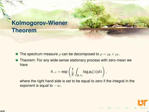
The spectrum measure ρ can be decomposed to ρ = ρ0 + ρ1.
Theorem: For any wide-sense stationary process with zero mean wehave
h−1 = exp
(12
∫[0,1)
log p0(λ)dλ
),
where the right hand side is set to be equal to zero if the integral in theexponent is equal to −∞.
10/21
Linear Filtering
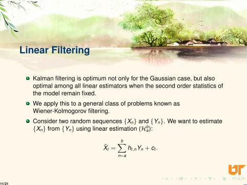
Kalman filtering is optimum not only for the Gaussian case, but alsooptimal among all linear estimators when the second order statistics ofthe model remain fixed.
We apply this to a general class of problems known asWiener-Kolmogorov filtering.
Consider two random sequences Xn and Yn. We want to estimateXn from Yn using linear estimation (Hb
a):
Xt =b∑
n=a
ht,nYn + ct .
11/21
MMSE and OrthogonalPrinciple
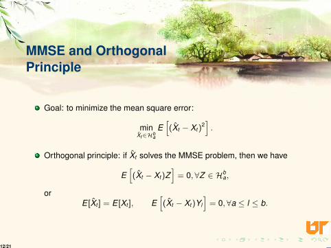
Goal: to minimize the mean square error:
minXt∈Hb
a
E[(Xt − Xt )
2].
Orthogonal principle: if Xt solves the MMSE problem, then we have
E[(Xt − Xt )Z
]= 0, ∀Z ∈ Hb
a,
orE [Xt ] = E [Xt ], E
[(Xt − Xt )Yl
]= 0, ∀a ≤ l ≤ b.
12/21
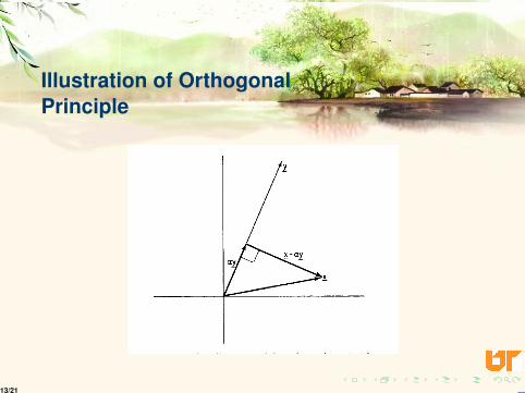
Illustration of OrthogonalPrinciple
13/21

How to Determine theCoefficients?
We can apply the orthogonal principle to determine the coefficients inthe linear estimation.
Wiener-Hopf Equation:
Cov(Xt ,Yl ) =b∑
n=a
ht,nCov(Yn,Yl ),
or the matrix form:σX ,Y (t) = ΣY ht .
14/21
Algorithms
Levinson Filtering: Levinson filtering is concerned with one-stepprediction of a random sequence whose second-order statistics arestationary in time:
CY (n, l) = CY (n − l , 0).
We want to estimate Yt from Yss<t , namely
Yt =t−1∑n=0
ht,nYn.
15/21
Wiener-Kolmogorov Filtering
Noncausal W-K filtering: We estimate Xt using observations Ys from−∞ to∞:
Xt =∞∑
n=−∞
ht,nYn.
The Wiener-Hopf equation becomes
CXY (τ) =∞∑
a=−∞
haCY (τ − a).
Can you see the convolution structure in the equation?
16/21
Frequency Domain
Carry out Fourier transformation for CXY , CY and ha and thus obtainφXY , φY and H.
The Wiener-Hopf equation becomes
φXY (w) = φY (w)H(w), −π ≤ w ≤ π.
Then, h(n) is obtained from the inverse transform of φXY (w)φY (w)
.
17/21
Causal Wiener-KolmogorovFiltering
The main drawback of the noncausal Wiener-Kolmogorov filtering is thatit requires all future observations. To make it causal, we have
Xt =t∑
n=−∞
ht,nYn,
which is denoted by Ht−∞. We can reuse ht,n of the noncausal filter,
namely truncation.
According to the orthogonality principle, we need
E [(Xt − Xt )Z ] = 0,
for all Z ∈ Ht−∞. This is true when Yt is uncorrelated.
18/21
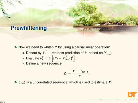
Prewhittening
Now we need to whiten Y by using a causal linear operation:
Denote by ˆYt|t−1 the best prediction of Yt based on Y t−1−∞.
Evaluate σ2t = E
[(Yt − ˆYt|t−1)2
].
Define a new sequence
Zn =Yt − ˆYt|t−1
σn.
Zn is a uncorrelated sequence, which is used to estimate Xt .
19/21
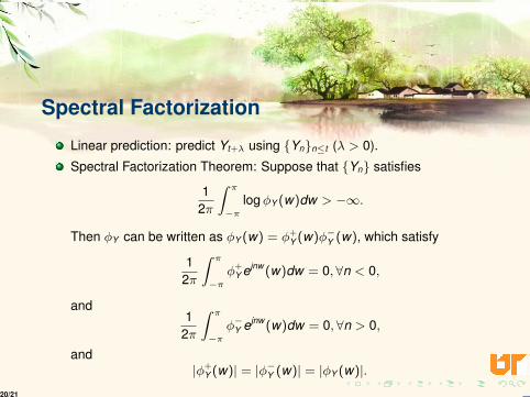
Spectral Factorization
Linear prediction: predict Yt+λ using Ynn≤t (λ > 0).
Spectral Factorization Theorem: Suppose that Yn satisfies
12π
∫ π
−πlogφY (w)dw > −∞.
Then φY can be written as φY (w) = φ+Y (w)φ−Y (w), which satisfy
12π
∫ π
−πφ+
Y ejnw (w)dw = 0, ∀n < 0,
and1
2π
∫ π
−πφ−Y ejnw (w)dw = 0,∀n > 0,
and|φ+
Y (w)| = |φ−Y (w)| = |φY (w)|.20/21
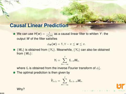
Causal Linear PredictionWe can use H(w) = 1
φ+Y (w)
as a causal linear filter to whiten Y : the
output W of the filter satisfies
φW (w) = 1, ∀ − π ≤ w ≤ π.
Wn is obtained from Yn. Meanwhile, Yn can also be obtainedfrom Wn:
Yt =t∑
n=−∞
ft−nWn,
where fn is obtained from the inverse Fourier transform of φ+Y .
The optimal prediction is then given by
Yt+λ =t∑
n=−∞
ft+λ−nWn.
Why?21/21