Random Processes — Why we Care

Gaussian Basics Random Processes Filtering of Random Processes Signal Space Concepts

Random Processes — Why we CareI Random processes describe signals that change randomly

over time.I Compare: deterministic signals can be described by a

mathematical expression that describes the signal exactlyfor all time.

I Example: x(t) = 3 cos(2pfct + p/4) with fc = 1GHz.I We will encounter three types of random processes in

communication systems:1. (nearly) deterministic signal with a random parameter —

Example: sinusoid with random phase.2. signals constructed from a sequence of random variables

— Example: digitally modulated signals with randomsymbols

3. noise-like signalsI Objective: Develop a framework to describe and analyze

random signals encountered in the receiver of acommunication system.© 2018, B.-P. Paris ECE 630: Statistical Communication Theory 36


Random Process — Formal DefinitionI Random processes can be defined completely analogous

to random variables over a probability triple space(W,F ,P).

I Definition: A random process is a mapping from eachelement w of the sample space W to a function of time(i.e., a signal).

I Notation: Xt (w) — we will frequently omit w to simplifynotation.

I Observations:I We will be interested in both real and complex valued

random processes.I Note, for a given random outcome w0, Xt (w0) is a

deterministic signal.I Note, for a fixed time t0, Xt0(w) is a random variable.

© 2018, B.-P. Paris ECE 630: Statistical Communication Theory 37


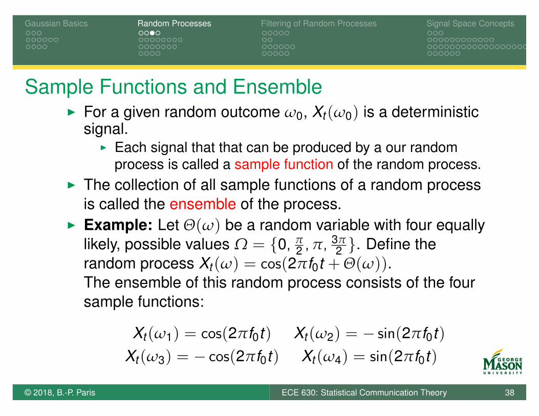
Sample Functions and EnsembleI For a given random outcome w0, Xt (w0) is a deterministic

signal.I Each signal that that can be produced by a our random

process is called a sample function of the random process.I The collection of all sample functions of a random process

is called the ensemble of the process.I Example: Let Q(w) be a random variable with four equally

likely, possible values W = {0, p2 ,p, 3p

2 }. Define therandom process Xt (w) = cos(2pf0t + Q(w)).The ensemble of this random process consists of the foursample functions:

Xt (w1) = cos(2pf0t) Xt (w2) = � sin(2pf0t)Xt (w3) = � cos(2pf0t) Xt (w4) = sin(2pf0t)



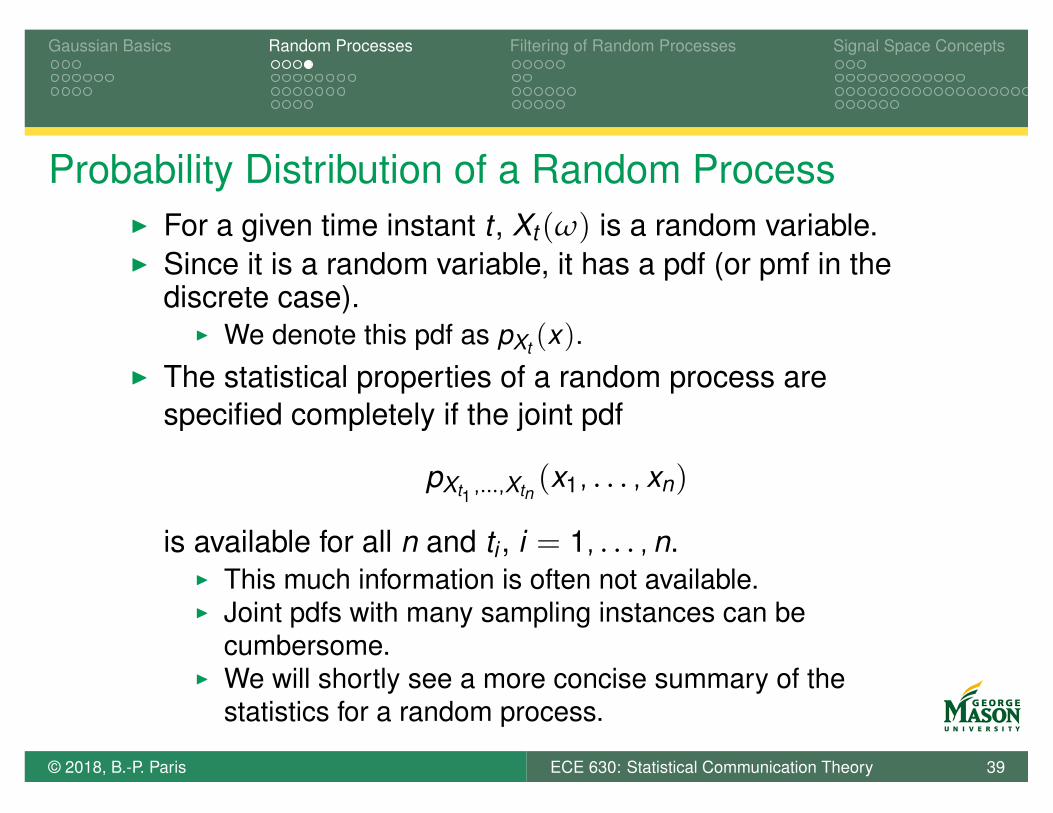
Probability Distribution of a Random ProcessI For a given time instant t , Xt (w) is a random variable.I Since it is a random variable, it has a pdf (or pmf in the

discrete case).I We denote this pdf as pXt (x).

I The statistical properties of a random process arespecified completely if the joint pdf

pXt1 ,...,Xtn(x1, . . . , xn)

is available for all n and ti , i = 1, . . . , n.I This much information is often not available.I Joint pdfs with many sampling instances can be

cumbersome.I We will shortly see a more concise summary of the

statistics for a random process.



Random Process with Random Parameters

I A deterministic signal that depends on a randomparameter is a random process.

I Note, the sample functions of such random processes donot “look” random.

I Running Examples:I Example (discrete phase): Let Q(w) be a random variable

with four equally likely, possible values W = {0, p2 ,p, 3p

2 }.Define the random process Xt (w) = cos(2pf0t + Q(w)).

I Example (continuous phase): same as above but phaseQ(w) is uniformly distributed between 0 and 2p,Q(w) ⇠ U [0, 2p).

I For both of these processes, the complete statisticaldescription of the random process can be found.



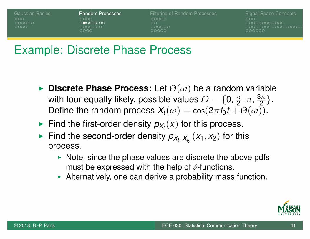
Example: Discrete Phase Process

I Discrete Phase Process: Let Q(w) be a random variablewith four equally likely, possible values W = {0, p

2 ,p, 3p2 }.

Define the random process Xt (w) = cos(2pf0t + Q(w)).I Find the first-order density pXt (x) for this process.I Find the second-order density pXt1 Xt2

(x1, x2) for thisprocess.

I Note, since the phase values are discrete the above pdfsmust be expressed with the help of d-functions.

I Alternatively, one can derive a probability mass function.



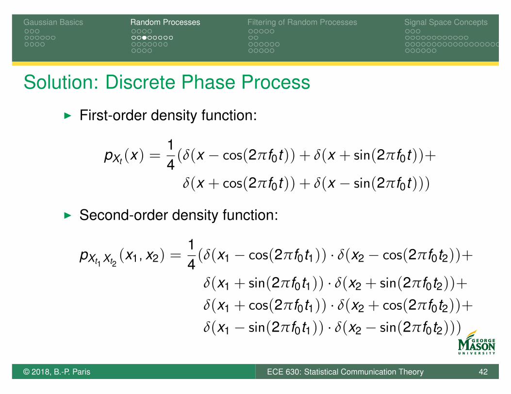
Solution: Discrete Phase ProcessI First-order density function:

pXt (x) =14(d(x � cos(2pf0t)) + d(x + sin(2pf0t))+

d(x + cos(2pf0t)) + d(x � sin(2pf0t)))

I Second-order density function:

pXt1 Xt2(x1, x2) =

14(d(x1 � cos(2pf0t1)) · d(x2 � cos(2pf0t2))+

d(x1 + sin(2pf0t1)) · d(x2 + sin(2pf0t2))+d(x1 + cos(2pf0t1)) · d(x2 + cos(2pf0t2))+d(x1 � sin(2pf0t1)) · d(x2 � sin(2pf0t2)))



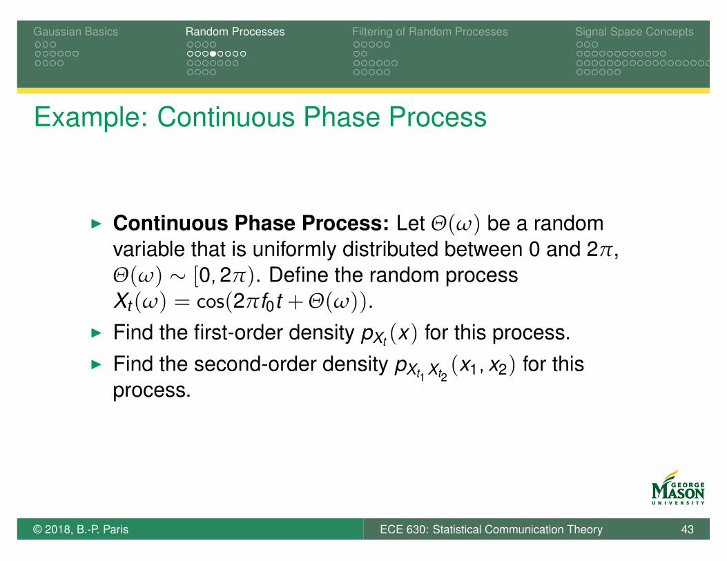
Example: Continuous Phase Process

I Continuous Phase Process: Let Q(w) be a randomvariable that is uniformly distributed between 0 and 2p,Q(w) ⇠ [0, 2p). Define the random processXt (w) = cos(2pf0t + Q(w)).

I Find the first-order density pXt (x) for this process.I Find the second-order density pXt1 Xt2

(x1, x2) for thisprocess.



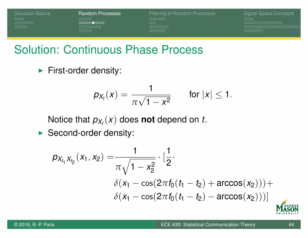
Solution: Continuous Phase ProcessI First-order density:

pXt (x) =1

pp

1 � x2for |x | 1.

Notice that pXt (x) does not depend on t .I Second-order density:

pXt1 Xt2(x1, x2) =

1

pq

1 � x22

· [12·

d(x1 � cos(2pf0(t1 � t2) + arccos(x2)))+

d(x1 � cos(2pf0(t1 � t2)� arccos(x2)))]



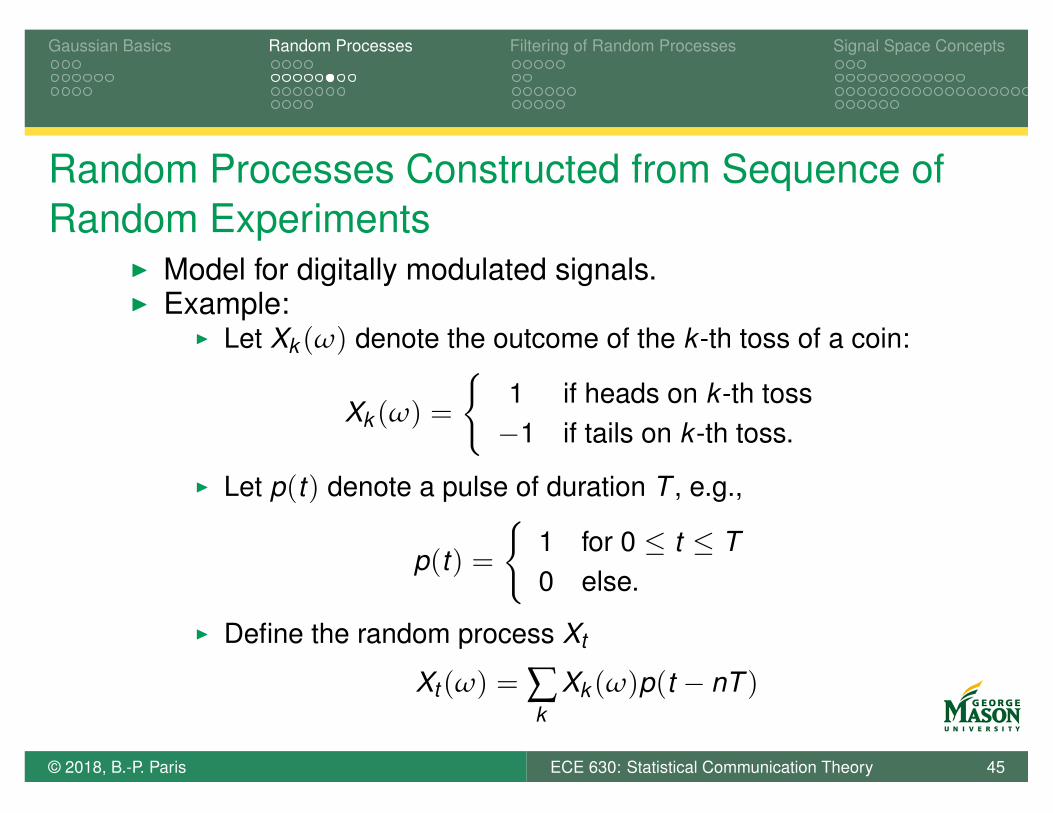
Random Processes Constructed from Sequence ofRandom Experiments

I Model for digitally modulated signals.I Example:

I Let Xk (w) denote the outcome of the k -th toss of a coin:

Xk (w) =

(1 if heads on k -th toss�1 if tails on k -th toss.

I Let p(t) denote a pulse of duration T , e.g.,

p(t) =

(1 for 0 t T0 else.

I Define the random process Xt

Xt (w) = Âk

Xk (w)p(t � nT )



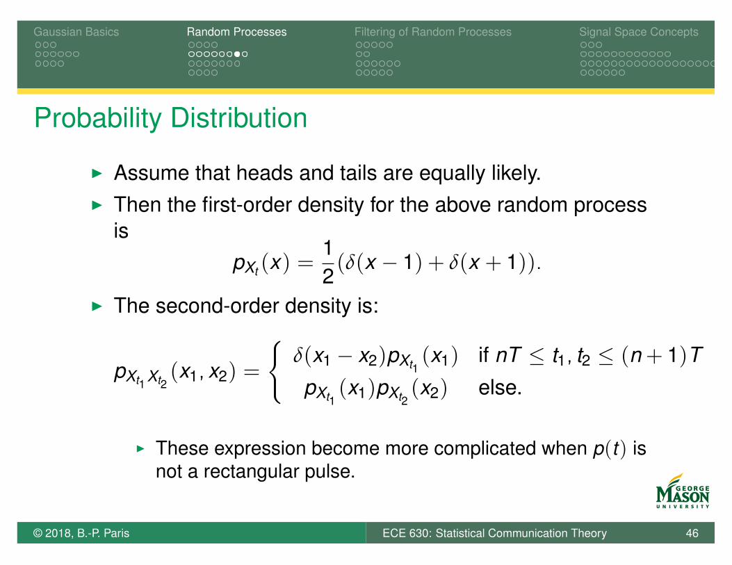
Probability Distribution

I Assume that heads and tails are equally likely.I Then the first-order density for the above random process

ispXt (x) =

12(d(x � 1) + d(x + 1)).

I The second-order density is:

pXt1 Xt2(x1, x2) =

(d(x1 � x2)pXt1

(x1) if nT t1, t2 (n + 1)TpXt1

(x1)pXt2(x2) else.

I These expression become more complicated when p(t) isnot a rectangular pulse.



Probability Density of Random Processs DefinedDirectly

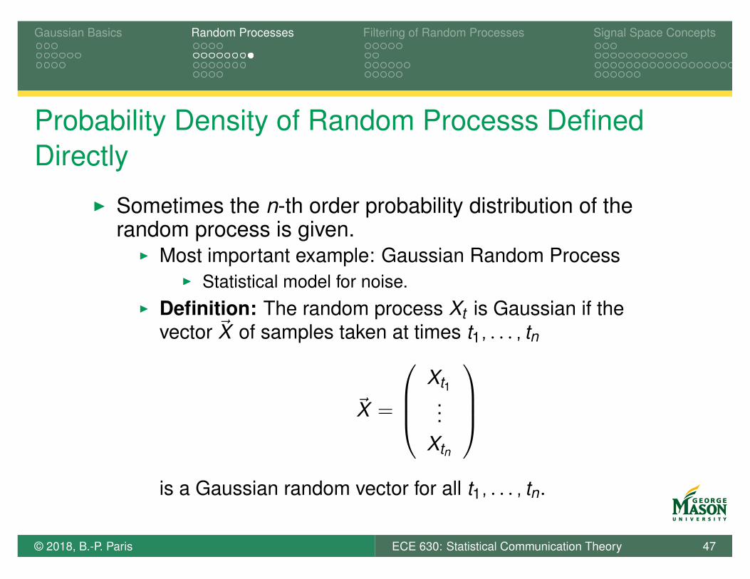
I Sometimes the n-th order probability distribution of therandom process is given.

I Most important example: Gaussian Random ProcessI Statistical model for noise.

I Definition: The random process Xt is Gaussian if thevector ~X of samples taken at times t1, . . . , tn

~X =

0

BB@

Xt1...

Xtn

1

CCA

is a Gaussian random vector for all t1, . . . , tn.



Second Order Description of Random ProcessesI Characterization of random processes in terms of n-th

order densities isI frequently not availableI mathematically cumbersome

I A more tractable, practical alternative description isprovided by the second order description for a randomprocess.

I Definition: The second order description of a randomprocess consists of the

I mean function and theI autocorrelation function

of the process.I Note, the second order description can be computed from

the (second-order) joint density.I The converse is not true — at a minimum the distribution

must be specified (e.g., Gaussian).© 2018, B.-P. Paris ECE 630: Statistical Communication Theory 48


Mean Function

I The second order description of a process relies on themean and autocorrelation functions — these are definedas follows

I Definition: The mean of a random process is defined as:

E[Xt ] = mX (t) =Z •

�•x · pXt (x) dx

I Note, that the mean of a random process is a deterministicsignal.

I The mean is computed from the first oder density function.



Autocorrelation Function

I Definition: The autocorrelation function of a randomprocess is defined as:

RX (t , u) = E[XtXu ] =Z •

�•

Z •

�•xy · pXt ,Xu (x , y) dx dy

I Autocorrelation is computed from second order density



Autocovariance Function

I Closely related: autocovariance function:

CX (t , u) = E[(Xt � mX (t))(Xu � mX (u))]= RX (t , u)� mX (t)mX (u)



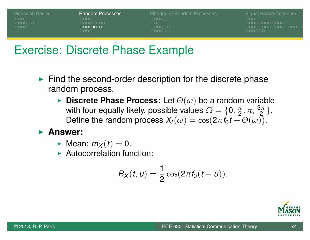
Exercise: Discrete Phase Example

I Find the second-order description for the discrete phaserandom process.

I Discrete Phase Process: Let Q(w) be a random variablewith four equally likely, possible values W = {0, p

2 ,p, 3p2 }.

Define the random process Xt (w) = cos(2pf0t + Q(w)).I Answer:

I Mean: mX (t) = 0.I Autocorrelation function:

RX (t , u) =12cos(2pf0(t � u)).



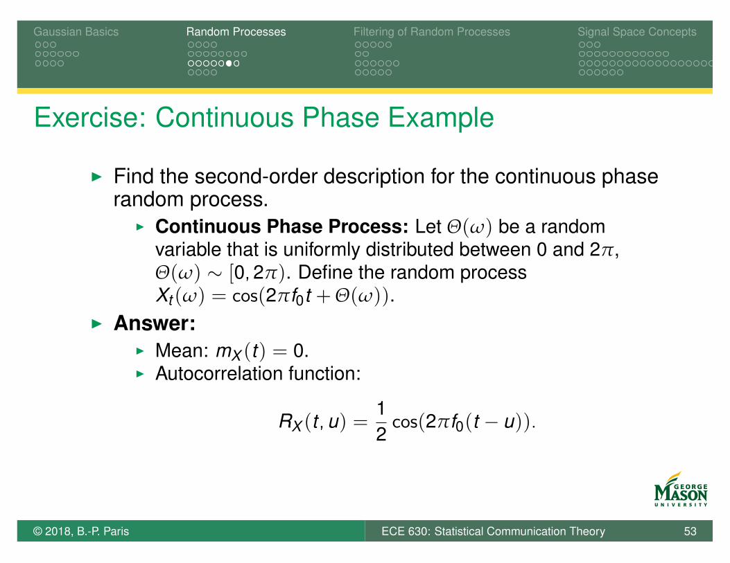
Exercise: Continuous Phase Example

I Find the second-order description for the continuous phaserandom process.

I Continuous Phase Process: Let Q(w) be a randomvariable that is uniformly distributed between 0 and 2p,Q(w) ⇠ [0, 2p). Define the random processXt (w) = cos(2pf0t + Q(w)).

I Answer:

I Mean: mX (t) = 0.I Autocorrelation function:

RX (t , u) =12cos(2pf0(t � u)).



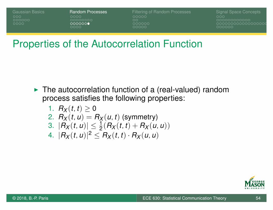
Properties of the Autocorrelation Function

I The autocorrelation function of a (real-valued) randomprocess satisfies the following properties:

1. RX (t , t) � 02. RX (t , u) = RX (u, t) (symmetry)3. |RX (t , u)| 1

2 (RX (t , t) + RX (u, u))4. |RX (t , u)|2 RX (t , t) · RX (u, u)



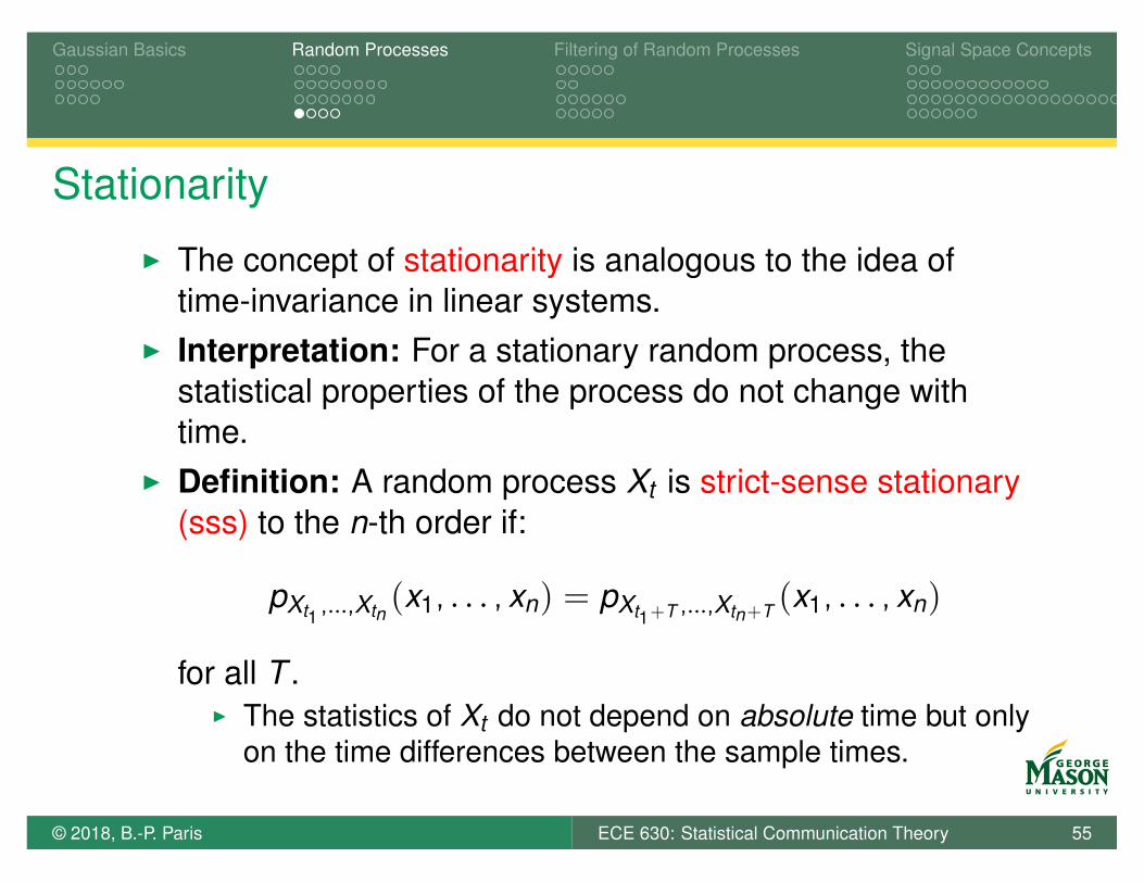
StationarityI The concept of stationarity is analogous to the idea of

time-invariance in linear systems.I Interpretation: For a stationary random process, the

statistical properties of the process do not change withtime.

I Definition: A random process Xt is strict-sense stationary(sss) to the n-th order if:

pXt1 ,...,Xtn(x1, . . . , xn) = pXt1+T ,...,Xtn+T (x1, . . . , xn)

for all T .I The statistics of Xt do not depend on absolute time but only

on the time differences between the sample times.



Wide-Sense Stationarity

I A simpler and more tractable notion of stationarity is basedon the second-order description of a process.

I Definition: A random process Xt is wide-sense stationary(wss) if

1. the mean function mX (t) is constant and

2. the autocorrelation function RX (t , u) depends on t and uonly through t � u, i.e., RX (t , u) = RX (t � u)

I Notation: for a wss random process, we write theautocorrelation function in terms of the singletime-parameter t = t � u:

RX (t , u) = RX (t � u) = RX (t).



Exercise: StationarityI True or False: Every random process that is strict-sense

stationarity to the second order is also wide-sensestationary.

I Answer: TrueI True or False: Every random process that is wide-sense

stationary must be strict-sense stationarity to the secondorder.

I Answer: FalseI True or False: The discrete phase process is strict-sense

stationary.I Answer: False; first order density depends on t , therefore,

not even first-order sss.I True or False: The discrete phase process is wide-sense

stationary.I Answer: True



White Gaussian Noise

I Definition: A (real-valued) random process Xt is calledwhite Gaussian Noise if

I Xt is Gaussian for each time instance tI Mean: mX (t) = 0 for all tI Autocorrelation function: RX (t) =

N02 d(t)

I White Gaussian noise is a good model for noise incommunication systems.

I Note, that the variance of Xt is infinite:

Var(Xt ) = E[X 2t ] = RX (0) =

N02

d(0) = •.

I Also, for t 6= u: E[XtXu ] = RX (t , u) = RX (t � u) = 0.


Documents

Random Processes — Why we Care