Random Recursive Partitioning: a matching method for the

JOURNAL OF APPLIED ECONOMETRICSJ. Appl. Econ. 24: 163–185 (2009)Published online 2 September 2008 in Wiley InterScience(www.interscience.wiley.com) DOI: 10.1002/jae.1026

RANDOM RECURSIVE PARTITIONING: A MATCHINGMETHOD FOR THE ESTIMATION OF THE AVERAGE

TREATMENT EFFECT

GIUSEPPE PORRO1* AND STEFANO MARIA IACUS2

1 Department of Economics and Statistics, University of Trieste, P.le Europa 1, I-34127 Trieste, Italy2 Department of Economics, Business and Statistics, University of Milan, Via Conservatorio 7, I-20122 Milano, Italy

SUMMARYIn this paper we introduce the Random Recursive Partitioning (RRP) matching method. RRP generates aproximity matrix which might be useful in econometric applications like average treatment effect estimation.RRP is a Monte Carlo method that randomly generates non-empty recursive partitions of the data andevaluates the proximity between two observations as the empirical frequency they fall in a same cell of theserandom partitions over all Monte Carlo replications. From the proximity matrix it is possible to derive bothgraphical and analytical tools to evaluate the extent of the common support between data sets. The RRPmethod is “honest” in that it does not match observations “at any cost”: if data sets are separated, the methodclearly states it.

The match obtained with RRP is invariant under monotonic transformation of the data. Average treatmenteffect estimators derived from the proximity matrix seem to be competitive compared to more commonlyused estimators. RRP method does not require a particular structure of the data and for this reason it can beapplied when distances like Mahalanobis or Euclidean are not suitable, in the presence of missing data orwhen the estimated propensity score is too sensitive to model specifications. Copyright 2008 John Wiley& Sons, Ltd.

Received 1 October 2004; Revised 9 February 2007

1. INTRODUCTION

In social as well as in natural sciences researchers often need to estimate the effect of a “treatment”(like a social program, a medical therapy, etc) on a population of individuals. The estimationgenerally entails the comparison of an outcome variable between the group of the subjects exposedto the treatment and a “control” group which did not receive the treatment.

The evaluation of the differential treatment effect on the outcome for treated versus controlindividuals has to be done given the same pre-treatment conditions (see e.g. Heckman et al.,1997, 1998). In experimental studies two similar groups of individuals are randomly selected froma population: one is then exposed to the treatment and the other is not. In observational studiesthe assignment to the treatment is usually non-randomized and, therefore, the distributions of pre-treatment covariates are different between the two groups. Finding control units similar to eachtreated individual represents the preliminary problem of the analysis. Therefore, a technique isrequired for matching observations coming from different data sets. If the match fails partially or

Ł Correspondence to: Professor Giuseppe Porro, Department of Economics and Statistics, University of Trieste, PiazzaleEuropa, 1 Trieste, 34127, Italy. E-mail: [email protected]

Copyright 2008 John Wiley & Sons, Ltd.

164 GIUSEPPE PORRO AND STEFANO M. IACUS

completely, it means that the distributions of the covariates in the two groups do not overlap. Thisis a case of (partial or total) lack of common support (see §2.2 and §2.4).

When there are many covariates the match might become an unfeasible task. Hence, since theseminal paper by Cochran and Rubin (1973), many authors have faced the matching problem andseveral matching techniques have been developed to overcome this dimensionality issue (see alsoRubin 1973a,b). In their paper of 1973, Cochran and Rubin (among other contributions) proposedto solve the problem of multivariate matching using the Mahalanobis distance (Rubin, 1980)by matching the nearest available individuals. Later Rosenbaum and Rubin (1983) introducedthe notion of propensity score (PS) as the probability that an individual receives the treatment,conditional on his/her covariates (see §3.1.3).

Rosenbaum (1989) introduced further the notion of optimal matching that is a matching strategyto group treated and control units in a way that minimizes the overall distance between observations(see §3.2). The drawback of all unconstrained methods based on distances or propensity scores isthat, if two data sets are separated (i.e. they have no common support), a match can always befound among the “less distant” observations, but the achieved matching may be meaningless. Insuch cases, it is more effective the use of a caliper (a bound) on the distance or on the propensityscore or a mix of the two. Rosenbaum and Rubin (1985a, b) and Gu and Rosenbaum (1993) showthe performance of different methods under this setup.

Propensity score matching has been brought back to the attention of the statistical communityafter the work of Dehejia and Whaba (1999). In their paper the authors suggest that propensityscore matching is a good way to reduce bias in the estimation of the average treatment effect inobservational studies (no matter the data sets to be matched). The debate that followed (Dehejia andWhaba 2002, Smith and Todd 2005a, b and Dehejia, 2005) was mainly focused on the sensitivityof the match to the model used to estimate the propensity score. In this respect, different parametricas well as nonparametric procedures (see e.g. Stone et al., 1995, Hirano et al., 2003) to estimatethe propensity score have been proposed.

In this paper we propose a new matching algorithm which is invariant under monotonictransformation of the data. This method, named Random Recursive Partitioning (RRP) does notrely on a particular distance or on a specific model to be estimated and it does not suffer of theproblem of “matching at any cost”. It works on the spatial distribution of the observations andtries to figure out, using Monte Carlo arguments, whether two observations can be consideredequal.

This method generates a proximity (complementarily, a dissimilarity) measure between obser-vations which can be easily interpreted as the belief of two observations to be equal in covariatesin the sense that they lie in the same region of the space (whichever the nature of this space).Information coming from this dissimilarity can be used as both a graphical and numerical toolto examine the extent of the common support between data sets. Once the common support hasbeen identified, the observations in the common support can be used to evaluate the portion of theaverage treatment effect that can be reliably estimated.

The RRP method can in fact be considered an alternative to the matching methods proposedso far in the literature when distributional hypotheses cannot be assumed or when distances, likeMahalanobis, are not appropriate because of the nature of the data. This method, like the GeneticMatching algorithm (Diamond and Sekhon, 2005), is computationally intensive but still fast enoughto be a usable device in applications. A free software ready to use is available for the R statisticalenvironment.

Copyright 2008 John Wiley & Sons, Ltd. J. Appl. Econ. 24: 163–185 (2009)DOI: 10.1002/jae

RANDOM RECURSIVE PARTITIONING 165

The paper is organized as follows: in Section 2 we introduce the Random Recursive Partitioningmethod and discuss the tools for the identification of the common support between data sets. Section3 describes the problem of average treatment effect estimation and presents several alternativeestimators, including the ones derived from the RRP method. In Section 4 our methodology isapplied to the NSW data set analyzed originally in Lalonde (1986) with the aim to compare theRRP-based estimators to their competitors currently available in the literature. Section 5 reportsMonte Carlo evidence of the ability of RRP to reduce the bias in covariates and some results onthe asymptotic bias and limiting distribution of ATT estimators based on RRP.

2. RANDOM RECURSIVE PARTITIONING ALGORITHM

The RRP method is based on regression trees (RT), which recently become quite popular indatamining applications. Briefly, a regression tree (Breiman et al., 1984) models the expectedvalue of some response variable Y conditionally on a set of covariates X D !X1, X2, . . . , Xp"by partitioning the observations on the basis of their covariates. The resulting final partition issuch that in each stratum the homogeneity of the outcome Y is the maximum achievable withrespect to some criterion (e.g. deviance for continuous variates or Gini index for categoricalresponse variable). Starting from the set of complete observations the algorithm explores everypossible bipartite stratification of the observations generated by each covariate Xi and finally splitsthe observations in two subsets according to the stratification to the variable that leads to themaximum homogeneity of the outcome inside both groups: for example, suppose that the variableis Xj, then each observation is moved in one group if for this observation Xj < x and to the othergroup if Xj ½ x (where x is the some optimal splitting threshold identified by RT). Thus, after thefirst iteration two groups are formed. At the second step, for each of the two groups the same ruleis applied and two new groups are generated from each of the former. The algorithm stops whenenough homogeneity in the currently formed groups is reached or when the size of the groupsis small enough. Intermediate subgroups are called nodes and the final nodes are called leaves.The set of all the leaves corresponds to the final stratification of the whole set of observations.At each step the algorithm generates non empty strata and these strata are generated recursively.Optimization is not global as the algorithm uses a one-step look-ahead strategy2. Regression treesare quite effective in describing the dependence of the response variable Y on the covariates Xand their interactions when looking at their graphical representation.

Regression trees have some features that make them interesting in matching applications. Inparticular, the generated partition is invariant under monotonic transformations of the data X (seeBreiman et al., 1984, pag. 57) because the algorithm only considers the order of the values ofeach covariate and not the values themselves (it is essentially the same argument of median versusarithmetic mean). Another interesting feature is that regression trees tends to overfit the data.Overfit is of course not a good feature if the tree is used to predict the response variable Y fornew observations, but in matching applications this is exactly what we desire to have: the resultingpartition tailors the structure of the data. RRP uses the regression trees algorithm only to partitionthe observations and then generates a proximity which turns out to be quite effective in solvingthe matching problem.

2 Other versions of the algorithm have been developed since 1984 for multipartite stratification and global optimizationbut we are not going to use them here.



2.1. The proximity and dissimilarity matrix generated by RRP

The regression trees algorithm needs a response variable, say Z, whose homogeneity has to beoptimized inside the strata. We assign a fictitious response variable to the observations: we draw nrandom numbers zi from the uniform distribution on [0,1] and associate them to the n observationsof the sample.3 So we are going to model Z ¾ !X1, X2, . . . , Xd" where Z is a fictitious responsevariable4 needed to feed the RT algorithm. We then let the RT algorithm grow a tree and obtaina random, recursive and non empty partition of the data. The proximity measure for this randompartition is defined as follows: we set #ij D 1 for all the observations with indexes i and j inthe same leaf and set #ij D 0 otherwise. So we obtain a matrix of 0’s and 1’s, where the 1’scorrespond to observations belonging to the same stratum. The dissimilarity measure is definedas υij D 1 $ #ij. This partition and the dissimilarity/proximity measure entirely depends on thevariable Z: therefore we replicate this procedure R times and at each replication we draw n newrandom numbers zi and grow a new tree. Denote by #!r"

ij the proximity measure for iterationr D 1, . . . , R: the final proposed proximity measure is obtained as the average of the #!r"

ij ’s overthe R replications, i.e.:

RRP D[

#ij D 1R

R∑

rD1

#!r"ij

]

and RRP D 1 $ RRP.

RRP can be seen as a Monte Carlo method on the space of non-empty and recursive partitions of theobservations. We refer to RRP as the RRP-proximity matrix and to RRP as the RRP-dissimilaritymatrix. Please remark that RRP method does not rely on a particular distance but it rather generatesa new dissimilarity measure and, due to the fact that RT algorithm is invariant under monotonictransformations of the data, so is the RRP proximity RRP. Sometimes a preliminary discretizationof continuous covariates is advisable to avoid too wide cells near the border of the support of thedata. In our implementation we suggest to divide the range of each continuous covariate in 15–20intervals. The discretization has also the nice side-effect to reduce the numerical complexity ofour method.

A parameter that controls the size of the leaves generated by the RT algorithm, is the socalled “minsplit” parameter. Setting minsplit D 10 means “split cells with at least 10 observations,otherwise stop”. Empirical evidence and arguments of next section suggest to use very low minsplitvalues (either 5 or 10) for the RRP method.

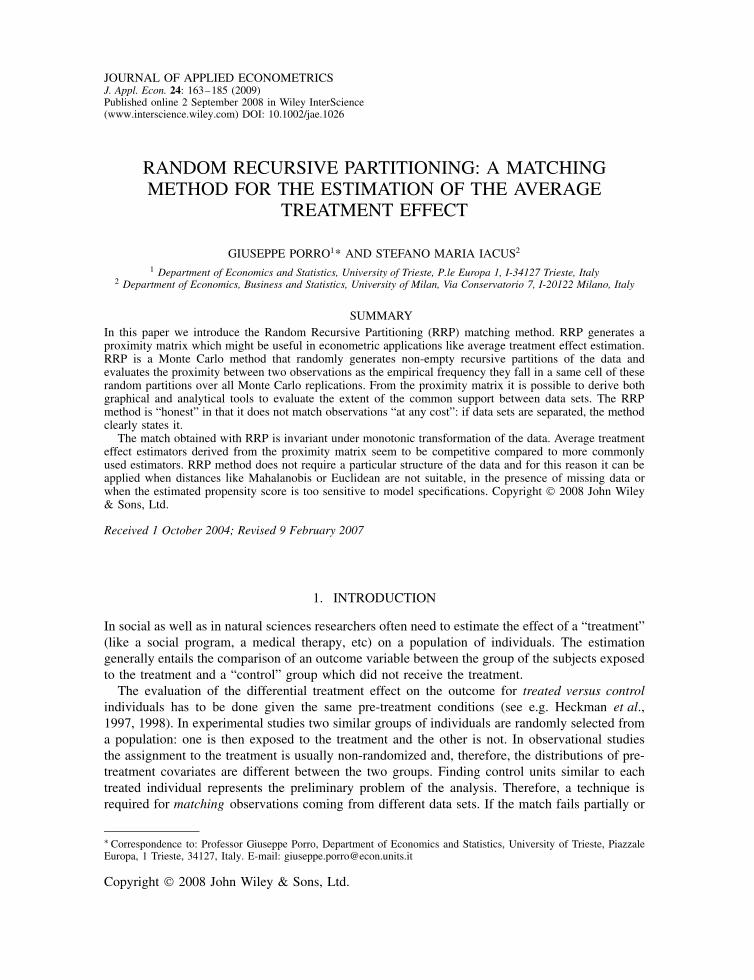
Figure 1 shows some possible partitions generated by the RRP method. That picture clearlyshows that the partitions generated by the RRP algorithm are different from simply slicing the theset of covariates X at random (for example it never generates empty cells). It should also be clearfrom Figure 1 that the “shape” of the data determines the partition.

The RRP method requires, at most, ordering of the variables involved, but works with anykind of data and also in the presence of missing data. So it could be used in matching problemswhenever the use of other well known distances (e.g. Mahalanobis) are debatable.

3 We should notice here that any random assignment which makes observations equally preferable with respect to thisfictitious response variable can be chosen.4 It is to be stressed that this Z variable has nothing to do with the outcome variable of the observational study or withthe treatment. It is just an artifact to run a regression tree.



Figure 1. (UP): two random partitions generated by RRP. (DOWN): the same partitions in the above butwith common support checking in each cell. Data are two multivariate normal samples with same spread anddifferent means. Variables discretized in 15 intervals, minsplit D 8. This figure is available in color online atwww.interscience.wiley.com/journal/jae

2.1.1 About the information coming from the proximity matrixThe RRP method is appreciable in that the elements of matrices RRP and/or RRP can beeasily interpreted. In particular, for some couple of units i and j, υij D 0 means that the twounits always lie in the same cell. Conversely, υij D 1 means that units i and j never fall inthe same cell. In our view it means that these two units should never be matched. It has tobe stressed that RRP is not a distance matrix. Indeed, the proximity #ij can be interpretedonly as the belief of the event “observation i D observation j” to be true, but it gives noinsight about the relative distance between observations. Observations with υij D 1 are simplydifferent but we don’t know how far they are in the space of covariates contrary to what adistance effectively measures. This means that a nearest neighbor approach on RRP it is notlikely to be interesting without replacing υij D 1 with υij D C1. We will discuss this topic in§3.2.



2.2. Preliminary reduction of the data

Prior to attempt a match between different data sets/groups, one should look at the distribution incovariates of the observations in the two groups to figure out if a match makes sense at all. Somegeometric considerations can help to exclude a priori some control units which are likely to beout of the support of the treated units. We report in this section a couple of alternative devices. Inthe applications of §4.2 this preliminary reduction appears to be effective.

2.2.1 Selection via convex hullRecently King and Zeng (2006a, b) proposed to identify the convex hull of one group (say thetreated units) and to exclude from furhter analysis the units from the other group (the controlunits) which do not lie inside this convex hull. The convex hull of the treated units is the smallestsubspace such that, for any two treated units, all points that are on the portion of hyperplaneconnecting them also belong to the subspace. This criterion is quite selective because it excludesfrom the common support all the control units that, although lying out of the convex hull, arenear the treated units which define the boundaries of the convex hull (for further details see citedreferences).

2.2.2 Selection via hyper-rectanglesIn this paper we propose another criterion that consists in constructing the smallest hyper-rectangle which includes all the treated units and to exclude from the analysis all control unitsnot belonging to the hyper-rectangle. This method is less stringent than the convex hull criterionand more easy to implement. Moreover, it does not require any linear structure of the space: itonly requires that, for each covariate, the minimum and maximum can be calculated5. Define!mi, Mi" D !minj2T Xij, maxj2T Xij", i D 1, . . . , p, where T is the set of indexes for the treatedunits and Xij is the value assumed by variable Xi on subject j. The hyper-rectangle is definedby the product H D !m1, M1" ð Ð Ð Ð ð !mp, Mp". Then H corresponds to the region of the spaceX1 ð X2 ð Ð Ð Ð ð Xp which reasonably includes the common support of the two data sets.

2.2.3 About the balance checkThe above methods do not assume any distributional hypotesis which are always hard to be verifiedin real world applications. One the contrary, it does not seem a good idea to use one of such criteriaas a way to check for the balancing property inside the strata to further refine a match.

In fact, virtually any matching algorithm produces a stratification of the data in subgroups.Inside each stratum it might happen that control and treated units are not really homogeneous: tocheck for it, different parametric and nonparametric tests (such as t, Kolmogorov-Smirnov or Chi-Squared tests) are usually applied in the econometric literature. In situations where distributionalhypothesis are hardly verified or when the strata consists of very few observations (like in ourcase) all these tests are likely to be very conservative (for an argument see Becker and Ichino,2002). Conversely, both geometrical methods seem to be too severe and lead to unpleasant resultswhen applied to small cells. We discuss now the drawbacks of the hyper-rectangle approach butsimilar considerations applies to the convex hull method.

5 For non ordinal categorical and dichotomous variables one can take minimum and maximum of coding values withoutaffecting the criterion.



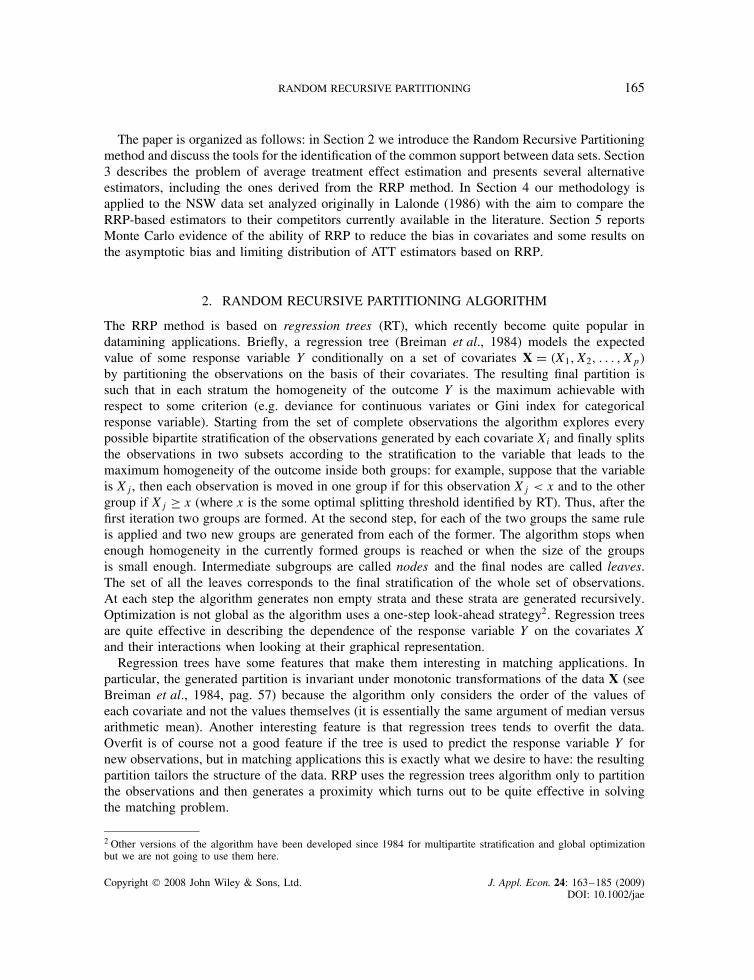
We make use of two-dimensional ad hoc examples for which (given a minsplit value)checking for homogeneity is not efficient whilst a preliminary finer discretization of the sup-port of the covariates would have performed better. In Figure 2 top-left the hyper-rectangleH including the two treated units (full dots) does not contain other control units even ifthey are clearly “close” to the treated ones. The balance check based on the hyper-rectanglethen creates two separate groups and no match between treated and control units can beenobtained. Top-right: for the same data, if we choose a finer discretization of the covari-ates (the dashed line), four cells are created and matching without checking for the bal-ancing property is more reasonable. Figure 2 middle: all controls lie in the hyper-rectagleand hence they are matched, but this is a case where one can see that treated and con-trol units are not homogeneous. Again, a finer discretization gives more reasonable matchbetween treated and control units. Figure 2 bottom shows a case where treated and controlunits are separate on one covariate. In this case the hyper-rectangle gives the correct answerleading to no possible match. However, if we use a finer discretization, the answer remainsunchanged.

So, even if this are peculiar examples, our suggestion is not to use the hyper-rectangle checkand to use instead a small minsplit along with a fine discretization of continuous variables. Thehyper-rectangle as well as the convex hull criterion should probably be used before running anymatching algorithm to roughly select a region which contains the common support between thetreated and control units or, as any other balance check, in the RRP algorithm when strata arecrowded enough. It should be pointed out, anyway, that it is not costless to suppress balancechecking, particularly when a common support between treated and control units does not exists.Indeed, Figure 1 shows two sample partitions obtained with the RRP method. In the upper part theinformation on treatment variable is ignored and hence no balance check inside cells is applied.The lower part of the figure represents the same partition after applying the hyper-rectanglecheck: no cells contain observations of both groups, hence treated and control units have beenseparated.

2.3. EPBR property and the RRP method

Cochran and Rubin (1973) introduced (without naming it) the property of EPBR (Equal PercentBias Reduction) with respect to the Mahalanobis metric saying that ‘‘if x is spherical andsymmetric ( . . .) Mahalanobis distance implies the same percent reduction in bias for each x!k"”. TheEPBR property, formalized later in Rubin (1976a, b), excludes, for example, the unappealing caseof a matching method which is able to reduce the bias on one covariate producing, at the same time,an increase in the bias on some others. Matching methods can also be affinely invariant in the sensethat affine transformations on the covariates lead to the same match of the observations. Under thehypothesis of ellipsoidal distribution on the data—for example multinormal samples—Rubin andThomas (1992a) show that any affinely invariant matching method is also EPBR. As alreadymentioned, RRP is invariant invariant under monotonic transformation of the data and notunder general affine transforms. Still, what follows (see §5) appears to be competitive withMahalanobis matching under conditions for EPBR and sometimes better when these conditionsare not met.



Figure 2. RRP with small minsplit. On the left: with balance check with hyper-rectangles, on the right afiner discretization on continuous variates. In some cases it is better to choose a finer discretization. (Filleddots D treated units, circles D control units)



2.4. The proximity matrix and the identification of the common support

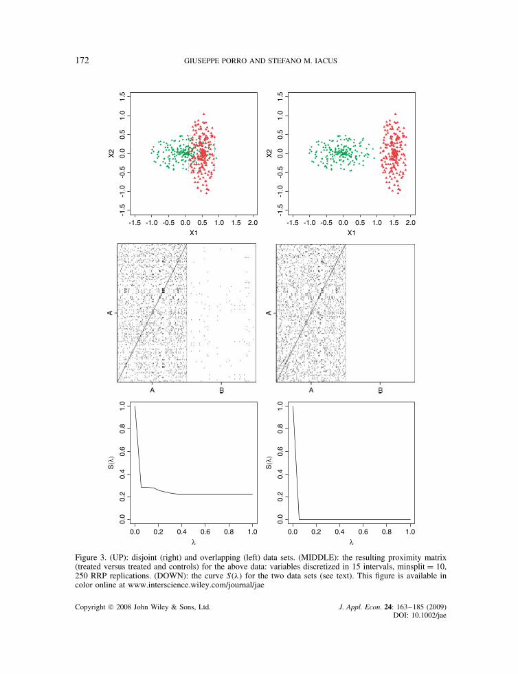
The proximity matrix generated by the RRP method contains insights for the determination of theextent of the common support between two data sets, for example experimental treated individualsT and non experimental controls C. The analysis can be made by a graphical inspection of RRP

and by calculating some related quantities. We illustrate it with a driving example. In Figure 3 twosituations are shown corresponding to two data sets: one with partial common support betweentreated and control individuals (left column) and one with complete absence of a common support(right column). In the first row the two data sets are represented. These data have been randomlygenerated: they are made of 400 units (200 treated, 200 control units). In the second row we plottedthe two RRP’s. In particular, each plot represents the portion of RRP for “treated” (rows) versus“treated and controls” (columns). It is evident that both matrices are dense in the part “treated” vs“treated”. For the non overlapping data set (middle-right) the “treated vs controls” part of RRP

has all #ij D 0 which means that no treated and control units ever fell in the same cell in the 250RRP replications. This is of course the extreme case of complete absence of a common supportand the graphical inspection of the proximity matrix helps in discovering it. This analysis becomesparticularly effective in the case of p ½ 3 covariates where direct plotting of the data is essentiallyunavailable.

For the partial overlapping case (middle-left) only few #ij are strictly positive indicating thatonly subsets of the control and treated groups have common support. In Figure 3 we also depictedthe hyper-rectangle defined in §2.2.2. We remind that this rectangle corresponds to the region ofthe space X1 ð X2 which reasonably includes the common support. In this rectangle we counted62 treated units. A priori these 62 treated units are the ones which can be potentially matchedwith some controls. If one counts the number of dark spots (#ij > 0, i.e. units actually matched)in the plot of the RRP (middle-left), she will find a total of 61 treated units.

2.4.1 The function S!'"Beside the graphical analysis of the RRP proximity matrix, an analytical tool can be derived fromit. This is the curve S!'", ' 2 [0, 1], defined as follows: S!'" D #fi 2 T : maxj2C #ij ½ 'g/nT,where nT is the number of treated units. For fixed ', the function S!'" is the proportion of treatedunits that matched some control units at least ' times over the R replications of the RRP algorithm.Indeed, S!'" is a non increasing function of ' and it rapidly goes to zero if no match is available.This behavior is well represented in Figure 3 where for the non overlapping case the curve justgoes to zero6 as soon as ' > 0. From the graph of the curve S!'" one should notice that the curvestabilizes around some level, say S!'Ł", which is the proportion of treated units that have alwaysbeen matched: these are the units belonging to the common support. We will refer to 'Ł as theempirical threshold in the applications. The empirical threshold can be used to select only thetreated units belonging to the common support.

3. AVERAGE TREATMENT EFFECT ESTIMATION

In the estimation of the average treatment effect (see Rubin, 1974, 1977, 1978), the differentialeffect of the treatment on some outcome variable between treated and control units has to be

6 In the example S!'" D 0 at point ' D 0.05 because we plotted S!'" on the grid 'i D i/20, i D 0, 1, . . . , 20.



-1.5 -1.0 -0.5 0.0 0.5 1.0 1.5 2.0X1

X2

-1.5

-1.0

-0.5

0.0

0.5

1.0

1.5

-1.5 -1.0 -0.5 0.0 0.5 1.0 1.5 2.0

-1.5

-1.0

-0.5

0.0

0.5

1.0

1.5

X1

X2

0.0 0.2 0.4 0.6 0.8 1.0

0.0

0.2

0.4

0.6

0.8

1.0

λ

S(λ

)

0.0 0.2 0.4 0.6 0.8 1.0λ

0.0

0.2

0.4

0.6

0.8

1.0

S(λ

)

Figure 3. (UP): disjoint (right) and overlapping (left) data sets. (MIDDLE): the resulting proximity matrix(treated versus treated and controls) for the above data: variables discretized in 15 intervals, minsplit D 10,250 RRP replications. (DOWN): the curve S!'" for the two data sets (see text). This figure is available incolor online at www.interscience.wiley.com/journal/jae



evaluated given the same pre-treatment conditions. Here is where the matching techniques areapplied. Formally, for individual i D 1, . . . , N, let !YT

i , YCi " denote the two potential outcomes,

YCi being the outcome of individual i when she is not exposed to the treatment and YT

i the outcomeof individual i when he is exposed to the treatment. If both YC

i and YTi were observable, then the

effect of the treatment on i would be simply YTi $ YC

i . The root of the problem is that only oneof the two outcomes is observed whilst the counterfactual is to be estimated.

Often, the object of interest in applications is the average treatment effect on the subpopulation ofthe NT treated subjects (ATT). Let ( be the ATT, then ( can be written as ( D 1

NT

∑i2T!Y

Ti $ YC

i ".As noticed, the first problem in practice is to estimate the unobserved outcome YC

i . The basic ideabehind matching estimators is the following: for each treated unit i, matching estimators imputeto YC

i the average outcome of control individuals similar to the treated i.To ensure that the matching estimators identify and consistently estimate the treatment effects of

interest, it is always assumed that: a) (unconfoundedness) assignment to treatment is independentof the outcome, conditional on the covariates; b) (overlap) the probability of assignment is boundedaway from zero and one (see Rosenbaum and Rubin, 1983). These hypotheses imply the existenceof a common support on pre-treatment covariates between treated and control units.

3.1. ATT estimators and the proximity matrix

It is possible to derive several estimators from RRP or integrate the information coming from thematrix into other estimators. We review some estimators which will be used in the next sections.

3.1.1 The simple RRP-ATT estimatorA simple ATT estimator based on RRP can be defined as follows:

O( D 1nT

∑

i2T

YTi $

∑

j2Ci

fijYCj

D 1nT

∑

i2T

!YTi $ OYC

i " !1"

where Ci D fj 2 C : #ij > 0g and fij D #ij/∑

j2Ci

#ij is the relative frequency of match conditional

to unit i 2 T. This estimator will be denoted simply by RRP in the the tables.

3.1.2 The weighted RRP-ATT estimatorWe can also integrate the information on the common support coming from the RRP into theO( of (1). Indeed, treated units which achieve high frequency of match provide a more reliablecontribution to the estimation of the ATT. This reliability should be reflected by an ATT estimatorin assigning different weights to each treated unit. For instance, we may define the followingset of weights for !YT

i $ OYCi " : #max

i D maxj2Ci

#ij and qi D #maxi /

∑i2T #max

i , where the qi’s are the

normalized version of these weights, i.e.∑

i2T qi D 1. This set of weights, which takes into accountthe maximum number of times treated unit i has been matched to a control unit, is strictly related toour notion of measurement of the common support. We can now define a weighted ATT estimatorQ( as follows:

Q( D∑

i2T

!YTi $ OYC

i "qi !2"



Obviously, estimator in (2) reduces to (1) when qi D 1/nT. This estimator will be denoted byW.RRP in the tables. Other weighted estimators exists in the literature (see e.g. Hirano et al.,2003) but we are not going to implement them here.

3.1.3 Propensity score and RRPRosenbaum and Rubin (1983) introduced the notion of propensity score (PS) as the probabilitythat an individual i receives the treatment conditional on his/her covariates, sometimes denoted byei!X". Of course, two observations with same values of covariates have the same propensity score:hence they propose to match on the basis of e!X". Under the assumptions in Rubin and Thomas(1992a), the PS matching method is affinely invariant and hence EPBR. The erformance of thePS matching under different assumptions on the distribution of the covariates has been examinedin Rubin and Thomas (1992b, 1996).

3.1.4 Nearest neighbor and the RRPA widely used class of estimators is the one of the nearest neighbor estimators. They start byselecting one treated unit and matching it with the “nearest” k controls (NN(k), where k is usually1, 4, 16) and nearest is with respect to some distance or score, for example the Mahalanobisdistance or the propensity score. Then, another treated unit is chosen and matched using the samecriterion. If control units are removed from the set of the controls after matching, the method is saidwithout replacement. In this case, the order the treated units are chosen has an effect on the finalmatch and hence on the ATT estimate. In the applications we will use a match with replacement.Even if it seems natural to define a NN(k) estimator on the RRP dissimilarity matrix, this is areasonable strategy when k D 1 or when υij D 1 is set to C1. In the applications we calculatethe NN(1) and NN(16) on the Mahalanobis distance (MAH(1) and MAH(16) in the tables) and onthe RRP matrix (RRP(1) and RRP(16) respectively) without any modification of the υij in orderto show the difference in performance.

3.2. Optimal matching and RRP

We also show how to use RRP as an alternative dissimilarity matrix or to define a caliper on otherdistance matrices in the optimal matching algorithm. Rosenbaum (1989) introduced the notion ofoptimal matching which, for a given set of observations, a given distance and a set of weights,is a matching strategy that groups treated and control units in a way that minimizes the overalldistance between observations. Given a stratification of ˛ treated units and ˇ controls in groups(i.e. a match of size !˛, ˇ"), under mild assumptions this match might be improved by transformingit into a full match7 (for an extensive account on optimal matching see Rosenbaum, 2002 Ch. 10).Of course, nothing can be stated about which is the best match in general because this notion ofoptimality is strictly related to the distance adopted, as well as to the size (˛, ˇ) of the match.Nevertheless, this method is computationally more efficient then a greedy match (like the nearestneighbor) because it can be transformed into a problem of a “minimum cost flow in a network”(Bertsekas, 1991) for which highly efficient algorithms exist.

7 A full match is a non overlapping stratification in which each treated is matched with at least one control in a stratum orviceversa a control is matched with one or more treated but does not allow for multiple treated versus multiple controlsmatch.



The drawback of this method, as well as of the nearest neighbor method, is that if two data setshave no common support (and without any restrictions) an optimal match can always be found butthis does not guarantee any good property in the estimation of the average treatment effect. In suchcases, it is more effective the use of some restriction. For example, an observation with propensityscore ei!X" should not be matched with another one whose propensity score ej!X" is outside aprescribed radius/caliper r, i.e. if jei!X" $ ej!X"j > r. Rosenbaum and Rubin (1985a) proposed thenearest available Mahalanobis metric matching within calipers defined by the propensity score8 andshowed its good performance. Also, Gu and Rosenbaum (1993) show the empirical performanceof a full match using the same distance. A different caliper can be derived from RRP. We setυij D C1 when υij ½ υŁ, for some value of υŁ 2 [0, 1]. The same restriction can be imposedon the corresponding terms of other distance matrices, like the Mahalanobis. We will use thefollowing notation: MAH(F) for the the optimal full match ATT estimator on the Mahalanobisdistance, MAH C P(F) for the same estimator with propensity score’s caliper on the Mahalanobisdistance, MAH C RRP(F) for the same estimator with calipers on the RRP-dissimilarities, RRP(F)for the ATT estimator based on the optimal full match on RRP and RRP C RRP(F) for the ATTestimator based on the optimal full match on RRP within calipers on the RRP-dissimilarities.

3.2.1 The “selected” RRP-ATT estimatorWe define finally the “selected” RRP estimator (in a simple and a weighted version). This estimatoris built solely on the treated units that have been matched at least 'Ł % times with some othercontrols, where the empirical threshold 'Ł is defined in §2.4.1. Thus the selected RRP estimatordoes not evaluate the global average treatment effect but only the effect restricted to the portionof treated individuals that can be reliably matched. In the tables the estimator will be denoted bySEL.ATT (and W.SEL.ATT for the weighted version).

3.3. Adjustment for difference-in-covariates

Provided we are given a consistent estimator Oµ0!X" of µ0!X" D E!YCjX", we can also adjust theresidual bias for the difference-in-covariates (see e.g. Abadie and Imbens, 2005) obtaining, forexample, the following adjusted version of the simple RRP-ATT estimator in equation (1):

O( 0 D 1nT

∑

i2T

!YTi $ Oµ0!Xi"" $

∑

j2Ci

fij!YCj $ Oµ0!Xj""

!3"

When treated and control units are matched perfectly, i.e. both control and treated units havethe same values in covariates, this bias correction has no effect. If the bias correction for thedifference-in-covariates has a large impact on the ATT estimate, one can presume that the matchhas not been completely successful or the dependence of the outcome on the covariates is highlynon-linear, since even small covariate imbalances lead to very different counterfactual estimates.This adjustment in covariates will be applied to all of the estimators presented so far.

8 The distance between observations are set to C1 if their corresponding propensity score are as far as (or more then)0.6 times the standard deviation of the distribution of the estimated propensity score.



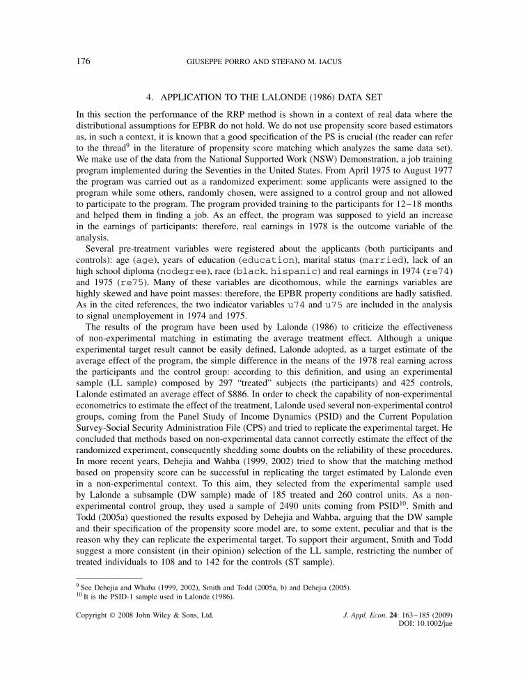
4. APPLICATION TO THE LALONDE (1986) DATA SET

In this section the performance of the RRP method is shown in a context of real data where thedistributional assumptions for EPBR do not hold. We do not use propensity score based estimatorsas, in such a context, it is known that a good specification of the PS is crucial (the reader can referto the thread9 in the literature of propensity score matching which analyzes the same data set).We make use of the data from the National Supported Work (NSW) Demonstration, a job trainingprogram implemented during the Seventies in the United States. From April 1975 to August 1977the program was carried out as a randomized experiment: some applicants were assigned to theprogram while some others, randomly chosen, were assigned to a control group and not allowedto participate to the program. The program provided training to the participants for 12–18 monthsand helped them in finding a job. As an effect, the program was supposed to yield an increasein the earnings of participants: therefore, real earnings in 1978 is the outcome variable of theanalysis.

Several pre-treatment variables were registered about the applicants (both participants andcontrols): age (age), years of education (education), marital status (married), lack of anhigh school diploma (nodegree), race (black, hispanic) and real earnings in 1974 (re74)and 1975 (re75). Many of these variables are dicothomous, while the earnings variables arehighly skewed and have point masses: therefore, the EPBR property conditions are hadly satisfied.As in the cited references, the two indicator variables u74 and u75 are included in the analysisto signal unemployement in 1974 and 1975.

The results of the program have been used by Lalonde (1986) to criticize the effectivenessof non-experimental matching in estimating the average treatment effect. Although a uniqueexperimental target result cannot be easily defined, Lalonde adopted, as a target estimate of theaverage effect of the program, the simple difference in the means of the 1978 real earning acrossthe participants and the control group: according to this definition, and using an experimentalsample (LL sample) composed by 297 “treated” subjects (the participants) and 425 controls,Lalonde estimated an average effect of $886. In order to check the capability of non-experimentaleconometrics to estimate the effect of the treatment, Lalonde used several non-experimental controlgroups, coming from the Panel Study of Income Dynamics (PSID) and the Current PopulationSurvey-Social Security Administration File (CPS) and tried to replicate the experimental target. Heconcluded that methods based on non-experimental data cannot correctly estimate the effect of therandomized experiment, consequently shedding some doubts on the reliability of these procedures.In more recent years, Dehejia and Wahba (1999, 2002) tried to show that the matching methodbased on propensity score can be successful in replicating the target estimated by Lalonde evenin a non-experimental context. To this aim, they selected from the experimental sample usedby Lalonde a subsample (DW sample) made of 185 treated and 260 control units. As a non-experimental control group, they used a sample of 2490 units coming from PSID10. Smith andTodd (2005a) questioned the results exposed by Dehejia and Wahba, arguing that the DW sampleand their specification of the propensity score model are, to some extent, peculiar and that is thereason why they can replicate the experimental target. To support their argument, Smith and Toddsuggest a more consistent (in their opinion) selection of the LL sample, restricting the number oftreated individuals to 108 and to 142 for the controls (ST sample).

9 See Dehejia and Whaba (1999, 2002), Smith and Todd (2005a, b) and Dehejia (2005).10 It is the PSID-1 sample used in Lalonde (1986).



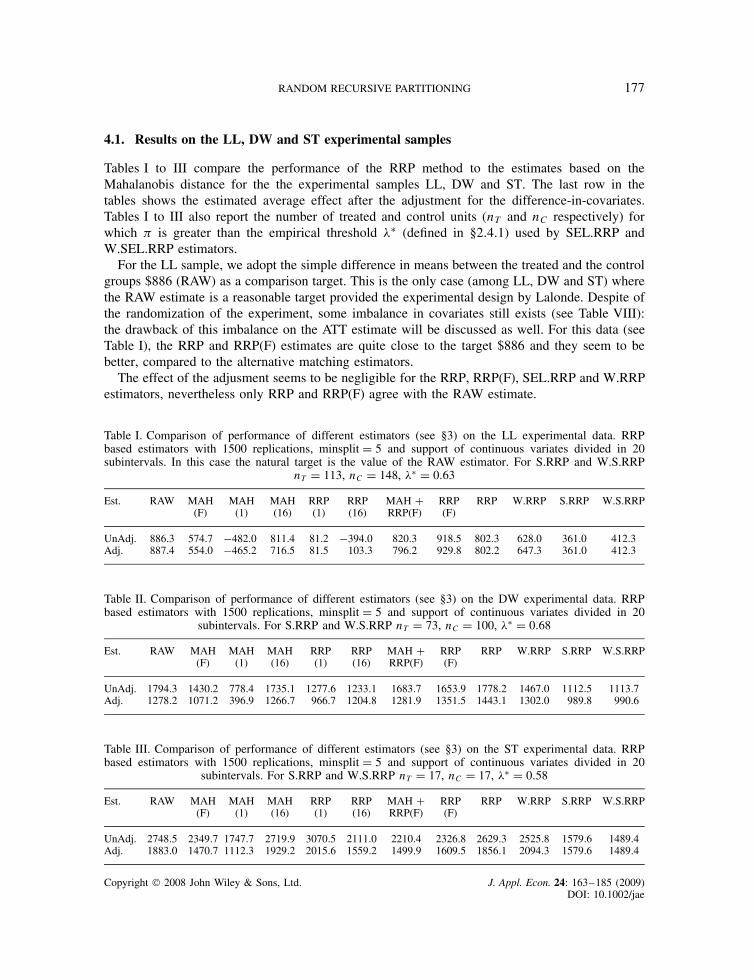
4.1. Results on the LL, DW and ST experimental samples

Tables I to III compare the performance of the RRP method to the estimates based on theMahalanobis distance for the the experimental samples LL, DW and ST. The last row in thetables shows the estimated average effect after the adjustment for the difference-in-covariates.Tables I to III also report the number of treated and control units (nT and nC respectively) forwhich # is greater than the empirical threshold 'Ł (defined in §2.4.1) used by SEL.RRP andW.SEL.RRP estimators.

For the LL sample, we adopt the simple difference in means between the treated and the controlgroups $886 (RAW) as a comparison target. This is the only case (among LL, DW and ST) wherethe RAW estimate is a reasonable target provided the experimental design by Lalonde. Despite ofthe randomization of the experiment, some imbalance in covariates still exists (see Table VIII):the drawback of this imbalance on the ATT estimate will be discussed as well. For this data (seeTable I), the RRP and RRP(F) estimates are quite close to the target $886 and they seem to bebetter, compared to the alternative matching estimators.

The effect of the adjusment seems to be negligible for the RRP, RRP(F), SEL.RRP and W.RRPestimators, nevertheless only RRP and RRP(F) agree with the RAW estimate.

Table I. Comparison of performance of different estimators (see §3) on the LL experimental data. RRPbased estimators with 1500 replications, minsplit D 5 and support of continuous variates divided in 20subintervals. In this case the natural target is the value of the RAW estimator. For S.RRP and W.S.RRP

nT D 113, nC D 148, 'Ł D 0.63

Est. RAW MAH(F)

MAH(1)

MAH(16)

RRP(1)

RRP(16)

MAH CRRP(F)

RRP(F)

RRP W.RRP S.RRP W.S.RRP

UnAdj. 886.3 574.7 $482.0 811.4 81.2 $394.0 820.3 918.5 802.3 628.0 361.0 412.3Adj. 887.4 554.0 $465.2 716.5 81.5 103.3 796.2 929.8 802.2 647.3 361.0 412.3

Table II. Comparison of performance of different estimators (see §3) on the DW experimental data. RRPbased estimators with 1500 replications, minsplit D 5 and support of continuous variates divided in 20

subintervals. For S.RRP and W.S.RRP nT D 73, nC D 100, 'Ł D 0.68

Est. RAW MAH(F)

MAH(1)

MAH(16)

RRP(1)

RRP(16)

MAH CRRP(F)

RRP(F)


UnAdj. 1794.3 1430.2 778.4 1735.1 1277.6 1233.1 1683.7 1653.9 1778.2 1467.0 1112.5 1113.7Adj. 1278.2 1071.2 396.9 1266.7 966.7 1204.8 1281.9 1351.5 1443.1 1302.0 989.8 990.6

Table III. Comparison of performance of different estimators (see §3) on the ST experimental data. RRPbased estimators with 1500 replications, minsplit D 5 and support of continuous variates divided in 20

subintervals. For S.RRP and W.S.RRP nT D 17, nC D 17, 'Ł D 0.58

Est. RAW MAH(F)

MAH(1)

MAH(16)

RRP(1)

RRP(16)

MAH CRRP(F)

RRP(F)


UnAdj. 2748.5 2349.7 1747.7 2719.9 3070.5 2111.0 2210.4 2326.8 2629.3 2525.8 1579.6 1489.4Adj. 1883.0 1470.7 1112.3 1929.2 2015.6 1559.2 1499.9 1609.5 1856.1 2094.3 1579.6 1489.4



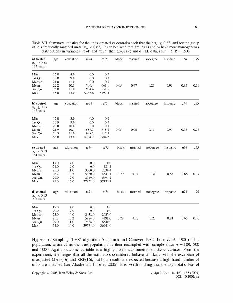
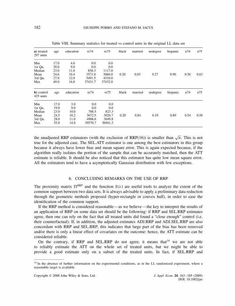
In fact, the distributions of continuous variables in the original LL sample (see Table VIII)indicates that treated and control units have a common support (in terms of range) but thedistribution of their continuous covariates are quite different in shape (see the correspondingquantiles). The SEL.RRP estimator (see §3.2.1) evaluates the average treatment effect restrictedto the treated and control units (groups “a)” and “b)” in Table VII) which, besides belongingto the common support, have also quite similar distribution of continuous covariates. Table VIIcontains the summary statistics for the groups of treated units “a)” and control units “b)” suchthat the corresponding #ij ½ 'Ł D 0.63 and the statistics for less frequently matched treatedunits “c)” and controls “d)”. A reduced dissimilarity can be noted on the distribution of earn-ings (re74 and re75) of treated and control units frequently matched, compared to whathappens on the complementary set and on the whole LL sample (see Table VIII)11. On onehand, this is an evidence of the reliability of the RRP method; on the other hand, it maylead to wonder about which is the real ATT of the Lalonde experiment. What we noticed, infact, is that when the average effect is evaluated with the RRP estimator (therefore includ-ing all treated units in the estimation) we obtain results that are closer to the target adoptedby Lalonde. On the contrary, when we take into account that the two samples do have dif-ferent distribution of continuous covariates and restrict the estimation to the “closest” treatedunits (less than 40%) and controls (about 35%), we obtain different estimates (SEL.RRP)which should be considered reliable for the portion of the phenomenon included in the esti-mation.

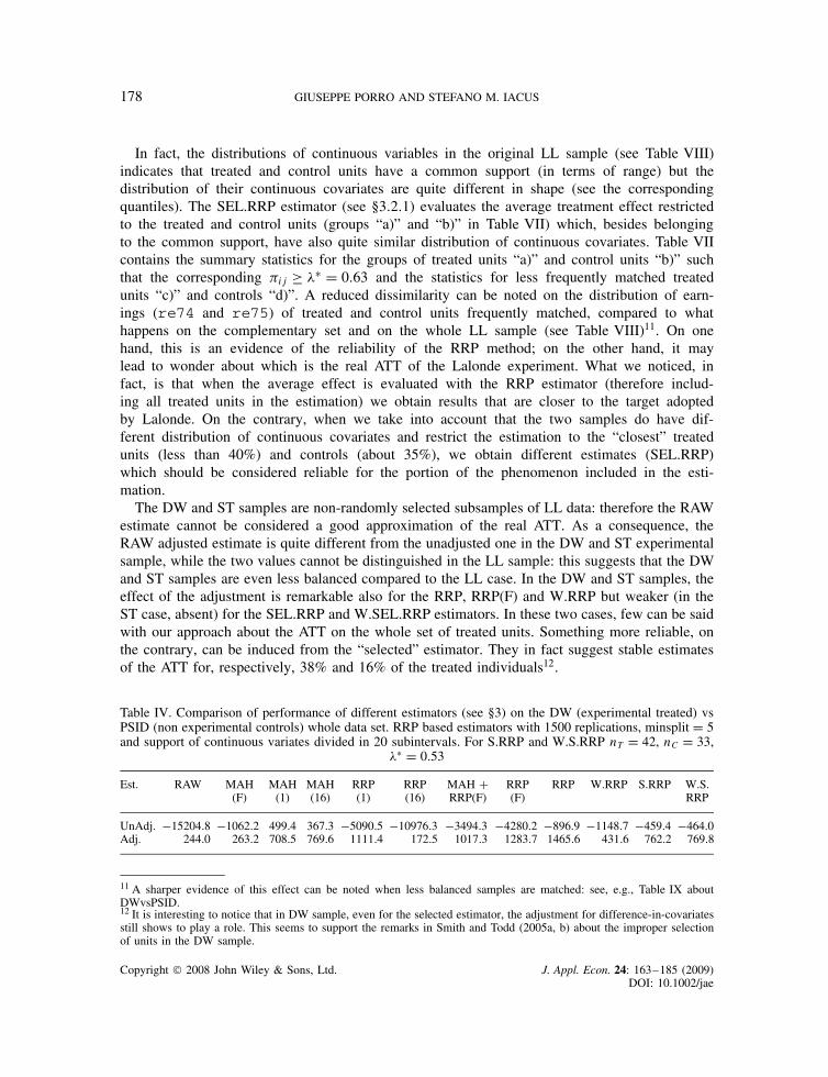
The DW and ST samples are non-randomly selected subsamples of LL data: therefore the RAWestimate cannot be considered a good approximation of the real ATT. As a consequence, theRAW adjusted estimate is quite different from the unadjusted one in the DW and ST experimentalsample, while the two values cannot be distinguished in the LL sample: this suggests that the DWand ST samples are even less balanced compared to the LL case. In the DW and ST samples, theeffect of the adjustment is remarkable also for the RRP, RRP(F) and W.RRP but weaker (in theST case, absent) for the SEL.RRP and W.SEL.RRP estimators. In these two cases, few can be saidwith our approach about the ATT on the whole set of treated units. Something more reliable, onthe contrary, can be induced from the “selected” estimator. They in fact suggest stable estimatesof the ATT for, respectively, 38% and 16% of the treated individuals12.

Table IV. Comparison of performance of different estimators (see §3) on the DW (experimental treated) vsPSID (non experimental controls) whole data set. RRP based estimators with 1500 replications, minsplit D 5and support of continuous variates divided in 20 subintervals. For S.RRP and W.S.RRP nT D 42, nC D 33,

'Ł D 0.53

Est. RAW MAH(F)

MAH(1)

MAH(16)

RRP(1)

RRP(16)

MAH CRRP(F)

RRP(F)


UnAdj. $15204.8 $1062.2 499.4 367.3 $5090.5 $10976.3 $3494.3 $4280.2 $896.9 $1148.7 $459.4 $464.0Adj. 244.0 263.2 708.5 769.6 1111.4 172.5 1017.3 1283.7 1465.6 431.6 762.2 769.8

11 A sharper evidence of this effect can be noted when less balanced samples are matched: see, e.g., Table IX aboutDWvsPSID.12 It is interesting to notice that in DW sample, even for the selected estimator, the adjustment for difference-in-covariatesstill shows to play a role. This seems to support the remarks in Smith and Todd (2005a, b) about the improper selectionof units in the DW sample.



4.2. Results on DW vs PSID non-experimental data

If a non experimental sample is used as a control group, generally the experimental target cannotbe replicated: both Lalonde (1986) and Smith and Todd (2005a) show it by matching the DWexperimental sample to the so called PSID-1 sample, composed by 2490 individuals drawn from thePanel Study of Income Dynamics. Smith and Todd (2005a) argued that, even if match is attained,the average treatment effect cannot be correctly estimated when treated and control samples comefrom different contexts. In this particulat case of DW versus PSID the different context is the locallabour market, therefore, even if a common support between treated and control units were found,one cannot expect to replicate the raw target ($1794) of the DW experimental data. Table IVreports the ATT estimates obtained using the whole PSID-1 sample as the control group. Notice,first of all, that the adjusted estimates strongly differ from the unadjusted ones for all the appliedestimators: this indicates the strong imbalance in covariates that survives the matching. The “raw”unadjusted ATT estimate is a negative quantity, reflecting the higher average earnings level ofthe non-experimental controls, compared to the earnings of the treated individuals. Almost all theestimators fail in replicating the “raw” DW experimental target and the estimates show a largevariability across the estimators.

The selected (and weighted selected) RRP estimators consider only 23% of the treated units(and less than 2% of the controls): Table IX shows that the covariates of treated and controlunits with #ij ½ 0.53 are much more balanced compared to the complementary groups. Despiteof the selection, however, a large correction of the estimates is brought by the adjustment for thedifference in covariates.

Previous results suggest a lack of common support between the two samples. The suspectcan be verified evaluating how many controls are included in the portion of the space ofcovariates where the treated units lie. We consider the two preliminary data reductions presentedin §2.2 based on the convex hull and hyper-rectangle. The hyper-rectangle criterion selects1479 out of 2490 non experimental PSID controls. Table V shows the results of the ATTestimation: the remarkable difference between the adjusted and the unadjusted estimates is stillobservable and all the estimators fail to get the “raw” target. The convex hull criterion, whichis even more selective, selects only 45 out of 2490 control units from the PSID data set.Nevertheless, this does not improve the performance of the ATT estimators very much (seeTable VI).

It is worth noting what happens with the SEL.RRP and W.SEL.RRP estimators: only smallsubsamples of treated and untreated units are involved in both the hyper-rectangle and the convexhull case. The slight differences in the composition of the subsamples are enough to generate largedifferences in the estimated ATT: this can be explained by the non-linear effect of the covariates

Table V. Comparison of performance of different estimators (see §3) on the DW (experimental treated) vsPSID (non experimental controls) reduced to the hyper-rectangle common support (from 2490 to 1479 nonexperimental controls). RRP based estimators with 1500 replications, minsplit D 5 and support of continuous

variates divided in 20 subintervals. For S.RRP and W.S.RRP nT D 19, nC D 11, 'Ł D 0.58

Est. RAW MAH(F)

MAH(1)

MAH(16)

RRP(1)

RRP(16)

MAH CRRP(F)

RRP(F)


UnAdj. $10295.1 $626.9 99.9 666.6 $7.0 $2933.1 $1781.8 $3099.8 $449.6 $563.7 3277.3 3277.3Adj. 165.0 61.9 117.3 848.7 351.9 808.3 630.5 1514.9 859.0 1267.6 3277.3 3277.3



Table VI. Comparison of performance of different estimators (see §3) on the DW (experimental treated)vs PSID (non experimental controls) reduced to the convex-hull common support (from 2490 to 45 nonexperimental controls). RRP based estimators with 1500 replications, minsplit D 5 and support of continuous

variates divided in 20 subintervals. For S.RRP and W.S.RRP nT D 21, nC D 12, 'Ł D 0.47

Est. RAW MAH(F)

MAH(1)

MAH(16)

RRP(1)

RRP(16)

MAH CRRP(F)

RRP(F)


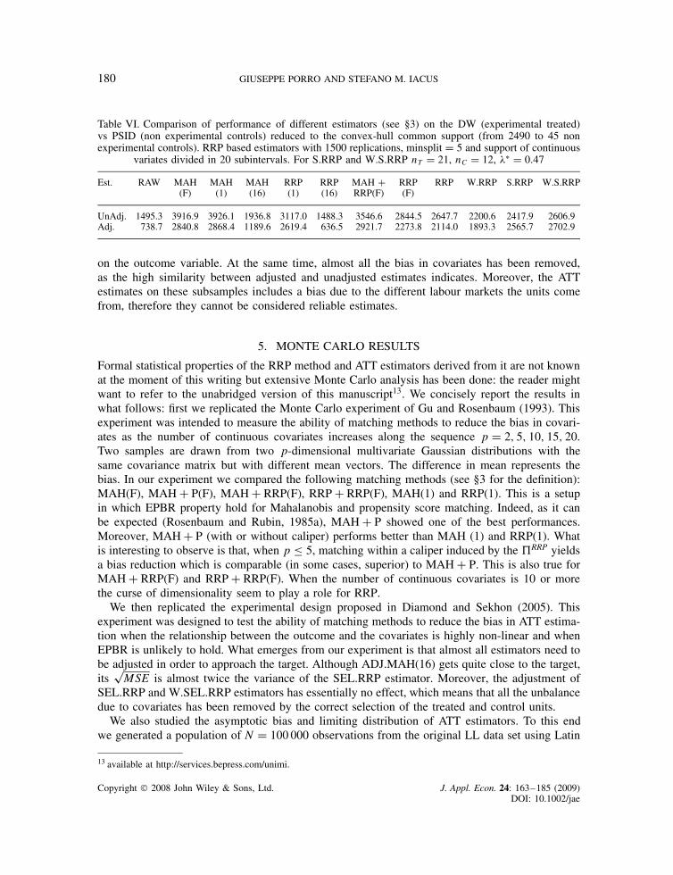
UnAdj. 1495.3 3916.9 3926.1 1936.8 3117.0 1488.3 3546.6 2844.5 2647.7 2200.6 2417.9 2606.9Adj. 738.7 2840.8 2868.4 1189.6 2619.4 636.5 2921.7 2273.8 2114.0 1893.3 2565.7 2702.9

on the outcome variable. At the same time, almost all the bias in covariates has been removed,as the high similarity between adjusted and unadjusted estimates indicates. Moreover, the ATTestimates on these subsamples includes a bias due to the different labour markets the units comefrom, therefore they cannot be considered reliable estimates.

5. MONTE CARLO RESULTS

Formal statistical properties of the RRP method and ATT estimators derived from it are not knownat the moment of this writing but extensive Monte Carlo analysis has been done: the reader mightwant to refer to the unabridged version of this manuscript13. We concisely report the results inwhat follows: first we replicated the Monte Carlo experiment of Gu and Rosenbaum (1993). Thisexperiment was intended to measure the ability of matching methods to reduce the bias in covari-ates as the number of continuous covariates increases along the sequence p D 2, 5, 10, 15, 20.Two samples are drawn from two p-dimensional multivariate Gaussian distributions with thesame covariance matrix but with different mean vectors. The difference in mean represents thebias. In our experiment we compared the following matching methods (see §3 for the definition):MAH(F), MAH C P(F), MAH C RRP(F), RRP C RRP(F), MAH(1) and RRP(1). This is a setupin which EPBR property hold for Mahalanobis and propensity score matching. Indeed, as it canbe expected (Rosenbaum and Rubin, 1985a), MAH C P showed one of the best performances.Moreover, MAH C P (with or without caliper) performs better than MAH (1) and RRP(1). Whatis interesting to observe is that, when p ' 5, matching within a caliper induced by the RRP yieldsa bias reduction which is comparable (in some cases, superior) to MAH C P. This is also true forMAH C RRP(F) and RRP C RRP(F). When the number of continuous covariates is 10 or morethe curse of dimensionality seem to play a role for RRP.

We then replicated the experimental design proposed in Diamond and Sekhon (2005). Thisexperiment was designed to test the ability of matching methods to reduce the bias in ATT estima-tion when the relationship between the outcome and the covariates is highly non-linear and whenEPBR is unlikely to hold. What emerges from our experiment is that almost all estimators need tobe adjusted in order to approach the target. Although ADJ.MAH(16) gets quite close to the target,its

pMSE is almost twice the variance of the SEL.RRP estimator. Moreover, the adjustment of

SEL.RRP and W.SEL.RRP estimators has essentially no effect, which means that all the unbalancedue to covariates has been removed by the correct selection of the treated and control units.

We also studied the asymptotic bias and limiting distribution of ATT estimators. To this endwe generated a population of N D 100 000 observations from the original LL data set using Latin

13 available at http://services.bepress.com/unimi.



Table VII. Summary statistics for the units (treated vs controls) such that their #ij ½ 0.63, and for the groupof less frequently matched units (#ij < 0.63). It can bee seen that groups a) and b) have more homogeneous

distributions in variables ‘re74’ and ‘re75’ then groups c) and d). LL data, split D 5, R D 1500

a) treated#ij ½ 0.63113 units

age education re74 re75 black married nodegree hispanic u74 u75

Min 17.0 4.0 0.0 0.01st Qu. 18.0 9.0 0.0 0.0Median 21.0 11.0 0.0 0.0Mean 22.2 10.3 706.4 661.1 0.05 0.97 0.21 0.96 0.35 0.393rd Qu. 25.0 11.0 934.4 851.6Max 48.0 13.0 9266.6 8497.4

b) control#ij ½ 0.63148 units



c) treated#ij < 0.63184 units



d) control#ij < 0.63277 units



Hypercube Sampling (LHS) algorithm (see Iman and Conover 1982, Iman et al., 1980). Thispopulation, assumed as the true population, is then resampled with sample sizes n D 100, 500and 1000. Again, outcome variable is a highly non-linear function of the covariates. From theexperiment, it emerges that all the estimators considered behave similarly with the exception ofunadjusted MAH(16) and RRP(16), but both results are expected because a high fixed number ofunits are matched (see Abadie and Imbens, 2005). It is worth nothing that the asymptotic bias of



Table VIII. Summary statistics for treated vs control units in the original LL data set

a) treated297 units



b) control425 units



the unadjusted RRP estimators (with the exclusion of RRP(16)) is smaller thanp

n. This is nottrue for the adjusted case. The SEL.ATT estimator is one among the best estimators in this groupbecause it always have lower bias and mean square error. This is again expected because, if thealgorithm really isolates the portion of the sample that can be accurately matched, then the ATTestimate is reliable. It should be also noticed that this estimator has quite low mean square error.All the estimators tend to have a asymptotically Gaussian distribution with few exceptions.

6. CONCLUDING REMARKS ON THE USE OF RRP

The proximity matrix RRP and the function S!'" are useful tools to analyze the extent of thecommon support between two data sets. It is always advisable to apply a preliminary data reductionthrough the geometric methods proposed (hyper-rectangle or convex hull), in order to ease theidentification of the common support.

If the RRP method is considered reasonable—as we believe—the key to interpret the results ofan application of RRP on some data set should be the following: if RRP and SEL.RRP estimatesagree, then one can rely on the fact that all treated units did found a “close enough” control (i.e.their counterfactual). If, in addition, the adjusted estimates ADJ.RRP and ADJ.SEL.RRP are alsoconcordant with RRP and SEL.RRP, this indicates that large part of the bias has been removedand/or there is only a linear effect of covariates on the outcome: hence, the ATT estimate can beconsidered reliable.

On the contrary, if RRP and SEL.RRP do not agree, it means that14 we are not ableto reliably estimate the ATT on the whole set of treated units, but we might be able toprovide a good estimate only on a subset of the treated units. In fact, if SEL.RRP and

14 In the absence of further information on the experimental conditions, as in the LL randomized experiment, where areasonable target is available.



Table IX. Summary statistics for the units (treated vs controls) such that their #ij ½ 0.53, and for the groupof less frequently matched units (#ij < 0.53). It can bee seen that groups a) and b) have more homogeneous

distributions then groups c) and d). DWvsPSID data, split D 5, R D 1500

a) treated#ij ½ 0.5342 units



b) control#ij ½ 0.5333 units



c) treated#ij < 0.53143 units



d) control#ij < 0.532457 units



ADJ.SEL.RRP do agree, then we can state that this is a reliable estimate15 of the “restricted”ATT.

If none of the above is true, i.e. RRP D SEL.RRP and also the adjustment has large effects, noreliable ATT estimate can be drawn from RRP method.

15 Unless there is a confounding factor (e.g. the “labour market” factor in the DW vs PSID application).



The RRP procedure is computationally intensive but, being a Monte Carlo method, it can beeasily parallelized and a ready-to-use software has been written for the R statistical environment(see R Development Core Team, 2005) in the form of a package named rrp and available athttp://CRAN.R-project.org.

ACKNOWLEDGMENTS

We are grateful to two anonimous referees and the A.E. John Rust for careful reading of themanuscript. Their criticism and suggestions have been very elucidating and ended up in a deeplyrevised version of the first manuscript.

REFERENCES

Abadie A, Imbens G. 2005. Large sample properties of matching estimators for average treatment effects,Econometrica , 74(1): 235–267.

Becker S, Ichino A. 2002. Estimation of Average Treatment Effects Based on Propensity Scores, The StataJournal , 2(4): 358–377.

Bertsekas D. 1991. Linear network optimization: algorithm and codes, Cambridge, MA: MIT Press.Breiman L, Friedman JH, Olshen RA, Stone CJ. 1984. Classification and Regression Trees, Monterey,

Wadsworth and Brooks-Cole.Cochran W, Rubin DB. 1973. Controlling Bias in Observational Studies: A Review, Sankhya A, 35: 417–446.Dehejia R. 2005. Practical propensity score matching: a reply to Smith and Todd, Journal of Econometrics ,

125(1–2): 355–364.Dehejia R, Wahba S. 1999. Causal Effects in Nonexperimental Studies: Reevaluating the Evaluation of

Training Programs, Journal of the American Statistical Association , 94: 1053–1062.Dehejia R, Wahba S. 2002. Propensity score matching methods for Non-experimental causal studies, Review

of Economics and Statistics , 84(1): 151–161.Diamond A, Sekhon JS. 2005. Genetic Matching for Estimating Causal Effects: A General Multivariate

Matching Method for Achieving Balance in Observational Studies. Mimeo, available at http://sekhon.polisci.berkeley.edu/papers/GenMatch.pdf.

Gu XS, Rosenbaum PR. 1993. Comparison of multivariates matching methods: structures, distances andalgorithms, Journal of Computational and Graphical Statistics , 2: 405–420.

Heckman J, Ichimura H, Todd P. 1997. Matching as econometric evaluation estimator: evidence fromevaluating a job training programme, Review of Economic Studies , 64(4): 605–654.

Heckman J, Ichimura H, Smith J, Todd P. 1998. Characterizing selection bias using experimental data,Econometrica , 66(5): 1017–1098.

Hirano K, Imbens G, Ridder G. 2003. Efficient Estimation of Average Treatment Effects using the EstimatedPropensity Score, Econometrica , 71: 1161–1189.

Iman RL, Conover WJ. 1982. A distribution-free approach to inducing rank correlation among input variables,Communications in Statistics , B11: 311–334.

Iman RL, Davenport JM, Zeigler DK. 1980. Latin Hypercube Sampling (Program User’s Guide),SAND79 –1473.

King G, Zeng L. 2006a. The Dangers of Extreme Counterfactuals, Political Analysis , 14(2): 131–159.King G, Zeng L. 2006b. When Can History Be Our Guide? The Pitfalls of Counterfactual Inference,

International Studies Quarterly , forthcoming. Available at http://gking.harvard.edu.Lalonde R. 1986. Evaluating the Econometric Evaluations of Training Programs, American Economic Review ,

76: 604–620.R Development Core Team 2005. R: A language and environment for statistical computing. R Foundation

for Statistical Computing, Vienna, Austria. ISBN 3-900051-07-0. Software available at http://www.R-project.org.

Rosenbaum PR. 1989. Optimal matching in observational studies, Journal of the American StatisticalAssociation , 84: 1024–1032.



Rosenbaum PR. 2002. Observational studies, Second Edition, Springer-Verlag: New York.Rosenbaum PR, Rubin DB. 1983. The Central Role of the Propensity Score in Observational Studies for

Causal Effects, Biometrika , 70: 41–55.Rosenbaum PR, Rubin DB. 1985a. Constructing a Control Group Using Multivariate Matched Sampling

Methods That Incorporate the Propensity Score, The American Statistician , 39: 33–38.Rosenbaum PR, Rubin DB. 1985b. The Bias Due to Incomplete Matching, Biometrics , 41: 103–116.Rubin DB. 1973a. The Use of Matched Sampling and Regression Adjustment to Remove Bias in Observa-

tional Studies, Biometrics , 29: 185–203.Rubin DB. 1973b. Matching to Remove Bias in Observational Studies, Biometrics , 29: 159–183.Rubin DB. 1974. Estimating Causal Effects of Treatments in Randomized and non-randomized Studies,

Journal of Educational Psychology , 66: 688–701.Rubin DB. 1976a. Multivariate Matching Methods That are Equal Percent Bias Reducing, I: Some Examples,

Biometrics , 32: 109–120.Rubin DB. 1976b. Multivariate Matching Methods That are Equal Percent Bias Reducing, II: Maximums on

Bias Reduction for Fixed Sample Sizes, Biometrics , 32: 121–132.Rubin DB. 1977. Assignment to Treatment Group on the Basis of a Covariate, Journal of Educational

Statistics , 2: 1–26.Rubin DB. 1978. Bayesian inference for causal effects: The Role of Randomization, Annals of Statistics , 6:

34–58.Rubin DB. 1980. Bias Reduction Using Mahalanobis-Metric Matching, Biometrics , 36: 293–298.Rubin DB, Thomas N. 1992a. Affinely Invariant Matching Methods with Ellipsoidal Distributions, The

Annals of Statistics , 20: 1079–1093.Rubin DB, Thomas N. 1992b. Characterizing the Effect of Matching Using Linear Propensity Score Methods

with Normal Distributions, Biometrika , 79: 797–809.Rubin DB, Thomas N. 1996. Matching Using Estimated Propensity Scores: Relating Theory to Practice,

Biometrics , 52: 249–264.Smith J, Todd P. 2005a. Does Matching Overcome Lalondes Critique of Nonexperimental Estimators?,

Journal of Econometrics , 125(1–2): 305–353.Smith J, Todd P. 2005b. Rejoinder (to Dehejia, 2005), Journal of Econometrics , 125(1–2): 365–375.Stone RA, Obrosky DS, Singer DE, Kapoor WN, Fine MJ. 1995. Propensity score adjustment for pre-

treatment differences between hospitalized and ambulatory patients with community-acquired pneumonia,Medical Care, 33: AS56–AS66.


Documents

Random Recursive Partitioning: a matching method for the