Embed Size (px)
Citation preview
Random Sampling Plus Fake Data: Multidimensional FrequencyEstimates With Local Differential PrivacyHéber H. Arcolezi
Femto-ST Institute, Univ. Bourg. Franche-Comté, CNRS
Belfort, France
Jean-François Couchot
Femto-ST Institute, Univ. Bourg. Franche-Comté, CNRS
Belfort, France
Bechara Al Bouna
TICKET Lab., Antonine University
Hadat-Baabda, Lebanon
Xiaokui Xiao
School of Computing, National University of Singapore
Singapore, Singapore
ABSTRACTWith local differential privacy (LDP), users can privatize their data
and thus guarantee privacy properties before transmitting it to
the server (a.k.a. the aggregator). One primary objective of LDP
is frequency (or histogram) estimation, in which the aggregator
estimates the number of users for each possible value. In practice,
when a study with rich content on a population is desired, the inter-
est is in the multiple attributes of the population, that is to say, in
multidimensional data (𝑑 ≥ 2). However, contrary to the problem
of frequency estimation of a single attribute (the majority of the
works), the multidimensional aspect imposes to pay particular at-
tention to the privacy budget. This one can indeed grow extremely
quickly due to the composition theorem. To the authors’ knowledge,
two solutions seem to stand out for this task: 1) splitting the privacy
budget for each attribute, i.e., send each value with𝜖𝑑-LDP (Spl),
and 2) random sampling a single attribute and spend all the privacy
budget to send it with 𝜖-LDP (Smp). Although Smp adds additional
sampling error, it has proven to provide higher data utility than
the former Spl solution. However, we argue that aggregators (whoare also seen as attackers) are aware of the sampled attribute and
its LDP value, which is protected by a "less strict" 𝑒𝜖 probability
bound (rather than 𝑒𝜖/𝑑 ). This way, we propose a solution named
Random Sampling plus Fake Data (RS+FD), which allows creating
uncertainty over the sampled attribute by generating fake data for
each non-sampled attribute; RS+FD further benefits from amplifi-
cation by sampling. We theoretically and experimentally validate
our proposed solution on both synthetic and real-world datasets to
show that RS+FD achieves nearly the same or better utility than
the state-of-the-art Smp solution.
CCS CONCEPTS• Security and privacy→ Privacy-preserving protocols.
Permission to make digital or hard copies of all or part of this work for personal or
classroom use is granted without fee provided that copies are not made or distributed
for profit or commercial advantage and that copies bear this notice and the full citation
on the first page. Copyrights for components of this work owned by others than ACM
must be honored. Abstracting with credit is permitted. To copy otherwise, or republish,
to post on servers or to redistribute to lists, requires prior specific permission and/or a
fee. Request permissions from [email protected].
CIKM ’21, November 1–5, 2021, Virtual Event, QLD, Australia© 2021 Association for Computing Machinery.
ACM ISBN 978-1-4503-8446-9/21/11. . . $15.00
https://doi.org/10.1145/3459637.3482467
KEYWORDSLocal differential privacy, Multidimensional data, Frequency esti-
mation, Sampling
ACM Reference Format:Héber H. Arcolezi, Jean-François Couchot, Bechara Al Bouna, and Xiaokui
Xiao. 2021. Random Sampling Plus Fake Data: Multidimensional Frequency
Estimates With Local Differential Privacy. In Proceedings of the 30th ACMInternational Conference on Information and Knowledge Management (CIKM’21), November 1–5, 2021, Virtual Event, QLD, Australia. ACM, New York, NY,
USA, 11 pages. https://doi.org/10.1145/3459637.3482467
1 INTRODUCTION1.1 BackgroundIn recent years, differential privacy (DP) [18, 19] has been increas-
ingly accepted as the current standard for data privacy [1, 4, 20, 38].
In the centralized model of DP, a trusted curator has access to com-
pute on the entire raw data of users (e.g., the Census Bureau [2, 26]).
By ‘trusted’, we mean that curators do not misuse or leak private
information from individuals. However, this assumption does not
always hold in real life [33]. To address non-trusted services, with
the local model of DP (LDP) [28], each user applies a DP mechanism
to their own data before sending it to an untrusted curator (a.k.a.
the aggregator). The LDP model allows collecting data in unprece-
dented ways and, therefore, has led to several adoptions by industry.
For instance, big tech companies like Google, Apple, and Microsoft,
reported the implementation of LDPmechanisms to gather statistics
in well-known systems (i.e., Google Chrome browser [23], Apple
iOS and macOS [39], and Windows 10 operation system [15]).
1.2 Problem statementOn collecting data, in practice, one is often interested in multiple at-
tributes of a population, i.e., multidimensional data. For instance, in
cloud services, demographic information (e.g., age, gender) and user
habits could provide several insights to further develop solutions
to specific groups. Similarly, in digital patient records, users might
be linked with both their demographic and clinical information.
In this paper, we focus on the problem of private frequency (or
histogram) estimation on multiple attributes with LDP. This is a
primary objective of LDP, in which the data collector decodes all
the privatized data of the users and can then estimate the number
of users for each possible value. The single attribute frequency
arX
iv:2
109.
0726
9v1
[cs
.CR
] 1
5 Se
p 20
21
estimation task has received considerable attention in the litera-
ture [3, 5, 15, 23, 27, 32, 41, 48, 50] as it is a building block for more
complex tasks (e.g., heavy hitter estimation [12, 13, 44], estimating
marginals [24, 35, 37, 49], frequent itemset mining [36, 43]).
In the LDP setting, the aggregator already knows the users’ iden-
tifiers, but not their private data. We assume there are 𝑑 attributes
𝐴 = {𝐴1, 𝐴2, ..., 𝐴𝑑 }, where each attribute 𝐴 𝑗 with a discrete do-
main D𝑗 has a specific number of values |𝐴 𝑗 | = 𝑘 𝑗 . Each user 𝑢𝑖
for 𝑖 ∈ {1, 2, ..., 𝑛} has a tuple v(𝑖) = (𝑣 (𝑖)1 , 𝑣(𝑖)2 , ..., 𝑣
(𝑖)𝑑), where 𝑣 (𝑖)
𝑗
represents the value of attribute 𝐴 𝑗 in record v(𝑖) . Thus, for eachattribute 𝐴 𝑗 , the analyzer’s goal is to estimate a 𝑘 𝑗 -bins histogram,
including the frequency of all values in D𝑗 .
1.3 Context of the problemRegarding multiple attributes, as also noticed in the recent survey
work on LDP in [48], most studies for collecting multidimensional
data with LDP mainly focused on numerical data (e.g., [17, 34,
40, 46]). Unlike the single attribute frequency estimation problem
(the majority of the works), the multidimensional setting needs
to consider the allocation of the privacy budget. To the authors’
knowledge, there are mainly two solutions for satisfying LDP by
randomizing v. We will simply omit the index notation v(𝑖) in the
analysis as we focus on one arbitrary user 𝑢𝑖 here. On the one hand,
due to the composition theorem [20], users can split the privacy
budget for each attribute and send all randomized values with𝜖𝑑-
LDP to the aggregator (Spl). The other solution is based on random
sampling a single attribute and spend all the privacy budget to
send it (Smp). More precisely, each user tells the aggregator which
attribute is sampled, and what is the perturbed value for it ensuring
𝜖-LDP; the aggregator would not receive any information about
the remaining 𝑑 − 1 attributes.
Although the later Smp solution adds sampling error, in the
literature [7, 34, 40, 41, 46], it has proven to provide higher data
utility than the former Spl solution. However, aggregators (who arealso seen as attackers) are aware of the sampled attribute and its
LDP value, which is protected by a "less strict" 𝑒𝜖 probability bound
(rather than 𝑒𝜖/𝑑 ). In other words, while both solutions provide 𝜖-
LDP, we argue that using the Smp solution may be unfair with some
users. For instance, on collecting multidimensional health records
(i.e., demographic and clinical data), users that randomly sample
a demographic attribute (e.g., gender) might be less concerned to
report their data than those whose sampled attribute is "disease"
(e.g., if positive for human immunodeficiency viruses - HIV).
This way, there is a privacy-utility trade-off between the Spland Smp solutions. With these elements in mind, we formulate the
problematic of this paper as: For the same privacy budget 𝜖 , is therea solution for multidimensional frequency estimates that providesbetter data utility than Spl and more protection than Smp?
1.4 Purpose and contributionsIn this paper, we intend to solve the aforementioned problematic
by answering the following question:What if the sampling result(i.e., the selected attribute) was not disclosed with the aggregator?Since the sampling step randomly selects an attribute 𝑗 ∈ [1, 𝑑] (weslightly abuse the notation and use 𝑗 for 𝐴 𝑗 ), we propose that users
v1
Splitting
(Spl)
v2
...
vd-1
Client Side
Sampling
(Smp)
RS+FD
Local
randomizer
(ϵ/d)
y1
y2
yd-1
yd
v1
v2
...
vd-1
vd
Local
randomizer
(ϵ)[ j, yj ]
v1
vj
j →Uni(d)
v2
...vd-1
vd
Local
randomizer
(ϵ’ > ϵ)
Fake Data
Generator
vj
j →Uni(d)
for i ≠ j:
y1
y2
yd-1
vdyd
Aggregator
v
v
v
Aggregator
Aggregator
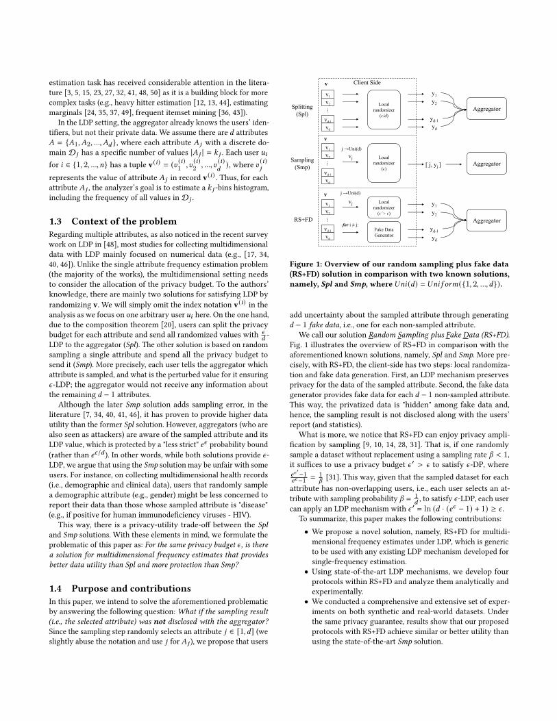
Figure 1: Overview of our random sampling plus fake data(RS+FD) solution in comparison with two known solutions,namely, Spl and Smp, where𝑈𝑛𝑖 (𝑑) = 𝑈𝑛𝑖 𝑓 𝑜𝑟𝑚({1, 2, ..., 𝑑}).
add uncertainty about the sampled attribute through generating
𝑑 − 1 fake data, i.e., one for each non-sampled attribute.
We call our solution Random Sampling plus Fake Data (RS+FD).Fig. 1 illustrates the overview of RS+FD in comparison with the
aforementioned known solutions, namely, Spl and Smp. More pre-
cisely, with RS+FD, the client-side has two steps: local randomiza-
tion and fake data generation. First, an LDP mechanism preserves
privacy for the data of the sampled attribute. Second, the fake data
generator provides fake data for each 𝑑 − 1 non-sampled attribute.
This way, the privatized data is "hidden" among fake data and,
hence, the sampling result is not disclosed along with the users’
report (and statistics).
What is more, we notice that RS+FD can enjoy privacy ampli-
fication by sampling [9, 10, 14, 28, 31]. That is, if one randomly
sample a dataset without replacement using a sampling rate 𝛽 < 1,it suffices to use a privacy budget 𝜖 ′ > 𝜖 to satisfy 𝜖-DP, where
𝑒𝜖′−1
𝑒𝜖−1 = 1𝛽[31]. This way, given that the sampled dataset for each
attribute has non-overlapping users, i.e., each user selects an at-
tribute with sampling probability 𝛽 = 1𝑑, to satisfy 𝜖-LDP, each user
can apply an LDP mechanism with 𝜖 ′ = ln (𝑑 · (𝑒𝜖 − 1) + 1) ≥ 𝜖 .
To summarize, this paper makes the following contributions:
• We propose a novel solution, namely, RS+FD for multidi-
mensional frequency estimates under LDP, which is generic
to be used with any existing LDP mechanism developed for
single-frequency estimation.
• Using state-of-the-art LDP mechanisms, we develop four
protocols within RS+FD and analyze them analytically and
experimentally.
• We conducted a comprehensive and extensive set of exper-
iments on both synthetic and real-world datasets. Under
the same privacy guarantee, results show that our proposed
protocols with RS+FD achieve similar or better utility than
using the state-of-the-art Smp solution.
Paper’s outline: The remainder of this paper is organized as fol-
lows. In Section 2, we revise the privacy notions that we are con-
sidering, i.e., LDP, the LDP mechanisms we further analyze in this
paper, and amplification by sampling. In Section 3, we introduce
our RS+FD solution, the integration of state-of-the-art LDP mecha-
nisms within RS+FD, and their analysis. In Section 4, we present
experimental results. In Section 5, we discuss our results and re-
view related work. Lastly, in Section 6, we present the concluding
remarks and future directions.
2 PRELIMINARIESIn this section, we briefly recall LDP (Subsection 2.1), the LDP
mechanisms we will apply in this paper (Subsection 2.2), and am-
plification by sampling (Subsection 2.3).
2.1 Local differential privacyLocal differential privacy, initially formalized in [28], protects an
individual’s privacy during the data collection process. A formal
definition of LDP is given in the following:
Definition 1 (𝜖-Local Differential Privacy). A randomizedalgorithm A satisfies 𝜖-LDP if, for any pair of input values 𝑣1, 𝑣2 ∈𝐷𝑜𝑚𝑎𝑖𝑛(A) and any possible output 𝑦 of A:
Pr[A(𝑣1) = 𝑦] ≤ 𝑒𝜖 · Pr[A(𝑣2) = 𝑦].
Similar to the centralized model of DP, LDP also enjoys several
important properties, e.g., immunity to post-processing (𝐹 (A) is 𝜖-LDP for any function 𝐹 ) and composability [20]. That is, combining
the results from𝑚 differentially private mechanisms also satisfies
DP. If these mechanisms are applied separately in disjointed subsets
of the dataset, 𝜖 = 𝑚𝑎𝑥 (𝜖1-, . . . , 𝜖𝑚)-LDP (parallel composition).
On the other hand, if these mechanisms are sequentially applied to
the same dataset, 𝜖 =∑𝑚𝑖=1 𝜖𝑖 -LDP (sequential composition).
2.2 LDP mechanismsRandomized response (RR), a surveying technique proposed by
Warner [47], has been the building block for many LDPmechanisms.
Let 𝐴 𝑗 = {𝑣1, 𝑣2, ..., 𝑣𝑘 𝑗} be a set of 𝑘 𝑗 = |𝐴 𝑗 | values of a given
attribute and let 𝜖 be the privacy budget, we review two state-
of-the-art LDP mechanisms for single-frequency estimation (a.k.a.
frequency oracles) that will be used in this paper.
2.2.1 Generalized randomized response (GRR). The k-Ary RR [27]
mechanism extends RR to the case of 𝑘 𝑗 ≥ 2 and is also referred
to as direct encoding [41] or generalized RR (GRR) [43, 45, 49].
Throughout this paper, we use the term GRR for this LDP mech-
anism. Given a value 𝐵 = 𝑣𝑖 , GRR(𝑣𝑖 ) outputs the true value 𝑣𝑖
with probability 𝑝 = 𝑒𝜖
𝑒𝜖+𝑘 𝑗−1 , and any other value 𝑣𝑙 for 𝑙 ≠ 𝑖 with
probability 𝑞 =1−𝑝𝑘 𝑗−1 = 1
𝑒𝜖+𝑘 𝑗−1 . GRR satisfies 𝜖-LDP since𝑝𝑞 = 𝑒𝜖 .
The estimated frequency 𝑓 (𝑣𝑖 ) that a value 𝑣𝑖 occurs, for 𝑖 ∈[1, 𝑘 𝑗 ], is calculated as [41, 43]:
𝑓 (𝑣𝑖 ) =𝑁𝑖 − 𝑛𝑞𝑛(𝑝 − 𝑞) , (1)
in which 𝑁𝑖 is the number of times the value 𝑣𝑖 has been reported
and 𝑛 is the total number of users. In [41], it is shown that this is an
unbiased estimation of the true frequency, and the variance of this
estimation is 𝑉𝑎𝑟 [𝑓 (𝑣𝑖 )] = 𝑞 (1−𝑞)𝑛 (𝑝−𝑞)2 +
𝑓 (𝑣𝑖 ) (1−𝑝−𝑞)𝑛 (𝑝−𝑞) . In the case of
small 𝑓 (𝑣𝑖 ) ∼ 0, this variance is dominated by the first term. Thus,
the approximate variance of this estimation for GRR is [41]:
𝑉𝑎𝑟 [𝑓𝐺𝑅𝑅 (𝑣𝑖 )] =𝑒𝜖 + 𝑘 𝑗 − 2𝑛(𝑒𝜖 − 1)2
. (2)
2.2.2 Optimized unary encoding (OUE). For a given value 𝑣 , 𝐵 =
𝐸𝑛𝑐𝑜𝑑𝑒 (𝑣), where 𝐵 = [0, 0, ..., 1, 0, ...0], a 𝑘 𝑗 -bit array in which
only the 𝑣-th position is set to one. Subsequently, the bits from 𝐵
are flipped, depending on two parameters 𝑝 and 𝑞, to generate a
privatized vector 𝐵′. More precisely, 𝑃𝑟 [𝐵′[𝑖] = 1] = p if 𝐵 [𝑖] = 1and 𝑃𝑟 [𝐵′[𝑖] = 1] = q if 𝐵 [𝑖] = 0. This unary-encoding (UE)
mechanism satisfies 𝜖-LDP for 𝜖 = 𝑙𝑛
(𝑝 (1−𝑞)(1−𝑝)𝑞
)[23].Wang et al. [41]
propose optimized UE (OUE), which selects "optimized" parameters
(𝑝 = 12 and 𝑞 = 1
𝑒𝜖+1 ) to minimize the approximate variance ofUE-based mechanisms while still satisfying 𝜖-LDP. The estimation
method used in (1) equally applies to OUE. As shown in [41], the
OUE approximate variance is calculated as:
𝑉𝑎𝑟 [𝑓𝑂𝑈𝐸 (𝑣𝑖 )] =4𝑒𝜖
𝑛(𝑒𝜖 − 1)2. (3)
2.2.3 Adaptive LDP mechanism. Comparing (2) with (3), elements
𝑘 𝑗 − 2 + 𝑒𝜖 is replaced by 4𝑒𝜖 . Thus, as highlighted in [41], when
𝑘 𝑗 < 3𝑒𝜖 + 2, the utility loss with GRR is lower than the one of
OUE. Throughout this paper, we will use the term adaptive (ADP)
to denote this best-effort and dynamic selection of LDP mechanism.
2.3 Privacy amplification by samplingOne well-known approach for increasing the privacy of a DP mech-
anism is to apply the mechanism to a random subsample of the
dataset [9, 10, 14, 28, 31]. The intuition is that an attacker is unable
to distinguish which data samples were used in the analysis. Li et
al. [31, Theorem 1] theoretically prove this effect.
Theorem 1. Amplification by Sampling [31]. Let A be an 𝜖 ′-DP mechanism and S to be a sampling algorithm with sampling rate𝛽 . Then, if S is first applied to a dataset D, which is later privatized
with A, the derived result satisfies DP with 𝜖 = ln(1 + 𝛽 (𝑒𝜖′ + 1)
).
3 RANDOM SAMPLING PLUS FAKE DATAIn this section, we present the overview of our RS+FD solution (Sub-
section 3.1), and the integration of the local randomizers presented
in Subsection 2.2 within RS+FD (Subsections 3.2, 3.3, and 3.4).
3.1 Overview of RS+FDWe consider the local DP model, in which there are two entities,
namely, users and the aggregator (an untrusted curator). Let 𝑛
be the total number of users, 𝑑 be the total number of attributes,
k = [𝑘1, 𝑘2, ..., 𝑘𝑑 ] be the domain size of each attribute, A be a
local randomizer, and 𝜖 be the privacy budget. Each user holds a
tuple v = (𝑣1, 𝑣2, ..., 𝑣𝑑 ), i.e., a private value per attribute.Client-Side. The client-side is split into two steps, namely, local
randomization and fake data generation (cf. Fig. 1). Initially, each
user samples a unique attribute 𝑗 uniformly at random and applies
an LDP mechanism to its value 𝑣 𝑗 . Indeed, RS+FD is generic to
be applied with any existing LDP mechanisms (e.g., GRR [27], UE-
based protocols [23, 41], Hadamard Response [3]). Next, for each𝑑−1 non-sampled attribute 𝑖 , the user generates one random fake data.
Finally, each user sends the (LDP or fake) value of each attribute
to the aggregator, i.e., a tuple y = (𝑦1, 𝑦2, ..., 𝑦𝑑 ). This way, thesampling result is not disclosed with the aggregator. In summary,
Alg. 1 exhibits the pseudocode of our RS+FD solution.
Aggregator. For each attribute 𝑗 ∈ [1, 𝑑], the aggregator performs
frequency (or histogram) estimation on the collected data by re-
moving bias introduced by the local randomizer and fake data.
Algorithm 1 Random Sampling plus Fake Data (RS+FD)
Input : tuple v = (𝑣1, 𝑣2, ..., 𝑣𝑑 ) , domain size of attributes k = [𝑘1, 𝑘2, ..., 𝑘𝑑 ], privacyparameter 𝜖 , local randomizer A.
Output : privatized tuple y = (𝑦1, 𝑦2, ..., 𝑦𝑑 ) .1: 𝜖′ = ln (𝑑 · (𝑒𝜖 − 1) + 1) ⊲ amplification by sampling [31]
2: 𝑗 ← 𝑈𝑛𝑖 𝑓 𝑜𝑟𝑚 ( {1, 2, ..., 𝑑 }) ⊲ Selection of attribute to privatize
3: 𝐵 𝑗 ← 𝑣𝑗4: 𝑦 𝑗 ← A(𝐵 𝑗 , 𝑘 𝑗 , 𝜖
′) ⊲ privatize data of the sampled attribute
5: for 𝑖 ∈ {1, 2, ..., 𝑑 }/𝑗 do ⊲ non-sampled attributes
6: 𝑦𝑖 ← Uniform( {1, ..., 𝑘𝑖 }) ⊲ generate fake data7: end for
return : y = (𝑦1, 𝑦2, ..., 𝑦𝑑 ) ⊲ sampling result is not disclosed
Privacy analysis. Let A be any existing LDP mechanism, Algo-
rithm 1 satisfies 𝜖-LDP, in a way that 𝜖 ′ = ln (𝑑 · (𝑒𝜖 − 1) + 1).Indeed, we observe that our scenario is equivalent to sampling a
dataset D without replacement with sampling rate 𝛽 = 1𝑑in the
centralized setting of DP, which enjoys privacy amplification (cf.
Subsection 2.3). With the local model, users privatize their data
locally with a DP model. This way, to satisfy 𝜖-LDP, an amplified
privacy parameter 𝜖 ′ > 𝜖 can be used.
Limitations. Similar to other sampling-based methods for collect-
ing multidimensional data under LDP [17, 34, 40, 46], our RS+FD
solution also entails sampling error, which is due to observing a
sample instead of the entire population. In addition, in comparison
with the Smp solution, RS+FD requires more computation on the
user side because of the fake data generation part. Yet, communica-
tion cost is still equal to the Spl solution, i.e., each user sends one
message per attribute. Lastly, while RS+FD utilizes an amplified
𝜖 ′ ≥ 𝜖 , there is also bias generated from uniform fake data that
may require a sufficient number of users 𝑛 to eliminate the noise.
3.2 RS+FD with GRRClient side. Integrating GRR as the local randomizerA into Alg. 1
(RS+FD[GRR]) requires no modification. Initially, on the client-
side, each user randomly samples an attribute 𝑗 . Next, the value
𝑣 𝑗 is privatized with GRR (cf. Subsection 2.2.1) using the size of
the domain 𝑘 𝑗 and the privacy parameter 𝜖 ′. In addition, for each
non-sampled 𝑑 − 1 attribute 𝑖 , the user also generates fake data
uniformly at random according to the domain size 𝑘𝑖 . Lastly, the
user transmits the privatize tuple y, which includes the LDP value
of the true data "hidden" among fake data.
Aggregator RS+FD[GRR]. On the server-side, for each attribute
𝑗 ∈ [1, 𝑑], the aggregator estimates 𝑓 (𝑣𝑖 ) for the frequency of each
value 𝑖 ∈ [1, 𝑘 𝑗 ] as:
𝑓 (𝑣𝑖 ) =𝑁𝑖𝑑𝑘 𝑗 − 𝑛(𝑑 − 1 + 𝑞𝑘 𝑗 )
𝑛𝑘 𝑗 (𝑝 − 𝑞), (4)
in which 𝑁𝑖 is the number of times the value 𝑣𝑖 has been reported,
𝑝 = 𝑒𝜖′
𝑒𝜖′+𝑘 𝑗−1
, and 𝑞 =1−𝑝𝑘 𝑗−1 .
Theorem 2. For 𝑗 ∈ [1, 𝑑], the estimation result 𝑓 (𝑣𝑖 ) in (4) is anunbiased estimation of 𝑓 (𝑣𝑖 ) for any value 𝑣𝑖 ∈ D𝑗 .
Proof 2
𝐸 [𝑓 (𝑣𝑖 )] = 𝐸
[𝑁𝑖𝑑𝑘 𝑗 − 𝑛(𝑑 − 1 + 𝑞𝑘 𝑗 )
𝑛𝑘 𝑗 (𝑝 − 𝑞)
]=
𝑑
𝑛(𝑝 − 𝑞) 𝐸 [𝑁𝑖] −𝑑 − 1 + 𝑞𝑘 𝑗𝑘 𝑗 (𝑝 − 𝑞)
.
Let us focus on
𝐸 [𝑁𝑖 ] =1
𝑑(𝑝𝑛𝑓 (𝑣𝑖 ) + 𝑞(𝑛 − 𝑛𝑓 (𝑣𝑖 ))) +
𝑑 − 1𝑑𝑘 𝑗
𝑛
=𝑛
𝑑
(𝑓 (𝑣𝑖 ) (𝑝 − 𝑞) + 𝑞 +
𝑑 − 1𝑘 𝑗
).
Thus,
𝐸 [𝑓 (𝑣𝑖 )] = 𝑓 (𝑣𝑖 ).
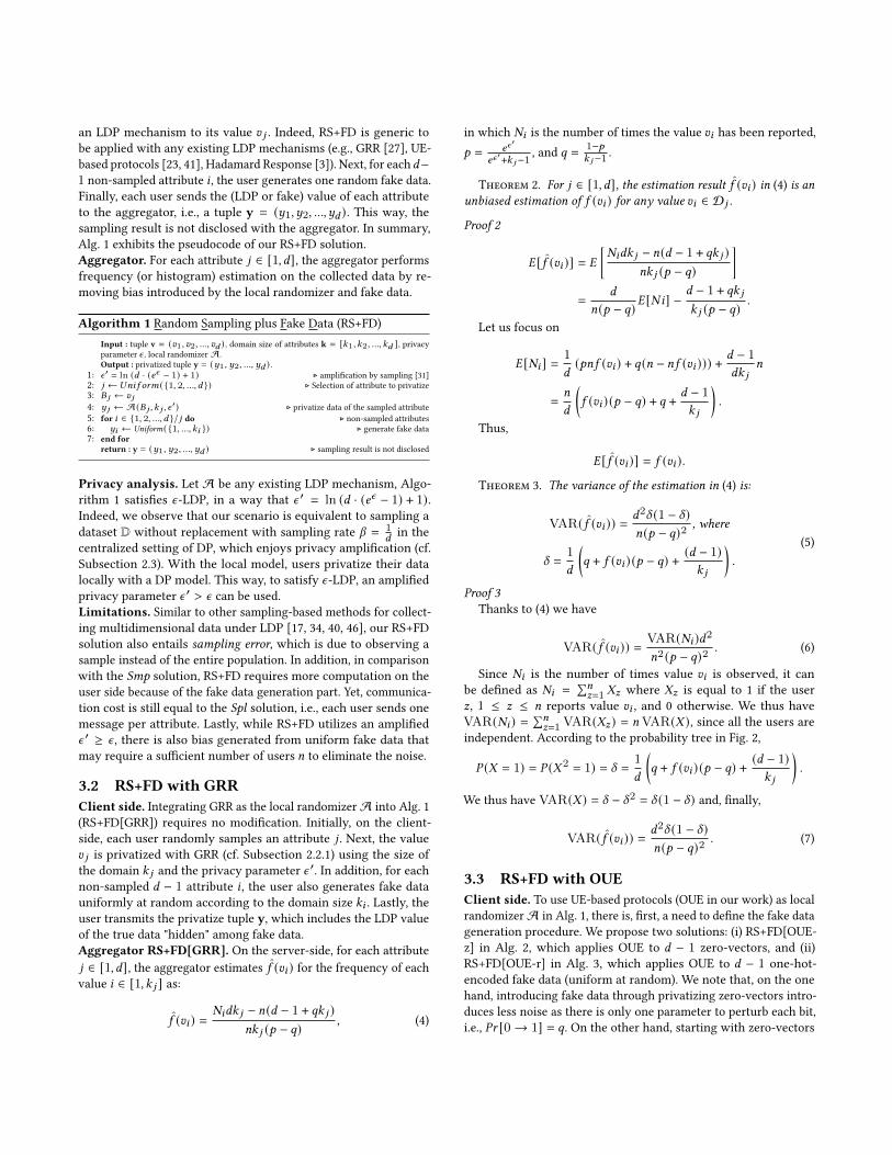
Theorem 3. The variance of the estimation in (4) is:
VAR(𝑓 (𝑣𝑖 )) =𝑑2𝛿 (1 − 𝛿)𝑛(𝑝 − 𝑞)2
, where
𝛿 =1
𝑑
(𝑞 + 𝑓 (𝑣𝑖 ) (𝑝 − 𝑞) +
(𝑑 − 1)𝑘 𝑗
).
(5)
Proof 3Thanks to (4) we have
VAR(𝑓 (𝑣𝑖 )) =VAR(𝑁𝑖 )𝑑2
𝑛2 (𝑝 − 𝑞)2. (6)
Since 𝑁𝑖 is the number of times value 𝑣𝑖 is observed, it can
be defined as 𝑁𝑖 =∑𝑛𝑧=1 𝑋𝑧 where 𝑋𝑧 is equal to 1 if the user
𝑧, 1 ≤ 𝑧 ≤ 𝑛 reports value 𝑣𝑖 , and 0 otherwise. We thus have
VAR(𝑁𝑖 ) =∑𝑛𝑧=1VAR(𝑋𝑧) = 𝑛VAR(𝑋 ), since all the users are
independent. According to the probability tree in Fig. 2,
𝑃 (𝑋 = 1) = 𝑃 (𝑋2 = 1) = 𝛿 =1
𝑑
(𝑞 + 𝑓 (𝑣𝑖 ) (𝑝 − 𝑞) +
(𝑑 − 1)𝑘 𝑗
).
We thus have VAR(𝑋 ) = 𝛿 − 𝛿2 = 𝛿 (1 − 𝛿) and, finally,
VAR(𝑓 (𝑣𝑖 )) =𝑑2𝛿 (1 − 𝛿)𝑛(𝑝 − 𝑞)2
. (7)
3.3 RS+FD with OUEClient side. To use UE-based protocols (OUE in our work) as local
randomizerA in Alg. 1, there is, first, a need to define the fake data
generation procedure. We propose two solutions: (i) RS+FD[OUE-
z] in Alg. 2, which applies OUE to 𝑑 − 1 zero-vectors, and (ii)
RS+FD[OUE-r] in Alg. 3, which applies OUE to 𝑑 − 1 one-hot-
encoded fake data (uniform at random). We note that, on the one
hand, introducing fake data through privatizing zero-vectors intro-
duces less noise as there is only one parameter to perturb each bit,
i.e., 𝑃𝑟 [0→ 1] = 𝑞. On the other hand, starting with zero-vectors
RS+FD
Fake data
𝐵′ = 𝑣𝑙≠𝑖1 − 1/𝑘𝑗
𝐵′ = 𝑣𝑖1/𝑘 𝑗1 − 1/𝑑
True data
𝐵 = 𝑣𝑙≠𝑖
𝐵′ = 𝑣𝑖𝑞
𝐵′ = 𝑣𝑖
𝑝
𝐵 = 𝑣𝑖
𝐵′ = 𝑣𝑙≠𝑖𝑞
𝐵′ = 𝑣𝑖𝑝
1/𝑑
Figure 2: Probability tree for Eq. (4) (RS+FD[GRR]).
Algorithm 2 RS+FD[OUE-z]
Input : tuple v = (𝑣1, 𝑣2, ..., 𝑣𝑑 ) , domain size of attributes k = [𝑘1, 𝑘2, ..., 𝑘𝑑 ], privacyparameter 𝜖 , local randomizer OUE.
Output : privatized tuple B′ = (𝐵′1, 𝐵′2, ..., 𝐵
′𝑑) .
1: 𝜖′ = ln (𝑑 · (𝑒𝜖 − 1) + 1) ⊲ amplification by sampling [31]
2: 𝑗 ← 𝑈𝑛𝑖 𝑓 𝑜𝑟𝑚 ( {1, 2, ..., 𝑑 }) ⊲ Selection of attribute to privatize
3: 𝐵 𝑗 = 𝐸𝑛𝑐𝑜𝑑𝑒 (𝑣𝑗 ) = [0, 0, ..., 1, 0, ...0] ⊲ one-hot-encoding
4: 𝐵′𝑗← 𝑂𝑈𝐸 (𝐵 𝑗 , 𝜖
′) ⊲ privatize real data with OUE
5: for 𝑖 ∈ {1, 2, ..., 𝑑 }/𝑗 do ⊲ non-sampled attributes
6: 𝐵𝑖 ← [0, 0, ..., 0] ⊲ initialize zero-vectors
7: 𝐵′𝑖← 𝑂𝑈𝐸 (𝐵𝑖 , 𝜖′) ⊲ randomize zero-vector with OUE
8: end forreturn : B′ = (𝐵′1, 𝐵
′2, ..., 𝐵
′𝑑) ⊲ sampling result is not disclosed
Algorithm 3 RS+FD[OUE-r]
Input : tuple v = (𝑣1, 𝑣2, ..., 𝑣𝑑 ) , domain size of attributes k = [𝑘1, 𝑘2, ..., 𝑘𝑑 ], privacyparameter 𝜖 , local randomizer OUE.
Output : privatized tuple B′ = (𝐵′1, 𝐵′2, ..., 𝐵
′𝑑) .
1: 𝜖′ = ln (𝑑 · (𝑒𝜖 − 1) + 1) ⊲ amplification by sampling [31]
2: 𝑗 ← 𝑈𝑛𝑖 𝑓 𝑜𝑟𝑚 ( {1, 2, ..., 𝑑 }) ⊲ Selection of attribute to privatize
3: 𝐵 𝑗 = 𝐸𝑛𝑐𝑜𝑑𝑒 (𝑣𝑗 ) = [0, 0, ..., 1, 0, ...0] ⊲ one-hot-encoding
4: 𝐵′𝑗← 𝑂𝑈𝐸 (𝐵 𝑗 , 𝜖
′) ⊲ privatize real data with OUE
5: for 𝑖 ∈ {1, 2, ..., 𝑑 }/𝑗 do ⊲ non-sampled attributes
6: 𝑦𝑖 ← Uniform( {1, ..., 𝑘𝑖 }) ⊲ generate fake data7: 𝐵𝑖 ← 𝐸𝑛𝑐𝑜𝑑𝑒 (𝑦𝑖 ) ⊲ one-hot-encoding
8: 𝐵′𝑖← 𝑂𝑈𝐸 (𝐵𝑖 , 𝜖′) ⊲ randomize fake data with OUE
9: end forreturn : B′ = (𝐵′1, 𝐵
′2, ..., 𝐵
′𝑑) ⊲ sampling result is not disclosed
may not suffice to "hide" the sampled attribute if the perturbation
probability 𝑞 is too small. Studying this effect is out of the scope of
this paper and is left as future work.
Aggregator RS+FD[OUE-z]. On the server-side, if fake data are
generated with OUE applied to zero-vectors, as in Alg. 2, for each
attribute 𝑗 ∈ [1, 𝑑], the aggregator estimates 𝑓 (𝑣𝑖 ) for the frequencyof each value 𝑖 ∈ [1, 𝑘 𝑗 ] as:
𝑓 (𝑣𝑖 ) =𝑑 (𝑁𝑖 − 𝑛𝑞)𝑛(𝑝 − 𝑞) , (8)
in which 𝑁𝑖 is the number of times the value 𝑣𝑖 has been reported,
𝑛 is the total number of users, 𝑝 = 12 , and 𝑞 = 1
𝑒𝜖′+1 .
Theorem 4. For 𝑗 ∈ [1, 𝑑], the estimation result 𝑓 (𝑣𝑖 ) in (8) is anunbiased estimation of 𝑓 (𝑣𝑖 ) for any value 𝑣𝑖 ∈ D𝑗 .
Proof 4
𝐸 [𝑓 (𝑣𝑖 )] = 𝐸
[𝑑 (𝑁𝑖 − 𝑛𝑞)𝑛(𝑝 − 𝑞)
]=𝑑 (𝐸 [𝑁𝑖 ] − 𝑛𝑞)
𝑛(𝑝 − 𝑞)
=𝑑
𝑛(𝑝 − 𝑞) 𝐸 [𝑁𝑖 ] −𝑑𝑞
𝑝 − 𝑞 .
We have successively
𝐸 [𝑁𝑖 ] =𝑛
𝑑(𝑝 𝑓 (𝑣𝑖 ) + 𝑞(1 − 𝑓 (𝑣𝑖 ))) +
(𝑑 − 1)𝑛𝑞𝑑
=𝑛
𝑑(𝑓 (𝑣𝑖 ) (𝑝 − 𝑞) + 𝑑𝑞) .
Thus,
𝐸 [𝑓 (𝑣𝑖 )] = 𝑓 (𝑣𝑖 ).
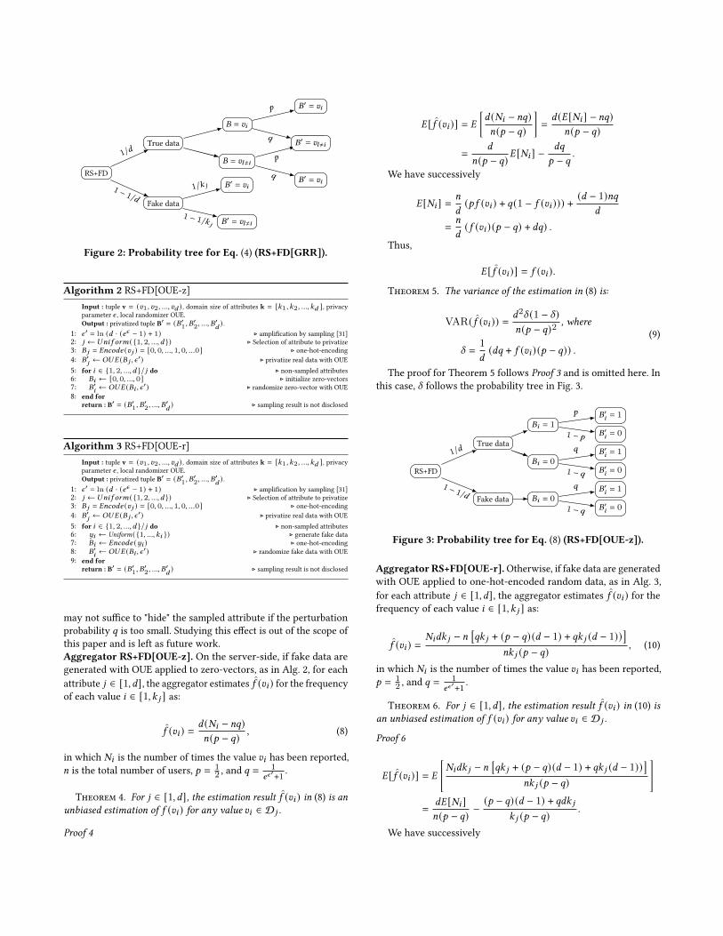
Theorem 5. The variance of the estimation in (8) is:
VAR(𝑓 (𝑣𝑖 )) =𝑑2𝛿 (1 − 𝛿)𝑛(𝑝 − 𝑞)2
, where
𝛿 =1
𝑑(𝑑𝑞 + 𝑓 (𝑣𝑖 ) (𝑝 − 𝑞)) .
(9)
The proof for Theorem 5 follows Proof 3 and is omitted here. In
this case, 𝛿 follows the probability tree in Fig. 3.
RS+FD
Fake data 𝐵𝑖 = 0𝐵′𝑖 = 01 − 𝑞
𝐵′𝑖 = 1𝑞1 − 1/𝑑
True data
𝐵𝑖 = 0𝐵′𝑖 = 01 − 𝑞
𝐵′𝑖 = 1𝑞
𝐵𝑖 = 1𝐵′𝑖 = 01 − 𝑝
𝐵′𝑖 = 1𝑝
1/𝑑
Figure 3: Probability tree for Eq. (8) (RS+FD[OUE-z]).
Aggregator RS+FD[OUE-r].Otherwise, if fake data are generatedwith OUE applied to one-hot-encoded random data, as in Alg. 3,
for each attribute 𝑗 ∈ [1, 𝑑], the aggregator estimates 𝑓 (𝑣𝑖 ) for thefrequency of each value 𝑖 ∈ [1, 𝑘 𝑗 ] as:
𝑓 (𝑣𝑖 ) =𝑁𝑖𝑑𝑘 𝑗 − 𝑛
[𝑞𝑘 𝑗 + (𝑝 − 𝑞) (𝑑 − 1) + 𝑞𝑘 𝑗 (𝑑 − 1))
]𝑛𝑘 𝑗 (𝑝 − 𝑞)
, (10)
in which 𝑁𝑖 is the number of times the value 𝑣𝑖 has been reported,
𝑝 = 12 , and 𝑞 = 1
𝑒𝜖′+1 .
Theorem 6. For 𝑗 ∈ [1, 𝑑], the estimation result 𝑓 (𝑣𝑖 ) in (10) isan unbiased estimation of 𝑓 (𝑣𝑖 ) for any value 𝑣𝑖 ∈ D𝑗 .
Proof 6
𝐸 [𝑓 (𝑣𝑖 )] = 𝐸
[𝑁𝑖𝑑𝑘 𝑗 − 𝑛
[𝑞𝑘 𝑗 + (𝑝 − 𝑞) (𝑑 − 1) + 𝑞𝑘 𝑗 (𝑑 − 1))
]𝑛𝑘 𝑗 (𝑝 − 𝑞)
]=
𝑑𝐸 [𝑁𝑖 ]𝑛(𝑝 − 𝑞) −
(𝑝 − 𝑞) (𝑑 − 1) + 𝑞𝑑𝑘 𝑗𝑘 𝑗 (𝑝 − 𝑞)
.
We have successively
𝐸 [𝑁𝑖 ] =𝑛
𝑑(𝑝𝑓 (𝑣𝑖 ) + 𝑞(1 − 𝑓 (𝑣𝑖 ))) +
𝑛(𝑑 − 1)𝑑
( 𝑝𝑘 𝑗+𝑘 𝑗 − 1𝑘 𝑗
𝑞)
=𝑛
𝑑(𝑓 (𝑣𝑖 ) (𝑝 − 𝑞) + 𝑞)) +
𝑛(𝑑 − 1)𝑑𝑘 𝑗
(𝑝 − 𝑞 + 𝑘 𝑗𝑞).
Thus,
𝐸 [𝑓 (𝑣𝑖 )] = 𝑓 (𝑣𝑖 ).
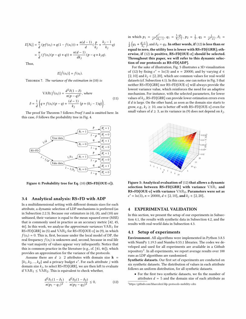
Theorem 7. The variance of the estimation in (10) is:
VAR(𝑓 (𝑣𝑖 )) =𝑑2𝛿 (1 − 𝛿)𝑛(𝑝 − 𝑞)2
, where
𝛿 =1
𝑑
(𝑞 + 𝑓 (𝑣𝑖 ) (𝑝 − 𝑞) +
(𝑑 − 1)𝑘 𝑗
(𝑝 + (𝑘 𝑗 − 1)𝑞
) ).
(11)
The proof for Theorem 7 follows Proof 3 and is omitted here. In
this case, 𝛿 follows the probability tree in Fig. 4.
RS+FD
Fake data
𝐵𝑖 = 0𝐵′𝑖 = 01 − 𝑞
𝐵′𝑖 = 1𝑞1 − 1/𝑘𝑗
𝐵𝑖 = 1𝐵′𝑖 = 01 − 𝑝
𝐵′𝑖 = 1𝑝
1/𝑘 𝑗1 − 1/𝑑
True data
𝐵𝑖 = 0𝐵′𝑖 = 01 − 𝑞
𝐵′𝑖 = 1𝑞
𝐵𝑖 = 1𝐵′𝑖 = 01 − 𝑝
𝐵′𝑖 = 1𝑝
1/𝑑
Figure 4: Probability tree for Eq. (10) (RS+FD[OUE-r]).
3.4 Analytical analysis: RS+FD with ADPIn a multidimensional setting with different domain sizes for each
attribute, a dynamic selection of LDP mechanisms is preferred (as
in Subsection 2.2.3). Because our estimators in (4), (8), and (10) are
unbiased, their variance is equal to the mean squared error (MSE)
that is commonly used in practice as an accuracy metric [42, 45,
46]. In this work, we analyze the approximate variances VAR1 for
RS+FD[GRR] in (5) and VAR2 for RS+FD[OUE-z] in (9), in which
𝑓 (𝑣𝑖 ) = 0. This is, first, because under the local model of DP, the
real frequency 𝑓 (𝑣𝑖 ) is unknown and, second, because in real life
the vast majority of values appear very infrequently. Notice that
this is common practice in the literature (e.g., cf. [41, 46]), which
provides an approximation for the variance of the protocols.
Assume there are 𝑑 ≥ 2 attributes with domain size k =
[𝑘1, 𝑘2, ..., 𝑘𝑑 ] and a privacy budget 𝜖 ′. For each attribute 𝑗 with
domain size 𝑘 𝑗 , to select RS+FD[GRR], we are then left to evaluate
if VAR1 ≤ VAR2. This is equivalent to check whether,
𝑑2𝛿1 (1 − 𝛿1)𝑛(𝑝1 − 𝑞1)2
− 𝑑2𝛿2 (1 − 𝛿2)𝑛(𝑝2 − 𝑞2)2
≤ 0, (12)
in which 𝑝1 = 𝑒𝜖′
𝑒𝜖′+𝑘 𝑗−1
, 𝑞1 =1−𝑝1
𝑘 𝑗−1 , 𝑝2 = 12 , 𝑞2 = 1
𝑒𝜖′+1 , 𝛿1 =
1𝑑
(𝑞1 + 𝑑−1
𝑘 𝑗
), and 𝛿2 = 𝑞2. In other words, if (12) is less than or
equal to zero, the utility loss is lowerwith RS+FD[GRR]; oth-erwise, if (12) is positive, RS+FD[OUE-z] should be selected.Throughout this paper, we will refer to this dynamic selec-tion of our protocols as RS+FD[ADP].
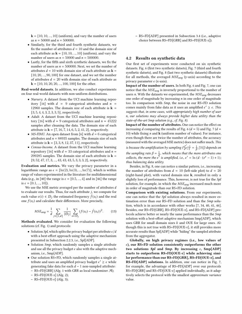
For the sake of illustration, Fig. 5 illustrates a 3D visualization
of (12) by fixing 𝜖 ′ = ln(3) and 𝑛 = 20000, and by varying 𝑑 ∈[2, 10] and 𝑘 𝑗 ∈ [2, 20], which are common values for real-world
datasets (cf. Subsection 4.1). In this case, one can notice in Fig. 5 that
neither RS+FD[GRR] nor RS+FD[OUE-z] will always provide the
lowest variance value, which reinforces the need for an adaptive
mechanism. For instance, with the selected parameters, for lower
values of 𝑘 𝑗 , RS+FD[GRR] can provide lower estimation errors even
if 𝑑 is large. On the other hand, as soon as the domain size starts to
grow, e.g., 𝑘 𝑗 ≥ 10, one is better off with RS+FD[OUE-z] even for
small values of 𝑑 ≥ 3, as its variance in (9) does not depend on 𝑘 𝑗 .
d
23
45
67
89
10
k j
5
10
15
20
VAR
1−VAR
2
−0.02
−0.01
0.00
0.01
0.02
Figure 5: Analytical evaluation of (12) that allows a dynamicselection between RS+FD[GRR] with variance VAR1 andRS+FD[OUE-z] with variance VAR2. Parameters were set as𝜖 ′ = ln(3), 𝑛 = 20000, 𝑑 ∈ [2, 10], and 𝑘 𝑗 ∈ [2, 20].
4 EXPERIMENTAL VALIDATIONIn this section, we present the setup of our experiments in Subsec-
tion 4.1, the results with synthetic data in Subsection 4.2, and the
results with real-world data in Subsection 4.3.
4.1 Setup of experimentsEnvironment. All algorithms were implemented in Python 3.8.5
with NumPy 1.19.5 and Numba 0.53.1 libraries. The codes we de-
veloped and used for all experiments are available in a Github
repository1. In all experiments, we report average results over 100
runs as LDP algorithms are randomized.
Synthetic datasets. Our first set of experiments are conducted on
six synthetic datasets. The distribution of values in each attribute
follows an uniform distribution, for all synthetic datasets.
• For the first two synthetic datasets, we fix the number of
attributes 𝑑 = 5 and the domain size of each attribute as
1https://github.com/hharcolezi/ldp-protocols-mobility-cdrs
k = [10, 10, ..., 10] (uniform), and vary the number of users
as 𝑛 = 50000 and 𝑛 = 500000.• Similarly, for the third and fourth synthetic datasets, we
fix the number of attributes 𝑑 = 10 and the domain size of
each attribute as k = [10, 10, ..., 10] (uniform), and vary the
number of users as 𝑛 = 50000 and 𝑛 = 500000.• Lastly, for the fifth and sixth synthetic datasets, we fix the
number of users as 𝑛 = 500000. Next, we set the number of
attributes 𝑑 = 10 with domain size of each attribute as k =
[10, 20, ..., 90, 100] for one dataset, and we set the number
of attributes 𝑑 = 20 with domain size of each attribute as
k = [10, 10, 20, 20, ..., 100, 100] for the other.Real-world datasets. In addition, we also conduct experiments
on four real-world datasets with non-uniform distributions.
• Nursery. A dataset from the UCI machine learning repos-
itory [16] with 𝑑 = 9 categorical attributes and 𝑛 =
12960 samples. The domain size of each attribute is k =
[3, 5, 4, 4, 3, 2, 3, 3, 5], respectively.• Adult. A dataset from the UCI machine learning reposi-
tory [16] with 𝑑 = 9 categorical attributes and 𝑛 = 45222samples after cleaning the data. The domain size of each
attribute is k = [7, 16, 7, 14, 6, 5, 2, 41, 2], respectively.• MS-FIMU. An open dataset from [6] with 𝑑 = 6 categorical
attributes and 𝑛 = 88935 samples. The domain size of each
attribute is k = [3, 3, 8, 12, 37, 11], respectively.• Census-Income. A dataset from the UCI machine learning
repository [16] with 𝑑 = 33 categorical attributes and 𝑛 =
299285 samples. The domain size of each attribute is k =
[9, 52, 47, 17, 3, ..., 43, 43, 43, 5, 3, 3, 3, 2], respectively.Evaluation and metrics. We vary the privacy parameter in a
logarithmic range as 𝜖 = [ln(2), ln(3), ..., ln(7)], which is within
range of values experimented in the literature for multidimensional
data (e.g., in [40] the range is 𝜖 = [0.5, ..., 4] and in [46] the range
is 𝜖 = [0.1, ..., 10]).We use the MSE metric averaged per the number of attributes 𝑑
to evaluate our results. Thus, for each attribute 𝑗 , we compute for
each value 𝑣 (𝑖) ∈ D𝑗 the estimated frequency 𝑓 (𝑣𝑖 ) and the real
one 𝑓 (𝑣𝑖 ) and calculate their differences. More precisely,
𝑀𝑆𝐸𝑎𝑣𝑔 =1
𝑑
∑︁𝑗 ∈[1,𝑑 ]
1
|D𝑗 |∑︁𝑣∈D𝑗
(𝑓 (𝑣𝑖 ) − 𝑓 (𝑣𝑖 ))2. (13)
Methods evaluated. We consider for evaluation the following
solutions (cf. Fig. 1) and protocols:
• Solution Spl, which splits the privacy budget per attribute 𝜖/𝑑with a best-effort approach using the adaptive mechanism
presented in Subsection 2.2.3, i.e., Spl[ADP].
• Solution Smp, which randomly samples a single attribute
and use all the privacy budget 𝜖 also with the adaptive mech-
anism, i.e., Smp[ADP].
• Our solution RS+FD, which randomly samples a single at-
tribute and uses an amplified privacy budget 𝜖 ′ ≥ 𝜖 while
generating fake data for each 𝑑 − 1 non-sampled attribute:
– RS+FD[GRR] (Alg. 1 with GRR as local randomizer A);
– RS+FD[OUE-z] (Alg. 2);
– RS+FD[OUE-r] (Alg. 3);
– RS+FD[ADP] presented in Subsection 3.4 (i.e., adaptive
choice between RS+FD[GRR] and RS+FD[OUE-z]).
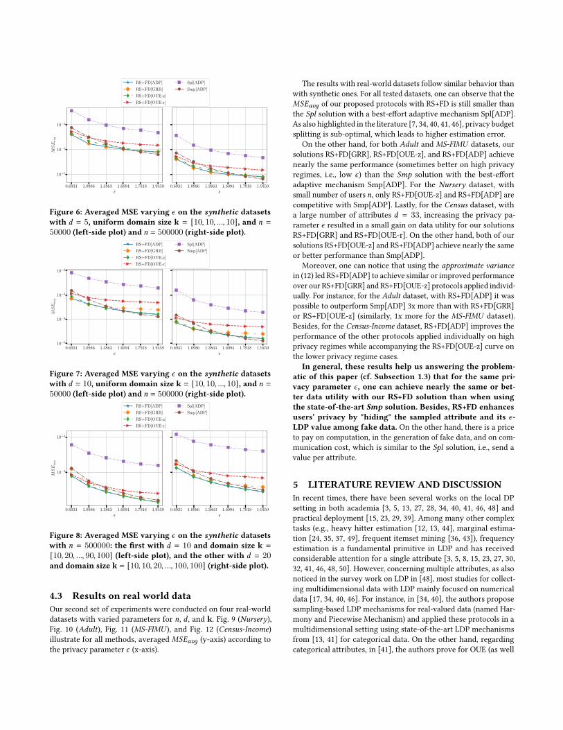
4.2 Results on synthetic dataOur first set of experiments were conducted on six synthetic
datasets. Fig. 6 (first two synthetic datsets), Fig. 7 (third and fourth
synthetic datsets), and Fig. 8 (last two synthetic datasets) illustrate
for all methods, the averaged 𝑀𝑆𝐸𝑎𝑣𝑔 (y-axis) according to the
privacy parameter 𝜖 (x-axis).
Impact of the number of users. In both Fig. 6 and Fig. 7, one can
notice that the𝑀𝑆𝐸𝑎𝑣𝑔 is inversely proportional to the number of
users 𝑛. With the datasets we experimented, the𝑀𝑆𝐸𝑎𝑣𝑔 decreases
one order of magnitude by increasing 𝑛 in one order of magnitude
too. In comparison with Smp, the noise in our RS+FD solution
comes mainly from fake data as it uses an amplified 𝜖 ′ ≥ 𝜖 . Thissuggests that, in some cases, with appropriately high number of user𝑛, our solutions may always provide higher data utility than thestate-of-the-art Smp solution (e.g., cf. Fig. 8).Impact of the number of attributes.One can notice the effect onincreasing 𝑑 comparing the results of Fig. 6 (𝑑 = 5) and Fig. 7 (𝑑 =
10) while fixing 𝑛 and k (uniform number of values). For instance,
even though there are twice the number of attributes, the accuracy
(measuredwith the averagedMSEmetric) does not suffermuch. This
is because the amplification by sampling (𝑒𝜖′−1𝑒𝜖−1 = 1
𝛽[31]) depends on
the sampling rate 𝛽 = 1𝑑, which means that the more attributes one
collects, the more the 𝜖 ′ is amplified, i.e., 𝜖 ′ = ln (𝑑 · (𝑒𝜖 − 1) + 1);thus balancing data utility.
Besides, in Fig. 8, one can notice a similar pattern, i.e., increasing
the number of attributes from 𝑑 = 10 (left-side plot) to 𝑑 = 20(right-hand plot), with varied domain size k, resulted in only a
slightly loss of performance. This, however, is not true for the Splsolution, for example, in which the𝑀𝑆𝐸𝑎𝑣𝑔 increased much more
in order of magnitude than our RS+FD solution.
Comparison with existing solutions. From our experiments,
one can notice that the Spl solution always resulted in more es-
timation error than our RS+FD solution and than the Smp solu-
tion, which is in accordance with other works [7, 34, 40, 41, 46].
Besides, our RS+FD[GRR], RS+FD[OUE-z], and RS+FD[ADP] pro-
tocols achieve better or nearly the same performance than the Smpsolution with a best-effort adaptive mechanism Smp[ADP], which
uses GRR for small domain sizes 𝑘 and OUE for large ones. Al-
though this is not true with RS+FD[OUE-r], it still provides more
accurate results than Spl[ADP] while "hiding" the sampled attribute
from the aggregator.
Globally, on high privacy regimes (i.e., low values of𝜖), our RS+FD solution consistently outperforms the othertwo solutions Spl and Smp. By increasing 𝜖, Smp[ADP]starts to outperform RS+FD[OUE-r] while achieving simi-lar performance than our RS+FD[GRR], RS+FD[OUE-z], andRS+FD[ADP] solutions. In addition, one can notice in Fig. 7,
for example, the advantage of RS+FD[ADP] over our protocols
RS+FD[GRR] and RS+FD[OUE-z] applied individually, as it adap-
tively selects the protocol with the smallest approximate variancevalue.
0.6931 1.0986 1.3863 1.6094 1.7918 1.9459
ε
10−5
10−4
10−3
MSEavg
0.6931 1.0986 1.3863 1.6094 1.7918 1.9459
ε
RS+FD[ADP]
RS+FD[GRR]
RS+FD[OUE-z]
RS+FD[OUE-r]
Spl[ADP]
Smp[ADP]
Figure 6: Averaged MSE varying 𝜖 on the synthetic datasetswith 𝑑 = 5, uniform domain size k = [10, 10, ..., 10], and 𝑛 =
50000 (left-side plot) and 𝑛 = 500000 (right-side plot).
0.6931 1.0986 1.3863 1.6094 1.7918 1.9459
ε
10−5
10−4
10−3
10−2
MSEavg
0.6931 1.0986 1.3863 1.6094 1.7918 1.9459
ε
RS+FD[ADP]
RS+FD[GRR]
RS+FD[OUE-z]
RS+FD[OUE-r]
Spl[ADP]
Smp[ADP]
Figure 7: Averaged MSE varying 𝜖 on the synthetic datasetswith 𝑑 = 10, uniform domain size k = [10, 10, ..., 10], and 𝑛 =
50000 (left-side plot) and 𝑛 = 500000 (right-side plot).
0.6931 1.0986 1.3863 1.6094 1.7918 1.9459
ε
10−4
10−3
MSEavg
0.6931 1.0986 1.3863 1.6094 1.7918 1.9459
ε
RS+FD[ADP]
RS+FD[GRR]
RS+FD[OUE-z]
RS+FD[OUE-r]
Spl[ADP]
Smp[ADP]
Figure 8: Averaged MSE varying 𝜖 on the synthetic datasetswith 𝑛 = 500000: the first with 𝑑 = 10 and domain size k =
[10, 20, ..., 90, 100] (left-side plot), and the other with 𝑑 = 20and domain size k = [10, 10, 20, ..., 100, 100] (right-side plot).
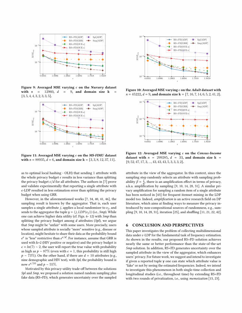
4.3 Results on real world dataOur second set of experiments were conducted on four real-world
datasets with varied parameters for 𝑛, 𝑑 , and k. Fig. 9 (Nursery),Fig. 10 (Adult), Fig. 11 (MS-FIMU ), and Fig. 12 (Census-Income)illustrate for all methods, averaged 𝑀𝑆𝐸𝑎𝑣𝑔 (y-axis) according to
the privacy parameter 𝜖 (x-axis).
The results with real-world datasets follow similar behavior than
with synthetic ones. For all tested datasets, one can observe that the
𝑀𝑆𝐸𝑎𝑣𝑔 of our proposed protocols with RS+FD is still smaller than
the Spl solution with a best-effort adaptive mechanism Spl[ADP].
As also highlighted in the literature [7, 34, 40, 41, 46], privacy budget
splitting is sub-optimal, which leads to higher estimation error.
On the other hand, for both Adult and MS-FIMU datasets, our
solutions RS+FD[GRR], RS+FD[OUE-z], and RS+FD[ADP] achieve
nearly the same performance (sometimes better on high privacy
regimes, i.e., low 𝜖) than the Smp solution with the best-effort
adaptive mechanism Smp[ADP]. For the Nursery dataset, with
small number of users 𝑛, only RS+FD[OUE-z] and RS+FD[ADP] are
competitive with Smp[ADP]. Lastly, for the Census dataset, witha large number of attributes 𝑑 = 33, increasing the privacy pa-
rameter 𝜖 resulted in a small gain on data utility for our solutions
RS+FD[GRR] and RS+FD[OUE-r]. On the other hand, both of our
solutions RS+FD[OUE-z] and RS+FD[ADP] achieve nearly the same
or better performance than Smp[ADP].
Moreover, one can notice that using the approximate variancein (12) led RS+FD[ADP] to achieve similar or improved performance
over our RS+FD[GRR] and RS+FD[OUE-z] protocols applied individ-
ually. For instance, for the Adult dataset, with RS+FD[ADP] it was
possible to outperform Smp[ADP] 3x more than with RS+FD[GRR]
or RS+FD[OUE-z] (similarly, 1x more for the MS-FIMU dataset).
Besides, for the Census-Income dataset, RS+FD[ADP] improves the
performance of the other protocols applied individually on high
privacy regimes while accompanying the RS+FD[OUE-z] curve on
the lower privacy regime cases.
In general, these results help us answering the problem-atic of this paper (cf. Subsection 1.3) that for the same pri-vacy parameter 𝜖, one can achieve nearly the same or bet-ter data utility with our RS+FD solution than when usingthe state-of-the-art Smp solution. Besides, RS+FD enhancesusers’ privacy by "hiding" the sampled attribute and its 𝜖-LDP value among fake data. On the other hand, there is a price
to pay on computation, in the generation of fake data, and on com-
munication cost, which is similar to the Spl solution, i.e., send a
value per attribute.
5 LITERATURE REVIEW AND DISCUSSIONIn recent times, there have been several works on the local DP
setting in both academia [3, 5, 13, 27, 28, 34, 40, 41, 46, 48] and
practical deployment [15, 23, 29, 39]. Among many other complex
tasks (e.g., heavy hitter estimation [12, 13, 44], marginal estima-
tion [24, 35, 37, 49], frequent itemset mining [36, 43]), frequency
estimation is a fundamental primitive in LDP and has received
considerable attention for a single attribute [3, 5, 8, 15, 23, 27, 30,
32, 41, 46, 48, 50]. However, concerning multiple attributes, as also
noticed in the survey work on LDP in [48], most studies for collect-
ing multidimensional data with LDP mainly focused on numerical
data [17, 34, 40, 46]. For instance, in [34, 40], the authors propose
sampling-based LDP mechanisms for real-valued data (named Har-
mony and Piecewise Mechanism) and applied these protocols in a
multidimensional setting using state-of-the-art LDP mechanisms
from [13, 41] for categorical data. On the other hand, regarding
categorical attributes, in [41], the authors prove for OUE (as well
0.6931 1.0986 1.3863 1.6094 1.7918 1.9459ε
10−3
10−2
MSEavg
RS+FD[ADP]
RS+FD[GRR]
RS+FD[OUE-z]
RS+FD[OUE-r]
Spl[ADP]
Smp[ADP]
Figure 9: Averaged MSE varying 𝜖 on the Nursery datasetwith 𝑛 = 12960, 𝑑 = 9, and domain size k =
[3, 5, 4, 4, 3, 2, 3, 3, 5].
0.6931 1.0986 1.3863 1.6094 1.7918 1.9459ε
10−4
10−3
10−2
MSEavg
RS+FD[ADP]
RS+FD[GRR]
RS+FD[OUE-z]
RS+FD[OUE-r]
Spl[ADP]
Smp[ADP]
Figure 10: AveragedMSE varying 𝜖 on theAdult dataset with𝑛 = 45222, 𝑑 = 9, and domain size k = [7, 16, 7, 14, 6, 5, 2, 41, 2].
0.6931 1.0986 1.3863 1.6094 1.7918 1.9459ε
10−4
10−3
MSEavg
RS+FD[ADP]
RS+FD[GRR]
RS+FD[OUE-z]
RS+FD[OUE-r]
Spl[ADP]
Smp[ADP]
Figure 11: Averaged MSE varying 𝜖 on the MS-FIMU datasetwith 𝑛 = 88935, 𝑑 = 6, and domain size k = [3, 3, 8, 12, 37, 11].
0.6931 1.0986 1.3863 1.6094 1.7918 1.9459ε
10−4
10−3
10−2
MSEavg
RS+FD[ADP]
RS+FD[GRR]
RS+FD[OUE-z]
RS+FD[OUE-r]
Spl[ADP]
Smp[ADP]
Figure 12: Averaged MSE varying 𝜖 on the Census-Incomedataset with 𝑛 = 299285, 𝑑 = 33, and domain size k =
[9, 52, 47, 17, 3, ..., 43, 43, 43, 5, 3, 3, 3, 2].
as to optimal local hashing - OLH) that sending 1 attribute with
the whole privacy budget 𝜖 results in less variance than splitting
the privacy budget 𝜖/𝑑 for all attributes. The authors in [7] prove
and validate experimentally that reporting a single attribute with
𝜖-LDP resulted in less estimation error than splitting the privacy
budget when using GRR.
However, in the aforementioned works [7, 34, 40, 41, 46], the
sampling result is known by the aggregator. That is, each user
samples a single attribute 𝑗 , applies a local randomizer to 𝑣 𝑗 , and
sends to the aggregator the tuple𝑦 = ⟨ 𝑗, 𝐿𝐷𝑃 (𝑣 𝑗 )⟩ (i.e., Smp). While
one can achieve higher data utility (cf. Figs. 6- 12) with Smp than
splitting the privacy budget among 𝑑 attributes (Spl), we argue
that Smp might be "unfair" with some users. More precisely, users
whose sampled attribute is socially "more" sensitive (e.g., disease or
location), might hesitate to share their data as the probability bound
𝑒𝜖 is "less" restrictive than 𝑒𝜖/𝑑 . For instance, assume that GRR is
used with k=2 (HIV positive or negative) and the privacy budget is
𝜖 = 𝑙𝑛(7) ∼ 2, the user will report the true value with probability
as high as 𝑝 ∼ 87% (even with 𝜖 = 1, this probability is still high
𝑝 ∼ 73%). On the other hand, if there are 𝑑 = 10 attributes (e.g.,
nine demographic and HIV test), with Spl, the probability bound is
now 𝑒𝜖/10 and 𝑝 ∼ 55%.
Motivated by this privacy-utility trade-off between the solutions
Spl and Smp, we proposed a solution named random sampling plus
fake data (RS+FD), which generates uncertainty over the sampled
attribute in the view of the aggregator. In this context, since the
sampling step randomly selects an attribute with sampling prob-
ability 𝛽 = 1𝑑, there is an amplification effect in terms of privacy,
a.k.a. amplification by sampling [9, 10, 14, 28, 31]. A similar pri-
vacy amplification for sampling a random item of a single attribute
has been noticed in [43] for frequent itemset mining in the LDP
model too. Indeed, amplification is an active research field on DP
literature, which aims at finding ways to measure the privacy in-
troduced by non-compositional sources of randomness, e.g., sam-
pling [9, 10, 14, 28, 31], iteration [25], and shuffling [11, 21, 22, 42].
6 CONCLUSION AND PERSPECTIVESThis paper investigates the problem of collecting multidimensional
data under 𝜖-LDP for the fundamental task of frequency estimation.
As shown in the results, our proposed RS+FD solution achieves
nearly the same or better performance than the state-of-the-art
Smp solution. In addition, RS+FD generates uncertainty over the
sampled attribute in the view of the aggregator, which enhances
users’ privacy. For future work, we suggest and intend to investigate
if given a reported tuple y one can state which attribute value is
"fake" or not by seeing the estimated frequencies. Indeed, we intend
to investigate this phenomenon in both single-time collection and
longitudinal studies (i.e., throughout time) by extending RS+FD
with two rounds of privatization, i.e., using memoization [15, 23].
ACKNOWLEDGMENTSThis work was supported by the Region of Bourgogne Franche-
Comté CADRAN Project and by the EIPHI-BFC Graduate School
(contract “ANR-17-EURE-0002"). All computations have been per-
formed on the "Mésocentre de Calcul de Franche-Comté".
REFERENCES[1] Martin Abadi, Andy Chu, Ian Goodfellow, H. Brendan McMahan, Ilya Mironov,
Kunal Talwar, and Li Zhang. 2016. Deep Learning with Differential Privacy
(CCS ’16). Association for Computing Machinery, New York, NY, USA, 308–318.
https://doi.org/10.1145/2976749.2978318
[2] John M. Abowd. 2018. The U.S. Census Bureau Adopts Differential Privacy.
In Proceedings of the 24th ACM SIGKDD International Conference on KnowledgeDiscovery & Data Mining. ACM. https://doi.org/10.1145/3219819.3226070
[3] Jayadev Acharya, Ziteng Sun, and Huanyu Zhang. 2019. Hadamard Response:
Estimating Distributions Privately, Efficiently, and with Little Communication.
In Proceedings of the Twenty-Second International Conference on Artificial Intelli-gence and Statistics (Proceedings of Machine Learning Research, Vol. 89), Kamalika
Chaudhuri and Masashi Sugiyama (Eds.). PMLR, 1120–1129.
[4] Ahmet Aktay et al. 2020. Google COVID-19 community mobility reports:
Anonymization process description (version 1.0). arXiv preprint arXiv:2004.04145(2020).
[5] Mario Alvim, Konstantinos Chatzikokolakis, Catuscia Palamidessi, and Anna
Pazii. 2018. Invited Paper: Local Differential Privacy on Metric Spaces: Optimiz-
ing the Trade-Off with Utility. In 2018 IEEE 31st Computer Security FoundationsSymposium (CSF). IEEE. https://doi.org/10.1109/csf.2018.00026
[6] Héber H. Arcolezi, Jean-François Couchot, Oumaya Baala, Jean-Michel Contet,
Bechara Al Bouna, and Xiaokui Xiao. 2020. Mobility modeling through mo-
bile data: generating an optimized and open dataset respecting privacy. In 2020International Wireless Communications and Mobile Computing (IWCMC). IEEE.https://doi.org/10.1109/iwcmc48107.2020.9148138
[7] Héber H. Arcolezi, Jean-François Couchot, Bechara Al Bouna, and Xiaokui Xiao.
2021. Longitudinal Collection and Analysis of Mobile Phone Data with Local
Differential Privacy. In IFIP Advances in Information and Communication Tech-nology. Springer International Publishing, 40–57. https://doi.org/10.1007/978-3-
030-72465-8_3
[8] Héber H. Arcolezi, Jean-François Couchot, Selene Cerna, Christophe Guyeux,
Guillaume Royer, Béchara Al Bouna, and Xiaokui Xiao. 2020. Forecasting the
number of firefighter interventions per region with local-differential-privacy-
based data. Computers & Security 96 (Sept. 2020), 101888. https://doi.org/10.
1016/j.cose.2020.101888
[9] Borja Balle, Gilles Barthe, and Marco Gaboardi. 2018. Privacy amplification
by subsampling: tight analyses via couplings and divergences. In Proceedingsof the 32nd International Conference on Neural Information Processing Systems.6280–6290.
[10] Borja Balle, Gilles Barthe, and Marco Gaboardi. 2020. Privacy profiles and ampli-
fication by subsampling. Journal of Privacy and Confidentiality 10, 1 (2020).
[11] Borja Balle, James Bell, Adrià Gascón, and Kobbi Nissim. 2019. The Privacy
Blanket of the Shuffle Model. In Advances in Cryptology – CRYPTO 2019. SpringerInternational Publishing, 638–667. https://doi.org/10.1007/978-3-030-26951-7_22
[12] Raef Bassily, Kobbi Nissim, Uri Stemmer, and Abhradeep Thakurta. 2017. Practical
locally private heavy hitters. arXiv preprint arXiv:1707.04982 (2017).[13] Raef Bassily and Adam Smith. 2015. Local, Private, Efficient Protocols for Succinct
Histograms. In Proceedings of the forty-seventh annual ACM symposium on Theoryof Computing. ACM. https://doi.org/10.1145/2746539.2746632
[14] Kamalika Chaudhuri and Nina Mishra. 2006. When Random Sampling Preserves
Privacy. In Lecture Notes in Computer Science. Springer Berlin Heidelberg, 198–213.https://doi.org/10.1007/11818175_12
[15] Bolin Ding, Janardhan Kulkarni, and Sergey Yekhanin. 2017. Collecting Telemetry
Data Privately. In Advances in Neural Information Processing Systems 30, I. Guyon,U. V. Luxburg, S. Bengio, H. Wallach, R. Fergus, S. Vishwanathan, and R. Garnett
(Eds.). Curran Associates, Inc., 3571–3580.
[16] Dheeru Dua and Casey Graff. 2017. UCI Machine Learning Repository. http:
//archive.ics.uci.edu/ml
[17] John C. Duchi, Michael I. Jordan, and Martin J. Wainwright. 2018. Minimax
Optimal Procedures for Locally Private Estimation. J. Amer. Statist. Assoc. 113,521 (Jan. 2018), 182–201. https://doi.org/10.1080/01621459.2017.1389735
[18] Cynthia Dwork. 2006. Differential Privacy. In Automata, Languages and Pro-gramming. Springer Berlin Heidelberg, 1–12. https://doi.org/10.1007/11787006_1
[19] Cynthia Dwork, Frank McSherry, Kobbi Nissim, and Adam Smith. 2006. Cali-
brating Noise to Sensitivity in Private Data Analysis. In Theory of Cryptography.Springer Berlin Heidelberg, 265–284. https://doi.org/10.1007/11681878_14
[20] Cynthia Dwork, Aaron Roth, et al. 2014. The algorithmic foundations of differ-
ential privacy. Foundations and Trends® in Theoretical Computer Science 9, 3–4(2014), 211–407.
[21] Úlfar Erlingsson, Vitaly Feldman, Ilya Mironov, Ananth Raghunathan, Shuang
Song, Kunal Talwar, and Abhradeep Thakurta. 2020. Encode, shuffle, ana-
lyze privacy revisited: Formalizations and empirical evaluation. arXiv preprintarXiv:2001.03618 (2020).
[22] Úlfar Erlingsson, Vitaly Feldman, Ilya Mironov, Ananth Raghunathan, Kunal
Talwar, and Abhradeep Thakurta. 2019. Amplification by Shuffling: From Local
to Central Differential Privacy via Anonymity. In Proceedings of the ThirtiethAnnual ACM-SIAM Symposium on Discrete Algorithms. Society for Industrial and
Applied Mathematics, 2468–2479. https://doi.org/10.1137/1.9781611975482.151
[23] Úlfar Erlingsson, Vasyl Pihur, and Aleksandra Korolova. 2014. RAPPOR: Ran-
domized Aggregatable Privacy-Preserving Ordinal Response. In Proceedingsof the 2014 ACM SIGSAC Conference on Computer and Communications Secu-rity (Scottsdale, Arizona, USA). ACM, New York, NY, USA, 1054–1067. https:
//doi.org/10.1145/2660267.2660348
[24] Giulia Fanti, Vasyl Pihur, and Úlfar Erlingsson. 2016. Building a RAPPOR with the
Unknown: Privacy-Preserving Learning of Associations and Data Dictionaries.
Proceedings on Privacy Enhancing Technologies 2016, 3 (May 2016), 41–61. https:
//doi.org/10.1515/popets-2016-0015
[25] Vitaly Feldman, Ilya Mironov, Kunal Talwar, and Abhradeep Thakurta. 2018.
Privacy Amplification by Iteration. In 2018 IEEE 59th Annual Symposium onFoundations of Computer Science (FOCS). 521–532. https://doi.org/10.1109/FOCS.
2018.00056
[26] Simson Garfinkel. 2021. Implementing Differential Privacy for the 2020 Census.
USENIX Association.
[27] Peter Kairouz, Keith Bonawitz, and Daniel Ramage. 2016. Discrete distribution
estimation under local privacy. In International Conference on Machine Learning.PMLR, 2436–2444.
[28] Shiva Prasad Kasiviswanathan, Homin K. Lee, Kobbi Nissim, Sofya Raskhod-
nikova, and Adam Smith. 2008. What Can We Learn Privately?. In 2008 49thAnnual IEEE Symposium on Foundations of Computer Science. IEEE. https:
//doi.org/10.1109/focs.2008.27
[29] Stephan Kessler, Jens Hoff, and Johann-Christoph Freytag. 2019. SAP HANA
goes private. Proceedings of the VLDB Endowment 12, 12 (Aug. 2019), 1998–2009.https://doi.org/10.14778/3352063.3352119
[30] Jong Wook Kim, Dae-Ho Kim, and Beakcheol Jang. 2018. Application of Local
Differential Privacy to Collection of Indoor Positioning Data. IEEE Access 6 (2018),4276–4286. https://doi.org/10.1109/access.2018.2791588
[31] Ninghui Li, Wahbeh Qardaji, and Dong Su. 2012. On sampling, anonymization,
and differential privacy or, k-anonymizationmeets differential privacy. In Proceed-ings of the 7th ACM Symposium on Information, Computer and CommunicationsSecurity - ASIACCS '12. ACM Press. https://doi.org/10.1145/2414456.2414474
[32] Zitao Li, Tianhao Wang, Milan Lopuhaä-Zwakenberg, Ninghui Li, and Boris
Škoric. 2020. Estimating Numerical Distributions under Local Differential Privacy.
In Proceedings of the 2020 ACM SIGMOD International Conference on Managementof Data. ACM. https://doi.org/10.1145/3318464.3389700
[33] David McCandless, Tom Evans, Miriam Quick, Ella Hollowood, Christian Miles,
Dan Hampson, and Duncan Geere. 2021. World’s Biggest Data Breaches &
Hacks. https://www.informationisbeautiful.net/visualizations/worlds-biggest-
data-breaches-hacks/. Online; accessed 11 March 2021.
[34] Thông T. Nguyên, Xiaokui Xiao, Yin Yang, Siu Cheung Hui, Hyejin Shin, and
Junbum Shin. 2016. Collecting and Analyzing Data from Smart Device Users
with Local Differential Privacy. ArXiv abs/1606.05053 (2016).
[35] Fan Peng, Shaohua Tang, Bowen Zhao, and Yuxian Liu. 2019. A privacy-
preserving data aggregation of mobile crowdsensing based on local differential
privacy. In Proceedings of the ACM Turing Celebration Conference - China. ACM.
https://doi.org/10.1145/3321408.3321602
[36] Zhan Qin, Yin Yang, Ting Yu, Issa Khalil, Xiaokui Xiao, and Kui Ren. 2016.
Heavy Hitter Estimation over Set-Valued Data with Local Differential Privacy. In
Proceedings of the 2016 ACM SIGSAC Conference on Computer and CommunicationsSecurity. ACM. https://doi.org/10.1145/2976749.2978409
[37] Xuebin Ren, Chia-mu Yu, Weiren Yu, Shusen Yang, Senior Member, Xinyu Yang,
Julie A Mccann, Philip S Yu, and Life Fellow. 2018. LoPub : High-Dimensional
Crowdsourced Data. 13, 9 (2018), 2151–2166. https://doi.org/10.1109/TIFS.2018.
2812146
[38] Ryan Rogers, Subbu Subramaniam, Sean Peng, David Durfee, Seunghyun Lee,
Santosh Kumar Kancha, Shraddha Sahay, and Parvez Ahammad. 2020. LinkedIn’s
Audience Engagements API: A privacy preserving data analytics system at scale.
arXiv preprint arXiv:2002.05839 (2020).[39] Apple Differential Privacy Team. 2017. Learning with privacy at
scale. https://docs-assets.developer.apple.com/ml-research/papers/learning-
with-privacy-at-scale.pdf. Online; accessed 11 March 2021.
[40] Ning Wang, Xiaokui Xiao, Yin Yang, Jun Zhao, Siu Cheung Hui, Hyejin Shin,
Junbum Shin, and Ge Yu. 2019. Collecting and Analyzing Multidimensional Data
with Local Differential Privacy. In 2019 IEEE 35th International Conference onData Engineering (ICDE). IEEE. https://doi.org/10.1109/icde.2019.00063
[41] Tianhao Wang, Jeremiah Blocki, Ninghui Li, and Somesh Jha. 2017. Locally
Differentially Private Protocols for Frequency Estimation. In 26th USENIX Security
Symposium (USENIX Security 17). USENIX Association, Vancouver, BC, 729–745.
[42] Tianhao Wang, Bolin Ding, Min Xu, Zhicong Huang, Cheng Hong, Jingren Zhou,
Ninghui Li, and Somesh Jha. 2020. Improving utility and security of the shuffler-
based differential privacy. Proceedings of the VLDB Endowment 13, 13 (Sept. 2020),3545–3558. https://doi.org/10.14778/3424573.3424576
[43] Tianhao Wang, Ninghui Li, and Somesh Jha. 2018. Locally Differentially Private
Frequent Itemset Mining. In 2018 IEEE Symposium on Security and Privacy (SP).IEEE. https://doi.org/10.1109/sp.2018.00035
[44] Tianhao Wang, Ninghui Li, and Somesh Jha. 2021. Locally Differentially Private
Heavy Hitter Identification. IEEE Transactions on Dependable and Secure Com-puting 18, 2 (March 2021), 982–993. https://doi.org/10.1109/tdsc.2019.2927695
[45] Tianhao Wang, Milan Lopuhaa-Zwakenberg, Zitao Li, Boris Skoric, and Ninghui
Li. 2020. Locally Differentially Private Frequency Estimation with Consistency.
In Proceedings 2020 Network and Distributed System Security Symposium. Internet
Society. https://doi.org/10.14722/ndss.2020.24157
[46] Teng Wang, Jun Zhao, Zhi Hu, Xinyu Yang, Xuebin Ren, and Kwok-Yan Lam.
2021. Local Differential Privacy for data collection and analysis. Neurocomputing
426 (Feb. 2021), 114–133. https://doi.org/10.1016/j.neucom.2020.09.073
[47] Stanley L. Warner. 1965. Randomized Response: A Survey Technique for Elimi-
nating Evasive Answer Bias. J. Amer. Statist. Assoc. 60, 309 (March 1965), 63–69.
https://doi.org/10.1080/01621459.1965.10480775
[48] Xingxing Xiong, Shubo Liu, Dan Li, Zhaohui Cai, and Xiaoguang Niu. 2020. A
Comprehensive Survey on Local Differential Privacy. Security and CommunicationNetworks 2020 (Oct. 2020), 1–29. https://doi.org/10.1155/2020/8829523
[49] Zhikun Zhang, Tianhao Wang, Ninghui Li, Shibo He, and Jiming Chen. 2018.
CALM: Consistent adaptive local marginal for marginal release under local
differential privacy. Proceedings of the ACM Conference on Computer and Com-munications Security (2018), 212–229. https://doi.org/10.1145/3243734.3243742
[50] Dan Zhao, Hong Chen, Suyun Zhao, Xiaoying Zhang, Cuiping Li, and Ruixuan
Liu. 2019. Local Differential Privacy with K-anonymous for Frequency Estimation.
In 2019 IEEE International Conference on Big Data (Big Data). IEEE. https://doi.
org/10.1109/bigdata47090.2019.9006022