Random variate generation for unimodal and monotone …luc.devroye.org/devroye-unimodal+monotone.pdf · Random Variate Generation for Unimodal and Monotone Densities ... can be obtained

Computing 32, 43-68 (1984) Computing �9 by Springer-Verlag 1984

Random Variate Generation for Unimodal and Monotone Densities

L. Devroye, Montreal

Received December 3, 1981 ; revised May 10, 1982

Abstract - - Zusammenfassung

Random Variate Generation for Unimodal and Monotone Densities. We consider the problem of generating random variates with a monotone nonincreasing density on [0, ~). No bounds are known that would allow a straightforward application of the rejection method, and the inverse of the distribution function is not explicitly known either. We develop the inversion/rejection method, and show how it can be used for all monotone densities, even those with an infinite peak at 0 and unbounded support, provided only that the densityfand the distribution function F can be computed for each x. A theoretical analysis of the average time behaviour of the algorithms is included.

AMS Subject Classifications: 65C 10, 65C05.

Key words and phrases: Random variate generation, rejection method, inversion method, unimodality, Khintchine's theorem, average time analysis, Newton-Raphson method, table methods.

Erzeugung yon ZufaUsvariabein mit monotonen oder unimodalen Dichtefunktionen. Wir betrachten das Problem der Erzeugung von Zufallsvariablen mit monoton nichtsteigender Dichtefunktion im Intervall [0, ~). Schranken, die eine direkte Anwendung der Zurfickweisungsmethode erlauben wiirden sowie die Umkehrfunktion der Verteilung sind nicht bekannt. Wir entwickeln die Umkchr/Zuriickweisungsme- thode und zeigen ihre Anwendbarkeit auf alle monotonen Dichten, sogar auf solche, die eine Polstelle bei 0 besitzen und die einen unbeschrfinkten Wertebereich haben. Vorausgesetzt ist lediglich, daB f u n d F an jeder Stelle berechenbar sind. Eine theoretische Analyse des mittleren Zeitverhaltens der Atgorithmen ist beigefiigt.

1. Introduction

In this paper we give algorithms that can be used for the computer generation of random variables with a unimodal densi tyfwhen no bounds are available fo r f tha t would allow us to use the rejection method in a straightforward manner. We assume that a perfect uniform [0, 1] random variate generator is given, capable of generating an i. i.d. (independent identically distributed) sequence U1, U2 . . . . of uniform [0, 1] random variates. The techniques considered here are

(i) generah they can be applied to all unimodal densities with given mode, regardless of the size of the tail or the height of the peak; the densities are not assumed to belong to a parametric family, nor are bounds needed for them;

44 L. Devroye:

(ii) exact: if all the operations can be carried out with infinite precision, then the generated random variates have density f ; no approximations are allowed;

(iii) efficient: the average t ime needed per random variable should be reasonable. Of course, general algorithms of the type given here cannot be expected to be faster than algorithms designed for specific families of densities.

We will try, wherever possible, to give the statistical properties of the algorithms such as the average number of iterations per random variate, and so forth. For example, if T is the time taken by an algorithm, then we are looking for simple expressions and simple upper bounds for E (7), the average time per random variate. These should depend upon general constants only, such as the supremum off , the support off , or parameters used in the design of the algorithm. General algorithms with well-understood properties will survive longer than ad hoc algorithms that are known to perform well on specific examples but whose general properties are not clear. Our results about E (7) are based upon the not so unrealistic assumption that the common operations + , - , *, /, mod, truncate, compare, move, generate a uniform random variate, log, and exp take a given constant time.

The reader is assumed to have a basic knowledge of the common principles in non- uniform random variate generation, such as the principles of inversion, rejection, squeezing, composition, and aliasing (see Schmeiser (1980) for a survey with bibliography). The present paper is a short version of a survey and study reported in Devroye (1982).

2. The Inversion/Rejection Method

There are situations in which the rejection method can be applied with minimal knowledge about f, e.g. it can be applied whenever we know that f i s bounded by c, and the support o f f is contained in [0, 11. But if we are not given the constant c in this example, it is not clear how one should proceed without a drastic modification of the rejection method.

If F is the distribution function off, then F-1 (U) has density f w h e n U is uniformly distributed on [0, 11. Unfortunately, we are usually not given F - 1 explicitly, so that the inversion method must be implemented through the numerical solution of the equation F (X) -- U for X. This would, strictly speaking, take an infinite amount of time. The main contribution of this paper is the development of the inversion/rejection method applicable when both f and F are given (but not F - 1), and when f is known to belong to a broad class of densities (such as all unimodal densities).

The principle is simple: partition R into a countable number of intervals A1, A2, ... (this is a fixed partition), and let Pi be the probability under f of A i (this is computable since F is given). Then, proceed as follows:

Step 1: [Inversion. 1 Generate a uniform [-0, 11 random variate U, set I n 1, S ~ p l . While U > S do: I +-- I + l, S ~- S + pr [I now satisfies P (I = i) = pi, all i. It could have been generated by a method other than sequential search, but that would require the storage of the p~'s.l

Random Variate Generation for Unimodat and Monotone Densities 45

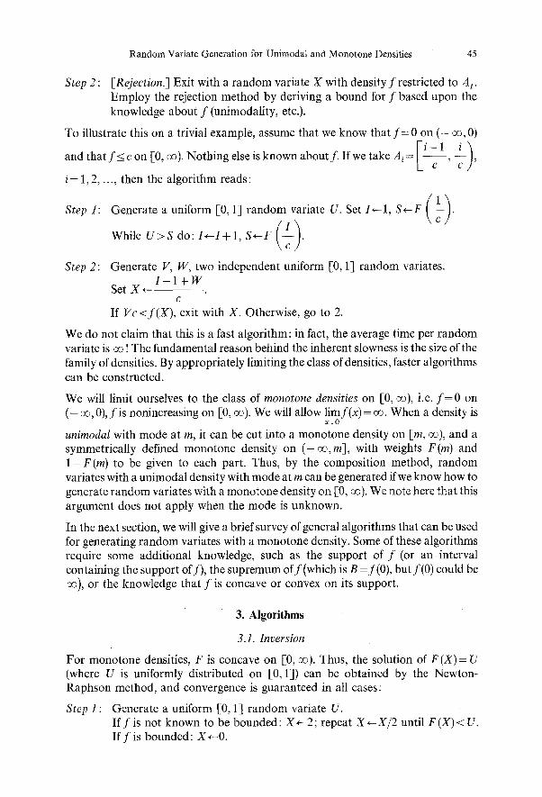
Step 2 : [Rejection.] Exit with a random variate X with density f restricted to A I. Employ the rejection method by deriving a bound for f based upon the knowledge about f (unimodality, etc.).

To illustrate this on a trivial example, assume that we know that f = 0 on ( - oo, 0)

and that f_< c on [0, oo). Nothing e!se is known about f . If we take A~ = , , c

i = 1,2,.. . , then the algorithm reads:

Stepl: Generate a uniform [0,1] random variate U. S e t I ~ I , S + - F ( I ~ .

W ile

\ c /

Step 2: Generate V, W, two independent uniform [0, 1] random variates. I - I + W

Set X * c

If Vc <f(X) , exit with X. Otherwise, go to 2.

We do not claim that this is a fast algorithm: in fact, the average time per random variate is oo ! The fundamental reason behind the inherent slowness is the size of the family of densities. By appropriately limiting the class of densities, faster algorithms can be constructed.

We will limit ourselves to the class of monotone densities on [0, oo), i.e. f = 0 on ( -o% 0), f is nonincreasing on [0, ~) . We will allow l imf(x)= oo. When a density is

x.L0

unimodal with mode at m, it can be cut into a monotone density on [m, oo), and a symmetrically defined monotone density on ( - o % m], with weights F(m) and 1-F(m) to be given to each part. Thus, by the composition method, random variates with a unimodal density with mode at m can be generated if we know how to generate random variates with a monotone density on [0, oo). We note here that this argument does not apply when the mode is unknown.

In the next section, we will give a brief survey of general algorithms that can be used for generating random variates with a monotone density. Some of these algorithms require some additional knowledge, such as the support of f (or an interval containing the support off) , the supremum off(which is B =f(0) , but f(0) could be oo), or the knowledge that f is concave or convex on its support.

3. Algorithms

3.1. Inversion

For monotone densities, F is concave on [0, ~) . Thus, the solution of F (X)= U (where U is uniformly distributed on [0, 1]) can be obtained by the Newton- Raphson method, and convergence is guaranteed in all cases:

Step I : Generate a uniform [0, 1] random variate U. If f is not known to be bounded: X ~ 2 ; repeat X ~ X / 2 until F ( X ) < U. I f f is bounded: X+-0.

46 L. Devroye:

Step 2: X*--X-(F(X)-U)/f(X). Go to 2.

This procedure does not halt. In practice, on a finite wordsize computer, one keeps on iterating until the value of X remains unchanged. Thus, the average times obtained in a timing experiment will depend very heavily on the wordsize of the computer, and the distribution function F.

When F is not given, the inversion method is hard to implement. The most valid attempt at obtaining a general algorithm for generating a random variate when only f i s given, is that of Ahrens and Kohrt (1981) (see also Kohrt (1980)), based upon the method of guide tables (Chen and Asau (1973)): strictly speaking however, the inversion algorithm given above stopped after a finite number of iterations, and the general method of Ahrens and Kohrt are not exact in the sense (ii) described in the introduction.

3.2. Rejection

In this section we assume only that f is monotone, and that

(i) f ( x ) = 0 outside [0, 1];

(ii) f(x)<_ B for all x, where B is known.

If B is not known, it can be computed as f (0), and if the support of f is not known, or exceeds [0, 13, then with a scaling adjustment the support can be made exactly equal to [0, 1] or it can be made equal to [0, c] where c is guaranteed not to exceed 1. The ordinary rejection method for generating a random variate X with density f , proceeds as follows:

Step 1: Generate two independent uniform [0, 1] random variates X and V.

Step 2: If VB<_f(X), exit with X. Otherwise, go to 1.

On the average, step 1 is executed B times. In families of densities with shape parameters, B often depends upon the shape parameter, and can grow very large for some values of the shape parameter. Thus, the ordinary rejection method can be intolerably slow, and we cannot give any guarantees about its speed. If it were not for the fact that this method can be improved upon dramatically without much effort, we would not have mentioned it in this paper.

Because the area under f is 1, we must have

I f(x)<_ ,x>0,

x

for all monotone densities f . If f is also known to be convex, this bound can be sharpened to f(x)< 1/(2 x): find the point x where f ' ( x ) = - 1. The area of the triangle formed by the axes and the tangent to f at x is at most 1 (because f is convex); but the area is exactly 2xf(x). To treat both cases simultaneously, we

1 assume that xf(x) <_-~ where k = 2, 1 according to whether f i s known to be convex or not.

Random Variate Generation for Unimodal and Monotone Densities 47

Thus, we have f(x)_<min B , ~ x , 0_<x_<l.

The area under the top curve is 1 (1 +log (kB)). It is proportional to the density

g (x)=rain (B, 1/(kx))k/(1 +log (kB)), which has distribution function

f kBx 1 +log (kB)' 0 _< x _< 1/(kB),

1 +log(xkB) 1/(kB)<_x<_ 1. 1 +log(kB) '

A random variate with density g can easily be obtained by inversion, and the modified rejection algorithm is:

Step ! : Generate two independent uniform I-0, 11 random variates U and V.

Step 2: If U < 1/(1 + log (kB)), set X +- U (1 + log (k B))/(kB). If VB <_f(X), exit with X. Otherwise, go to 1.

If U>l/(l+log(kB)), set X+--(kB) -1 exp(U(l+log(kB))-l). If V<_ kXf(X), exit with X. Otherwise, go to 1.

The average number of executions of step 1 is 1 (1 +log(kB)). When k = 1, this is

less than B whenever B > e. In most applications the improvement over the ordinary rejection method is noticeable if not spectacular. The computation of kB and 1 +log(kB) should be done in a set-up step. When f is convex (k=2), the average number of exectutions of step 1 is about half of what it was for k = 1. In a sense, the knowledge that f is convex contributes at least 50~ to the useful knowledge about f for random variate generation.

None of the rejection methods have times that remain bounded as B-o o% but they are very short and easy to understand; no tables or large set-up times are required either.

3.3. Inversion/Rejection by HaIvin 9

In this section we will apply the general inversion/rejection principle to the family of all monotone densities f with support contained in [0, 1]. We assume that f and F can be computed exactly in constant time. The sequential search for the inversion step proceeds by looking at the intervals It, 1), [rt, t), [r 2 t, rt), etc. where r, t~(0, 1) are constants to be determined. The term "halving" is used because of the obvious

1 popularity of the choice r = t = - - . The algorithm can be reduced to the following form: 2

Step 1 : Generate a uniform [-0, 1] random variate U. Set (X,X*)~(t, 1). While U> F(X) : (X,X*)~(rX, X). [At the end of this, we know that the solution of F (x)= U belongs to (X, X*).]

48 L. D e v r o y e :

Step 2 : Generate two independent uniform [0, 1] random variates V and W. Set Y*--X + V ( X * - X ) . [ Y is uniformly distributed on [X, X*].] If W<f( Y ) / f ( X ) , exit with Y. Otherwise, go to 2.

If f is known to be convex on [0, 11, then we could consider rejection from a trapezoidal dominating curve joining (X , f (X)) and (X*,f(X*)). The changes needed in the algorithm:

In step 1: Compute Z*--f (X) and Z**- f (X*) at end of step 1.

In step 2: Replace all of step 2 by the following: generate three independent uniform [0, 1] random variates, U, V and W.

Y ~ - X + R ( X * - X ) (Y has a density pro- Let R ~ m i n U, V Z _ Z ,

portional to the trapezoid determined on [X, X*1 by the points [Z, Z*1). Let T ~ W(Z + R (Z* - Z)). [Squeeze step. Optional.l If T<Z*, exit with Y. [Acceptance/rejection step.l If T<_f(Y), exit with Y. Otherwise, go to 2.

R e m a r k 1 :

The efficiency of the algorithm can be increased by storing a table of constants ( f (x), F (x)) for x = 1, t, rt, r 2 t, r 3 t, . . .. This will pay off when many random variates are needed from the same distribution. Because only finite tables can be stored, we would still need some version of the halving algorithm for the lower part of the interval [0, 11. Also, the statistical properties of the algorithm do not depend upon the presence of a partial table.

There are two big contributors to the average time E (7) of the inversion/rejection algorithm:

(i) E (Ns): the average number of steps in the sequential interval search; (ii) E(Nr): the average number of iterations in the rejection step;

this is equal to the total area under the dominating curve; in the case of inversion/rejection by halving, the dominating curve is a collection of rectangles with bases [t, 1], [rt, t], etc. and heights f(t), f(rt), etc.

T h e o r e m 1 : 1 1

Let HO0= ~ log - - . f ( x )dx . Then 0 X

log t H (J) . ~ t 1 + ~ + ~ <_ 1 + I f ( x ) . log - -dx / log - - < E (N~)

log - - log -- o x r ?" F

t t t 1 _ l o g t H ( f ) <_1+ ~ f + ~ f ( x ) . l o g - - d x / l o g - - < 2 + ~ - 4

0 o X Y - - 1 log- - log- -

r Y

R a n d o m Var ia te Gene ra t i on for U n i m o d a l and M o n o t o n e Densities 49

For t = r, the simple outer bounds for E (N~) just read

Also,

H ( f ) H ( J ) _<E(N~)_< 1 + - -

I I log - - log - -

r r

1 I < E ( N ~ ) _ < - - f + f ( t ) ( 1 - t ) < - - f N - - ,

r o r o r

where the last two inequalities only hold when t = r.

Proof: Note that 1 o~ t r i - 1 o~

E ( N s ) = f f + Z ( i + l ) I f = l + Z i t i=1 t r i i=1

t r i - 1

I f . t r l

t 1 For x ~ [ t r i, t r i - 1), we have 0 < i - log - - / l o g - - < 1. Thus,

X r

t 1 t O<_E(N~)- f ( x ) l o g - - l o g - ~ - d x - l < _ f f .

0 X r o

All the s ta tements involving E (Ns) follow trivially.

Next , we have

E (N~) = ~ f ( t r i) (tr I-1 - tr i) +f ( t ) (1 - t) i=1

tr~ tri-1 _ tr i <

I f " tr i_tr i+l ~ f ( t ) ( 1 - t ) i = l tr I+1

] t r

= - - I f + f ( t ) ( 1 - t) g 0

_<-- f w h e n t = r . r 0

Theorem 1 shows that regardless of the choice of t and r, the difficulty inherent in f i s appropr ia te ly measured by/-/0c). This quant i ty can of course be infinite, in which case E (Ns) = oe. Often H (f) can be computed or est imated beforehand. In theorem 2 below, we give some inequalities that link H (f) to bet ter known quantities such as the mean, sup f , and the L l o g + L no rm o f f .

Theorem 2:

(i) For all monotone densities,

1 H Or) > log f x f ( x ) dx"

(ii) For all monotone densities on [0, 1],

1 _</-/Oq_< 1 + log (f(0)). 4 Computing 32/1

50 L. Devroye :

(iii) For all monotone densities, 4

f l o g + f<_H(f)<_2 ~ f log+ f + - - . e

Thus, H (]) is finite if and only if f l o g + f is integrable, i.e. f ~ L log+ L.

Proof: (i) follows from the convexity of - log(x) and Jensen's inequality (see for example Feller, 1971). The second inequality (1 < H (f)) uses the fact that - l o g (x) and f(x) are both nonincreasing on [0, 1], and therefore, by Steffensen's inequality (1925),

1 1 1

-log(x) f (x )dx> S -log(x) dx ~ f (x )dx= 1. 0 0 0

The upper bound in (ii) is a special case of another inequality of Steffensen (1918): if 0 _<f< 1, and if g is nonincreasing and integrable on [0, 13, then

1 i 1 ~ g(x) f (x)dx< g(x)dx where a - - ~ f ( x ) d x . 0 0 0

Let g (x)= - l o g (x), and replace f(x) by f(x)/sup f. Thus, a = 1/sup f , and

~ - log(x)dx=a l+log 0

give the desired result. The upper bound in (iii) is a Young-type inequality found in Hardy, Littlewood and Polya (1952, theorem 239). (This inequality does not use the

1 monotonicity of f.) The lower bound in (iii) follows from f(x)<_--.

X

Example 1:

We consider the betw('[, a + 1:) density f(x) = (a + 1) 1 - x) a, 0 _~ x _~ 1, where a > 0 is a ,parameter. We have sup f=a+~, and ~xf(x)dx=l/(a+2). By (i) and (ii) of theor.em2, log(a+2)<_H(f)<_l+log(a+l), and thus H ( f ) ~ l o g a as a - ~ . By theorem 1, we can then conclude that if r, t are fixed, E (T) must grow as log a as a---~ ~ .

Remark 2: [Convex densities.]

When the modification for convex densities is implemented, the statistical properties of E (Nr) change somewhat, but those of E (Ns) remain the same. For example, it is

1 easy to show that the inequality E (Nr)_<-- valid for t = r can be replaced by the

r

tighter inequality E(Nr)<~

Remark 3: [Choice of r.] 1

Assume that t = r. If we keep r fixed, then E (Ns) >_ 1 + H (f)/log - - implies that the r

average time of the algorithm grows at least as a constant times H (f). Considering

R a n d o m Var i a t e G e n e r a t i o n f o r U n i m o d a l a n d M o n o t o n e Densi t ies 51

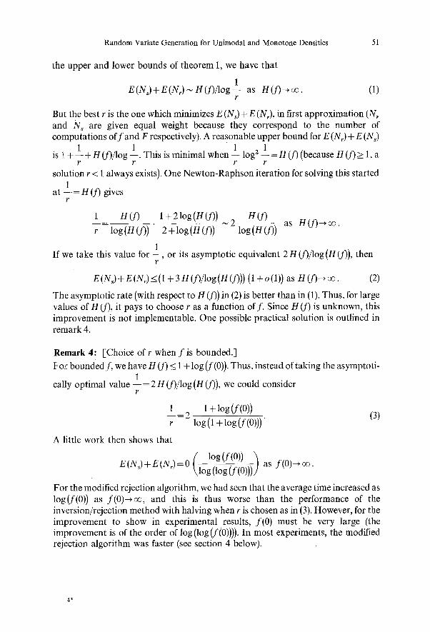
the upper and lower bounds of theorem 1, we have that

1 E(Us)+E(N,.)~H(f)/log-- as H(f)--+az. (1)

r

But the best r is the one which minimizes E (Ns) + E (Nr), in first approximation (Nr and Ns are given equal weight because they correspond to the number of computations o f f and F respectively). A reasonable upper bound for E (N,) + E (Ns)

1 1 1 is 1 + - - + H (f)/log 1 . This is minimal when - - log z - - = H (f) (because H (f) >_ 1, a

r r r r

solution r < 1 always exists). One Newton-Raphson iteration for solving this started 1

at - - = H (f) gives r

1 H(f ) 1+ 2 log (H(f)) H(f ) r = log (H (f)) 2 + log (H (f)) ~ 2 log (H (f)) as H (f) o ~ .

1 If we take this value for - - , or its asymptotic equivalent 2 H (f)/log (H (f)), then

r

E(Ns)+E(Nr)<_(l+3H(f)/log(n(f))) (1 +o(1)) as H ( f ) ~ o o . (2)

The asymptotic rate (with respect to H (f)) in (2) is better than in (1). Thus, for large values of H (f), it pays to choose r as a function of f. Since H (f) is unknown, this improvement is not implementable. One possible practical solution is outlined in remark 4.

Remark 4: [-Choice of r when f is bounded.]

For bounded f, we have H 09 _< 1 + log (f(0)). Thus, instead of taking the asymptoti- 1

cally optimal value - - = 2 H (f)/log (H (f)), we could consider r

1 1 + log (f(0)) - - = 2 (3) r log (1 + log (f(0)))"

A little work then shows that

( l o g ( f ( O ) ) "~ E (ms) + E (mr) = 0 \ log (log (f(0)))} as f ( 0 ) ~ ~ .

For the modified rejection algorithm, we had seen that the average time increased as log(f(0)) as f ( 0 ) ~ , and this is thus worse than the performance of the inversion/rejection method with halving when r is chosen as in (3). However, for the improvement to show in experimental results, f(0) must be very large (the improvement is of the order of log (log (f(0)))). In most experiments, the modified rejection algorithm was faster (see section 4 below).

4*

52 L. Devroye:

3.4. Inversion~Rejection by Doubling

Assume that f is a monotone density bounded by B, and that f and F can be computed: f can have unbounded support. We organize the interval search by looking at [0, t), It, tr), [tr, tr2),.., where t > 0 and r > 1 are constants. The nickname "doubling" is given here for the obviously convenient choice r=2 . The inversion/rejection algorithm with doubling can be summarized as follows:

Step 1: Generate a uniform [0, 1] random variate U. Set X~-O, X * ~ t . If U<F(X*), go to 2 (the solution of F (x )= U belongs to [X,X*)). Otherwise, X ~ X * , X * ~ r X * , go to 1.

Step 2: Generate two independent uniform [0, 1] random variates V, W. Set Y ~ X + (X* - X) V. (Y is uniformly distributed on IX, X*).) If W<<_f(Y)/f(X), exit with Y. Otherwise, go to 2.

(Version of the algorithm when f is convex on (0, ~).)

Step 1: Same as above. At time of exit of step 1, set Z ~ f ( X ) , Z*~ f (X*) .

Step 2: Generate three independent uniform [0, 1-] random variates U, V, W. ( z+z~ Let R ~ m i n U, V Z - Z * ~]' Y ~ X + ( X * - X ) R . (Yhas a density that is

proportional to the trapezoid determined by (X, Z), (X*, Z*).) Let T ~ W ( Z +(Z*-Z)R) .

(Squeeze step. Optional.) If T___ Z*, exit with Y. (Acceptance/rejection step.) If T<_f(Y), exit with Y. Otherwise, go to 2.

Step 3 :

Theorem 3: constants. I f

Let f be a monotone density bounded by B, let t>O and r> 1 be

then

and

0

1 + H t (f)/log r < E (N~) < 2 + Ht (f)/log r

l~_Bt+ ~ f (x )dx~E(N, )~_Bt+r t

for the inversion~rejection algorithm with doubling. For the version used when f is 1

convex, the last inequality should be replaced by 1 <_ E (N,) <_~ (B t + r + 1).

Proof: We will repeatedly use the faet that tr i- 1 <_x < tr i if and only if

i - 1 _~ log (x/O/log r < 1, i >_ 1. Now,

E(Ns)=ff(x)dx+ (i+1) f f ( x ) d x = l + i ~ f (x )dx 0 i = 1 t r i - 1 i = 1 t r i - 1

~ log(x/t) f (x )dx =2 + Ht(f)/logr < 2 + log-~-

t

Random variate Generation for Unimodal and Monotone Densities 53

and

Also,

and

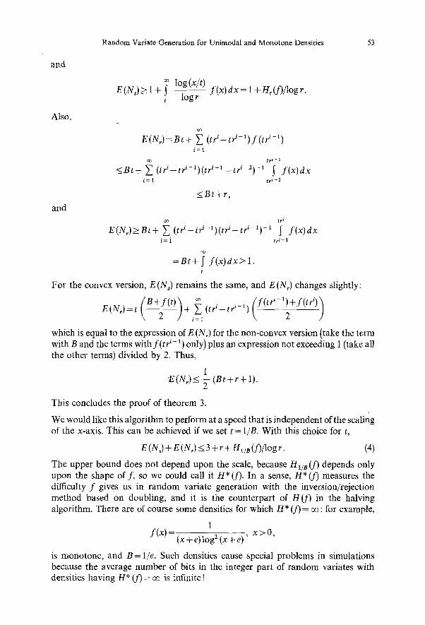
log(x/t) E(Ns)>~ 1 + j f(x)dx= 1 + Ht (f)/log r.

t log r

oo

E(N~)=Bt + ~ (tri-tri-1) f (tri-1) i = ~

t r i - 1

NUt+ ~ (tri-tri-1)(tr i-1 -tri-2) -1 ~ f(x)dx i = i t r i - 2

<_Bt+r,

t r i

E(N~)>_Bt+ ~ (tri-tri-1)(tri-tri-1)-i ~ f(x)dx i = l t r i - 1

=Bt+ ~ f(x)dx>_l. t

For the convex version, E (Ns) remains the same, and E (Nr) changes slightly:

E(N,)=t (B+-f2 (t))+ ~=l (tri_tr~-l) (f(tr'-~)2+ f(tri))

which is equal to the expression of E (N,) for the non-convex version (take the term with B and the terms with f(t/-2) only) plus an expression not exceeding 1 (take all the other terms) divided by 2. Thus,

1 ~(Nr)<_ ~ (Bt +r + 1).

This concludes the proof of theorem 3.

We would like this algorithm to perform at a speed that is independent of the scaling of the x-axis. This can be achieved if we set t = 1lB. With this choice for t,

E (N~) + E (Nr) <_ 3 + r + H~tB (D/log r. (4)

The upper bound does not depend upon the scale, because H1/8 (f) depends only upon the shape o f f , so we could call it H*(f) . In a sense, H*( f ) measures the difficulty f gives us in random variate generation with the inversion/rejection method based on doubling, and it is the counterpart of H (f) in the halving algorithm. There are of course some densities for which H* (f) = oe" for example,

1 f(x) = (x + e) log 2 (x + e) ' x > 0,

is monotone, and B--1/e. Such densities cause special problems in simulations because the average number of bits in the integer part of random variates with densities having H* (J) = ~ is infinite !

54 L. Devroye:

In practice, H*(f) is not known, but other quantities such as E(X) or E (X 2) sometimes are. A loose upper bound for H*(D is afforded by Jensen's inequality:

H* (f)_< ~ log(1 +Bx)f(x)dx<log(1 +E(BX)). 0

Thus, at worst, the average time of the algorithm is logarithmic in E (BX).

Example 1: We continue example 1 of section 3.3, and note that

a + l ' ~ H* ( f ) _<log (1 +E(BX))=log 1 + a~-2)-<l~ all a > 0 .

Thus,

log 2 E (N~) < 1 + r. E (Ns) -< 2 + log r '

The "ad hoc" choice r = 2 makes both upper bounds equal to 3. The average time taken in the algorithm is uniformly bounded in a.

Remark 5: [Choice of r.]

The obvious choice r = 2 gives E (Ns) + E (N,) <_ 5 + H* (D/log 2. The upper bound (4) for E(Ns)+ E(N,) is minimal for the unique value r > 1 for which r log 2 r=H* (D. Copying the discussion of remark 3, we see that the choice r = 2 H* (D/log(H* (f)) makes the upper bound asymptotic to 3 H * (D/log (H * (D) as H * (D--+ oe. Again, this asymptotic rate is better than the one obtained by keeping r fixed: indeed, for r fixed, we have E (N,) + E (N,) > 2 + H* (D/log r. Since/4* (f) is unknown in general, we suggest either estimating it before random variate generation is started (but this would only be feasible if many random variates are needed), or using the value r-- 2.

The inequality H * (D _< log (1 + E (B X)) could help in finding a good value for r when E (BX) is known. For example, by taking

r = 2 log (1 + E (BX))/log log (e + E (BX)) we obtain

E (Ns) + E (N~) _< (3 + o (1))log (E (BX))/log log (E (BX)) as E (BX)--+ oo.

Such a choice of r should be close to the optimal value when the bound H*(f) < log (1 + E (BX)) is tight, i.e. the difference between right and left is small.

3.5. Inversion~Rejection via Newton-Raphson Iterations

In this section, we assume, as in section 3.4, that f is monotone and bounded by B = f ( 0 ) < ~ : f need not have compact support, but both f and F should be computable. The interval search considers the intervals [Xo, xl), [xl, x2), etc. where each x . . 1 is a function of x. only (this avoids the problem of having to store the x.'s), and is computed by the rule

Xn +1 = Xn -[- (1 - - F (x.))/f(x.), x o -- O. (S)


The sequence {x,} thus obtained coincides with the sequence of values obta:fned if we try to solve the equation F (x) = 1 for x by Newton-Raphson iterations started at Xo =0. Since F is concave, we know that x, increases monotonically ~,o a finite solution if it exists, and to oe if no finite solution exists (i.e., f has no compact support). Thus, for 0 < u < 1, the solution of F (x) = u certainly belongs to one of the intervals [x,, x,+ 1).

The advantages of this type of interval search are triple: the average time of the algorithm is scale-invariant; there are no design parameters as for the halving and doubling algorithms; and there is a natural balance between the inversion and rejection steps in the algorithm: E(Ns)= E (Nr) (see theorem 4 below).

Step 1

Step 2 :

Step 3 :

Step 4"

Generate a uniform [0, 1] random variate U, set X ~ 0 . Compute R ~ F ( X ) , Z ~ f ( X ) .

Set X* ~ X + (1 - R)/Z, R* ~ F (X*), Z**-f(X*). If R*> U, go to 3. (The solution of F(x)= U belongs to IX, X*).) Otherwise, R ~ R * , Z*--Z*, X ~ X * , go to 2.

Generate two independent uniform [0, 1] random variates V, W. Set Y ~ X + ( X * - X ) V, T,.- WZ. (Yis uniformly distributed on [-X, X*).)

(Squeeze step. Optional.) If T<Z*, exit with Y. (Acceptance/rejection step.) If T<f (Y ) , exit with Y. Otherwise, go to 3.

Theorem 4 describes a remarkable coincidence: E(Ns)= E (Nr) for all bounded monotone densities. A perfect balance is obtained between the two parts of the algorithm despite the fact that search and rejection are seemingly independent and totally different processes. In other words, on the average, equal amounts of energy are required for the interval search and for the rejection step.

Theorem 4: Let f be a bounded monotone density, and let 0 = Xo <-x I ~ . . . be the sequence obtained by Newton-Raphson iteration (5). Then the inversion~rejection method with Newton-Raphson iterations satisfies

E (Ns) = E (N,) = ~ (1 - F (xi)). i = O

Proof:

and

oo

e(Ns)= i((1-e(x,_,)-(1-e(x,))= Z (1-e(x,)) i = 1 i = 0

i = 0 i = 0

by (5). This concludes the proof of theorem 4.

Formula (5) can be rewritten as

Xn+ 1 --'h'Xn-]- 1/h(x~), X o =0,

56 L. Devroye:

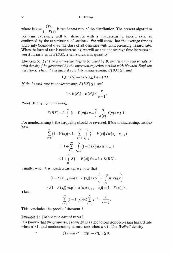
f(x) where h ( x ) - - - is the hazard rate of the distribution. The present algorithm

1 - F (x )

performs extremely well for densities with a nondecreasing hazard rate, as confirmed by the experiments of section 4. We will show that the average time is uniformly bounded over the class of all densities with nondecreasing hazard rate. When the hazard rate is nonincreasing, we will see that the average time increases at worst linearly with E (BX), a scale-invariant quantity.

Theorem 5: Let f be a monotone density bounded by B, and let a random variate X with density f be generated by the inversion/rejection method with Newton-Raphson iterations. Then, if the hazard rate h is nonincreasing, E (BX) > 1 and

1 <E(Nr)=E(Ns)<_ 1 +E(BX).

I f the hazard rate is nondecreasing, E (B X) < 1 and

e

I <-E(Nrl=E(Ns)<e_ 1.

Proof: If h is nonincreasing,

o o ~ f ( x l d x > l .

For nondecreasing h, the inequality should be reversed. If h is nonincreasing, we also have

i(1-F(x'))<l+i -)~ (1-F(x))dx/(xi -x i -1) i=0 i=1 x i 1

= l + i i ' (1 -F(x) )dxh(x i -1) i=1 x i _ 1

_<1+ ~ B ( 1 - F ( x ) ) d x = I + E ( B X ) . 0

Finally, when h is nondecreasing, we note that

(1-F(x i+~))=(1-F(x l ) )exp - ~ h(x)dx

< (1 - F (x)) exp ( - h (x)(xi +1 - x~)) = (1 - F (x~))/e. Thus,

i (1-F(x))_< i e - i - e . i=o i=o e - 1


Example 2: [Monotone hazard rates.] It is known that the gamma (a, 1) density has a monotone nondecreasing hazard rate when a > 1, and nonincreasing hazard rate when a_< 1. The Weibull density

f ( x )=ax a-1 exp(-xa), x > 0 ,


has a nondecreasing hazard for a > 1, and a nonincreasing hazard rate for a_< 1. For the exponential density e -x, x_>0, we have a constant hazard rate 1, so that in (5), xi = i, and thus, ~

E(Nr)=E(Ns)= ( 1 - e ( i ) ) = e_ i= e . i = o i = o e - 1

For a survey of properties of distributions with monotone hazard rates, see Barlow, Marshall and Proschan (1963).

If we continue example 1 of sections 3.3 and 3.4 we see that for the beta (1 , a+ 1) a + l

density (a>O)h(x)= , 0 _ < x < l , which is increasing on [0,1). Thus, 1 - x

e E (N~) = E (Nr) _< for all the examples mentioned above. For the beta (1, a + 1)

e - 1 density, it is easy to derive an exact expression for E (N~) because (5) gives

xo=O.x ,+l=x,(A~)_~ 1 ' a + l '

from which we obtain with some work that x , = 1 - , n_>0. Thus, by theorem 4,

( a ~ i(a+l) 1 E(Ns)=E(N')= ~ (1-F(xi))= ~' (I-x/)"+1= ~ \ a ~ i - ] =- 1 ,+1 ,

, = o

e e which varies from 1 (a =0) to - - as a ~ oe without exceeding - - .

e - 1 e - 1

Consider next the Pareto density f(x) = a/x ~+ 1, x > 1. Here F (x) = 1 - x-a , x_> 1, and h (x) = a/x, x > 1. Also, the parameter a is positive. The bound in theorem 5 for nonincreasing h is very loose as we will see. Clearly, X - 1 is a monotone density bounded by B=a, E(X-1)=(a- l ) -1, a > 1, E(X)~-co, a<_l. But (5) becomes (1) x,+ 1 = xn 1 + , so that x, = 1 + if the search is started at x0 = 1. Thus,

i=0 e

and this varies from (a--,oe), to 2 ( a = 1) and ~ (as a ~ 0) asymptotic to e - 1

For most bounded monotone densities we will recommend inversion/rejection with Newton-Rapbson iterations over inversion/rejection with doubling. Additional speed-ups are possible by storing for example a table of the first K constants (xn, f(x~),F(x,) ) (see remark 1). What is gained in time by the perfect balance E (N~)--E (Nr) usually offsets the loss due the fact that per iteration in the interval search one F computation and one f computation are needed versus only one F computation for the algorithm with doubling.

58 L. Devroye:

3.6. Table Methods

Let f b e a bounded monotone density on [0, 1], and assume that f can be computed but not F. Choose an integer n > 1 and note that f is dominated by 9 where

_<x<-- , i integer, 0___x<_l. g ( x ) = f ' n n

The area under 9 is

c O ( x ) d x = - - f < - - + S B = f (x ) dx = - ~ + 1. (6) 0 1l i= - - n o

where B =f(0) is the bound for f . By choosing n proportional to B (for example, n = B or n=2B). We see that the area under g stays uniformly bounded for all bounded monotone densities on [0, lJ ! In fact, we can make this area as close to 1 as desired by choosing n large enough. Since random variates with density g can be obtained in constant average time by Walker's method (see Walker (1977) or Kronmal and Peterson (1979)), the ordinary rejection method with rejection from g yields a uniformly fast algorithm. In its simplest form, the table method can be summarized as follows.

Step 0: (Set-up.) Compute f ~- , 0 _< i_< n, and store two tables:

Pi = f and q~=f , 1 <i_< n. Let c = - - ~ Pi- n i = i

Compute a table of aliases for Walker's method.

Step 1: Generate an integer I in the range 1 _< I < n where P( I= i )=pJ(cn) by Walker's method. This requires average time bounded by a number that is independent of the pi's.

Generate two independent uniform" F0, 1-] random variates U, V. Set X ~ ( I - 1 + V)/n. (X has density proportional to g.)

Step 2: (Squeeze step. Optional, but recommended.) If U_<ql, exit with X. (Acceptance/rejection step.) If Upr <_f(X), exit with X. Otherwise, go to 1.

Two quantities are of interest here:

1. N r: the number of times that step 1 is executed.

2. Nq: the number of evaluations of f .

Nq is small when the squeeze step is efficient, and Nr is small if the dominating function g is close to fi The average time taken by the algorithm is obviously 0 (E (Nr)). Since the average time is also bounded from below by a constant times E (Nr), we note that the influence of E (Nq) must be limited to reducing the constant.

Theorem 6: Let f be a monotone density on [0, 1] bounded by B. For the table method, we have

B E(Nr)=c<__l + - -

n


and B - 1 B - - <_E(Nq)<_--.

t i 11

Proof: Let f b e a density, let g and h be two nonnegative functions, both integrable, let 0 <_ h <_f<_g, and let the following rejection method be used to generate random variates with density f :

Step 1 : Generate a random variate X with density proportional to g. Generate an independent uniform [0,13 random variate U. Set T~- Ug (X).

Step 2: (Squeeze step.) If T<_h(X), exit with X. (Acceptance/rejection step.) If T<_f(X), exit with X. Otherwise, go to 1.

Then the expected number of executions of step 1 is ~ g, and the expected number of evaluations of f is ~ (g - h), where all the integrals are with respect to dx. Thus, the first statement of theorem 6 follows from (6). The second statement follows from the observation that

i=1 11


When the table method is implemented, we should choose 11 proportional to B; 11 = B to n = 2 0 B seems to be the most useful range. Above n = 2 0 B the storage requirements become prohibitive. Since E (Na)< B/n, we can eliminate the evaluations o f f almost entirely, if we wish. By making 11 large enough, we can reduce the rejection rate at will: the optimal rejection rate of 0~o can be approached. In other words, we are buying time with storage. A fair comparison between variable-storage methods (such as the table method) and fixed-storage methods (such as all the other methods discussed until now) is hardly possible: storage is usually cheap but rather inflexible, while time is expensive but available without limit. If for any physical reason one has to keep 11 smaller than K (say), then in view of E (Nq)> ( B - 1)/n, the average time becomes linear in B just as for the ordinary rejection method but with perhaps a smaller slope.

For the alias method we refer to Walker (1977). The table of n aliases needed in Walker's method can be found in time 0 (11) (Kronmal and Peterson, 1979 a, b). Thus, step 0, the set-up step, requires time proportional to n. In practice, this means that the table method should be avoided in situations in which the number of random variates with the same density is smaller than 11. If the density changes every k random variates for some fixed k, then the average time needed in the algorithm per random variate is bounded by

where ca, c2 > 0 are constants. This is minimized by setting n = ] / ~ Bk/e2, and the upper bound becomes

60 L. Devroye:

c, + c2 S/k

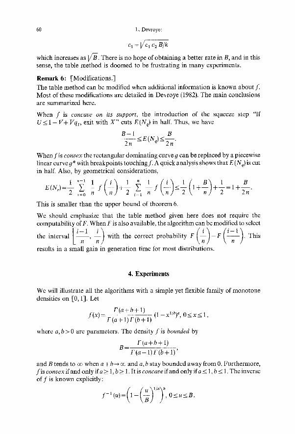
which increases as i//-B. There is no hope of obtaining a better rate in B, and in this sense, the table method is doomed to be frustrating in many experiments.

Remark 6: [Modifications.]

The table method can be modified when additional information is known about f . Most of these modifications are detailed in Devroye (1982). The main conclusions are summarized here.

When f is concave on its support, the introduction of the squeeze step "If U <_ 1 - V+ Vqi, exit with X" cuts E(Nq) in half. Thus, we have

B - 1 B <_E(Nq)<_ 2 "

2n n

When f is convex the rectangular dominating curve g can be replaced by a piecewise linear curve g* with breakpoints touching f . A quick analysis shows that E (Nq) is cut in half. Also, by geometrical considerations,

1 i f +1 i f ( i < 5 1+ n +~- - -=1+- - . , :o - n , : \ n ) - 2 2n

This is smaller than the upper bound of theorem 6.

We should emphasize that the table method given here does not require the computability of F. When F is also available, the algorithm can be modified to select

I i n 1 ; ) ( i ) ( ~ ) the interval , - with the correct probability F - F . This

results in a small gain in generation time for most distributions.

4. Experiments

We will illustrate all the algorithms with a simple yet flexible family of monotone densities on [0, 1]. Let

F ( a + b + l ) f ( x ) - (1 - xl/b) a, 0_<x_< 1,

F ( a + l ) F ( b + l )

where a, b > 0 are parameters. The density f is bounded by

F ( a + b + l) B -

F(a+ l )F(b+ l)'

and B tends to oo when a + b--+ oo and a, b stay bounded away from 0. Furthermore, f i s convex if and only ifa > 1, b > 1. It is concave if and only ifa _< 1, b < 1. The inverse of f is known explicitly:

f - l ( u ) = 1 - , ~ - , O<_u<_B.


An explicit expression for F is only known in special cases, e. g. when a is integer. The

family has many important limiting densities: the normal density = ~ , a ~ oo ,

the exponential density (b-- 1, a ~ oo), the uniform density (a fixed, b J, 0; or b fixed, a ~ 0) and the exPonential power distributions (example 1 of section 3.3: b fixed, a-+oo). Thus, it is flexible enough to be useful in a meaningful comparative experiment.

It is easy to check that X b and have density f , where X, Y and Z are

independent beta (b, a + t), gamma (b, 1) and gamma (a + i, t) random variables respectively. In our experiments, we will only consider the special cases a = 1 and b--1.

Theorem 7: For a = 1, we obtain the density

f ( x ) = ( b + 1)(1 -xl/b), 0_<x_<l,

and the distribution function

F (x)=(b+ l) x - b x 1+1/b, 0<x_< l .

Random variates with this density can be 9enerated as U V b/(b+l) where U, V are

independentuniform [0,1] randomvariates. A s b ~ o v , f ( x ) ~ I o g ( 1 ) , O < x < _ l .

Proof: The first statement follows from Khintchine's theorem (see e.g. Feller (1971), pp. 158) for unimodal random variables. The last statement follows from the inequalities

b + l 1 ( 1 1 ) b + l 1 ~- log 1 - ~ - l o g ~ - _ < f ( x ) _ < - ~ - l o g ~ - , 0_<x< l .

Theorem 8" For b= 1, we obtain the density

f ( x ) = ( a + 1)(1 -x)" , 0 _ < x < l .

The distribution function is F (x) = 1 - (1 - x) "+ :, 0 _< x _< 1. Random variates with this density can be obtained in the following ways:

1. Generate a uniform [0, 1] random variate U, and exit with 1 - U :/("+1).

2. Generate independent exponential and gamma (a + 1, 1) random variates E and X, E

and exit with - - E + X "

3. Rejection form an exponential density:

Step 1: Generate two independent exponential random variates EDE 2. Set X ~ E1/a. I f X > l, 9o to 1.

Step 2: I f E 2 ( 1 - X ) - a X 2 > _ O , exit with X .

Step 3 : I f a X + E 2 +a log(1 - X ) > 0 , exit with X. Otherwise, 90 to 1.

62 L. Devroye:

4. Rejection from a uniform density:

Step 1: Generate two independent uniform [0, 1] random variates U, X.

Step 2: I f U_<(1-X) a, exit with X. Otherwise, go to 1.

a + l The average number of executions of step 1 in method 3 is - - , and the average

a

number of executions of step 1 in method 4 is a + 1. These average numbers are equal when a= 1. The method that combines method 3 for a> 1 with method 4 for a< 1 has uniformly bounded average time; step 1 is guaranteed to be executed at most 2 times on the average.

Proof: No explanation is required, except for method 3, which is based on the inequalities

exp ( - a x / ( 1 - x ) ) <(1-x)a_<exp(-ax) , 0_<x_< 1.

The different methods were coded in FORTRAN and compared on McGill University's AMDAHL V7 computer. For uniform [0, t] and exponential random variates, we used subprograms UNI and REXP of the "Super-duper" random number generator package. Only the density f given in the previous section was considered. The parameters a and b were varied as follows:

Experiment 1: a = l , b=2i/10, i=2, ..., l l .

Experiment 2: b = 1, a = 2i/10, i-- 2,..., 11.

In all these cases, f is either convex or concave. Also, f has support [0, 1] and is bounded by B = ( b + l ) in Experimentl, and by B = ( a + l ) in Experiment2. Necessary constants and tables are computed in separate set-up subprograms, and the density f or distribution function F is always passed as a parameter. The parameter passing slows the algorithms down, so that all the timings given here are pessimistic. No attempt was made to subtract the time due to overhead costs in subprogram calls. For each algorithm we will give:

1. The average time per random variate in microseconds. The average is obtained by repeating the experiment n times where n varied between 200 (for slow methods) and 5000 (fast methods). The results still have some residual variation, but we are not interested here in obtaining accurate times, but rather in detecting trends and making global comparisons.

2. The set-up time needed to compute all constants and tables.

3. The size of the compiled program (in bytes).

4. The size of a variable size table (in entries, or words).

For the FORTRAN programs we refer to Devroye (1982): these are available from the author upon request. The algorithms are given symbolic names in the tables:

D 1 : direct method 1 : method 1 of theorem 8 for case b-- 1.

D2: direct method 2: method 2 of theorem 8, with gamma variate generation by Marsaglia's squeeze method (Marsaglia, 1977). Case b = 1 only.


D3" direct method 3: the combina t ion of rejection method 3 and rejection

method 4 of theorem 8. Case b = 1 only.

D4: direct method 4: the t ransformation-of-uniforms method suggested in

theorem 7. Case a = 1 only.

D5: direct method 5: same as D4, but instead of UP/(b+l), we use U exp ( - Eb/(b + 1)) where U is uniform [0, 1] and E is exponential . Case a = 1

only.

I: inversion method using Newton-Raphson iterations. See section 3.1.

R 1" ordinary rejection method with rectangular domina t ing function.

R2: modified rejection method as described in section 3.2.

1 I R I : inversion/rejection method with halving, r = t 2 ' see section 3.3.

IR2: inversion/rejection method with doubling, t = l/B, r = 2, see section 3.4.

1R3: inversion/rejection method with Newton-Raphson iterations. See section 3.5.

IR4: inversion/rejection method with halving, safe value for r.

1R5: inversion/rejection method with doubling, safe value for r.

T(n): table method with table size int(nB). Only values n = 1 , 5 and 20 are considered here. See section 3.6.

The direct methods are all uniformly fast over the variable parameters. They should not be considered as competitors, but as s tandards against which other perfor- mances are gauged. Our experiment demonstrates that no method except possibly the inversion method is strictly domina ted by some other method in all respects. The inversion method seems domina ted by the inversion/rejection method with Newton-Raphson iterations because the costly refinement is done by rejection in the latter method.

Table 1. Average times in experiment 1 as the parameter a varies from 22/10 to 2~/10

D 1 41.6 41.8 41.6 41.8 41.7 41.7 4l .8 41.5 42.0 41.7 D2 44.7 43.4 44.3 43.5 43.2 41.3 4l .2 43.2 40.7 41.3 D3 57.7 70.2 43.1 38.4 33.6 32.0 30.5 30.4 29.9 29.7

I 375.5 392.3 405.7 415.1 436.5 466.0 465 .4 521.3 492.3 503.3 R1 70.7 83.5 128.9 187.7 341.9 596.4 1121 1836 4873 9310 R2 74.1 81.8 87.1 93.3 102.2 114.4 105.2 115.6 114.3 114.1 IR 1 179.1 209 .2 234.5 255.9 302.8 332.5 347.5 379.5 415.9 449.3 IR2 210.1 208 .7 243.5 257.0 254.1 232.4 251.1 264.0 246.9 242.0 IR3 157.2 167.2 178.2 186.8 186.5 203.5 200.9 193.8 197.7 190.8 IR4 168.2 197.4 236.9 242.6 261 .2 282.5 300.0 307.9 360.9 390.9 IR5 202.9 274.2 242 .4 254.7 259.5 272 .4 275.6 318.7 272.2 308.2 T(1) 73.8 73.8 100.2 86.8 87.8 86.3 89.4 87.3 88.7 88.5 T(5) 48.2 49.4 48.2 49.3 47.5 47.9 48.2 48.0 48.1 48.4 T(20) 40.8 40.9 40.8 41.9 41.0 40.9 41.7 41.5 - -

64 L. Devroye:

Table 2. Average times in experiment 2 as the parameter b varies from 22/10 to 2 z 1/10

D4 45.3 45.3 45.3 45.4 45.3 45.3 45.3 45.3 45.4 45.3 D5 34.2 34.4 34.1 35.1 35.3 34.4 34.4 34.5 34.7 34.2

I 292.1 3 4 7 . 1 3 7 8 . 3 4 2 8 . 5 4 5 5 . 5 461.7 4 8 4 . 3 4 9 1 . 1 4 9 1 . 5 496.7 R1 73.1 85.6 138 .1 1 8 8 . 3 3 7 6 . 6 634 .6 1075 2028 4281 10100 R2 75.8 82.1 91.2 95.2 1 0 2 . 1 1 0 6 . 9 1 0 3 . 0 113 .1 1 1 6 . 3 118.4 IR 1 205.4 2 1 9 . 4 231.4 2 3 8 . 7 2 4 7 . 9 2 3 8 . 7 253.2 2 6 2 . 2 2 6 4 . 4 259.5 IR2 157.1 1 8 0 . 8 2 0 6 . 2 2 2 3 . 6 2 5 0 . 7 2 9 3 . 9 3 1 5 . 6 3 4 2 . 7 3 7 8 . 2 398.9 IR3 127.3 1 4 0 . 7 162 .0 198 .5 2 2 8 . 6 2 4 9 . 5 2 6 1 . 3 2 9 3 . 5 2 9 9 . 9 299.2 IR4 182.6 206.4 2 2 1 . 3 2 2 5 . 1 220.2 2 3 1 . 5 2 3 5 . 5 2 2 5 . 8 2 4 8 . 8 2372 IR5 161.8 224 .1 2 1 0 . 8 238.4 2 6 2 . 0 2 8 5 . 8 3 1 6 . 4 3 3 0 . 8 3 4 8 . 7 372.3 T(1) 73.7 73.7 100.1 86.0 80.2 74.2 69.4 66.5 69.1 64.6 T(5) 48.3 49.7 47.9 48.8 46.3 46.1 45.8 46.4 45.1 44.5 T(20) 40.9 40.9 40.7 41.5 40.6 40.8 40.2 40.6 - -

Table 3. Properties of the various algorithms

Average set-up Average set-up Program size Set-up program Table size time experiment 1 time experiment 2 (bytes) size (bytes) (words)

D 1 0 - 402 0 0 D2 0 - 8 6 4 0 0

D 3 0 - 650 0 0 D4 - 0 422 0 0 D5 - 0 416 0 0 I 0 0 642 0 0 R 1 51 26 470 376 0 R2 71 51 794 498 0 IR 1 0 0 632 0 0 1R2 0 0 686 0 0 IR3 0 0 718 0 0 IR4 70 50 654 474 0 IR5 70 50 708 508 0 T(1) 275.8 + 50.5 B in both experiments 850 2142 int (B) T(5) 244.6 + 257.8 B in both experiments 850 2142 int (5 B) T(20) 249.0 + 1142.3 B in both experiments 850 2142 int (20 B)

Tab le s 1 a n d 2 s h o w the a v e r a g e t imes pe r r a n d o m var i a t e for E x p e r i m e n t s 1 a n d 2

respect ive ly . T a b l e 3 shows the o t h e r fac tors : the ave r age se t -up t ime, the size of the

c o m p i l e d p r o g r a m , a n d the t ab le size. All the p r o g r a m s t ake b e t w e e n 402 and 864 bytes (with an ex t ra 376 to 508 bytes for se t -up p r o g r a m s wi th the excep t ion of the se t -up p r o g r a m for the tab le m e t h o d , wh ich requ i res 2142 bytes). Thus , excep t for

the tab le m e t h o d , the p r o g r a m size is n o t an i m p o r t a n t e n o u g h issue for dec id ing

b e t w e e n a lgo r i t hms . T h e t rue d i f fe ren t ia t ion m u s t be m a d e on the basis of such

factors as speed and flexibili ty.

Direc t m e t h o d s

O f the d i rec t m e t h o d s , D 3 is faster t h a n D 1 a n d D 2: D 1 uses cos t ly o p e r a t i o n s all the t ime, and D 2 is ind i rec t because we t r a n s f o r m g a m m a r a n d o m var ia tes . S ince the


original density f i s simpler than the gamma density, such an indirect route can only lead to slowdowns.

D 5 is faster than D 4 because exponential random variates are generated faster than a logarithm is computed. This order may be reversed elsewhere.

Inversion method

In both experiments, the average time of the inversion method increases with B. No theoretical analysis of the average time was given in this paper because we wanted to avoid the messy issue of stopping times (should we stop when the absolute error is small, or when the relative error is small; and how are the errors obtained ?). Such an analysis would be a waste of time because the method is obviously slower than all the other methods. In addition, it is the only non-exact method among all the methods considered here.

Rejection methods

The average times for R 1, R2 are linear respectively logarithmic in B as was predicted by our analysis. The simple modification gives a dramatic improvement in performance. The improvement was so extraordinary that for the range of parameter values considered here, the modified rejection method was the fastest fixed storage method (the table method being the only variable storage method). It is recommended whenever f is monotone, bounded, and f has compact support. For unbounded monotone densities with unbounded support, we recommend a combination of several methods by partitioning the interval [0, oe) into [0, 1] and [1, oe). For convex f (columns3 through 10 in Tables l, 2), we coded the improvement suggested in section 3.2, and obtained average times that varied from 80.5 (3rd column) to 102.5 (10th column). This is a 10~ to 20~o gain in average time.

Inversion~rejection methods

In all cases, we used the original algorithms of sections 3.3-3.5. None of the modifications suggested for convex or concave densities were implemented. From Examples 1 and 2 of sections 3 .3-3.5 we recall that the average time in Experiment 1 increases as log (B) for IR 1, and remains uniformly bounded for 1R 2 and IR3. This trend is observed in Table 1. In fact, IR3 is faster than IR2 which in turn is faster than IR1. IR2 and IR3 have similar left-to-right interval search components. Because of the perfect balance achieved by IR3, we expect IR3 to almost always perform better than IR2. The comparison with IR 1 is not so straightforward, and it is for this reason that we choose to include Experiment 2 in this paper. For the density in Experiment 2 we have by elementary Taylor series inequalities

b 2b

0<x_<l .

5 Computing 32/1

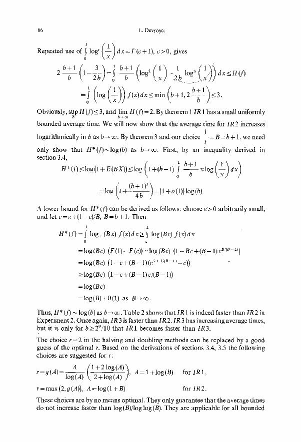
66 L. D e v r o y e :

Repeated use o r s log c dx=F(c+l) , c>0, gives

( 3 ) 1 b + l (1 ( 1 ) 1 3 @ ) ) 2 b + l 1 - ~ - = ! ~ - og 2 -~__ log dx<_H(f) b 7 . . . .

b + l \ =i O o g ( 1 ) ) f ( x ) d x < - m i n ( b + l , 2 ~ - ) < - 3.

Obviously, sup H (f) _< 3, and lim H (f) = 2. By theorem 1 IR 1 has a small uniformly b b~co

bounded average time. We will now show that the average time for IR 2 increases 1

logarithmically in b as b ~ oo. By theorem 3 and our choice - - = B = b + 1, we need t

only show that H*(f )~log(b) as b~oe . First, by an inequality derived in section 3.4,

o b

(b + 1) 2 , = log ( t + ~ - ) = (1 + o (1)) log (b).

A lower bound for H*(f) can be derived as follows: choose e > 0 arbitrarily small, and let c = e + ( 1 - e ) / B , B=b+ 1. Then

1 1

H*(f) = j" log+ (Bx) f ( x )dx> ~ log(Bc) f (x )dx 0 c

= log (B c) (F (1) - F (c)) = log (Be) (1 - B c + (B - 1) c B/(B- ~))

=log(Bc) ( 1 - c + ( B - 1)(C1+1/(B-1)--C))

> log (Be) (1 - c + (B - 1) c/(B - 1))

=log(Be)

=log(B)+0(1) as B~oo .

Thus, H* (f) ~ log (b) as b --, oo. Table 2 shows that IR 1 is indeed faster than IR 2 in Experiment 2. Once again, IR 3 is faster than IR 2. IR 3 has increasing average times, but it is only for b>29/10 that IR1 becomes faster than IR3.

The choice r---2 in the halving and doubling methods can be replaced by a good guess of the optimal r. Based on the derivations of sections 3.4, 3.5 the following choices are suggested for r:

A ~1 +2 log(A)) r = g (A) = log (A) \ 2 + log (A) ' A = 1 + log (B) for IR 1,

r=max(2,g(A)), A=log(1 +B) for IR2.

These choices are by no means optimal. They only guarantee that the average times do not increase faster than log (B)/log log (B). They are applicable for all bounded


monotone densities because we can take B =f(0). An improvement is expected for large values of B for those methods for which H (f) or H* (f )~ o0 as B ~ oe (1R 1 in Experiment 1, IR2 in Experiment 2). A worsening is expected for the other cases, because a uniformly bounded average time is replaced by an unbounded average time increasing as log (B)/log log (B). These observations are corroborated by the timings for IR4 and IR5 in Tables 1 and 2.

Table methods

All the algorithms T(n) have uniformly bounded average times. Very little improvement is possible beyond n = 20. It is pleasing to see that we can approach the average times of the direct methods albeit by paying rather heavily in terms of storage (see Table 3). If we fix the table size, then the average time becomes linear in B. None of the improvements suggested in section 3.6 were implemented.

The rejection and table methods can only be used for bounded monotone densities with compact support, but they do not require the availability of F. The ordinary rejection method can in fact be considered as a table method with table size 1. It goes without saying that table methods should only be used when the density changes infrequently because of the prohibitive set-up times involved.

We conclude by noting that in terms of flexibility, the inversion/rejection methods have no competition: a suitable combination of two of them can be used for all monotone densities. The halving method takes care of the peak at 0 while the doubling method or the Newton-Raphson iterations could be used to handle infinite tails. The only restriction is that both f and F must be computable.

Acknowledgement

The author acknowledges the helpful suggestions of one referee.

References

Ahrens, J. H., Kohrt, K. D. : Computer methods for efficient sampling from largely arbitrary statistical distributions. Computing 26, 19-31 (1981).

Barlow, R. E., Marshall, A. W., Proschan, F. : Properties of probability distributions with monotone hazard rate. Annals of Mathematical Statistics 34, 375-389 (1963).

Chen, H. C., Asau, Y.: On generating random variates from an empirical distribution. AIIE Transactions 6, 163-166 (1974).

Devroye, L. : Random variate generation for unimodal and a'nonotone densities. Technical Report, School of Computer Science, MeGill University, Montreal, Canada H3A 2K6, 1982.

Feller, W. : A n Introduction to Probability Theory and Its Applications, Vol. 1. New York: J. Wiley 1961.

Feller, W. : An Introduction to Probability Theory and Its Applications, Vol. 2, 2rid ed. New York: J. Wiley 1971.

Hardly, G. H., Littlewood, J. E., Polya, G. : Inequalities, 2nd ed. London: Cambridge University Press 952.

Kohrt, K. D. : Efficient sampling from non-uniform statistical distributions. Diploma Thesis, University of Kiel, Federal Republic of Germany, 1980.

Kronmal, R. A., Peterson, A. V. : On'the alias method for generating random variables from a discrete distribution. The American Statistioian 33, 214 - 218 ( 1979 a).

5*

68 L. Devroye: Random Variate Generation for Unimodal and Monotone Densities

Kronmal, R. A., Peterson, A. V. : Programs for generating discrete random integers using Walker's alias method. Manuscript, Department of Biostatistics, University of Washington, Seattle, Washington, 1979b.

Marsaglia, G. : The squeeze method for generating gamma variates. Computers and Mathematics with Applications 3, 321-325 (1977).

Schmeiser, B. W. : Random variate generation: a survey. Proceedings of the 1980 Winter Simulation Conference, Orlando, Florida, 1980.

Steffensen, J. F. : On certain inequalities between mean values and their application to actuarial problems. Skand.Aktuarietidskrift 1, 82 -97 (1918).

Steffensen, J. F. : On a generalization of certain inequalities of Tchebychef and Jensen. Skand. Aktuarietidskrift 8, 137-147 (1925).

Walker, A. J. : An efficient method for generating discrete random variables with general distributions. ACMTransactions on Mathematical Software 3, 253-256 (1977)

Prof. Dr. L. Devroye School of Computer Science McGill University 805 Sherbrooke Street West Montreal, P.Q. Canada, H3A 2K6

Documents

Random variate generation for unimodal and monotone …luc.devroye.org/devroye-unimodal+monotone.pdf · Random Variate Generation for Unimodal and Monotone Densities ... can be obtained