Embed Size (px)
Citation preview
Journal of Statistical Planning andInference 135 (2005) 165–196
www.elsevier.com/locate/jspi
Random walks in octants, and related structures
Heinrich NiederhausenDepartment of Mathematical Science, Florida Atlantic University, Boca Raton, FL 33431, USA
Received 10 October 2002; received in revised form 20 March 2003; accepted 7 February 2005Available online 23 March 2005
Abstract
A diffusion walk inZ2 is a (random) walk with unit step vectors→, ↑,←, and↓. Particles fromdifferent sources with opposite charges cancel each other when they meet in the lattice. This cancel-lation principle is applied to enumerate diffusion walks in shifted half-planes, quadrants, and octants(a three-dimensional version is also considered). Summing over time we calculate expected numbersof visits and first passage probabilities. Comparing those quantities to analytically obtained expres-sions leads to interesting identities, many of them involving integrals over products of Chebyshevpolynomials of the first and second kind. We also explore what the expected number of visits meanswhen the diffusion in an octant is bijectively mapped onto other combinatorial structures, like pairsof non-intersecting Dyck paths, vicious walkers, bicolored Motzkin paths, staircase polygons in thesecond octant, and{→↑}-paths confined to the third hexadecant enumerated by left turns.© 2005 Elsevier B.V. All rights reserved.
MSC:primary 60J15; secondary 05A15; 05A19
Keywords:Random walks; Lattice path enumeration; First passage
1. Introduction
There are many applications and therefore many names for random walks in the squareinteger latticeZ2 with unit step vectors→, ↑,←, and↓; we will call them diffusion walksbecause of the fruitful physical interpretation of the walkers as particles spreading out froma source and being able to interact with particles coming from other sources. We find this“cancellation principle” of particles of opposite charges a better model for enumerationthan the frequently applied “reflection principle” . For example, let us starttwo diffusion
E-mail addresses:[email protected], [email protected].
0378-3758/$ - see front matter © 2005 Elsevier B.V. All rights reserved.doi:10.1016/j.jspi.2005.02.013
166 H. Niederhausen / Journal of Statistical Planning and Inference 135 (2005) 165–196
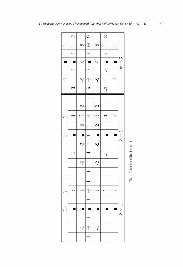
processes at the same time, one from the source⊕ at the origin, and a negatively chargedsynchronous diffusion from the source� at the “mirror” location(−2l,0), wherel is apositive integer. The diagrams inFig. 1 show the location of the sources and the number ofways a particle can reach a lattice point afterk= 1,2,3 steps. The walks from the (virtual)negative source are counted as negative numbers; they annihilate thewalks from the positivesource when reaching the boundary linex = −l. Thus the boundary is absorbing, and noparticle that visits a point to the right of it has ever been to the boundary.Only eight such sources, four positive and four negative, are needed to keep the diffusion
inside a shifted octant, to the right ofx =−l and strictly abovey = x − d (seeFig. 3). Thiswill explain why the expression for the number of such diffusion walks from the origin to(n,m) in m+ n+ 2k steps in the second octant (whenl = d = 1) is so simple,
(n+ 1)(2+m)(m+ 3+ n)(m+ 1− n)
6(n+ k + 1)(n+m+ 2k + 2
n+ k
)
×(n+m+ 2k
k
)/(n+m+ k + 3
3
).
To show how the complexity increases if the cancellation principle is applied in threedimensions, we solve a generalization of the above problem, the enumeration of three-dimensional (3-D) diagonal diffusion with eight step vectors(±1,±1,±1)when the walksstay in the conez�y�x�0. Instead of 8 we need 48 sources; the formula is given inSubsection 2.3.1, Eq. (12). A special case of that formula is the number of walks returningto the origin in 2k steps,
20CkCk+1Ck+2/((
k + 53
)(k + 43
)), (1)
whereCk stands for thekth Catalan numbers.There are several statistics on walks in octants that lead to combinations of Catalan
numbers, likeC (k+1)/2�C 1+k/2� in (8), the relatedCkCk+1 in (10), andCkCk+2−C2k+1 in(11). Thus diffusion in an octant is only one of several visualizations of the same (unnamed)underlying combinatorial structure; they all deserve attention, but we will mention only afew in Section 4 on related structures,
• pairs (and triples) of non-intersecting Dyck paths (and three vicious walkers),• bicolored Motzkin paths,• staircase polygons in the (augmented) second octant, and• {→↑}-paths in the (augmented) third hexadecant enumerated by left turns(omitting Young tableaux (Gouyou-Beauchamps, 1986), and skew Ferrer’s diagrams
(Delest and Fedou, 1993)).The physical approach (diffusion of particles) has a long history; a wealth of results can
be found inRandom paths in two and three dimensionsby McCrea and Whipple (1940).Via the expected numberE(n,m) of visits to (n,m) they found numerous first passageprobabilities for random walks in a rectangle by solving the difference equationE(n,m)=14(E(n− 1,m)+E(n+ 1,m)+E(n,m− 1)+E(n,m+ 1)). The cancellation principle
H. Niederhausen / Journal of Statistical Planning and Inference 135 (2005) 165–196 167
Fig.1.Diffusionrightofx=−r
168 H. Niederhausen / Journal of Statistical Planning and Inference 135 (2005) 165–196
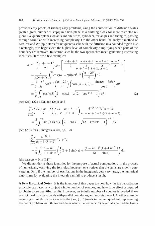
provides easy proofs of (hence) easy problems, using the enumeration of diffusion walks(with a given number of steps) in a half-plane as a building block for more restricted re-gions like quarter planes, octants, infinite strips, cylinders, rectangles and triangles, passingthrough formulae with increasing complexity. On the other hand, the analytic method ofMcCrea andWhipple starts for uniqueness sake with the diffusion in a bounded region likea rectangle, thus begins with the highest level of complexity, simplifying when parts of theboundary are removed. In Section 3 we let the two approaches meet, generating interestingidentities. Here are a few examples:
4−m−l(m+ l − 1
m
)4F3
[m+ l + 2
2,m+ l + 1
2,m+ l + 1
2,m+ l
2;
m+ l + 1, l + 1,m+ 11
]
= l
�(m+ l)
∫ �
0cos((m− l)�)cotl+m
(�+ 2�4
)d�
= 1
2�
∫ �
0cotm+l
(�+ 2�4
)(cos((m− l)�)− sin((m− l)�)
cos�
)d�
= 1�
∫ �
0cos(m�)
(2− cos�−
√(2− cos�)2− 1
)ld� (2)
(see (21), (22), (23), and (24)), and
∞∑k=0
(2k +m+ l
k
)(2k +m+ l + 1k + 1+m
)4−2k−m−l l(m+ 1)
(k +m+ l + 1)(2k +m+ l)
= 2�
∫ �
0sin(lx) sin(x)
(2− cosx −
√(2− cosx)2− 1
)m+1dx
(see (29)) for all integersm�0, l�1, or
6∞∑k=0
4−2k−1
(k + 3)(k + 2) Ck+1Ck
= 1�
∫ �
0
1− sinx1+ sinx
(1
3(1+ 5 sin(x))+ (1− sinx)2(1+ 4 sin2x)
5(1+ sinx)
)dx
(the casem= 0 in (31)).We did not derive these identities for the purpose of actual computations. In the process
of numerically verifying the formulas, however, one notices that the sums are slowly con-verging. Only if the number of oscillations in the integrands gets very large, the numericalalgorithms for evaluating the integrals can fail to produce a result.
A Few Historical Notes. It is the intention of this paper to show how far the cancellationprinciple can carry us with just a finite number of sources, and how little effort is requiredto obtain those beautiful results. However, aninfinite number of sources is needed if werestrict thediffusion to bandswith parallel boundaries, and subsets thereof.Another examplerequiring infinitely many sources is the{←,↓,↗}-walk in the first quadrant, representingthe ballot problem with three candidates where the winner (↗) never falls behind the losers
H. Niederhausen / Journal of Statistical Planning and Inference 135 (2005) 165–196 169
(←,↓) during the counting of the votes (Kreweras, 1965). There is a wealth of approachesto the enumeration of walks bounded by hyperplanes, some of them attacking the problem(including all those with binomial results in this paper) from a very general angle (Gesseland Zeilberger, 1992; Biane, 1992), or considering different kinds of boundary conditionsand step sets (Niederhausen, 2002). In a recent paper,Bousquet-Mélou (2002)applies thekernel methodto “Counting Walks in the Quarter Plane”. Of course, these few referencescannot even scratch the surface of the mountain of literature that has accumulated on thetopic of planar walks; the situation gets worse when we discuss related structures in Section19. Some references can be found in Janse van Rensburg’s book (Janse van Rensburg,2000) and a few others are interspersed among the results in Section 19. Mohanty’s bookon “Lattice Path Counting and Applications” (Mohanty, 1979) is still a valuable resourcefor a first introduction to that topic.
2. Restricted diffusion
If the diffusion has only one source⊕, at the origin, say, and no restrictions, then thenumberUk(n,m) of ways a particle can reach the point(n,m) in k steps is
Uk(n,m)=(
kk + n+m
2
)(k
k + n−m
2
). (3)
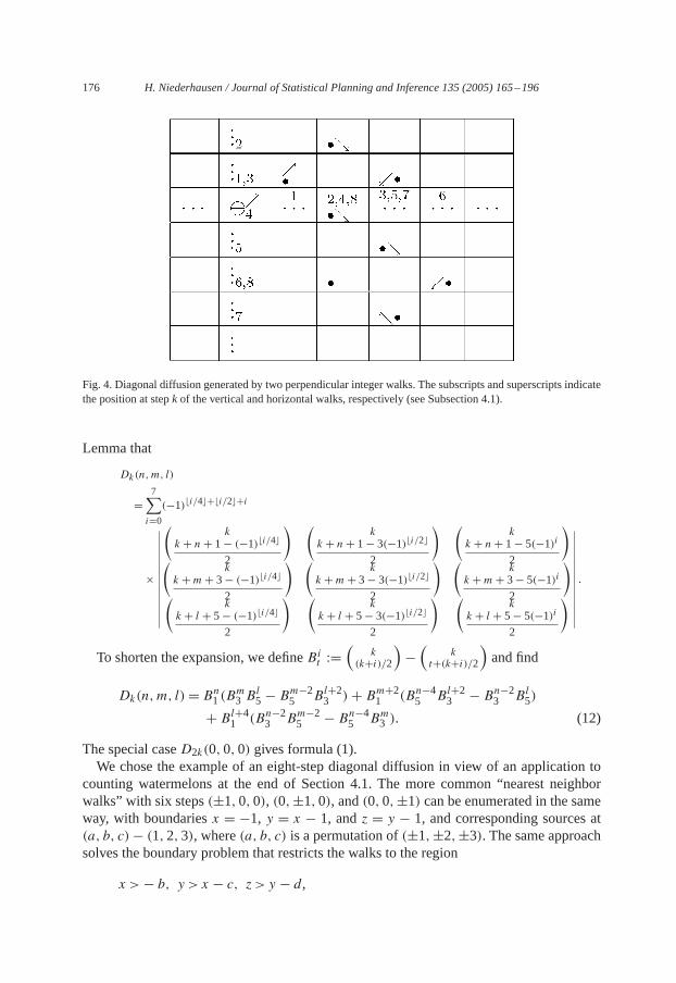
This is of course well-known; for a proof by picture seeFig. 4. No particle can reach(n,m)
in ksteps ifk+n+m is odd, or|n|+|m|>k; wemust interpret the binomial coefficient(ij
)as 0 if i or j are fractions or negative integers. Note the four axes of symmetry in diffusionwalks: thex-axis,y-axis, and the diagonalsy =±x. Thus
Uk(n,m)= Uk(|n|, |m|)= Uk(|m|, |n|).Stirling approximation shows that for largek the walk ends at(n,m) after 2k + |n| + |m|steps with probability approximately(�k)−1. Hence the expected number of visits to(n,m)is infinite.We begin with a review of well known results in the enumeration of diffusion walks
restricted to half- and quarter-planes. The pictures we show are not proofs in the strictsense; they are a suggestive “physical interpretation”, based on the cancellation principle.However, the answers they suggest can be easily verified by checking the recursion andinitial values. Another iteration of the “method of images” or cancellation principle leadsfrom walks in quadrants to octants in Subsection 2.3. A more algebraic than geometric wayof applying the cancellation principle is shown in Subsection 2.3.1.
2.1. Half-planes
Supposel is a positive integer. As a prototype of diffusion restricted to half of the latticewe count the walks strictly to the right of theleft boundaryx =−l. We starttwodiffusionprocesses at the same time, one from the source⊕ at the origin, and a synchronous nega-tively charged diffusion from the source� at the mirror location(−2l,0). The diagrams
170 H. Niederhausen / Journal of Statistical Planning and Inference 135 (2005) 165–196
in Fig. 1show the location of the sources and the number of walks afterk = 1,2,3 steps.The walks from the (virtual) negative source are counted as negative numbers; they annihi-late the walks from the positive source when reaching the boundary linex =−l. Thus thenumberHl|
k (n,m) of walks in a Half plane to(n,m) from the origin ink� |n| + |m| stepsstrictly to the right of the linex =−l is
Hl|k (n,m)= Uk(n,m)− Uk(n+ 2l, m)
=(
kk+n+m2
)(k
k+n−m2
)−(
kk+n+m2
+l)(
kk+n−m2
+l).
(4)
The casel = 1 shows that forn�0
H1|2k+n+|m|(n,m)=
n+ 12k + n+ |m| + 1
(2k + n+ |m| + 1
k
)(2k + n+ |m| + 1
k + |m|)
walks reach(n,m) in 2k + n+ |m| steps staying strictly in the right half plane.Denote the number of walks to(n,m) strictly left of x = r byH |rk (n,m). By symmetry,
H|rk (n,m) = H
r|k (−n,m). For more results on two-dimensional random walks in general
seeCsáki (1997); for diffusion in a quadrantGuy et al. (1992), and for planar walks insidea rectangleNiederhausen (1998).
2.2. Quadrants
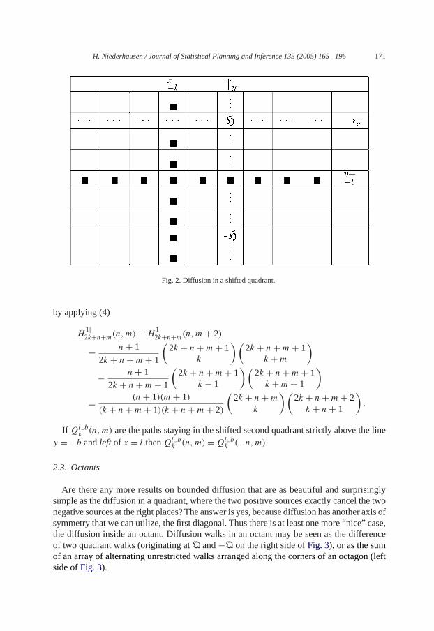
If we want the diffusion to stay in the shifted first quadrant (aquadrant walk) strictlyabove the bottom liney=−b and right ofx=−l we only have to study the scheme inFig.2.One negative sourceH of a virtual walk in the half-planex� − l is needed to cancel
alongy =−b the same type of half-plane walk from the origin. Letn>− l andm>− b.Thus
Ql�bk (n,m) := H
l|k (n,m)−H
l|k (n,m+ 2b)
is the number of quadrant walks from the origin to(n,m) in ksteps. Note thatQl�bk (n,m)=
Qb�lk (−m,−n).The diagram also shows thatQl�b
k (n,m) := Hl|k (n,m) − H
l|k (n,m − 2b) whereQl�b
enumerates fourth-quadrant walks strictly right ofx = −l and belowy = b. Note that form>0
Ql�bk (n,m− b)=H
l|k (n, b −m)−H
l|k (n,−m− b)=Ql�b
k (n, b −m).
For l = b = 1 we obtain the number[(n + 1)(m + 1)/((k + n + m + 1)(k + n + m +2))](2k+n+m
k
) (2k+n+m+2k+n+1
)of quadrant walks to(n,m) ∈ N20 in 2k + n + m steps,
H. Niederhausen / Journal of Statistical Planning and Inference 135 (2005) 165–196 171
Fig. 2. Diffusion in a shifted quadrant.
by applying (4)
H1|2k+n+m(n,m)−H
1|2k+n+m(n,m+ 2)
= n+ 12k + n+m+ 1
(2k + n+m+ 1
k
)(2k + n+m+ 1
k +m
)
− n+ 12k + n+m+ 1
(2k + n+m+ 1
k − 1)(2k + n+m+ 1
k +m+ 1)
= (n+ 1)(m+ 1)(k + n+m+ 1)(k + n+m+ 2)
(2k + n+m
k
)(2k + n+m+ 2
k + n+ 1).
If Ql�bk (n,m) are the paths staying in the shifted second quadrant strictly above the line
y =−b andleft of x = l thenQl�bk (n,m)=Ql�b
k (−n,m).
2.3. Octants
Are there any more results on bounded diffusion that are as beautiful and surprisinglysimple as the diffusion in a quadrant, where the two positive sources exactly cancel the twonegative sources at the right places?The answer is yes, because diffusion has another axis ofsymmetry that we can utilize, the first diagonal. Thus there is at least one more “nice” case,the diffusion inside an octant. Diffusion walks in an octant may be seen as the differenceof two quadrant walks (originating atQ and−Q on the right side ofFig. 3), or as the sumof an array of alternating unrestricted walks arranged along the corners of an octagon (leftside ofFig. 3).
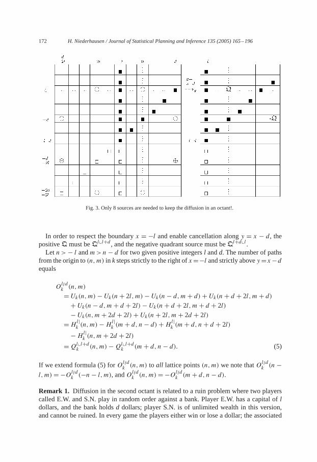
172 H. Niederhausen / Journal of Statistical Planning and Inference 135 (2005) 165–196
Fig. 3. Only 8 sources are needed to keep the diffusion in an octant!.
In order to respect the boundaryx = −l and enable cancellation alongy = x − d, thepositiveQ must beQl�l+d , and the negative quadrant source must beQl+d�l .Let n>− l andm>n− d for two given positive integersl andd. The number of paths
from the origin to(n,m) in ksteps strictly to the right ofx=−l and strictly abovey=x−dequals
Ol|/dk (n,m)
= Uk(n,m)− Uk(n+ 2l, m)− Uk(n− d,m+ d)+ Uk(n+ d + 2l, m+ d)
+ Uk(n− d,m+ d + 2l)− Uk(n+ d + 2l, m+ d + 2l)− Uk(n,m+ 2d + 2l)+ Uk(n+ 2l, m+ 2d + 2l)
=Hl|k (n,m)−H
l|k (m+ d, n− d)+H
l|k (m+ d, n+ d + 2l)
−Hl|k (n,m+ 2d + 2l)
=Ql�l+dk (n,m)−Ql�l+d
k (m+ d, n− d). (5)
If we extend formula (5) forOl|/dk (n,m) to all lattice points(n,m) we note thatOl|/d
k (n −l, m)=−Ol|/d
k (−n− l, m), andOl|/dk (n,m)=−Ol|/d
k (m+ d, n− d).
Remark 1. Diffusion in the second octant is related to a ruin problem where two playerscalled E.W. and S.N. play in random order against a bank. Player E.W. has a capital ofldollars, and the bank holdsd dollars; player S.N. is of unlimited wealth in this version,and cannot be ruined. In every game the players either win or lose a dollar; the associated
H. Niederhausen / Journal of Statistical Planning and Inference 135 (2005) 165–196 173
diffusion walk takes a stepto the East,→, if E.W. wins, to the West,←, if E.W. loses,to the South,↓, if S.N. wins, and to the North,↑, if S.N. loses.Player E.W. is ruined when his capital is down to zero; the same holds for the bank. Thus
Ol|/dk (1− l, m) is the number of ways gambler E.W. can get ruined ink + 1 games whenplayer S.N. has a gain (or loss) ofmdollars. The banker can get ruined inOl|/d
k (n, n− d +1) + O
l|/dk (n − 1, n − d) ways ink + 1 games when player S.N. has a loss (or gain) ofn
dollars, and E.W. has a gain (or loss) ofn − d dollars. Ruin probabilities can be obtainedfrom the first passage probabilities in Subsection 3.3.If player S.N. has limited capitala we must restrict the walk to the right triangle
−l < x <y − d, y <a. It needs an infinite array of virtual octant walks to keep the dif-fusion inside that triangle. A more efficient approach starts with McCrea and Whipple’sformula (McCrea andWhipple, 1940) for diffusion restricted to a rectangle, and views thetriangle walks as the difference of to rectangular diffusions; seeItoh and Maehara (1998)for the corresponding ruin problems.
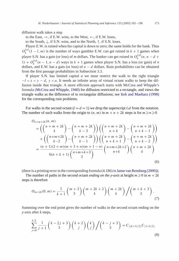
For walks in the second octant (l= d = 1) we drop the superscriptl|/d from the notation.The number of such walks from the origin to(n,m) in m+ n+ 2k steps is form�n�0
On+m+2k(n,m)
=((
n+m+ 2kk
)−(n+m+ 2k
k − 3))((
n+m+ 2kn+ k
)−(n+m+ 2kn+ k − 1
))
+((
n+m+2kk−2
)−(n+m+ 2k
k − 1))((
n+m+ 2kn+ k + 1
)−(n+m+ 2kn+ k − 2
))
= (n+ 1)(2+m)(m+ 3+ n)(m+ 1− n)
6(n+ k + 1)(n+m+k+3
3
) (n+m+2k+2
n+k)(
n+m+ 2kk
)
(6)
(there is a printing error in the corresponding formula (4.186) inJanse vanRensburg (2000)).The number of paths in the second octantending on the y-axisat heightm�0 inm+ 2k
steps is therefore
Om+2k(0,m)= 1
k + 1(m+ 33
)(m+ 2k + 2
k
)(m+ 2k
k
)/(m+ k + 3
3
).
(7)
Summing over the end point gives the number of walks in the second octant ending on they-axis afterk steps,
k/2∑j=0
1
j + 1(k − 2j + 3
3
)(k + 2j
)(k
j
)/(k − j + 3
3
)= C (k+1)/2�C 1+k/2�
(8)
174 H. Niederhausen / Journal of Statistical Planning and Inference 135 (2005) 165–196
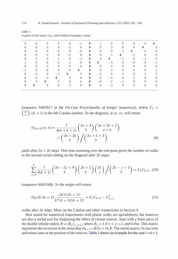
Table 1A piece of the matrixO4, with boldface boundary values
0 0 0 0 0 −1 0 1 0 0 0 0 00 0 0 0 −3 0 0 0 3 0 0 0 00 0 0 −2 0 −6 0 6 0 2 0 0 00 0 2 0 −5 0 0 0 5 0 −2 0 00 3 0 5 0 −3 0 3 0 −5 0 −3 01 0 6 0 3 0 0 0 −3 0 −6 0 −10 0 0 0 0 0 0 0 0 0 0 0 0−1 0 −6 0 −3 0 0 0 3 0 6 0 10 −3 0 −5 0 3 0 −3 0 5 0 3 00 0 −2 0 5 0 0 0 −5 0 2 0 00 0 0 2 0 6 0 −6 0 −2 0 0 00 0 0 0 3 0 0 0 −3 0 0 0 0
(sequence A005817 in theOn-Line Encyclopedia of Integer Sequences), whereCk =(2kk
)/(k + 1) is thekth Catalan number. To the diagonal, at(n, n), will return
O2n+2k(n, n)= 1
4(n+ k + 1)(2n+ 43
)(2n+ 2k + 2
n+ k
)
×(2n+ 2k
k
)/(2n+ k + 3
3
)(9)
paths after 2n+ 2k steps. This time summing over the end point gives the number of walksin the second octant ending on the diagonal after 2k steps,
k∑j=0
1
4(k + 1)(2k − 2j + 4
3
)(2k + 2
k
)(2kj
)/(2k − j + 3
3
)= CkCk+1 (10)
(sequence A005568). To the origin will return
O2k(0,0)= 12 (2k)!(2k + 1)!k!2(k + 3)!(k + 2)! = CkCk+2− C2k+1 (11)
walks after 2k steps. More on the Catalan and other connections in Section 4.Best suited for numerical experiments with planar walks are spreadsheets, but matrices
are also a useful tool for displaying the effect of virtual sources. Start with a finite piece ofthe double infinitematrixR=(Rij )i,j∈Z, whereRij=1 if |i+j |=1, and 0 else. Thismatrixrepresents the recursion in the sense thatOk+1=ROk+OkR. The initialmatrixO0 has onesandminus ones at the position of the sources.Table 1showsanexample for the casel=d=1.
H. Niederhausen / Journal of Statistical Planning and Inference 135 (2005) 165–196 175
2.3.1. Three-dimensional diffusionThe samecancellation principle canbeapplied to solve 3-Ddiffusion problems.However,
it is much harder to place the sources in space just by geometrical intuition. For example,consider the 3-D diagonal diffusion with eight step vectors(±1,±1,±1), and require thatthe walks (weakly) stay in the conez�y�x�0. Denote byDk(n,m, l) the number ofwalks from the origin to(n,m, l) in k steps. Ifn,m, l, andk are not of the same parity, thisnumber will be zero. Thus the bounding planes to be avoided by the walk are of the formx = −1, y = x − 2, andz = y − 2. We derive the location of the sources by an algebraicinstead of a visual argument.Let S be the set of sources. If(a, b, c) is a source, then its effect on the boundaries
x=−1,y= x−2, andz= y−2 must be canceled by the opposite sources atf (a, b, c) :=(−a − 2, b, c), g(a, b, c) := (b + 2, a − 2, c), andh(a, b, c) := (a, c + 2, b − 2), re-spectively. Denote byC the noncommutative group generated by the three reflectionsf,g, andh. Hence(a, b, c) ∈ S implies p(a, b, c) ∈ S for all p ∈ C. In other words,S = {p(0,0,0) : p ∈ C}. For a better understanding ofSandCwe temporarily move theorigin into the intersection of the three planes, so that(0,0,0) �→ (1,3,5). The three re-flections are nowf ′(a, b, c)= (−a, b, c), g′(a, b, c)= (b, a, c), andh′(a, b, c)= (a, c, b).Correspondingly,C′ is the group generated byf ′,g′ andh′, andS′={p′(1,3,5) : p′ ∈ C′}.Note thatg′ andh′ are transpositions on three elements. In cycle notation,g′ = (a, b), (c)
andh′ = (a), (b, c). The third transposition can be obtained ash′g′h′ = (a, c)(b). Henceg′ andh′ generate the group of all 3-permutations,S3, which implies that any permuta-tion of (1,3,5) is in S′. The reflectionf ′ changes the sign of the first coordinate,g′f ′g′the sign of the second, andh′g′f ′g′h′ the sign of the third. Hence the 48 elements ofS′are the permutations of(±1,±3,±5).The groupC′ is well-known as the group gener-ated by the symmetries of the cube (the hyperoctahedral group on signed 3-permutations).Every elementp′ of C′ can be written as a composition of transpositions (g′, h′, h′g′h′)and some sign changes induced byf ′. The parity of the number of transpositions inp′is an invariant, and so is the parity of the number of sign changesf ′. We callp′ evenor odd depending on the parity of the number of transpositions plus sign changes. Aneven (odd)p′ can only be written as a composition of an even (odd) number of reflec-tions. Now we return to our set of sources,S = {p′(1,3,5) − (1,3,5) : p′ ∈ C′}. Asources = p′(1,3,5) − (1,3,5) is positive iff p′ is even. We have shown the followinglemma.
Lemma 2. LetP := {(±u,±v,±w), where(u, v,w) is a permutation of(1,3,5)}. Then{(−1,−3,−5)+(x, y, z) : (x, y, z) ∈ P } is the set of sources. The sources(−1,−3,−5)+(x, y, z) and(−1,−3,−5) + ((−1)ix, (−1)j y, (−1)kz) have the same sign iffi + j + k
is even.
The 3-D version ofFig. 4 would show that unrestricted diagonal diffusion in threedimensions is generated by three independent random walks along the three coordinateaxis. The number of unrestricted walks to(n,m, l) in k steps is thereforeUk(n,m, l) :=(
k(k+n)/2
) (k
(k+m)/2) (
k(k+l)/2). After adding up the 48 unrestricted walks starting at the 48
sources inSwith the appropriate signs we arrive atDk(n,m, l). It follows from the above
176 H. Niederhausen / Journal of Statistical Planning and Inference 135 (2005) 165–196
Fig. 4. Diagonal diffusion generated by two perpendicular integer walks. The subscripts and superscripts indicatethe position at stepk of the vertical and horizontal walks, respectively (see Subsection 4.1).
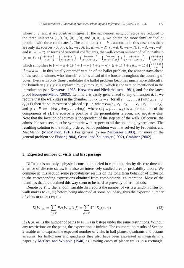
Lemma that
Dk(n,m, l)
=7∑
i=0(−1) i/4�+ i/2�+i
×
∣∣∣∣∣∣∣∣∣∣∣∣∣∣
(k
k + n+ 1− (−1) i/4�2
) (k
k + n+ 1− 3(−1) i/2�2
) (k
k + n+ 1− 5(−1)i2
)(
kk +m+ 3− (−1) i/4�
2
) (k
k +m+ 3− 3(−1) i/2�2
) (k
k +m+ 3− 5(−1)i2
)(
kk + l + 5− (−1) i/4�
2
) (k
k + l + 5− 3(−1) i/2�2
) (k
k + l + 5− 5(−1)i2
)
∣∣∣∣∣∣∣∣∣∣∣∣∣∣.
To shorten the expansion, we defineBit :=(
k(k+i)/2)−(
kt+(k+i)/2
)and find
Dk(n,m, l)= Bn1(B
m3 B
l5− Bm−2
5 Bl+23 )+ Bm+2
1 (Bn−45 Bl+2
3 − Bn−23 Bl
5)
+ Bl+41 (Bn−2
3 Bm−25 − Bn−4
5 Bm3 ). (12)
The special caseD2k(0,0,0) gives formula (1).We chose the example of an eight-step diagonal diffusion in view of an application to
counting watermelons at the end of Section 4.1. The more common “nearest neighborwalks” with six steps(±1,0,0), (0,±1,0), and(0,0,±1) can be enumerated in the sameway, with boundariesx = −1, y = x − 1, andz = y − 1, and corresponding sources at(a, b, c)− (1,2,3), where(a, b, c) is a permutation of(±1,±2,±3). The same approachsolves the boundary problem that restricts the walks to the region
x >− b, y >x − c, z> y − d,
H. Niederhausen / Journal of Statistical Planning and Inference 135 (2005) 165–196 177
whereb, c, andd are positive integers. If the six nearest neighbor steps are reduced tothe three unit steps(1,0,0), (0,1,0), and(0,0,1), we obtain the more familiar “ballotproblem with three candidates” . The conditionx >− b is automatic in this case, thus thereare only six sources,(0,0,0), (c,−c,0), (c, d,−c−d), (c+d,0,−c−d), (c+d,−c,−d),and(0, d,−d). In terms of trinomial coefficients, the well-known number of ballot paths to(n,m, l) is
(l+n+mn,m
)−(
l+n+mn−c,m+c
)+(
l+n+mn−c,m−d
)−(
l+n+mn−c−d,m
)+(
l+n+mn−c−d,m+c
)−(l+n+mn,m−d)
which simplifies to[(m− n+ 1)(l+ 1−m)(l+ 2− n)/((l+ 1)(l+ 2)(m+ 1))](l+n+mn,m
)if c= d = 1. In this “totally ordered” version of the ballot problem, the winner stays aheadof the second winner, who himself remains ahead of the looser throughout the counting ofvotes. Even with only three candidates the ballot problem becomes much more difficult ifthe boundaryz�y�x is replaced byz� max(x, y), which is the version mentioned in theintroduction (seeKreweras, 1965; Kreweras and Niederhausen, 1981), and for the latestproof Bousquet-Mélou (2002). Lemma 2 is easily generalized to any dimensiond. If werequire that the walk stays in the chamberxi > xi−1− ci for all i=1, . . . , d (with x−1=0,ci �1), then the sourcesmust beplacedatp−c, wherec=(c1, c1+c2, . . . , c1+c2+· · ·+cd),andp ∈ P := {(±u1,±u2, . . . ,±ud), where(u1, u2, . . . , ud) is a permutation of thecomponents ofc}.The source is positive if the permutation is even, and negative else.Note that the location of sources is independent of the step set of the walk. Of course, theadmissible step sets must be symmetric with respect to all the bounding hyperplanes. Theresulting solution to the totally ordered ballot problem was first solved by Frobenius andMacMahon (MacMahon, 1916). For generalc′i s seeZeilberger (1983). For more on thegeneral problem seeFisher (1984), Gessel and Zeilberger (1992), Grabiner (2002).
3. Expected number of visits and first passage
Diffusion is not only a physical concept, modeled in combinatorics by discrete time anda lattice of discrete states, it is also an intensively studied area of probability theory. Wecompare in this section some probabilistic results on the long term behavior of diffusionto the corresponding expressions obtained from combinatorial enumeration. Most of theidentities that are obtained this way seem to be hard to prove by other methods.Denote byVn,m the random variable that reports the number of visits a random diffusion
walk makes to(n,m) before being absorbed at some boundary, thus the expected numberof visits to(n,m) equals
E[Vn,m] =∑j �0
Pr(Vn,m�j)=∑k�0
4−kDk(n,m) (13)
if Dk(n,m) is the number of paths to(n,m) in k steps under the same restrictions. Withoutany restrictions on the paths, the expectation is infinite. The enumeration results of Section2 enable us to express the expected number of visits in half planes, quadrants and octantsas sums; for half-planes and quadrants they also have been expressed as integrals in apaper byMcCrea and Whipple (1940)as limiting cases of planar walks in a rectangle.
178 H. Niederhausen / Journal of Statistical Planning and Inference 135 (2005) 165–196
However, those integrals look different from the obvious integrals (16) obtained from thecombinatorial sums!
3.1. Half-planes
Denote byEl|H [Vn,m] the expected number of visits to the point(n,m) of a random
diffusion walk in the half-planex > − l. Because of symmetry,El|H [Vn,m] = E
l|H [Vn,−m],
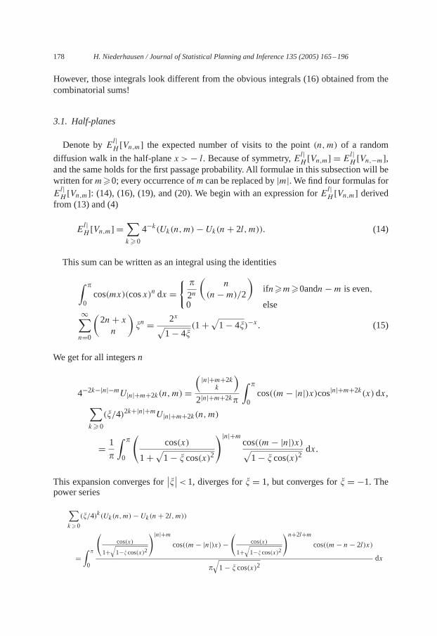
and the same holds for the first passage probability. All formulae in this subsection will bewritten form�0; every occurrence ofmcan be replaced by|m|. We find four formulas forEl|H [Vn,m]: (14), (16), (19), and (20). We begin with an expression forE
l|H [Vn,m] derived
from (13) and (4)
El|H [Vn,m] =
∑k�0
4−k(Uk(n,m)− Uk(n+ 2l, m)). (14)
This sum can be written as an integral using the identities
∫ �
0cos(mx)(cosx)n dx =
{ �2n
(n
(n−m)/2
)ifn�m�0andn−m is even,
0 else∞∑n=0
(2n+ x
n
)�n = 2x√
1− 4� (1+√1− 4�)−x . (15)
We get for all integersn
4−2k−|n|−mU|n|+m+2k(n,m)=( |n|+m+2k
k
)2|n|+m+2k�
∫ �
0cos((m− |n|)x)cos|n|+m+2k(x)dx,∑
k�0(�/4)2k+|n|+mU|n|+m+2k(n,m)
= 1�
∫ �
0
(cos(x)
1+√1− � cos(x)2
)|n|+mcos((m− |n|)x)√1− � cos(x)2
dx.
This expansion converges for∣∣�∣∣<1, diverges for� = 1, but converges for� = −1. The
power series
∑k�0
(�/4)k(Uk(n,m)− Uk(n+ 2l, m))
=∫ �
0
(cos(x)
1+√1−� cos(x)2
)|n|+mcos((m− |n|)x)−
(cos(x)
1+√1−� cos(x)2
)n+2l+mcos((m− n− 2l)x)
�√1− � cos(x)2
dx
H. Niederhausen / Journal of Statistical Planning and Inference 135 (2005) 165–196 179
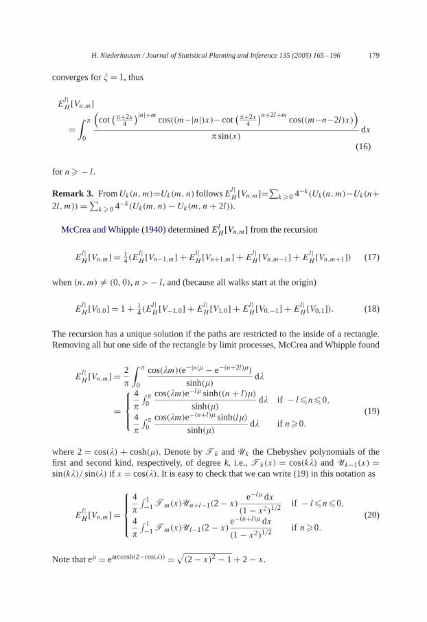
converges for�= 1, thus
El|H [Vn,m]
=∫ �
0
(cot(�+2x4
)|n|+mcos((m−|n|)x)− cot(�+2x4 )n+2l+m cos((m−n−2l)x))
� sin(x)dx
(16)
for n� − l.
Remark 3. FromUk(n,m)=Uk(m, n) followsEl|H [Vn,m]=
∑k�0 4
−k(Uk(n,m)−Uk(n+2l, m))=∑k�0 4
−k(Uk(m, n)− Uk(m, n+ 2l)).
McCrea andWhipple (1940)determinedElH [Vn,m] from the recursion
El|H [Vn,m] = 1
4(El|H [Vn−1,m] + E
l|H [Vn+1,m] + E
l|H [Vn,m−1] + E
l|H [Vn,m+1]) (17)
when(n,m) �= (0,0), n>− l, and (because all walks start at the origin)
El|H [V0,0] = 1+ 1
4(El|H [V−1,0] + E
l|H [V1,0] + E
l|H [V0,−1] + E
l|H [V0,1]). (18)
The recursion has a unique solution if the paths are restricted to the inside of a rectangle.Removing all but one side of the rectangle by limit processes, McCrea andWhipple found
El|H [Vn,m] =
2
�
∫ �
0
cos(�m)(e−|n|� − e−(n+2l)�)sinh(�)
d�
=
4
�
∫ �0cos(�m)e−l� sinh((n+ l)�)
sinh(�)d� if − l�n�0,
4
�
∫ �0cos(�m)e−(n+l)� sinh(l�)
sinh(�)d� if n�0.
(19)
where 2= cos(�) + cosh(�). Denote byTk andUk the Chebyshev polynomials of thefirst and second kind, respectively, of degreek, i.e.,Tk(x) = cos(k�) andUk−1(x) =sin(k�)/ sin(�) if x = cos(�). It is easy to check that we can write (19) in this notation as
El|H [Vn,m] =
4
�
∫ 1−1Tm(x)Un+l−1(2− x)
e−l� dx(1− x2)1/2
if − l�n�0,
4
�
∫ 1−1Tm(x)Ul−1(2− x)
e−(n+l)� dx(1− x2)1/2
if n�0.(20)
Note that e� = earccosh(2−cos(�)) =√(2− x)2− 1+ 2− x.
180 H. Niederhausen / Journal of Statistical Planning and Inference 135 (2005) 165–196
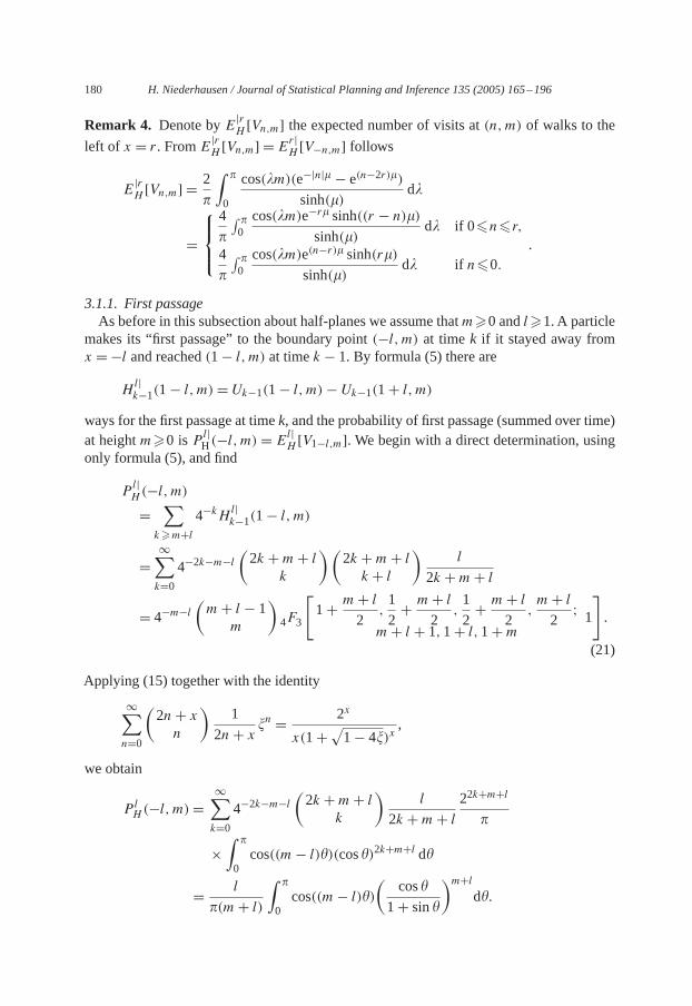
Remark 4. Denote byE|rH [Vn,m] the expected number of visits at(n,m) of walks to theleft of x = r. FromE|rH [Vn,m] = E
r|H [V−n,m] follows
E|rH [Vn,m] =
2
�
∫ �
0
cos(�m)(e−|n|� − e(n−2r)�)sinh(�)
d�
=
4
�
∫ �0cos(�m)e−r� sinh((r − n)�)
sinh(�)d� if 0�n�r,
4
�
∫ �0cos(�m)e(n−r)� sinh(r�)
sinh(�)d� if n�0.
.
3.1.1. First passageAs before in this subsection about half-planes we assume thatm�0 andl�1. A particle
makes its “first passage” to the boundary point(−l, m) at timek if it stayed away fromx =−l and reached(1− l, m) at timek − 1. By formula (5) there are
Hl|k−1(1− l, m)= Uk−1(1− l, m)− Uk−1(1+ l, m)
ways for the first passage at timek, and the probability of first passage (summed over time)at heightm�0 isP l|
H (−l, m) = El|H [V1−l,m]. We begin with a direct determination, using
only formula (5), and find
Pl|H (−l, m)=∑
k�m+l4−kH l|
k−1(1− l, m)
=∞∑k=04−2k−m−l
(2k +m+ l
k
)(2k +m+ l
k + l
)l
2k +m+ l
= 4−m−l(m+ l − 1
m
)4F3
[1+ m+ l
2,1
2+ m+ l
2,1
2+ m+ l
2,m+ l
2;
m+ l + 1,1+ l,1+m1
].
(21)
Applying (15) together with the identity
∞∑n=0
(2n+ x
n
)1
2n+ x�n = 2x
x(1+√1− 4�)x ,we obtain
P lH (−l, m)=
∞∑k=04−2k−m−l
(2k +m+ l
k
)l
2k +m+ l
22k+m+l
�
×∫ �
0cos((m− l)�)(cos�)2k+m+l d�
= l
�(m+ l)
∫ �
0cos((m− l)�)
(cos�1+ sin�
)m+ld�.
H. Niederhausen / Journal of Statistical Planning and Inference 135 (2005) 165–196 181
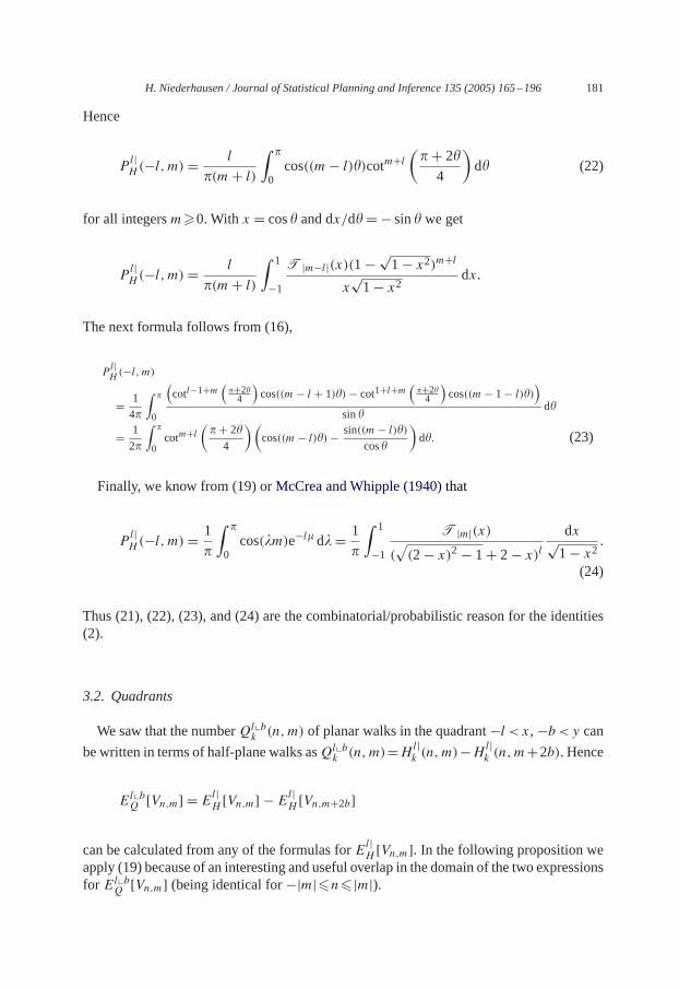
Hence
Pl|H (−l, m)=
l
�(m+ l)
∫ �
0cos((m− l)�)cotm+l
(�+ 2�4
)d� (22)
for all integersm�0. With x = cos� and dx/d�=− sin� we get
Pl|H (−l, m)=
l
�(m+ l)
∫ 1−1
T|m−l|(x)(1−√1− x2)m+l
x√1− x2
dx.
The next formula follows from (16),
Pl|H(−l, m)
= 1
4�
∫ �
0
(cotl−1+m
(�+2�4
)cos((m− l + 1)�)− cot1+l+m
(�+2�4
)cos((m− 1− l)�)
)sin�
d�
= 1
2�
∫ �
0cotm+l
(�+ 2�4
)(cos((m− l)�)− sin((m− l)�)
cos�
)d�. (23)
Finally, we know from (19) orMcCrea andWhipple (1940)that
Pl|H (−l, m)=
1
�
∫ �
0cos(�m)e−l� d�= 1
�
∫ 1−1
T|m|(x)(√(2− x)2− 1+ 2− x)l
dx√1− x2
.
(24)
Thus (21), (22), (23), and (24) are the combinatorial/probabilistic reason for the identities(2).
3.2. Quadrants
We saw that the numberQl�bk (n,m) of planar walks in the quadrant−l < x,−b<y can
be written in terms of half-plane walks asQl�bk (n,m)=Hl|
k (n,m)−Hl|k (n,m+2b). Hence
El�bQ [Vn,m] = E
l|H [Vn,m] − E
l|H [Vn,m+2b]
can be calculated from any of the formulas forEl|H [Vn,m]. In the following proposition we
apply (19) because of an interesting and useful overlap in the domain of the two expressionsfor El�b
Q [Vn,m] (being identical for−|m|�n� |m|).
182 H. Niederhausen / Journal of Statistical Planning and Inference 135 (2005) 165–196
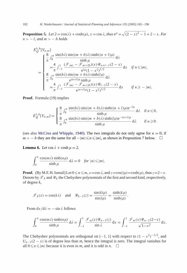
Proposition 5. Let2= cos(�)+ cosh(�), x= cos�, thuse�=√(2− x)2− 1+2− x. For
n>− l, andm>− b holds
El�bQ [Vn,m]
=
8
�
∫ �0sin(b�) sin((m+ b)�) sinh((n+ l)�)
sinh�d�
=4�
∫ 1−1
(T|m| −Tm+2b)(x)Un+l−1(2− x)
el�(1− x2)1/2dx if n� |m|,
8
�
∫ �0sin(b�) sin((m+ b)�) sinh(l�)
e(n+l)� sinh�d�
=4�
∫ 1−1
(T|m| −Tm+2b)(x)Ul−1(2− x)
e(n+l)�(1− x2)1/2dx if n� − |m|.
Proof. Formula (19) implies
El�bQ [Vn,m] =
8
�
∫ �0sin(b�) sin((m+ b)�) sinh((n+ l)�)e−l�
sinh�d� if n�0,
8
�
∫ �0sin(b�) sin((m+ b)�) sinh(l�)e−(n+l)�
sinh�d� if n�0.
(see alsoMcCrea and Whipple, 1940). The two integrals do not only agree forn = 0; ifm>− b they are the same for all−|m|�n� |m|, as shown in Proposition 7 below.�
Lemma 6. Letcos�+ cosh�= 2.∫ �
0
cos(m�) sinh(n�)sinh�
d�= 0 for |n|� |m|.
Proof. (ByM.E.H. Ismail) Let 0�n�m,x=cos�, andz=cos(i�)=cosh(�), thusz=2−x.Denote byTk andUk theChebyshev polynomials of the first and second kind, respectively,of degreek,
Tk(x)= cos(k�) and Uk−1(z)= sin(ki�)sin(i�)
= sinh(k�)sinh(�)
.
From dx/d�=− sin� follows∫ �
0
cos(m�) sinh(n�)sinh�
d�=∫ 1−1
Tm(x)Un−1(z)sin�
dx =∫ 1−1
Tm(x)Un−1(2−x)√1−x2 dx.
The Chebyshev polynomials are orthogonal on[−1,1] with respect to(1− x2)−1/2, andUn−1(2− x) is of degree less thanm, hence the integral is zero. The integral vanishes forall 0�n� |m| because it is even inm, and it is odd inn. �

H. Niederhausen / Journal of Statistical Planning and Inference 135 (2005) 165–196 183
Proposition 7. For max{−|m|,−|m+ 2b|}�n� min{|m|, |m+ 2b|}∫ �
0
sin(�b) sin(�(m+ b)) sinh((n+ l)�)e−l�
sinh�d�
=∫ �
0
sin(�b) sin(�(m+ b)) sinh(l�)e−(n+l)�
sinh�d�.
Proof. From−|m|�n� |m| follows∫ �0 (cos(m�) sinh(n�)/ sinh�)d�=0, and in the sameway∫ �0 (cos(|m+ 2b|�) sinh(n�)/ sinh�)d�= 0. Hence
0=∫ �
0
(cos(m�)− cos((m+ 2b)�)) sinh(n�)sinh�
d�
= 2∫ �
0
sin(�b) sin(�(m+ b)) sinh(n�)sinh�
d�
and∫ �0 (sin(�b) sin(�(m+ b))en�/ sinh�)d�=
∫ �0 (sin(�b) sin(�(m+ b))e−n�/ sinh�)d�.
Subtract∫ �0 (sin(�b) sin(�(m+ b))e−(n+2l)�/ sinh�)d� from both sides and get
∫ �
0
sin(�b) sin(�(m+ b))(en� − e−(n+2l)�)sinh�
d�
=∫ �
0
sin(�b) sin(�(m+ b))(e−n� − e−(n+2l)�)sinh�
d�. �
3.2.1. First passageThe first passage probabilityP l�b
Q (−l, m) to the boundaryx = −l at heightm> − b
equals
Pl|H (−l, m)− P
l|H (−l, m+ 2b)
= 1
2�
∫ �
0
(cotl+|m|
(�+ 2�4
)(cos((|m| − l)�)− sin((|m| − l)�)
cos�
)(25)
−cotl+m+2b(
�+ 2�4
)(cos((m+ 2b − l)�)− sin((m+ 2b − l)�)
cos�
))d�
= 2�
∫ �
0sin(�b) sin(�(m+ b))(2− cos�−
√(2− cos�)2− 1)l d� (26)
= l
�
∫ �
0
cos((|m| − l)�)(
1+ sin�cos�
)|m|+l(|m| + l)
− cos((m+ 2b − l)�)(1+ sin�cos�
)m+2b+l(m+ 2b + l)
d�,(27)
184 H. Niederhausen / Journal of Statistical Planning and Inference 135 (2005) 165–196
using (23), (24), and (22) (remember that cot(� + 2�/4) = cos�/1 + sin�). Note thatP l�bQ (n,−b)= Pb�l
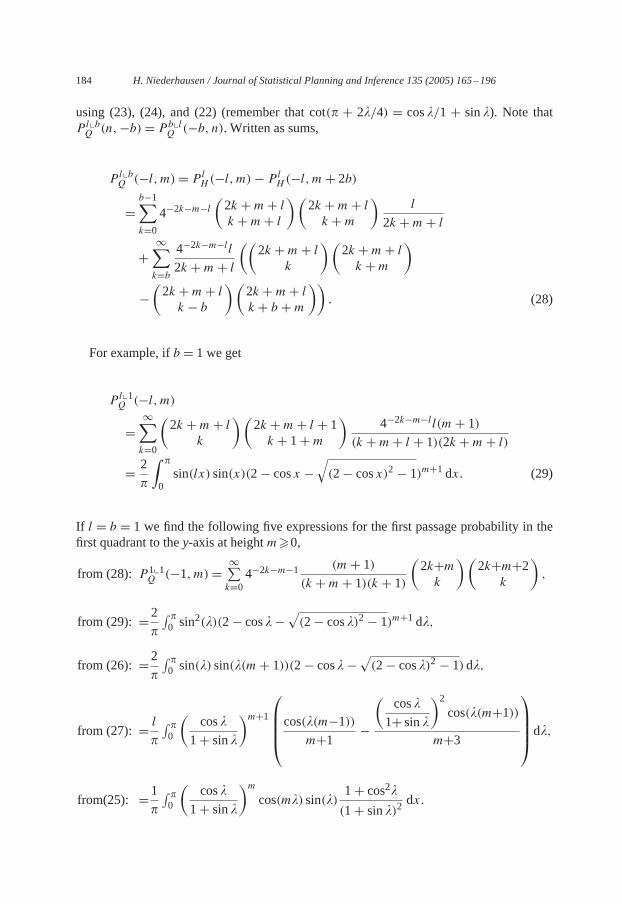
Q (−b, n). Written as sums,
P l�bQ (−l, m)= P l
H (−l, m)− P lH (−l, m+ 2b)
=b−1∑k=04−2k−m−l
(2k +m+ l
k +m+ l
)(2k +m+ l
k +m
)l
2k +m+ l
+∞∑k=b
4−2k−m−l l2k +m+ l
((2k +m+ l
k
)(2k +m+ l
k +m
)
−(2k +m+ l
k − b
)(2k +m+ l
k + b +m
)). (28)
For example, ifb = 1 we get
P l�1Q (−l, m)
=∞∑k=0
(2k +m+ l
k
)(2k +m+ l + 1k + 1+m
)4−2k−m−l l(m+ 1)
(k +m+ l + 1)(2k +m+ l)
= 2�
∫ �
0sin(lx) sin(x)(2− cosx −
√(2− cosx)2− 1)m+1 dx. (29)
If l = b = 1 we find the following five expressions for the first passage probability in thefirst quadrant to they-axis at heightm�0,
from (28): P 1�1Q (−1,m)=∞∑k=04−2k−m−1 (m+ 1)
(k +m+ 1)(k + 1)(2k+mk
)(2k+m+2
k
),
from (29): =2�
∫ �0 sin
2(�)(2− cos�−√(2− cos�)2− 1)m+1 d�,
from (26): =2�
∫ �0 sin(�) sin(�(m+ 1))(2− cos�−
√(2− cos�)2− 1)d�,
from (27): = l
�
∫ �0
(cos�1+ sin�
)m+1cos(�(m−1))m+1 −
(cos�1+ sin�
)2cos(�(m+1))
m+3
d�,
from(25): =1�
∫ �0
(cos�1+ sin�
)mcos(m�) sin(�)
1+ cos2�(1+ sin�)2 dx.
H. Niederhausen / Journal of Statistical Planning and Inference 135 (2005) 165–196 185
3.3. Shifted octants
The numberOl|/dk (n,m) of planar walks in the shifted octant−l < x, y >x − d can be
written in terms of quadrant walks asOl|/dk (n,m) = Ql�l+d
k (n,m) − Ql+d�lk (n − d,m +
d)=Ql�l+dk (n,m)−Ql�l+d
k (m+ d, n− d). Hence
El|/dO [Vn,m] = El�l+d
Q [Vn,m] − El+d�lQ [Vn−d,m+d ]
=El�l+dQ [Vn,m] − El�l+d
Q [Vm+d,n−d ] (30)
for−l−d <n−d <m.We can calculate the probabilityP l|/dO (−l, m) of first passage to the
line x =−l from the first passage probabilities in shifted quadrants. This is not the case forthe first passage to the diagonal liney = x − d, thus we need to knowEl|/d
O [Vn,m]. Formula(30) shows that any of the expressions forEl�b
Q [Vn,m] can be used to findEl|/dO [Vn,m]. An
example is worked out in the following proposition.
Proposition 8. Letcos�+ cosh�= 2, x = cos�, thuse� =√(2− x)2− 1+ 2− x. For
−l − d <n− d <m holds
El|/dO [Vn,m]
={ 8
�
∫ �0
(sin(�(l+d))−sin(�l)e−d�) sin(�(m+l+d)) sinh((n+l)�)el� sinh� d� if n� |m|,
8�
∫ �0sin(�(m+l+d))(sin(�(l+d)) sinh(l�)e−n�−sin(�l) sinh((n+l)�)e−d�)
el� sinh� d� if n� − |m|,
=
4�
∫ 1−1((T|m|−Tm+2(l+d))(x)
el�− (T|m+d|−Tm+d+2l )(x)
e(l+d)�)
if n� |m|,×Un+l−1(2−x)
(1−x2)1/2 dx
4�
∫ 1−1((T|m|−Tm+2(l+d))Ul−1(2−x)
e(n+l)� if n� − |m|.− (T|m+d|−Tm+d+2l )(x)Un+l−1(2−x)
e(l+d)�)
dx√1−x2
Theproof isastraight forwardapplicationofProposition5 toEl|/dO [Vn,m]=El�l+d
Q [Vn,m]−El+d�lQ [Vn−d,m+d ], noting thatn−d� |m+d| inside the shifted octant−l−d <n−d <m.
A different looking formula forEl|/dO [Vn,m] can be derived in the same way if we write
El|/dO [Vn,m] = El�l+d
Q [Vn,m] − El�l+dQ [Vm+d,n−d ].
3.3.1. First passage tox =−lThe probabilityP l|/d
O (−l, m) of first passage strictly inside the shifted octantx > − l,y >x − d to the vertical boundaryx = −l can be obtained in different variations from(25)–(28) because
Pl|/dO (−l, m)= 1
4El|/dO [V1−l,m] = P l�l+d
Q (−l, m)− P l+d�lQ (−l − d,m+ d).
186 H. Niederhausen / Journal of Statistical Planning and Inference 135 (2005) 165–196
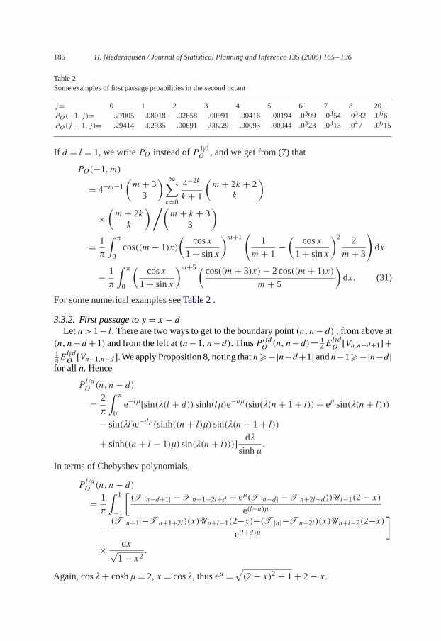
Table 2Some examples of first passage proabilities in the second octant
j= 0 1 2 3 4 5 6 7 8 20PO(−1, j)= .27005 .08018 .02658 .00991 .00416 .00194.0399 .0354 .0332 .066PO(j + 1, j)= .29414 .02935 .00691 .00229 .00093 .00044.0323 .0313 .047 .0615
If d = l = 1, we writePO instead ofP 1|/1O , and we get from (7) that
PO(−1,m)= 4−m−1
(m+ 33
) ∞∑k=0
4−2k
k + 1(m+ 2k + 2
k
)
×(m+ 2k
k
)/(m+ k + 3
3
)
= 1�
∫ �
0cos((m− 1)x)
(cosx
1+ sinx)m+1( 1
m+ 1 −(cosx
1+ sinx)2 2
m+ 3
)dx
− 1�
∫ �
0
(cosx
1+ sinx)m+5(cos((m+ 3)x)− 2 cos((m+ 1)x)
m+ 5)dx. (31)
For some numerical examples seeTable 2.
3.3.2. First passage toy = x − d
Let n>1− l. There are two ways to get to the boundary point(n, n− d) , from above at(n, n−d+1) and from the left at(n−1, n−d). ThusP l|/d
O (n, n−d)= 14El|/dO [Vn,n−d+1]+
14E
l|/dO [Vn−1,n−d ].We apply Proposition 8, noting thatn�−|n−d+1| andn−1�−|n−d|
for all n. Hence
Pl|/dO (n, n− d)
= 2�
∫ �
0e−l�[sin(�(l + d)) sinh(l�)e−n�(sin(�(n+ 1+ l))+ e� sin(�(n+ l)))
− sin(�l)e−d�(sinh((n+ l)�) sin(�(n+ 1+ l))
+ sinh((n+ l − 1)�) sin(�(n+ l)))] d�sinh�
.
In terms of Chebyshev polynomials,
Pl|/dO (n, n− d)
= 1�
∫ 1−1
[(T|n−d+1| −Tn+1+2l+d + e�(T|n−d| −Tn+2l+d))Ul−1(2− x)
e(l+n)�
− (T|n+1|−Tn+1+2l )(x)Un+l−1(2−x)+(T|n|−Tn+2l )(x)Un+l−2(2−x)e(l+d)�
]
× dx√1− x2
.
Again, cos�+ cosh�= 2, x = cos�, thus e� =√(2− x)2− 1+ 2− x.
H. Niederhausen / Journal of Statistical Planning and Inference 135 (2005) 165–196 187
Forn=1− l, the boundary point(1− l,1− l− d) below the corner of the shifted octantcan only be reached from above. HenceP l|/d
O (1− l,1− l − d) = 14E
l|/dO [V1−l,2−l−d ] =
Pl|/dO (−l,2− l − d), the probability of passage to the vertical boundaryx =−l.If the walk is restricted to the second octant (l = b= 1), first passage below the diagonal
to (n, n− 1) happens with probabilityPO(n, n− 1)=∞∑k=0
(4−2k−2(n−1)−1O2(n−1)+2k(n− 1, n− 1)+ 4−2k−2n−1O2n+2k(n, n))
=∞∑k=0
4−2k−2n(n+ 1)(2n+ 2kn+ k − 1
)(2n+ 2k − 2
k
)
3(n+ k)
(2n+ k + 2
4
)× ((n+ 1)(n(2n+ 1)+ 2k(n+ 1))+ k)
= 2�
∫ �
0e−�[sin(2�)e−n�(sin(�(n+ 2))+ e� sin(�(n+ 1)))
−sin(�)e−�
sinh�(sinh((n+ 1)�) sin(�(n+ 2))+ sinh(n�) sin(�(n+ 1)))
]d�.
(32)
4. Related structures
Certain subsets of the diffusion walks in an octant can be visualized by structures thatmay look quite different. We list non-crossing pairs of Dyck paths, bicolored Motzkinpaths, staircase polygons in the second octant, and{→↑}-paths enumerated by left turns.Of course, other aspects of such structures may not be efficiently represented by diffusionwalks. A thorough discussion of these and other structures and their applications can befound inThe Statistical Mechanics of Interacting Walks, Polygons, Animals and Vesicles,by Janse van Rensburg (2000).
4.1. Pairs of non-crossing Dyck paths
The diagonal diffusion, with step set{↗,↙,↘,↖}, is easily mapped onto the ordinarydiffusion by the matrix12
(11−11
). The matrix maps the diagonal steps↗,↙,↘,↖ onto
↑,↓,→,← (in this order). If we draw two independent random walks with steps±1 onthe integers, a vertical walkValong they-axis (marked by
... in Fig. 4) and a horizontal walkH along thex-axis (· · ·), thenthe diagonal diffusion(•) is the vector sum of the two integerwalks, i.e., ifH andV are at the positions(hk,0) and(0, vk) at timek, then(hk, vk) is theposition of the diagonal diffusion walk (this proves formula (3)).If we restrict the one-dimensional walks to nonnegative integers and require that theith
termvi in the vertical walk is not larger than theith termhi in the horizontal walk (makingthemdependent!), i.e.,hi �vi �0 for all i, then the diagonal diffusion stays in the first octant
188 H. Niederhausen / Journal of Statistical Planning and Inference 135 (2005) 165–196
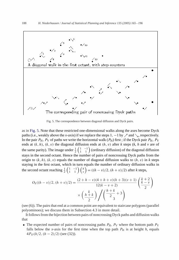
Fig. 5. The correspondence between diagonal diffusion and Dyck pairs.
as inFig. 5. Note that these restricted one-dimensional walks along the axes become Dyckpaths (i.e., weakly above thex-axis) if we replace the steps 1,−1 by↗ and↘, respectively.In the pairPH, PV of paths we write the horizontal walk (PH) first ; if the Dyck pairPH, PVends at(k, h), (k, v) the diagonal diffusion ends at(h, v) afterk steps (k, h andv are of
the same parity). The image under12
(11−11
)(ordinary diffusion) of the diagonal diffusion
stays in the second octant. Hence the number of pairs of noncrossing Dyck paths from theorigin to (k, h), (k, v) equals the number of diagonal diffusion walks to(h, v) in k stepsstaying in the first octant, which in turn equals the number of ordinary diffusion walks in
the second octant reaching12
(11−11
) (hv
)= ((h− v)/2, (h+ v)/2) afterk steps,
Ok((h− v)/2, (h+ v)/2)= (2+ h− v)(4+ h+ v)(h+ 3)(v + 1)12(k − v + 2)
(k + 2k − v
2
)
×(
kh+ k
2
)/( h+ k
2+ 3
3
)
(see (6)). The pairs that end at a common point are equivalent to staircase polygons (parallelpolyominoes); we discuss them in Subsection 4.3 in more detail.It follows from the bijection between pairs of noncrossingDyck paths and diffusionwalks
that
• The expected number of pairs of noncrossing pathsPH, PV where the bottom pathPVfalls below thex-axis for the first time when the top pathPH is at heighth, equals4PO(h/2, (h− 2)/2) (see (32)).
H. Niederhausen / Journal of Statistical Planning and Inference 135 (2005) 165–196 189
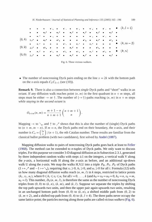
Fig. 6. Three vicious walkers.
• The number of noncrossing Dyck pairs ending on the linex = 2k with the bottom pathon thex-axis equalsCkCk+1 (see (10)).
Remark 9. There is also a connection betweensingleDyck paths and “short” walks in anoctant. If any diffusion walk reaches point(n,m) in the first quadrant inn + m steps, allsteps must be either→ or ↑. The number of{→↑}-paths reaching(n,m) in n + m stepswhile staying in the second octantis
On+m(n,m)= m+ 1− n
n+m+ 1(n+m+ 1
n
).
Mapping→ to↘, and↑ to↗ shows that this is also the number of (single) Dyck pathsto (n + m,m − n). If m = n, the Dyck paths end on their boundary, thex-axis, and their
number isCn=(2nn
)/(n+ 1), thenth Catalan number. These results are familiar from the
classical ballot problem (with two candidates), first solved byAndré (1887).
Mapping diffusion walks to pairs of noncrossing Dyck paths goes back at least toFeller(1968). The method can be extended ton-tuples of Dyck paths. We only want to discusstriples. For this purposeweconsider 3-Ddiagonal diffusionas inSubsection2.3.1, generatedby three independent random walks with steps±1 on the integers, a vertical walk V alongthe y-axis, a horizontal walk H along thex-axis as before, and an additional up-downwalk U along thez-axis. We map the walks H,V,U into a triplePH, PV, PU of Dyck paths(1 �→↗ and−1 �→↘), requiring thatvi �0,hi �0, andui �0 for all i. Formula (12) tellsus how many diagonal diffusion walks reach(n,m, l) in k steps, restricted to lattice points(hi, vi, ui), where 0�hi �vi �ui for all i=0, . . . , k (andh0=v0=u0=0,hk=n, vk=m,uk= l). This number,Dk(n,m, l), is therefore the same as the number of noncrossing Dycktriples from(0,0) to (k, n), (k,m), and(k, l). Suppose we separate the triples by shiftingthe top path upwards two units, and then the upper pair again upwards two units, resultingin an unchanged bottom path from(0,0) to (k, n), a shifted middle path from(0,2) to(k,m+2), and a shifted top path from(0,4) to (k, l+4). The three paths never occupy thesame lattice point; the particlesmoving along those paths are calledvicious walkers(Fig. 6).
190 H. Niederhausen / Journal of Statistical Planning and Inference 135 (2005) 165–196
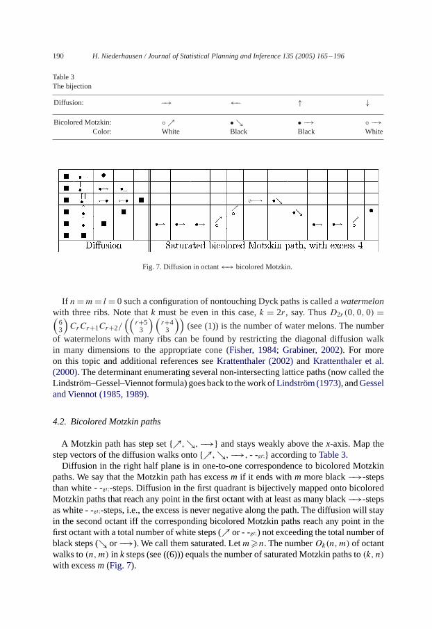
Table 3The bijection
Diffusion: −→ ←− ↑ ↓
Bicolored Motzkin: ◦ ↗ • ↘ • −→ ◦ −→Color: White Black Black White
Fig. 7. Diffusion in octant←→ bicolored Motzkin.
If n=m= l = 0 such a configuration of nontouching Dyck paths is called awatermelonwith three ribs. Note thatk must be even in this case,k = 2r, say. ThusD2r (0,0,0) =(63
)CrCr+1Cr+2/
((r+53
) (r+43
))(see (1)) is the number of water melons. The number
of watermelons with many ribs can be found by restricting the diagonal diffusion walkin many dimensions to the appropriate cone (Fisher, 1984; Grabiner, 2002). For moreon this topic and additional references seeKrattenthaler (2002)andKrattenthaler et al.(2000). The determinant enumerating several non-intersecting lattice paths (now called theLindström–Gessel–Viennot formula) goesback to thework ofLindström (1973), andGesseland Viennot (1985, 1989).
4.2. Bicolored Motzkin paths
A Motzkin path has step set{↗,↘,−→} and stays weakly above thex-axis. Map thestep vectors of the diffusion walks onto{↗,↘,−→, - -gt;} according toTable 3.Diffusion in the right half plane is in one-to-one correspondence to bicolored Motzkin
paths. We say that the Motzkin path has excessm if it ends withmmore black−→-stepsthan white - -gt;-steps. Diffusion in the first quadrant is bijectively mapped onto bicoloredMotzkin paths that reach any point in the first octant with at least as many black−→-stepsas white - -gt;-steps, i.e., the excess is never negative along the path. The diffusion will stayin the second octant iff the corresponding bicolored Motzkin paths reach any point in thefirst octant with a total number of white steps (↗ or - -gt;) not exceeding the total number ofblack steps (↘ or−→). We call them saturated. Letm�n. The numberOk(n,m) of octantwalks to(n,m) in k steps (see ((6))) equals the number of saturated Motzkin paths to(k, n)
with excessm (Fig. 7).
H. Niederhausen / Journal of Statistical Planning and Inference 135 (2005) 165–196 191
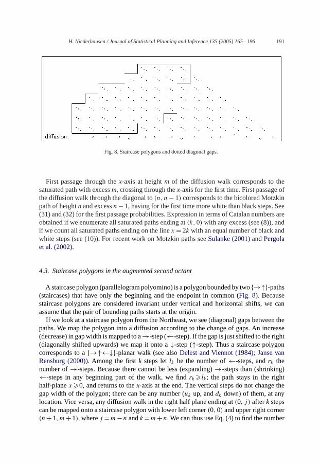
Fig. 8. Staircase polygons and dotted diagonal gaps.
First passage through thex-axis at heightm of the diffusion walk corresponds to thesaturated path with excessm, crossing through thex-axis for the first time. First passage ofthe diffusion walk through the diagonal to(n, n− 1) corresponds to the bicolored Motzkinpath of heightnand excessn−1, having for the first time more white than black steps. See(31) and (32) for the first passage probabilities. Expression in terms of Catalan numbers areobtained if we enumerate all saturated paths ending at(k,0) with any excess (see (8)), andif we count all saturated paths ending on the linex=2k with an equal number of black andwhite steps (see (10)). For recent work on Motzkin paths seeSulanke (2001)andPergolaet al. (2002).
4.3. Staircase polygons in the augmented second octant
Astaircase polygon (parallelogrampolyomino) is a polygon bounded by two{→↑}-paths(staircases) that have only the beginning and the endpoint in common (Fig. 8). Becausestaircase polygons are considered invariant under vertical and horizontal shifts, we canassume that the pair of bounding paths starts at the origin.If we look at a staircase polygon from the Northeast, we see (diagonal) gaps between the
paths. We map the polygon into a diffusion according to the change of gaps. An increase(decrease) in gapwidth ismapped to a→-step (←-step). If the gap is just shifted to the right(diagonally shifted upwards) we map it onto a↓-step (↑-step). Thus a staircase polygoncorresponds to a{→↑←↓}-planar walk (see alsoDelest and Viennot (1984); Janse vanRensburg (2000)). Among the firstk steps letlk be the number of←-steps, andrk thenumber of→-steps. Because there cannot be less (expanding)→-steps than (shrinking)←-steps in any beginning part of the walk, we findrk� lk; the path stays in the righthalf-planex�0, and returns to thex-axis at the end. The vertical steps do not change thegap width of the polygon; there can be any number (uk up, anddk down) of them, at anylocation. Vice versa, any diffusion walk in the right half plane ending at(0, j) afterk stepscan be mapped onto a staircase polygon with lower left corner(0,0) and upper right corner(n+1,m+1), wherej =m−n andk=m+n. We can thus use Eq. (4) to find the number
192 H. Niederhausen / Journal of Statistical Planning and Inference 135 (2005) 165–196
of all staircase polygons from(0,0) to (n,m),
(n+m− 2n− 1
)(n+m− 2m− 1
)−(n+m− 2
m
)(n+m− 1
n
)
a Narayana number. The enumeration by gap width allows for much deeper results than theabove application (seeConway et al. (1997)). A bijection between staircase polygons andbicolored Motzkin paths is described inJanse van Rensburg (2000); for an approach viaskew Ferrer’s diagrams seeDelest and Fedou (1993).We say that a staircase polygon stays in the augmented second octant if it stays weakly
abovey = x − 1. Any staircase polygon is bounded by two{→↑}-paths, starting with alower left corner� at (0,0),and ending with an upper right corner� at (n+ 1,m+ 1), say.If we remove those two corners from a staircase polygon in the augmented second octant,then shift both paths so that they start at the origin and end at(n,m), and turn the shiftedpair downwards by 45◦, we obtain a pair of non-crossing Dyck paths from the origin to thecommon endpoint(n+m,m− n). We enumerated such pairs in Section 4.1; if we denoteby S(n,m) the number of staircase polygons to(n,m) in the augmented second octant, wefind form�n
S(n+ 1,m+ 1)=Om+n(0,m− n)= 6 (m+ n)!(m+ n+ 2)!n!(n+ 1)!(m+ 2)!(m+ 3)!
(m− n+ 3
3
)
(or use formula (7)). Some special cases of staircase polygons in the augmented secondoctant:
• If m= n the polygon ends at(n+ 1, n+ 1), and by (11) there are
6(2n)!(2n+ 2)!
n!(n+ 1)!(n+ 2)!(n+ 3)! = CnCn+2− C2n+1
such staircase polygons.• FromO(n+k)+k(0, n)=S(k+1, n+k+1) follows that the expected number of polygonsendingn vertical steps above the diagonal equals 4PO(−1, n) (see (31)).
• The number of polygons ending on the linen + m = k for given integerk�2 equalsC (k−1)/2�C k/2� (see (8)).
• Thenumber of polygonsendingon thediagonal at(n, n)equalsO2n−2(0,0)=Cn−1Cn+1− C2n (see (11)).
4.4. {→↑}-paths in the augmented third hexadecant enumerated by left turns
Denote by[u, v] the discrete intervalu�x�v, wherex ∈ Z, and by( [u,v]
k
)the set of
all k-element subsets[u, v]. Several interesting combinatorial problems can be bijectivelymapped to
( [u,v]k
)×( [p,q]
l
)(or subsets thereof) for certain choices of the parameters. The
following examples are connected with diffusion walks in the second octant.
H. Niederhausen / Journal of Statistical Planning and Inference 135 (2005) 165–196 193
Lemma 10. Let np, nq and m be nonnegative integers. There exists a bijection between( [0,m+np−1]m
)×( [0,m+nq−1]
m
)and
1. Pairs p, q of {→↑}-paths, starting at the origin and ending at the point(np,m) and(nq,m), respectively.
2. {→↑}-paths, starting at the origin and ending at(m+ np,m+ nq), taking m left turns
( ↑→◦ ).3. {→↑}-paths, starting at the origin and ending at(m+np,m+nq), taking m right turns(◦ →↑ ).
Proof. Consecutively label them + np steps of the pathp with the numbers 0, . . . , m +np − 1. Let xi be the label of theith vertical step, thus 0�x1< · · ·<xm�m + np − 1,and{xi : i ∈ [1,m]} ∈
( [0,m+np−1]m
). In the same way, the labels{yi : i ∈ [1,m]} of the
m vertical steps in the pathq are elements of( [0,m+nq−1]
m
). Vice versa, them-subsets of
[0,m+ np − 1] and[0,m+ nq − 1] correspond to a unique pair of pathsp, q.If we interpret the sequence(xi + 1, yi), i = 1, . . . , m as the sequence of left turn
coordinates we obtain a unique lattice path from the origin to(m + np,m + nq) with mleft turns; vice versa, the left turn sequence of any such path defines a unique element from( [0,m+np−1]
m
)×( [0,m+nq−1]
m
). �
Corollary 11. There exists a bijection between( [0,m+n]
m+1)×( [1,m+n+1]
m+1)
and
1. Pairs of{→↑}-paths,both starting at the origin and ending at the common point(n,m+1).
2. Pairs u, b of {→↑}-paths, both starting at the origin and ending at the common point(n + 1,m + 1) such that u ends and b begins with a horizontal step(in the case ofnonintersecting pairs, u would be the upper and b the bottom path).
3. Diagonal diffusion walks from(0,0) to (n − m − 1, n − m − 1) in n + m + 1 steps,weakly staying inside the rectangle−m− 1�x�n and−m− 1�y�n.
4. {→↑}-paths, starting at the origin and ending at(m+ n+ 1,m+ n+ 1), takingm+ 1right turns(◦ →↑ ).
5. {→↑}-paths, starting at the origin and ending at(m+ n+ 1,m+ n+ 1), takingm+ 1left turns( ↑→ ◦).
Proof. For the terminology we refer to the proof of Lemma 10. Take any pairu′, b′ of{→↑}-paths from the origin to the common endpoint(n,m+ 1). By Lemma 10 such pairscan be bijectively mapped onto
( [0,m+n]m+1)×( [0,m+n]
m+1). Makeb′ into the “bottom” pathb
by inserting a→ step at the beginning ofb, andu′ into theupper pathu by appending a→step at the end ofu (the paths may still intersect; they end at(n+ 1,m+ 1)). The verticallabel subsets are now in
( [0,m+n]m+1)×( [1,m+n+1]
m+1), which shows parts 1 and 2. For part 3,
interpretu′ as the vertical, andb′ as the horizontal walk defining a diagonal diffusion as inFig. 4. The horizontal (vertical) walk movesm+1 steps to the left (downwards) andnsteps
194 H. Niederhausen / Journal of Statistical Planning and Inference 135 (2005) 165–196
to the right (upwards), which defines the boundary for the resulting diagonal diffusion. Parts4 and 5 follow directly from Lemma 10.�
In a staircase polygon to(n + 1,m + 1) the upper and bottom paths make a pairu, b
as in the above bijection, with the additional condition of no common points except at thebeginning and end. Them + 1 positionsxi andyi of the vertical steps in the sequenceof all steps determine the whole pairu, b. Note thatx1 = 0, xm+1�m + n andy1�1,ym+1 = m + n + 1 in every such staircase polygon. Therefore we disregardx1 andym+1,and consider only{xi+1|1� i�m} ∈
([1,m+n]
m
)and{yi |1� i�m} ∈
( [1,m+n]m
). When the
bottom path takes theith vertical step, it has takenyi− i+1 horizontal steps; theith verticalstep leads from the vertex(yi− i+1, i−1) to the vertex(yi− i+1, i), for i=1, . . . , m+1.Exchangex with y and the same holds for the upper pathu. The pairu, b is nontouching;when the bottom pathb moves upwards, to(yi − i + 1, i), it must stay below the upperpath, hencexi+1− (i + 1)+ 1<yi − i + 1, i.e.,
xi+1�yi (33)for all i=1, . . . , m. This condition (together withx1=0 andym+1=m+n+1) characterizesthe staircase polygons. We now map them bijectively onto lattice paths enumerated by leftturns in theaugmented third hexadecant, wherex − 1�y�2x. Instead of creatingm+ 1turns at(xi, yi) as described in the proof of Lemma 10, we place onlym left turns at
(xi+1, yi − 1)i=1,...,m ∈( [1,m+n]
m
)×( [0,m+n−1]
m
), becausex1 andym+1 are fixed in any
staircase polygon. The image path runs from(0,0) to (n+m, n+m) and staysweakly abovey=x−1 because this condition holds at the end point and at all left turns,yi−1�xi+1−1(see (33)).We said in the previous subsection that a staircase polygon to(n + 1,m + 1) is in the
augmented second octant iff the bottom pathb stays weakly abovey = x − 1. To keepbweakly abovey = x − 1 we needi − 1�yi − i, i.e.,yi + 1�2i for i = 1, . . . , m+ 1. Inthe corresponding lattice path the sequence(si, ti) of left turns must satisfy the conditioni�1+ ti/2 for i = 1, . . . , m.The conditioni� ti+1/2 is equivalent to the restriction that every point(v,w) on the path
is reached with at leastw/2 left turns; equivalently, the path stays weakly belowy = 2x.From x − 1�y�2x for all points (x, y) on the path follows that the path stays in theaugmented third hexadecant. Denote byh(v,w; i) the number of{→,↑}-paths from theorigin to (v,w) in the augmented third hexadecant withi left turns. We have shown thath(n+m, n+m;m)=S(n+1,m+1)=Om+n(0,m−n)=6[(m+n)!(m+n+2)!/n!(n+1)!(m+2)!(m+3)!]
(m−n+33
)for allm�n. It is alsoeasy to verify thath(i, 2i; i)=Ci , theith
Catalan number. Fromh(k, k; k−n)=Ok(0, k−2n)and (8) follows thatC (k+1)/2�C 1+k/2�ordinary{→↑}-paths stay in the augmented third hexadecant and end at(k, k) (independentof the number of left turns).
Acknowledgements
This work began with the quest for a simpler proof of a much harder problem, theenumeration of diffusion walks in the second octant, conditioned on the number of visits to
H. Niederhausen / Journal of Statistical Planning and Inference 135 (2005) 165–196 195
thediagonal.1 For ananalytic approach to this question see Janse vanRensburg (2000). I amalso indebted toY. Itoh for drawingmyattention to thepaperbyMcCreaandWhipple (1940),and for the interpretationof diffusion in anoctant asagamblers’ruin problem.M.E.H. Ismailpointed out the connection to Chebyshev polynomials, which helps to “explain” some ofthe identities, and A.J. Guttmann showed me how to enumerate polyominoes by gap size.Finally, most of the references have been provided by one of the referees.
References
André, D., 1887. Solution directe du problème résolu par M. Bertrand. C. R. Acad. Sci. Paris 105, 436–437.Biane, P., 1992. Minuscule weights and random walks on lattices. In: Accardi, L. (Ed.), Quantum Probability &Related Topics. World Scientific Publishing, River Edge, NJ, pp. 51–65.
Bousquet-Mélou, M., 2002. Counting walks in the quarter plane. Trends Math. Birkhäuser, Basel, pp. 49–67.Conway, A., Delest, M., Guttmann, A.J., 1997. The number of three-choice polygons. Math. Comput. Modelling26, 51–58.
Csáki, E., 1997. Some results for two-dimensional random walk. In: Balakrishnan, N. (Ed.), Advances inCombinatorial Methods and Applications to Probability and Statistics. Birkhäuser, Boston, pp. 115–124.
Delest, M.-P., Fedou, J.M., 1993. Enumeration of skew Ferrer’s diagrams. Discrete Math. 112, 65–79.Delest, M., Viennot, G., 1984. Algebraic languages and polyominoes enumeration. Theoret. Comput. Sci. 34, 169–206.
Feller, W., 1968. An Introduction to Probability Theory and its Application. Wiley, NewYork.Fisher, M.E., 1984. Walks, walls, wetting and melting. J. Statist. Phys. 34, 667–729.Gessel, I.M., Viennot, G., 1985. Binomial determinants paths, and hook length formulae. Adv. Math. 58, 300–321.
Gessel, I.M., Viennot, X.G., 1989. Determinants, paths, and plane partitions, preprint, available athttp://www.cs.brandeis.edu/∼ira.
Gessel, I.M., Zeilberger, D., 1992. Random walk in a Weyl chamber. Proc. Amer. Math. Soc. 115, 27–31.Gouyou-Beauchamps, D., 1986. Chemins sous-diagonaux et tableau de Young. in: Combinatoire Enumerative,Lecture Notes in Mathematics, vol. 1234, Montreal, 1985, pp. 112–125.
Grabiner, D.J., 2002. Random walk in an alcove of an affine Weyl group, and noncolliding random walks on aninterval. J. Combin. Theory Ser. A 97, 285–306.
Guy, R.K., Krattenthaler, C., Sagan, B.E., 1992. Lattice paths, reflections, and dimension changing bijections.ArsCombin. 34, 3–15.
Itoh, Y., Maehara, H., 1998. A variation to the ruin problem. Math. Japon. 47, 97–102.Janse van Rensburg, E.J., 2000. The Statistical Mechanics of Interacting Walks, Polygons, Animals and Vesicles.Oxford University Press, Oxford, UK.
Krattenthaler, C., 2002. Watermelon configurations with wall interaction: exact and asymptotic results. J. Statist.Plann. Inference, to appear.
Krattenthaler, C., Guttmann, A.J., Viennot, X.G., 2000. Vicious walkers, friendly walkers andYoung tableaux II:with a wall. J. Phys. A 33, 8835–8866.
Kreweras, G., 1965. Sur une classe de problèmes liés au treillis des partitions d’entiers. Cahiers du B.U.R.O. 6, 5–105.
1 Since the completion of this paper, I have been able to prove by very different andmuch less elegant methods(Niederhausen, 2004) that the number of such walks from the origin to(n, n) in 2k steps makingd contacts withthe diagonal equals(
2k+2k+n+2
) (2kk
)(2k+1d+1)2(k+1)2
((n+1)(d−1)
(k
d−1)+ (2k+1−d)(2n+d+2)
d+1((
k−nd
)−(k
d
)+n(
k
d−1)))
.

196 H. Niederhausen / Journal of Statistical Planning and Inference 135 (2005) 165–196
Kreweras, G., Niederhausen, H., 1981. Solution of an enumerative problem connected with lattice paths. EuropeanJ. Combin. 2, 55–60.
Lindström, B., 1973. On the vector representations of induced matroids. Bull. London Math. Soc. 5, 85–90.McCrea,W.H.,Whipple, F.J.W., 1940. Random paths in two and three dimensions. Proc. Roy. Soc. Edinburgh 60,281–298.
MacMahon, P.A., 1916. Combinatorial Analysis. Reprinted by Chelsea, 1960.Mohanty, S.G., 1979. Lattice Path Counting and Applications. Academic Press, NewYork.Niederhausen, H., 1998. Planar random walks inside a rectangle. Congr. Numer. 132, 125–144.Niederhausen, H., 2002. Planar walks with recursive initial conditions. J. Statist. Plann. Inference 101, 229–253.Niederhausen, H., 2004.A note on the enumeration of diffusionwalks in the first octant by their number of contactswith the diagonal. Electron. J. Integer Sequences, submitted.
Pergola, E., Pinzani, R., Rinaldi, S., Sulanke, R.A., 2002. A bijective approach to the area of generalized Motzkinpaths. Adv. Appl. Math. 28, 580–591.
Sulanke, R.A., 2001. Bijective recurrences for Motzkin paths. Adv. Appl. Math. 27, 627–640.Zeilberger, D., 1983. Andre’s reflection proof generalized to the many-candidate ballot problem. Discrete Math.44, 325–326.