Range Extension Autonomous Driving for Electric Vehicles

IEEJ Transactions on Industry ApplicationsVol.136 No.2 pp.1–8 DOI: 10.1541/ieejias.136.1

Paper

Range Extension Autonomous Driving for Electric VehiclesBased on Optimal Velocity Trajectory Generation and

Front-Rear Driving-Braking Force Distribution

Yuta Ikezawa∗a) Student Member, Hiroshi Fujimoto∗ Senior Member

Yoichi Hori∗ Fellow, Daisuke Kawano∗∗ Non-member

Yuichi Goto∗∗ Non-member, Misaki Tsuchimoto∗∗∗ Non-member

Koji Sato∗∗∗ Non-member

(Manuscript received May 31, 2015, revised December 21, 2015)

Electric vehicles (EVs) have been intensively studied over the past decade, owing to their environmentally-friendlycharacteristics. However, the miles-per-charge of typical EVs is lower than the cruising range of typical internal com-bustion engine vehicles. To increase miles-per-charge, the authors’ research group has proposed a series of controlsystems, including Range Extension Control Systems (RECS) and Range Extension Autonomous Driving (READ)systems. In this paper, by considering the load transfer, slip ratio, motor losses, a READ system is proposed thatoptimizes the velocity trajectory and the front and rear driving-braking force distribution ratio; these techniques helpreduce the consumption energy of the autonomous vehicle. The effectiveness of the proposed method is verified bysimulations and experiments.

Keywords: electric vehicle, driving and braking force distribution, range extension autonomous driving, slip ratio, motor loss

1. Introduction

Due to the increasing concerns on environmental and en-ergy problems, electric vehicles (EVs) have been widelystudied over the past decade. Compared with internal com-bustion engine vehicles (ICEVs), EVs have the following re-markable advantages(1).

( 1 ) Torque generation of a motor is faster than that ofan engine (several milliseconds vs. several hundredmilliseconds).

( 2 ) Motor torque can be estimated precisely from thecurrent.

( 3 ) For EVs with in-wheel motors, each wheel can becontrolled independently.

( 4 ) Motors not only can be used for driving, but alsocan be employed for regenerative braking.

Although EVs have many advantages, they have one prob-lem: the miles-per-charge is relatively short. In order to solvethis problem, many kinds of research have been conducted,and most of studies focused on hardware modifications. Forexample, wireless power transfer for the moving electric ve-hicles, expanding high-efficiency regions of motors, and se-ries chopper power train using a buck-boost chopper(2)∼(4).

a) Correspondence to: [email protected]∗ The University of Tokyo, 5-1-5 Kashiwanoha, Kashiwa, Chiba,

277-8561 Japan∗∗ National Traffic Safety and Environment Laboratory, 7-42-27,

Jindaijihigashimachi, Chofu, Tokyo, 182-0012 Japan∗∗∗ Ono Sokki Co.,Ltd., 3-9-3, Shin-Yokohama, Kohoku-ku, Yoko-

hama, Kanagawa, 222-8507 Japan

On the other hand, the authors’ research group has pro-posed a series of pure control approaches named Range Ex-tension Control Systems (RECS)(5) (6), which do not need tochange the vehicle structures. By utilizing the different motorefficiencies, RECS distributes the total driving-braking forcebetween the front and rear wheels to increase the miles-per-charge. Specifically, several distribution methods are avail-able to minimize the energy loss, for instance, a searchingalgorithm was proposed in (5), and analytically solution wasderived in (6).

Another approach to increase the miles-per-charge is to im-prove traffic flow by using intelligent transport systems (ITS)(7). In (8), a traffic flow management method was studied byplatooning control, and in (9), virtual traffic lights were intro-duced. Along with the development of ITS and autonomousdriving technologies, the vehicle velocity can be designed byconsidering objectives such as energy efficiency, i.e., the con-sumption energy can be reduced by optimizing the velocitytrajectory. There is a article for the minimization of the con-sumption energy of EVs(10), however, important factors suchas the load transfer, slip ratio and motor losses were not takeninto account.

In this paper, by considering the distribution ratio, loadtransfer, slip ratio, motor losses, a Range Extension Au-tonomous Driving (READ) system which minimizes theconsumption energy is proposed for the autonomous vehi-cles. Proposed method optimizes the velocity trajectory anddriving-braking force distribution ration numerically by uti-lizing the vehicle motion and the consumption energy mod-els. In this paper, intervehicular distance information is not

c⃝ 2016 The Institute of Electrical Engineers of Japan. 1

Range Extension Autonomous Driving for EV (Yuta Ikezawaet al.)

considered because we assume that the vehicle runs on thesparse road alone. The effectiveness of the proposed methodis verified by simulations and experiments.

2. Vehicle Model

In this section, the vehicle motion and the inverter in-put power are modeled. The inverter input power model isneeded to modify the control input when optimizing the ve-hicle velocity numerically.

2.1 Vehicle Model In this subsection, a four-wheeldriven vehicle is modeled. As only straight driving is consid-ered, the torques of the right and left motors are equal. Theequations of wheel rotation and vehicle dynamics are givenas

Jω j ω j = T j − rF j , · · · · · · · · · · · · · · · · · · · · · · · · · · · · · · (1)

MV = Fall − sgn(V)FDR(V), · · · · · · · · · · · · · · · · · · · (2)

Fall = 2∑j= f ,r

F j , · · · · · · · · · · · · · · · · · · · · · · · · · · · · · · · (3)

whereJω j is the wheel inertia,ω j is the wheel angular ve-locity, T j is the motor torque,r is the wheel radius,F j is thedriving-braking force of each wheel,M is the vehicle mass,V is the vehicle velocity,FDR is the driving resistance,Fall

is the total driving-braking force, and sgn is a sign function.The subscriptj representsf or r ( f stands for front andrrepresents rear). The driving resistanceFDR is defined as

FDR(V) = µ0Mg + b|V| + 12ρCdAV2, · · · · · · · · · · · · · (4)

whereµ0 is the rolling friction coefficient,b is a factor pro-portional toV, ρ is the air density,Cd is the drag coefficient,andA is the frontal projected area.

Then, the slip ratioλ j is given as

λ j =Vω j − V

max(Vω j ,V, ϵ), · · · · · · · · · · · · · · · · · · · · · · · · · · · · · (5)

whereVω j = rω j is the wheel speed andϵ is a small con-stant to avoid division by zero. It is known that the slip ratioλ is related with the friction coefficientµ as shown in Fig.1 (11). In the region of|λ| << 1, µ is nearly proportional toλ.Define the driving stiffnessDs

′ as the slope of the curve, thedriving-braking force of each wheel is given as

F j = µ jN j ≃ Ds′N jλ j , · · · · · · · · · · · · · · · · · · · · · · · · · · · (6)

whereN j is the normal force of each wheel. When driving atV andFall, Nf andNr are respectively calculated as

Nf (V, Fall) =12

[lrl

Mg −hg

l{Fall − sgn(V)FDR(V)}

], (7)

Nr (V, Fall) =12

[l f

lMg +

hg

l{Fall − sgn(V)FDR(V)}

],(8)

wherel f and lr are respectively the distance from the centerof gravity to front and rear axles,l is the wheelbase, andhg isthe height of the center of gravity.

While driving straight, the required driving-braking forcecan be distributed to each wheel. Since the motors of EVsassumed in this research can be independently controlled, adegree of freedom of the driving-braking force distribution

−1 −0.5 0 0.5 1−1

−0.5

0

0.5

1

Slip ratio [−]

Fri

ctio

n c

oef

fici

ent

[−]

µD

s’λ

Fig. 1. µ-λ Curve.

exists. By introducing front and rear driving-braking forcedistribution ratiok, driving-braking forces can be formulatedbased onFall using the distribution ratiok as follows:

F j =12γ j(k)Fall, · · · · · · · · · · · · · · · · · · · · · · · · · · · · · · (9)

γ j(k) =

1− k ( j = f )

k ( j = r). · · · · · · · · · · · · · · · · · · · · · (10)

The distribution ratiok varies between 0 and 1, wherek = 0means the vehicle is front driven, andk = 1 means the vehicleis rear driven.

2.2 Inverter Input Power Model In this subsection,the inverter input power is modeled. Neglecting the mechan-ical loss of the motor and the inverter loss, the inverter inputpowerPin is described as

Pin = Pout + Pc + Pi , · · · · · · · · · · · · · · · · · · · · · · · · · · · (11)

wherePout is the sum of the mechanical outputs of each mo-tor, Pc is the sum of the copper losses of each motor, andPi

is the sum of the iron losses of each motor(6).Suppose that the torque caused by the wheel inertia and

slip ratioλ j are small enough. Then the motor torqueT j andthe wheel angular velocityω j are given as

T j ≃ rF j , · · · · · · · · · · · · · · · · · · · · · · · · · · · · · · · · · · · · · (12)

ω j ≃Vr

(1+ λ j). · · · · · · · · · · · · · · · · · · · · · · · · · · · · · · · (13)

ThereforePout is calculated as

Pout = 2∑j= f ,r

ω jT j

≃ VFall

∑j= f ,r

(1+

γ j(k)Fall

2Ds′N j(V, Fall)

)γ j(k). · · · · (14)

In the modeling of the copper lossPc, the iron loss resis-tance is neglected for simplicity. Suppose that the magnettorque and theq-axis current are much larger than the reluc-tance torque and thed-axis current, respectively. Then, thesum of the copper lossesPc is given as

Pc = 2∑j= f ,r

Rj iq j2

≃ r2

2Fall

2∑j= f ,r

Rj

Kt j2γ j

2(k), · · · · · · · · · · · · · · · · · · · · · · · (15)

whereRj is the armature winding resistance of the motor,iq j

is theq-axis current, andKt j is the torque coefficient of the

2 IEEJ Trans. IA, Vol.136, No.2, 2016


id iod

icd Rc Ld

ωeLqioq+-

vd

R

(a)d-axis.

iq ioq

icq Rc Lq

ωeLdiod+ -

ωeΨ

R

+

-

vq

(b) q-axis.

Fig. 2. Equivalent circuit of PMSM.

motor.Next, the iron loss is modeled. In this paper, based on the

well-known equivalent circuit model(12). Fig. 2 shows thedandq-axis equivalent circuits of the permanent magnetic syn-chronous motor. From Fig. 2, the sum of the iron lossesPi isexpressed as

Pi = 2∑j= f ,r

vod j2 + voq j

2

Rc j

= 2∑j= f ,r

ωej2

Rc j

{(Ld jiod j + Ψ j

)2+

(Lq jioq j

)2}

≃ 2V2

r2

∑j= f ,r

Pn j2

Rc j

(rLq jγ j(k)Fall

2Kt j

)2

+ Ψ j2

, · · (16)

wherevod j andvoq j are respectively thed andq-axis inducedvoltages,Rc j is the equivalent iron loss resistance,ωej is theelectrical angular velocity of each motor,Ld j is the d-axisinductance,Lq j is theq-axis inductance,iod j and ioq j are re-spectively the differences between thed andq-axis currentsand thed andq-axis components of the iron loss current,Pn j

is the number of pole pairs, andΨ j is the interlinkage mag-netic flux. The equivalent iron loss resistanceRc j is describedas

1Rc j(ωej)

=1

Rc0j+

1Rc1j

′|ωej |. · · · · · · · · · · · · · · · · · · · (17)

In (17), the first and second terms of right hand side are re-spectively the eddy current loss and the hysteresis loss.

3. Range Extension Autonomous Driving

In this section, problem formulation is conducted. In addi-tion, the optimization method of driving-braking force distri-bution ratio is introduced.

3.1 Problem Formulation In this paper, the vehi-cle velocity is assumed to be changed fromV0 to Vf with afixed travel distanceXf −X0. This method minimizes the con-sumption energy betweent0 andtf by optimizing the velocitytrajectory and the front and rear driving-braking force distri-bution ratio. Therefore, the objective function and constraintconditions are expressed as

min.　Win =

∫ tf

t0

Pin(x(t),u(t))dt, · · · · · · · · · · · · (18)

s.t. x = f (x(t),u(t))

=

[1M (Fall − sgn(V)FDR(V))

V

], · · · · · (19)

χ(x(t0)) = x(t0) − x0 =

[V(t0) − V0

X(t0) − X0

]= 0, · · (20)

Table 1. Acceleration time.

Vf [km/h]Acceleration time [s]

Conventional Proposed 1 Proposed 2

30 6.570 6.570 9.10060 13.14 13.14 17.50

ψ(x(tf )) = x(tf ) − xf =

[V(tf ) − Vf

X(tf ) − Xf

]= 0, · · · · (21)

whereWin is the consumption energy,x is the state variable,u is the control variable,x0 is the initial condition, andxf isthe terminal condition. They are defined as

x(t) =

[V(t)X(t)

],u(t) =

[Fall(t)k(t)

]. · · · · · · · · · · · · · · · · · · · (22)

The velocity trajectory and the driving-braking distributionratio minimizing the consumption energy can be calculatedby solving this optimal control problem numerically. In thispaper, steepest descent method is used for optimization.

3.2 Optimization of Driving-Braking Force Distribu-tion Ratio SincePin(k) is a quadratic function ofk, theoptimal distribution ratiokopt which minimizesPin shouldsatisfy∂Pin/∂k|k=kopt = 0. Therefore,kopt is derived as a func-tion of V andFall as

kopt(V, Fall) =

VDs′Nf (V,Fall )

+r2Rf

Kt f2 +

V2

Rc f (ωef )

(Lq f

Ψ f

)2

VDs′∑

j= f ,r

1N j (V,Fall )

+r2∑

j= f ,r

Rj

Kt j2 +V2

∑j= f ,r

1Rc j (ωej )

(Lq j

Ψ j

)2.(23)

By applyingkopt, this problem becomes an one-dimensionalsearch.

4. Simulations

Simulations were conducted to verify the effectiveness ofthe proposed method. In this paper, three velocity trajectorygeneration methods are compared with two conditions whoseterminal conditions are different.

4.1 Comparison Conditions In this section, todemonstrate the effectiveness of the proposed method, simu-lations are conducted with the following two conditions.Condition 1: The initial condition is given asV0 = 0 km/h,t0 = 0 s, the terminal condition is determined asVf = 30km/h, and the travel distance isXf − X0 = 27.38m.Condition 2: The initial condition is given asV0 = 0 km/h,t0 = 0 s, the terminal condition is determined asVf = 60km/h, and the travel distance isXf − X0 = 109.5 m.

In this paper, the following three cases are considered foreach condition. The acceleration time of each case is decidedas Table 1.Conventional: The vehicle velocity changes fromV0 to Vf

at a constant acceleration under the condition thatk = 0.5.Therefore theV(t) andtf are given as

V(t) = V0 +Vf

2 − V02

2(Xf − X0)(t − t0), · · · · · · · · · · · · · · · · (24)

tf =2(Xf − X0)(Vf + V0)

+ t0. · · · · · · · · · · · · · · · · · · · · · · · · (25)

Proposed 1: The velocity trajectory is optimized with thetime constraint for minimal consumption energy. The vehi-cle changes the velocity fromV0 to Vf under the condition



0 2.5 5 7.5 100

10

20

30

Time [s]

Vel

oci

ty V

[km

/h]

Conventional

Proposed 1

Proposed 2

(a) VelocityV.

0 2.5 5 7.5 100

1

2

3

Time [s]

Acc

eler

atio

n a

x [

m/s

2]

Conventional

Proposed 1

Proposed 2

(b) Accelerationax.

0 2.5 5 7.5 100

500

1000

1500

2000

Time [s]

Tota

l dri

vin

g f

orc

e F al

l [N

]

Conventional

Proposed 1

Proposed 2

(c) Total driving dorceFall.

0 2.5 5 7.5 100.2

0.3

0.4

0.5

0.6

Time [s]

Dis

trib

uti

on r

atio

k [

−]

Conventional

Proposed 1

Proposed 2

(d) Distribution ratiok.

0 2.5 5 7.5 100

5

10

15

20

Time [s]

Inver

ter

input

pow

er P

in [

kW

]

Conventional

Proposed 1

Proposed 2

(e) Inverter input powerPin.

0 2.5 5 7.5 100

1

2

3

Time [s]

Co

pp

er l

oss

Pc [

kW

]

Conventional

Proposed 1

Proposed 2

(f) Copper lossPc.

0 2.5 5 7.5 100

0.1

0.2

0.3

0.4

0.5

Time [s]

Iron l

oss

Pi [

kW

]

Conventional

Proposed 1

Proposed 2

(g) Iron lossPi .

Conv. Pro. 1 Pro. 20

5

10

15

20

Tota

l en

ergy l

oss

Wlo

ss[k

Ws]

Wi

Wc

WS

WR

(h) Total energy lossWloss.

Fig. 3. Simulation results 1 (condition 1:Vf = 30km/h, acceleration).

0 5 10 15 200

10

20

30

40

50

60

Time [s]

Vel

oci

ty V

[k

m/h

]

Conventional

Proposed 1

Proposed 2

(a) VelocityV.

0 5 10 15 200

1

2

3

Time [s]

Acc

eler

atio

n a

x [

m/s

2]

Conventional

Proposed 1

Proposed 2

(b) Accelerationax.

0 5 10 15 200

500

1000

1500

2000

2500

Time [s]

Tota

l dri

vin

g f

orc

e F al

l [N

]

Conventional

Proposed 1

Proposed 2

(c) Total driving forceFall.

0 5 10 15 200.2

0.3

0.4

0.5

0.6

Time [s]

Dis

trib

uti

on r

atio

k [

−]

Conventional

Proposed 1

Proposed 2

(d) Distribution ratiok.

0 5 10 15 200

10

20

30

40

50

Time [s]

Inver

ter

input

pow

er P

in [

kW

]

Conventional

Proposed 1

Proposed 2

(e) Inverter input powerPin.

0 5 10 15 200

1

2

3

4

Time [s]

Co

pp

er l

oss

Pc [

kW

]

Conventional

Proposed 1

Proposed 2

(f) Copper lossPc.

0 5 10 15 200

0.5

1

1.5

2

Time [s]

Iron l

oss

Pi [

kW

]

Conventional

Proposed 1

Proposed 2

(g) Iron lossPi .


15

30

45

60

Tota

l en

ergy l

oss

Wlo

ss[k

Ws]

Wi

Wc

WS

WR

(h) Total energy lossWloss.

Fig. 4. Simulation results 2 (condition 2:Vf = 60km/h, acceleration).

thatk = kopt. The terminal timetf is equal to that of the con-ventional method.Proposed 2: The velocity trajectory is optimized withoutconsidering the time constraint for minimal consumption en-ergy. The vehicle velocity changes fromV0 to Vf under thecondition thatk = kopt. The optimal terminal timetfopt isdecided to minimize the consumption energy.

4.2 Simulations Figs. 3 and 4 show the simulationresults. To analyze which loss has great effect on optimiz-ing velocity trajectory,Pout is separated as: the power stored

as the kinetic energy of the vehicle massPM , the sum of thepower stored as the rotational energy of each wheelPJ, theloss caused by the driving resistancePR, and the sum of thelosses caused by the slip of each wheelPS:

Pout = PM + PJ + PR + PS, · · · · · · · · · · · · · · · · · · · · (26)

PM =ddt

(12

MV2

), · · · · · · · · · · · · · · · · · · · · · · · · · · · (27)

PJ = 2∑j= f ,r

ddt

(12

Jω jω j2

), · · · · · · · · · · · · · · · · · · · (28)



PR = FDRV, · · · · · · · · · · · · · · · · · · · · · · · · · · · · · · · · · (29)

PS = FallV∑j= f ,r

λ jγ j(k). · · · · · · · · · · · · · · · · · · · · · · (30)

The integrated values of these values are described as

WX =

∫ tf

t0

PX(x(t),u(t))dt, · · · · · · · · · · · · · · · · · · · · · · (31)

where the subscriptX represents “out”, “M”, “J”, “R”, “S”,“c”, and “i”. WM andWJ can be recovered during decelerat-ing, and they are equal zero in all cases ifV0 = Vf .

To evaluate the real losses,Win can be separated into theenergy that can be recovered during decelerationWkinetic andthe total energy lossWloss:

Wkinetic =WM +WJ, · · · · · · · · · · · · · · · · · · · · · · · · · · · · (32)

Win =Wloss+Wkinetic. · · · · · · · · · · · · · · · · · · · · · · · (33)

Wkinetic is 31.9 kWs in the condition 1,Wkinetic is 128 kWs inthe condition 2.

In the condition 1, the velocity trajectory of the proposedmethod 1 is very similar to that of conventional method asshown in Fig. 3(b). Nevertheless, the total energy loss ofthe proposed method 1 is smaller than that of the conven-tional method. The optimization of the distribution ratiokcontributes to this cutback of the total energy loss.

According to Fig. 4(b), unlike the condition 1, the accel-eration of the proposed method 1 is larger than that of theconventional method att<2.5 s andt>10 s in the condition2. As the velocity becomes higher, the percentage of the cop-per loss to the inverter input power becomes smaller. Largeacceleration att < 2.5 s reduces the required driving force atother speed region. On the other hand, large acceleration att > 10 s shortens the driving time at high speed, and reducesthe energy of the iron loss and the loss caused by the drivingresistance.

Figs. 3(c) and 4(c) show that the proposed method 2 gener-ates smaller driving force at low speed than the conventionalmethod. Therefore the copper loss at low speed becomessmaller than the conventional method as shown in Figs. 3(f)and 4(f). Larger driving force than the conventional methodat high speed shortens the time driving with large iron lossas shown in Figs. 3(g) and 4(g). Therefore the energy of theiron loss becomes smaller than the conventional method.

In the condition 2, terminal timetf is optimized to min-imize the consumption energy. Iftf is smaller thantfopt,the copper loss becomes larger than proposed method 2 be-cause required braking force becomes larger than proposedmethod 2. On the other hand, iftf is larger thantfopt, the losscaused by driving resistance (especially rolling resistance)becomes larger than proposed method 2 because becomeslonger than proposed method 2. Therefore optimal terminaltime is mainly decided by tradeoff between the copper lossand the loss caused by driving resistance.

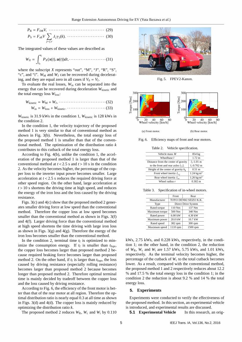
According to Fig. 6, the efficiency of the front motor is bet-ter than that of the rear motor at all region. Therefore the op-timal distribution ratio is nearly equal 0.3 at all time as shownin Figs. 3(d) and 4(d). The copper loss is mainly reduced byoptimizing the distribution ratiok.

The proposed method 2 reducesWR, Wc andWi by 0.110

Fig. 5. FPEV2-Kanon.

Wheel velocity [km/h]

To

rque

[Nm

]

5060

70

75

80

85

90

0 20 40 60 800

100

200

300

(a) Front motor.

Wheel velocity [km/h]

To

rque

[Nm

]

50

60

70

75

80

85

0 20 40 60 800

100

200

300

(b) Rear motor.

Fig. 6. Efficiency maps of front and rear motors.

Table 2. Vehicle specification.

Vehicle massM 854 kgWheelbasel 1.72 m

Distance from the center of gravity l f :1.01 mto the front and rear axlesl f ,lr lr :0.702 m

Height of the center of gravityhg 0.51 mFront wheel inertiaJω f 1.24 kg·m2

Rear wheel inertiaJωr 1.26 kg·m2

Wheel radiusr 0.302 m

Table 3. Specification of in-wheel motors.

Front RearManufacturer TOYO DENKI SEIZO K.K.

Type Direct Drive SystemRated torque 110 Nm 137 Nm

Maximum torque 500 Nm 340 NmRated power 6.00 kW 4.30 kW

Maximum power 20.0 kW 10.7 kWRated speed 382 rpm 300 rpm

Maximum speed 1110 rpm 1500 rpm

kWs, 2.75 kWs, and 0.228 kWs, respectively, in the condi-tion 1; on the other hand, in the condition 2, the reductionof WR, Wc andWi are 1.57 kWs, 5.75 kWs, and 1.01 kWs,respectively. As the terminal velocity becomes higher, thepercentage of the cutback ofWc to the total cutback becomeslower. As a result, compared with the conventional method,the proposed method 1 and 2 respectively reduces about 12.2% and 17.5 % the total energy loss in the condition 1; in thecondition 2 the reduction is about 9.2 % and 14 % the totalenergy loss.

5. Experiments

Experiments were conducted to verify the effectiveness ofthe proposed method. In this section, an experimental vehicleis introduced, and experimental results are discussed.

5.1 Experimental Vehicle In this research, an orig-



CPI

Fall

ax

V V

Ms

rDriving

force

distribution

(1+�j )J�j

r

Fj* Tj

*

Vehicle+ +

+

++

*

*

*

*

k*

Fig. 7. Vehicle speed control system.

inal electric vehicle “FPEV-2 Kanon,” manufactured by theauthors’ research group, is used. Fig. 5 shows the experimen-tal vehicle. This vehicle has four outer-rotor type in-wheelmotors which can be independently controlled. Therefore,driving-braking force distribution among the four wheels ispossible. One of the key factors to design RECS is the differ-ent characteristics of the front and rear in-wheel motors, andFig. 6 shows two motor efficiency maps. Table 2 and 3 showthe specifications of the vehicle and the in-wheel motors, re-spectively.

5.2 Control System Design Fig. 7 shows the veloc-ity control system. The input is the vehicle velocity referenceV∗, and these controllers generate the total driving-brakingforce referenceF∗all. And then,F∗allis distributed to the frontand rear driving-braking force referenceF∗j . Considering theslip ratio, the front and rear torque referenceT∗j is given as

T∗j = rF ∗j +Jω j a

∗x

r(1+ λ∗j ), · · · · · · · · · · · · · · · · · · · · · · (34)

where the second term of the right hand side means the com-pensation of the inertia of the wheels. In this research,λ∗j isgiven as

λ∗j =

0.05 (a∗x > 0)0 (a∗x = 0)−0.05 (a∗x < 0)

. · · · · · · · · · · · · · · · · · · · · (35)

The vehicle velocity controllerCPI is a PI controller, and itis designed by the pole placement method. The plant of thevehicle velocity controller is expressed as

VFall=

1Ms

. · · · · · · · · · · · · · · · · · · · · · · · · · · · · · · · · · · · · (36)

In the simulations and experiments, the poles of the vehiclevelocity controller are set to -5 rad/s.

5.3 Experiments Experiments were conducted sixtimes under respective conditions, using the same conditionsas simulations. In the experiments, we assumed that the vehi-cle velocityV is the average of all the wheel velocities. Theinverter input powerPin was calculated as

Pin = Vdc

∑j= f ,r

Idcj , · · · · · · · · · · · · · · · · · · · · · · · · · · · · · · (37)

whereVdc is the measured input voltage of the inverter andIdcj is the measured input current of the front and rear invert-ers.Pin includes inverter loss.

Figs. 8 and 9 show the experimental results. In Figs. 8(d)and 9(d), error bars represent the standard deviations. Fig.9(b) shows that the total driving-braking force became largerthan that of simulation at high speed region. It means thatthe driving resistance value includes modeling error. FromFigs. 8(d) and 9(d) the results of the total energy loss showthe same tendency as the simulation results. Compared with

the conventional method, the proposed method 1 and 2 re-duced about 13.4 % and 26.9 % the total energy loss in thecondition 1 while the reduction in the condition 2 were about11.0 % and 16.5 % the total energy loss respectively.

6. Conclusion

In this paper, an optimization method named READ wasproposed to minimize the consumption energy. This methodmodels the vehicle motion and the consumption energy,and generates optimal velocity trajectory and driving-brakingforce distribution ratio by solving optimal control problem.Optimal velocity trajectory is mainly decided by tradeoff be-tween the copper loss and the loss caused by driving resis-tance. The effectiveness of the proposed method was veri-fied by simulations and experiments. Specially, the proposedmethod reduced up to 26.9 % total energy loss compared withthe conventional method in the experiments.

However, the proposed method can be applied on straightdriving only. Therefore, an improved algorithm that addressboth driving straight and turning will be studied in the fu-ture. Also, the proposed method can be applied only whena vehicle runs alone. Therefore, it is easy to apply railwaybecause we rarely need to consider another train, however,it is difficult to apply automobiles on the public road. Animproved algorithm that can address on public road even ifthere is another vehicle will be studied. This is achieved byoptimizing the velocities of multiple vehicles simultaneouslyunder intervehicular distance constraint. Another approachis to develop the optimization method having a small calcula-tion load which can update the velocity trajectory consideringintervehicular distance information in real time.

Acknowledgment

This research was partly supported by Industrial Tech-nology Research Grant Program from New Energy and In-dustrial Technology Development Organization (NEDO) ofJapan (number 05A48701d), the Ministry of Education,Culture, Sports, Science and Technology grant (number22246057 and 26249061), and the Core Research for Evo-lutional Science and Technology, Japan Science and Tech-nology Agency (JST-CREST). This result is a part of workin the project team of JST-CREST named “Integrated Designof Local EMSs and their Aggregation Scenario ConsideringEnergy Consumption Behaviors and Cooperative Use of De-centralized In-Vehicle Batteries.”

References

( 1 ) Y. Hori: “Future vehicle driven by electricity and control - research on four-wheel-motored “UOT Electric March II,”” IEEE Trans. on Industrial Elec-tronics, Vol. 51, No. 5, pp. 954–962 (2004).

( 2 ) J. Shin, S. Shin, Y. Kim, S. Ahn, S. Lee,G. Jung, S. J. Jeon, and D. H. Cho:“Design and Implementation of Shaped Magnetic-Resonance-Based Wire-less Power Transfer System for Roadway-Powered Moving Electric Vehi-cles,” IEEE Trans. on Industrial Electronics, Vol. 61, No. 3, pp. 1179–1192(2014).

( 3 ) H. Hijikata and K. Akatsu: “Principle and Basic Characteristic of MATRIXMotor with Variable Parameters Achieved through Arbitrary Winding Con-nections,” IEEJ Journal of Industry Applications, Vol. 2, No. 6, pp. 283–291(2013).

( 4 ) Y. Hosoyamada, M. Takeda, T. Nozaki, N. Motoi, and A. Kawamura: “HighEfficiency Series Chopper Power Train for Electric Vehicles Using a Motor



0 2.5 5 7.5 100

10

20

30

Time [s]

Vel

oci

ty V

[k

m/h

]

Conventional

Proposed 1

Proposed 2

(a) VelocityV.

0 2.5 5 7.5 100

500

1000

1500

2000

Time [s]

To

tal

dri

vin

g f

orc

e F al

l [N

]

Conventional

Proposed 1

Proposed 2

(b) Total driving forceFall.

0 2.5 5 7.5 100

5

10

15

20

Time [s]

Inv

erte

r in

pu

t p

ow

er P

in [

kW

]

Conventional

Proposed 1

Proposed 2

(c) Inverter input powerPin.

Conv.Pro. 1Pro. 20

5

10

15

20

To

tal

ener

gy

lo

ss W

loss

[kW

s]

k=0.5

k=kopt

(d) Total energy lossWloss.

Fig. 8. Experimental results 1 (condition 1:Vf = 30km/h, acceleration).

0 5 10 15 200

10

20

30

40

50

60

Time [s]

Vel

oci

ty V

[km

/h]

Conventional

Proposed 1

Proposed 2

(a) VelocityV.

0 5 10 15 200

500

1000

1500

2000

2500

Time [s]

Tota

l dri

vin

g f

orc

e F al

l [N

]

Conventional

Proposed 1

Proposed 2

(b) Total driving forceFall.

0 5 10 15 200

10

20

30

40

Time [s]

Inver

ter

input

pow

er P

in [

kW

]

Conventional

Proposed 1

Proposed 2

(c) Inverter input powerPin.


15

30

45

60

To

tal

ener

gy l

oss

Wlo

ss[k

Ws]

k=0.5

k=kopt

(d) Total energy lossWloss.

Fig. 9. Experimental results 2 (condition 2:Vf = 60km/h, acceleration).

Test Bench,” IEEJ Journal of Industry Applications, Vol. 4, No. 4, pp. 460–468 (2015).

( 5 ) H. Fujimoto, S. Egami, J. Saito, and K. Handa: “Range Extension ControlSystem for Electric Vehicle Based on Searching Algorithm of Optimal Frontand Rear Driving Force Distribution,” in Proc. 38th Annual Conference ofthe IEEE Industrial Electronics Society, pp. 4244–4249 (2012).

( 6 ) H. Fujimoto and S. Harada: “Model–Based Range Extension Control Systemfor Electric Vehicles With Front and Rear Driving–Braking Force Distribu-tions,” IEEE Trans. on Industrial Electronics, Vol. 62, No. 5, pp. 3245–3254(2015).

( 7 ) J. Zhang, F. Y. Wang, K. Wang, W. H. Lin, X. Xu, and C. Chen: “Data-Driven Intelligent Transportation Systems:A Survey,” IEEE Trans. on Intelli-gent Transportation Systems, Vol. 12, No. 4, pp.1624–1639 (2011).

( 8 ) J. W. Kwon and D. Ghwa: “Adaptive Bidirectional Platoon Control Using aCoupled Sliding Mode Control Method,” IEEE Trans. on Intelligent Trans-port Systems, Vol. 15, No. 5, pp. 2040–2048 (2014).

( 9 ) M. Ferreira and P. M. d’Orey: “On the Impact of Virtual Traffic Lights onCarbon Emissions Mitigation,” IEEE Trans. on Intelligent Transport Systems,Vol. 13, No. 1, pp. 284–295 (2002).

(10) T.Wang and C. G. Cassandras: “Optimal Motion Control for Energy-awareElectric Vehicles,” 2013 IEEE International Conference on Control Applica-tions, pp. 388–393 (2013).

(11) H. B. Pacejka and E. Bakker: “The Magic Formula Tyre Model,” VehicleSystem Dynamics: International Journal of Vehicle Mechanics and Mobility,Vol. 21, No. 1, pp. 1–18 (1992).

(12) S. Morimoto, Y. Tong, Y. Takeda, and T. Hirasa: “Loss Minimization Controlof Permanent Magnet Synchronous Motor Drives,” IEEE Trans. on IndustrialElectronics, Vol. 41, No. 5, pp. 511–517 (1994).

Yuta Ikezawa (Student Member) received the B.S. degree in Depart-ment of Electrical and Electronic Engineering fromThe University of Tokyo, Tokyo, Japan, in 2015. Heis currently working towards the M.S. degree in theDepartment of Advanced Energy, The University ofTokyo, Chiba, Japan. His research interests are opti-mal control systems for electric vehicle. Mr. Ikezawais a student member of IEEE, IEEJ and SAE-Japan.

Hiroshi Fujimoto (Senior Member) received the Ph.D. degree in theDepartment of Electrical Engineering from the Uni-versity of Tokyo in 2001. In 2001, he joined the De-partment of Electrical Engineering, Nagaoka Univer-sity of Technology, Niigata, Japan, as a research asso-ciate. From 2002 to 2003, he was a visiting scholar inthe School of Mechanical Engineering, Purdue Uni-versity, U.S.A. In 2004, he joined the Department ofElectrical and Computer Engineering, Yokohama Na-tional University, Yokohama, Japan, as a lecturer and

he became an associate professor in 2005. He is currently an associate pro-fessor of the University of Tokyo since 2010. He received the Best PaperAward from the IEEE Transactions on Industrial Electronics in 2001 and2013, Isao Takahashi Power Electronics Award in 2010, and Best AuthorPrize of SICE in 2010. His interests are in control engineering, motion con-trol, nano-scale servo systems, electric vehicle control, and motor drive. Dr.Fujimoto is a member of IEEE, the Society of Instrument and Control Engi-neers, the Robotics Society of Japan, and the Society of Automotive Engi-neers of Japan.



Yoichi Hori (Fellow) received his B.S., M.S., and Ph.D. degrees inElectrical Engineering from the University of Tokyo,Tokyo, Japan, in 1978, 1980, and 1983, respectively.In 1983, he joined the Department of Electrical Engi-neering, The University of Tokyo, as a Research As-sociate. He later became an Assistant Professor, anAssociate Professor, and, in 2000, a Professor at thesame university. In 2002, he moved to the Institute ofIndustrial Science as a Professor in the Informationand System Division, and in 2008, to the Department

of Advanced Energy, Graduate School of Frontier Sciences, the Universityof Tokyo. From 1991-1992, he was a Visiting Researcher at the Universityof California at Berkeley. His research fields are control theory and its indus-trial applications to motion control, mechatronics, robotics, electric vehicles,etc. Prof. Hori is the winner of the Best Transactions Paper Award from theIEEE Transactions on Industrial Electronics in 1993, 2001 and 2013, of the2000 Best Transactions Paper Award from the Institute of Electrical Engi-neers of Japan (IEEJ), and 2011 Achievement Award of IEE-Japan. He isan IEEE Fellow and a past AdCom member of IES. He has been the Trea-surer of the IEEE Japan Council and Tokyo Section since 2001. He is alsoa member of the Society of Instrument and Control Engineers; Robotics So-ciety of Japan; Japan Society of Mechanical Engineers; and the Society ofAutomotive Engineers of Japan. He is the past- President of the IndustryApplications Society of the IEEJ, the President of Capacitors Forum, andthe Chairman of Motor Technology Symposium of Japan Management As-sociation (JMA), the Director on Technological Development of SAE-Japan(JSAE) and the Director of Japan Automobile Research Institute (JARI).

Daisuke Kawano (Non-member) received Doctoral degree in the De-partment of Mechanical Engineering from DoshishaUniversity, Japan in 2003. Since February 2003, hehas been affiliated with National Traffic Safety andEnvironment Laboratory, Japan. He works on en-vironmental performance of next-generation vehiclesand alternative fuels.

Yuichi Goto (Non-member) received B.S. and M.S. degrees in the De-partment of Science from Kyoto University, Japanin 1977 and 1979, respectively. He received Ph.Din the Department of Mechanical Engineering fromHokkaido University, Japan in 2002. From 1979 until2001, he has been affiliated with Traffic Safety andNuisance Research Institute (TSNRI) in Ministry ofTransport, Japan. From 2001 until now, he has beenaffiliated with National Traffic Safety and Environ-ment Laboratory (NTSEL) in Ministry of Land, In-

frastructure, Transport and Tourism, Japan. He works as a research coordi-nator of NTSEL.

Misaki Tsuchimoto (Non-member) received a bachelor’s degree inDepartment of engineering and design from ShibauraInstitute of Technology, Japan in 2014. Since April2014, she has been with ONO SOKKI CO., Ltd.She works on the design of a motion control ofautomotive-testing systems.

Koji Sato (Non-member) received B.E. and M.E. degrees in Depart-ment of mechanical and control engineering fromThe University of Electro-Communications, Japan in1992 and 1994, respectively. Since April 1994, hehas been with ONO SOKKI CO., Ltd. He works onthe design of a motion control of automotive-testingsystems.


Documents

Range Extension Autonomous Driving for Electric Vehicles