Embed Size (px)
Citation preview
Tel Aviv UniversityRaymond and Beverly Sackler Faculty of Exact Sciences
Blavatnik School of Computer Science
Range Searching:
Emptiness, Reporting, andApproximate Counting
Thesis submitted for the degree“Doctor of Philosophy”
by
Hayim Shaul
This work was carried out under the supervision of
Professor Micha Sharir
Submitted to the Senate of Tel Aviv University
September 2011

To my wife, Iris, with much love.To my children Noa, Yael and Omer, who taught me the joy of approxi-
mate counting.
Less is more. More’s less.Some is more than emptiness.Count them, more or less.
(Haiku version of this dissertation)
iii

iv
Abstract
In this thesis we study several range searching problems in computational geometry con-centrating on range emptiness problems.
Informally, in a range searching problem we are given a set P of points and are askedto preprocess them into a data structure, such that, given some query range γ of constantdescription complexity, we can quickly count or report the points of P ∩ γ. Emptinesssearching queries, in which we only want to test whether P ∩ γ = ∅, are intuitively easierto answer.
The thesis consists of two major parts. In the first part we discuss several problemsrelated to emptiness searching, involving ray shooting and visibility over terrains. In thesecond part we present a general data structure for answering range emptiness queries withsemialgebraic ranges, and describe several applications of this structure.
Applications of emptiness searching
Ray shooting amid fat triangles in 3-space. Given a set O of n objects, the problemof ray shooting in O is to preprocess O into a data structure such that, given a query rayρ (specified by the point it emanates from, and by its orientation), the first object o ∈ Ohit by ρ can be found efficiently. This problem has received considerable attention due toits application in many geometric problems.
In the most general case, assuming that the objects in O have constant descriptioncomplexity, Agarwal and Matousek [5] showed that with linear storage and near linearpreprocessing, ray shooting in O can be answered in1 O∗(n3/4) time. This is also the bestknown bound for arbitrary triangles. In some special cases better bounds are known. InChapter 2 we consider the case of ray shooting amid fat triangles (where all their anglesare at least some fixed constant), and improve the query time bound to O∗(n2/3).
We also consider a problem where the ray follows a vertical parabolic trajectory, whichwe refer to as stone throwing. Here we consider only the case of stone throwing amidgeneral triangles. Surprisingly, the query time bound for stone throwing is the same as thequery time bound for ray shooting (amid general triangles), namely O∗(n3/4) even thougha vertical parabola has more degrees of freedom than a line.
1The O∗(·) notation hides factors of the form nε, for any ε > 0.
v
Inter-point visibility over terrains in R2 and R
3. Given a set P of n points in R2 or
R3, and a polygonal or polyhedral terrain T with m edges or faces, we say that two points
p1, p2 ∈ P are mutually visible from one another if they lie above T and the segment p1p2
does not intersect T . The visibility graph G is a graph whose vertices are the points of P ,and two vertices are connected by an edge if the points they represent are visible from eachother.
In Chapter 3 we study the problem of determining whether the visibility graph is aclique, i.e., whether every pair of points are visible. We present efficient algorithms forsolving the problem in two and three dimensions, with respective running times O(n log n+m) and O(nm log2 n).
Emptiness searching in semialgebraic settings
The main contribution of this thesis is the extension of Matousek’s emptiness data structurefor half-spaces bounded by hyperplanes [57], to any class of “simply-shaped” semialgebraicranges. Here we seek data structures with linear (or near linear) storage and near linearpreprocessing time, and sub-linear query time, where the goal is to make the query timeas small as possible. This extension is similar to the extension of the range searchingmachinery for half-spaces bounded by hyperplanes [58] to semialgebraic ranges [5], but itfaces additional technical problems, detailed later in the thesis.
Of course one can linearize the given ranges into a higher-dimensional space, i.e., mapthe original points to points lying on on some algebraic surface in higher dimension, assuggested in [5]. However, the query time depends on the dimension of the embeddingspace, and deteriorates as this dimension grows. It is therefore often desirable to constructan emptiness data structure on the points in the original space, in the hope that such astructure yields better performance.
In Chapter 4 we describe our extension of emptiness searching to the semialgebraic case,and apply it to several problems: (i) ray-shooting amid balls in 3-space, with O∗(n2/3) querytime, (ii) finding the farthest point from a convex shape in 3-space with O∗(n1/2) querytime, (iii) finding the closest point to a query point above a query line in the plane, withO∗(1) query time, and (iv) fat-triangle emptiness queries in the plane. For the latterproblem we give a data structure that requires linear storage and answers a query in O∗(1)time, which is comparable with the simple solution that requires O(n log2 n) storage andO(log3 n) query time.
In Chapter 5 we show how to extend the emptiness data structure into an approximatecounting data structure. Here we propose two data structures. The first structure appliesthe technique of Aronov and Har-Peled [15] and uses the emptiness data structure as ablack box. The second data structure is an extension of the data structure of Aronov andSharir [17] to semialgebraic ranges. We also present a solution to the problem of k-heaviestrange searching, where the data points have weights associated with them, and, given aquery range γ and a parameter k, we want to report the k heaviest points in P ∩ γ.
vi

Acknowledgments
First and foremost, I wish to thank my advisor Micha Sharir for his endless guidance andhelp, and especially for his dedication, patience and tolerance.
I would like to thank Sariel Har-Peled, Esther Ezra, Shakhar Smorodinsky for manyhelpful discussions and good advice.
vii

viii
Contents
1 Introduction 11.1 Overview and Background . . . . . . . . . . . . . . . . . . . . . . . . . . . 1
1.1.1 Range searching: overview . . . . . . . . . . . . . . . . . . . . . . . 11.1.2 Multi-level data structures . . . . . . . . . . . . . . . . . . . . . . . 31.1.3 Parametric searching . . . . . . . . . . . . . . . . . . . . . . . . . . 41.1.4 Ray shooting . . . . . . . . . . . . . . . . . . . . . . . . . . . . . . 51.1.5 Cuttings . . . . . . . . . . . . . . . . . . . . . . . . . . . . . . . . . 61.1.6 Shallow ranges . . . . . . . . . . . . . . . . . . . . . . . . . . . . . 71.1.7 Elementary cells . . . . . . . . . . . . . . . . . . . . . . . . . . . . . 81.1.8 Elementary cell partitions . . . . . . . . . . . . . . . . . . . . . . . 81.1.9 (ν, α)-samples and shallow ε-nets. . . . . . . . . . . . . . . . . . . . 10
1.2 Our Results . . . . . . . . . . . . . . . . . . . . . . . . . . . . . . . . . . . 121.2.1 Ray shooting amid fat triangles and stone throwing . . . . . . . . . 121.2.2 Inter-point visibility over terrains in two and three dimensions . . . 131.2.3 Emptiness queries with semialgebraic ranges . . . . . . . . . . . . . 131.2.4 Approximate range counting . . . . . . . . . . . . . . . . . . . . . . 19
2 Ray Shooting and Stone Throwing 212.1 Introduction . . . . . . . . . . . . . . . . . . . . . . . . . . . . . . . . . . . 212.2 Ray Shooting amid Fat Triangles and Other Special Classes . . . . . . . . 22
2.2.1 Preliminaries . . . . . . . . . . . . . . . . . . . . . . . . . . . . . . 222.2.2 Overview of the algorithm . . . . . . . . . . . . . . . . . . . . . . . 222.2.3 Partitioning a triangle into semi-canonical triangles . . . . . . . . . 242.2.4 Finding intersections with semi-canonical curtains . . . . . . . . . . 262.2.5 Determining an intersection with ordinary curtains . . . . . . . . . 282.2.6 Trading space for query time . . . . . . . . . . . . . . . . . . . . . . 29
2.3 Stone Throwing . . . . . . . . . . . . . . . . . . . . . . . . . . . . . . . . . 292.3.1 Testing condition (1.i) . . . . . . . . . . . . . . . . . . . . . . . . . 312.3.2 Testing condition (2.i) . . . . . . . . . . . . . . . . . . . . . . . . . 322.3.3 Shooting along bounded-degree algebraic arcs . . . . . . . . . . . . 33
ix
2.4 Conclusions . . . . . . . . . . . . . . . . . . . . . . . . . . . . . . . . . . . 34
3 Inter-point Visibility over Terrains in Two and Three Dimensions 353.1 Introduction . . . . . . . . . . . . . . . . . . . . . . . . . . . . . . . . . . . 353.2 Terrains in Two Dimensions . . . . . . . . . . . . . . . . . . . . . . . . . . 353.3 Terrains in Three Dimensions . . . . . . . . . . . . . . . . . . . . . . . . . 36
4 Emptiness and Reporting Queries with Semialgebraic Ranges and TheirApplications 414.1 Overview . . . . . . . . . . . . . . . . . . . . . . . . . . . . . . . . . . . . . 414.2 Semialgebraic Range Reporting or Emptiness Searching . . . . . . . . . . . 434.3 Fullness Searching and Reporting Outliers for Convex Ranges . . . . . . . 50
4.3.1 Farthest point from a convex shape . . . . . . . . . . . . . . . . . . 524.3.2 Computing the largest-area, largest-perimeter, and largest-height tri-
angles . . . . . . . . . . . . . . . . . . . . . . . . . . . . . . . . . . 524.4 Ray Shooting Amid Balls in 3-Space . . . . . . . . . . . . . . . . . . . . . 564.5 Range Emptiness Searching and Reporting in the Plane . . . . . . . . . . . 59
4.5.1 Fat triangle reporting and emptiness searching . . . . . . . . . . . . 594.5.2 Range emptiness searching with semidisks and circular caps . . . . 62
4.6 Conclusions . . . . . . . . . . . . . . . . . . . . . . . . . . . . . . . . . . . 67
5 Approximate Semialgebraic Range Counting 695.1 Overview . . . . . . . . . . . . . . . . . . . . . . . . . . . . . . . . . . . . . 695.2 First Approach . . . . . . . . . . . . . . . . . . . . . . . . . . . . . . . . . 705.3 Second Approach . . . . . . . . . . . . . . . . . . . . . . . . . . . . . . . . 71
5.3.1 Choosing the parameters . . . . . . . . . . . . . . . . . . . . . . . . 745.3.2 Analysis of query-time, storage and preprocessing . . . . . . . . . . 745.3.3 Naive implementation . . . . . . . . . . . . . . . . . . . . . . . . . 755.3.4 Solving the recurrences . . . . . . . . . . . . . . . . . . . . . . . . . 785.3.5 Ensuring high probability . . . . . . . . . . . . . . . . . . . . . . . 81
5.4 Reporting the k Heaviest Points in Semialgebraic Ranges . . . . . . . . . . 85
Bibliography 87
x
Chapter 1
Introduction
1.1 Overview and Background
In this thesis we study several problems in computational geometry. Specifically: (i) Wederive improved solutions for ray shooting amid several restricted classes of triangles inthree dimensions, and derive an efficient algorithm for stone throwing (along a parabolictrajectory) amid arbitrary triangles. (ii) We present efficient algorithms for testing forvisibility of all pairs in a given set of points over a polyhedral terrain, in two and threedimensions. (iii) We study the general problems of range emptiness and range reportingwith semialgebraic ranges, and obtain efficient solutions for a wide variety of applications.(iv) Finally, we apply the results in (iii) to obtain efficient data structures for approximaterange counting with semialgebraic ranges.
In this introductory chapter we introduce the needed terminology and notations, reviewearlier works, and describe our results.
1.1.1 Range searching: overview
A range space is a pair (X, Γ), where X is a set and Γ ⊆ 2X is a collection of subsetsof X, called ranges. In our applications, X = R
d, and Γ is a collection of semialgebraicsets of some specific type, each having constant description complexity [69]. That is, eachset in Γ is given as a Boolean combination of a constant number of polynomial equalitiesand inequalities of constant maximum degree. Typical examples of ranges of this kindare half-spaces, balls, cylinders, simplices, hypercubes, etc. To simplify the analysis, weassume1, as in [5], that all the ranges in Γ are defined by a single Boolean combination, sothat each polynomial p in this combination is (d + t)-variate, and each range γ ∈ Γ has tdegrees of freedom, so that if we substitute the values of these t parameters into the lastt variables of each p, the resulting Boolean combination defines the range γ. This allows
1This assumption is not essential, and is only made to simplify the presentation.
2 Introduction
us to represent the ranges of Γ as points in an appropriate t-dimensional parametric space.this assumption holds in practically all of the standard applications.
Under these special assumptions, the range space (X, Γ) has finite VC-dimension, aproperty formally defined in [49]. Informally, it ensures that, for any finite subset P of X,the number of distinct ranges of P , i.e., the number of distinct sets of the form P ∩ γ, forγ ∈ Γ, is O(|P |δ), where δ is (upper bounded by) the VC-dimension.
As a matter of fact, the actual range spaces that we will consider will be of the form(P, ΓP ), where P ⊂ R
d is a finite point set, and each range in ΓP is the intersection ofP with a range in Γ. Given such a range space (P, ΓP ), with |P | = n and with ΓP asthe underlying set of ranges, the range searching problem for (P, ΓP ) is to build a datastructure such that, for a query range γ ∈ Γ, the subset P ∩ γ can be counted, reported,or tested for emptiness efficiently.
In the performance of a range searching data structure, there is usually a trade-offbetween the storage and preprocessing costs on one hand, and the query time on the otherhand. At one end of the spectrum, one seeks a data structure that answers a query in(poly)logarithmic time. In that case the size of the data structure will be polynomial in n,and the goal is to minimize (the exponent in the bound on) the size. At the other end ofthe spectrum, one seeks a linear-size (or near linear-size) data structure. In that case, thequery time will be sub-linear in n, and the goal is to minimize (the exponent in the boundon) the query time. In this thesis we will focus on range searching problems where the sizeof the data structure is linear (or near linear in some cases).
Given a set P ⊂ Rd of n points and a parameter r > 0, Matousek [58] showed how
to build a partition Π of P , of the form Π = (P1, σ1), . . . , (Pm, σm), where, for eachi = 1, . . . ,m, we have n/r ≤ |Pi| ≤ 2n/r, Pi ⊂ P , and σi is a simplex containing Pi,such that each hyperplane crosses at most O(r1−1/d) simplices of Π. Matousek used thismachinery to construct a partition tree for P , where each node v of the tree stores a subsetPv of P , and the children of each internal node v correspond to the subsets of the partitionof Pv. Then, given any range γ which is a half-space bounded by a hyperplane, we cansearch the tree with γ and report P ∩ γ as the disjoint union of O∗(n1−1/d) “canonical”subsets Pv. In particular, this yields a data structure of linear size which supports rangecounting queries on P where the query cost is O∗(n1−1/d). Here, as in the abstract, thenotation O∗(·) hides subpolynomial factors, which are either polylogarithmic of of the formO(nε), for any ε > 0, with a constant of proportionality which depends on ε.
The technique in [58] relies on the linearity of the hyperplanes bounding the rangesand does not work, as is, for more general ranges. For semialgebraic ranges, Agarwal andMatousek [5] showed how to use a lifting scheme to linearize the ranges. For example, if Pis a planar point set and the ranges are disks, then P can be lifted to 3-space by mappingeach point (x, y) to (x, y, x2 + y2). Then a disk, given by (x − x0)
2 + (y − y0)2 ≤ r2, is
mapped to the half-space z ≤ 2x0x + 2y0y + (r2 − x20 − y2
0). See [38] for more details.Hence, querying the original set P with disks is equivalent to querying the lifted set P ∗ by
1.1 Overview and Background 3
half-spaces in R3, which can be done with near-linear storage and O∗(n2/3) query time (for
range counting queries). In general, if the linearization transforms the input set P to a setP ∗ in R
d then one can perform range searching on P (or rather on P ∗) using near-linearstorage and O∗(n1−1/d) query time. Agarwal and Matousek also present an alternativemechanism, which does not use linearization but extends directly the partition machineryto semialgebraic sets. If the input set lies in R
d then, with near-linear storage, the querytime is O∗(n1−1/b), where b = d for d = 2, 3, 4, and b = 2d − 4 for d ≥ 5. See [5] for moredetails.
If we are interested only in querying whether P ∩γ is empty or not, then intuitively onewould expect better query time. Indeed, Matousek [57] showed that answering emptinessqueries for half-spaces bounded by hyperplanes can be done in O∗(n1−1/⌊d/2⌋) time, withnear-linear storage. The technique, however, relies on the linearity of hyperplane and doesnot extend, as is, to semialgebraic ranges. As a matter of fact, the improved machineryin [57] can also be used to obtain a data structure for half-space reporting queries, so that(with near-linear storage) the points of P in a query half-space h can be reported in timeO∗(n1−1/⌊d/2⌋) + O(|P ∩ h|).
1.1.2 Multi-level data structures
Multi-level data structures are a useful tool in computational geometry, in which severaldata-structures, each testing for some specific condition, are combined into a single datastructure that tests for the conjunction of these conditions (or for more general Booleancombinations). In general, given a set of objects P , the i-th level in the data structurefinds a subset of objects Pi ⊂ P that comply with the i-th condition. Then Pi is passedto the (i + 1)-st level as its input, so as to filter out of Pi the subset satisfying the furtherconditions of the subsequent levels. Usually, the i-th level does not build Pi explicitly.Instead, it stores canonical precomputed subsets s1, s2, . . ., such that Pi can be expressedas the disjoint union of some (not too many) of them. Each canonical subset s of the i-thlevel is the input to an instance of the (i + 1)-st level (and of its descendants).
In most applications, an appropriate construction of a multi-level data structure ensuresthat its performance parameters are comparable, more or less, with those of its mostexpensive level. For example, suppose that the data structure has t levels, that each levelis a partition tree, constructed for half-space ranges over some canonical subset of thepreceding level, and that the i-th level caters to half-space ranges in di dimensions, fori = 1, . . . , t. Put d = maxi di, ci = 1 − 1/di, and c = maxi ci = 1 − 1/d. Then the costQi(n) of a query starting at the i-th level of the data structure satisfies the recurrenceQi(n) = O(r)Qi+1(n/r)+O(r1−1/di)Qi(n/r), where r is the partition parameter used in theconstruction (assume for simplicity that a fixed constant parameter is used for all levels).It is then easy to check that Q1(n) = O∗(nc). Similar reasoning applies to the storage andpreprocessing costs, showing both of them to be O∗(n). The same considerations apply tomore general kinds of multi-level structures.
4 Introduction
1.1.3 Parametric searching
Parametric searching is an optimization technique, originally proposed by Megiddo [61],for finding the optimum value x∗ of some objective function Γ(x), for which there exists adecision procedure D(x0) which, given any concrete value x0 of x, can efficiently determinewhether x0 < x∗, x0 = x∗ or x0 > x∗. Typically, there is a finite set X of candidate valuesfor x∗, so, in principle, we can simply enumerate X and run binary search on it, using thedecision procedure to guide the search, to find x∗. The problem is that |X| is in generaltoo large so that it is too expensive to enumerate X.
The main idea in parametric searching is to run D on the unknown optimum value x∗.We assume that this generic execution proceeds by computing various expressions f(x∗) ofx∗, and that the branchings that it takes are determined by comparing such an expressionf(x∗) to 0 and proceeding according to the outcome of the comparison. To implement sucha comparison, we find the roots x1 < x2 < · · · < xk of f(x), and locate x∗ amid these rootsby calling D with each xi as input, which determines whether x∗ < xi, x∗ = xi or x∗ > xi.After testing all roots we find two consecutive roots xi, xi+1, such that xi < x∗ < xi+1 (ifwe have not already identified that x∗ is equal to a root), and this determines the sign off(x∗), allowing us to resolve the comparison and to continue with the generic execution ofD. In most applications, this execution will terminate at some comparison for which one ofthe corresponding roots is the desired x∗. A naive implementation of this technique resultsin an algorithm with running time O(CT ) = O(T 2), where C is the number of comparisonsmade by D and T is the running time of D. Megiddo suggested to improve this running timeby replacing D with a (serial execution of a) parallel version Dp running on u processors,whose parallel running time is Tp. Then at each step there are (at most) u independentcomparisons carried out by the u processors. We collect the roots of the polynomials ofthese u comparisons, and run binary search through the sequence of all these O(u) roots,to obtain two consecutive roots xi, xi+1 such that xi < x∗ < xi+1. This allows us to resolveall the comparisons in this parallel step and we can proceed to the next parallel step. Eachparallel step takes only O(u + T log u) time, for a total of O(uTp + TTp log u) time.
There are many variants and enhancements of this technique; see [73] for details.
An important application of parametric searching is to the ray shooting problem re-viewed in the next section. Agarwal and Matousek [4] proposed a general approach toreduce ray shooting amid a set of objects O into segment emptiness testing, using para-metric searching. Specifically, let ρ be a given query ray, emanating from a point q indirection v. Our goal is to find the smallest positive number t∗ such that q+ t∗v lies on (theboundary of) an object of O. To apply parametric searching, we need a decision procedureD which, for a given t > 0, determines whether the segment [q, q + tv] is empty, i.e., doesnot intersect any object of O. If so, t∗ > t and otherwise t∗ ≤ t. The algorithm thenapplies parametric searching to a parallel version of D with the unknown t∗ as input, whichresults in a ray shooting procedure whose query time is close to that for segment emptinesstesting.
1.1 Overview and Background 5
1.1.4 Ray shooting
As just mentioned, the ray shooting problem is to preprocess a set of objects such that thefirst object hit by a query ray can be determined efficiently. The ray shooting problem hasreceived considerable attention in the past because of its applications in computer graphicsand other geometric problems. The planar case has been studied thoroughly. Optimalsolutions, which answer a ray shooting query in O(log n) time using O(n) space, have beenproposed for some special cases [22, 26, 50]. For an arbitrary collection of segments in theplane, the best known algorithms answer a ray shooting query in time O( n√
slogO(1) n) using
O∗(s) space and preprocessing [2, 9, 19], where s is a parameter that can vary between nand n2.
The three-dimensional ray shooting problem seems much harder and it is still far frombeing fully solved. Most studies of this problem consider the case where the given setis a collection of triangles. If these triangles are the faces of a convex polyhedron, thenan optimal algorithm (with O(n) storage and O(log n) query time) can be obtained usingthe hierarchical decomposition scheme of Dobkin and Kirkpatrick [37]. If the trianglesform a polyhedral terrain (an xy-monotone piecewise-linear surface), then the technique ofChazelle et al. [24] yields an algorithm that requires O∗(n2) space and answers ray shootingqueries in O(log n) time. The best known algorithm for the general ray shooting problem(involving triangles) is due to Agarwal and Matousek [5]; it answers a ray shooting queryin time O∗( n
s1/4 ), with O∗(s) space and preprocessing, where the parameter s can rangebetween n and n4. See [5, 9] for more details. A variant of this technique was presentedin [10] for the case of ray shooting amid a collection of convex polyhedra; see [52] for amore recent treatment of this case.
On the other hand, there are certain special cases of the 3-dimensional ray shootingproblem which can be solved more efficiently. For example, if the objects are planes orhalf-planes, ray shooting amid them can be performed in time O∗( n
s1/3 ), with O∗(s) spaceand preprocessing; see [4] for details. If the objects are horizontal fat triangles or axis-parallel polyhedra, ray shooting can be performed in time O(log n) using O∗(n2) space;see [35] for details. If the objects are spheres, ray shooting can be performed in timeO∗(1) with O∗(n3) space; see [63]. In both cases involving ray shooting in terrains and rayshooting in axis-parallel polyhedra, one can also get the standard trade-off between querytime and storage—see, e.g., [33].
As noted in the preceding subsection, the problems of ray shooting and segment empti-ness searching are closely related. As a matter of fact, many of the results reviewed aboveare achieved by this parametric searching machinery, and the main problem that each ofthem solves is that of designing an efficient data structure for answering segment emptinessqueries for the specific type of obstacles under consideration.
6 Introduction
1.1.5 Cuttings
Many of the results reviewed so far, and many of the techniques that we will later develop inthe thesis, are based on a general-purpose space decomposition technique known as cutting.
Given a finite collection Γ of n semialgebraic surfaces in Rd, as in Section 1.1.1, and a
parameter r < n, a (1/r)-cutting for Γ is a partition Ξ of Rd (or of some portion of R
d) intoa finite number of relatively open pairwise disjoint and simply shaped cells of dimensions0, 1, . . . , d, so that each cell is crossed by at most n/r ranges of Γ, where a range γ ∈ Γ issaid to cross a cell σ if γ ∩ σ 6= ∅, but γ does not fully contain σ. Technically, each cell ofΞ is required to be homeomorphic to a ball, and to have constant description complexity.In many cases we further require that each cell σ be defined by at most c = O(1) surfacesof Γ itself, in the sense that they form a minimal family which specifies the boundary of σ(see below for details) and none of these surfaces crosses σ. We will also need to considerweighted (1/r)-cuttings, where each range γ ∈ Γ has a positive weight w(γ), and each cellof Ξ is crossed by ranges whose total weight is at most W/r, where W =
∑γ∈Γ w(γ) is the
overall weight of all the ranges in Γ.
To illustrate this definition, consider the case when Γ consists of hyperplanes. As shownin [25, 56], in this case Γ admits a (1/r)-cutting consisting of O(rd) simplices. (A simplecounting argument shows that this bound is tight.) The construction proceeds by takinga random sample R of O(r) hyperplanes of Γ, by forming its arrangement A(R), and bytriangulating each cell into simplices, using bottom-vertex triangulation [28]. This resultsin O(rd) simplices, and (with an appropriate choice of the constant of proportionality) eachof them is expected to be crossed by at most n/r hyperplanes. However, some simplicesmight be crossed by more hyperplanes. We “fix” each such simplex σ by taking a secondrandom sample from the hyperplanes that cross σ, triangulate the arrangement of thissample, and clip its cells to within σ. The analysis in [25, 56] shows that the expectedoverall number of new simplices is still O(rd) and, with constant probability, each of themis crossed by at most n/r hyperplanes of Γ.
This approach works for any collection Γ of semialgebraic surfaces of constant descrip-tion complexity, but the bottleneck is in decomposing each cell of the arrangement A(R)of the random sample R into ball-like subcells of constant description complexity. We referto such subcells as elementary cells; see below for details. This is done using the general-purpose technique of vertical decomposition, as introduced in [23]; see also [69] for details.The current best upper bounds on the size of such a decomposition, for an arrangementof r surfaces as above, is O(r2) for d = 2, O∗(r3) for d = 3 [23], and O∗(r2d−4) for d ≥ 4[53]. This leads to the same asymptotic bounds on the size of the (1/r)-cuttings for sucha collection of surfaces. The bounds are probably not tight for d ≥ 5, but improving themhas been a major open problem for almost two decades.
1.1 Overview and Background 7
1.1.6 Shallow ranges
A range γ ∈ Γ is called k-shallow with respect to a set P of points in Rd if |γ ∩ P | ≤ k.
There is a close connection between the running time of range searching algorithms forshallow ranges and the complexity of the decomposition of the shallow levels of an arrange-ment of the surfaces bounding a subcollection of the ranges, where the level of a point insuch an arrangement is the number of regions it is contained in. More precisely, we wantto take each cell of the arrangement at level ≤ k and decompose it into subcells of constantdescription complexity. There are several techniques for obtaining such a decomposition,such as the bottom-vertex triangulation in the case of hyperplanes [28], but the only knowngeneral-purpose technique is vertical decomposition [23], already mentioned at the end ofthe preceding subsection. In this technique, which applies to arrangements of general semi-algebraic ranges (of constant description complexity), each cell is partitioned into subcellsby erecting vertical walls from lower-dimensional features on its boundary, and by furtherdecomposing the resulting “prisms” by recursing on the dimension. See [64, 65] for moredetails.
In some cases the bounds for the complexity of decomposition of the k shallow levelsof the arrangement, are known to be better than the complexity of the decomposition ofthe entire arrangement. For the case of an arrangement of n hyperplanes in R
d (where thecorresponding ranges are, say, the upper half-spaces bound by these hyperplanes), Clarksonand Shor [29] proved that the number of vertices of level at most k is O(n⌊d/2⌋k⌈d/2⌉). Usingthe bottom vertex triangulation, we get a decomposition for this region of the arrangementthat has the same description complexity. In the general case, however, it is not knownhow to decompose the shallow level into a small number of cells. Of course, one can alwaysdecompose the entire arrangement, for example by vertical decomposition, which leads toO∗(nd) cells for d ≤ 4, and O∗(n2d−4) cells [23] (with the improvement of [53]) otherwise.It is generally believed, though, that when k is small, the actual number of cells is muchsmaller.
The area below the lower envelope (which can also be thought of as level 0) is especiallyinteresting when dealing with emptiness problems. To decompose the area below the lowerenvelope one can simply decompose the arrangement induced on the lower envelope andthen extend each cell downwards into a semi-unbounded prism-like cell. For the case of hy-perplanes, the lower envelope (and the level 0) can be decomposed into O(n⌊d/2⌋) simplices.The case of general surfaces is much harder and little is known about decompositions oflower envelopes of general surfaces. The planar case is simple, as the decomposition of level0 is proportional to the complexity of the lower envelope, which is near linear [69]. Forgeneral surfaces in three or higher dimensions the complexity of the lower envelope of nsurfaces in R
d (of constant description complexity) is O∗(nd−1) [68]. In R3, the decompo-
sition of the lower envelope is of complexity O∗(n2), but in higher dimension there is nobetter bound than the one obtained by decomposing the entire arrangement.
8 Introduction
1.1.7 Elementary cells
We define, as in [5], an elementary cell in Rd to be a connected relatively open semialgebraic
set of some dimension k ≤ d, which is homeomorphic to a ball and has constant descriptioncomplexity. As above, we assume, for simplicity, that the elementary cells are defined by asingle Boolean combination involving t free variables, and each cell is determined by fixingthe values of these t parameters.
Elementary cells are the building blocks of the cuttings discussed in the precedingsubsections. Typically, such a cutting is obtained by taking a random sample R of r inputsurfaces, and by forming their arrangement A(R). The complexity of a single cell of A(R)might be very large, in fact it might even be (much) more than linear in the number ofthe surfaces (for example, a cell in an arrangement of hyperplanes), and even not simplyconnected. Informally, one would like to argue that a cell σ of A(R) is not crossed by anysurface of the sample R, and therefore it cannot be crossed by too many of the originalsurfaces. However, the random sampling theory justifies this claim only when σ has constantdescription complexity, or, alternatively, is defined by only a constant number of inputsurfaces; see [28, 49] for more details. Since elementary cells have these properties, refiningthe cells of an arrangement into elementary cells is therefore a fundamental step in theconstruction of a cutting. As already described in the preceding subsection, this is generallydone using vertical decomposition. There are also other decomposition schemes that areless general than the vertical decomposition. For example, bottom-vertex triangulation [28]can be used to partition the convex cells of an arrangement of hyperplanes into simplices.Cylindrical algebraic decomposition [30] is an older technique which produces elementarycells similar to those in the vertical decomposition, but their number is typically muchlarger; it has the advantage that its output is a cell complex, which is not the case forvertical decomposition.
1.1.8 Elementary cell partitions
Let P be a set of n points in Rd and let Γ be a class of semialgebraic ranges (of con-
stant description complexity). An elementary cell partition of P is a collection Π =(P1, s1), . . . , (Pm, sm), for some integer m, such that (i) P1, . . . , Pm is a partition ofP (into pairwise disjoint subsets), and (ii) each si is an elementary cell that contains therespective subset Pi. In general, the cells si need not be disjoint. Usually, one also specifiesa parameter r ≤ n, and requires that n/r ≤ |Pi| ≤ 2n/r for each i, so m = O(r).
Elementary cell partitions are basic building blocks of range searching data structures.Given a query range γ, we compare it to each elementary cell si. If γ fully contains si
then it must contain all the points of Pi. If γ does not intersect si then it cannot containany of the points in Pi. Otherwise (γ intersects si but does not contain it) we process γrecursively within a similar elementary cell partition constructed for Pi. An efficient cellpartition is one for which, for each range γ ∈ Γ, the number of subsets Pi that have to be
1.1 Overview and Background 9
processed recursively is relatively small.
Given such an efficient partition scheme, it can be turned into an efficient partitiontree. Each node of the tree stores some subset of P . The root stores the entire P , togetherwith an elementary cell partition of P . Each subset Pi of the partition is stored at acorresponding child of the root and the process continues recursively until we reach subsetsof sufficiently small size. The efficiency of a range searching query with some γ ∈ Γ, usingthe partition tree, depends on the number of nodes that γ visits, which in turn dependson the maximum number of cells in any single partition that γ crosses (intersects but doesnot fully contain).
Matousek [58] has shown how to build an efficient partition tree for hyperplanes in ddimensions, where the tree requires O(n) storage, can be built in O(n log n) time and a half-space range query can be answered in time O∗(n1−1/d). This is based on an elementary cellpartition scheme for hyperplanes, which, given a set P of n points in R
d and a parameterr ≤ n, produces a partition Π = (P1, s1), . . . , (Pm, sm), where n/r ≤ |Pi| ≤ 2n/r for eachi, si is a simplex containing Pi, and each hyperplane crosses at most O∗(r1−1/d) of the O(r)simplices si.
For ranges other than hyperplanes, Agarwal and Matousek [5] presented an elementarycell partition scheme in which the number of cells crossed by a query range γ is O∗(r1−1b),where b = d for d = 2, 3, 4, and b = 2d− 4 for d ≥ 5. (Their original bound was b = 2d− 3and it was later improved by Koltun [53].) This in turn leads to the construction of anefficient partition tree with the same storage and preprocessing requirements, so that arange searching query with a range γ ∈ Γ can be answered in O∗(n1−1/b) time. Agarwaland Matousek also presented an alternative technique, in which they linearize the probleminto a higher-dimensional space R
δ, for δ > d, where each query range γ is transformedinto a half-space. In this linearization each point p ∈ R
d is mapped into a point p∗ ∈ Rδ
that lies on a d-dimensional surface S. They then apply Matousek’s partitioning schemefor half-spaces to the transformed point set in R
δ. See [5] for more details.
Without going into details (which can be found in [5, 58]), we note that the exponentin the bound on the query time in such partition trees is closely related to the complexityof an elementary cell decomposition of an arrangement of surfaces bounding ranges in Γ.Specifically, for a set R of r ranges of Γ, let ζ(r) denote an upper bound on the numberof elementary cells in a decomposition of the cells of A(R). Then one can obtain anelementary cell partition of a point set P , as above, so that each range γ ∈ Γ crosses(intersects but does not fully contain) at most O(r/ζ−1(r)) cells si of the partition. Inparticularly, if ζ(r) = O(rt), then this crossing number is O(r1−1/t). This in turn leadsto query time O∗(n1−1/t) in the resulting partition tree. The specific bounds mentionedabove are consequences of the bounds ζ(r) = O(rd) for hyperplanes (which is the numberof simplices produced by the bottom-vertex triangulation technique), and ζ(r) = O∗(rd)for general semialgebraic ranges, as described above.
As described above, when dealing with emptiness or reporting queries better elementary
10 Introduction
cell partitions can be obtained. Specifically, they are constructed via an elementary celldecomposition of only the portion of R
d below the lower envelope of a sample R of rranges from Γ. (More generally, what is needed is an elementary cell decomposition of thecomplement of the union of the ranges in R; see Chapter 4 for details.) For example, for thecase of half-spaces bounded by hyperplanes in R
d, the complexity of such a decomposition isO(r⌊d/2⌋), and this leads to a partition tree that answers half-space range emptiness queriesin O∗(n1−1/⌊d/2⌋) time; see [57]. Sharper bounds of this kind are not always availablefor general semialgebraic ranges. Moreover, adapting the machinery for emptiness (orreporting) queries to the semialgebraic case faces several additional technical problems,which we address and solve in Chapter 4
1.1.9 (ν, α)-samples and shallow ε-nets.
For some of the range searching problems that we study in this thesis, we need the followinguseful extension of the notion of ε-nets. For this, we recall the result of Li et al. [55], andadapt it, similar to the recent observations in [48], to obtain the desired variant of ε-nets.
Let (X,R) be a range space of finite VC-dimension δ, and let 0 < α, ν < 1 be two givenparameters. Consider the distance function (which is actually a metric)
dν(r, s) =|r − s|
r + s + ν, for r, s ≥ 0.
A subset N ⊆ X is called a (ν, α)-sample if for each R ∈ R we have
dν
( |X ∩ R||X| ,
|N ∩ R||N |
)< α.
Theorem 1.1.1 (Li et al. [55]) A random sample N of
O
(1
α2ν
(δ log
1
ν+ log
1
q
))
elements of X is a (ν, α)-sample with probability at least 1− q, for an appropriate constantof proportionality.
Har-Peled and Sharir [48] (see also Har-Peled [47]) show that, by appropriately choosingα and ν, various standard constructs, such as ε-nets and ε-approximations, are special casesof (ν, α)-samples. Here we follow a similar approach, and show the existence of small-sizeshallow ε-nets, a new notation defined as follows.
Let (X,R) be a range space of finite VC-dimension δ, and let 0 < ε < 1 be a givenparameter. A subset N ⊆ X is a shallow ε-net if it satisfies the following two properties,for some absolute constant c.
1.1 Overview and Background 11
(i) For each R ∈ R and for any parameter t ≥ 0, if |N ∩ R| ≤ t log 1ε
then |X ∩ R| ≤c(t + 1)ε|X|.(ii) For each R ∈ R and for any parameter t ≥ 0, if |X ∩ R| ≤ tε|X| then |N ∩ R| ≤c(t + 1) log 1
ε.
Note the difference between shallow and standard ε-nets: Property (i) (with t = 0)implies that a shallow ε-net is also a standard ε-net (possibly with a recalibration of ε).Property (ii) has no parallel in the case of standard ε-nets — there is no guarantee how astandard net interacts with small ranges.
Theorem 1.1.2 A random sample N of
O
(1
ε
(δ log
1
ε+ log
1
q
))
elements of X is a shallow ε-net with probability at least 1− q, for an appropriate constantof proportionality.
Proof: Take α = 1/2, say, and calibrate the constants in the size of N to guarantee, withprobability 1− q, that N is an (ε, 1/2)-sample. Assume that this is indeed the case. For arange R ∈ R, put XR = |X ∩ R|/|X| and NR = |N ∩ R|/|N |. We have
dε(XR, NR) =|XR − NR|
XR + NR + ε<
1
2.
That is,
|XR − NR| <1
2(XR + NR + ε),
or
XR < 3NR + ε, and, symmetrically, NR < 3XR + ε.
Assuming that ε < qc, for some constant c > 0, this is easily seen to imply properties (i)and (ii). For (i), let R be a range for which |N ∩ R| ≤ t log 1
ε; that is, NR ≤ βtε, for some
absolute constant β (proportional to the VC-dimension and the parameter c). Then
|X ∩ R| = |X| · XR < |X|(3NR + ε) ≤ (3βt + 1)ε|X|.
For (ii), let R be a range for which |X ∩ R| ≤ tε|X|; that is, XR ≤ tε. Then
|N ∩ R| = |N | · NR < |N |(3XR + ε) ≤ (3t + 1)ε|N | ≤ (3t + 1)γ log1
ε,
for another absolute constant γ (again, proportional to the VC-dimension and the param-eter c).

12 Introduction
1.2 Our Results
1.2.1 Ray shooting amid fat triangles and stone throwing
In Chapter 2 we consider several special cases of the ray shooting problem, including thecases of ray shooting in three dimensions amid a collection of arbitrary fat triangles (i.e.,triangles whose angles are at least some fixed constant α > 0) and amid a collection oftriangles stabbed by a common line. We present an improved solution for the case whereonly near-linear storage is allowed. Specifically, we improve the query time from the bestknown general bound of O∗(n3/4) [4] to O∗(n2/3), using O∗(n) space and preprocessing.Curiously, at the other end of the trade-off, we did not manage to improve upon thegeneral case, and so O∗(n4) storage is still required for logarithmic-time queries. These twoextreme bounds lead to a different trade-off, which is also presented in Chapter 2.
Next we study another problem, of shooting along arcs amid triangles in three dimen-sions, which we refer to as stone throwing. In this problem we are given a set T of ntriangles in R
3, and we wish to preprocess them into a data structure that can answerefficiently stone throwing queries, where each query specifies a point p ∈ R
3 and an initialvelocity vector v ∈ R
3; these parameters define a vertical parabolic trajectory traced by astone thrown from p with initial velocity v under gravity (which we assume to be exertedin the negative z-direction), and the query asks for the first triangle of T to be hit by thistrajectory. The query has six degrees of freedom, but the parabola π that contains thestone trajectory has only five degrees of freedom, which is one more than the number ofdegrees of freedom for lines in space.
Unlike the special case of ray shooting studied earlier in Chapter 2, we consider here thegeneral case where the triangles of T are arbitrary, and present a solution that uses near-linear storage and answers stone-throwing queries in time O∗(n3/4). These performancebounds are interesting, since they are identical to the best bounds known for the generalray-shooting problem, even though the stone-throwing problem appears to be harder sinceit involves one additional degree of freedom. At present we do not know whether the stonethrowing problem admits a faster solution for the special classes of triangles considered inthe first part of Chapter 2. Moreover, at the other extreme end of the trade-off, wherewe wish to answer stone-throwing queries in O(log n) time, the best solution that we haverequires O∗(n5) storage, which is larger, by a factor of n, than the best known solution forthe ray-shooting problem. (This latter solution is not presented in Chapter 2.)
The method can be easily extended to answer shooting queries along other types oftrajectories, with similar performance bounds (i.e., near linear storage and preprocessingand near n3/4 query time). In fact, this holds for shooting along the graph of any univariatealgebraic function of constant degree that lies in any vertical plane.
The results of Chapter 2 appeared in [70].
1.2 Our Results 13
1.2.2 Inter-point visibility over terrains in two and three dimen-sions
Given a set O of obstacles in Rd, we say that two points p1 and p2 are mutually visible if
the segment p1p2 does not intersect any object o ∈ O. We say that two objects o1 and o2
are mutually visible if there exist two points p1 ∈ o1 and p2 ∈ o2 such that p1 and p2 aremutually visible. Given a set P of objects and a set O of obstacles, the associated visibilitygraph is a graph whose vertices are the objects of P , and two vertices are connected by anedge if the objects that they represent are mutually visible.
The problem of computing the visibility graph of an input scene was studied mainlyin two dimensions [18, 54, 74]. Nilsson [66] showed a connection between visibility graphsand robot motion planning. Ghosh and Mount [45] considered the case where the obstaclesare polygons in the plane with a total of n vertices, and where the vertices of the visibilitygraph are the vertices of the polygons; they showed how to compute the visibility graphin O(n log n + k) time, where k is the number of edges in the graph. Moet et al. [62] alsostudied several variations of this problem.
Given a set D of data objects and a set O of obstacles in Rd, the mutual visibility
problem is to determine whether every pair of objects are mutually visible. This is asomewhat easier problem than constructing the whole visibility graph; we just want todetermine whether this graph is complete.
In Chapter 3 we consider the case where the set of obstacles form a polygonal orpolyhedral terrain in two or three dimensions, with n edges and where P is a set of mpoints, all lying above the terrain. We present efficient algorithms for determining whetherall pairs of points in P are mutually visible. In two dimensions our algorithm runs inO(m log m+n) time. In three dimensions we show that the problem is 3sum-hard [44] andpresent an algorithm that solves this problem in O(nm log2 m) time.
1.2.3 Emptiness queries with semialgebraic ranges
In range emptiness searching problems, we are given a set P of n points in Rd, and wish
to preprocess it into a data structure that supports efficient range emptiness queries, inwhich we specify a range σ, which is a semialgebraic set in R
d of constant descriptioncomplexity, taken from some fixed class, and wish to determine whether P ∩ σ = ∅. Rangeemptiness searching (with semialgebraic ranges) arises in many applications, as will bedemonstrated in Chapter 4 of the thesis. The special case where the ranges are half-spacesbounded by hyperplanes has been treated by Matousek [57] who has presented a solutionwhich is more efficient than the best known techniques for standard range searching queries.Specifically, as already mentioned, with near-linear storage, half-space range queries on aset of n points in R
d can be answered in time O∗(n1−1/d) [57]. In contrast, half-space rangeemptiness searching can be answered, with near-linear storage, in time O∗(n1−1/⌊d/2⌋).
Actually, Matousek has also considered in [57] half-space range-reporting queries, in
14 Introduction
which, given a half-space query σ, we want to report the points of P ∩σ. As shown in [57],this problem too can be answered more efficiently, in time O∗(n1−1/⌊d/2⌋) + O(k), wherek = |P ∩ σ|. See also [6] for a dynamic version of the problem.
The main technical contribution of Chapter 4 is an extension of Matousek’s rangeemptiness and reporting data structures to the case of general semialgebraic ranges (ofconstant description complexity). We present a general technique, as well as several ad-hocsolutions, to range emptiness and reporting problems of this kind, which are considerablymore efficient than the solutions for standard range searching queries with semialgebraicranges [5].
Ray shooting amid balls. A motivating application of this study is ray shooting amidballs in R
3, where we want to construct a data structure of linear size with near-linearpreprocessing, which supports ray shooting queries in sublinear time. Typically, in problemsof this sort, the bound on the query time is some fractional power of n, the number ofobjects, and the goal is to make the exponent as small as possible. For example, as alreadymentioned in Section 1.2.1, ray shooting amid a collection of n arbitrary triangles can beperformed in O∗(n3/4) time (with linear storage) [5]. Better solutions are known for variousspecial cases, such as those mentioned in Section 1.2.1.
At the other end of the spectrum, one is interested in ray shooting algorithms and datastructures where a ray shooting query can be performed in logarithmic or polylogarithmictime (or even O(nε) time, for any ε > 0; this is O∗(1) in our shorthand notation). Inthis case, the goal is to reduce the storage (and preprocessing) requirements as much aspossible. For example, for arbitrary triangles (and even for the special case of fat triangles),the best known bound for the storage requirement (with logarithmic query time) is O∗(n4)[9, 5]. For balls, Mohaban and Sharir [63] gave an algorithm with O∗(n3) storage and O∗(1)query time. However, when only linear storage is used, the previously best known querytime (for balls) is O∗(n3/4) (as in the case of general triangles). In Chapter 4 we show,as an application of our general range emptiness machinery, that this can be improved toO∗(n2/3) time.
As mentioned in Section 1.1.3, when answering a ray-shooting query for a set S ofinput objects, one can reduce the problem to that of answering segment emptiness queries,following the parametric searching scheme proposed by Agarwal and Matousek [4] (see alsoMegiddo [61] for the original underlying technique).
A standard way of performing the latter kind of queries is to switch to a dual parametricspace, where each object in the input set is represented by a point. A segment e in R
3
is mapped to a surface σe, which is the locus of all the points representing the objectsthat e touches (without penetrating into their interior). Usually, σe partitions the dualspace into two portions, one, σ+
e , consisting of points representing objects whose interior isintersected by e, and the other, σ−
e , consisting of points representing objects that e avoids.The segment-emptiness problem thus transforms into a range-emptiness query: Does σ+
e
1.2 Our Results 15
contain any point representing an input object?
Range reporting and emptiness searching. As reviewed above, range-emptinessqueries of this kind have been studied by Matousek [57] (see also Agarwal and Matousek [6]),but only for the case where the ranges are half-spaces bounded by hyperplanes. For thiscase, Matousek has established a so-called shallow-cutting lemma, that shows the exis-tence of a (1/s)-cutting that covers the complement of the union of any m given half-spaceranges, whose size is significantly smaller than the size of a (1/s)-cutting that covers theentire space. This lemma provides the basic tool for partitioning a point set P , in thestyle of [58] (see Section 1.1.1), so that shallow hyperplanes (those containing at most n/rpoints of P below them, say, for some given parameter r) cross only a small number ofcells of the partition (see below for more details). This in turn yields a data structure,known as a shallow partition tree, that stores a recursive partitioning of P , which enablesus to answer more efficiently half-space range reporting queries for shallow hyperplanes,and thus also half-space range emptiness queries. Using this approach, the query time (foremptiness) improves from the general half-space range searching query cost of O∗(n1−1/d)to O∗(n1−1/⌊d/2⌋), as already mentioned. Reporting takes O∗(n1−1/⌊d/2⌋ + k), where k is theoutput size.
Consequently, as mentioned in Section 1.1.1, one way of applying this machinery formore general semialgebraic ranges is to “lift” the set of points and the ranges into a higher-dimensional space. However, if the space in which the ranges are linearized has highdimension, the resulting range reporting or emptiness queries become significantly less effi-cient. Moreover, in many applications, the ranges are Boolean combinations of polynomial(equalities and) inequalities, which creates additional difficulties in linearizing the ranges,resulting in even worse running time.
An alternative technique is to give up linearization, and instead work in the originalspace. As follows from the machinery of [57] (and further elaborated later in Chapter 4),this requires, as a major tool, the (existence and) construction of a decomposition of thecomplement of the union of m given ranges (in the case of segment emptiness, these are theranges σ+
e , for an appropriate collection of segments e), into a small number of elementarycells (in the terminology of [5]—see also Section 1.1.7). Here we face, especially in higherdimensions, a scarcity of sharp bounds on the complexity of the union itself, to begin with,and then on the complexity of a decomposition of its complement. Often, the best one cando is to decompose the entire arrangement of the given ranges, which results in too manyelementary cells, and consequently in an algorithm with poor performance.
To recap, in the key technical step in answering general semialgebraic range reporting oremptiness queries, the best current approaches are either to construct a cutting of the entirearrangement of the range-bounding surfaces in the original space, or to construct a shallowcutting in another higher-dimensional space into which the ranges can be linearized. Formany natural problems (including the segment-emptiness problem for balls in R
3), both
16 Introduction
approaches yield relatively poor performance.
As we will shortly note, in handling general semialgebraic ranges, we face another majortechnical issue, having to do with the construction of efficient test sets of ranges (in theterminology of [5], elaborated below). Addressing this issue is a major component of theanalysis in Chapter 4, and is discussed in detail in that chapter.
Our results. We propose a variant of the shallow-cutting machinery of [57] for the caseof semialgebraic ranges, which avoids the need for linearization, and works in the originalspace (which, for the case of ray shooting amid balls, is a 4-dimensional parametric spacein which the balls are represented as points). While the machinery used by our variantis similar in principle to that in [57], there are several new significant technical difficultieswhich require more careful treatment.
Matousek’s technique [57], as well as ours, considers a finite set Q of shallow ranges(called a test set), and builds a data structure which caters only for ranges in Q. Matousekshows how to build, for any given parameter r, a set of half-spaces of size polynomial inr, which represents well all (n/r)-shallow ranges, in the following sense: For any simplicialpartition Π with parameter r, let κ denote the maximal number of cells of Π crossed by ahalf-space in Q. Then each (n/r)-shallow half-space crosses at most cκ cells of Π, wherec is a constant that depends on the dimension. Unfortunately (for the present analysis),the linear nature of the ranges is crucially needed for the proof, which therefore fails fornon-linear ranges.
Being a good representative of all shallow ranges, in the above sense, is only one ofthe requirements from a good test set Q. The other requirements are that Q be small, sothat, in particular, it can be constructed efficiently, and that the (decomposition of the)complement of the union of any subset of Q have small complexity. All these propertieshold for the case of half-spaces bounded by hyperplanes, studied in [57].
As it turns out, and hinted above, obtaining a “good” test set Q for general semialgebraicranges, with the above properties, is not an easy task. We give a simple general recipe forconstructing such a set Q, but it consists of more complex ranges than those in the originalsetup (albeit still of constant description complexity). A major problem with this recipe isthat since the members of Q have a more complex shape, it becomes harder to establishgood bounds on the complexity of (the decomposition of) the complement of the union ofany subset of these generalized ranges.
Nevertheless, once a good test set has been shown to exist, and to be efficiently com-putable, it leads to a construction of an efficient elementary-cell partition with a smallcrossing number for any empty or shallow original range. Using this construction recur-sively, one obtains a partition tree, of linear size, so that any shallow original range γ visitsonly a small number of its nodes (where γ visits a node if it crosses the elementary cellenclosing the subset of that node, meaning, as above, that it intersects this cell but doesnot fully contain it), which in turn leads to an efficient range reporting or emptiness-testing
1.2 Our Results 17
procedure. This part, of constructing and searching the tree, is almost identical to its coun-terparts in the earlier works [5, 57, 58], as reviewed above, and we will not elaborate on itin Chapter 4, focusing only on the technicalities in the construction of a single “shallow”elementary-cell partition.
Developing all this machinery, and then putting it into action, we obtain efficient datastructures for the following applications, improving previous results or obtaining the firstnontrivial solutions. These instances are:
Ray shooting amid balls in 3-space. Given a set S of n balls in R3, we construct, in
O∗(n) time, a data structure of O(n) size, which can determine, for a given query segment e,whether e is empty (avoids all balls), in O∗(n2/3) time. Plugging this data structure into theparametric searching technique of Agarwal and Matousek [4], we obtain a data structure foranswering ray shooting queries amid the balls of S, which has similar performance bounds.
We represent balls in 3-space as points in R4, where a ball with center (a, b, c) and
radius r is mapped to the point (a, b, c, r), and each object K ⊂ R3 is mapped to the
surface σK , which is the locus of all (points representing) balls tangent to K (i.e., balls thattouch K, but do not penetrate into its interior). In this case, the range of an object Kis the upper half-space σ+
K consisting of all points lying above σK (representing balls thatintersect K). The complement of the union of a subfamily of these ranges is the regionbelow the lower envelope of the corresponding surfaces2 σK . The minimization diagram ofthis envelope is the 3-dimensional Euclidean Voronoi diagram of the corresponding set ofobjects. Thus we reveal (what we regard as) a somewhat surprising connection betweenthe problem of ray shooting amid balls and the problem of analyzing the complexity ofEuclidean Voronoi diagrams of (simply-shaped) objects in 3-space. In fact this can begeneralized to answer emptiness queries amid balls in R
3 for any class of ranges of constantdescription complexity, with the same bounds. This, for example, leads to a data structurethat answers stone throwing queries amid balls in O∗(n2/3) query time (and near-linearstorage).
Farthest point from a line (or from any convex set) in R3. Let P be a set of n
points in R3. We wish to preprocess P into a data structure of size O(n), so that, for any
query line ℓ, we can efficiently find the point of P farthest from ℓ. This is a useful routinefor approximating polygonal paths in three dimensions; see [32].
As in the ray shooting problem, we can reduce such a query to a range emptinessquery of the form: Given a cylinder C, does it contain all the points of P? (That is, isthe complement of the cylinder empty?) We prefer to regard this as an instance of thecomplementary range fullness problem, which seeks to determine whether a query range isfull (i.e., contains all the input points).
2In our solution, we will use a test set of objects K which are considerably more complex than just linesor segments, but are nevertheless still of constant description complexity.

18 Introduction
Our machinery can handle this problem. In fact, we can solve the range fullness problemfor any family of convex ranges in 3-space, of constant description complexity. Our solutionrequires O(n) storage and near linear preprocessing, and answers a range fullness query inO∗(n1/2) time, improving the query time O∗(n2/3) given by Agarwal and Matousek [5].
We then apply this result to solve the problem of finding the largest-area trianglespanned by a set of n points in 3-space. The resulting algorithm requires O∗(n26/11) time,which improves a previous bound of O∗(n13/5) due to Daescu and Serfling [32]. We alsoadapt our machinery to compute efficiently the largest-perimeter triangle and the largest-height triangle spanned by such a point set.
In both this, and the preceding ray-shooting applications, we use the general, moreabstract recipe for constructing good test sets.
Fat triangle and circular cap range emptiness searching and reporting. Finally,we consider two planar instances of the range emptiness and reporting problems, in which weare given a planar set P of n points, and the ranges are either α-fat triangles or sufficientlylarge circular caps (say, larger than a semidisk). The general technique of Agarwal andMatousek [5] yields, for any class of planar ranges with constant description complexity, adata structure with near linear preprocessing and linear storage, which answers such queriesin time O∗(n1/2) (for emptiness) or O∗(n1/2) + O(k) (for reporting). We improve the querytime to O∗(1) and O∗(1) + O(k), respectively, in both cases.
In these planar applications, we abandon the general recipe, and construct good testsets in an ad-hoc (and simpler) manner. For α-fat triangles (i.e., triangles with the propertythat each of their angles is at least α, which is some fixed positive constant), the test setconsists of “canonical” (α/2)-fat triangles, and the fast query performance is a consequenceof the fact that the complexity of the (complement of the) union of m α′-fat triangles isO∗(m); specifically, the best upper bound is O(m log∗ m) [13] (see also [43, 60]). It is quitelikely that our machinery can also be applied to other classes of fat objects in the plane,for which near-linear bounds on the complexity of their union are known [34, 39, 40, 41].However, constructing a good test set for each of these classes is not an obvious step. Weleave these extensions as open problems for further research. (For fat triangles, our solutioncompetes with an alternative known solution, with similar performance parameters. SeeChapter 4 for more details.)
For circular caps, the motivation for range emptiness searching comes from the problemof finding, for a query consisting of a point q and a line ℓ, the point of P which lies aboveℓ and is nearest to q (we only consider the case where q lies on or above ℓ). Such aprocedure was considered in [31]. Using parametric searching, the latter problem can bereduced to that of testing for emptiness of a circular cap centered at q and bounded byℓ (the assumption on the location of q ensures that this cap is at least a semidisk). Heretoo we manage to construct a test set which consists of (possibly slightly smaller) circularcaps, and we exploit the fact that the complexity of the union of m such caps is O∗(m),
1.2 Our Results 19
as long as the caps are not too small (relative to their bounding circles), to obtain the fastperformance stated above.
Related work. Our study was originally motivated by work by Daescu and others [31, 32]on path approximations and related problems. In these applications one needs to computeefficiently the vertex of a subpath which is farthest from a given segment (connecting thetwo endpoints of the subpath). These works used the standard range searching machineryof [5], based on linearization into a high-dimensional space and motivated us to look forfaster implementations.
Aronov et al. [14] studied variants of these problems for the case where the points of Pare in convex position. They proposed an algorithm that builds a data structure that usesO(n log3 n) storage and can efficiently answer queries that seek the nearest point above aline, or the farthest point above a line. The query time is O(log n). In contrast, we solvethe case of nearest point queries for arbitrary point sets.
The results of Chapter 4 appeared in [71, 72].
1.2.4 Approximate range counting
Given a set P of n points in Rd, a set Γ of semialgebraic ranges of constant description
complexity, and a parameter δ > 0, the approximate range counting problem for (P, Γ) is topreprocess P into a data structure such that, for any query range γ ∈ Γ, we can efficientlycompute an approximate count tγ which satisfies
(1 − δ)|P ∩ γ| ≤ tγ ≤ (1 + δ)|P ∩ γ|.
As in most of the rest of the thesis, we will only consider the case where the size of thedata structure is to be (almost) linear, and the goal is to find solutions with small querytime.
The problem has been studied in several recent papers [15, 16, 17, 51], for the specialcase where P is a set of points in R
d and Γ is the collection of half-spaces (bounded byhyperplanes). A variety of solutions, with near-linear storage, were derived; in all of them,the dependence of the query cost on n is close to n1−1/⌊d/2⌋, which, as reviewed earlier, isroughly the same as the cost of half-space range emptiness queries, or the overhead cost ofhalf-space range reporting queries [57].
The fact that the approximate range counting problem is closely related to range empti-ness comes as no surprise, because, when P ∩ γ = ∅, the approximate count t must be 0,so range emptiness is a special case of approximate range counting. The goal is thereforeto derive solutions that are comparable, in their dependence on n, with those that solveemptiness (or reporting) queries. As just noted, this has been accomplished for the caseof half-spaces. In Chapter 5 we extend this technique to the general semialgebraic case,drawing on our results for emptiness and reporting searching, presented in Chapter 4.
20 Introduction
Adapting the recent techniques of [15, 16, 17], we can turn our solutions into efficient al-gorithms for approximate range counting (with small relative error) for the cases mentionedabove. That is, for a specified δ > 0, we can preprocess the input point set P into a datastructure which can efficiently compute, for any query range γ in the appropriate class Γ ofsemialgebraic sets, an approximate count tγ, satisfying (1− δ)|P ∩ γ| ≤ tγ ≤ (1+ δ)|P ∩ γ|.The performance of the resulting algorithms is comparable with those of the correspondingemptiness and reporting algorithms, and is detailed in Chapter 5.
A simple way of turning the algorithms of Chapter 4 into procedures for approximaterange counting is to use the algorithm of Aronov and Har-Peled [15], which performsapproximate range counting by a binary search over |P ∩ γ|, where the search is guidedby repeated calls to an emptiness testing routine on various random samples of P . Thisalgorithm uses emptiness searching as a black box, so, plugging our solutions for thislatter problem into the algorithm in [15], we obtain efficient approximate range countingalgorithms for the ranges considered in Chapter 4.
The second approach is to adapt the alternative machinery of Aronov and Sharir [17].Informally, it uses, for the case of half-spaces, a shallow partition tree, in the style of [57],where each node of the tree is augmented with an additional structure (relative (p, ǫ)-approximations, to be precise; see [17]). When a query range γ is fed into the tree, it visitssome of its nodes. If γ is shallow at a node v, it visits only a small number of its children,and if γ is not shallow at v, we use the auxiliary structure stored at v to approximate|γ ∩ Pv|, where Pv is the subset of points stored at v. Overall, this yields the desiredapproximate count, at a cost comparable with that of range emptiness queries.
In Chapter 5 we show how to adapt this machinery to general semialgebraic ranges,using the tools developed in Chapter 4. The performance bounds of the resulting structuresatisfy similar properties to the bounds derived in [17]. See the chapter for more details.
The first solution in Chapter 5 appeared in [72].

Chapter 2
Ray Shooting and Stone Throwing
“Hey, they’re shooting at us,” said Arthur, crouching in a tight ball, “I thoughtthey said they didn’t want to do that.”
“Yeah, I thought they said that,” agreed Ford.
Zaphod stuck a head up for a dangerous moment.
“Hey,” he said, “I thought you said you didn’t want to shoot us!” and duckedagain.
They waited.
After a moment a voice replied, “It isn’t easy being a cop!”(The Hitchhiker’s Guide to the Galaxy)
2.1 Introduction
In this chapter we study two ray shooting problems. The first problem, studied in Section2.2, considers shooting straight rays amid special classes of triangles in three dimensions.These include the class of fat triangles and the class of triangles stabbed by a common line.In these and similar cases, our technique requires near-linear preprocessing and storage,and answers a query in O∗(n2/3) time. This improves the best known result of O∗(n3/4)query time (with near-linear storage) for general triangles.
In the second problem, considered in Section 2.3, we study shooting along certain arcsamid arbitrary triangles in three dimensions. In the main special case that we consider,we are given a set T of n triangles in R
3, and we wish to preprocess them into a datastructure that can answer efficiently stone throwing queries, where each query specifies apoint p ∈ R
3 and a velocity vector v ∈ R3; these parameters define a parabolic trajectory
traced by a stone thrown from p with initial velocity v under gravity (which we assume tobe exerted in the negative z-direction), and the query asks for the first triangle of T to be

22 Ray Shooting and Stone Throwing
hit by this trajectory. Nevertheless, our technique can also be applied to other classes ofarcs; see below for details.
2.2 Ray Shooting amid Fat Triangles and Other
Special Classes
2.2.1 Preliminaries
In this section we assume that the given triangles are all non-vertical (i.e., none of themis parallel to the z-axis). The case of vertical triangles is considerably simpler, and can betreated using a simplified variant of the method presented below.
A triangle ∆ is α-fat (or fat, in short) if all its internal angles are larger than some fixedangle α.
A positive curtain (resp., negative curtain) is an unbounded polygon in space with threeedges, two of which are parallel to the z-axis and extend to z = +∞ (resp., z = −∞). Inthe extreme case where these vertical edges are missing, the curtain is a vertical half-planebounded by a single line. Curtains have been studied in [35], but as a class of input objectsof its own, rather than as an aid for a general ray shooting problem, as studied here.
Given a segment s in space, we denote by C+(s) (resp., C−(s)) the positive (resp.,negative) curtain that is defined by s, i.e., whose bounded edge is s.
We say that a point p is above (below) a triangle ∆ if the vertical projection of p on thexy-plane lies inside the vertical projection of ∆, and p is above (below) the plane containing∆.
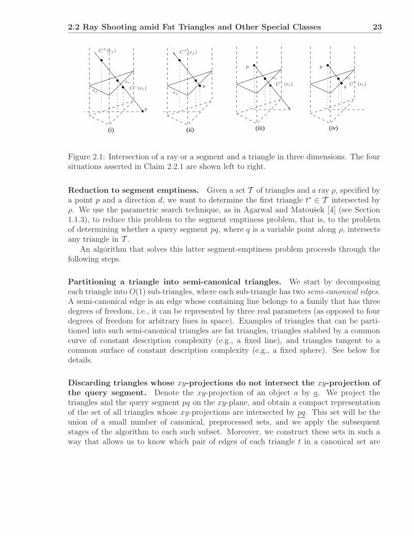
Claim 2.2.1 Given a non-vertical triangle ∆ with three edges e1, e2 and e3 and a non-vertical segment pq, all in R
3, then the segment pq intersects the triangle ∆ if and only if(exactly) one of the following conditions holds:
(i) pq intersects one positive curtain C+(ei) and one negative curtain C−(ej) of twodistinct respective edges ei, ej of ∆.
(ii) One of the endpoints p,q is below ∆ and pq intersects one positive curtain C+(ei)of ∆.
(iii) One of the endpoints is above ∆ and pq intersects one negative curtain C−(ei) of∆.
(iv) p is above ∆ and q is below ∆ or vice versa.
Proof: Straightforward; see Figure 2.1.
2.2.2 Overview of the algorithm
We first sketch the outline of our algorithm and then describe it in detail.
2.2 Ray Shooting amid Fat Triangles and Other Special Classes 23
(ii)(i) (iii) (iv)
p
p
C+(ej)
ej ej
C+(ej)
ei
C−(ei)
p
C−(ei)
ei
p
C−(ei)
ei
q
Figure 2.1: Intersection of a ray or a segment and a triangle in three dimensions. The foursituations asserted in Claim 2.2.1 are shown left to right.
Reduction to segment emptiness. Given a set T of triangles and a ray ρ, specified bya point p and a direction d, we want to determine the first triangle t∗ ∈ T intersected byρ. We use the parametric search technique, as in Agarwal and Matousek [4] (see Section1.1.3), to reduce this problem to the segment emptiness problem, that is, to the problemof determining whether a query segment pq, where q is a variable point along ρ, intersectsany triangle in T .
An algorithm that solves this latter segment-emptiness problem proceeds through thefollowing steps.
Partitioning a triangle into semi-canonical triangles. We start by decomposingeach triangle into O(1) sub-triangles, where each sub-triangle has two semi-canonical edges.A semi-canonical edge is an edge whose containing line belongs to a family that has threedegrees of freedom, i.e., it can be represented by three real parameters (as opposed to fourdegrees of freedom for arbitrary lines in space). Examples of triangles that can be parti-tioned into such semi-canonical triangles are fat triangles, triangles stabbed by a commoncurve of constant description complexity (e.g., a fixed line), and triangles tangent to acommon surface of constant description complexity (e.g., a fixed sphere). See below fordetails.
Discarding triangles whose xy-projections do not intersect the xy-projection ofthe query segment. Denote the xy-projection of an object a by a. We project thetriangles and the query segment pq on the xy-plane, and obtain a compact representationof the set of all triangles whose xy-projections are intersected by pq. This set will be theunion of a small number of canonical, preprocessed sets, and we apply the subsequentstages of the algorithm to each such subset. Moreover, we construct these sets in such away that allows us to know which pair of edges of each triangle t in a canonical set are

24 Ray Shooting and Stone Throwing
intersected by the segment in the projection. At least one of these edges is necessarily semi-canonical; we call it et
c, and call the other edge etr. We also collect in canonical sets triangles
whose projections contain one or two endpoints of pq. Handling such triangles is somewhatsimpler than triangles of the former kind. This is a fairly standard range searching task,and can be answered by constructing a multi-level structure, where each level checks for oneof a conjunction of conditions. As mentioned in Section 1.1.2, the total complexity of thestorage needed by the structure is comparable with that of its most space-consuming level,and the time needed to answer a query is comparable with the query cost of its costliestlevel. The storage requirement of this structure in our case is O∗(n), and the query time isO∗(n1/2). See [1] for examples of similar structures. In the remainder of this overview weonly consider canonical sets of the former kind.
Checking for intersection with curtains. We next need to test whether there existsa triangle t∗ in a given canonical set such that the query segment intersects the positivecurtain C+(et
c) and the negative curtain C−(etr). The symmetric case, involving C−(et
c)and C+(et
r), is handled similarly.We first collect all triangles t in a canonical subset so that pq intersects the positive
curtain C+(etc) erected from the semi-canonical edge et
c of t. The output is again a union ofa small number of canonical sets. The fact that the edges et
c are semi-canonical allows us torepresent these curtains as points in a 3-dimensional space (rather than 4-dimensional asin the case of general curtains or lines in space), and this property is crucial for obtainingthe improved query time.
Finally, for each of the new canonical sets, we test whether the segment intersectsthe negative curtain C−(et
r), erected over the other edge etr of at least one triangle in
the set. This step is done using the (standard) representation of lines in R3 as points or
hyperplanes in the 5-dimensional Plucker space, and exploiting the linear structure of thisrepresentation [24]. Symmetrically, we test, over all canonical sets, whether pq intersectsthe negative curtain C−(et
c) and the positive curtain C+(etr) of at least one triangle t.
Any successful test at this stage implies that pq intersects a triangle in T . We also test forintersections of the types (ii)−(iv) listed in Claim 2.2.1 using similar techniques (describedin more detail below).
As our analysis will show, this multi-level structure uses O∗(n) space and preprocessingand can answer queries in O∗(n2/3) time.
2.2.3 Partitioning a triangle into semi-canonical triangles
Fat Triangles
Assume that the triangles are not “too vertical”. This assumption is needed to assure thata fat triangle in 3-space has a fat projection on the xy-plane. More formally, we assumethat the angle formed between the xy-plane and the plane that supports any triangle in T is
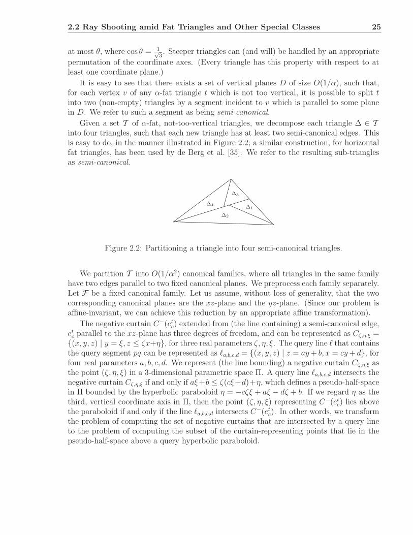
2.2 Ray Shooting amid Fat Triangles and Other Special Classes 25
at most θ, where cos θ = 1√3. Steeper triangles can (and will) be handled by an appropriate
permutation of the coordinate axes. (Every triangle has this property with respect to atleast one coordinate plane.)
It is easy to see that there exists a set of vertical planes D of size O(1/α), such that,for each vertex v of any α-fat triangle t which is not too vertical, it is possible to split tinto two (non-empty) triangles by a segment incident to v which is parallel to some planein D. We refer to such a segment as being semi-canonical.
Given a set T of α-fat, not-too-vertical triangles, we decompose each triangle ∆ ∈ Tinto four triangles, such that each new triangle has at least two semi-canonical edges. Thisis easy to do, in the manner illustrated in Figure 2.2; a similar construction, for horizontalfat triangles, has been used by de Berg et al. [35]. We refer to the resulting sub-trianglesas semi-canonical.
∆4
∆3
∆1
∆2
Figure 2.2: Partitioning a triangle into four semi-canonical triangles.
We partition T into O(1/α2) canonical families, where all triangles in the same familyhave two edges parallel to two fixed canonical planes. We preprocess each family separately.Let F be a fixed canonical family. Let us assume, without loss of generality, that the twocorresponding canonical planes are the xz-plane and the yz-plane. (Since our problem isaffine-invariant, we can achieve this reduction by an appropriate affine transformation).
The negative curtain C−(etc) extended from (the line containing) a semi-canonical edge,
etc parallel to the xz-plane has three degrees of freedom, and can be represented as Cζ,η,ξ =(x, y, z) | y = ξ, z ≤ ζx+η, for three real parameters ζ, η, ξ. The query line ℓ that containsthe query segment pq can be represented as ℓa,b,c,d = (x, y, z) | z = ay + b, x = cy + d, forfour real parameters a, b, c, d. We represent (the line bounding) a negative curtain Cζ,η,ξ asthe point (ζ, η, ξ) in a 3-dimensional parametric space Π. A query line ℓa,b,c,d intersects thenegative curtain Cζ,η,ξ if and only if aξ+b ≤ ζ(cξ+d)+η, which defines a pseudo-half-spacein Π bounded by the hyperbolic paraboloid η = −cζξ + aξ − dζ + b. If we regard η as thethird, vertical coordinate axis in Π, then the point (ζ, η, ξ) representing C−(et
c) lies abovethe paraboloid if and only if the line ℓa,b,c,d intersects C−(et
c). In other words, we transformthe problem of computing the set of negative curtains that are intersected by a query lineto the problem of computing the subset of the curtain-representing points that lie in thepseudo-half-space above a query hyperbolic paraboloid.
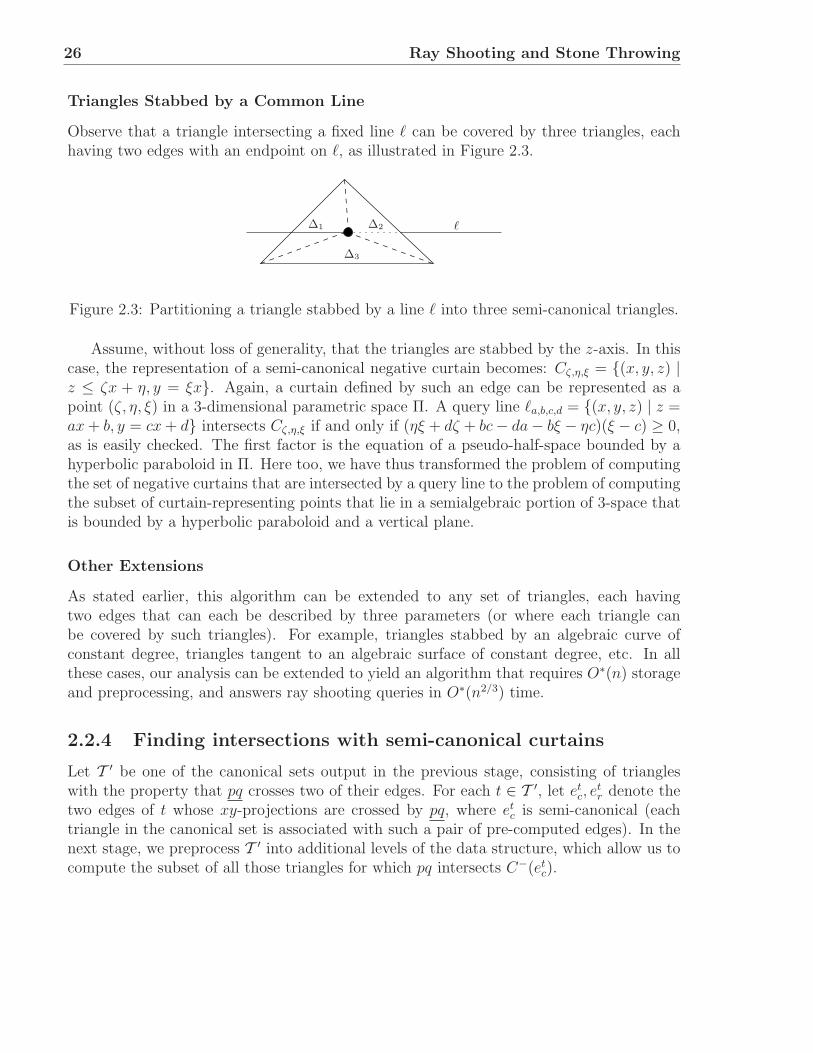
26 Ray Shooting and Stone Throwing
Triangles Stabbed by a Common Line
Observe that a triangle intersecting a fixed line ℓ can be covered by three triangles, eachhaving two edges with an endpoint on ℓ, as illustrated in Figure 2.3.
∆1 ∆2
∆3
ℓ
Figure 2.3: Partitioning a triangle stabbed by a line ℓ into three semi-canonical triangles.
Assume, without loss of generality, that the triangles are stabbed by the z-axis. In thiscase, the representation of a semi-canonical negative curtain becomes: Cζ,η,ξ = (x, y, z) |z ≤ ζx + η, y = ξx. Again, a curtain defined by such an edge can be represented as apoint (ζ, η, ξ) in a 3-dimensional parametric space Π. A query line ℓa,b,c,d = (x, y, z) | z =ax + b, y = cx + d intersects Cζ,η,ξ if and only if (ηξ + dζ + bc − da − bξ − ηc)(ξ − c) ≥ 0,as is easily checked. The first factor is the equation of a pseudo-half-space bounded by ahyperbolic paraboloid in Π. Here too, we have thus transformed the problem of computingthe set of negative curtains that are intersected by a query line to the problem of computingthe subset of curtain-representing points that lie in a semialgebraic portion of 3-space thatis bounded by a hyperbolic paraboloid and a vertical plane.
Other Extensions
As stated earlier, this algorithm can be extended to any set of triangles, each havingtwo edges that can each be described by three parameters (or where each triangle canbe covered by such triangles). For example, triangles stabbed by an algebraic curve ofconstant degree, triangles tangent to an algebraic surface of constant degree, etc. In allthese cases, our analysis can be extended to yield an algorithm that requires O∗(n) storageand preprocessing, and answers ray shooting queries in O∗(n2/3) time.
2.2.4 Finding intersections with semi-canonical curtains
Let T ′ be one of the canonical sets output in the previous stage, consisting of triangleswith the property that pq crosses two of their edges. For each t ∈ T ′, let et
c, etr denote the
two edges of t whose xy-projections are crossed by pq, where etc is semi-canonical (each
triangle in the canonical set is associated with such a pair of pre-computed edges). In thenext stage, we preprocess T ′ into additional levels of the data structure, which allow us tocompute the subset of all those triangles for which pq intersects C−(et
c).
2.2 Ray Shooting amid Fat Triangles and Other Special Classes 27
We choose some parameter r ≤ n, and obtain a partition of the (set of points in Πrepresenting the) semi-canonical lines into m = O(r) subsets L1, . . . , Lm, such that eachset consists of O(n/r) points, and the following property holds. For each query line ℓ,let σℓ denote the surface bounding the parametric region σ+
ℓ of all negative semi-canonicalcurtain crossed by ℓ. Then σℓ separates the points of at most O∗(r2/3) sets. This partitioningfollows, in a routine manner, from the technique of Agarwal and Matousek [5] for rangesearching with semialgebraic sets, which, in the special case at hand, uses the fact thatthe arrangement of any t of these surfaces can be decomposed into O∗(t3) subcells, each ofconstant description complexity.
Given a query surface that represents the query line ℓ, every set Li either lies entirelyin the “crossing region” σ+
ℓ , lies entirely outside σ+ℓ , or is separated by σℓ. If Li ∩ σ+
ℓ = ∅,we ignore Li. If Li ⊂ σ+
ℓ , we pass Li to the next level of the data structure. Otherwise werecurse into Li.
Using this structure, we output the set of all triangles that have a negative semi-canonical curtain intersected by pq (and have another edge whose projection is also in-tersected by pq), as the union of pre-computed sets of triangles. Similarly, we can output,in the same fashion, the set of all triangles that have a positive semi-canonical curtainintersected by pq.
Consider next the case where T ′ is a canonical set of triangles with the property thattheir xy-projections contain one endpoint of pq, say p, and have an edge whose projectionintersects pq. Rather than preprocessing curtain-representing points in Π, we preprocessthe set of planes in R
3 that contain the triangles of T ′, so that we can efficiently representthe set of all triangles in T ′ whose planes pass above a query point p (or below such apoint). To do so, we dualize 3-space, mapping these planes into points, and any querypoint into a query plane, where the task is to determine the set of all the dual points thatlie above the dual query plane. This is a standard three-dimensional range-query task [58],which can be done in much the same way as above, using query planes instead of querysurfaces, with the same asymptotic performance bounds.
Finally, consider the simplest case of all, where T ′ is a canonical set of triangles withthe property that their xy-projections contain both p and q. We preprocess T ′ exactly asin the preceding paragraph, and query it with the point p. Let T ′′ be a canonical subsetof the query output, consisting of triangles whose planes pass above p. We then need todetermine whether T ′′ contains a triangle whose plane passes below q, and then report anintersection of the type (iv) listed in Claim 2.2.1. This final task is easy to accomplish:we compute the lower envelope of the planes of the triangles in T ′′, which is a convexpolyhedron, and preprocess it for efficient point location queries, which determine whethera query point q lies above or below the envelope. Note that q lies above the envelope if andonly if it passes above a plane containing a triangle of T ′′. Putting n′′ = |T ′′|, this finaltask can be performed in O(n′′ log n′′) preprocessing time, O(n′′) storage, and O(log n′′)query time, see [67] for a survey.
28 Ray Shooting and Stone Throwing
2.2.5 Determining an intersection with ordinary curtains
We now describe the last level of our data structure, for the remaining types of canonicalsubsets, excluding those that correspond to case (iv) of Claim 2.2.1. The output of aquery segment pq, as it passes through the preceding levels, is a collection of canonicalprecomputed sets of triangles. Each such subset T ′′ has the property that pq intersectsC−(et
c), for every triangle t ∈ T ′′, or that p lies below every triangle t ∈ T ′′; moreover,the projection of pq onto the xy-plane intersects the projection of a second, not necessarilysemi-canonical, edge et
r of t. It is therefore sufficient to check whether pq intersects any ofthe corresponding positive curtains C+(et
r).
This task is equivalent to testing whether there exists a line in a given set of lines in3-space (namely, the extensions of the edges et
r) which passes below a query line (whichis the line containing pq). Equivalently, it suffices to test whether all the input lines passabove the query line.
This task can be accomplished by mapping the data lines to points, and the queryline to a hyperplane, in Plucker’s 5-space [24], and by applying Matousek’s algorithm forhalf-space emptiness detection [57]. This algorithm, which is based on the so-called shallowcutting lemma, runs in O(n1/22O(log∗ n)) time, with linear space and O(n log n) preprocessingtime.
The overall cost of the algorithm. The space requirement Σ(n) of any level in ourdata structure (including all the subsequent levels below it), for a set of n triangles, satisfiesthe recurrence:
Σ(n) = O(r)Σ′(n
r
)+ O(r)Σ
(n
r
),
where Σ′(n) is the space requirement of the next levels, for a set of n triangles. If Σ′(n) =O(n1+ε), for any ε > 0, then, choosing r to be a sufficiently large constant that dependson ε, one can show that Σ(n) = O(n1+ε), for any ε > 0, as well. Since Σ′(n) = O(n) atthe bottom level of the structure, this implies that the overall storage required by the datastructure is O(n1+ε), for any ε > 0. The preprocessing time obeys a similar recurrencewhose solution is also O(n1+ε). That is, both storage and preprocessing are O∗(n).
Similarly, the query time Q(n) of any level in our data structure, for a set of n triangles,satisfies the recurrence:
Q(n) = O(r) + O(r)Q′(n
r
)+ O∗(r2/3)Q
(n
r
),
where Q′(n) is the query time at the next levels (for n triangles). If Q′(n) = O(n2/3+ε) forany ε > 0 (it is O(1) at the bottom level of the structure), then, choosing r as above, andcalibrating the factor O∗(r2/3), it follows that Q(n) = O(n2/3+ε), for any ε > 0, as well.That is, Q(n) = O∗(n2/3). In conclusion, we thus obtain:
2.3 Stone Throwing 29
Theorem 2.2.2 The ray shooting problem amid n fat triangles in R3 can be solved with
a query time O∗(n2/3), using a data structure of size O∗(n), which can be constructed inO∗(n) time. The same bounds apply to each of the other special classes of triangles listedabove, such as triangles stabbed by a common line.
2.2.6 Trading space for query time
So far, we have only considered algorithms that use near-linear storage. At the other endof the spectrum, using O∗(n4) space and preprocessing, ray shooting queries for generaltriangles can be answered in logarithmic time [9, 35]; there are no known better bounds forthe special cases that we discuss. By combining these two solutions, a trade-off betweenstorage and query time can be obtained, as in [9, 27, 59]. The idea behind these techniquesis to build a partition-tree-like data structure, as described in the preceding sections, up toa certain depth. At that depth we apply the more space-consuming construction to eachof the subsets of triangles stored at the (new) leaves. For example, if we recurse up toa depth where there are O(nα) triangles in each leaf of the partition tree, then we needO∗(n1−αn4α) = O∗(n1+3α) space, and the query time is O∗((n1−α)2/3 log n) = O∗(n2/3−2/3α).This two-way construction has to be applied to each level of our data structure, but, asshown in [9, 27, 59], this does not affect the asymptotic form of the overall trade-off justnoted. Putting m = n1+3α, or nα = (m/n)1/3, the storage becomes O∗(m) and the querybecomes O∗(n2/3(m/n)−2/9) = O∗(n8/9/m2/9). In summary, we have shown:
Theorem 2.2.3 For any parameter n ≤ m ≤ n4, the ray shooting problem for a set of nfat triangles, or n triangles stabbed by a common line, or any of the other special cases ofSection 2.2.3, can be solved using O∗(m) space and preprocessing, and O∗(n8/9/m2/9) querytime.
2.3 Stone Throwing
The ships hung in the sky in much the same way that bricks don’t.(The Hitchhiker’s Guide to the Galaxy)
Next we study another problem of shooting along arcs amid triangles in three dimen-sions, which we refer to as stone throwing. In this problem we are given a set T of n(arbitrary) triangles in R
3, and we wish to preprocess them into a data structure that cananswer efficiently stone throwing queries, where each query specifies a point p ∈ R
3 and avelocity vector v ∈ R
3; these parameters define a parabolic trajectory traced by a stonethrown from p with initial velocity v under gravity (which we assume to be exerted inthe negative z-direction), and the query asks for the first triangle of T to be hit by thistrajectory.
30 Ray Shooting and Stone Throwing
The query has six degrees of freedom, but the parabola π that contains the stonetrajectory has only five degrees of freedom. Two of them define the vertical plane Vπ
(parallel to the z-axis) in which π lies, and three define the planar equation of π withinVπ. That is, we can specify the parabola, e.g., by the quintuple (a, b, c, d, e) that define theequations y = ax + b, z = cx2 + dx + e. (We ignore, for simplicity of presentation, thesimpler case where Vπ is parallel to the yz-plane.) Note that, under gravity, we have c < 0,i.e., π is concave.
Unlike our treatment of the case of ray shooting, we only consider here the basic casewhere the triangles of T are arbitrary, and present a solution that uses near-linear storageand preprocessing, and answers stone-throwing queries in time O∗(n3/4). These bounds areinteresting, since they are identical to the best bounds known for the general ray-shootingproblem, even though the stone-throwing problem seems to be harder than ray shooting,since it involves one additional degree of freedom. At present we do not know whether theproblem admits a faster solution for the special classes of triangles considered in the firstpart of the chapter. Moreover, at the other extreme end of the trade-off, where we wishto answer stone-throwing queries in O(log n) time, the best solution that we have requiresO∗(n5) storage, which is larger, by a factor of n, than the best known solution for theray-shooting problem. We omit in this chapter the description of this alternative solution.
Using the parametric searching technique, as in [4] and the preceding section, we canreduce the problem to testing emptiness of concave vertical parabolic arcs, in which wewish to determine whether such a query arc intersects any triangle in T .
Claim 2.3.1 Given a non-vertical triangle ∆, contained in a plane h, with three edges e1,e2 and e3, and given a parabolic arc pq contained in some concave vertical parabola π, anddelimited by the points p, q, all in R
3, then the arc pq intersects the triangle ∆ if and only if(exactly) one of the following conditions holds (in the first four conditions the intersectionconsists of a single point, and in the last three it consists of two points):
(1.i) pq intersects one positive curtain C+(ei) and one negative curtain C−(ej) of ∆.(1.ii) One endpoint, say p, lies below ∆, and pq intersects one positive curtain C+(ei)
of ∆.(1.iii) One endpoint, say p, lies above ∆, and pq intersects one negative curtain C−(ei)
of ∆.(1.iv) One endpoint lies above ∆, and the other endpoint lies below ∆.(2.i) The parabola π intersects the plane h, pq intersects two negative curtains C−(ei)
and C−(ej), at the respective intersection points p1 and p2, and S(p1) ≤ slope(h ∩ Vπ) ≤S(p2) (or vice versa), where S(x) is the slope of the tangent to π at point x, and slope(h∩Vπ)is the slope of this intersection line, where all slopes are defined within the vertical planeVπ.
(2.ii) One endpoint, say p, lies below ∆, π intersects the plane h, pq intersects onenegative curtain C−(ei) of ∆ at some point p1, and S(p1) ≤ slope(h ∩ Vπ) ≤ S(p), orS(p) ≤ slope(h ∩ Vπ) ≤ S(p1).
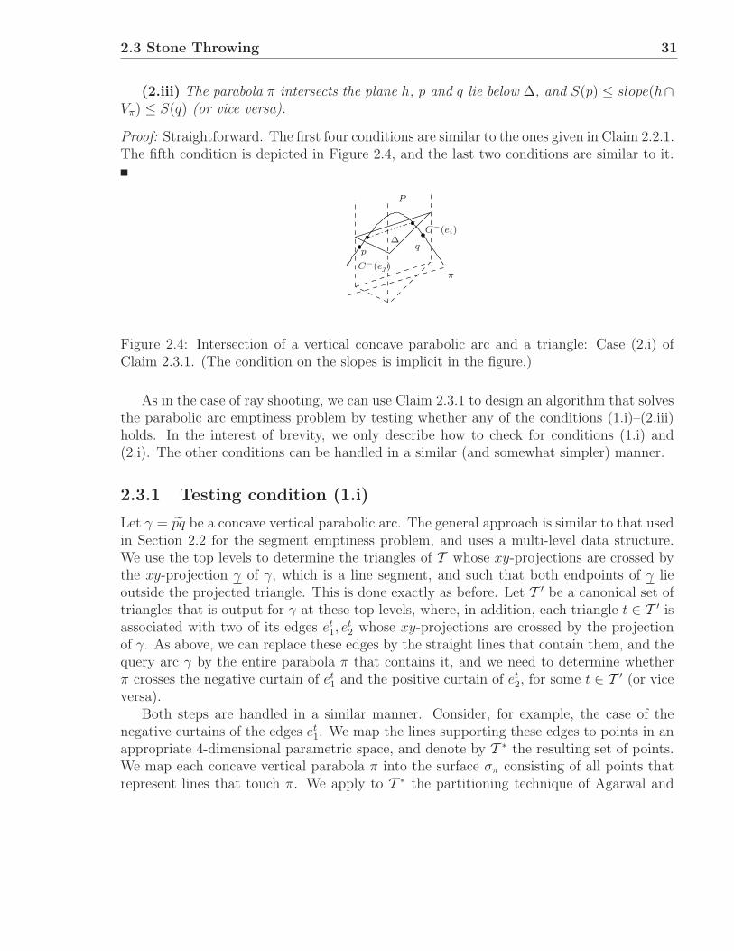
2.3 Stone Throwing 31
(2.iii) The parabola π intersects the plane h, p and q lie below ∆, and S(p) ≤ slope(h∩Vπ) ≤ S(q) (or vice versa).
Proof: Straightforward. The first four conditions are similar to the ones given in Claim 2.2.1.The fifth condition is depicted in Figure 2.4, and the last two conditions are similar to it.
C−(ei)
πC−(ej)
P
∆p
q
Figure 2.4: Intersection of a vertical concave parabolic arc and a triangle: Case (2.i) ofClaim 2.3.1. (The condition on the slopes is implicit in the figure.)
As in the case of ray shooting, we can use Claim 2.3.1 to design an algorithm that solvesthe parabolic arc emptiness problem by testing whether any of the conditions (1.i)–(2.iii)holds. In the interest of brevity, we only describe how to check for conditions (1.i) and(2.i). The other conditions can be handled in a similar (and somewhat simpler) manner.
2.3.1 Testing condition (1.i)
Let γ = pq be a concave vertical parabolic arc. The general approach is similar to that usedin Section 2.2 for the segment emptiness problem, and uses a multi-level data structure.We use the top levels to determine the triangles of T whose xy-projections are crossed bythe xy-projection γ of γ, which is a line segment, and such that both endpoints of γ lieoutside the projected triangle. This is done exactly as before. Let T ′ be a canonical set oftriangles that is output for γ at these top levels, where, in addition, each triangle t ∈ T ′ isassociated with two of its edges et
1, et2 whose xy-projections are crossed by the projection
of γ. As above, we can replace these edges by the straight lines that contain them, and thequery arc γ by the entire parabola π that contains it, and we need to determine whetherπ crosses the negative curtain of et
1 and the positive curtain of et2, for some t ∈ T ′ (or vice
versa).Both steps are handled in a similar manner. Consider, for example, the case of the
negative curtains of the edges et1. We map the lines supporting these edges to points in an
appropriate 4-dimensional parametric space, and denote by T ∗ the resulting set of points.We map each concave vertical parabola π into the surface σπ consisting of all points thatrepresent lines that touch π. We apply to T ∗ the partitioning technique of Agarwal and
32 Ray Shooting and Stone Throwing
Matousek [5], which partitions T ∗ into r subsets, each consisting of O(n/r) points, so thatany surface σπ separates the points in at most O∗(r3/4) subsets. This result depends onthe existence of a vertical decomposition of the four-dimensional arrangement of any msurfaces σπ into O∗(m4) elementary cells (see [5] and Chapter 4 for details), which followsfrom the result of Koltun [53]. We apply this partitioning step recursively, and obtain apartition tree, similar to those constructed earlier. Similar structures are constructed atthe next level, which handles positive curtains erected over the other edges et
2 of trianglesin each resulting canonical subset. Recall that at this stage we only need to determinewhether there exists a triangle t in the canonical subset T whose edge et
2 passes belowπ. With an appropriate parametrization this can be expressed as testing whether anypoint in T ∗ lies below the surface σπ. This test is simpler than the preceding one, butwe make no attempt to optimize it, and instead use the same partition tree as in thepreceding level. (See however Chapter 4 in which problems of this latter kind are studiedin detail, and where improved solutions are derived in several special instances.) We omitthe further straightforward details. Arguing as above, one can show that the overall datastructure requires O∗(n) storage and preprocessing, and tests for condition (1.i) in overalltime O∗(n3/4).
2.3.2 Testing condition (2.i)
This test is somewhat more involved than the preceding one. It also constructs a multi-leveldata structure, whose top levels are similar to the entire structure of the preceding datastructure. Using them, we can collect, for a query arc γ, canonical subsets of triangles, sothat, for each triangle t in each such set T ′, γ intersects the negative curtains erected overtwo designated edges et
1, et2 of t
In the next level, we collect those triangles t that also satisfy the condition that theparabola π containing γ intersects the plane containing t. This is done by mapping theplanes containing the triangles t ∈ T ′ to points in dual 3-space, and by mapping any queryparabola π to the surface σπ, consisting of all points that are dual to planes tangent to π.With an appropriate parametrization, the query seeks all the dual points which lie belowthe query surface σπ. Applying the range-searching technique of [5], we can output thesubset of the desired triangles as the union of a collection of canonical sets, as above. Sincethis level deals with points in 3-space, its performance is better than that of the precedingcurtain-intersection levels.
It remains to test, for each such output set T ′, whether there exists t ∈ T ′, such thatthe two slope conditions, over C−(et
1) and C−(et2), are satisfied. The next levels test for the
slope conditions. Consider the slope condition over C−(et1), for a triangle t in a canonical
subset T ′′ (that is, the condition S(p1) ≤ slope(h ∩ Vπ)). There are two slopes that needto be compared. The first is the slope S(p1) of the tangent to π at the point p1 where itcrosses C−(et
1). This slope depends only on two of the parameters that specify t, namelythe coefficients of the equation of the xy-projection of et
1. The second slope is that of the

2.3 Stone Throwing 33
line h ∩ Vπ, which depends only on the equation of the plane h containing t. Moreover,if the equation of this plane is z = ξx + ηy + ζ, then the slope is independent of ζ. Inother words, the overall slope condition can be expressed as a semialgebraic condition thatdepends on only four parameters that specify t. Hence, we can represent the triangles ofT ′′ as points in an appropriate 4-dimensional parametric space 1, and map each parabola πinto a semialgebraic set of constant description complexity in that space, which representsall triangles t for which π satisfies the slope condition over C−(et
1). We now apply thepartitioning technique of [5] for the set of points representing the triangles of T ′′ and forthe set of ranges corresponding to parabolas π, as just defined. (Again, since we are in 4-space, the bound of [53] allows us to apply the technique of [5], with the same performancebounds as in the testing of condition (1.i).) The slope condition over the other negativecurtains C−(et
2) is handled in the next and final level of the data structure, in exactly thesame way as just described. We omit the further technical but routine details of handlingthese levels, which are similar to those already discussed.
Since each level of the data structure deals with sets of points in some parametric spaceof dimension at most four, the preceding analysis implies that the overall query time isO∗(n3/4), and the storage remains O∗(n).
Extending these techniques to the other remaining five conditions of Claim 2.3.1, andomitting all further (but routine) details, we thus obtain:
Theorem 2.3.2 A set of n triangles in R3 can be preprocessed into a data structure of size
O∗(n) in time O∗(n), so that any stone-throwing query can be answered in time O∗(n3/4).
2.3.3 Shooting along bounded-degree algebraic arcs
As mentioned in Section 1.2.1 this result can be extended to shooting along arcs that aregraphs of univariate algebraic functions of constant maximum degree that lie in any verticalplane. We simply break such a graph into its (constant number of) maximal convex andconcave portions, at points where the second derivative vanishes. It is easily verified thatClaim 2.3.1 holds for any vertical concave arc and its symmetric counterpart holds for anyvertical convex arc. We can therefore apply a similar algorithm to detect whether a concaveor convex vertical arc intersects any triangle, and apply it to each of the O(1) concave andconvex portions of the query arc. This is done in essentially the same manner as in the stonethrowing algorithm, and we omit the routine details. Note that the algebraic degree of thequery arc does not affect the asymptotic performance bounds (but affects the constants ofproportionality). This is because the query arc is mapped into a surface in some parametricspace of dimension that depends only on the input triangles, and is therefore at most four,as above. We thus obtain:
1With an appropriate general position assumption, all these points will be distinct, although coincidentpoints can also be handled.
34 Ray Shooting and Stone Throwing
Theorem 2.3.3 A set of n triangles in R3 can be preprocessed into a data structure of size
O∗(n) in time O∗(n), so that shooting along any vertical algebraic arc of constant maximumdegree can be answered in time O∗(n3/4).
2.4 Conclusions
We have presented algorithms and data structures for answering various ray shooting (andstone throwing) queries. All these structures require O∗(n) storage and preprocessingtime, and answer a query in sub-linear time. Our results either improve upon previousbounds, or give the first published bounds for the problem. Our data structures are fairlystandard multi-level range searching structures, which make use of the partition techniqueof Matousek. In the most significant levels, the data is transformed into parametric spacewhere every line (extension of some triangle edge) is transformed into a point, and the queryline or curve (the extension of the query ray or arc) is transformed into a semialgebraicrange in that space. The query (at that particular level) then becomes a semialgebraicrange searching query, and is carried out using known techniques, such as that of [5].
The innovation of these structures comes from an observation that reduces the dimensionof the parametric space used at the critical level(s) of the structure. In the case of rayshooting amid special classes of triangles, this space is three-dimensional (as opposed tothe standard four dimensions), which results in O∗(n2/3) query time. In the case of stonethrowing amid general triangles, this space is four-dimensional, which results in O∗(n3/4)query time.
We did not manage to extend these ideas to improve the storage (and preprocessingtime) of data structures that answer queries in logarithmic time. In this other end of thespectrum, the standard approach is to represent a query ray (or its extension to a line) asa point in some parametric space. The triangle edges (or the lines that support them) aretransformed to (surfaces bounding) certain semialgebraic ranges in that parametric space.The data structure then answers a query by locating the cell of the arrangement of thesesurfaces that contains the query point. The fact that the surfaces can be represented byonly three parameters does not seem to help here—we still need to consider arrangements inthe 4-dimensional parametric space of lines in space (since the query line is not restricted,and can be any line in space). It is an intriguing open question whether the special structureof the arrangement can be exploited to reduce the storage cost.
Chapter 3
Inter-point Visibility over Terrains inTwo and Three Dimensions
... wrap it round your head to ward off noxious fumes or to avoid the gaze of theRavenous Bugblatter Beast of Traal (a mindboggingly stupid animal, it assumesthat if you can’t see it, it can’t see you — daft as a bush, but very ravenous).(The Hitchhiker’s Guide to the Galaxy)
3.1 Introduction
In this chapter we consider the following mutual visibility problem. We are given a setP of m points and a polygonal or polyhedral terrain T in two or three dimensions withn vertices, so that all the points of P lie above T . We present efficient algorithms thatdetermine whether all pairs of points of P are mutually visible, i.e., whether each pairp, q ∈ P has the property that the segment pq lies fully above T .
In Section 3.2 we present an algorithm for the planar case, which runs in O(m log m+n)time. In Section 3.3 we present an algorithm for the problem in three dimensions. We showthat in this case the problem is 3sum-hard, so our algorithm, which runs in O(nm log2 m)time, is likely to be nearly worst-case optimal.
3.2 Terrains in Two Dimensions
Consider first the planar case. Here the terrain T is simply an unbounded connected x-monotone polygonal path with n vertices, and P is a set of m points, all lying above T .As above, two points p, q are mutually visible if the segment pq does not pass below anyterrain vertex. A terrain vertex is a witness to the non-visibility of a pair p, q ∈ P ifit lies above the segment pq (with one point lying to its right and one lying to its left).
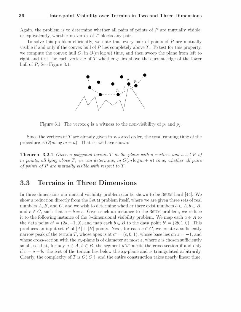
36 Inter-point Visibility over Terrains in Two and Three Dimensions
Again, the problem is to determine whether all pairs of points of P are mutually visible,or equivalently, whether no vertex of T blocks any pair.
To solve this problem efficiently, we note that every pair of points of P are mutuallyvisible if and only if the convex hull of P lies completely above T . To test for this property,we compute the convex hull C, in O(m log m) time, and then sweep the plane from left toright and test, for each vertex q of T whether q lies above the current edge of the lowerhull of P ; See Figure 3.1.
pj
piℓ
q
Figure 3.1: The vertex q is a witness to the non-visibility of pi and pj.
Since the vertices of T are already given in x-sorted order, the total running time of theprocedure is O(m log m + n). That is, we have shown:
Theorem 3.2.1 Given a polygonal terrain T in the plane with n vertices and a set P ofm points, all lying above T , we can determine, in O(m log m + n) time, whether all pairsof points of P are mutually visible with respect to T .
3.3 Terrains in Three Dimensions
In three dimensions our mutual visibility problem can be shown to be 3sum-hard [44]. Weshow a reduction directly from the 3sum problem itself, where we are given three sets of realnumbers A,B, and C, and we wish to determine whether there exist numbers a ∈ A, b ∈ B,and c ∈ C, such that a + b = c. Given such an instance to the 3sum problem, we reduceit to the following instance of the 3-dimensional visibility problem. We map each a ∈ A tothe data point a∗ = (2a,−1, 0), and map each b ∈ B to the data point b∗ = (2b, 1, 0). Thisproduces an input set P of |A| + |B| points. Next, for each c ∈ C, we create a sufficientlynarrow peak of the terrain T , whose apex is at c∗ = (c, 0, 1), whose base lies on z = −1, andwhose cross-section with the xy-plane is of diameter at most ε, where ε is chosen sufficientlysmall, so that, for any a ∈ A, b ∈ B, the segment a∗b∗ meets the cross-section if and onlyif c = a + b. the rest of the terrain lies below the xy-plane and is triangulated arbitrarily.Clearly, the complexity of T is O(|C|), and the entire construction takes nearly linear time.

3.3 Terrains in Three Dimensions 37
By construction, a ∈ A, b ∈ B and c ∈ C satisfy a + b = c if and only if a∗ andb∗ are non-visible with respect to T , with the peak at c∗ blocking their mutual visibility.Hence a subquadratic solution to the 3-dimensional mutual visibility problem would yielda subquadratic solution to the 3sum problem, so the problem is indeed 3sum-hard, asclaimed.
We therefore cannot hope for a subquadratic solution to the 3-dimensional mutualvisibility problem. In what follows we present a solution with nearly quadratic runningtime.
The algorithm checks, for each edge e of T , whether e blocks the visibility of any pair ofpoints of P . Consider then a fixed edge e. Project P and e on the xy-plane, and assume,without loss of generality, that the image e∗ of e lies on the y-axis; denote its endpoints bya and b, so that a is its bottom endpoint and b is its top endpoint. Let L (resp., R) denotethe set of points of P whose projections lie to the left (resp., to the right) of the y-axis.Denote by q∗ the xy-projection of a point q ∈ R
3, and let L∗ and R∗ denote the respectiveprojections of L and R on the xy-plane, that is, L∗ = q∗ | q ∈ L and R∗ = q∗ | q ∈ R.Let L0 ⊆ L and R0 ⊆ R be subsets with the property that for every p ∈ L0, q ∈ R0, thesegment p∗q∗ crosses e∗. We can then test whether e blocks the visibility of any pair inL0 × R0 as follows. Let ℓ be the line containing e (back in 3-space) and let p0 ∈ L0 bethe lowest point of L0 as “seen” from ℓ. That is, the plane through ℓ and p0 passes belowall the other points of L0. Similarly, let q0 ∈ R0 be the lowest point of R0 as seen from ℓ.Then, as is easily checked, e does not block the visibility of any pair in L0 ×R0 if and onlyif it does not block the visibility between p0 and q0. Hence, testing for this property canbe done in O(|L0| + |R0|) time.
The algorithm then considers the graph H ⊆ L×R whose edges connect those pairs (p, q)for which p∗q∗ intersects e∗, decomposes H into a union of complete bipartite subgraphs,and applies the preceding procedure to each subgraph.
To obtain the decomposition of H, let a and b denote the endpoints of e∗; See Figure3.2. We store the points of R in a 2-dimensional range tree, where the points are stored inthe primary tree in the order of the slopes of the lines connecting their xy-projections witha. At each node v of the primary tree, we store a secondary range tree of the points storedat the subtree rooted at v, so that the points are stored at the secondary tree in the orderof the slopes of the lines connecting their xy-projections with b. Given a point l ∈ L, wecan query the two-level range tree with l, to compute the set of all points r ∈ R, for whichl∗r∗ crosses e∗, as a disjoint union of O(log2 m) precomputed canonical subsets. Next, weassociate with each canonical secondary subset Ri ⊂ R a subset Li ⊂ L, consisting of all thepoints l ∈ L for which Ri is one of the subsets of R whose union is the output to the querywith l. Finally, we test the visibility between each pair Li × Ri by the explicit proceduredescribed above, in O(|Li| + |Ri|) time. Hence, testing the visibility of L × R across e cantherefore be performed in time O(
∑i |Li| +
∑ |Ri|). Since each point l ∈ L and r ∈ Rappears in at most O(log2 |R|) pairs Li × Ri, the overall cost is O((|L| + |R|) log2 |R|).
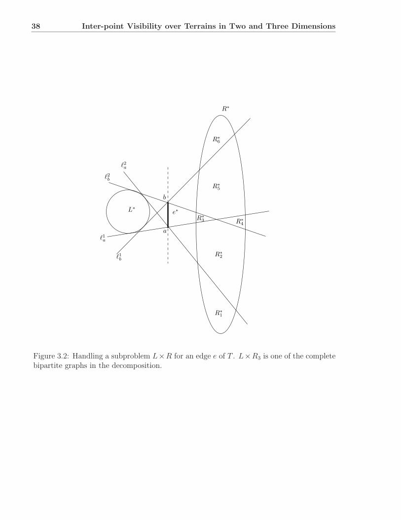
38 Inter-point Visibility over Terrains in Two and Three Dimensions
e∗L∗
R∗
1
R∗
2
R∗
4
R∗
R∗
6
R∗
5
a
ℓ1b
ℓ2b
ℓ2a
ℓ1a
b
R∗
3
Figure 3.2: Handling a subproblem L×R for an edge e of T . L×R3 is one of the completebipartite graphs in the decomposition.
3.3 Terrains in Three Dimensions 39
Repeating this procedure to each edge e of T , we get a procedure, with O(nm log2 m)running time, for solving the mutual visibility problem. We note that the storage used bythe algorithm is O(n) (to store the terrain) plus O(m log m) which is the storage used bya single 2-dimensional range tree. That is, we have shown:
Theorem 3.3.1 Given a polyhedral terrain T in 3-space with n vertices and a set P ofm points, all lying above T , we can determine, in O(nm log2 m) time and O(m log m + n)space, whether all pairs of points of P are mutually visible with respect to T .

40 Inter-point Visibility over Terrains in Two and Three Dimensions
Chapter 4
Emptiness and Reporting Querieswith Semialgebraic Ranges and TheirApplications
For thousands more years the mighty ships tore across the empty wastes ofspace and finally dived screaming on to the first planet they came across —which happened to be the Earth — where due to a terrible miscalculation ofscale the entire battle fleet was accidentally swallowed by a small dog.(The Hitchhiker’s Guide to the Galaxy)
4.1 Overview
In this chapter we extend Matousek’s technique for half-space emptiness queries to moregeneral semialgebraic ranges. In a typical range emptiness searching (resp., reporting)problem, we are given a set P of n points in R
d, and wish to preprocess it into a datastructure that supports efficient range emptiness (resp., reporting) queries, in which wespecify a range σ, which, in general, is a semialgebraic set in R
d of constant descriptioncomplexity, and wish to determine whether P ∩ σ = ∅, or to report all the points inP ∩σ. Range emptiness searching and reporting arise in many applications, and have beentreated by Matousek [57] in the special case where the ranges are half-spaces bounded byhyperplanes. As shown in [57], the two problems are closely related, and have solutions(for the case of half-spaces) with similar performance bounds. In this chapter we extendthe analysis to general semialgebraic ranges, and show how to adapt Matousek’s technique,without the need to linearize the ranges into a higher-dimensional space. This yields moreefficient solutions to several useful problems, and we demonstrate the new technique in fourapplications, with the following results:
(i) We present an algorithm for ray shooting amid n balls in R3, which uses O(n) storage
42 Emptiness and Reporting Queries with Semialgebraic Ranges
and O∗(n) preprocessing, and answers a query in O∗(n2/3) time, improving the previousbound of O∗(n3/4).
(ii) We present an algorithm that preprocesses, in O∗(n) time, a set P of n points in R3
into a data structure with O(n) storage, so that, for any query line ℓ (or, for that matter,any simply-shaped convex set), the point of P farthest from ℓ can be computed in O∗(n1/2)time. This improves the solution of [5] with query time O∗(n2/3). This in turn yieldsan algorithm that computes the largest-area triangle spanned by P in time O∗(n26/11), aswell as similar nontrivial algorithms for computing the largest-perimeter or largest-heighttriangle spanned by P .
(iii) We present an algorithm that preprocesses, in O∗(n) time, a set P of n points inR
2 into a data structure, so that, for any query α-fat triangle ∆ (i.e., a triangle all of whoseangles are at least α; see also Chapter 2), we can determine whether ∆ ∩ P is empty. Thealgorithm uses O(n) storage and can answer a query in O∗(1) time, that is, O(nε) time forany ε > 0. The previous solution for this problem uses O(n log2 n) storage and answersa query in O(log3 n) time. Alternatively, we can report, in O(nε + k) time, the points of∆ ∩ P , where k = |∆ ∩ P | and ε > 0 is arbitrary.
(iv) Finally we present an algorithm that preprocesses, in O∗(n) time, a set P of npoints in R
2 into a data structure with O(n) storage, so that, given any query semidisk c,or a circular cap larger than a semidisk,1 we can determine, in O∗(1) time, whether c ∩ Pis empty, or report the k points in c ∩ P in O∗(1) + O(k) time.
Adapting the recent techniques of [15, 16, 17], we can turn our solutions into efficient al-gorithms for approximate range counting (with small relative error) for the cases mentionedabove. Since the technical details of this extension are somewhat involved, we dedicate aseparate chapter (Chapter 5) to this extension.
Most of the special notation used in this chapter has been introduced in Chapter 1 (seein particular Section 1.1).
Our technique is closely related to the notions of nearest- or farthest-neighbor general-ized Voronoi diagrams, and of the union or intersection of geometric objects, where sharperbounds on the combinatorial complexity of these structures (or, more precisely, on the sizeof an elementary-cell decomposition of the corresponding portion of space; see below) yieldfaster range emptiness searching or reporting algorithms.
The function ζ(r). In Lemma 4.2.1 and Theorem 4.2.2, we use a function ζ(r) thatbounds the number of elementary cells in a decomposition of the complement of the unionof any r ranges of Γ. (See Section 1.1.7.) We assume that ζ(r) is “well behaved”, in thesense that for each c > 0 there exists c′ > 0 such that ζ(cr) ≤ c′ζ(r) for every r. Wealso assume that ζ(r) = Ω(r). Both assumptions are natural and hold in practically allapplications.
1Actually, it suffices to assume that the query caps are such that their central angles are at least someconstant positive angle; see Section 4.5.
4.2 Semialgebraic Range Reporting or Emptiness Searching 43
4.2 Semialgebraic Range Reporting or Emptiness
Searching
Shallow cutting in the semialgebraic case. We begin by extending the shallow cut-ting lemma of Matousek [57] to the more general setting of semialgebraic ranges. Thisextension is fairly straightforward, although it involves several technical steps that deserveto be highlighted. The analysis makes use of the notations introduced in Chapter 1, suchas elementary cells and elementary cell partition.
Lemma 4.2.1 (Extended Shallow Cutting Lemma) Let Γ be a collection of n semi-algebraic ranges in R
d. Assume that the complement of the union of any subset of m rangesin Γ can be decomposed into at most ζ(m) elementary cells, for a well-behaved function ζas above. Then, for any r ≤ n, there exists a (1/r)-cutting Ξ with the following properties:(i) The union of the cells of Ξ contains the complement of the union of Γ.(ii) Ξ consists of O(ζ(r)) elementary cells.(iii) The complement of the union of the cells of Ξ is contained in a union of O(r) rangesin Γ.
See Figure 4.1 for an illustration.
Proof: The proof is a fairly routine adaptation of the proof in [57]. We employ a variant ofthe method of Chazelle and Friedman [25] for constructing the cutting. Let Γ′ be a randomsample of O(r) ranges of Γ, and let E ′ denote the complement of the union of Γ′. Byassumption, E ′ can be decomposed into at most O(ζ(r)) elementary cells. The resultingcollection Ξ of these cells is such that their union clearly contains the complement of theunion of Γ. Moreover, the complement of the union of Ξ is the union of the O(r) ranges ofΓ′. Hence, Ξ satisfies all three conditions (i)–(iii), but it may fail to be a (1/r)-cutting.
This latter property is enforced as in [25], by further decomposing each cell τ of Ξ thatis crossed by more than n/r ranges of Γ, using additional subsamples from the surfacesthat cross τ . Specifically, for each cell τ of Ξ, let Γτ denote the subset of those ranges inΓ that cross τ , and put ξτ = |Γτ |r/n. If ξτ > 1, we sample q = O(ξτ log ξτ ) ranges fromΓτ , construct the complement of the union of these ranges, decompose it into at most ζ(q)elementary cells, and clip them to within τ . The resulting collection Ξ′ of subcells, over allcells τ of the original Ξ, clearly satisfies (i). The analysis of [25] (see also [7]) establishesan exponential decay property on the number of cells of Ξ that are crossed by more thanξn/r ranges, as a function of ξ. Specifically, as in [7], the expected number of such cellsis O(2−ξ
Eζ(|Γ′′|)), where Γ′′ is another random sample of Γ, where each member of Γis chosen with probability r
nξ. This property implies, as usual [25], that Ξ′ is (with high
probability) a (1/r)-cutting, and it also implies that the size of Ξ′ is still O(ζ(r)), assumingζ to be well behaved. Since we have only refined the original cells of Ξ, the number ofranges that cover the complement of the union of the final cells is still O(r).
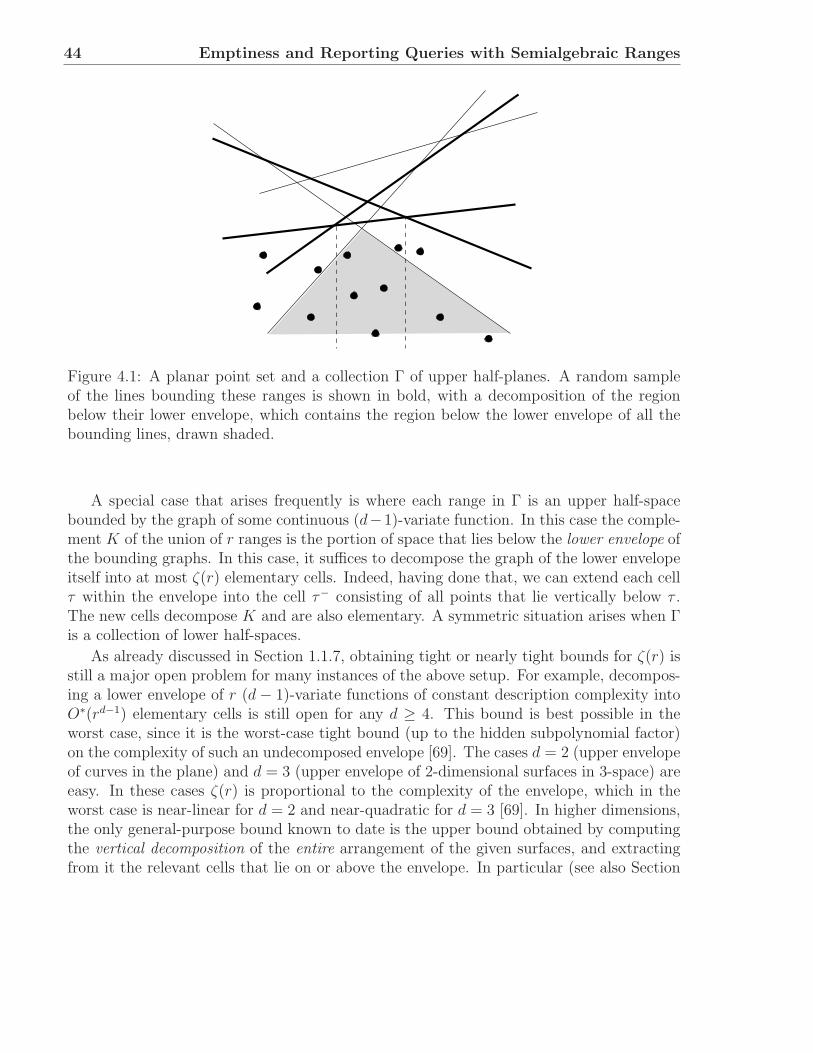
44 Emptiness and Reporting Queries with Semialgebraic Ranges
Figure 4.1: A planar point set and a collection Γ of upper half-planes. A random sampleof the lines bounding these ranges is shown in bold, with a decomposition of the regionbelow their lower envelope, which contains the region below the lower envelope of all thebounding lines, drawn shaded.
A special case that arises frequently is where each range in Γ is an upper half-spacebounded by the graph of some continuous (d−1)-variate function. In this case the comple-ment K of the union of r ranges is the portion of space that lies below the lower envelope ofthe bounding graphs. In this case, it suffices to decompose the graph of the lower envelopeitself into at most ζ(r) elementary cells. Indeed, having done that, we can extend each cellτ within the envelope into the cell τ− consisting of all points that lie vertically below τ .The new cells decompose K and are also elementary. A symmetric situation arises when Γis a collection of lower half-spaces.
As already discussed in Section 1.1.7, obtaining tight or nearly tight bounds for ζ(r) isstill a major open problem for many instances of the above setup. For example, decompos-ing a lower envelope of r (d − 1)-variate functions of constant description complexity intoO∗(rd−1) elementary cells is still open for any d ≥ 4. This bound is best possible in theworst case, since it is the worst-case tight bound (up to the hidden subpolynomial factor)on the complexity of such an undecomposed envelope [69]. The cases d = 2 (upper envelopeof curves in the plane) and d = 3 (upper envelope of 2-dimensional surfaces in 3-space) areeasy. In these cases ζ(r) is proportional to the complexity of the envelope, which in theworst case is near-linear for d = 2 and near-quadratic for d = 3 [69]. In higher dimensions,the only general-purpose bound known to date is the upper bound obtained by computingthe vertical decomposition of the entire arrangement of the given surfaces, and extractingfrom it the relevant cells that lie on or above the envelope. In particular (see also Section
4.2 Semialgebraic Range Reporting or Emptiness Searching 45
1.1.8), for d = 4 the bound is ζ(r) = O∗(r4), as follows from the results of [53]. This leavesa gap of about a factor of r between this bound and the bound O∗(r3) on the complexityof the undecomposed envelope. For arbitrary d ≥ 4, the bound is ζ(r) = O∗(r2d−4), withprogressively increasing gaps from the lower bound Ω∗(rd−1). Of course, in certain specialcases, most notably the case of hyperplanes, as studied in [57], both the envelope and itsdecomposition have (considerably) smaller complexity, with asymptotically equal bound(namely O(r⌊d/2⌋)).
The situation with the complexity of the union of geometric objects is even worse. Whileconsiderable progress was recently made on many special cases in two and three dimensions(see [8] for a recent comprehensive survey), there are only very few sharp bounds on thecomplexity of unions in higher dimensions. Worse still, even when a sharp bound onthe complexity of the union is known, obtaining comparable bounds on the complexityof a decomposition of the complement of the union is a much harder problem (in d ≥ 3dimensions). As an example, the union of n infinite cylinders in 3-space is known to havenear-quadratic complexity [11, 42], but it is still an open problem whether its complementcan be decomposed into a near-quadratic number of elementary cells.
Partition theorem for shallow semialgebraic ranges. We next apply the new shal-low cutting lemma to construct an elementary cell partition of a given input point set P ,with respect to a specific (finite) set Q of ranges. This is done in a fairly similar way tothat in [5] (see also [57, 58]). A major difference in handling the semialgebraic case is theconstruction of a set Q of ranges (called a test-set, as in [5, 57, 58]) that will be (a) smallenough, and (b) representative of all shallow (or empty) ranges, in a sense discussed indetail below. The method given in [57] does not work in the general semialgebraic case,and different, sometimes ad-hoc approaches need to be followed.
The following theorem summarizes the main part of the construction (except for theconstruction of Q).
Theorem 4.2.2 (Extended Partition Theorem) Let P be a set of n points in Rd, let
Γ be a family of semialgebraic ranges of constant description complexity, and let 1 ≤ r < nbe fixed. Let Q be another finite collection (not necessarily a subset of Γ) of semialgebraicranges of constant description complexity with the following properties: (i) The ranges inQ are all (n/r)-shallow. (ii) The complement of the union of any m ranges of Q can bedecomposed into at most ζ(m) elementary cells, for any m. (iii) Any (n/r)-shallow rangeγ ∈ Γ can be covered by the union of at most δ ranges of Q, where δ is a constant.Then there exists an elementary cell partition Π of P , of size O(r), into subsets of sizebetween n/r and 2n/r, such that the crossing number of any (n/r)-shallow range in Γ withthe cells of Π is either O(r/ζ−1(r) + log r log |Q|), if there exists a fixed ε > 0 such thatζ(r)/r1+ε is monotone increasing, or O(r log r/ζ−1(r) + log r log |Q|), otherwise.
The proof, which, again, is similar to those in [5, 57, 58], proceeds through the following

46 Emptiness and Reporting Queries with Semialgebraic Ranges
steps. We first have:
Lemma 4.2.3 Let P be a set of n points in Rd, and 1 ≤ r < n a parameter. Let Q be
a set of (n/r)-shallow ranges, with the property that the complement of the union of anysubset of m ranges of Q can be decomposed into at most ζ(m) elementary cells, for any m.Then there exists a subset P ′ ⊆ P of at least n/2 points and an elementary cell partitionΠ = (P1, s1), . . . , (Pm, sm) for P ′ with n/r ≤ |Pi| ≤ 2n/r for all i, such that each rangeof Q crosses at most O(r/ζ−1(r) + log |Q|) cells si of Π.
Proof: We will inductively construct disjoint sets P1, . . . , Pm ⊂ P of size n/r (to simplifythe presentation we ignore the floor rounding) and elementary cells s1, . . . , sm such thatPi ⊆ si for each i. The construction terminates when |P1 ∪ · · · ∪ Pm| ≥ n/2. Supposethat P1, . . . , Pi−1 have already been constructed, and set P ′
i := P \ ⋃j<i Pj. We construct
Pi as follows: For a range σ ∈ Q, let κi(σ) denote the number of cells among s1, . . . , si−1
crossed by σ. We define a weighted collection (Q,wi) of ranges, so that each range σ ∈ Qappears with weight (or multiplicity) wi(σ) = 2κi(σ). We put wi(Q) =
∑σ∈Q wi(σ). By
Lemma 4.2.1 and by our assumption that the function ζ(r) is well behaved, there exists a(1/t)-cutting Ξi for the weighted collection (Q,wi) of size at most r/4, for an appropriatechoice of t = c1ζ
−1(r), for some constant c1 > 0, with the following properties: The unionof Ξi contains the complement of the union of Q, and the complement of the union of Ξi
is contained in the union of O(t) = c2t ranges of Q, for some constant c2 > 0. Since allthese ranges are (n/r)-shallow, the number of points of P not in the union of Ξi is at mostc2t · (n/r) = n · c2(c1ζ
−1(r))/r, and our assumption that ζ(r) ≥ r imply that this is smallerthan n/4, if we choose t appropriately (i.e., choose c1 such that c2c1 < 1/4). Since weassume that |P ′
i | ≥ n/2, it follows that at least n/4 points of P ′i lie in the union of the at
most r/4 cells of Ξi. By the pigeonhole principle, there is a cell si of Ξi containing at leastn/r points of P ′
i . We take Pi to be some subset of P ′i ∩ si of size exactly n/r, and take si
to be the cell in the partition which contains Pi.
We next establish the asserted bound on the crossing numbers between the rangesof Q and the elementary cells s1, . . . , sm, in the following standard manner. The finalweight wm(σ) of a range σ ∈ Q with crossing number κ(σ) (with respect to the finalpartition) is 2κ(σ). On the other hand, each newly added cell si is crossed by ranges ofQ of total weight O(wi(Q)/t) = O(wi(Q)/ζ−1(r)), because si is an elementary cell of thecorresponding weighted (1/t)-cutting Ξi. The weight of each of these crossing ranges isdoubled at the i-th step, and the weight of all the other ranges remains unchanged. Thuswi+1(Q) ≤ wi(Q)(1 + O(1/ζ−1(r))). Hence, for each range σ ∈ Q we have
wm(σ) ≤ wm(Q) ≤ |Q|(
1 + O
(1
ζ−1(r)
))m
= |Q|(
1 + O
(1
ζ−1(r)
))O(r)
≤ |Q|eO(r/ζ−1(r)),
and thus κ(σ) = log wm(σ) = O(r/ζ−1(r) + log |Q|).
4.2 Semialgebraic Range Reporting or Emptiness Searching 47
Discussion. The limitation of Lemma 4.2.3 is that the bound that it derives (a) appliesonly to ranges in Q, and (b) includes the term log |Q|. An ingenious component of theanalysis in [57] overcomes both problems, by choosing a test set Q of ranges whose sizeis only polynomial in r (and, in particular, is independent of n), which is neverthelesssufficiently representative of all shallow ranges, in the sense that the crossing number ofany (n/r)-shallow range is O(maxκ(σ) | σ ∈ Q). This implies that Lemma 4.2.3 holdsfor all shallow ranges, with the stronger bound which does not involve log |Q| (assumingthat r/ζ−1(r) dominates the polylogarithmic term log |Q|).
Unfortunately, the technique of [57] does not extend to the case of semialgebraic ranges,as it crucially relies on the linearity of the ranges.2 The following lemma gives a sufficientcondition for a test set Q to be representative of the relevant shallow ranges, in the sensethat Q satisfies the assumptions made in Theorem 4.2.2. That is:
Lemma 4.2.4 Let P be a set of n points in Rd, and let Γ be a family of semialgebraic
ranges with constant description complexity. Consider an elementary-cell partition Π =(P1, s1), . . . , (Pr, sr) of P such that n/r ≤ |Pi| ≤ 2n/r for each i. Let Q be a finite set of(n/r)-shallow ranges (not necessarily ranges of Γ), so that the maximal crossing number ofa range q ∈ Q with respect to Π is κ. Then, for any range γ ∈ Γ which is contained in theunion of at most δ ranges of Q (for some constant δ), the crossing number of γ is at most(κ + 1)δ.
Proof: Let γ ∈ Γ be a range for which there exist δ ranges q1, . . . , qδ of Q such thatγ ⊆ q1 ∪ · · · ∪ qδ. Then, if γ crosses a cell si of Π, then at least one of the covering rangesqj must either cross si or fully contain si. The number of cells of Π that can be crossedby any single qj is at most κ, and each qj can fully contain at most one cell of Π (becauseqj is (n/r)-shallow).3 Hence, the overall number of cells of Π that γ can cross is at most(κ + 1)δ, as asserted.
Proof of Theorem 4.2.2. Apply Lemma 4.2.3 to the input set P0 = P , with parameterr0 = r. This yields an elementary-cell partition Π0 for (at least) half of the points of P0,which satisfies the properties of that lemma. Let P1 denote the set of the remaining pointsof P0, and set r1 = r0/2. Apply Lemma 4.2.3 again to P1 with parameter r1, obtaining anelementary cell partition Π1 for (at least) half of the points of P1. We iterate this processk = O(log r) times, until the set Pk has fewer than n/r points. We take Π to be the unionof all the elementary-cell partitions Πi formed so far, together with one large cell containing
2It uses point-hyperplane duality, and exploits the fact that a half-space (bounded by a hyperplane) in-tersects a simplex if and only if it contains a vertex of the simplex, which is false in the general semialgebraiccase.
3By choosing a slightly smaller value for r in the construction of the partition, we can even rule out thepossibility that a range qj fully contains a cell of Π. This however has no effect on the asymptotic boundsthat the analysis derives.
48 Emptiness and Reporting Queries with Semialgebraic Ranges
all the remaining points of Pk. The resulting elementary-cell partition of P consists of atmost 1 + r + r/2 + r/4 + . . . ≤ 2r subsets, each of size at most 2n/r (the sizes are all equalto n/r except for the last set). The crossing number of a range in Q is, by Lemma 4.2.3,
O
(log r∑
i=1
((r/2i)/ζ−1(r/2i) + log |Q|
))
.
Our assumptions on ζ imply that if there exists an ε > 0 such that ζ(r)/r1+ε is monotoneincreasing, then the first terms add up to O(r/ζ−1(r)); otherwise we can bound theirsum by O(r log r/ζ−1(r)). Hence, by the properties of Q and by Lemma 4.2.4, the crossingnumber of any (n/r)-shallow range, and in particular any empty range, is also O(r/ζ−1(r)+log |Q| log r) or O(r log r/ζ−1(r) + log |Q| log r), respectively.
Partition trees and reporting or emptiness searching. As in the classical workson range searching [5, 57, 58], we choose r to be a sufficiently large constant and applyTheorem 4.2.2 recursively, and obtain a partition tree T , where each node v of T storesa subset Pv of P and an elementary cell σv enclosing Pv. (The root stores the entire Pand some sufficient large enclosing cell.) The children of a node v are obtained from anelementary cell partition of Pv—each of them stores one of the resulting subsets of Pv andits enclosing cell. At each leaf, the size of the subset that it stores is O(r).
Testing a range γ for emptiness is done by searching with γ in T . At each visited nodev, where γ ∩ σv 6= ∅, we test whether γ ⊇ σv, in which case γ is not empty. Otherwise, wefind the children of v whose cells are intersected by γ. If there are too many of them (morethan the bound prescribed in Theorem 4.2.2) we know that γ is not empty. Otherwise, werecurse at each child of v as above.
Reporting is performed in a similar manner. If σv ⊆ γ we output all of Pv. Otherwise,we find the children of v whose cells are intersected by γ. If there are too many of them weknow that γ is not (nv/r)-shallow (with respect to Pv), so, if r is a constant, we can affordto check every element of Pv for containment in γ, and output those points that do lie inγ. If there are not too many children of this kind, we recurse in each of them.
The efficiency of the search depends on the function ζ(m) and on the size of the test setQ. If ζ(m) = O∗(mk) and the size of Q is negligible (typically, polynomial in r) then, as iseasily verified (and similar to the case of half-spaces) an emptiness query takes O∗(n1−1/k)time, and a reporting query takes O∗(n1−1/k) + O(t) time, where t is the output size. Thusmaking ζ (i.e., k) small is the main challenge in this technique.
A general recipe for constructing good test sets. Let Γ be the given collectionof semialgebraic ranges of constant description complexity. As above, we assume thateach range γ ∈ Γ has t degrees of freedom, for some constant parameter t, so it can berepresented as a point γ∗ in a t-dimensional parametric space, which, for convenience, we
4.2 Semialgebraic Range Reporting or Emptiness Searching 49
denote as Rt. Each input point p ∈ P is mapped to a region Kp, which is the locus of all
points representing ranges which contain p.
We fix a parameter r ≥ 1, and choose a random sample N of ar log r points of P ,where a is a sufficiently large constant. We form the set N∗ = Kp | p ∈ N, constructthe arrangement A(N∗), and let V = A≤k(N
∗) denote the region consisting of all pointscontained in at most k ranges of N∗, where k = b log r and b is an absolute constant thatwe will fix later. We decompose V into elementary cells, using, e.g., vertical decomposition[69]. In the worst case, we get O∗(r2t−4) elementary cells (for t ≥ 4) [23, 53]. 4
Let τ be one of these cells. We associate with τ a generalized range γτ in Rd, which is
the union⋃γ | γ∗ ∈ τ. Since τ has constant description complexity, as do the ranges of
Γ, it is easy to show that γτ is also a semialgebraic set of constant description complexity(see [20]).
We define the test set Q to consist of all the generalized ranges γτ , over all cells τ inthe decomposition of V , and claim that, with high probability (and with an appropriatechoice of b), Q is a good test set, in the following three aspects.
(i) Compactness. |Q| = O∗(r2t−4); that is, the size of Q is polynomial in r and indepen-dent of n.
(ii) Shallowness. Each range γτ in Q is β(n/r)-shallow with respect to P , for someconstant parameter β.
(iii) Containment. Every (n/r)-shallow range γ ∈ Γ is contained in a single range γτ ofQ.
Property (i) is obvious. Consider the range space (P, Γ∗), where Γ∗ consists of allgeneralized ranges γτ , over all elementary cells τ of the form arising in the above verticaldecomposition. It is a fairly easy exercise to show that (P, Γ∗) also has finite VC-dimension.See, e.g., [69]. By Theorem 1.1.2, if a is a sufficiently large constant (proportional to theVC-dimension of (P, Γ∗)) then N is a shallow (1/r)-net for both range spaces (P, Γ) and(P, Γ∗), with high probability, so we assume that N is indeed such a shallow (1/r)-net. SeeSection 1.1.9 for details.
Let γτ ∈ Q. Note that any point p ∈ P in γτ lies in a range γ ∈ Γ with γ∗ ∈ τ .By definition, γ∗ also belongs to Kp, and so Kp crosses or fully contains τ . Since τ is(b log r)-shallow in A(N∗), it is fully contained in at most b log r regions Kp, for p ∈ N(and is not crossed by any such region). Hence |γτ ∩ N | < b log r, so, since N is a shallow(1/r)-net for (P, Γ∗), we have |γτ ∩ P | < c(b + 1)n/r, for some constant c > 0, so γτ is(c(b + 1)n/r)-shallow (see Section 1.1.9), which establishes (ii) with β = c(b + 1).
For (iii), let γ ∈ Γ be an (n/r)-shallow range. Since N is a shallow (1/r)-net for (P, Γ),and |γ ∩ P | ≤ |P |/r, we have |γ ∩ N | ≤ 2c log r, for some constant c > 0. Hence, withb ≥ 2c, we have γ ∈ V , so there is a cell τ of the decomposition which contains γ. This, byconstruction, implies that γ ⊆ γτ , thus establishing (iii).
4Here, in this dual construction, we do not need any sharper bound; any bound polynomial in r issufficient for our purpose.
50 Emptiness and Reporting Queries with Semialgebraic Ranges
To make Q a really good test set, we also need the following fourth property:(iv) Efficiency. There exists a good bound on the associated function ζ(m), bounding thesize of a decomposition of the complement of the union of any m ranges of Q.
The potentially rather complex shape of these generalized ranges makes it harder toobtain, in general, a good bound on ζ.
In what follows, we manage to use this general recipe in two of our four applications(ray shooting amid balls and range fullness searching), with good bounds on the corre-sponding functions ζ(·). In two other planar applications (range emptiness searching withfat triangles and with circular caps), we abandon the general technique, and construct adhoc good test sets (satisfying all four criteria).
Remark: In the preceding construction, we wanted to make sure that every (n/r)-shallowrange γ ∈ Γ is covered by a range of Q. If we only need this property for empty ranges γ(which is the case for emptiness testing), it suffices to consider only the 0-level of A(N∗),i.e., the complement of the union of N∗. Other than this simplification, the constructionproceeds as above.
4.3 Fullness Searching and Reporting Outliers for
Convex Ranges
Let P be a set of n points in 3-space, and let Γ be a set of convex ranges of constantdescription complexity. We wish to preprocess P in near-linear time into a data structureof linear size, so that, given a query range γ ∈ Γ, we can efficiently determine whether γcontains all the points of P . Alternatively, we want to report all the points of P that lieoutside γ. (This is clearly a special case of range emptiness searching or range reporting,if one considers the complements of the ranges in Γ.) We first focus on the range fullnessproblem; the extension to reporting “outliers” is similar to the standard treatment ofreporting queries, as described earlier, and we discuss it briefly later on.
We present a solution to this problem, with O∗(n1/2) query time, thereby improving overthe best known general bound of O∗(n2/3), given in [5], which applies to any range searching(e.g., range counting) with semialgebraic sets (of constant description complexity) in R
3.To apply our technique to this problem we first need to build a good test set. Since
fullness searching is complementary to emptiness searching, we need a property comple-mentary to that assumed in Theorem 4.2.2 (see also Lemma 4.2.4). In fact, we will enforcethe property that every full range γ fully contains a single range of Q, which is “almostfull” (contains at least n − n/r points of P ).
As above, assuming the ranges of Γ to have t degrees of freedom, we map each rangeγ ∈ Γ to a point γ∗ in R
t. A point p ∈ R3 is mapped to a region Kp which is the locus of
all the points γ∗ that correspond to ranges γ which contain p. We fix r < n, take a random
4.3 Fullness Searching and Reporting Outliers for Convex Ranges 51
sample N of O(r log r) points of P (with a sufficiently large constant of proportionality),construct the intersection I =
⋂p∈N Kp, and decompose it into elementary cells. For each
resulting cell σ, let γσ denote the intersection⋂
γ∗∈σ γ. As above, since σ has constantdescription complexity, γσ is a semialgebraic set of constant description complexity. Notethat, since the ranges in Γ are convex, each range γσ is also convex (albeit of potentiallymore complex shape than that of the original ranges).
Define the test set Q to consist of all the generalized ranges γσ, over all cells σ in thedecomposition of I. We argue that, with high probability, Q satisfies all four propertiesrequired from a good test set: (i) Compactness: As above, the size of Q is polynomial inr (it is at most O∗(r2t−4)). (ii) Shallowness (or, rather, “almost fullness”): For each cellσ and any γ ∈ Γ with γ∗ ∈ σ, γ∗ lies in all the sets Kp, for p ∈ N , and thus N ⊆ γ.By construction, we also have N ⊆ γσ. Apply the ε-net theory [49] to the range space(P, Γ), where the ranges of Γ are complements of ranges of the same form as the rangesγσ. Since γc
σ ∩ N = ∅ for each cell σ in the decomposition, we have, with high probability,the property that for each cell σ of I, γσ contains at least n − n/r points of P , so it is an“almost full” range. (iii) Containment: Let γ ∈ Γ be a full range. Then, in particular,N ⊆ γ. Then γ∗ ∈ I, and let σ be the cell of I containing γ∗. Then, by construction,γσ ⊆ γ. (iv) Efficiency: Finally, we show that the complexity of a decomposition of theintersection of any m ranges in Q is O∗(m2), so ζ(m) = O∗(m2).
Claim 4.3.1 Let Q be a set of convex ranges, in R3 of constant description complexity.
The intersection, K, of any m ranges q1, . . . , qm ∈ Q can be decomposed into O∗(m2)elementary cells.
Proof: Since all ranges in Q are convex, K is convex too. Assume, for simplicity of presen-tation, that K is nonempty and has nonempty interior, and fix a point o in that interior.We can regard the boundary of each qi as the graph of a bivariate function ρ = Fi(θ, ϕ) inspherical coordinates about o. Then ∂K is the graph of the lower envelope of these func-tions. Since the qi’s have constant description complexity, (the graph of) each Fi is also asemialgebraic set of constant description complexity5. Hence the combinatorial complexityof ∂K is O∗(m2) [69]. Moreover, since ∂K is 2-dimensional, we can partition it into O∗(m2)trapezoidal-like elementary cells, using a variant of the planar vertical decomposition tech-nique, and then extend each such cell τ0 to a 3-dimensional cone-like cell τ , which is theunion of all segments connecting o to the points of τ0. The resulting cells τ constitute adecomposition of K into O∗(m2) elementary cells, as claimed.
Using the machinery developed in the preceding section, we therefore obtain the follow-ing result.
Theorem 4.3.2 Let P be a set of n points in R3, and let Γ be a family of convex ranges
of constant description complexity. Then one can construct, in near linear time, a data
5With an appropriate algebraic re-parametrization of the spherical coordinates, of course.

52 Emptiness and Reporting Queries with Semialgebraic Ranges
structure of linear size so that, for any range γ ∈ Γ, it can determine, in O∗(n1/2) time,whether γ is full.
Reporting outliers. To extend the above approach to the problem of reporting outliers,we apply a construction similar to that in the “general recipe” presented above. Thatis, we take the b log r deepest levels of A(N), for an appropriate constant b, decomposethem into elementary cells, and construct a generalized range γσ for each of these cells σ.The decomposition is obtained by a variant of the approach used by Agarwal et al. [3] forvertical decompositions of shallow levels in arrangements in R
3. It follows from the analysisin that paper that the complexity of the decomposition, for any m objects of Q, is stillO∗(m2). The general machinery given above therefore implies the following result:
Theorem 4.3.3 Let P be a set of n points in R3, and let Γ be a family of convex ranges
of constant description complexity. Then one can construct, in near linear time, a datastructure of linear size so that, for any range γ ∈ Γ, it can report the points of P in thecomplement of γ, in O∗(n1/2) + O(k) time, where k is the query output size.
4.3.1 Farthest point from a convex shape
A useful application of the data structure of Theorem 4.3.2 is to farthest point queries.In such a problem we are given a set P of n points in R
3, and wish to preprocess it, innear-linear time, into a data structure of linear size, so that, given a convex query object o(from some fixed class of objects with constant description complexity), we can efficientlyfind the point of P farthest from o.
We solve this problem using parametric searching (see Section 1.1.3 and [61]). Thecorresponding decision problem is: Given the query object o and a distance ρ, determinewhether the Minkowski sum o ⊕ Bρ is full, where Bρ is the ball of radius ρ centered atthe origin. The smallest ρ with this property is the distance to the farthest point fromo. With an appropriate small-depth parallel implementation of this decision problem, theparametric searching also takes time O∗(n1/2). Reporting the k farthest points from o,for any parameter k, can be done in O∗(n1/2) + O(k) time, using a simple variant of thistechnique. We omit here the fairly routine further details of this application.
4.3.2 Computing the largest-area, largest-perimeter, and largest-height triangles
Let P be a set of n points in Rd. We wish to find the triangle whose vertices belong to P and
whose area (respectively, perimeter, largest height) is maximal. The largest-area problemis a useful subroutine in path approximation algorithms; see Daescu and Serfling [32]. Thatpaper presents an O∗(n13/5)-time algorithm for the 3-dimensional largest-area triangle. In d
4.3 Fullness Searching and Reporting Outliers for Convex Ranges 53
dimensions, the running time of the corresponding algorithm is O∗(n3−2/(⌊d2/2⌋+1)). (Clearly,any of these problems is trivial to solve, in any dimension, in O(n3) time.)
Consider first the problem of computing the largest-area triangle. In R3, our technique,
without any additional enhancements, yields the improved bound O∗(n5/2), using the fol-lowing straightforward procedure. For each pair of points p1, p2 ∈ P , we find the farthestpoint q ∈ P from the line p1p2, compute the area of ∆p1p2q, and output the largest-areatriangle among those triangles. The procedure performs farthest-point queries from O(n2)lines, for a total cost of O∗(n5/2), as claimed.
We can improve this solution, using the following standard decomposition technique,to an algorithm with running time O∗(n26/11). First, the approach just described performsM farthest-point queries on a set of N points in time O∗(MN1/2 + N), where the secondterm bounds the preprocessing cost of preparing the data structure.
Before continuing, we note the following technical issue. Recall that we find the farthestpoint from a query line ℓ by drawing a cylinder Cρ around ℓ, whose radius ρ is the smallest(unknown) radius for which Cρ contains P . The concrete value of ρ is found using para-metric searching. In the approach that we follow now, we will execute in parallel O(n2)different queries, each with its own ρ, so care has to be taken when running the parametricsearch with this multitude of different unknown values of ρ.
While there are several alternative solutions to this problem, we use the following one,which seems the cleanest. Let A > 0 be a fixed parameter. For each pair p1, p2 of distinctpoints of P , let CA(p1p2) denote the cylinder whose axis passes through p1 and p2 and whoseradius is 2A/|p1p2|. In the decision procedure, we specify the value of A, and perform O(n2)range fullness queries with the cylinders CA(p1p2). If all of them are found to be full, thenA ≥ A∗, where A∗ is the (unknown) maximal area of a triangle spanned by P ; otherwiseA < A∗. (With a somewhat finer implementation, we can also distinguish between thecases A > A∗ and A = A∗; we omit the details of this refinement.)
To implement the decision procedure, we apply a duality transform, where each cylinderC in 3-space is mapped to a point C∗ = (a, b, c, d, ρ), where (a, b, c, d) is some parametriza-tion of the axis of C and ρ is its radius. In this dual parametric 5-space, a point p ∈ R
3
is mapped to a surface p∗, which is the locus of all (points representing) cylinders whichcontain p on their boundary. Note that the portion of space below (resp., above) p∗, in theρ-direction, consists of points dual to cylinders which do not contain (resp., contain) p.
Let P ∗ = p∗ | p ∈ P. Fix some sufficiently large but constant parameter r0, andconstruct a (1/r0)-cutting Ξ of A(P ∗), using the vertical decomposition of a random sampleof O(r0 log r0) surfaces of P ∗ (see, e.g., [69]). As follows from [23, 53], the combinatorialcomplexity of Ξ is O∗(r6
0). We distribute the O(n2) points dual to the query cylindersamong the cells of Ξ, in brute force, and also find, in equally brute force, for each cell τthe subset P ∗
τ of surfaces which cross τ . We ignore cells which fully lie below some surfaceof P ∗, because cylinders whose dual points fall in such a cell cannot be full (the decisionalgorithm stops as soon as such a point (cylinder) is detected). For each of the remaining
54 Emptiness and Reporting Queries with Semialgebraic Ranges
cells τ , we repeat this procedure with the subset of the points dual to the surfaces in P ∗τ and
with the subset of cylinders whose dual points lie in τ . We keep iterating in this manneruntil we reach cuttings whose cells are crossed by at most n/r dual surfaces, where r issome (non-constant) parameter that we will shortly fix. As is easily checked, the overallnumber of cells in these cuttings is O∗(r6).
We then run the preceding weaker procedure on each of the resulting cells τ , with theset Pτ of points dual to the surfaces which cross τ and with the set Cτ of cylinders whosedual points lie in τ . Letting mτ denote the number of these cylinders, the overall cost ofthe second phase of the procedure is
∑
τ
O∗(mτ (n/r)1/2 + n/r) = O∗(n2(n/r)1/2 + nr5).
Since r0 is a constant, the overall cost of the first phase is easily seen to be proportionalto the overall size of the resulting subproblems, which is O∗(n2 + nr5). Overall, the cost isthus
O∗(n5/2/r1/2 + nr5).
Choosing r = n3/11, this becomes O∗(n26/11).
Running a generic version of this decision procedure in parallel is fairly straightforward.The cuttings themselves depend only on the dual surfaces, which do not depend on A∗, sowe can construct them in a concrete, non-parametric fashion. Locating the points dual tothe query cylinders can be done in parallel, and, since r0 is a constant, this takes constantparallel depth for each of the logarithmically many levels of cuttings. The second phasecan also be executed in parallel in an obvious manner. Omitting the further easy details,we conclude that the overall algorithm also takes O∗(n26/11) time.
Largest-perimeter triangle. The above technique can be adapted to yield efficientsolutions of several problems of a similar flavor. For example, consider the problem ofcomputing the largest-perimeter triangle among those spanned by a set P of n points inR
3. Here, for each pair p1, p2 of points of P , and for a specified perimeter π, we constructthe ellipsoid of revolution Eπ(p1, p2), whose boundary is the locus of all points q satisfying|qp1|+ |qp2| = π− |p1p2|. (Here, of course, we only consider pairs p1, p2 with |p1p2| < π/2.)We now run O(n2) range fullness queries with these ellipsoids, and report that π∗ > π ifat least one of these ellipsoids in not full, or π∗ ≤ π otherwise, where π∗ is the largestperimeter. (Here too one can discriminate between π∗ < π and π∗ = π; we omit the detailsas above.)
The efficient implementation of this procedure is carried out similar to the precedingalgorithm, except that here the dual representation of our ellipsoids require six degrees offreedom, to specify the foci p1 and p2. Unlike the previous case, the dual surfaces p∗ dodepend on π, so, in the generic implementation of the decision procedure we also need to
4.3 Fullness Searching and Reporting Outliers for Convex Ranges 55
construct the various (1/r0)-cuttings in a generic, parallel manner.6 However, since r0 is aconstant, this is easy to do in constant parallel depth per cutting. A (1/r0)-cutting in R
6
has complexity O∗(r80) [23, 53]. A modified version of the preceding analysis then yields:
Theorem 4.3.4 The largest-perimeter triangle among those spanned by a set of n pointsin R
3 can be computed in O∗(n12/5) time.
Largest-height triangle. In this variant, we wish to compute the triangle with largestheight among those determined by a set P of n points in R
3. (That is, for each candidatetriangle we take the largest of its three heights, and seek the maximum value of theselargest heights.) Here, for each pair p1, p2 of points of P , and for a specified height h, weconstruct the cylinder Ch(p1, p2), whose axis passes through p1 and p2 and whose radius ish. We run O(n2) range fullness queries with these cylinders, and report that h∗ > h if atleast one of these cylinders in not full, or h∗ ≤ h otherwise, where h∗ is the desired largestheight. (Here too one can discriminate between the cases h∗ < h and h∗ = h.)
The efficient implementation of this procedure is carried out as above, except that herethe dual representation of these cylinders require only four degrees of freedom, once h isspecified. As in the preceding case, here too the surfaces of P ∗ depend also on h, so weneed a generic parallel procedure for constructing (1/r0)-cuttings for these surfaces, whichhowever is not difficult to achieve, since r0 is a constant. We omit the simple routine details.Since a (1/r0)-cutting in R
4 has complexity O∗(r40) [53], a modified version of the preceding
analysis then yields:
Theorem 4.3.5 The largest-height triangle among those spanned by a set of n points inR
3 can be computed in O∗(n16/7) time.
Further extensions. We can extend this machinery to higher dimensions, although itsperformance deteriorates as the dimension grows. The range fullness problem in R
d, ford ≥ 4, can be handled in much the same way as in the 3-dimensional case. When extendingClaim 4.3.1, we have an intersection of m convex sets of constant description complexity inR
d, and we can regard the boundary of the intersection as the lower envelope of m (d− 1)-variate functions of constant description complexity, each representing the boundary of oneof the input convex sets, in spherical coordinates about some fixed point in the intersection.The complexity of the lower envelope is O∗(md−1) [68]. However, we need to decomposethe region below the envelope into elementary cells, and, as already noted, the only knowngeneral-purpose technique for doing so is to decompose the entire arrangement of the graphsof the m boundary functions, and select the cells below the lower envelope. The complexityof such a decomposition is O∗(m2d−4) [23, 53]. This implies that ζ(r) = O∗(r2d−4). The
6We can make these surfaces independent of π if we add π as a seventh degree of freedom, but then theoverall performance of the algorithm deteriorates.

56 Emptiness and Reporting Queries with Semialgebraic Ranges
rest of the analysis, including the construction of a good test set, is done in essentially thesame manner. Hence, using the machinery of the previous section, we obtain:
Theorem 4.3.6 Let P be a set of n points in Rd, for d ≥ 4, and let Γ be a family of
convex ranges of constant description complexity. Then one can construct, in near lineartime, a data structure of linear size so that, for any range γ ∈ Γ, it can determine, inO∗(n1−1/(2d−4)), whether γ is full.
Finding the largest-area triangle in Rd. Let P be a set of n points in R
d, for d ≥ 4,and consider the problem of finding the largest-area triangle spanned by P . We apply thesame method as in the 3-dimensional case, whose main component is a decision procedurewhich tests O(n2) cylinders for fullness. A cylinder (with a line as an axis) in R
d has2d − 1 degrees of freedom, so the dual representation of our O(n2) cylinders is as pointsin R
2d−1. The best known bound on the complexity of a (1/r)-cutting in this space isO∗(r2(2d−1)−4) = O∗(r4d−6). Applying this bound and the bound in Theorem 4.3.6, theoverall cost of the decision procedure is
O∗ (n2(n/r)1−1/(2d−4) + nr4d−7
).
Optimizing the value of r, and applying parametric searching, we get an algorithm for themaximum-area triangle in R
d with running time
O∗(n1+
(4d−9)(4d−7)(4d−6)(2d−4)−1
).
(The exponent in this bound is always smaller that 3, for d ≥ 3; it approaches 3 as d → ∞.Moreover, for d ≥ 4, this bound is smaller than the bound O∗(n3−2/(⌊d2/2⌋+1)) of [32].) Wecan extend the other problems (largest-perimeter or largest-height triangles) in a similarmanner, and can also obtain algorithms for solving higher-dimensional variants, such ascomputing the largest-volume tetrahedron or higher-dimensional simplices. We omit thestraightforward but tedious analysis, and the resulting cumbersome-looking but non-trivialbounds.
4.4 Ray Shooting Amid Balls in 3-Space
Let B be a set of n balls in 3-space. We show how to preprocess B in near-linear timeinto a data structure of linear size, so that, given a query ray ρ, the first ball that ρ hitscan be computed in O∗(n2/3) time, improving the general bound O∗(n3/4) mentioned inthe introduction. As already noted, we use the parametric-searching technique of Agarwaland Matousek [4], which reduces the problem to that of efficiently testing whether a querysegment s = qz ⊂ ρ intersects any ball in B, where q is the origin of ρ and z is a parametricpoint along ρ.
4.4 Ray Shooting Amid Balls in 3-Space 57
Parametric representation of balls and segments. We use a parametric 4-dimensionalspace, in which balls in 3-space are represented by points, so that a ball with center at(a, b, c) and radius r is mapped to the point (a, b, c, r). A segment e, or for that matter,any closed nonempty set K ⊂ R
3 of constant description complexity, is mapped to a surfaceσK , which is the locus of all points representing balls that touch K but are openly disjointfrom K. By construction, σK is the graph of a totally defined continuous and non-negativetrivariate function r = σK(a, b, c), which is semialgebraic of constant description complex-ity. Moreover, points below (resp., above) σK represent balls which are disjoint from K(resp., intersect K).
Moreover, for any such set K, σK(q) is, by definition, the (Euclidean) distance of q fromK. Hence, given a collection K = K1, K2, . . . , Km of m sets, the minimization diagramof the surfaces σK1 , . . . , σKm (that is, the projection onto the 3-space r = 0 of the lowerenvelope of these surfaces) is the nearest-neighbor Voronoi diagram of K. We use thisproperty later on, in deriving a sharp bound on the resulting function ζ(·).
Building a test set for segment emptiness. Here we use the general recipe for con-structing good test sets, which covers each empty segment e by a fairly complex “canonical”empty region K, which has nonetheless constant description complexity. In parametric 4-space, each such region K is mapped to the upper half-space above the correspondingsurface σK ; this portion of space represents the set of all balls that intersect K. Thecomplement of the union of m such ranges is the portion of 4-space below the lower en-velope of the corresponding surfaces σKi
. Using the connection between this envelope andthe Voronoi diagram of the Ki’s, we are able to decompose (the diagram and thus) thecomplement of the union into ζ(m) = O∗(m3) elementary cells.
In more detail, the construction proceeds as follows. We start by choosing a randomsample N of O(r log r) balls of B, and then construct a test set Q for empty segment ranges,with respect to the balls of N . While we do not have a clean, explicit geometric definitionof these ranges, they will satisfy, as above, all the four requirements from a good test set.Also, we spell out the adaptation of the general recipe to the present scenario, to help thereader see through one concrete application of the general recipe.
Specifically, we move to a dual space, in which segments in 3-space are represented aspoints. Segments in 3-space have six degrees of freedom; for example, we can represent asegment by the coordinates of its two endpoints. The dual space is therefore 6-dimensional.Each ball B ∈ N is mapped to a surface B∗, which is the locus of all points representingsegments which touch ∂B but do not penetrate into its interior; that is, either they aretangent to B, at a point in their relative interior, or they have an endpoint on ∂B but areopenly disjoint from B.
Let N∗ denote the collection of the surfaces dual to the balls of N . Construct a (1/r)-cutting of A(N∗), which consists of O∗(r8) elementary cells [23, 53]. Each cell τ has theproperty that all points in τ represent segments which meet a fixed set of balls from among
58 Emptiness and Reporting Queries with Semialgebraic Ranges
the balls in N and avoid all other balls of N ; the set depends only on τ .
For each cell τ whose corresponding set of balls is empty, we define Kτ to be the union,in 3-space, of all segments e whose dual points lie in τ . Since τ is an elementary cell, Kτ
is a semialgebraic set of constant description complexity (see, e.g., [20]). Moreover, Kτ isan N -empty region, in the sense that it is openly disjoint from all the balls in N .
Since we have to work in parametric 4-space, we map each region Kτ of the abovekind into a range γτ in 4-space, which is the locus of all (points representing) balls whichintersect Kτ . As discussed above, γτ is the upper half-space bounded by the graph σKτ ofthe distance function from points in R
3 to Kτ .
We define the desired test set Q to consist of all the ranges γτ , as just defined, andargue that, with high probability, Q indeed satisfies all four properties required from agood test set: (a) Compactness: |Q| = O∗(r8), so its size is small. (b) Shallowness: Withhigh probability, each range in Q is (n/r)-shallow, since it does not contain any pointrepresenting a ball in N (and we assume that the sample N does indeed have this ε-netproperty, which makes all the ranges in Q (n/r)-shallow). (c) Containment: Each emptysegment is also N -empty, so its dual point lies in some cell τ of the cutting, whose associatedsubset of balls is empty. By construction, we have e ⊂ Kτ . That is, any ball intersecting ealso intersects Kτ , so the range in 4-space that e defines is contained in γτ , i.e., in a singlerange of Q. (d) Efficiency: As we argue next, the complement of the union of any m rangesin Q can be decomposed into O∗(m3) elementary cells.
The proof of (d) proceeds as follows. The complement of the union of m ranges,γτ1 , . . . , γτm , is the region below the lower envelope of the corresponding surfaces σKτ1
, . . . , σKτm.
To decompose this region, it suffices to produce a decomposition of the 3-dimensional min-imization diagram of these surfaces, and extend each of the resulting cells into a semi-unbounded vertical prism, whose “ceiling” lies on the envelope.
The combinatorial complexity of the minimization diagram of a collection K = Kτ1 , . . . , Kτmof m trivariate functions of constant description complexity is7 O∗(m3) [69]. Moreover, asnoted above, the minimization diagram is the Euclidean nearest-neighbor Voronoi diagramof K.
We can decompose each cell Vi = V (Kτi) of the diagram (or, more precisely, the portion
of the cell outside the union of the Kτi’s) using its star-shapedness with respect to its “site”
Kτi; that is, for any point p ∈ V (Kτi
), the segment connecting p to its nearest point onKτi
is fully contained in V (Kτi). As is easy to verify, this property holds regardless of the
shape, or intersection pattern, of the regions in K. We first decompose the 2-dimensionalfaces bounding Vi into elementary cells, using, e.g., an appropriate variant of 2-dimensionalvertical decomposition, and then take each such cell φ0 and extend it to a cell φ, whichis the union of all segments, each connecting a point in φ0 to its nearest point on Kτi
.The resulting cells, obtained by applying this decomposition to all cells of the diagram,
7This bound holds regardless of how “badly” the regions in K are shaped, nor how “wildly” they canintersect one another, as long as each of them has constant description complexity.
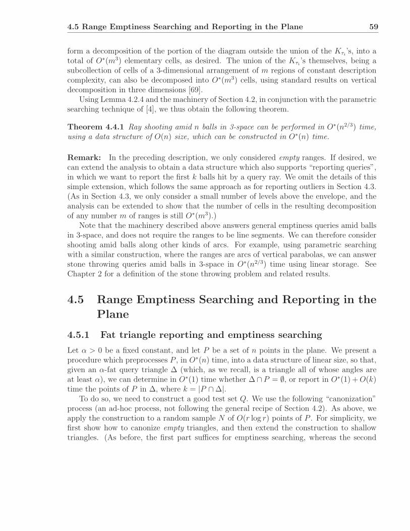
4.5 Range Emptiness Searching and Reporting in the Plane 59
form a decomposition of the portion of the diagram outside the union of the Kτi’s, into a
total of O∗(m3) elementary cells, as desired. The union of the Kτi’s themselves, being a
subcollection of cells of a 3-dimensional arrangement of m regions of constant descriptioncomplexity, can also be decomposed into O∗(m3) cells, using standard results on verticaldecomposition in three dimensions [69].
Using Lemma 4.2.4 and the machinery of Section 4.2, in conjunction with the parametricsearching technique of [4], we thus obtain the following theorem.
Theorem 4.4.1 Ray shooting amid n balls in 3-space can be performed in O∗(n2/3) time,using a data structure of O(n) size, which can be constructed in O∗(n) time.
Remark: In the preceding description, we only considered empty ranges. If desired, wecan extend the analysis to obtain a data structure which also supports “reporting queries”,in which we want to report the first k balls hit by a query ray. We omit the details of thissimple extension, which follows the same approach as for reporting outliers in Section 4.3.(As in Section 4.3, we only consider a small number of levels above the envelope, and theanalysis can be extended to show that the number of cells in the resulting decompositionof any number m of ranges is still O∗(m3).)
Note that the machinery described above answers general emptiness queries amid ballsin 3-space, and does not require the ranges to be line segments. We can therefore considershooting amid balls along other kinds of arcs. For example, using parametric searchingwith a similar construction, where the ranges are arcs of vertical parabolas, we can answerstone throwing queries amid balls in 3-space in O∗(n2/3) time using linear storage. SeeChapter 2 for a definition of the stone throwing problem and related results.
4.5 Range Emptiness Searching and Reporting in the
Plane
4.5.1 Fat triangle reporting and emptiness searching
Let α > 0 be a fixed constant, and let P be a set of n points in the plane. We present aprocedure which preprocesses P , in O∗(n) time, into a data structure of linear size, so that,given an α-fat query triangle ∆ (which, as we recall, is a triangle all of whose angles areat least α), we can determine in O∗(1) time whether ∆∩P = ∅, or report in O∗(1) + O(k)time the points of P in ∆, where k = |P ∩ ∆|.
To do so, we need to construct a good test set Q. We use the following “canonization”process (an ad-hoc process, not following the general recipe of Section 4.2). As above, weapply the construction to a random sample N of O(r log r) points of P . For simplicity, wefirst show how to canonize empty triangles, and then extend the construction to shallowtriangles. (As before, the first part suffices for emptiness searching, whereas the second
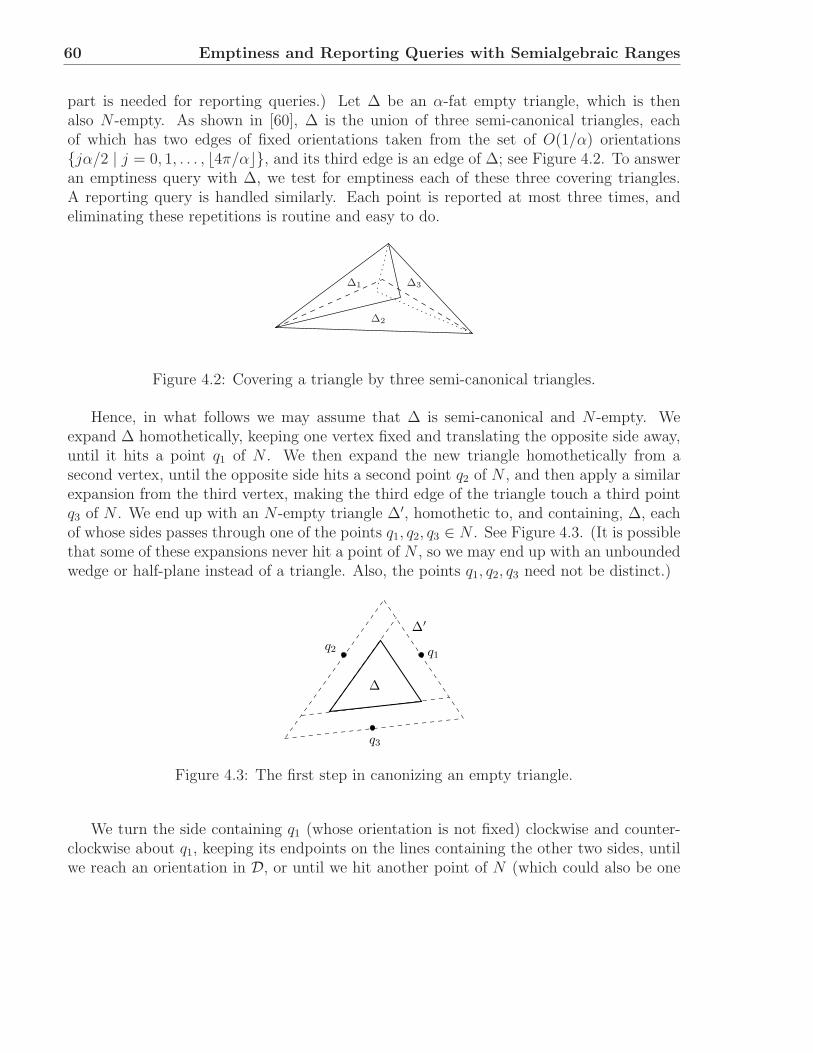
60 Emptiness and Reporting Queries with Semialgebraic Ranges
part is needed for reporting queries.) Let ∆ be an α-fat empty triangle, which is thenalso N -empty. As shown in [60], ∆ is the union of three semi-canonical triangles, eachof which has two edges of fixed orientations taken from the set of O(1/α) orientationsjα/2 | j = 0, 1, . . . , ⌊4π/α⌋, and its third edge is an edge of ∆; see Figure 4.2. To answeran emptiness query with ∆, we test for emptiness each of these three covering triangles.A reporting query is handled similarly. Each point is reported at most three times, andeliminating these repetitions is routine and easy to do.
∆1
∆2
∆3
Figure 4.2: Covering a triangle by three semi-canonical triangles.
Hence, in what follows we may assume that ∆ is semi-canonical and N -empty. Weexpand ∆ homothetically, keeping one vertex fixed and translating the opposite side away,until it hits a point q1 of N . We then expand the new triangle homothetically from asecond vertex, until the opposite side hits a second point q2 of N , and then apply a similarexpansion from the third vertex, making the third edge of the triangle touch a third pointq3 of N . We end up with an N -empty triangle ∆′, homothetic to, and containing, ∆, eachof whose sides passes through one of the points q1, q2, q3 ∈ N . See Figure 4.3. (It is possiblethat some of these expansions never hit a point of N , so we may end up with an unboundedwedge or half-plane instead of a triangle. Also, the points q1, q2, q3 need not be distinct.)
q3
∆
∆′
q1q2
Figure 4.3: The first step in canonizing an empty triangle.
We turn the side containing q1 (whose orientation is not fixed) clockwise and counter-clockwise about q1, keeping its endpoints on the lines containing the other two sides, untilwe reach an orientation in D, or until we hit another point of N (which could also be one

4.5 Range Emptiness Searching and Reporting in the Plane 61
of the points q2, q3), whichever comes first. Each of the new sides forms, with the two linescontaining the two other sides, a new (openly) N -empty (α/2)-fat triangle; the union ofthese two triangles covers ∆′. See Figure 4.4.
q1q2
q3
∆′
Figure 4.4: The second step in canonizing an empty triangle.
Each of these new triangles is (α/2)-fat, openly N -empty, has two sides at fixed ori-entations, each passing through a point of N , and a third side which either has a fixedorientation and passes through a point of N or passes through two points of N . Since|D| = O(1/α) = O(1), it follows that the overall number of these canonical covering tri-angles is O((r log r)4) = O∗(r4). (We omit the easy extensions of this step to handleunbounded wedges or half-planes, or the cases where the points qi, or some of the newlyencountered points, lie at vertices of the respective triangles.)
We take Q to be the collection of these canonical triangles, and argue that Q indeedsatisfies the properties of a good test set (with high probability): (a) Compactness: |Q| =O∗(r4), so its size is small. (b) Shallowness: With high probability, each range in Q is (n/r)-shallow (and, as usual, we assume that this property does indeed hold for our choice of N).(c) Containment: By construction, each (semi-canonical) α-fat empty triangle is containedin the union of at most six triangles in Q. (d) Efficiency: Being (α/2)-fat, the union of anym triangles in Q has complexity O(m log∗ m) (this is a very recent improvement over the“classical” O(m log log m) bound of [60]; see [43] and [13]). Hence the associated functionζ satisfies ζ(m) = O(m log∗ m), and ζ−1(r) = O( r
log∗ r). Combined with Lemma 4.2.4 and
the machinery of Section 4.2, we get the following recursion for the query time:
Q(n) ≤ D(r) + O(log∗ r)Q(n/r),
where D(r) bounds the time needed to find which of the O(r) cells of the partition arecrossed by ∆ and which are (fully) contained in ∆. Choosing r = O(1) and accepting abrute force solution with D(r) = O(r), we get the following theorem:
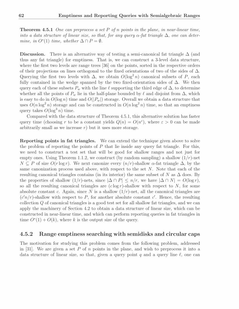
62 Emptiness and Reporting Queries with Semialgebraic Ranges
Theorem 4.5.1 One can preprocess a set P of n points in the plane, in near-linear time,into a data structure of linear size, so that, for any query α-fat triangle ∆, one can deter-mine, in O∗(1) time, whether ∆ ∩ P = ∅.
Discussion. There is an alternative way of testing a semi-canonical fat triangle ∆ (andthus any fat triangle) for emptiness. That is, we can construct a 3-level data structure,where the first two levels are range trees [36] on the points, sorted in the respective ordersof their projections on lines orthogonal to the fixed orientations of two of the sides of ∆.Querying the first two levels with ∆, we obtain O(log2 n) canonical subsets of P , eachfully contained in the wedge spanned by the two fixed-orientation sides of ∆. We thenquery each of these subsets Pw with the line ℓ supporting the third edge of ∆, to determinewhether all the points of Pw lie in the half-plane bounded by ℓ and disjoint from ∆, whichis easy to do in O(log n) time and O(|Pw|) storage. Overall we obtain a data structure thatuses O(n log2 n) storage and can be constructed in O(n log2 n) time, so that an emptinessquery takes O(log3 n) time.
Compared with the data structure of Theorem 4.5.1, this alternative solution has fasterquery time (choosing r to be a constant yields Q(n) = O(nε), where ε > 0 can be madearbitrarily small as we increase r) but it uses more storage.
Reporting points in fat triangles. We can extend the technique given above to solvethe problem of reporting the points of P that lie inside any query fat triangle. For this,we need to construct a test set that will be good for shallow ranges and not just forempty ones. Using Theorem 1.1.2, we construct (by random sampling) a shallow (1/r)-netN ⊆ P of size O(r log r). We next canonize every (n/r)-shallow α-fat triangle ∆, by thesame canonization process used above, with respect to the set N . Note that each of theresulting canonical triangles contains (in its interior) the same subset of N as ∆ does. Bythe properties of shallow (1/r)-nets, since |∆ ∩ P | ≤ n/r, we have |∆ ∩ N | = O(log r),so all the resulting canonical triangles are (c log r)-shallow with respect to N , for someabsolute constant c. Again, since N is a shallow (1/r)-net, all the canonical triangles are(c′n/r)-shallow with respect to P , for another absolute constant c′. Hence, the resultingcollection Q of canonical triangles is a good test set for all shallow fat triangles, and we canapply the machinery of Section 4.2 to obtain a data structure of linear size, which can beconstructed in near-linear time, and which can perform reporting queries in fat triangles intime O∗(1) + O(k), where k is the output size of the query.
4.5.2 Range emptiness searching with semidisks and circular caps
The motivation for studying this problem comes from the following problem, addressedin [31]. We are given a set P of n points in the plane, and wish to preprocess it into adata structure of linear size, so that, given a query point q and a query line ℓ, one can
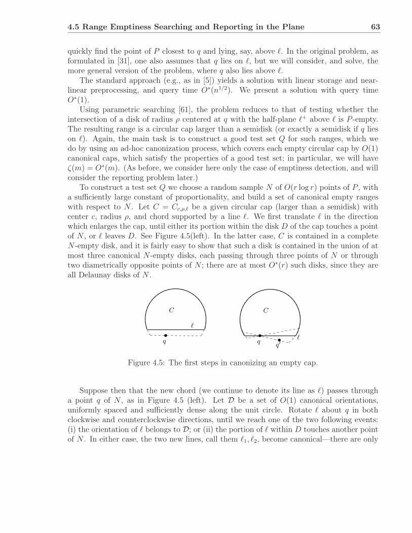
4.5 Range Emptiness Searching and Reporting in the Plane 63
quickly find the point of P closest to q and lying, say, above ℓ. In the original problem, asformulated in [31], one also assumes that q lies on ℓ, but we will consider, and solve, themore general version of the problem, where q also lies above ℓ.
The standard approach (e.g., as in [5]) yields a solution with linear storage and near-linear preprocessing, and query time O∗(n1/2). We present a solution with query timeO∗(1).
Using parametric searching [61], the problem reduces to that of testing whether theintersection of a disk of radius ρ centered at q with the half-plane ℓ+ above ℓ is P -empty.The resulting range is a circular cap larger than a semidisk (or exactly a semidisk if q lieson ℓ). Again, the main task is to construct a good test set Q for such ranges, which wedo by using an ad-hoc canonization process, which covers each empty circular cap by O(1)canonical caps, which satisfy the properties of a good test set; in particular, we will haveζ(m) = O∗(m). (As before, we consider here only the case of emptiness detection, and willconsider the reporting problem later.)
To construct a test set Q we choose a random sample N of O(r log r) points of P , witha sufficiently large constant of proportionality, and build a set of canonical empty rangeswith respect to N . Let C = Cc,ρ,ℓ be a given circular cap (larger than a semidisk) withcenter c, radius ρ, and chord supported by a line ℓ. We first translate ℓ in the directionwhich enlarges the cap, until either its portion within the disk D of the cap touches a pointof N , or ℓ leaves D. See Figure 4.5(left). In the latter case, C is contained in a completeN -empty disk, and it is fairly easy to show that such a disk is contained in the union of atmost three canonical N -empty disks, each passing through three points of N or throughtwo diametrically opposite points of N ; there are at most O∗(r) such disks, since they areall Delaunay disks of N .
q′
C
ℓ
q
C
qℓ
Figure 4.5: The first steps in canonizing an empty cap.
Suppose then that the new chord (we continue to denote its line as ℓ) passes througha point q of N , as in Figure 4.5 (left). Let D be a set of O(1) canonical orientations,uniformly spaced and sufficiently dense along the unit circle. Rotate ℓ about q in bothclockwise and counterclockwise directions, until we reach one of the two following events:(i) the orientation of ℓ belongs to D; or (ii) the portion of ℓ within D touches another pointof N . In either case, the two new lines, call them ℓ1, ℓ2, become canonical—there are only
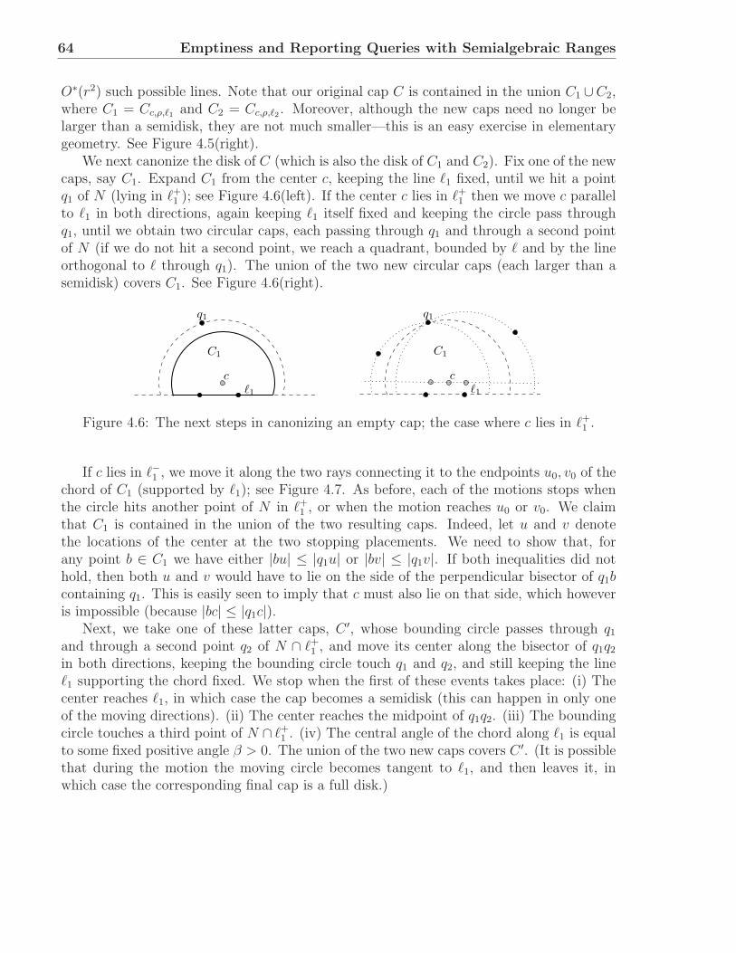
64 Emptiness and Reporting Queries with Semialgebraic Ranges
O∗(r2) such possible lines. Note that our original cap C is contained in the union C1 ∪C2,where C1 = Cc,ρ,ℓ1 and C2 = Cc,ρ,ℓ2 . Moreover, although the new caps need no longer belarger than a semidisk, they are not much smaller—this is an easy exercise in elementarygeometry. See Figure 4.5(right).
We next canonize the disk of C (which is also the disk of C1 and C2). Fix one of the newcaps, say C1. Expand C1 from the center c, keeping the line ℓ1 fixed, until we hit a pointq1 of N (lying in ℓ+
1 ); see Figure 4.6(left). If the center c lies in ℓ+1 then we move c parallel
to ℓ1 in both directions, again keeping ℓ1 itself fixed and keeping the circle pass throughq1, until we obtain two circular caps, each passing through q1 and through a second pointof N (if we do not hit a second point, we reach a quadrant, bounded by ℓ and by the lineorthogonal to ℓ through q1). The union of the two new circular caps (each larger than asemidisk) covers C1. See Figure 4.6(right).
q1
c
C1
q1
c
C1
ℓ1 ℓ1
Figure 4.6: The next steps in canonizing an empty cap; the case where c lies in ℓ+1 .
If c lies in ℓ−1 , we move it along the two rays connecting it to the endpoints u0, v0 of thechord of C1 (supported by ℓ1); see Figure 4.7. As before, each of the motions stops whenthe circle hits another point of N in ℓ+
1 , or when the motion reaches u0 or v0. We claimthat C1 is contained in the union of the two resulting caps. Indeed, let u and v denotethe locations of the center at the two stopping placements. We need to show that, forany point b ∈ C1 we have either |bu| ≤ |q1u| or |bv| ≤ |q1v|. If both inequalities did nothold, then both u and v would have to lie on the side of the perpendicular bisector of q1bcontaining q1. This is easily seen to imply that c must also lie on that side, which howeveris impossible (because |bc| ≤ |q1c|).
Next, we take one of these latter caps, C ′, whose bounding circle passes through q1
and through a second point q2 of N ∩ ℓ+1 , and move its center along the bisector of q1q2
in both directions, keeping the bounding circle touch q1 and q2, and still keeping the lineℓ1 supporting the chord fixed. We stop when the first of these events takes place: (i) Thecenter reaches ℓ1, in which case the cap becomes a semidisk (this can happen in only oneof the moving directions). (ii) The center reaches the midpoint of q1q2. (iii) The boundingcircle touches a third point of N ∩ ℓ+
1 . (iv) The central angle of the chord along ℓ1 is equalto some fixed positive angle β > 0. The union of the two new caps covers C ′. (It is possiblethat during the motion the moving circle becomes tangent to ℓ1, and then leaves it, inwhich case the corresponding final cap is a full disk.)
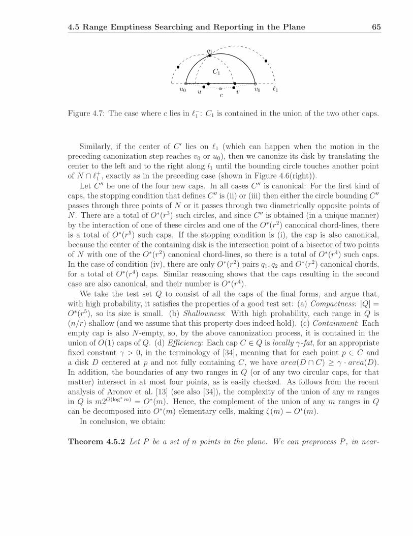
4.5 Range Emptiness Searching and Reporting in the Plane 65
q1
C1
cvuu0 v0 ℓ1
Figure 4.7: The case where c lies in ℓ−1 : C1 is contained in the union of the two other caps.
Similarly, if the center of C ′ lies on ℓ1 (which can happen when the motion in thepreceding canonization step reaches v0 or u0), then we canonize its disk by translating thecenter to the left and to the right along l1 until the bounding circle touches another pointof N ∩ ℓ+
1 , exactly as in the preceding case (shown in Figure 4.6(right)).
Let C ′′ be one of the four new caps. In all cases C ′′ is canonical: For the first kind ofcaps, the stopping condition that defines C ′′ is (ii) or (iii) then either the circle bounding C ′′
passes through three points of N or it passes through two diametrically opposite points ofN . There are a total of O∗(r3) such circles, and since C ′′ is obtained (in a unique manner)by the interaction of one of these circles and one of the O∗(r2) canonical chord-lines, thereis a total of O∗(r5) such caps. If the stopping condition is (i), the cap is also canonical,because the center of the containing disk is the intersection point of a bisector of two pointsof N with one of the O∗(r2) canonical chord-lines, so there is a total of O∗(r4) such caps.In the case of condition (iv), there are only O∗(r2) pairs q1, q2 and O∗(r2) canonical chords,for a total of O∗(r4) caps. Similar reasoning shows that the caps resulting in the secondcase are also canonical, and their number is O∗(r4).
We take the test set Q to consist of all the caps of the final forms, and argue that,with high probability, it satisfies the properties of a good test set: (a) Compactness: |Q| =O∗(r5), so its size is small. (b) Shallowness: With high probability, each range in Q is(n/r)-shallow (and we assume that this property does indeed hold). (c) Containment: Eachempty cap is also N -empty, so, by the above canonization process, it is contained in theunion of O(1) caps of Q. (d) Efficiency: Each cap C ∈ Q is locally γ-fat, for an appropriatefixed constant γ > 0, in the terminology of [34], meaning that for each point p ∈ C anda disk D centered at p and not fully containing C, we have area(D ∩ C) ≥ γ · area(D).In addition, the boundaries of any two ranges in Q (or of any two circular caps, for thatmatter) intersect in at most four points, as is easily checked. As follows from the recentanalysis of Aronov et al. [13] (see also [34]), the complexity of the union of any m rangesin Q is m2O(log∗ m) = O∗(m). Hence, the complement of the union of any m ranges in Qcan be decomposed into O∗(m) elementary cells, making ζ(m) = O∗(m).
In conclusion, we obtain:
Theorem 4.5.2 Let P be a set of n points in the plane. We can preprocess P , in near-
66 Emptiness and Reporting Queries with Semialgebraic Ranges
linear time, into a data structure of linear size, so that, for any query circular cap C, largerthan or equal to a semidisk, we can test whether C ∩ P is empty in O∗(1) time.
Combining Theorem 4.5.2 with parametric searching, we obtain:
Corollary 4.5.3 Let P be a set of n points in the plane. We can preprocess P , in near-linear time, into a data structure of linear size, so that, for any query half-plane ℓ+ andpoint q ∈ ℓ+, we can find, in O∗(1) time, the point in P ∩ ℓ+ nearest to q.
Remark. The machinery developed in this section also applies to smaller circular caps, aslong as they are not too small. Formally, if the central angle of each cap is at least somefixed constant α > 0, the same technique holds, so we can test emptiness of such ranges inO∗(1) time, using a data structure which requires O(n) storage and O∗(n) preprocessing.Thus Theorem 4.5.2 carries over to this scenario, but Corollary 4.5.3 does not, because wehave no control over the “fatness” of the cap, as the disk shrinks or expands, when thecenter of the disk lies in ℓ−, and once the canonical caps become too thin, the complexityof their union may become quadratic.
The technique described here can be used to answer queries that seek the farthest pointabove a line, where we want to preprocess a set P of n points, so that, given a line ℓ and apoint p on (or above) ℓ, we can find the point q ∈ P that lies above ℓ and is farthest fromp. Similarly to the problem of finding the farthest point from a convex shape in 3-space,studied in Section 4.3.1, the test set created here is a set of semidisks, each containingat least n − n/r points of P for some constant r > 0. The function ζ(r) we considerhere bounds the number of elementary cells in the decomposition of the intersection of rsemidisks. It is easy to verify that the complexity of the decomposition of the intersectionof r semidisks is O(λ4(r)). This immediately leads to a linear size data structure that cananswer queries for the farthest point above a line in O∗(1) time.
Reporting points in semidisks and circular caps. As in the case of fat triangles,we can extend the technique to answer efficiently range reporting queries in semidisks orin sufficiently large circular caps. We use the same canonization process, with respect to arandom sample N of size O(r log r) which is a shallow (1/r)-net, and argue, exactly as inthe case of fat triangles, that the resulting collection of canonical caps is a good test set forshallow semidisk or larger cap ranges. Applying the machinery of Section 4.2, we obtain adata structure of linear size, which can be constructed in near-linear time, and which canperform reporting queries in semidisks or larger caps, in time O∗(1) + O(k), where k is theoutput size of the query.
4.6 Conclusions 67
4.6 Conclusions
In this chapter we have presented a general approach to efficient range emptiness searchingwith semialgebraic ranges, and have applied it to several specific emptiness searching andray shooting problems. The present study resolves and overcomes the technical problemsencountered in our earlier study [71], and presents more applications of the technique.
Clearly, there are many other applications of the new machinery, and an obvious direc-tion for further research is to “dig them up”. In each such problem, the main step wouldbe to design a good test set, with associated function ζ(·) as small as possible, using eitherthe general recipe or an appropriate ad-hoc analysis. Many specific instances of this stepare likely to generate interesting (and often hard) combinatorial questions. For example,as already mentioned earlier, we still do not know whether the complement of the unionof n (congruent) cylinders in R
3 can be decomposed into O∗(n2) elementary cells. Thissubproblem arises in the design of a data structure for a set P on n points in R
3, whichsupports efficient queries where we specify a line ℓ and want to find the point of P nearestto ℓ.

68 Emptiness and Reporting Queries with Semialgebraic Ranges
Chapter 5
Approximate Semialgebraic RangeCounting
Only by counting could humans demonstrate their independence of computers.(The Hitchhiker’s Guide to the Galaxy)
Ford carried on counting quietly. This is about the most aggressive thing youcan do to a computer, the equivalent of going up to a human being and sayingBlood... blood... blood... blood...(The Hitchhiker’s Guide to the Galaxy)
5.1 Overview
Given a set P of n points in Rd, a set Γ of semialgebraic ranges of constant description
complexity, and a parameter ε > 0, the approximate range counting problem is to preprocessP into a data structure such that, for any query range γ ∈ Γ, we can efficiently computean approximate count tγ which satisfies
(1 − ε)|P ∩ γ| ≤ tγ ≤ (1 + ε)|P ∩ γ|.
As in Chapters 2 and 4, we only consider the case where the size of the data structure isto be (almost) linear, and the goal is to find solutions with small query time.
The problem has been studied in several recent papers [15, 16, 17, 51], for the specialcase where P is a set of points in R
d and Γ is the collection of half-spaces (bounded byhyperplanes). A variety of solutions, with near-linear storage, were derived; in all of them,the dependence of the query cost on n is close to n1−1/⌊d/2⌋, which, as reviewed in theintroduction, is roughly the same as the cost of half-space range emptiness queries, or theoverhead cost of half-space range reporting queries [57].
The fact that the approximate range counting problem is closely related to range empti-ness comes as no surprise, because, when P ∩ γ = ∅, the approximate count tγ must be 0,

70 Approximate Semialgebraic Range Counting
so range emptiness is a special case of approximate range counting. The goal is thereforeto derive solutions that are comparable, in their dependence on n, with those that solveemptiness (or reporting) queries. As just noted, this has been accomplished for the caseof half-spaces. In this chapter we extend this technique to the general semialgebraic case,exploiting the results that we have obtained in Chapter 4.
We present two solutions for this problem. The first solution, given in Section 5.2, plugsour algorithm for emptiness queries as a black box into the machinery of Aronov and Har-Peled [15], which effectively performs a binary search over the unknown size of the queryoutput. The second solution is based on another recent technique of Aronov and Sharir [17].Their technique, originally designed for half-space ranges, constructs a modified partitiontree for half-space emptiness or reporting, where some extra data is stored at each node ofthe tree. In Section 5.3 we modify their technique to handle general semialgebraic ranges.In Section 5.4 we consider a variant where each point p ∈ P has an associated weight w(p),so that, given a range γ and a parameter k > 1, we wish to report efficiently the k pointsin P ∩ γ that have the largest weights.
5.2 First Approach
The simplest solution is to adapt the technique of Aronov and Har-Peled [15], which usesa procedure for answering range emptiness queries as a “black box”. Specifically, supposewe have a data structure, D(P ′), for any set P ′ of n′ points, which can be constructedin T (n′) time, uses S(n′) storage, and can determine whether a query range γ ∈ Γ isP ′-empty in Q(n′) time. Using such a black box, Aronov and Har-Peled show how toconstruct an approximate range counting data structure for a set P of n input points
and a specified error parameter ε, using O((ελ−3 +
∑⌈1/ε⌉i=1 1/iλ−2)S(n) log n
)storage and
O((ελ−3 +
∑⌈1/ε⌉i=1 1/iλ−2)T (n) log n
)preprocessing, where λ ≥ 1 is some constant for which
S(n/r) = O(S(n)/rλ) and T (n/r) = O(T (n)/rλ), for any r > 1. Given a range γ ∈Γ, this structure returns, in O(ε−2Q(n) log n) time, an approximate count tγ, satisfying(1 − ε)|γ ∩ P | ≤ tγ ≤ |γ ∩ P |.
The intuition behind this approach is that a range γ, containing m points of P , isexpected to contain mr/n points in a random sample of P of size r, and most likely itcontains no points in a sample of size significantly smaller than n/m. The algorithm of [15]then guesses the value of m (up to a factor of 1 + ε), sets r to be an appropriate multipleof n/m, and draws many (specifically, O(ε−2 log n)) random samples of P of size r. If γ isempty (resp., nonempty) for many of the samples then, with high probability, the guess form is too large (resp., too small). When we cannot decide either way, we are at the correctvalue of m (up to a relative error of ε). The actual details of the search are somewhat morecontrived; see [15].
Plugging our emptiness data structures into the machinery of [15], we therefore obtain

5.3 Second Approach 71
the following results. In all these applications we can take λ = 1, because of the near-linearsize of our data structures, so, using the above bounds, the overall data structure requiresO(ε−2S(n) log n) storage and O(ε−2T (n) log n) preprocessing, where S(n) and T (n) are thestorage and preprocessing bounds for our data structures. In the bounds stated in thecorollaries, the O∗(·) notation refers to the dependence on n only.
Corollary 5.2.1 Let P be a set of n points in the plane, and let α, ε be given positiveparameters. Then we can preprocess P into a data structure of size O(ε−2n log n), in timeO∗(ε−2n), such that, for any α-fat query triangle ∆, we can compute, in O∗(ε−2) time, anapproximate count t∆ satisfying (1 − ε)|∆ ∩ P | ≤ t∆ ≤ |∆ ∩ P |.
Corollary 5.2.2 Let P be a set of n points in the plane, and let ε be a given positiveparameter. Then we can preprocess P into a data structure of size O(ε−2n log n), in timeO∗(ε−2n), such that, for any line ℓ, a point p on ℓ or above ℓ, and distance d, we cancompute, in O∗(ε−2) time, an approximate count tℓ,p,d of the exact number Nℓ,p,d of the pointsof P which lie above ℓ and at distance at most d from p, so that (1−ε)Nℓ,p,d ≤ tℓ,p,d ≤ Nℓ,p,d.
Corollary 5.2.3 Let P be a set of n points in R3, Γ a collection of convex semialgebraic
ranges of constant description complexity, and ε a given positive parameter. Then we canpreprocess P into a data structure of size O(ε−2n log n), in time O∗(ε−2n), such that, forany query range γ ∈ Γ, we can compute, in O∗(ε−2n1/2) time, an approximate count tγ ofthe number of points of P outside γ, satisfying (1 − ε)|γc ∩ P | ≤ tγ ≤ |γc ∩ P |.
Corollary 5.2.4 Let B be a set of n balls in R3, and let ε be a given positive parameter.
Then we can preprocess B into a data structure of size O(ε−2n log n), in time O∗(ε−2n), suchthat, for any query ray or segment ρ, we can compute, in O∗(ε−2n2/3) time, an approximatecount tρ of the exact number Nρ of the balls of B intersected by ρ, satisfying (1 − ε)Nρ ≤tρ ≤ Nρ.
5.3 Second Approach
Another approach to approximate range counting has been presented in [16, 17], in which,rather than using a range emptiness searching procedure as a black box, one modifies thepartition tree of the range emptiness data structure, and augments each of its inner nodeswith a relative (p, ε)-approximation set (as reviewed in Section 1.1.9). These sets are thenused to obtain the approximate count of any “heavy” range that visits that node (see belowfor details). As we show in this section, this approach too can be adapted to yield efficientapproximate range counting algorithms for semialgebraic ranges, with a slightly improveddependence of their performance on ε (as in the case of halfspaces, studied in [16, 17]).
Let P be a given set of n points in Rd, and let ε > 0 be a given parameter. Following the
scheme of [17], we build a partition tree T , where each node v represents a subset Pv ⊆ P
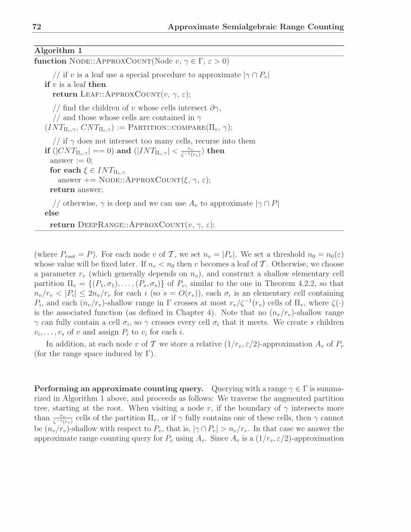
72 Approximate Semialgebraic Range Counting
Algorithm 1
function Node::ApproxCount(Node v, γ ∈ Γ, ε > 0)
// if v is a leaf use a special procedure to approximate |γ ∩ Pv|if v is a leaf then
return Leaf::ApproxCount(v, γ, ε);
// find the children of v whose cells intersect ∂γ,// and those whose cells are contained in γ
(INTΠv ,γ, CNTΠv ,γ) := Partition::compare(Πv, γ);
// if γ does not intersect too many cells, recurse into themif (|CNTΠv ,γ| == 0) and (|INTΠv,γ| < rv
ζ−1(rv)) then
answer := 0;for each ξ ∈ INTΠv ,γ
answer += Node::ApproxCount(ξ, γ, ε);return answer;
// otherwise, γ is deep and we can use Av to approximate |γ ∩ P |else
return DeepRange::ApproxCount(v, γ, ε);
(where Proot = P ). For each node v of T , we set nv = |Pv|. We set a threshold n0 = n0(ε)whose value will be fixed later. If nv < n0 then v becomes a leaf of T . Otherwise, we choosea parameter rv (which generally depends on nv), and construct a shallow elementary cellpartition Πv = (P1, σ1), . . . , (Ps, σs) of Pv, similar to the one in Theorem 4.2.2, so thatnv/rv < |Pi| ≤ 2nv/rv for each i (so s = O(rv)), each σi is an elementary cell containingPi, and each (nv/rv)-shallow range in Γ crosses at most rv/ζ
−1(rv) cells of Πv, where ζ(·)is the associated function (as defined in Chapter 4). Note that no (nv/rv)-shallow rangeγ can fully contain a cell σi, so γ crosses every cell σi that it meets. We create s childrenvi, . . . , vs of v and assign Pi to vi for each i.
In addition, at each node v of T we store a relative (1/rv, ε/2)-approximation Av of Pv
(for the range space induced by Γ).
Performing an approximate counting query. Querying with a range γ ∈ Γ is summa-rized in Algorithm 1 above, and proceeds as follows: We traverse the augmented partitiontree, starting at the root. When visiting a node v, if the boundary of γ intersects morethan rv
ζ−1(rv)cells of the partition Πv, or if γ fully contains one of these cells, then γ cannot
be (nv/rv)-shallow with respect to Pv, that is, |γ ∩Pv| > nv/rv. In that case we answer theapproximate range counting query for Pv using Av. Since Av is a (1/rv, ε/2)-approximation
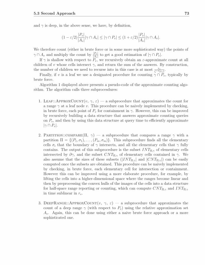
5.3 Second Approach 73
and γ is deep, in the above sense, we have, by definition,
(1 − ε/2)|Pv||Av|
|γ ∩ Av| ≤ |γ ∩ Pv| ≤ (1 + ε/2)|Pv||Av|
|γ ∩ Av|.
We therefore count (either in brute force or in some more sophisticated way) the points of
γ ∩ Av and multiply the count by |Pv ||Av | to get a good estimation of |γ ∩ Pv|.
If γ is shallow with respect to Pv, we recursively obtain an ε-approximate count at allchildren of v whose cells intersect γ, and return the sum of the answers. By construction,the number of children we need to recurse into in this case is at most rv
ζ−1(rv).
Finally, if v is a leaf we use a designated procedure for counting γ ∩ Pv, typically bybrute force.
Algorithm 1 displayed above presents a pseudo-code of the approximate counting algo-rithm. The algorithm calls three subprocesdures:
1. Leaf::ApproxCount(v, γ, ε) — a subprocedure that approximates the count fora range γ at a leaf node v. This procedure can be naively implemented by checking,in brute force, each point of Pv for containment in γ. However, this can be improvedby recursively building a data structure that answers approximate counting querieson Pv, and then by using this data structure at query time to efficiently approximate|γ ∩ Pv|.
2. Partition::compare(Π, γ) — a subprocedure that compares a range γ with apartition Π = (P1, σ1), . . . , (Pm, σm). This subprocedure finds all the elementarycells σi that the boundary of γ intersects, and all the elementary cells that γ fullycontains. The output of this subprocedure is the subset INTΠ,γ of elementary cellsintersected by ∂γ, and the subset CNTΠ,γ of elementary cells contained in γ. Wealso assume that the sizes of these subsets (|INTΠ,γ| and |CNTΠ,γ|) can be easilycomputed once the subsets are obtained. This procedure can be naively implementedby checking, in brute force, each elementary cell for intersection or containment.However this can be improved using a more elaborate procedure, for example, bylifting the cells into a higher-dimensional space where the ranges become linear andthen by preprocessing the convex hulls of the images of the cells into a data structurefor half-space range reporting or counting, which can compute CNTΠ,γ and INTΠ,γ
in time sublinear in rv.
3. DeepRange::ApproxCount(v, γ, ε) — a subprocedure that approximates thecount of a deep range γ (with respect to Pv) using the relative approximation setAv. Again, this can be done using either a naive brute force approach or a moresophisticated one.

74 Approximate Semialgebraic Range Counting
5.3.1 Choosing the parameters
Choosing rv. We choose rv = nv
(ζ−1(nv))α′ , for some 1 < α′ < log(nv/4)log ζ−1(nv)
. The concrete
value of α′ will be discussed later. Typically, ζ(m) = Θ(mδ) for some constant δ ≥ 1, so,
for example, this restricts our choice to rv < n1/2v for approximating the number of points
outside a query cylinder in 3-space, or rv < n3/4v for approximating the number of balls a
query segment intersects in 3-space. The cases of estimating the number of points containedin a fat triangle, or the number of points contained in a semi-disk are especially interestingbecause in those cases ζ(nv) = Θ(nvpolylog(nv)), and our choice of rv is therefore restrictedby rv < polylog(nv).
Choosing the size of Av. We set Av to be a random sample of size crv
ε2 log rv (for anappropriate constant c > 0), which is a relative (1/rv, ε/2)-approximation with proba-bility at least 1 − 1/rb
v, where b = b(c) is linear in c. For technical reasons that arisein the analysis of the storage requirements we need to restrict the size of Av. Intu-itively we need Av to be small enough relatively to Pv. More specifically, we will requirethat |Av| = crv
ε2 log rv ≤ nv
k log3 log nv, for some constant k that will be specified later. By
the choice of rv we need (ζ−1(nv))α′ ≥ ck log3 log nv
ε2 log nv
ζ−1(nv)α′ which holds if we choose
nv ≥ ζ
((c′
ε2 log3 (log nv) log nv
ζ−1(nv)α′
)1/α′)
for an appropriate multiple c′ of c. We thus set
n0 = n0(ε) = ζ
((c′
ε2log3
(log
1
ε
)log
1
ε
)α′)
,
and enforce this lower bound on nv by declaring a node to be a leaf if it has at most n0
points, and continuing recursively to build the tree if it has more than n0 points.
5.3.2 Analysis of query-time, storage and preprocessing
Let Qleaf (n, ε), Qcomp(m) and Qdeep(n, ε) be the query time of the three respective proce-duresLeaf::ApproxCount, Partition::compare and DeepRange::ApproxCount, whererv/2 ≤ m ≤ rv is the number of elementary cells in the partition Πv, n = |Pv| is (withslight abuse of notation) the number of points associated with the current node, and εis the approximation parameter. Similarly let Tleaf (n, ε), Sleaf (n, ε) (Tcomp(m), Scomp(m),Tdeep(n, ε), Sdeep(n, ε)) be the preprocessing time and storage required by Leaf::ApproxCount(Partition::compare, DeepRange::ApproxCount). Also, let Tpart(n, ε) be the timeneeded to construct the partition at a node v. Similarly to the analysis in [17], we obtainthe following recurrences for the query time Q(n, ε), preprocessing time T (n, ε) and storageS(n, ε) of our data structure; here r = rv is the partitioning parameter used at v.
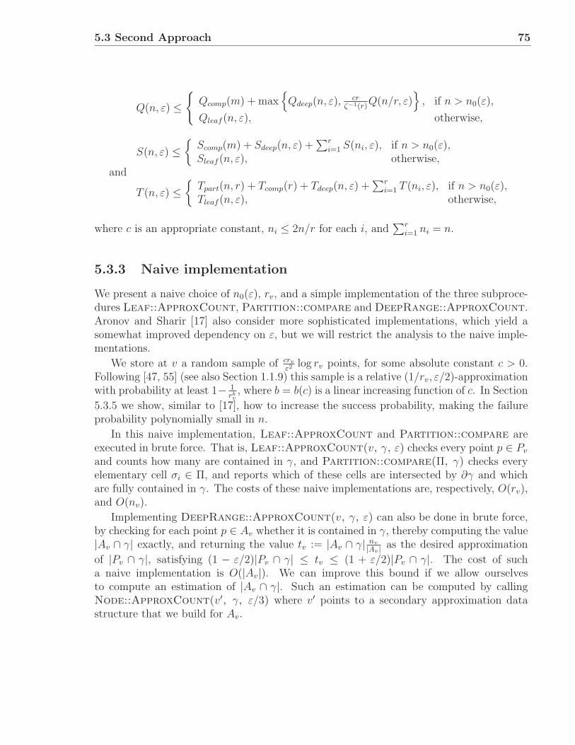
5.3 Second Approach 75
Q(n, ε) ≤
Qcomp(m) + max
Qdeep(n, ε), crζ−1(r)
Q(n/r, ε)
, if n > n0(ε),
Qleaf (n, ε), otherwise,
S(n, ε) ≤
Scomp(m) + Sdeep(n, ε) +∑r
i=1 S(ni, ε), if n > n0(ε),Sleaf (n, ε), otherwise,
and
T (n, ε) ≤
Tpart(n, r) + Tcomp(r) + Tdeep(n, ε) +∑r
i=1 T (ni, ε), if n > n0(ε),Tleaf (n, ε), otherwise,
where c is an appropriate constant, ni ≤ 2n/r for each i, and∑r
i=1 ni = n.
5.3.3 Naive implementation
We present a naive choice of n0(ε), rv, and a simple implementation of the three subproce-dures Leaf::ApproxCount, Partition::compare and DeepRange::ApproxCount.Aronov and Sharir [17] also consider more sophisticated implementations, which yield asomewhat improved dependency on ε, but we will restrict the analysis to the naive imple-mentations.
We store at v a random sample of crv
ε2 log rv points, for some absolute constant c > 0.Following [47, 55] (see also Section 1.1.9) this sample is a relative (1/rv, ε/2)-approximationwith probability at least 1− 1
rbv, where b = b(c) is a linear increasing function of c. In Section
5.3.5 we show, similar to [17], how to increase the success probability, making the failureprobability polynomially small in n.
In this naive implementation, Leaf::ApproxCount and Partition::compare areexecuted in brute force. That is, Leaf::ApproxCount(v, γ, ε) checks every point p ∈ Pv
and counts how many are contained in γ, and Partition::compare(Π, γ) checks everyelementary cell σi ∈ Π, and reports which of these cells are intersected by ∂γ and whichare fully contained in γ. The costs of these naive implementations are, respectively, O(rv),and O(nv).
Implementing DeepRange::ApproxCount(v, γ, ε) can also be done in brute force,by checking for each point p ∈ Av whether it is contained in γ, thereby computing the value|Av ∩ γ| exactly, and returning the value tv := |Av ∩ γ| nv
|Av | as the desired approximation
of |Pv ∩ γ|, satisfying (1 − ε/2)|Pv ∩ γ| ≤ tv ≤ (1 + ε/2)|Pv ∩ γ|. The cost of sucha naive implementation is O(|Av|). We can improve this bound if we allow ourselvesto compute an estimation of |Av ∩ γ|. Such an estimation can be computed by callingNode::ApproxCount(v′, γ, ε/3) where v′ points to a secondary approximation datastructure that we build for Av.
76 Approximate Semialgebraic Range Counting
From the properties of relative (1/rv, ε/2)-approximation we have
(1 − ε
2)|Pv ∩ γ| |Av|
|Pv|≤ |Av ∩ γ| ≤ (1 +
ε
2)|Pv ∩ γ| |Av|
|Pv|.
The output tγ of Node::ApproxCount(v′, γ, ε/3) satisfies
(1 − ε
3)|Av ∩ γ| ≤ tγ ≤ (1 +
ε
3)|Av ∩ γ|,
and therefore, for ε < 1, the following holds:
(1−ε)|Pv∩γ| |Av||Pv|
≤ (1−ε
2)(1−ε
3)|Pv∩γ| |Av|
|Pv|≤ tγ ≤ (1+
ε
2)(1+
ε
3)|Pv∩γ| |Av|
|Pv|≤ (1+ε)|Pv∩γ| |Av|
|Pv|.
Recall that we have set
n0(ε) = ζ
((c′
ε2log3
(log
1
ε
)log
1
ε
)1/α′)
.
Our goal is to make the query time satisfy Q(n, ε) ≤ F (ε) nζ−1(n)
logβ n, for some absolute
constant parameter β and function F (ε). In particular we want this bound to hold for leafnodes as well as deep nodes. For a leaf node we have Qleaf (n, ε) = O(n) so we require
n0(ε) ≤ c′′F (ε) n0(ε)ζ−1(n0(ε))
logβ n0(ε), where c′′ ≥ 1 is some constant. Clearly this holds when
n0(ε) = F (ε) n0(ε)ζ−1(n0(ε))
. We therefore put
F (ε) = ζ−1(n0(ε)) = ζ−1
(ζ
((c′
ε2log3
(log
1
ε
)log
1
ε
)1/α′))
=
(c′
ε2log3
(log
1
ε
)log
1
ε
)1/α′
.
Recall that α′ > 1 is chosen such that (ζ−1(n))α′< n. If ζ(n) = O(nδ), this means that
1 < α′ < δ, and F (ε) is approximately of the form 1/εγ , where γ satisfies 2/δ < γ < 2.Note that γ approaches its upper (resp., lower) bound as α′ approaches 1 (resp., δ). Ifζ(n) = O(n · polylog(n)) then α′ must be chosen close to 1 and so F (ε) is approximatelyof the form 1/ε2.
Query time. Once α′ is fixed, the recurrence for Q(n, ε) becomes:
Q(n, ε) ≤
O(
n(ζ−1(n))α′
)+ max
Q
(n
k log3(log n), ε
3
), µ
(n
(ζ−1(n))α′
)Q(2(ζ−1(n))α′
, ε)
, if n > n0(ε)
O(n), otherwise,,

5.3 Second Approach 77
where µ(r) is the maximum number of elementary cells a shallow range crosses. That is,
µ(r) = O
(r
ζ−1(r)
)= O
n(ζ−1(n))α′
ζ−1(
n(ζ−1(n))α′
)
.
We show in Section 5.3.4 that the recurrence solves to Q(n, ε) ≤ F (ε) nζ−1(n)
logβ n, for
an appropriate choice of β = β(α′).
Storage. The storage bound S(n, ε) satisfies the recurrence:
S(n, ε) ≤
O(
n(ζ−1(n))α′
)+ S
(n
k log3(log n), ε
3
)+
∑n/(ζ−1(n))α′
i=1 S(ni, ε), if n > n0(ε)
O(n), otherwise.,
where ni ≤ 2(ζ−1(n))α′for each i, and
∑n/(ζ−1(n))α′
i=1 ni = n.We show in section 5.3.4 that the recurrence solves to S(n) = O(n), with a constant
that is independent of ε. As will follow from the analysis, the factor log3 log n can bereplaced by any factor of the form log2+δ(log n), for any positive constant δ.
Preprocessing. In this naive implementation, Tcomp(k) = O(k) and Tleaf (n, ε) = O(n).For Tpart(n, r) we use the bounds in Chapter 4, namely, Tpart(n, r) = O(n1+δ), for anyδ > 0. The resulting recurrence for T (n, ε) is thus:
T (n, ε) ≤
O(n1+δ) + T(
nk log3(log n)
, ε3
)+
∑n/(ζ−1(n))α′
i=1 T (ni, ε), if n > n0(ε)
O(n), otherwise.,
where ni ≤ 2(ζ−1(n))α′for each i, and
∑n/(ζ−1(n))α′
i=1 ni = n, and we choose the O(n1+δ)version if α′ > α′
0 and the O(n log n) version otherwise. It is straightforward to verify thatthe solution of this recurrence is
T (n, ε) = O(n1+δ),
for any δ > 0. Here too the constants of proportionality are independent of ε. We summa-rize these results in the following theorem.
Theorem 5.3.1 Given a family Γ of semialgebraic ranges of constant description com-plexity, we can preprocess a set P of n points in R
d, with a pre-specified error parameter0 < ε < 1, into a data structure of size O(n), independent of ε, so that, with high probabil-ity, for any query range γ ∈ Γ, we can obtain a relative ε-approximate count of γ ∩ P , in
78 Approximate Semialgebraic Range Counting
time O(ε−α n
ζ−1(n)logβ n
), where α can be chosen anywhere in
(2 logn
nζ−1(n)
, 2), and β is
a constant that depends on α.The data structure can be constructed deterministically, except for the random samplings
that produce the various relative approximations. The (worst-case) preprocessing cost isO(n1+δ), for any δ > 0.
5.3.4 Solving the recurrences
In this section we show that the recurrences mentioned in the earlier section yield indeedthe bounds asserted above.
Analysis of query time. We want to show that the recurrence
Q(n, ε) ≤
O(
n(ζ−1(n))α′
)+ max
Q
(n
k log3(log n), ε
3
), µ
(n
(ζ−1(n))α′
)Q(2(ζ−1(n))α′
, ε)
, if n > n0(ε)
O(n), otherwise.
solves to Q(n, ε) ≤ F (ε) nζ−1(n)
logβ n, with F (ε) = ζ−1(n0(ε)) =(
c′
ε2 log3(log 1
ε
)log 1
ε
)1/α′
.
We prove this by induction on n. For n ≤ n0(ε) we need to show that F (ε) nζ−1(n)
logβ n ≥O(n) Which can be easily seen to be true since F (ε) n
ζ−1(n)logβ n = ζ−1(n0(ε))
nζ−1(n)
logβ n0(ε),
and ζ−1(n0(ε))ζ−1(n)
≥ 1. For carrying out the induction step for larger values of n we need toshow that
c1n(ζ−1(n))α′ + max
F
(ε3
) nk log3(log n)
ζ−1“
nk log3(log n)
” logβ nk log3(log n)
,
c2
n
(ζ−1(n))α′
ζ−1
„
n
(ζ−1(n))α′
«F (ε) 2(ζ−1(n))α′
ζ−1(2(ζ−1(n))α′)logβ(2(ζ−1(n))α′
)
≤ F (ε) n
ζ−1(n)logβ n
for appropriate constants c1, c2. If we calibrate the constant in the definition of F (ε), sothat F (ε) is always at least 2c1, then
c1n
(ζ−1(n))α′ ≤ c1n
ζ−1(n)≤ 1
2F (ε)
n
ζ−1(n)≤ 1
2F (ε)
n
ζ−1(n)logβ n.
Clearly,
nk log3(log n)
ζ−1(
nk log3(log n)
) logβ n
k log3(log n)≤
nk log3(log n)
ζ−1(
nk log3(log n)
) logβ n ≤ n
ζ−1(n)
ζ−1(k log3(log n))
k log3(log n)logβ n,
5.3 Second Approach 79
where the last inequality coming from our assumption that ζ(·) is well behaved, in the sensethat ζ(ab) ≤ ζ(a)ζ(b) for a, b ≥ 1. Also, under the same assumption,
n(ζ−1(n))α′
ζ−1(
n(ζ−1(n))α′
) · 2(ζ−1(n))α′
ζ−1(2(ζ−1(n))α′)≤ 2n
ζ−1(2n)≤ 2n
ζ−1(n),
and(
log(2(ζ−1(n)α′))
log n
)β
=
(1 + α′ log ζ−1(n)
log n
)β
=
(1
log n+ α′ logn ζ−1(n)
)β
.
Putting it all together, it suffices to show that
1
2+ max
F ( ε
3)
F (ε)
ζ−1(k log3(log n)
)
k log3(log n),
(1
log n+ α′ logn ζ−1(n)
)β
≤ 1.
An appropriate choice of α′ and n0(ε) guarentees that the expression in the rightmostparethesis is strictly smaller than 1. This, and the way F (ε) is defined, imply the desiredinequality if β and k are chosen large enough.
Note the trade-off between β and F (ε). We can make F (ε) asymptotically smaller ifwe increase α′ and consequently increase β. (The bound on the cost of a query can thusbe optimized, for given values of n and ε.)
Analysis of storage. We want to show that the solution of the recurrence
S(n, ε) ≤
O(
n(ζ−1(n))α′
)+ S
(n
k log3(log n), ε
3
)+
∑n/(ζ−1(n))α′
i=1 S(ni, ε), if n > n0(ε)
O(n), otherwise,
is linear in n, where ni ≤ 2(ζ−1(n))α′for each i and
∑n/(ζ−1(n))α′
i=1 ni = n.We first show that S(n) ≤ Dn log log n, where D is a constant that does not depend
on ε. We prove this by induction on n. Clearly it holds for n ≤ n0(ε) for an appropriatechoice of D (independent of ε). For larger values of n, we need to show that
c2n
(ζ−1(n))α′ +Dn
k log3(log n)log log
(n
k log3(log n)
)+
n/(ζ−1(n))α′
∑
i=1
Dni log log(2(ζ−1(n))α′
) ≤ Dn log log n,
for an appropriate constant c2. In the first term we use n(ζ−1(n))α′ < n; in the second term we
use log log(
nk log3(log n)
)< log log n; and in the third term we use
∑ni = n. It is therefore
sufficient to prove that
80 Approximate Semialgebraic Range Counting
c2
D log log n+
1
k log3(log n)+
log log(2n (ζ−1(n))α′
n
)
log log n≤ 1.
By our choice of α′, n(ζ−1(n))α′ > 4, and so
log log(2n (ζ−1(n))α′
n
)
log log n≤
log log
(n
((ζ−1(n))α′
n
) 12
)
log log n=
log(log n − 1
2log n
(ζ−1(n))α′
)
log log n=
log log n + log(1 − 1
2logn
n(ζ−1(n))α′
)
log log n.
It therefore remains to show that
c2
D log log n+
1
k log3(log n)+
log(1 − 1
2logn
n(ζ−1(n))α′
)
log log n≤ 0.
Recall that ζ(r) = O(rδ), for some δ that depends on the “complexity” of the ranges.In this case, the inequality becomes
c2
D+
1
k log2(log n)+
log(
12
(1 + α′
δ
))
log log n≤ 0,
which holds if we choose, say, α′ < ( 222/k − 1)δ, and D > 2c2k. (Again, we have a trade-
off: to reduce F (ε) asymptotically, we have to choose bigger α′, so k has to be chosenlarger, which causes the constant of proportionality in the storage bound to increase.)For certain classes of ranges we have ζ(r) = O(r · polylog(r)) < rq, for any q > 0. Insuch cases we fix q to be some constant and the bound is established trivially. In bothcases the argument that S(n, ε) < D log log n holds. Using this for n = |A| we get thatS(|A|, ε
3) ≤ Dn log log n
k log3(log n)= O( n
log2(log n)). Since O( n
log2(log n)) > O( n
ζ−1(n)) (recall that ζ−1(n) is
at most nq for some q < 1), we can replace the first two terms in the recurrence and obtain:
S(n) ≤
D′nlog2(log n)
+∑n/(ζ−1(n))α′
i=1 S(ni), if n > n0(ε),
D′n, otherwise,
for some absolute constant D′, with constraints on the ni as mentioned earlier.Aronov et al. showed in [17] that when ζ−1(n) = nδ, for some 0 < δ < 1, this recurrence
solves to S(n) = O(n), with the constant of proportionality independent of ε. We repeattheir analysis for general ζ−1(n). We unwind the recurrence as follows: When expandinga node v of the tree and forming its children, each child w satisfies, by construction,
5.3 Second Approach 81
(ζ−1(nv))α′ ≤ nw ≤ 2(ζ−1(nv))
α′ ≤ √nv(ζ
−1(nv))α′/2. The last inequality is true because,
by our choice of α′, we have nζ−1(n)α′ > 4. We say that a node v lies at a level j if
(1
2+
α′
2logn
(ζ−1(n)
))j+1
< logn nv ≤(
1
2+
α′
2logn
(ζ−1(n)
))j
,
or, in other words,
n
“
12+α′
2logn(ζ−1(n))
”j+1
< nv ≤ n
“
12+α′
2logn(ζ−1(n))
”j
.
Thus the root lies at level 0, and the maximum level is O(log log n). Also, no two nodeson a common path have the same level, so the sum of the sizes nv, over all nodes v of afixed level, is at most n. Hence, the sum of the overhead terms of all nodes at level j is atmost:
D′n
log2 log n( 12+α′
2logn(ζ−1(n)))
j+1 =D′n
log2((
12
+ α′
2logn (ζ−1(n))
)j+1log n
) =
D′n(log log n + (j + 1) log(1
2+ α′
2logn ζ−1(n)
)2 .
The sum of the amounts of storage S(nw) at the leaves w of the tree is clearly at most D′n.Hence, the overall storage requirements is at most
D′n +∑
j≥0
D′n(log log n + (j + 1) log(1
2+ α′
2logn ζ−1(n)
)2 .
The smallest value of any denominator is attained at the parents of the leaves w, and is atleast (log log n0(ε))
2, because logn(ζ−1(n))α′< 1. This implies (e.g., by replacing the sum
by an integral) that the sum can be bounded by O(n/ log log n0(ε)), which by the choiceof n0(ε), is O(n/ log log 1
ε) = O(n), if ε < 1 is chosen sufficiently small.
5.3.5 Ensuring high probability
So far we have assumed that for each node v, a relative (1/rv, ε/2)-approximation of arequired size can be constructed efficiently. A deterministic process that constructs such arelative approximation is fairly complicated; see [21]. Another way to construct a relative(1/rv, ε/2)-approximation is by random sampling (see Theorems 1.1.1 and 1.1.2). Althoughthis is much simpler, one still needs to verify that the points that were drawn indeed form arelative approximation with the appropriate parameters. In [17], Aronov and Sharir arguethat just drawing points (without any verification) still ensures high success probability.For the sake of completeness, we repeat their argument for the case of semialgebraic ranges.
82 Approximate Semialgebraic Range Counting
The implementation we suggested draws at each node v a random sample of size crv
ε2 log rv
and makes it the approximation set (without any verification). It is difficult to guaranteehigh success probability, because, as follows from Theorem 1.1.2, the failure probability ofsuch a sample at a node v is only O(1/rb
v), for some constant b that depends on c. For nodesv that are deep in the tree, rv is small, and the guarenteed success probability becomessmaller, approaching constant probability as we get closer to the leaves. Since the numberof distinct ranges is polynomial in n, bounding the overall failure probability via a naiveprobability union bound does not keep the overall failure probability small. Alternatively,increasing the sample size by a factor of log n would guarantee low failure probability, butthis might affect the algorithm performance.
Nevertheless, we argue that drawing random samples at each node (with some additionalsimple mechanisms) does indeed guarantee high success probability. The intuition is thatwe can think of all the elements of all approximation sets at all the nodes a query reachesas one approximation set, with elements coming from a node v appearing with weight (ormultiplicity) nv/rv. Another way to look at it is as a sequence of independent Bernoullitrials, with an appropriate weighted sum of their corresponding indicator variables beingthe approximate count that the algorithm produces. This implies that the errors that theindividual relative approximation sets incur tend to cancel each other out, leading to anoverall error that is much smaller than the sum of the individual errors.
In more detail, the analysis proceeds as follows. We consider a fixed range γ, andbound the probability that the query with γ fails to produce the desired ε-approximatecount. Consider the set V = V (i) of all nodes v that satisfy (i) n/2i < nv < n/2i−1, forsome fixed “level” i ≥ 1, (ii) v is reached by the query with γ, and (iii) γ intersects too manychildren of v (and therefore it is deep with respect to Pv), so Av is used to approximate|γ ∩ Pv|. For each of these nodes v, we can think of the relative-error approximation Av asa random sample, where each point of Pv is chosen independently with probability
pv =cvrv
ε2 log rv
nv
,
where cv is the constant in the bound of [47, 55] (see Theorem 1.1.2), which we adjust at v,multiplying it by at most a constant factor to ensure that the probabilities pv are all equalfor nodes v at the same level; we denote this common value by p(i), for nodes at level i. Ateach node v we approximate |γ ∩Av| by some count Aγ, and add Aγ ·nv/|Av| to the globalcount. Recall that Av is a relative (1/rv, ε/2)-approximation, and that Aγ is computed byrecursively calling ApproxCount with ε/3 as the error parameter. We can therefore treatthat Aγ as if it is the actual count of Av ∩ γ, without affecting the asymptotic bounds. Tofit into the new model, we slightly modify this step, and instead we add to the global count
|γ ∩ Av| · nv
E|Av|=
|γ ∩ Av|pv
=|γ ∩ Av|
p(i).
5.3 Second Approach 83
Hence, the overall count that the approximations yield at a fixed level i is 1p(i) ·
∑v∈V |γ ∩
Av| = 1p(i) · |γ∩A|, where A =
⋃v∈V Av. Under the above assumptions, we can treat |γ∩A|
as the sum of independent indicator variables Ix, for x ∈ γ ∩ ⋃v∈V Pv, where Ix = 1 if x is
chosen in the respective Av. The expected value of∑
x∈γ∩S
v∈V PvIx is
µ = E|γ ∩ A| = p(i) ·∑
v∈V
|γ ∩ Pv| =∑
v∈V
cvrv
ε2 log rv
nv
|γ ∩ Pv|.
Note that since γ is deep at each of the nodes v, by assumption, we have, |γ ∩ Pv| ≥ nv/rv
for each v ∈ V . Hence
µ ≥∑
v∈V
cvrv
ε2 log rv
nv
nv
rv
≥ |V | · cmin
ε2log rmin,
where cmin = mincv | v ∈ V and rmin = minrv | v ∈ V . By the variant of Chernoff’sbound, given in corollary A.14 of [12], we have
Pr||γ ∩ A| − µ| > εµ < 2e−c(ε)µ,
where
c(ε) = min
(1 + ε) ln(1 + ε) − ε,
1
2ε2
≈ 1
2ε2 >
1
3ε2,
where ε is sufficiently small. Hence using the bound for µ, the failure probability for γsatisfies
Pfail = Pr||γ ∩ A| − µ| > εµ < 2e−cmin
3|V | log rmin .
In other words, the failure probability (within the present fixed level i) depends on |V |.Specifically, putting a = cmin/3, the above probability is smaller than
Pfail < 2e−a|V | log rmin =2
ra|V |min
.
Recall that rv is chosen to be rv = nv
ζ−1(nv)α′ in our naive implementation. Since nv ≈ n/2i
at our fixed level i, the failure probability is at most
Pfail <2
ra|V |min
= 2
(2iζ−1( n
2i )α′
n
)a|V |
< 2
(2iζ−1(n)α′
n
)a|V |
< 2
(2i
n
)a′|V |,
where a′ is some multiple of a. The last inequality holds since in the worst case ζ(r) = O(rδ),for some δ > 1 that depends on the “complexity” of the ranges, and since α′ is a fixedconstant strictly smaller than 1
logn ζ−1(n).
84 Approximate Semialgebraic Range Counting
Denote for simplicity n(i) := n/2i. Fix some fraction ρ < lognn
ζ−1(n). For situations
where n(i) > nρ/2 we have the failure probability Pfail < 2(
2i
n
)a′|V |< 2n−ρ
a′|V |2 , which
is polynomially small in n. For situations where n(i) ≤ nρ/2 and |V | > nρ/n(i) we have
Pfail < 2(
2i
n
)a′|V |< 2
(2i
n
)a′nρ/2
, which is exponentially small in n (or even smaller).
We are left only with situations where n(i) ≤ nρ/2 and |V | ≤ nρ/n(i). However, in suchcases processing all the nodes in V in brute-force takes time O
(∑v∈V nv
)= O(n(i)|V |) =
O(nρ) = O(
nζ−1(n)
), which is within our target bound. Note that this part of the procedure
is purely deterministic.
To complete the analysis we estimate the probability that the approximate count inthe above procedure will fail for at least one level for at least one query range γ. Sincethe number of levels is only logarithmic, and the number of (combinatorially different)ranges is only O(nδ), it follows that this overall failure probability (namely, that for atleast one range the count is not accurate enough) is at most polynomially small in n, withan exponent that can be chosen arbitrarily large.
To implement the modified procedure, we first collect, during the preprocessing of thequery with γ, the sets V (i) of all the nodes v at any fixed level i, where h is deep in Pv. If, forany level i, n(i) and |V (i)| are both small, in the sense defined above, we count
∑v∈V |γ∩Pv|
by brute-force. Otherwise, we obtain this count by calling DeepRange::ApproxCountwith the approximation sets stored at these nodes.
This technique requires us to store the sets Pv for each node, so that we can searchany of these sets by brute-force during a query, if necessary. Storing these sets explicitlywould require Θ(n log log n) storage. However, as noted in [17] we can reduce the storageto linear, if we maintain just one master list (or array) of all the points in P , so that forany node v, Pv is contiguous sublist, which can be specified by two pointers to its first andlast elements.
The preceding discussion implies that, with high probability, the resulting data structureyields an ε-approximate count of γ ∩ P , for any range γ. The storage, preprocessing andquery time all remain asymptotically the same, but the query procedure is slightly modified,as explained above.
We conclude this discussion with the following theorem.
Theorem 5.3.2 Given a set of ranges Γ, we can preprocess a set P of n points in Rd,
with a pre-specified error parameter 0 < ε < 1, in time O(n1+δ), for any δ > 0, into a datastructure of size O(n), independent of ε, so that, with high probability, for any query rangeγ ∈ Γ, we can obtain an ε-approximate count of γ ∩ P , in time O(ε−α n
ζ−1(n)logβ n), where
α can be chosen anywhere in (2 lognn
ζ−1(n), 2), β is a constant that depends on α, and ζ(r)
is the union complexity function associated with Γ, as defined earlier.
5.4 Reporting the k Heaviest Points in Semialgebraic Ranges 85
5.4 Reporting the k Heaviest Points in
Semialgebraic Ranges
In this section we consider a variation of the range reporting problem where we are givena set Γ of ranges and a set P of points so that each point p ∈ P has a weight wp ∈ R. Weshow how to preprocess P into a data structure of near-linear size such that, given a queryrange γ ∈ Γ, and a parameter k, we can report the k points in P ∩ γ that have the highestweights, in time O∗( n
ζ−1(n)) + O(k), where ζ(r) is the union complexity function associated
with Γ as defined earlier.
The solution is fairly simple. For simplicity of presentation we assume that the weightsare all distinct (otherwise we break ties arbitrarily). We build a tree-like data structure,where the root is associated with the set P . We store an approximate counting datastructure AP , for some absolute constant value of ε, say ε = 1/2, and a reporting datastructure RP at the root. We partition P into two subsets PL and PH , such that |PH | = |PL|(assuming for simplicity that |P | is even) and w(h) > w(l) for every h ∈ PH and l ∈ PL.We associate PL with the left child L of the root, and PH with the right child H, and thencontinue the processing recursively at both children.
For a range γ ∈ Γ, a node v of the tree, and the corresponding subset Pv of P associatedwith v, let γPv = Pv ∩ γ, and denote by A(γPv) the approximation of |γPv |, as computed bythe corresponding approximate range counting procedure APv . Given a parameter k, thek heaviest points of γ ∩ P can be computed by searching through the tree, starting at itsroot. We compare A(γPH
) to k(1 + ε), and we distinguish between two cases:
(i) If A(γPH) < k(1 + ε) then |γPH
| < A(γPH)/(1 − ε) ≤ k(1 + ε)/(1 − ε) = 3k. We
compute all the points of γPHusing RPH
, and report the k points among them with thehighest weights. If there are at least k points in γPH
, we are done. Otherwise, we havereported |γPH
| points, so we report recursively the k−|γPH| points of PL of highest weights.
(ii) If A(γPH) > k(1 + ε) then there are more than k points in γPH
. In this case we canignore the points in PL. We therefore continue the search recursively only at PH .
The approximate range counting data structure stored at each node of the tree allowsus to quickly decide the relation between k and the size of the range, which lets us eitherdiscard half of the points or assure us that generating the full list of points in Pv ∩ γ doesnot affect the query time. Clearly, at each level of the tree we either answer the query, orrecurse into one sub-tree containing only half of the points, which leads to the followingresult.
Theorem 5.4.1 Let Γ be a set of semialgebraic ranges of constant description complexity,let P be a set of n weighted points in R
d, and let ε be a given positive parameter. Then wecan preprocess P in time O(n1+δ), for any δ > 0, into a data structure of size O∗(n), in timeO∗(n), such that, for a range γ ∈ Γ and a parameter k, we can report, in O∗( n
ζ−1(n))+O(k)
time, the k heaviest points in P ∩ γ, where ζ(r) is the union complexity function associated
86 Approximate Semialgebraic Range Counting
with Γ, as defined earlier.
The following are immediate corollaries of Theorem 5.4.1.
Corollary 5.4.2 Let P be a set of n weighted points in the plane, and let α, ε be givenpositive parameters. Then we can preprocess P into a data structure of size O∗(n), intime O∗(n), such that, for any α-fat query triangle ∆ and parameter k, we can report, inO∗(1) + O(k) time, the k heaviest points in P ∩ ∆.
Corollary 5.4.3 Let P be a set of n weighted points in the plane, and let ε be a givenpositive parameter. Then we can preprocess P into a data structure of size O∗(n), in timeO∗(n), such that, for any line ℓ, point p on ℓ or above ℓ, distance d and parameter k, we canreport, in O∗(1) + O(k) time, the k heaviest points of P which lie above ℓ and at distanceat most d from p.
Corollary 5.4.4 Let P be a set of n weighted points in R3, Γ a collection of convex semi-
algebraic ranges of constant description complexity, and ε a given positive parameter. Thenwe can preprocess P into a data structure of size O∗(n), in time O∗(n), such that, for anyquery range γ ∈ Γ and a parameter k, we can report, in O∗(n1/2)+O(k) time, the k heaviestpoints of P outside γ.
Corollary 5.4.5 Let B be a set of n weighted balls in R3, and let ε be a given positive
parameter. Then we can preprocess B into a data structure of size O∗(n), in time O∗(n),such that, for any query ray ρ and parameter k, we can compute, in O∗(n2/3) + O(k) time,the k heaviest balls of B intersected by ρ.
Bibliography
[1] P. K. Agarwal, Intersection and Decomposition Algorithms for Planar Arrangements,Cambridge University Press, New York, 1991.
[2] P. K. Agarwal, Ray shooting and other applications of spanning trees with low stabbingnumber, SIAM J. Comput. 21 (1992), 540–570.
[3] P. K. Agarwal, A. Efrat and M. Sharir, Vertical decomposition of shallow levels in 3-dimensional arrangements and its applications, SIAM J. Comput. 29 (2000), 912–953.
[4] P. K. Agarwal and J. Matousek, Ray shooting and parametric search, SIAM J.Comput. 22(4) (1993), 794–806.
[5] P. K. Agarwal and J. Matousek, On range searching with semialgebraic sets, DiscreteComput. Geom. 11 (1994), 393–418.
[6] P. K. Agarwal and J. Matousek, Dynamic half-space range reporting and its applica-tions, Algorithmica 13 (1995), 325–345.
[7] P. K. Agarwal, J. Matousek, and O. Schwarzkopf, Computing many faces in arrange-ments of lines and segments, SIAM J. Comput. 27 (1998), 491–505.
[8] P. K. Agarwal, J. Pach and M. Sharir, State of the union (of geometric objects), inProc. Joint Summer Research Conf. on Discrete and Computational Geometry: 20Years Later, Contemp. Math. 452, AMS, 2008, pp. 9–48.
[9] P. K. Agarwal and M. Sharir, Applications of a new space-partitioning technique,Discrete Comput. Geom. 9 (1993), 11–38.
[10] P. K. Agarwal and M. Sharir, Ray shooting amidst convex polyhedra and polyhedralterrains in three dimensions, SIAM J. Comput. 25 (1996), 100–116.
[11] P. K. Agarwal and M. Sharir, Pipes, cigars, and kreplach: The union of Minkowskisums in three dimensions, Discrete Comput. Geom. 24 (2000), 645–685.
[12] N. Alon and J. Spencer, The Probalistic Method, Wiley-Interscience, New York, 1992.
88 BIBLIOGRAPHY
[13] B. Aronov, M. de Berg, E. Ezra and M. Sharir, Improved bounds for the union oflocally fat objects, manuscript, 2010.
[14] B. Aronov, P. Bose, E. D. Demaine, J. Gudmundsson, J. Iacono, S. Langerman andM. Smid, Data structure for halfplane proximity queries and incremental Voronoidiagrams, In Proc. 7th Latin American Sympos. on Theor. Inform., volume 3887 ofLecture Notes Comput. Sci., pages 80–92, Springer-Verlag, Berlin, 2006.
[15] B. Aronov and S. Har-Peled, On approximating the depth and related problems, SIAMJ. Comput. 38 (2008), 899–921.
[16] B. Aronov, S. Har-Peled and M. Sharir, On approximate halfspace range counting andrelative epsilon-approximations, Proc. 23rd ACM Sympos. Comput. Geom. (2007),327–336.
[17] B. Aronov and M. Sharir, Approximate halfspace range counting, SIAM J. Comput.39 (2010), 2704–2725.
[18] Ta. Asano, Te. Asano, L. J. Guibas, J. Hershberger, and H. Imai, Visibility of disjointpolygons, Algorithmica 1 (1986), 49–63.
[19] R. Bar-Yehuda and S. Fogel, Good splitters with applications to ray shooting, InProc. 2nd Canad. Conf. Comput. Geom., pages 81–84, 1990.
[20] S. Basu, R. Pollack, and M.-F. Roy, Algorithms in Real Algebraic Geometry, 2ndedition, Springer-Verlag, New York, 2006.
[21] B. Chazelle, The discrepancy method in computational geometry, chapter 44, inHandbook of Discrete and Computational Geometry, 2nd Edition, J.E. Goodman andJ. O’Rourke, Eds., CRC Press, Boca Raton, 2004, pp. 983–996.
[22] B. Chazelle, H. Edelsbrunner, M. Grigni, L. J. Guibas, J. Hershberger, M. Sharir, andJ. Snoeyink, Ray shooting in polygons using geodesic triangulations, Algorithmica 12(1994), 54–68.
[23] B. Chazelle, H. Edelsbrunner, L. J. Guibas, and M. Sharir, A singly exponential strati-fication scheme for real semi-algebraic varieties and its applications, Theoret. Comput.Sci., 84 (1991), 77–105. Also in Proc. 16th Int. Colloq. on Automata, Languages andProgramming (1989), pp. 179–193.
[24] B. Chazelle, H. Edelsbrunner, L. J. Guibas, M. Sharir, and J. Stolfi, Lines in space:Combinatorics and algorithms, Algorithmica 15 (1996), 428–447.
[25] B. Chazelle and J. Friedman, A deterministic view of random sampling and its use ingeometry, Combinatorica 10 (1990), 229–249.
BIBLIOGRAPHY 89
[26] B. Chazelle and L. J. Guibas, Visibility and intersection problems in plane geometry,Discrete Comput. Geom. 4 (1989), 551–581.
[27] B. Chazelle, M. Sharir, and E. Welzl, Quasi-optimal upper bounds for simplex rangesearching and new zone theorems, Algorithmica 8 (1992), 407–429.
[28] K. L. Clarkson, A randomized algorithm for closet-point queries, SIAM J. Comput.17 (1988), 830–847.
[29] K. L. Clarkson and P. W. Shor, Applications of random sampling in computationalgeometry, II, Discrete Comput. Geom. 4(5) (1989), 387–421.
[30] G. E. Collins, Quantifier elimination for real closed fields by cylindrical algebraic de-composition, In Proc. 2nd GI Conference on Automata Theory and Formal Languages,volume 33 of Lecture Notes Comput. Sci., pages 134–183, Springer-Verlag, Berlin, 1975.
[31] O. Daescu, N. Mi, C. Shin and A. Wolff, Farthest-point queries with geometric andcombinatorial constraints, Comput. Geom. Theory Appls. 33(3) (2006), 174–185.
[32] O. Daescu and R. Serfling, Extremal point queries with lines and line segments andrelated problems, Comput. Geom. Theory Appls. 32(3) (2005), 223–237.
[33] M. de Berg, Ray Shooting, Depth Orders, and Hidden Surface Removal, Lecture Notesin Computer Science 703, Springer-Verlag, Heidelberg, 1993.
[34] M. de Berg, Better bounds for the union complexity of locally fat objects, Proc. 26ndACM Sympos. on Comput. Geom. (2010), 39–47.
[35] M. de Berg, D. Halperin, M. Overmars, J. Snoeyink, and M. van Kreveld, Efficientray shooting and hidden surface removal, Algorithmica 12 (1994), 30–53.
[36] M. de Berg, M. van Kreveld, M. Overmars, and O. Schwarzkopf, Computational Ge-ometry: Algorithms and Applications, 2nd Edition, Springer-Verlag, Berlin-Heidelberg,2000. Section 5.3: Range Trees, pp. 105–110.
[37] D. P. Dobkin and D. G. Kirkpatrick, Determining the separation of preprocessedpolyhedra — a unified approach, In Proc. 17th Internat. Colloq. Automata Lang.Program., volume 443 of Lecture Notes Comput. Sci., pages 400–413, Springer-Verlag,1990.
[38] H. Edelsbrunner, Algorithms in Combinatorial Geometry, Springer-Verlag, Heidelberg,1987.
[39] A. Efrat, The complexity of the union of (α, β)-covered objects, SIAM J. Comput. 34(2005), 775–787.
90 BIBLIOGRAPHY
[40] A. Efrat and M. Katz, On the union of κ-curved objects, Comput. Geom. Theory Appl.14 (1999), 241–254.
[41] A. Efrat and M. Sharir, On the complexity of the union of fat objects in the plane,Discrete Comput. Geom. 23 (2000), 171–189.
[42] E. Ezra, On the union of cylinders in three dimensions, Discrete Comput. Geom. 45(1)(2011), 45–64.
[43] E. Ezra, B. Aronov and M. Sharir, Improved bound for the union of fat triangles, Proc.16th ACM-SIAM Symp. on Discrete Algorithms, (2011), 1778–1785. Also, DiscreteComput. Geom., in press; published online 21 Dec. 2010.
[44] A. Gajentaan, M. H. Overmars, On a class of O(n2) problems in computational geom-etry, Comput. Geom. Theory Appls. 5(3) (1995), 165–185.
[45] S. K. Ghosh and D. M. Mount, An output-sensitive algorithm for computing visibilitygraphs, SIAM J. Comput. 20 (1991), 888–910.
[46] L. J. Guibas, M. Sharir and S. Sifrony, On the general motion planning problem withtwo degrees of freedom, Discrete Comput. Geom. 4 (1989), 491–521.
[47] S. Har-Peled, Carnival of samplings: nets, approximations, relative and sensitive,manuscript, 2008. http://valis.cs.uiuc.edu/∼sariel/papers/08/sampling survey/. Re-vised version appears as Chapter 6, “Yet even more on sampling” in Har-Peled’s classnotes.
[48] S. Har-Peled and M. Sharir, Relative (p, ǫ)-approximations in geometry, Discrete Com-put. Geom. 45(3) (2011), 462–496.
[49] D. Haussler and E. Welzl, Epsilon nets and simplex range queries, Discrete Comput.Geom. 2 (1987), 127–151.
[50] J. Hershberger and S. Suri, A pedestrian approach to ray shooting: Shoot a ray, takea walk, J. Algorithms 18 (1995), 403–431.
[51] H. Kaplan, E. Ramos and M. Sharir, Range minima queries with respect to a randompermutation, and approximate range counting, Discrete Comput. Geom. 45(1) (2011),3–33.
[52] H. Kaplan, N. Rubin and M. Sharir, Linear data structures for fast ray shooting amidstconvex polyhedra, Algorithmica 55 (2009), 283–310.
[53] V. Koltun, Almost tight upper bounds for vertical decompositions in four dimensions,J. ACM 51(5) (2004), 699–730.

BIBLIOGRAPHY 91
[54] D. T. Lee, Proximity and reachability in the plane, Report R-831, Dept. Elect. Engrg.,Univ. Illinois, Urbana, IL, 1978.
[55] Y. Li, P. M. Long, and A. Srinivasan, Improved bounds on the sample complexity oflearning, J. Comput. Syst. Sci. 62 (2001), 516–527.
[56] J. Matousek, Lectures on Discrete Geometry, Springer-Verlag, New York, 2002.
[57] J. Matousek, Reporting points in halfspaces, Comput. Geom. Theory Appl. 2(3)(1992), 169–186.
[58] J. Matousek, Efficient partition trees, Discrete Comput. Geom. 8 (1992), 315–334.
[59] J. Matousek, Range searching with efficient hierarchical cuttings, Discrete Comput.Geom. 10(2) (1993), 157–182.
[60] J. Matousek, J. Pach, M. Sharir, S. Sifrony and E. Welzl, Fat triangles determinelinearly many holes, SIAM J. Comput. 23 (1994), 154–169.
[61] N. Megiddo, Applying parallel computation algorithms in the design of serial algo-rithms, J. ACM 30 (1983), 852–865.
[62] E. Moet, M. van Kreveld and R. van Oostrum, Region intervisibility in terrains, Int.J. Comput. Geom. Appl. 17(4) (2007), 331-347.
[63] S. Mohaban and M. Sharir, Ray shooting amidst spheres in three dimensions andrelated problems, SIAM J. Comput. 26 (1997), 654–674.
[64] K. Mulmuley, Hidden surface removal with respect to a moving point, Proc. 23rdAnnu. ACM Sympos. Theory Comput. (1991), 512–522.
[65] K. Mulmuley, Randomized multidimensional search trees: further results in dynamicsampling, Proc. 32nd Annu. IEEE Sympos. Found. Comput. Sci. (1991), 216–227.
[66] N. Nilsson, A mobile automaton: An application of artificial intelligence techniques,In Proc. International Joint Conferences on Artificial Intelligence (1969), 509–520.
[67] F. P. Preparata, Planar point location revisited, Int. J. Found. Comput. Sci. 1 (1990),71–86.
[68] M. Sharir, Almost tight upper bounds for lower envelopes in higher dimensions, Dis-crete Comput. Geom. 12 (1994), 327–345.
[69] M. Sharir and P. K. Agarwal, Davenport-Schinzel Sequences and Their GeometricApplications, Cambridge University Press, New York, 1995.
92 BIBLIOGRAPHY
[70] M. Sharir and H. Shaul, Ray shooting and stone throwing with near-linear storage,Comput. Geom. Theory Appls. 30(3) (2005), 239–252. (Also in Proc. European Sympos.on Algorithms, (2003), 470–481.)
[71] M. Sharir and H. Shaul, Ray shooting amid balls, farthest point from a line, and rangeemptiness searching, Proc. 16th ACM-SIAM Symp. on Discrete Algorithms, (2005),525–534.
[72] M. Sharir and H. Shaul, Semi-algebraic range reporting and emptiness searching withapplications, SIAM J. Comput., in press (published online July 19, 2011). (Also inarXiv:0908.4061.)
[73] S. Toledo, Extremal polygon containment problems and other issues in parametricsearching, M.Sc. Thesis, Tel-Aviv University, Tel-Aviv, Israel, 1991.
[74] E. Welzl, Constructing the visibility graph for n line segments in O(n2) time, Inform.Process. Lett. 20 (1985), 167–171.