Ranked Retrieval LBSC 796/INFM 718R Session 3 September 24, 2007

Ranked Retrieval

LBSC 796/INFM 718R

Session 3

September 24, 2007

Agenda

• Ranked retrieval

• Similarity-based ranking

• Probability-based ranking

The Perfect Query Paradox

• Every information need has a perfect result set– All the relevant documents, no others

• Every result set has a (nearly) perfect query– AND every word to get a query for document 1

• Use AND NOT for every other known word

– Repeat for each document in the result set– OR them to get a query that retrieves the result set

Boolean Retrieval

• Strong points– Accurate, if you know the right strategies

– Efficient for the computer

• Weaknesses– Often results in too many documents, or none

– Users must learn Boolean logic

– Sometimes finds relationships that don’t exist

– Words can have many meanings

– Choosing the right words is sometimes hard

Leveraging the User

SourceSelection

Search

Query

Selection

Ranked List

Examination

Document

Delivery

Document

QueryFormulation

IR System

Indexing Index

Acquisition Collection

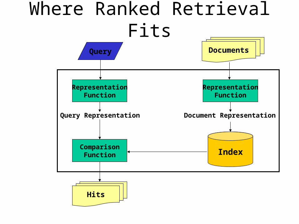
Where Ranked Retrieval Fits

DocumentsQuery

Hits

RepresentationFunction

RepresentationFunction

Query Representation Document Representation

ComparisonFunction Index

Ranked Retrieval Paradigm

• Perform a fairly general search– One designed to retrieve more than is needed

• Rank the documents in “best-first” order– Where best means “most likely to be relevant”

• Display as a list of easily skimmed “surrogates” – E.g., snippets of text that contain query terms

Advantages of Ranked Retrieval

• Leverages human strengths, covers weaknesses– Formulating precise queries can be difficult– People are good at recognizing what they want

• Moves decisions from query to selection time– Decide how far down the list to go as you read it

• Best-first ranking is an understandable idea

Ranked Retrieval Challenges

• “Best first” is easy to say but hard to do!– Computationally, we can only approximate it

• Some details will be opaque to the user– Query reformulation requires more guesswork

• More expensive than Boolean – Storing evidence for “best” requires more space– Query processing time increases with query length

Simple Example:Partial-Match Ranking

• Form all possible result sets in this order:– AND all the terms to get the first set– AND all but the 1st term, all but the 2nd, …– AND all but the first two terms, …– And so on until every combination has been done

• Remove duplicates from subsequent sets

• Display the sets in the order they were made– Document rank within a set is arbitrary

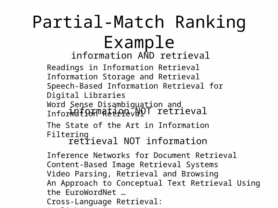
Partial-Match Ranking Exampleinformation AND retrieval

Readings in Information RetrievalInformation Storage and RetrievalSpeech-Based Information Retrieval for Digital LibrariesWord Sense Disambiguation and Information Retrieval

information NOT retrieval

The State of the Art in Information Filtering

Inference Networks for Document RetrievalContent-Based Image Retrieval SystemsVideo Parsing, Retrieval and BrowsingAn Approach to Conceptual Text Retrieval Using the EuroWordNet …Cross-Language Retrieval: English/Russian/French

retrieval NOT information

Agenda


Similarity-based ranking

• Probability-based ranking

What’s a Model?

• A construct to help understand a complex system– A particular way of “looking at things”

• Models inevitably make simplifying assumptions

Similarity-Based Queries

• Model relevance as “similarity”– Rank documents by their similarity to the query

• Treat the query as if it were a document– Create a query bag-of-words

• Find its similarity to each document

• Rank order the documents by similarity

• Surprisingly, this works pretty well!

Similarity-Based Queries

• Treat the query as if it were a document– Create a query bag-of-words

• Find the similarity of each document– Using the coordination measure, for example

• Rank order the documents by similarity– Most similar to the query first

• Surprisingly, this works pretty well!– Especially for very short queries

Document Similarity

• How similar are two documents?– In particular, how similar is their bag of words?

1

1

1

1: Nuclear fallout contaminated Montana.

2: Information retrieval is interesting.

3: Information retrieval is complicated.

1

1

1

1

1

1

nuclear

fallout

siberia

contaminated

interesting

complicated

information

retrieval

1

1 2 3

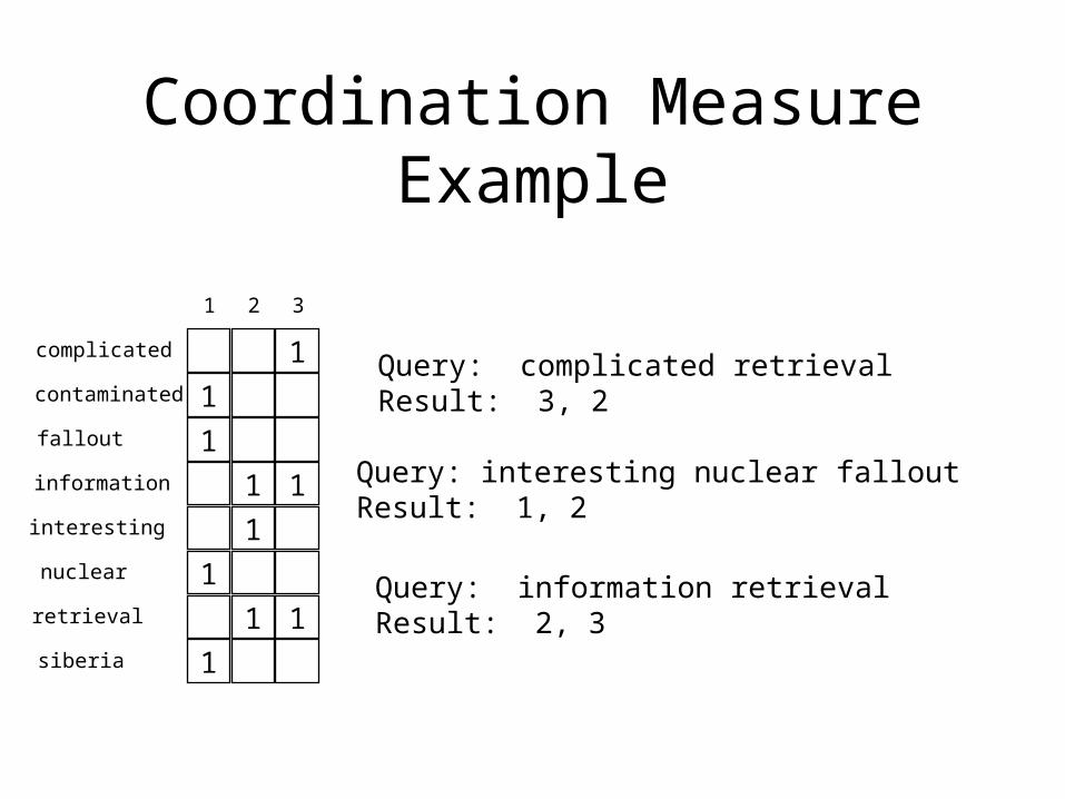
The Coordination Measure

• Count the number of terms in common– Based on Boolean bag-of-words

• Documents 2 and 3 share two common terms– But documents 1 and 2 share no terms at all

• Useful for “more like this” queries– “more like doc 2” would rank doc 3 ahead of doc 1

• Where have you seen this before?

Coordination Measure Example

1

1

1

1

1

1

1

1

1

nuclear

fallout

siberia

contaminated

interesting

complicated

information

retrieval

1

1 2 3

Query: complicated retrievalResult: 3, 2

Query: information retrievalResult: 2, 3

Query: interesting nuclear falloutResult: 1, 2

Vector Space Model

Postulate: Documents that are “close together” in vector space “talk about” the same things

t1

d2

d1

d3

d4

d5

t3

t2

θ

φ

Therefore, retrieve documents based on how close the document is to the query (i.e., similarity ~ “closeness”)

Counting Terms

• Terms tell us about documents– If “rabbit” appears a lot, it may be about rabbits

• Documents tell us about terms– “the” is in every document -- not discriminating

• Documents are most likely described well by rare terms that occur in them frequently– Higher “term frequency” is stronger evidence– Low “document frequency” makes it stronger still

McDonald's slims down spudsFast-food chain to reduce certain types of fat in its french fries with new cooking oil.NEW YORK (CNN/Money) - McDonald's Corp. is cutting the amount of "bad" fat in its french fries nearly in half, the fast-food chain said Tuesday as it moves to make all its fried menu items healthier.But does that mean the popular shoestring fries won't taste the same? The company says no. "It's a win-win for our customers because they are getting the same great french-fry taste along with an even healthier nutrition profile," said Mike Roberts, president of McDonald's USA.But others are not so sure. McDonald's will not specifically discuss the kind of oil it plans to use, but at least one nutrition expert says playing with the formula could mean a different taste.Shares of Oak Brook, Ill.-based McDonald's (MCD: down $0.54 to $23.22, Research, Estimates) were lower Tuesday afternoon. It was unclear Tuesday whether competitors Burger King and Wendy's International (WEN: down $0.80 to $34.91, Research, Estimates) would follow suit. Neither company could immediately be reached for comment.…

16 × said

14 × McDonalds

12 × fat

11 × fries

8 × new

6 × company, french, nutrition

5 × food, oil, percent, reduce,

taste, Tuesday

…

“Bag of Words”

A Partial Solution: TF*IDF• High TF is evidence of meaning• Low DF is evidence of term importance

– Equivalently high “IDF”

• Multiply them to get a “term weight” • Add up the weights for each query term

DF

NTFw

jiTF

iNDF

N

jiji

ji

logThen

document in appears term timesofnumber thebe Let

rmcontain te documents theof Let

documents ofnumber total thebe Let

,,

,

TF*IDF Example

4

5

6

3

1

3

1

6

5

3

4

3

7

1

nuclear

fallout

siberia

contaminated

interesting

complicated

information

retrieval

2

1 2 3

2

3

2

4

4

0.50

0.63

0.90

0.13

0.60

0.75

1.51

0.38

0.50

2.11

0.13

1.20

1 2 3

0.60

0.38

0.50

4

0.301

0.125

0.125

0.125

0.602

0.301

0.000

0.602

idfi

query: contaminated retrievalResult: 2, 3, 1, 4

tf ,i jwi j,

The Document Length Effect

• People want documents with useful parts– But scores are computed for the whole document

• Document lengths vary in many collections– So frequency could yield inconsistent resutls

• Two strategies– Adjust term frequencies for document length– Divide the documents into equal “passages”

Document Length Normalization

• Long documents have an unfair advantage– They use a lot of terms

• So they get more matches than short documents

– And they use the same words repeatedly• So they have much higher term frequencies

• Normalization seeks to remove these effects– Related somehow to maximum term frequency

“Cosine” Normalization• Compute the length of each document vector

– Multiply each weight by itself– Add all the resulting values– Take the square root of that sum

• Divide each weight by that length

Let be the unnormalized weight of term in document

Let be the normalized weight of term in document

Then

w i j

w i j

ww

w

i j

i j

i j

i j

i jj

,

,

,

,

,

2

Cosine Normalization Example

0.29

0.37

0.53

0.13

0.62

0.77

0.57

0.14

0.19

0.79

0.05

0.71

1 2 3

0.69

0.44

0.57

4

4

5

6

3

1

3

1

6

5

3

4

3

7

1

nuclear

fallout

siberia

contaminated

interesting

complicated

information

retrieval

2

1 2 3

2

3

2

4

4

0.50

0.63

0.90

0.13

0.60

0.75

1.51

0.38

0.50

2.11

0.13

1.20

1 2 3

0.60

0.38

0.50

4

0.301

0.125

0.125

0.125

0.602

0.301

0.000

0.602

idfi

1.70 0.97 2.67 0.87Length

tf ,i jwi j, wi j,

query: contaminated retrieval, Result: 2, 4, 1, 3 (compare to 2, 3, 1, 4)

Formally …

n

i ki

n

i ji

n

i kiji

kj

kjkj

ww

ww

dd

ddddsim

1

2,1

2,

1 ,,),(

Document Vector

Query Vector

Inner Product

Length Normalization

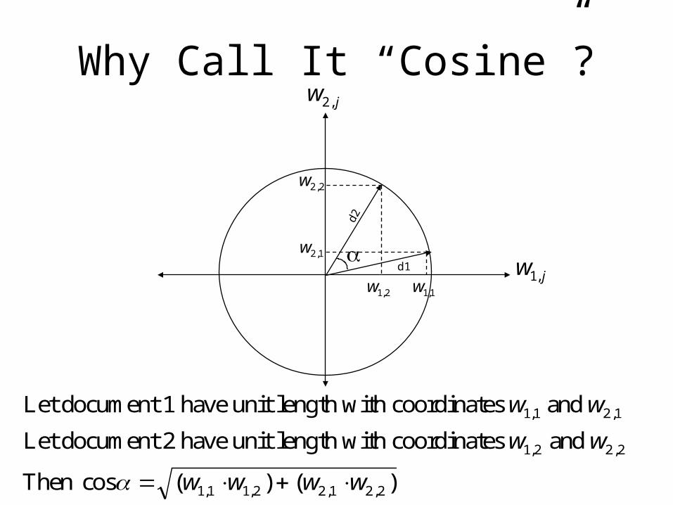
Why Call It “Cosine”?

d2

d1 w j1,

w j2,

w2 2,

w2 1,

w1 1,w1 2,

Let document 1 have unit length with coordinates and

Let document 2 have unit length with coordinates and

Then

w w

w w

w w w w

1 1 2 1

1 2 2 2

1 1 1 2 2 1 2 2

, ,

, ,

, , , ,cos ( ) ( )

Interpreting the Cosine Measure

• Think of query and the document as vectors– Query normalization does not change the ranking– Square root does not change the ranking

• Similarity is the angle between two vectors– Small angle = very similar– Large angle = little similarity

• Passes some key sanity checks– Depends on pattern of word use but not on length– Every document is most similar to itself

“Okapi BM-25” Term Weights

5.0

5.0log*

5.05.1

document ain termsofnumber average thebe Let

document in termsofnumber thebe Let

,

,,

j

j

jii

jiji

i

DF

DFN

TFL

L

TFw

L

iL

0.0

0.2

0.4

0.6

0.8

1.0

0 5 10 15 20 25

Raw TF

Oka

pi

TF 0.5

1.0

2.0

4.4

4.6

4.8

5.0

5.2

5.4

5.6

5.8

6.0

0 5 10 15 20 25

Raw DF

IDF Classic

Okapi

LL /

TF component IDF component

Passage Retrieval

• Another approach to long-document problem– E.g., break it up into coherent units

• Recognizing topic boundaries can be hard– Overlapping 300 word passages work well

• Use best passage rank as the document’s rank– Passage ranking can also help focus examination

Summary

• Goal: find documents most similar to the query

• Compute normalized document term weights– Some combination of TF, DF, and Length

• Sum the weights for each query term– In linear algebra, this is an “inner product” operation

Agenda


• Similarity-based ranking

Probability-based ranking

The Key Idea

• We ask “is this document relevant?”– Vector space: we answer “somewhat”– Probabilistic: we answer “probably”

• The key is to know what “probably” means– First, we’ll formalize that notion– Then we’ll apply it to ranking

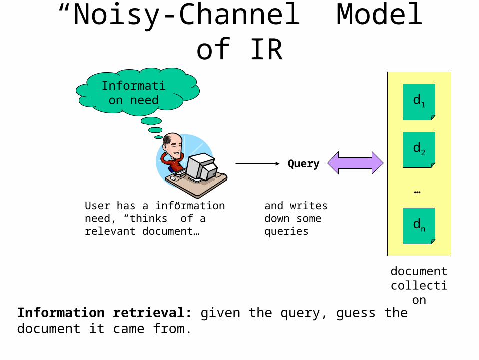
“Noisy-Channel” Model of IR

Information need

Query

User has a information need, “thinks” of a relevant document…

and writes down some queries

Information retrieval: given the query, guess the document it came from.

d1

d2

dn

document collection

…

Where do the probabilities fit?

Comparison Function

Representation Function

Query Formulation

Human Judgment

Representation Function

Retrieval Status Value

Utility

Query

Information Need Document

Query Representation Document Representation

Que

ry P

roce

ssin

g

Doc

umen

t P

roce

ssin

g

P(d is Rel | q)

Probabilistic Inference

• Suppose there’s a horrible, but very rare disease

• But there’s a very accurate test for it

• Unfortunately, you tested positive…

The probability that you contracted it is 0.01%

The test is 99% accurate

Should you panic?

Bayes’ Theorem

• You want to find

• But you only know– How rare the disease is– How accurate the test is

• Use Bayes’ Theorem (hence Bayesian Inference)

P(“have disease” | “test positive”)

)(

)()|()|(

BP

APABPBAP

Prior probability

Posterior probability

Applying Bayes’ Theorem

Two cases:1. You have the disease, and you tested positive2. You don’t have the disease, but you tested positive (error)

Case 1: (0.0001)(0.99) = 0.000099Case 2: (0.9999)(0.01) = 0.009999Case 1+2 = 0.010098

P(“have disease” | “test positive”)= (0.99)(0.0001) / 0.010098= 0.009804 < 1%

Don’t worry!

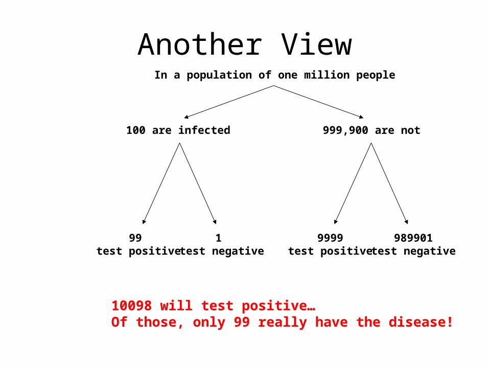
Another ViewIn a population of one million people

100 are infected 999,900 are not

99 test positive

1 test negative

9999test positive

989901test negative

10098 will test positive… Of those, only 99 really have the disease!

Probability

• Alternative definitions– Statistical: relative frequency as n – Subjective: degree of belief

• Thinking statistically– Imagine a finite amount of “stuff”– Associate the number 1 with the total amount– Distribute that “mass” over the possible events

Statistical Independence

• A and B are independent if and only if: P(A and B) = P(A) P(B)

• Independence formalizes “unrelated”– P(“being brown eyed”) = 85/100– P(“being a doctor”) = 1/1000– P(“being a brown eyed doctor”) = 85/100,000

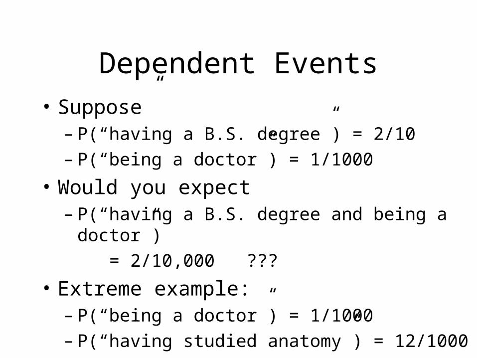
Dependent Events

• Suppose”– P(“having a B.S. degree”) = 2/10– P(“being a doctor”) = 1/1000

• Would you expect– P(“having a B.S. degree and being a doctor”)

= 2/10,000 ???

• Extreme example:– P(“being a doctor”) = 1/1000– P(“having studied anatomy”) = 12/1000

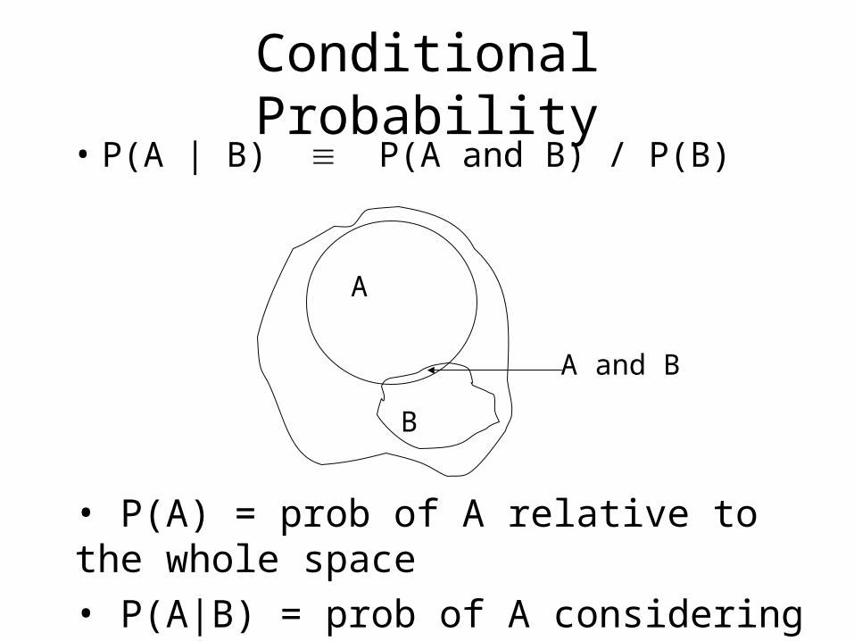
Conditional Probability• P(A | B) P(A and B) / P(B)

A

B

A and B

• P(A) = prob of A relative to the whole space

• P(A|B) = prob of A considering only the cases where B is known to be true

More on Conditional Probability

• Suppose– P(“having studied anatomy”) = 12/1000– P(“being a doctor and having studied anatomy”) = 1/1000

• Consider– P(“being a doctor” | “having studied anatomy”) = 1/12

• But if you assume all doctors have studied anatomy– P(“having studied anatomy” | “being a doctor”) = 1

Useful restatement of definition: P(A and B) = P(A|B) x P(B)

Some Notation

• Consider – A set of hypotheses: H1, H2, H3– Some observable evidence O

• P(O|H1) = probability of O being observed if we knew H1 were true



An Example

• Let– O = “Joe earns more than $100,000/year”

– H1 = “Joe is a doctor”

– H2 = “Joe is a college professor”

– H3 = “Joe works in food services”

• Suppose we do a survey and we find out– P(O|H1) = 0.6

– P(O|H2) = 0.07

– P(O|H3) = 0.001

• What should be our guess about Joe’s profession?

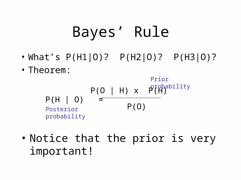
Bayes’ Rule

• What’s P(H1|O)? P(H2|O)? P(H3|O)?

• Theorem:

P(H | O) = P(O | H) x P(H)

P(O) Posteriorprobability

Priorprobability

• Notice that the prior is very important!

Back to the Example

• Suppose we also have good data about priors:– P(O|H1) = 0.6 P(H1) = 0.0001 doctor– P(O|H2) = 0.07 P(H2) = 0.001 prof– P(O|H3) = 0.001 P(H3) = 0.2 food

• We can calculate– P(H1|O) = 0.00006 / P(“earning >

$100K/year”)– P(H2|O) = 0.0007 / P(“earning > $100K/year”)– P(H3|O) = 0.0002 / P(“earning > $100K/year”)

Key Ideas

• Defining probability using frequency

• Statistical independence

• Conditional probability

• Bayes’ rule

Probability Ranking Principle• Assume binary relevance, document independence

– Each document is either relevant or it is not– Relevance of one doc reveals nothing about another

• Assume the searcher works down a ranked list– Seeking some number of relevant documents

• Theorem (provable from assumptions):– Documents should be ranked in order of decreasing

probability of relevance to the query,

P(d relevant-to q)

Language Models

• Probability distribution over strings of text– How likely is a string in a given “language”?

• Probabilities depend on what language we’re modeling

p1 = P(“a quick brown dog”)

p2 = P(“dog quick a brown”)

p3 = P(“быстрая brown dog”)

p4 = P(“быстрая собака”)

In a language model for English: p1 > p2 > p3 > p4

In a language model for Russian: p1 < p2 < p3 < p4

Unigram Language Model

• Assume each word is generated independently– Obviously, this is not true…– But it seems to work well in practice!

• The probability of a string, given a model:

k

iik MqPMqqP

11 )|()|(

The probability of a sequence of words decomposes into a product of the probabilities of individual words

A Physical Metaphor

• Colored balls are randomly drawn from an urn (with replacement)

P ( )P ( ) == (4/9) (2/9) (4/9) (3/9)

wordsM

P ( ) P ( ) P ( )

An Example

the man likes the woman0.2 0.01 0.02 0.2 0.01

multiply

P(s | M) = 0.00000008

P(“the man likes the woman”|M)= P(the|M) P(man|M) P(likes|M) P(the|M) P(man|M)= 0.00000008

P(w) w

0.2 the

0.1 a

0.01 man

0.01 woman

0.03 said

0.02 likes

…

Model M

Comparing Language Models

P(w) w

0.2 the

0.0001 yon

0.01 class

0.0005 maiden

0.0003 sayst

0.0001 pleaseth

…

Model M1

P(w) w

0.2 the

0.1 yon

0.001 class

0.01 maiden

0.03 sayst

0.02 pleaseth

…

Model M2

maidenclass pleaseth yonthe

0.00050.01 0.0001 0.00010.2

0.010.001 0.02 0.10.2

P(s|M2) > P(s|M1)

What exactly does this mean?

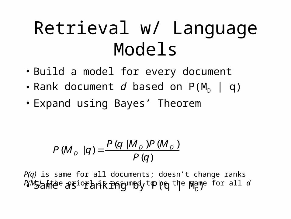
Retrieval w/ Language Models

• Build a model for every document

• Rank document d based on P(MD | q)

• Expand using Bayes’ Theorem

• Same as ranking by P(q | MD)

)(

)()|()|(

qP

MPMqPqMP DD

D

P(q) is same for all documents; doesn’t change ranksP(MD) [the prior] is assumed to be the same for all d

Visually …

Ranking by P(MD | q)…

Hey, what’s the probability this query came from you?

model1

Hey, what’s the probability that you generated this

query?

model1

is the same as ranking by P(q | MD)


model2


query?

model2


modeln


query?

modeln

… …

Ranking Models?


query?

model1

Ranking by P(q | MD)


query?

model2


query?

modeln

…

… is a model of document1

… is a model of document2

… is a model of documentn

… is the same as ranking documents

Building Document Models• How do we build a language model for a

document?

What’s in the urn?

M

Physical metaphor:

What colored balls and how many of each?

A First Try

• Simply count the frequencies in the document = maximum likelihood estimate

M P ( ) = 1/2

P ( ) = 1/4

P ( ) = 1/4

P(w|MS) = #(w,S) / |S|

Sequence S

#(w,S) = number of times w occurs in S|S| = length of S

Zero-Frequency Problem

• Suppose some event is not in our observation S– Model will assign zero probability to that event

M

P ( ) = 1/2

P ( ) = 1/4

P ( ) = 1/4

Sequence S

P ( )P ( ) =

= (1/2) (1/4) 0 (1/4) = 0

P ( ) P ( ) P ( )

!!

Why is this a bad idea?• Modeling a document

– A word not appearing doesn’t mean it’ll never appear…– Safe to assume that unseen words are rare, though

• Think of the document model as a topic– Many documents that can be written about a single topic– We try to guess the model is based on just one document

• Practical effect: assigning zero probability to unseen words forces exact match

Smoothing

P(w)

w

Maximum Likelihood Estimate

wordsallofcountwofcount

ML wp )(

The solution: “smooth” the word probabilities

Smoothed probability distribution

Implementing Smoothing

• Assign some small probability to unseen events– But remember to take away “probability mass”

from other events

• Some techniques are easily understood– Add one to all the frequencies (including zero)

• More sophisticated methods improve ranking

Recap: LM for IR

• Indexing-time: – Build a language model for every document

• Query-time Ranking– Estimate the probability of generating the query

according to each model– Rank the documents according to these

probabilities

Language Model Advantages

• Conceptually simple

• Explanatory value

• Exposes assumptions

• Minimizes reliance on heuristics

Key Ideas

• Probabilistic methods formalize assumptions– Binary relevance

– Document independence

– Term independence

– Uniform priors

– Top-down scan

• Natural framework for combining evidence– e.g., non-uniform priors

A Critique

• Most of the assumptions are not satisfied!– Searchers want utility, not relevance– Relevance is not binary– Terms are clearly not independent– Documents are often not independent

• Smoothing techniques are somewhat ad hoc

But It Works!

• Ranked retrieval paradigm is powerful– Well suited to human search strategies

• Probability theory has explanatory power– At least we know where the weak spots are– Probabilities are good for combining evidence

• Good implementations exist (e.g., Lemur)– Effective, efficient, and large-scale

Comparison With Vector Space

• Similar in some ways– Term weights based on frequency– Terms often used as if they were independent

• Different in others– Based on probability rather than similarity– Intuitions are probabilistic rather than geometric

A Complete System

• Perform an initial Boolean query– Balancing breadth with understandability

• Rerank the results– Using either Okapi or a language model– Possibly also accounting for proximity, links, …

One Minute Paper

• Which assumption underlying the probabilistic retrieval model causes you the most concern, and why?