Rao-Blackwellized Particle Filters forRecognizing Activities and Spatial Contextfrom Wearable Sensors

Alvin Raj1, Amarnag Subramanya2, Dieter Fox1, and Jeff Bilmes2

1University of Washington, Dept. of Computer Science & Engineering, Seattle, WA2University of Washington, Dept. of Electrical Engineering, Seattle, WA

1 Introduction

Recent advances in wearable sensing and computing devices and in fast prob-abilistic inference techniques make possible the fine-grained estimation of aperson’s activities over extended periods of time [6]. Such technologies enableapplications ranging from context aware computing to support for cognitivelyimpaired people to monitoring of activities of daily living.

The focus of our work is on providing accurate information about a per-son’s activities and environmental context in everyday environments based onwearable sensors and GPS devices. More specifically, we wish to estimate aperson’s motion type (such as walking, running, going upstairs/downstairs,or driving a vehicle) and whether a person is outdoors, inside a building, orin a vehicle. These activity estimates are combined with GPS informationso as to estimate the trajectory of the person along with information aboutwhich buildings the person enters. To do this, our approach assumes that thebounding boxes of buildings are known (extracted from satellite images).

Another emphasis of our work is on performing activity recognition basedon a minimum number of sensor devices. There are in fact a variety of systemsthat utilize multiple sensors and measurements taken all over the body [5,9]. Our approach, by contrast, attempts to produce as accurate as possibleactivity recognition requiring only one sensing device mounted only at onelocation on the body. Our reasoning for reducing the total number of sensorsis threefold: 1) it can be unwieldy for the person wearing the sensors to havemany such sensors and battery packs mounted all over the body, 2) we wishto minimize overall system cost, and 3) we wish to extend operational timebetween battery replacement/recharge.

In this paper, we show how Rao-Blackwellized particle filters can be ap-plied to efficiently estimate joint posteriors over a person’s activity and spatialcontext. Extensive experiments demonstrate that, by performing such jointinference, our system is able to generate more consistent estimates for a per-

2 Alvin Raj, Amarnag Subramanya, Dieter Fox, and Jeff Bilmes

Fig. 1. (left) Sensor board and (right) complete sensing package worn by a user.

son’s motion trajectory and activities. Our approach consistently outperformsa model that estimates a person’s activities and locations independently.

This paper is organized as follows. In Section 2, we give a brief overviewof our sensor system. Section 3 describes our activity model including allmodeling assumptions, inference, and learning algorithms. We discuss relatedwork in Section 4. Experiments are described in Section 5, followed by adiscussion and conclusions.

2 Wearable Sensor SystemOur customized wearable sensor system consists of a multi-sensor board, aHolux GPS unit with SIRF-III chipset, and an iPAQ PDA for data storage.The multi-sensor board shown in Fig. 1 is extremely compact, low-cost, anduses standard electronic components [6]. It weighs only 121g (about a quarterpound) including battery and processing hardware. Sensors include a 3-axisaccelerometer, microphones for recording speech and ambient sound, photo-transistors for measuring light conditions, and temperature and barometricpressure sensors. The overall cost per sensor board is approximately USD400. The time-stamped data collected on this device is transfered via a USBconnection to an iPAQ handheld computer. GPS data is transfered from thereceiver via Bluetooth to the PDA. The overall system is able to operate formore than 8 hours.

3 Activity Model3.1 OverviewThe complete dynamic Bayesian network for our activity model is shown inFig. 2, representing the probabilistic relationships between GPS measurements(gk, hk), sensor-board measurements mk, the person’s location lk, her motionvelocity vk, the type of motion sk she is performing, and the environment ek

she is in. We now describe the individual components starting at the sensorlevel of the model.

GPS measurements are separated into longitude / latitude information, gk,and horizontal dillusion of precision (hdop), hk. hdop provides information

Recognizing Activities and Spatial Context from Wearable Sensors 3

k−1

g kg k−1

hk−1 h k

Environment

Motion type

Velocity

Location

Sensor−board measurements

indoors, outdoors, vehicle

stationary, walking, runing, driving vehicle, going up/downstairs

(x,y) or building number

accelerometer, barometer, audio, light, ...

GPS (x,y)

GPS hdopGPS outlier (out) and offset (off)kok−1o

translation t and heading

k−1

θ

mkm

k−1e ke

vk

k−1s ks

lklk−1

v

Fig. 2. Dynamic Bayesian network for joint inference.

about the accuracy of the location information, which depends mostly onthe visibility and position of satellites. The node ok = (outk, offk) explicitlymodels GPS outliers and systematic GPS offset. Outliers typically occur whenthe person is inside a building or under trees. Unfortunately, outliers are notalways indicated by a high hdop value. GPS offset is due to systematic bias inthe estimates provided by the GPS unit. In our experience, this bias can beup to 10m, depending on the locations of satellites and atmospheric changes.

A GPS measurement gk depends on the person’s location, lk, the hdopvalue, hk, and the GPS outlier and offset values, ok. The likelihood is givenby

p(gk | lk, hk, ok) =N (gk; lk − offk, σ2

hk) if outk = 0

εN (gk; gk, σ2hk

) if outk = 1 (1)

That is, if the measurement is not an outlier, then the likelihood is given by aGaussian centered at the person’s location lk (shifted by an offset offk). Thevariance of the Gaussian is a linear function of the hdop value hk. In order tokeep a consistent likelihood ratio between outliers and non-outliers, we set theoutlier likelihood relative to the Gaussian likelihood of non-outlier measure-ments (using ε = 0.8 in our experiments). The probability of a measurementbeing an outlier depends on the previous outlier state, the hdop value, andthe environmental state (we set outk = 1 if the person is inside a buildingor has exited a building very recently). The offset value offk is modeled as aprocess with small Gaussian drift.

Sensor-board measurements mk consist of 3D acceleration, barometricpressure, temperature, visible and IR light intensity, and raw audio. We usethe boosted classifiers introduced by [6] to extract probability estimates for theperson’s instantaneous environment and motion state. These classifier outputsspecify the observation mk, which depends on the current environment andmotion state (see [10] for more details).Location lk = (xk, yk)T of the person is estimated in longitude / latitudecoordinates if the person is outside or driving a vehicle. If the person is inside

4 Alvin Raj, Amarnag Subramanya, Dieter Fox, and Jeff Bilmes

a building, we only estimate which building the person is in, not the actuallocation inside the building. The location at time k depends on the person’sprevious location lk−1 and motion vk−1, and on the current environment. Ifek = inside, then p(lk) is non-zero only if lk is inside the bounding box of abuilding. We extract the bounding boxes of buildings from satellite images.

Velocity represents the motion between locations at consecutive points intime. We adopt a piecewise linear motion model on polar velocity coordinatesvk = (tk, θk)T , namely translational speed, tk, and heading direction, θk. Weassume that the heading at time k only depends on the previous heading andtranslation speed, where the size in rotation (heading change) depends on thespeed. We model this relationship via a speed dependent Gaussian varianceσ2

tk−1with

p(θk|θk−1, tk−1) ∼ N (θk; θk−1, σ2tk−1

). (2)

The translational speed tk depends on the previous speed tk−1 and thecurrent motion state sk using the following product model:

p(tk | tk−1, sk) ∝ N (tk; tk−1, σ2a)

I∑i=1

αsk[i] N (tk;µsk[i], σ2sk[i]). (3)

The first factor is a Gaussian centered at the previous speed, where σ2a rep-

resents acceleration. The dependency on the motion state, sk, is implementedby the second factor, a mixture of I Gaussians, where αsk[i] represents theweight of the i-th mixture component, given state sk (similar to [7]). For in-stance, if the motion state is walking, then most weight is on the componentwith a mean at typical walking speed. In the driving mode, the mixturecomponents are more spread out, with significant weight on higher velocities.

Motion states represent different types of motion a person can be involvedin. In our current system, these states include S = {stationary, walking,running, going up/down stairs, driving vehicle}. The motion state sk

depends on the previous motion state sk−1 and the current environment ek.

Environment captures the person’s spatial context, which is E = {indoors,outdoors,vehicle}. The edge between ek and sk allows the system to modelboth soft and hard constraints between the motion state and the environ-ment. For example, whenever the environment is in the indoors or outdoorsstate, we a priori preclude driving from being a possible value of the mo-tion type (i.e., it has zero probability). Moreover, other “soft constraints” areimposed by the fact that the two nodes are related probabilistically, and theprobabilities are learned automatically (see Section 3.3).

3.2 Inference

During inference, our system estimates a joint posterior distribution over thecomplete state space. Unfortunately, exact inference is not tractable in ourmodel due to its combination of discrete and continuous hidden states. In [10]

Recognizing Activities and Spatial Context from Wearable Sensors 5

we show how to perform efficient inference using a discretization of the statespace along with an adaptive pruning strategy. Here, we describe how Rao-Blackwellized particle filters (RBPF) can be applied for efficient inferencein such a model. We omit a comprehensive derivation of our algorithm, itscorrectness can be shown similar to the derivations given in [3, 2, 7].

Just like regular particle filters, RBPFs represent posteriors over a statespace by temporal sets of weighted samples: Sk = {s(i)

k , w(i)k | 1 ≤ i ≤ N}. A

particle filter updates such sample sets according to a sampling procedure of-ten referred to as sequential importance sampling with re-sampling (SISR, seealso [11]). RBPFs derive their efficiency from a factorization of the state space,where posteriors over one part of the state space are represented by samples,and posteriors over the remaining parts are estimated exactly, conditioned oneach sample. We rely on the following factorization:

p(ek, sk, l1:k, v1:k, o1:k | m1:k, g1:k)= p(ek, sk | l1:k, v1:k, o1:k,m1:k, g1:k) p(l1:k, v1:k, o1:k | m1:k, g1:k). (4)

Our RBPF algorithm samples the variables in the second factor of (4), andcomputes exact posteriors over the variables in the first factor. Accordingly,each particle s

(i)k has the form

s(i)k =

⟨p(i)k (ek, sk), l(i)1:k, v

(i)1:k, o

(i)1:k

⟩,

where l(i)1:k, v

(i)1:k, o

(i)1:k are sampled values, and p

(i)k (ek, sk) is a distribution over

the current environment and motion state corresponding to these values.Table 1 summarizes our RBPF algorithm for iteratively updating sample

sets over time. The algorithm accepts as input a sample set Sk−1 along withthe most recent sensor board measurement mk, the most recent GPS mea-surement gk and the most recent hdop hk. Each iteration of the loop startingin Step 2 generates a new particle. In Step 3, the distribution over ek and sk

is predicted based on the particle’s previous distribution over these variables.This prediction is performed by marginalization over the previous time step:

p(i)k (ek, sk) =

∑ek−1,sk−1

p(sk | ek, sk−1) p(ek | ek−1) p(ek−1, sk−1) (5)

In Step 4, the algorithm generates a sample from this predictive distribution,which is used in Steps 6–8 to sample the particle’s motion and GPS outliervalues. Step 5 updates the location based on the previous location and motion,and the current environment. The function f distinguishes between locationsinside and outside buildings. If e

(i)k = indoors and l

(i)k−1 was in a building

bounding box, then f(l(i)k−1, v(i)k−1, e

(i)k ) = l

(i)k−1, otherwise l

(i)k is computed by

shifting l(i)k−1 according to the motion v

(i)k−1. f additionally models a motion

away from the building if the previous location was inside a bounding box.Once l

(i)k , v

(i)k , and o

(i)k are sampled, the particle’s distribution over envi-

ronment and motion state is updated in Step 9 using the following equation:

6 Alvin Raj, Amarnag Subramanya, Dieter Fox, and Jeff Bilmes

Inputs:

Previous sample set: Sk−1 = {s(i)k−1, w

(i)k−1 | 1 ≤ i ≤ N}

Observations: gk, mk, hk

1. Sk = ∅ // Initialize

2. for i = 1, . . . , N do // Generate samples

// Predictive distribution over environment and motion state

3. Compute bp(i)k (ek, sk) using (5) with prior p

(i)k−1(ek−1, sk−1)

4. Sample (e(i)k , s

(i)k ) ∼ bp(i)

k (ek, sk)

// Update location using previous location, motion, and env.

5. l(i)k = f(l

(i)k−1, v

(i)k−1, e

(i)k )

// Sample motion and GPS outlier conditioned on (e(i)k , s

(i)k )

6. Sample θ(i)k ∼ p(θ

(i)k | θ

(i)k−1, t

(i)k ) // Heading, see (2)

7. Sample t(i)k ∼ p(t

(i)k | t

(i)k−1, s

(i)k ) // Translation velocity, see (3)

8. Sample o(i)k ∼ p(o

(i)k | o

(i)k−1, hk, e

(i)k ) // Outlier

// Posterior distribution over environment and motion state

9. Compute p(e(i)k , s

(i)k ) using (6) based on l

(i)k , v

(i)k , o

(i)k and bp(e

(i)k , s

(i)k ).

// Update particle weight

10. Calculate w(i)k using normalization factor of Step 9 and GPS likelihood (1).

11. endfor

12. Multiply / discard samples in Sk based on normalized weights wk

13. return Sk

Table 1. RBPF for joint inference over environment, motion state, and location.

p(i)k (ek, sk) ∝ p

(i)k (ek, sk) p(l(i)k |ek) p(o(i)

k |ek, hk) p(v(i)k |sk) p(mk|ek, sk) (6)

Since the sampling steps 5–8 have not considered the most recent observations,each particle still needs to receive an importance weight, which is given bythe normalization factor computed in (6), times the likelihood of the GPSmeasurement defined in (1). Finally, in Step 12, the particles are re-sampled.

3.3 Parameter Learning

The parameters of our model are learned using labeled training data. To learnthe mapping of raw sensor board measurements to binary classifiers, we usea technique introduced by Lester and colleagues [6]. This approach extractsapproximately 650 features from short temporal windows of sensor data andthen uses boosting to learn sequences of decision stumps that are combinedto form binary classifiers [10]. The observation model for these classifiers isthen trained along with the parameters related to ek and sk using standardmaximum likelihood training based on the labeled data. The translationalvelocity model (3) is learned using EM to get a mixture of Gaussians for eachmotion state. The only parameters set manually are those related to GPSnoise and outlier detections.

Recognizing Activities and Spatial Context from Wearable Sensors 7

4 Related Work

Recently, estimating activities from wearable sensors has received significantattention especially in the ubiquitous computing and artificial intelligencecommunities. Bao and Intille [1] use multiple accelerometers placed on a per-son’s body to estimate activities such as standing, walking, or running. Kernand colleagues [5] and Lukowicz et al. [9] added a microphone to a similar setof accelerometers in order to extract additional context information. Thesetechniques rely on Gaussian observation models and dimensionality reductiontechniques such as PCA and LDA to generate observation models from thelow-level sensor data or features extracted thereof. These approaches feed thesensor data or features into static classifiers [1, 4], a bank of temporally in-dependent HMMs [6], or multi-state HMMs [5] in order to perform temporalsmoothing. None of these approaches estimates a user’s spatial context.

To learn low-level sensor-board classifiers we rely on the approach intro-duced by Lester et al. [6], who showed how to apply boosting in the context ofsensor-based activity recognition. In contrast to the discrete inference systemused in [10], the RBPF algorithm described in this paper produces more accu-rate location traces and provides more flexibility in handling GPS outliers. In[10], we also showed how virtual evidence can be used to learn activity modelsfrom sparsely labeled data.

Using location for activity recognition has been the focus of other work.For instance, Liao and colleagues [7] showed how to learn a person’s outdoortransportation routines from GPS data. More recently, the same authors pre-sented a technique for jointly determining a person’s activities and her signif-icant places [8]. However, these approaches are very limited in their accuracydue to the fact that they only rely on location information.

5 Experiments

Our system was evaluated by an outside team as part of the DARPA ASSISTprogram. Our goal in this program is to develop techniques that can auto-matically generate reports that summarize and visualize relevant informationcollected by a soldier during a mission. The current focus of our research ison providing an accurate trace of where the person went, which buildings sheentered, and how she moved between places.

The accuracy of our inference system was tested on a set of sequencescollected via the ASSIST program (see Fig. 3). The environmental stateswere indoors, outdoors, and vehicle, and the activities were stopped, walk,run, drive, and going up/downstairs. In each test run, a soldier and one ofour team members followed an exactly specified activity sequence by movingbetween marked waypoints. The resulting 28 traces provided about 2 hoursof fully labeled training and test data. In order to test the accuracy of thesystem, we divided the data into 4 sets, each containing 7 randomly selectedtraces (sampling without replacement). We then performed four runs, duringwhich, each of the 4 sets was used for testing, while the remaining 3 sets wereused for training. Our RBPF algorithm used 2,000 particles for inference,

8 Alvin Raj, Amarnag Subramanya, Dieter Fox, and Jeff Bilmes

Fig. 3. Experimental setup: (left) Part of the evaluation area with waypoints. Thesubjects followed fully scripted traversals through the area. (right) A soldier and oneof our team members wore a sensor system. Ground truth annotations were providedby four additional observers equipped with stop watches and audio recorders.

State stopped walk run up down drive

No GPS 71.6 80.2 80.8 58.9 60.2 80.0

RBPF 65.3 79.1 74.8 36.3 36.3 93.6

Env. outdoor indoor vehicle

No GPS 94.1 87.1 88.0

RBPF 94.4 85.9 93.6

Fig. 4. Accuracy (number of correct frames/total number of frames): (left) Percent-age accuracies in detecting motion state and environment. Results are given for anHMM that ignores GPS and for our RBPF. (right) Raw GPS trace (gray) and traceestimated by our RBPF (black). The RBPF trace is aligned such that it enters andexits the building at the correct time and location. Overall, the spatial consistencyof RBPF traces is 92.8% vs. 33.8% for raw GPS.

which was performed in real-time on an Intel 3.2 GHz desktop PC with about1 GB of RAM. To extract an activity and location sequence from our RBPF,we used the history of the most likely particle at the end of each test run.

The table in Fig. 4 compares the accuracy of our system to the accuracyof the Viterbi sequences extracted by a hidden Markov model that ignoresinformation provided by the GPS sensor. As can be seen, the performance ofthe RBPF is not better than that of the hidden Markov Model. This howeverdoes not indicate that, GPS information is not useful for improving activityrecognition performance (see [10]). The above trend may be due to the wayparameters are learnt in the two approaches. Whilst, in the case of a hiddenMarkov model, all parameters are jointly trained, the same is not true in thecase of the RBPF.

To assess the impact of our joint inference on the accuracy of locationtraces, we proceeded as follows. Whenever the person was inside a building,we determined how often the raw GPS trace and the trace estimated by ourRBPF was inside the bounding box of that building. Averaged over all testtraces, our RBPF algorithm improved this accuracy from 8.7% for raw GPSto 85.9%. One example trace is shown in the right panel in Fig. 4. As can beseen, our RBPF is able to correctly align the location trace using informationabout the buildings.

Recognizing Activities and Spatial Context from Wearable Sensors 9

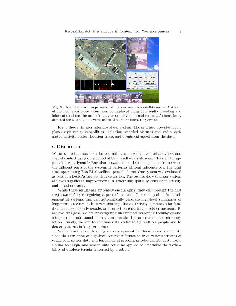
Fig. 5. User interface: The person’s path is overlayed on a satellite image. A streamof pictures taken every second can be displayed along with audio recording andinformation about the person’s activity and environmental context. Automaticallydetected faces and audio events are used to mark interesting events.

Fig. 5 shows the user interface of our system. The interface provides movieplayer style replay capabilities, including recorded pictures and audio, esti-mated activity states, location trace, and events extracted from the data.

6 Discussion

We presented an approach for estimating a person’s low-level activities andspatial context using data collected by a small wearable sensor device. Our ap-proach uses a dynamic Bayesian network to model the dependencies betweenthe different parts of the system. It performs efficient inference over the jointstate space using Rao-Blackwellized particle filters. Our system was evaluatedas part of a DARPA project demonstration. The results show that our systemachieves significant improvements in generating spatially consistent activityand location traces.

While these results are extremely encouraging, they only present the firststep toward fully recognizing a person’s context. Our next goal is the devel-opment of systems that can automatically generate high-level summaries oflong-term activities such as vacation trip diaries, activity summaries for fam-ily members of elderly people, or after action reporting of soldier missions. Toachieve this goal, we are investigating hierarchical reasoning techniques andintegration of additional information provided by cameras and speech recog-nition. Finally, we aim to combine data collected by multiple people and todetect patterns in long-term data.

We believe that our findings are very relevant for the robotics communitysince the extraction of high-level context information from various streams ofcontinuous sensor data is a fundamental problem in robotics. For instance, asimilar technique and sensor suite could be applied to determine the naviga-bility of outdoor terrain traversed by a robot.

10 Alvin Raj, Amarnag Subramanya, Dieter Fox, and Jeff Bilmes

Acknowledgments

The authors would like to thank Tanzeem Choudhury, Jonathan Lester, andGaetano Borriello for useful discussions and for making their feature learningcode available. Additional thanks go to the Intel Research Lab in Seattle forproviding the sensor boards used in this research, to Hanna Pasula for devel-oping the user interface and to the NIST evaluation team for their extraordi-nary effort in preparing and running the evaluation. This work has partly beensupported by DARPA’s ASSIST and CALO Programmes (contract numbers:NBCH-C-05-0137, SRI subcontract 27-000968), and by the NSF Human andSocial Dynamics (HSD) program under contract number IIS-0433637.

References

1. L. Bao and S Intille. Activity recognition from user-annotated accelerationdata. In Proc. of the International Conference on Pervasive Computing andCommunications, 2004.

2. H.H. Bui, S. Venkatesh, and G. West. Policy recognition in the abstract hiddenmarkov model. Journal of Artificial Intelligence Research (JAIR), 17, 2002.

3. A. Doucet, J.F.G. de Freitas, K. Murphy, and S. Russell. Rao-Blackwellisedparticle filtering for dynamic Bayesian networks. In Proc. of the Conference onUncertainty in Artificial Intelligence (UAI), 2000.

4. J. Ho and S. Intille. Using context-aware computing to reduce the perceivedburden of interruptions from mobile devices. In Proc. of the Conference onHuman Factors in Computing Systems (CHI), 2005.

5. N. Kern, B. Schiele, and A. Schmidt. Recognizing context for annotating a livelife recording. Personal and Ubiquituous Computingd, 2005.

6. J. Lester, T. Choudhury, N. Kern, G. Borriello, and B. Hannaford. A hybriddiscriminative-generative approach for modeling human activities. In Proc. ofthe International Joint Conference on Artificial Intelligence (IJCAI), 2005.

7. L. Liao, D. Fox, and H. Kautz. Learning and inferring transportation routines.In Proc. of the National Conference on Artificial Intelligence (AAAI), 2004.

8. L. Liao, D. Fox, and H. Kautz. Hierarchical conditional random fields for GPS-based activity recognition. In S. Thrun, H. Durrant-Whyte, and R. Brooks, edi-tors, Robotics Research: The Eleventh International Symposium, Springer Tractsin Advanced Robotics (STAR). Springer Verlag, 2006.

9. P. Lukowicz, J. Ward, H. Junker, M. Stager, G. Troster, A. Atrash, andT. Starner. Recognizing workshop activity using body worn microphones andaccelerometers. In Proc. of Pervasive Computing, 2004.

10. A. Subramanya, A. Raj, J. Bilmes, and D. Fox. Recognizing activities and spatialcontext from wearable sensors. In Proc. of the Conference on Uncertainty inArtificial Intelligence (UAI), 2006.

11. S. Thrun, W. Burgard, and D. Fox. Probabilistic Robotics. MIT Press, Cam-bridge, MA, September 2005. ISBN 0-262-20162-3.