Embed Size (px)
Citation preview

1
A MANUAL FOR RAPID BOTANIC SURVEY
(RBS) AND MEASUREMENT OF
VEGETATION BIOQUALITY W.D. Hawthorne & C. A. M. Marshall, June 2016
2
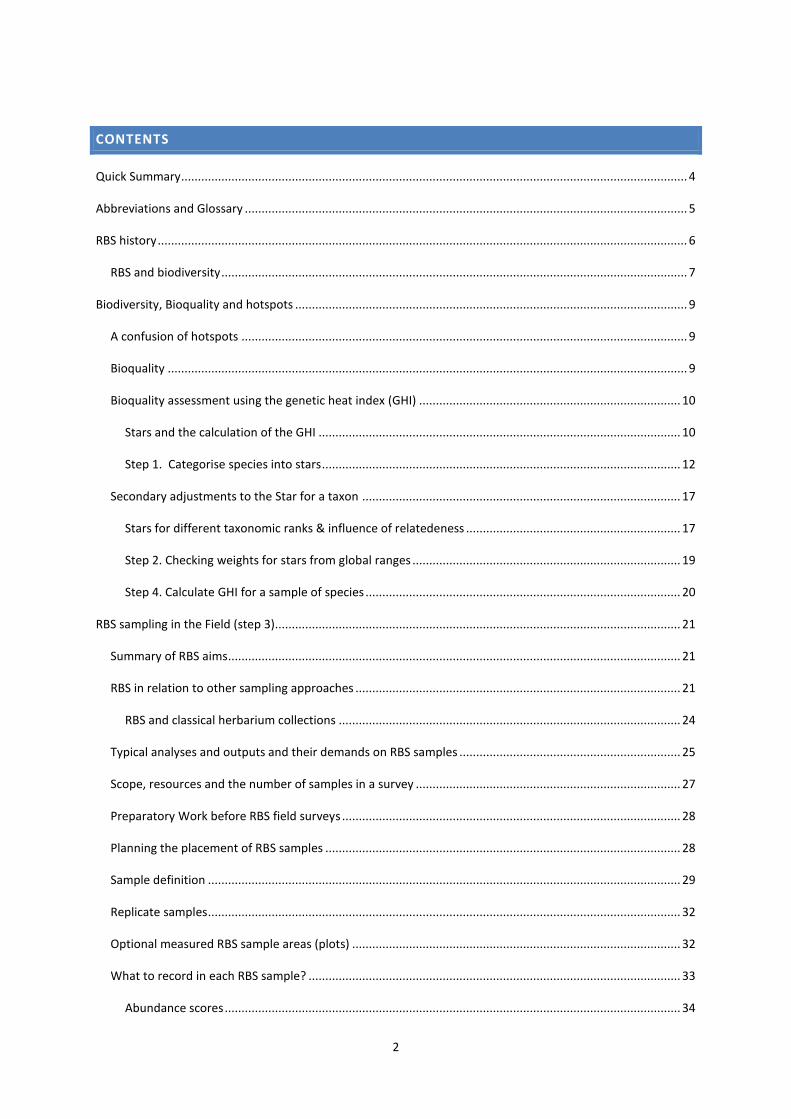
CONTENTS
Quick Summary ....................................................................................................................................................... 4
Abbreviations and Glossary .................................................................................................................................... 5
RBS history .............................................................................................................................................................. 6
RBS and biodiversity ........................................................................................................................................... 7
Biodiversity, Bioquality and hotspots ..................................................................................................................... 9
A confusion of hotspots ..................................................................................................................................... 9
Bioquality ........................................................................................................................................................... 9
Bioquality assessment using the genetic heat index (GHI) .............................................................................. 10
Stars and the calculation of the GHI ............................................................................................................ 10
Step 1. Categorise species into stars ........................................................................................................... 12
Secondary adjustments to the Star for a taxon ............................................................................................... 17
Stars for different taxonomic ranks & influence of relatedeness ................................................................ 17
Step 2. Checking weights for stars from global ranges ................................................................................ 19
Step 4. Calculate GHI for a sample of species .............................................................................................. 20
RBS sampling in the Field (step 3)......................................................................................................................... 21
Summary of RBS aims ....................................................................................................................................... 21
RBS in relation to other sampling approaches ................................................................................................. 21
RBS and classical herbarium collections ...................................................................................................... 24
Typical analyses and outputs and their demands on RBS samples .................................................................. 25
Scope, resources and the number of samples in a survey ............................................................................... 27
Preparatory Work before RBS field surveys ..................................................................................................... 28
Planning the placement of RBS samples .......................................................................................................... 28
Sample definition ............................................................................................................................................. 29
Replicate samples ............................................................................................................................................. 32
Optional measured RBS sample areas (plots) .................................................................................................. 32
What to record in each RBS sample? ............................................................................................................... 33
Abundance scores ........................................................................................................................................ 34

3
Canopy tree counts ...................................................................................................................................... 34
Relating general abundance and tree count data........................................................................................ 36
Recording local perceptions of vegetation with RBS ............................................................................................ 37
How does it work? ............................................................................................................................................ 37
Processing Specimens and Data ........................................................................................................................... 39
Examples of RBS projects and Bioquality Maps .................................................................................................... 40
Ghana’s forest zone ......................................................................................................................................... 41
Liberia, Nimba county ...................................................................................................................................... 42
Trinidad and Tobago ........................................................................................................................................ 43
Clients and partners.............................................................................................................................................. 44
For more information ........................................................................................................................................... 44
References ............................................................................................................................................................ 45
Appendix A: Notes on RBS Logistics ..................................................................................................................... 48
Organisation of field team ............................................................................................................................... 48
Identification and Herbarium work associated with RBS ................................................................................. 49
What resources do you need for a typical RBS? .............................................................................................. 49
Data arrangement and input ............................................................................................................................ 51
Sample names (sampname) ......................................................................................................................... 51
Major data types .......................................................................................................................................... 52
Sample RBS field form .......................................................................................................................................... 54
Star framework definitions implemented in Chile, Maule región 2009 ............................................................... 55
To cite this publication:
Hawthorne, W.D. & C. A. M. Marshall. A Manual for Rapid Botanic Survey (RBS) and measurement of vegetation
bioquality. Published online, June 2016. Department of Plant Sciences, University of Oxford, U.K.

4
QUICK SUMMARY
Rapid Botanic Survey (RBS) is primarily a field survey methodology for assessing species-rich plant communities,
but it is associated with a range of non-field activities, analyses and outputs that can be considered part of RBS
in a broad sense. This document is about the full range of typical RBS activities, from field to herbarium to
database to output.
RBS outputs are used for mapping vegetation and prioritising areas for different management purposes,
including conservation. RBS activities integrate species and community level assessments. RBS is particularly
appropriate in species-rich, incompletely explored vegetation, but could be used in any plant community. RBS
data are used to determine the main patterns of floristic variation in plant communities across a landscape. RBS
is also used, even in well-known vegetation, for measuring bioquality ‘temperature’: the degree to which a
sample is a biodiversity hotspot. RBS can be applied at any scale; it has been used to plan national and regional
conservation strategies, as well as local Environmental Impact Assessments (EIAs).
RBS builds on a foundation of herbarium data and provides a generally more complete and less biased picture
of plant biogeographic and ecological patterns than is available from herbaria alone. A typical survey involves
databasing some existing herbarium and published data of various types, and enumeration of a suite of new
RBS-specific samples in the field. The new samples fill the often substantial gaps in knowledge about plant
distribution and provide data on a cross-section of habitats in a defined survey area, using a standardised
approach.
The field survey tells us where each plant species lives within sampled landscapes. The background research
meanwhile leads to the categorisation, into ‘Stars’, of the global rarity of each species as a basis for highlighting
the global significance of local populations and vegetation patches. Plant communities, even local associations
of species occupying a few square metres, are scored or evaluated based on the species found there and other
local information collected during the surveys. The way in which Star ratings feed into community level
“bioquality” valuations is described on p. 9.
Whilst biodiversity hotspots have been crudely and ambiguously defined on the broad global scale, RBS aims to
achieve greater precision, higher resolution, practicality and transparency in biodiversity hotspot research.
Global plant biodiversity is being eroded daily, and ideal solutions to its conservation are not going to be possible
soon enough in many areas. One of the premises of RBS is that it is essential to make the most of what can be
assessed with limited resources, rather than waiting for perfect answers. RBS promotes successive
approximation and encourages fuzzy logic, when crisp logic and detailed studies would not lead anywhere fast
enough. The RBS framework provides objective, transparent and repeatable, best-available answers that are
open to refinement if time allows. This is one of the key differences between RBS and various other, ‘Ivory Tower’
approaches to biodiversity evaluation. Whilst the bull-dozers push back nature throughout the world, RBS places
pragmatism before academic purity in a bid to do something before the subject matter disappears.
It is possible to define and use Star ratings and measure bioquality without RBS samples; and to make good use
of RBS sample data without defining Stars. If you are interested in using RBS for purposes other than bioquality
evaluation, skip to page 7.
RBS-derived data form a good foundation for studies in many related disciplines, for example the impacts of
development or climate change on biodiversity, or studies of possible or actual impacts on species distribution.
5
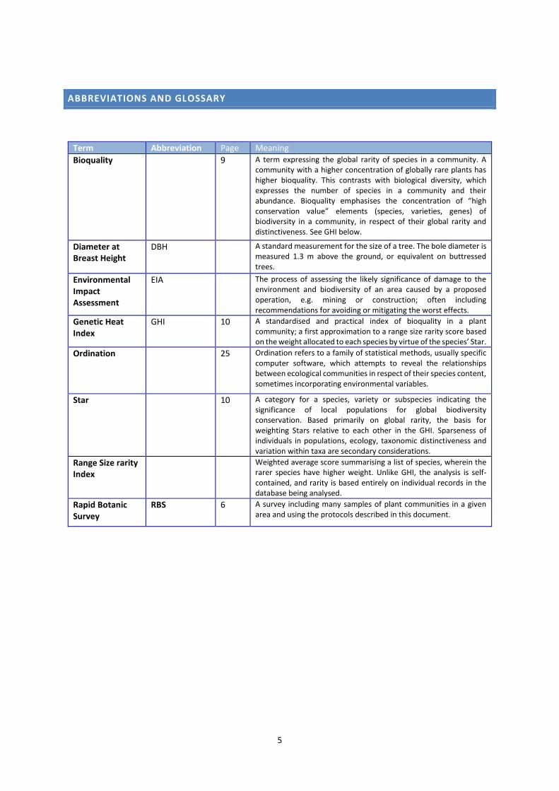
ABBREVIATIONS AND GLOSSARY
Term Abbreviation Page Meaning
Bioquality 9 A term expressing the global rarity of species in a community. A community with a higher concentration of globally rare plants has higher bioquality. This contrasts with biological diversity, which expresses the number of species in a community and their abundance. Bioquality emphasises the concentration of “high conservation value” elements (species, varieties, genes) of biodiversity in a community, in respect of their global rarity and distinctiveness. See GHI below.
Diameter at Breast Height
DBH A standard measurement for the size of a tree. The bole diameter is measured 1.3 m above the ground, or equivalent on buttressed trees.
Environmental Impact Assessment
EIA The process of assessing the likely significance of damage to the environment and biodiversity of an area caused by a proposed operation, e.g. mining or construction; often including recommendations for avoiding or mitigating the worst effects.
Genetic Heat Index
GHI 10 A standardised and practical index of bioquality in a plant community; a first approximation to a range size rarity score based on the weight allocated to each species by virtue of the species’ Star.
Ordination 25 Ordination refers to a family of statistical methods, usually specific computer software, which attempts to reveal the relationships between ecological communities in respect of their species content, sometimes incorporating environmental variables.
Star 10 A category for a species, variety or subspecies indicating the significance of local populations for global biodiversity conservation. Based primarily on global rarity, the basis for weighting Stars relative to each other in the GHI. Sparseness of individuals in populations, ecology, taxonomic distinctiveness and variation within taxa are secondary considerations.
Range Size rarity Index
Weighted average score summarising a list of species, wherein the rarer species have higher weight. Unlike GHI, the analysis is self-contained, and rarity is based entirely on individual records in the database being analysed.
Rapid Botanic Survey
RBS 6 A survey including many samples of plant communities in a given area and using the protocols described in this document.
6
RBS HISTORY
RBS and associated methods for analysing and using RBS data were originally designed for rapid assessment of
rain forest biodiversity in Africa, but RBS has since been used in other continents and vegetation types.
The sampling method was originally inspired by:
Plant community lists on herbarium labels, for instance: “this species is abundant in rocky, limestone
ravines on the east of the hill, with Impatiens blogsii, Cynometra webberi, Julbernardia, Asteranthe
asterias, Croton jacquesii”. This type of herbarium-based, label information is like a cut-down version
of an RBS sample, though the species lists are usually incomplete or at least of unknown completeness
and bias, and provide no means for checking the accuracy of the species listed.
Some of the aspects of field survey associated with Braun-Blanquet phytosociology, notably respect
for the value of subjective, surveyor’s choice of representative sample sites (Westhoff & van der Maarel
1978; Wikum & Shanholtzer, 1978). This method was designed for European types of vegetation, is not
ideal for rainforest, and the samples (relevés) are measured, unlike typical RBS samples.
A national forest type survey in Ghana by Swaine and Hall (Hall & Swaine, 1981), which included a
subset of unmeasured, so-called ‘B’ samples, to help interpolate data from a network of larger
measured plots. Swaine and Hall (1976) had established in Ghana that records of just 30 random
species provided enough information to identify the forest types established using full 50-150 species
lists from measured 25 x 25m plots. RBS samples are similar to these B plots in that they are
unmeasured, but are in general are more thorough samples of the local landscape unit.
RBS-like sampling evolved from these approaches during a survey of coastal forests in Tanzania and Kenya,
where the sample units were called ‘sublocalities’ (Hawthorne et al., 1981; Hawthorne, 1984, 1993a). The
protocol was subsequently developed into its current form in a national plant biodiversity survey of Ghana
(Hawthorne & Abu Juam, 1995; Hawthorne, 1996), complementing a national forest tree inventory. The
approach was initially designed to make maximum use of available data sources, including herbaria, plot based
samples and published, whole-forest check-lists. RBS outputs have subsequently had a prominent influence in
decisions about protected areas and objective allocation of global biodiversity funds in Ghana (Hawthorne et al.,
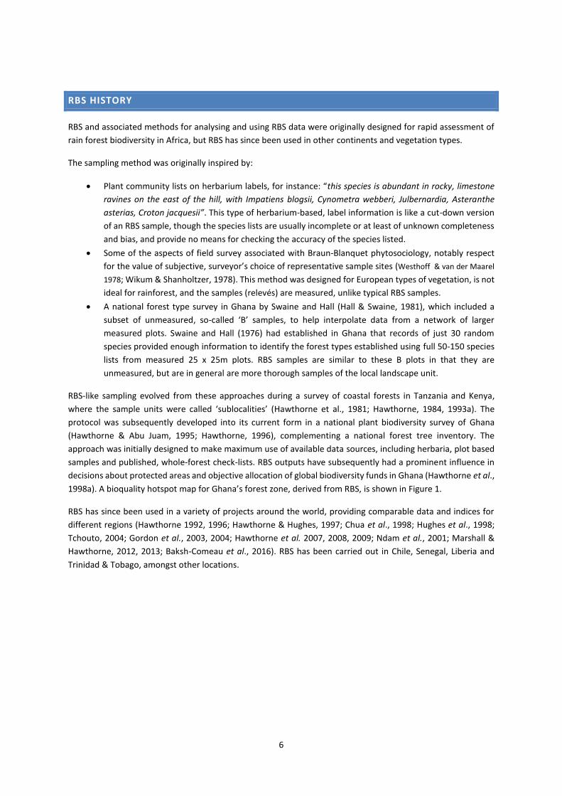
1998a). A bioquality hotspot map for Ghana’s forest zone, derived from RBS, is shown in Figure 1.
RBS has since been used in a variety of projects around the world, providing comparable data and indices for
different regions (Hawthorne 1992, 1996; Hawthorne & Hughes, 1997; Chua et al., 1998; Hughes et al., 1998;
Tchouto, 2004; Gordon et al., 2003, 2004; Hawthorne et al. 2007, 2008, 2009; Ndam et al., 2001; Marshall &
Hawthorne, 2012, 2013; Baksh-Comeau et al., 2016). RBS has been carried out in Chile, Senegal, Liberia and
Trinidad & Tobago, amongst other locations.
7
.
Figure 1 Ghana, showing forest reserves as outlines. The colours and the apparent landscape altitude indicate
bioquality. Note the red ‘peaks’ or hotspots of GHI in the SW (species rich, wet evergreen forest); and around
the south and west of Volta lake, which is the lake in the NE quarter of the map (dry, species poor forest).
Following this survey, an increased proportion of the hotspot areas in particular received complete protection.
RBS AND BIODIVERSITY
The term biodiversity is usually defined as the variety of life at its various organizational levels, from the genes
in populations to the living planet, or biosphere. RBS addresses a small but crucial part of this web.
Budgets are always limited and we cannot sample all types of organism rapidly: RBS focuses on vascular plants
and is designed to deal with the vegetation in a specific landscape – it is part of a bottom up approach to
biodiversity analysis. Most of the RBS focus is on named plants, i.e. formal taxa, rather than the subtler elements
of biodiversity. However, RBS does also address indirectly some of the less tractable aspects of biodiversity:
For the broad scale of biodiversity, the position of a surveyed landscape within a regional or global
vegetation classification is an important theme when reporting RBS results, showing the significance of
local vegetation types in a global context. We are developing an online RBS database for all RBS survey
results, to help provide the bigger picture – pinpointing the status of the plant communities of an area
in a global context.
Regarding genetic diversity within species, it is usually impractical to consider in RBS the genetic
variation within and between species if it is not covered by formal taxonomy (for instance, in terms of
named varieties and subspecies). However, when species are categorised for RBS into Stars (p. 12),
allowance is made where possible for the fact that species and other taxa are not all defined on an
equal basis, but are susceptible to the varied and fickle sensibilities of taxonomists. One taxonomist’s
variety is another’s species. The apparent genetic variation within species on the one hand and the
relatedness of species to others can both be used to modify the biodiversity value attached by the RBS
analysts to different species or infra-specific names. These aspects are considered as part of the rapid
8
global rarity assessment for each species, so in this context RBS does strive to consider deeper aspects
of biodiversity than can be covered by the formal plant names.
RBS does not otherwise deal with genetic issues, but it is proposed that the undocumented patterns of genetic
variation within widespread species should match, to some extent, the patterns on which RBS focuses, in the
species content of vegetation. Biogeographic factors like isolation, climatic history leading to refugia, and
unusual environmental conditions today can be associated with clusters of endemic species, so one might expect
they would be associated also with other local peculiarities in the composition of gene pools.
9
BIODIVERSITY, BIOQUALITY AND HOTSPOTS
Bioquality is often considered with reference to RBS samples, but both bioquality and RBS can be discussed or
surveyed independently. Skip this section if your only interest is in RBS per se, for purposes other than surveying
bioquality.
A CONFUSION OF HOTSPOTS
The term ‘hotspot’ implies an area rich in, or threatened by, something. For instance, for geologists a hotspot is
an area with high levels of volcanic activity. The term Biodiversity Hotspot is used in a variety of ways in the
literature, not only to mean areas with a high diversity of life:
1. Rich. A region rich in species, or in rare or endemic or endangered species (Allaby, 1998). It is important
even with this simple definition to specify which types of species richness formula is meant, but often
the term is used indiscriminately.
2. Rich and Risky. Regions biologically rich as in 1, but that are also threatened by destruction and
therefore priorities for conservation action. This is the definition favoured by Myers and many others
(e.g. Myers et al., 2000).
3. Rich or Risky. The term hotspot is also applied explicitly in three different ways by the same authors,
e.g. to specify richness, rarity and threat (Orme et al. 2005).
In the current context, definition 1 is followed for the meaning of “biodiversity hotspot”, trying to avoid the
confusion due to inclusion of threat in the concept.
To convey meaning 2, phrases like “Critical Biodiversity hotspot” or “threatened biodiversity hotspot” are more
appropriate. Composite definitions as in 2 have the problem of weighting the relative importance of threat and
species richness when ranking areas in an objective way.
BIOQUALITY
Because of the ambiguity inherent in the term biodiversity hotspot, and because areas “rich in endemics”
depend on the size of the area being considered, the term Bioquality is used to convey the value associated with
areas being rich in, i.e. hotspots of, globally rare species, taking into account the varied geographical ranges of
the component species (Hawthorne & Abu Juam, 1995; Hawthorne 1996).
Like biodiversity, bioquality is a property of a set or community of species. Unlike true diversity measures,
though, bioquality relates to the concentration of valued species in a sample or community. By contrast, diversity
specifically denotes the numbers of species and their relative abundance (as in Fisher’s alpha and the Simpson
or Shannon-Weaver index).
If unspecified, bioquality implies the global value associated with representation of globally rare species in a
sample of a community. The Genetic Heat Index (GHI) discussed below represents an attempt to formulate this
sense of bioquality.
If unqualified, Bioquality specifically implies valued due to a high concentration of globally rare taxa,
and with a value weighted by the degree of rarity.
However, more loosely, and if defined explicitly, one might use the term bioquality in other contexts
where the biodiversity of a community is scored by summing, integrating or otherwise combining
valuations of the component species. For example, “locally perceived bioquality” might imply species
had been weighted according to the sensibilities of the human societies living in and around the
10
vegetation in question. Clearly, in these other cases one can expect many, often conflicting values by
different groups of people for the same plant community.
“Tree community bioquality” might be calculated as a GHI for tree species with individuals above a
certain specified size class, within a sample area.
Vegetation on an old, urban rubbish tip can have a high diversity, with many different exotic and pioneer species,
but if these are all globalised weeds, the bioquality would be very low. Conversely, a patch of forest dominated
by hundreds of trees of one locally endemic tree species in a mono-specific genus has higher bioquality than a
patch of similar forest with 100 widespread species. Every individual plant in the first case is part of a high
priority, globally rare species, and in the second case there are no individuals of globally rare species. One
expects, in general, to encounter globally rare plants (and genes) more frequently whilst walking randomly in
high bioquality vegetation than in low bioquality vegetation.
BIOQUALITY ASSESSMENT USING THE GENETIC HEAT INDEX (GHI)
To recap and emphasize, bioquality could be expressed in various ways, and for different taxonomic groups, but
when it is specified in terms of the Genetic Heat Index (GHI) for plant communities, it indicates the degree of
global endemicity – the localness – represented there.
Bioquality assessment was developed hand-in-glove with the RBS field method. The techniques used to analyse
RBS data reveal the main trends in vegetation content and local and regional peaks of bioquality, showing where
globally rare species are concentrated, perhaps in particular valleys or rocky slopes. Such peaks are bioquality
hotspots, and can be detected for any size of area providing there are enough species in the sample.
Bioquality can vary over a matter of metres, from hot to cool, so it is possible to use the GHI as a basis for
objective, and fine-tuned environmental impact assessments (EIAs) – alerting operators to globally sensitive
areas in a standard way and also providing a framework in which success or progress towards restoration can
be monitored accurately and objectively.
Although herbarium collections have been used to indicate locations of supposed hotspots of rare plants, these
often prove in retrospect to highlight areas with relatively easy access and are often areas (for instance ‘Mt
Cameroon’) which on close inspection reveal a mosaic or gradient of hot and cold spots. Hotspots are
traditionally mapped on broader scales and tend to be of little use for local management. RBS and the GHI, on
the other hand, provide a means to highlight hotspots at all scales, down to clusters of rare plants on rocks.
STARS AND THE CALCULATION OF THE GHI
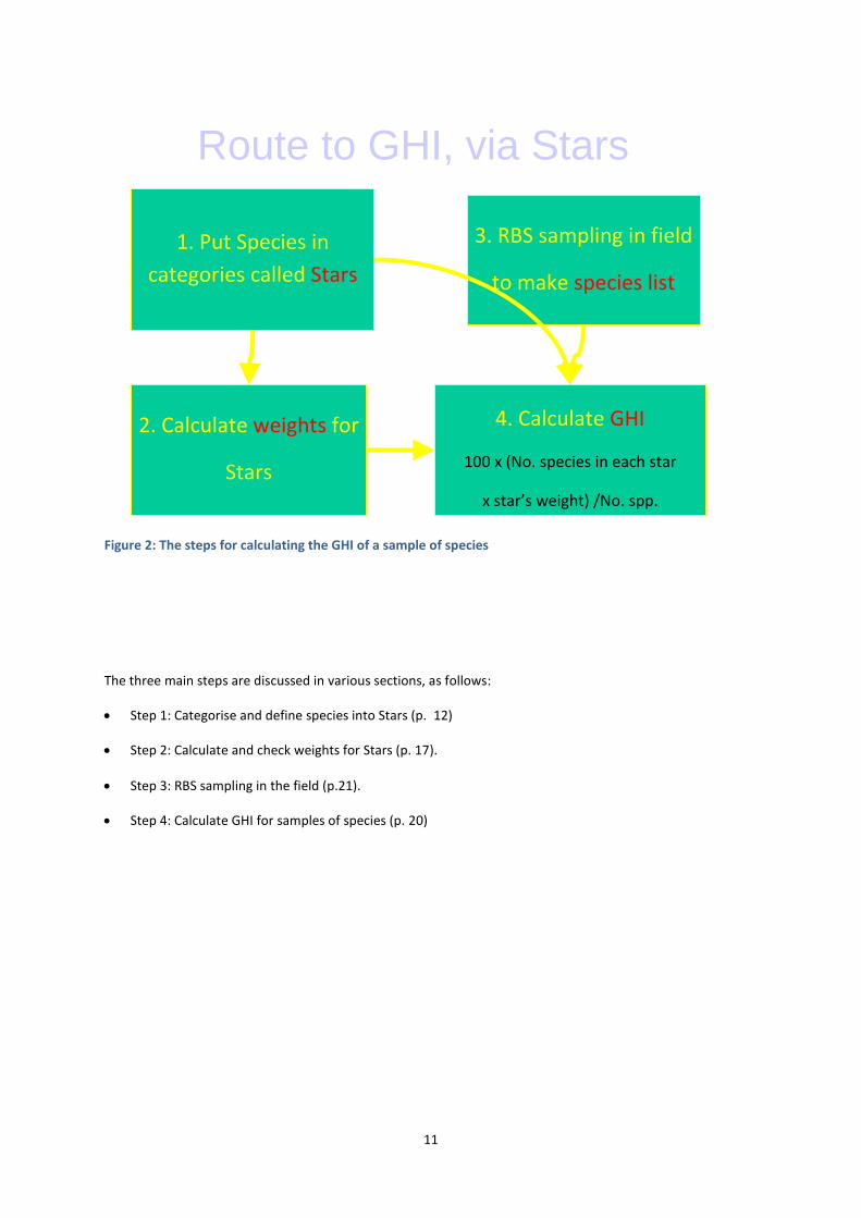
The Genetic Heat Index (GHI) is an index of bioquality for a sample, whether that sample is a single plot, or a
forest or regional checklist. The GHI indicates the chance that a random species from the specified plant
community is a globally rare one – a Black, Gold or Blue Star species - weighted by the degree of global rarity.
To calculate GHI, species are assessed for Global rarity (put into Star categories) using all available data, and
species lists for various community samples are assembled separately, ideally using RBS fieldwork. The spectrum
of different Stars in the samples determines the GHI, The process is shown in Figure 2.
11
The three main steps are discussed in various sections, as follows:
Step 1: Categorise and define species into Stars (p. 12)
Step 2: Calculate and check weights for Stars (p. 17).
Step 3: RBS sampling in the field (p.21).
Step 4: Calculate GHI for samples of species (p. 20)
Route to GHI, via Stars
1. Put Species in
categories called Stars
2. Calculate weights for
Stars
3. RBS sampling in field
to make species list
4. Calculate GHI
100 x (No. species in each star
x star’s weight) /No. spp.
Figure 2: The steps for calculating the GHI of a sample of species
12
STEP 1. CATEGORISE SPECIES INTO STARS
Species are allocated to colour coded categories of global rarity called Stars, based on their global distributions
and, to a lesser extent, taxonomic and ecological rules.
13
Table 2. Global rarity is very much the strongest influence on the Stars allocated to species, but cannot be
considered separately from various other issues.
Black Stars are the top, i.e. rarest, category. At the other extreme, Green Stars are widespread and of no special
conservation concern in terms of their rarity. The sequence from high to low rarity or conservation value is:
Black, Gold, Blue and Green Star1.
In the earliest RBS in Ghana, heavily exploited but globally common species were originally distinguished as
separate Reddish (Scarlet, Red or Pink) Stars (Hawthorne, 2001) depending on how intensively they were
exploited. It is now the standard method to keep the bioquality index simpler and more specifically linked to
global rarity, so all species are defined as Black, Gold Blue or Green Stars, even if heavily exploited. Where global
usage status is well-known, Reddish Stars can be listed alongside, not instead of the four main Star colours (as
with other conservation-related categories, such as IUCN status).
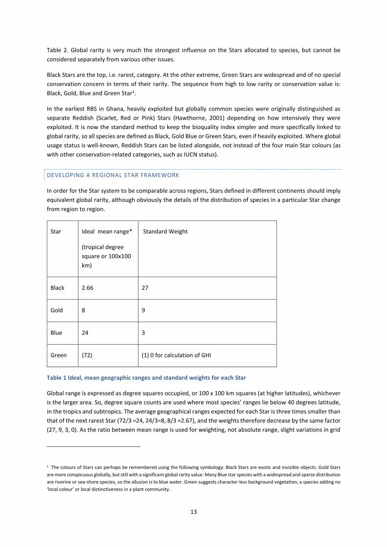
DEVELOPING A REGIONAL STAR FRAMEWORK
In order for the Star system to be comparable across regions, Stars defined in different continents should imply
equivalent global rarity, although obviously the details of the distribution of species in a particular Star change
from region to region.
Star Ideal mean range*
(tropical degree
square or 100x100
km)
Standard Weight
Black 2.66 27
Gold 8 9
Blue 24 3
Green (72) (1) 0 for calculation of GHI
Table 1 Ideal, mean geographic ranges and standard weights for each Star
Global range is expressed as degree squares occupied, or 100 x 100 km squares (at higher latitudes), whichever
is the larger area. So, degree square counts are used where most species’ ranges lie below 40 degrees latitude,
in the tropics and subtropics. The average geographical ranges expected for each Star is three times smaller than
that of the next rarest Star (72/3 =24, 24/3=8, 8/3 ≈2.67), and the weights therefore decrease by the same factor
(27, 9, 3, 0). As the ratio between mean range is used for weighting, not absolute range, slight variations in grid
1 The colours of Stars can perhaps be remembered using the following symbology: Black Stars are exotic and invisible objects. Gold Stars
are more conspicuous globally, but still with a significant global rarity value. Many Blue star species with a widespread and sparse distribution
are riverine or sea-shore species, so the allusion is to blue water. Green suggests character-less background vegetation, a species adding no
‘local colour’ or local distinctiveness in a plant community.

14
system used for counting range in different projects makes no significant difference, especially when one
considers other factors that make any range size estimates imprecise.
The initial goal of Star rating is to estimate degree square (or 100 x 100 km) occupancy for the species of interest.
Increasingly, this can be achieved by using published, digitised distribution data. Digitised distribution data
remain patchy however, so a set of chorological (biogeography-related) rules can also be generated to allow the
botanist to extract information from other sources such as Floras, monographs and biogeographic treatments
of floras, and relate it to the Star categories.
To use digitised distribution data, a species list for the region of interest is required. This species list can be used
to download and compile distribution records for the species. Sources of digital distribution data vary by region,
but are commonly held by regional herbaria, and other herbaria with a history of collection in the region.
Distribution data are also available through GBIF (www.gbif.org). Global distribution data for the species should
be compiled, such that the global ranges of the species can be estimated (e.g. not only records from inside your
region). This degree square occupancy estimate for each species should be referred to when using the regional
framework for Star rating, keeping in mind the typical degree square occupancy suggested for each Star
category. Degree square occupancy estimated in this way should be considered as the minimum occupancy,
unless there is reason to believe that collection and digitisation has been particularly complete for a species. The
Stars are as far as possible standardised globally, and adapted regionally into a regional Star definition
framework. Thus far, regional frameworks have been developed as and when demanded by RBS-related
projects, with separate projects for example covering all of: mainland tropical Africa, Trinidad and Tobago, Japan
and the Brazilian cerrado. Each regional framework is work in progress, the best practicable answer that can be
made at a stated time for a given region. Botanists are encouraged to debate both the definitions for each Star
in the regional framework and the Stars allocated to particular species using these rules, both of which may
change as plant exploration progresses.
The regional framework can be presented as a table or key (see example in Table 3), devised so that:-
It is fairly easy to work out which Star most or all species in the region should be in, at least for a first
approximation, from a summary of the global distribution pattern of the species, for instance from a
published Flora or monograph or distribution data.
The geographic ranges of species placed in the different Stars are significantly different, in terms of the
mean and standard deviation of the geographic range for species in that Star, and are as close as possible
to those defined in Table 1.
The rules are adapted regionally to yield Stars with similar mean geographical range in different regions, so Gold
Star Chilean species, for instance, have an average range that is as close as possible to the Gold Star Ghanaian
species2.
2 Insofar as exact alignment is not possible for the mean ranges of species in a given Star in each region, the
weights for Stars could be fine-tuned within specific projects to reflect their relative rarity more precisely.
However, as the results are of greatest interest when compared globally, we propose to use the same standard
set of weights, as it would make no sense for a Blue, Black or Gold Star species to be weighted differently
depending on region/project of assessment. The actual, statistical difference between the adjusted and default
weight for Stars should in any case be stated when the Star framework is set up.
15
GHI weights for a given Star should always be based on extant facts, referring to all herbarium-based distribution
data for a subset of or all species in the Star, rather than their hypothetical or modelled ranges. However, the
primary categorisation of species into Stars is made practical by considering species range in terms of broad
biogeographical categories, like ‘widespread across tropical Africa’. The framework definition clarifies
specifically what this might mean in terms of distribution patterns (e.g. “one or more records from each of East
Central and West Africa”, or ‘known only from a single Kenya flora district).
The mean range of species in such categories is calculated for a subset of species, those which are more certain
taxonomically and for which the reliable distribution data is available.
16
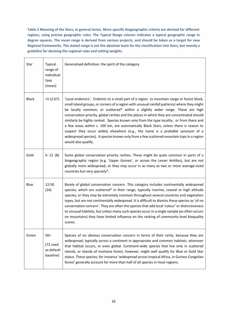
Table 2 Meaning of the Stars, in general terms. More specific biogeographic criteria are devised for different
regions, using precise geographic rules. The Typical Range column indicates a typical geographic range in
degree squares. The mean range is derived from various projects, and should be taken as a target for new
Regional frameworks. The stated range is not the absolute basis for the classification into Stars, but merely a
guideline for devising the regional rules and setting weights.
Star Typical
range of
individual
taxa
(mean)
Generalised definition: the spirit of the category.
Black <5 (2.67). ‘Local endemics’. Endemic to a small part of a region (a mountain range or forest block,
small island groups, or corners of a region with unusual rainfall patterns) where they might
be locally common; or scattered* within a slightly wider range. These are high
conservation priority, global rarities and the places in which they are concentrated should
similarly be highly ranked. Species known only from the type locality, or from there and
a few areas within c. 100 km, are automatically Black Stars, unless there is reason to
suspect they occur widely elsewhere (e.g., the name is a probable synonym of a
widespread species). A species known only from a few scattered mountain tops in a region
would also qualify.
Gold 5- 12 (8) Some global conservation priority rarities. These might be quite common in parts of a
biogeographic region (e.g. ‘Upper Guinea’, or across the Lesser Antilles), but are not
globally more widespread, or they may occur in as many as two or more average-sized
countries but very sparsely*.
Blue 12-50
(24)
Barely of global conservation concern. This category includes continentally widespread
species, which are scattered* in their range, typically riverine, coastal or high altitude
species; or they may be extremely common throughout several countries and vegetation
types, but are not continentally widespread. It is difficult to dismiss these species as ‘of no
conservation concern’. They are often the species that add local ‘colour’ or distinctiveness
to unusual habitats, but unless many such species occur in a single sample (as often occurs
on mountains) they have limited influence on the ranking of community level bioquality
scores.
Green 50+
(72 used
as default
baseline)
Species of no obvious conservation concern in terms of their rarity, because they are
widespread, typically across a continent in appropriate and common habitats, wherever
that habitat occurs, or even global. Continent-wide species that live only in scattered
islands, or islands of montane forest, however, might well qualify for Blue or Gold Star
status. These species, for instance ‘widespread across tropical Africa, in Guineo-Congolian
forest’ generally account for more than half of all species in most regions.
17
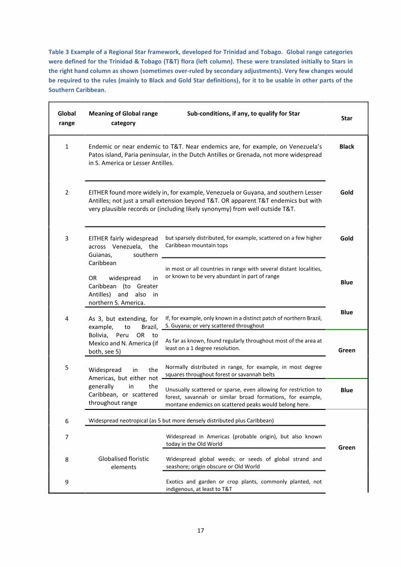
Table 3 Example of a Regional Star framework, developed for Trinidad and Tobago. Global range categories
were defined for the Trinidad & Tobago (T&T) flora (left column). These were translated initially to Stars in
the right hand column as shown (sometimes over-ruled by secondary adjustments). Very few changes would
be required to the rules (mainly to Black and Gold Star definitions), for it to be usable in other parts of the
Southern Caribbean.
Global
range
Meaning of Global range
category
Sub-conditions, if any, to qualify for Star Star
1 Endemic or near endemic to T&T. Near endemics are, for example, on Venezuela’s Patos island, Paria peninsular, in the Dutch Antilles or Grenada, not more widespread in S. America or Lesser Antilles.
Black
2 EITHER found more widely in, for example, Venezuela or Guyana, and southern Lesser Antilles; not just a small extension beyond T&T. OR apparent T&T endemics but with very plausible records or (including likely synonymy) from well outside T&T.
Gold
3
EITHER fairly widespread across Venezuela, the Guianas, southern Caribbean
OR widespread in Caribbean (to Greater Antilles) and also in northern S. America.
but sparsely distributed, for example, scattered on a few higher Caribbean mountain tops
Gold
in most or all countries in range with several distant localities, or known to be very abundant in part of range
Blue
Blue 4 As 3, but extending, for
example, to Brazil, Bolivia, Peru OR to Mexico and N. America (if both, see 5)
If, for example, only known in a distinct patch of northern Brazil, S. Guyana; or very scattered throughout
As far as known, found regularly throughout most of the area at least on a 1 degree resolution. Green
5 Widespread in the Americas, but either not generally in the Caribbean, or scattered throughout range
Normally distributed in range, for example, in most degree squares throughout forest or savannah belts
Unusually scattered or sparse, even allowing for restriction to forest, savannah or similar broad formations, for example, montane endemics on scattered peaks would belong here.
Blue
6 Widespread neotropical (as 5 but more densely distributed plus Caribbean)
Green
7
Globalised floristic elements
Widespread in Americas (probable origin), but also known today in the Old World
8 Widespread global weeds; or seeds of global strand and seashore; origin obscure or Old World
9 Exotics and garden or crop plants, commonly planted, not indigenous, at least to T&T
18
SECONDARY ADJUSTMENTS TO THE STAR FOR A TAXON
Once all species have been allocated a default Star based on geographic range, secondary adjustments – up or
down one or more Stars from that which the regional framework prescribes for the recorded global range– are
allowed for taxa that are judged to be, in effect, more or less globally rare (ecologically or taxonomically) than
normal, providing data are judged to be reliable and according to the following considerations.
Species with unusually scattered distributions within their whole range can be upgraded. Some ‘scattered’
species suggest a relict (once more widespread) distribution; other cases may be due to erratic, long
distance dispersal. In both cases, these species are often associated with specific, scattered habitat e.g.
isolated mountain tops.
Species that tend to regenerate sporadically or occur very sparsely within their range may be upgraded a
Star – if they are deemed to be, in effect, globally more than three times rarer than average for species with
the same range.
Some taxa, like canopy epiphytes and small aquatics, are under-sampled in herbaria compared to terrestrial
shrubs with conspicuous flowers. Classifiers should try to compensate for this, if necessary downgrading
very inconspicuous and significantly under-collected species relative to what the framework suggests, as it
is reasonable to assume that they are commoner than they seem.
Invasives, aggressive pioneers that are naturalised and expanding their range, typically dominant over large
areas, can be downgraded a Star. They are in effected counted as globally less rare than their recorded
range suggests. In practice, most such species are widespread Green Star species even without this
adjustment.
Species that are widely cultivated, such as Coffea spp. should have a lower Star than that implied by the
supposed natural range, when assessing communities where such species are found persisting after, or
escaping from cultivation. It may be appropriate and possible to distinguish escaped cultivars from wild-
type ancestral plants, and score them separately. A separate informal name entry and higher weight Star
can be introduced in the database to designate isolated wild and genetically distinct populations. (‘Coffea
arabica- wild Ethiopian population’, Black Star; vs ‘Coffea arabica (cult.)’, Green Star)
Species very isolated taxonomically from their nearest relative can also be upgraded, e.g. species of mono-
specific genera. Species very dubiously distinct from other species can be downgraded.
In case of doubt, about taxonomy or range, the lower value (commoner option) from a range of Star options
should as a rule be selected. Two very closely related and similar species are more likely to become sunk into
one species by future taxonomists than two distantly related ones: secondary adjustments should help stabilise
the Star assessment in the face of shifting taxonomic opinion.
Consideration of relatedness is justified not only to help stabilise assessments, but also because maintenance of
both inter- and infra- specific genetic diversity globally is an aim of biodiversity conservation, and this is only
partly captured in the formal taxonomy. The global range of taxa, the key criterion for Stars, is not at all
independent of taxonomic opinion and patterns of variation. The importance of this approach becomes more
obvious when one tries to assign Stars to infra-specific taxa.
STARS FOR DIFFERENT TAXONOMIC RANKS & INFLUENCE OF RELATEDENESS
Basic consideration of relatedness between taxa provides a philosophical framework for allocating Stars to infra-
specific taxa: it allows a rationale for varieties and subspecies to be allocated a Star that is different from the
species as a whole. Varieties, sub-species and forms (any infra-specific taxa – VARS below) can have higher, or
the same Star as the species which contains them, for the following reasons.
19
VARS are obviously always rarer globally than the species which includes them, as they are but part of the
whole species. On the other hand, they may be very closely related to other VARS of the same species which
together constitute the full species’ range. It would make little sense if VARS were always higher-ranked on
the basis of this greater rarity. That way we could end up with an illogical situation where two Black Star
varieties constitute a Gold Star species.
Yet, it is not unreasonable that a species as a whole may be lower ranked than SOME of its VARS, e.g., a
Gold Star species composed of one Gold Star and one Black Star variety. This signals uncertainty over which
variety is represented by any record referred to only at the species level. In the face of uncertainty,
bioquality estimates should be conservative, so the Star for a species is always equal to that of its lowest
ranked VAR. It is important to ensure all VARS of the species are considered, not just those from the region
under study, so where some VARS are missing for a species otherwise included in a regional database, the
Star of this species should be set at the default for the total species’ range, pending more detailed
assessment of all missing VARs.
Guidelines for secondary adjustment of Stars based on relatedness can be laid out as follows.
1. First of all calculate the Stars for species as a whole, as if no VARS had ever been published.
2. VARS can never have a lower ranked Star than their species as a whole. By default, all VARS have the
same star as their species, so pending further consideration repeat the species’ Star for all VARS.
3. When adequate data are available, consider the range of each VAR in turn, using the geographic
guidelines as if each was a separate species. The VAR can be upgraded to a maximum of the Star it
would be allocated if it were a separate species, but usually in view of the close relatedness of the VAR
to other VARS it may be appropriate to allocate a Star between this value and that of the whole species.
4. If expert taxonomic opinion shows they are very well defined and distinct VARS, such that other
taxonomists might well have treated them as a different species, prefer the higher ranked Star option.
If the VARS are only subtly different, and have very similar sister VARS that would extend their range
dramatically if considered together, choose the lower option.
5. If a VAR is different in only trivial ways (e.g. only slightly hairier flowers and stems), then be more
disposed to use the same Star as for the species as a whole. Or, if populations of the VAR are more
distinct than usual from the rest of the species, tend towards the Star suggested for the VAR if it were
a distinct species.
6. If the VAR has a particularly narrow range in a distant locality, geographically isolated from the rest of
the species, prefer the higher Star possibilities. If the range overlaps considerably with that of the rest
of the species, maybe enclosed within it and not isolated ecologically, choose the lower option.
7. If all VARS (globally) of a species have been assessed, ensure the species’ Star equals that of the lowest
ranked VAR.
For example:
Begonia quadrialata is widespread across the Guineo-Congolian region.
Begonia quadrialata subsp. quadrialata is widespread in West Africa, and Lower Guinea (to Gabon).
Begonia quadrialata subsp. nimbaensis is endemic to the Nimba mountains of Upper Guinea in an area less
than 50 km wide (in three 0.5 degree square cells, or one 1 degree square – Poorter et al.2004)
First, consider the species as a whole. It is very widespread and common and therefore Green Star. Likewise, the
widespread subsp. quadrialata is Green Star.
If B. quadrialata subsp. nimbaensis were a distinct species, i.e. if it had species status, it would qualify for a Black
Star. If the variety had been very distinct, it might have been kept as a Black Star species, given the very narrow
range, but subsp. nimbaensis is very similar to the other subspecies, and so qualifies as Gold Star at best. In fact,
20
the two subspecies have recently been found growing closely together in intimately mixed colonies on Mt.
Nimba suggesting even slighter genetic differences than previously thought. Knowing this, and that subsp.
nimbaensis could soon be sunk, or reduced to a mere forma, leads us to downgrade it to Blue Star, reflecting
very close affinity to the more widespread form. This has the useful side effect of helping stabilise the GHI of
samples which include it, in the context of future likely taxonomic changes.
So, subsp. nimbaensis is Blue Star, yet the species as a whole is Green Star. i.e. the species as a whole has a lower
rank than one of its subspecies as outlined above, the lowest, more conservative possible interpretation. The
onus is on the botanist to specify the subspecies in these cases. Often the VAR can be deduced from geographic
location of the specimen, so can be applied automatically once the species is determined (but this does not
apply here).
On a slightly different basis, one can sometimes allocate Stars to unidentified specimens of known species in
particular genera, at least within the context of a specific project area. If all species of a genus are Gold Star,
then any unidentified specimen is very likely to be one of them (but unspecified maybe due to lack of flowers)
and can be given a Gold Star in that context. Time spent trying to identifying sterile specimens for bioquality
assessment is reduced if one knows there is no point spending a lot of time deciding which of several species of
a Green star genus one has. This shortcut is not possible if various species from a genus have different Stars.
Tabernaemontana trees in West Africa belong to one of a few widespread (Green Star) and common species, so
unidentified Tabernaemontana trees are also allocated Green Star. This is particularly useful because the species
are common and can usually not be distinguished when infertile.
STEP 2. CHECKING WEIGHTS FOR STARS FROM GLOBAL RANGES
As a draft Star framework is developed, the mean global rarity for each Star is established for a sub-sample of
the species in each Star from recent taxonomic monographs and revisions. It is assessed as the number of degree
squares occupied (or of 100 x 100km grid squares outside the tropics and subtropics where degree squares
become smaller than this area). This is only calculated for a subset of species because, for the majority of species,
detailed degree square distribution maps are usually not available.
The category of the globally commonest species (Green star) is treated as a baseline of zero value, equivalent to
an infinite range, but the value of 72 degree squares is taken as a standard value for the Green Star range, for
weighting purposes. There is little need to calculate this range for many of the Green Star species, except to
check that the concept is correctly applied and that the regional framework leads to Green Stars with a mean
distribution of more than 50 d.s.. Weights for other Stars are calculated based roughly on the inverse mean
global rarity of each Star (rounded to an integer), relative to this baseline, of 72 d.s,. for Green Star.
The aim is that Stars defined in different regions lead to sets of species with similar mean range. The framework
rules for Stars should be adjusted as far as possible to lead to sets of species with the preferred mean range,
although exact alignment is not always possible.
The rarest category - Black Star species – should be defined in a way which means they occupy as close as
possible to 2.7 degree squares on average, as the weight of 27 (72/2.66=27) is used for standard calculation of
GHI.
A standard grid should be specified for any survey, e.g. for tropical regions, the degree square grid with origin at
the equator and the Greenwich meridian. The alignment of the surveyed area with respect to the degree square
grid can influence the weights slightly, particularly for Black Star species. Many species with a narrow range that
could fit in a single degree square have occurrences which straddle the standard latitude and longitude lines,
falling in 2-4 grid cells. It is preferable to keep the range estimates objective rather than trying to minimise ranges
21
by shifting the grid origins for each species, not least because published data usually does not allow such
regridded estimates. In regions where the grid alignment biases the estimated ranges (e.g. with a narrow
mountain range running along a meridian line), a slightly higher than the default mean range (2.7) for Black Star
species is acceptable.
STEP 4. CALCULATE GHI FOR A SAMPLE OF SPECIES
We will describe the RBS field methods below. Even though that is potentially Step 3 in the four step process for
calculating bioquality, there is a lot more to RBS field methodology that needs to be explained. Here, readers
only need note that a RBS sample provides a local list of species, and that a GHI can be calculated from any list
of species. How meaningful the GHI is, though, depends on how the sample was assembled in the first place.
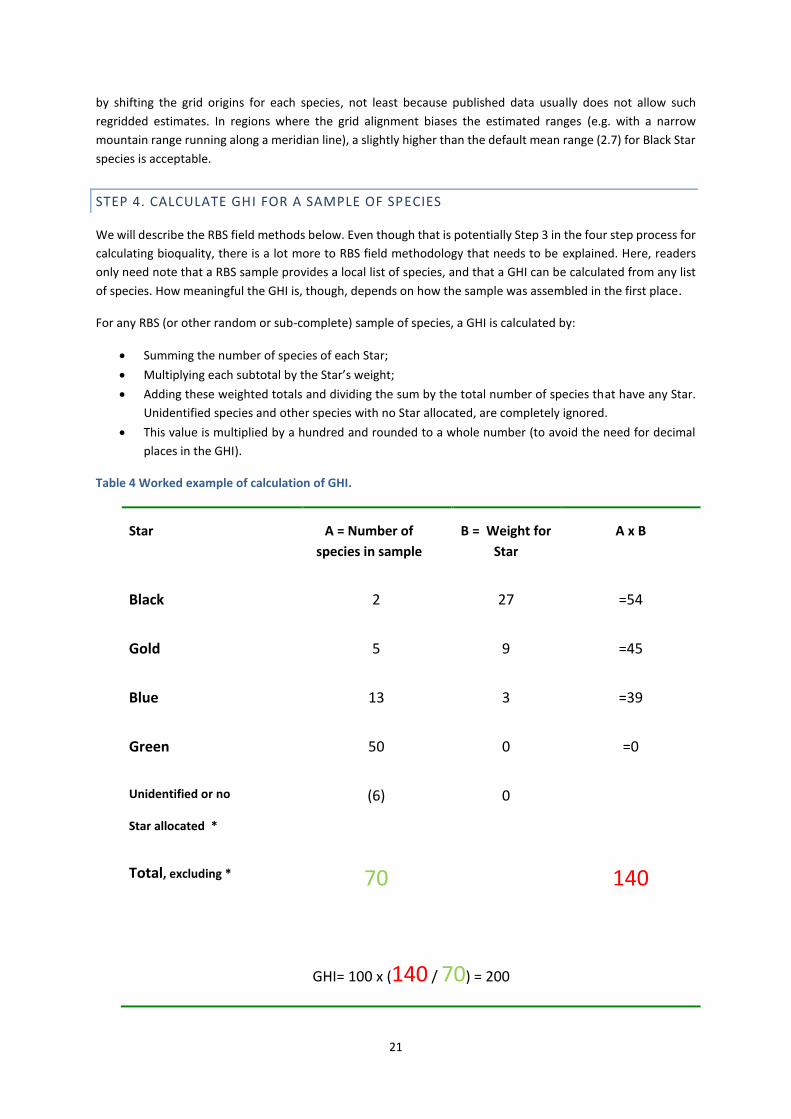
For any RBS (or other random or sub-complete) sample of species, a GHI is calculated by:
Summing the number of species of each Star;
Multiplying each subtotal by the Star’s weight;
Adding these weighted totals and dividing the sum by the total number of species that have any Star.
Unidentified species and other species with no Star allocated, are completely ignored.
This value is multiplied by a hundred and rounded to a whole number (to avoid the need for decimal
places in the GHI).
Table 4 Worked example of calculation of GHI.
Star A = Number of
species in sample
B = Weight for
Star
A x B
Black 2 27 =54
Gold 5 9 =45
Blue 13 3 =39
Green 50 0 =0
Unidentified or no
Star allocated *
(6) 0
Total, excluding * 70 140
GHI= 100 x (140 / 70) = 200
22
RBS SAMPLING IN THE FIELD (STEP 3)
RBS fieldwork is Step 3 out of four key steps defined above for calculating the bioquality across a landscape. RBS
has other uses, apart from bioquality scoring. In this section the RBS field methodology is introduced and
explained, after a recap of generic RBS aims.
SUMMARY OF RBS AIMS
RBS aims, with minimal effort, to provide a rapid, yet penetrating and useful overview of the vascular plant
biodiversity and vegetation in an area, in relation to the landscape, and to provide information on various
aspects of plant distribution, including:
Plant distribution in the surveyed area. RBS helps uncover unknown localities of rare species whilst
paying due attention to the distribution of common ones.
The main trends in vegetation variation and how species are distributed with respect to environmental
variables, especially position in the landscape and disturbance history.
Vegetation bioquality and conservation priority, at the finest scale practical for vascular plants. (See
page 9 for discussion on how RBS can act as a bioquality thermometer.) A key aim of many RBS projects
is to expose and dissect plant bioquality hotspots, employing a particular and precise definition of
biodiversity hotspot, whereby:
the threat factor is excluded from the index of ‘hotspotness’, in contrast to Myers et al. (2000)
where high threat is a necessary condition for a region to be counted as a hotspot;
The GHI can be applied at any scale, so RBS focuses on a fine scale and a bottom-up approach.
RBS outputs, including statistical summaries, bioquality and vegetation maps and annotated check-lists, are also
useful for generating hypotheses on aspects of local ecology and biogeography, which may then be tested by
further RBS sampling or more applied sampling or experiment.
RBS also has the following benefits, which can be considered secondary aims.
RBS provides a context in which groups of botanists, foresters, ecologists, professionals or students, are
in the field together, becoming familiar with the current status of the vegetation and landscape under
investigation. RBS teams therefore learn about botanical and other local issues of relevance to the
management of the vegetation, often whilst working with representatives of the relevant state and
local authorities and communities.
RBS facilitates the flow of relevant botanical information back and forth between local and global levels.
Information collected locally is databased and published globally, if appropriate and ethical, whilst
information from elsewhere flows “back to the roots”. Local participants in RBS teams become
informed about which species are globally rare, useful or otherwise considered valuable elsewhere.
RBS can also facilitate production of field guides or other educational materials.
RBS IN RELATION TO OTHER SAMPLING APPROACHES
Many methods have been used for sampling plant biodiversity, and each has its own strengths and weaknesses.
Three commonly used methods are compared with RBS in Table 5. These are:
23
Herbaria, or rather databases of herbarium collections, can be used to generate samples of plant
biodiversity data for particular places. These can be check-lists of all species ever recorded in given
localities, districts or grid squares, and the sampling “method” is the informal and unplanned
wanderings of plant collectors over the centuries (combined with the database query, if appropriate).
The Gentry type transect method (see Missouri website, 2010) is a record of all plants with stems ≥ 2.5
cm (DBH) along ten 2 x 50 m transects, totalling 1/10 hectare at each site. There have been various
modifications, and many types of small, measured plot that include all, or most plant species that have
similar attributes, so are considered in the same column in Table 5.
The relevé samples associated with the Braun-Blanquet method (Westhoff & van der Maarel, 1978),
which has been the mainstay sample method for continental European phytosociology for almost a
century, are subjectively sited to provide a ‘typical’ sample but are measured plots. The area is chosen
in theory to include all species, so there is a problem in patchy vegetation in maintaining homogeneity
with a square area whilst encompassing all the species. Nevertheless, the result can be similar sample
to RBS, and very similar to an RBS made using the optional measured sample area.
Even before biodiversity survey became an issue, foresters used a wide range of sample plot types for
measuring tree density and size class distribution. These “Classic Forestry” plots normally include only
trees larger than 30 cm DBH, sometimes with a subplot for smaller trees. Although individual trees are
recorded in detail, the rest of the flora is ignored. There is therefore some overlap between the Gentry
and Forestry plots, especially in terms of their measured area and focus on plants with stems above a
certain diameter.
RBS field methods incorporate aspects of ‘classical’ herbarium collecting, ecological sampling and tree inventory.
RBS is a less biased, and more systematic and thorough method for sampling plant communities than casual
herbarium collection but is not as systematic (or random) as most forest inventories and other all-tree
permanent plots used for growth studies.
Plant collectors vary in the amount of information they put on the labels for their herbarium specimens. Some
collectors mention lists of species associated with each collected specimen. For example: “Growing with Ceiba,
Manilkara obovata, Microdesmis and Diospyros with a dense under layer of Olyra latifolia in a shaded gulley”.
It is usually unclear how complete these lists are, and often names are generic, but they are still interesting when
researching the ecology of the species represented by the specimen, and even of some interest when
considering the other species in the list. RBS takes this several steps further, by requiring a thorough listing of
the species in each landscape sub-unit. By altering the pattern of the collection compared to classic herbarium
collections, RBS makes the variation in the vegetation the main focus, and the local check-list becomes the
primary goal of the exercise.
RBS samples themselves are generally unmeasured and plotless, based around a point, and in a patch that
represents a defined position within the spectrum of local vegetation and landscape conditions. As many species
as possible locally, representing a highly representative majority at least, are recorded within the chosen
vegetation type. Ideally, recording continues until no more species can be found easily in the defined area. An
RBS database is a suite of micro-checklists like this, with extra information on the places and species concerned.
Sometimes there are linked photographs and other details for the plants in the plots.
24
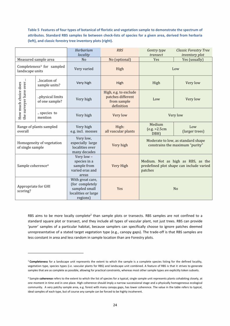
Table 5 Features of four types of botanical of floristic and vegetation sample to demonstrate the spectrum of
attributes. Standard RBS samples lie between check-lists of species for a given area, derived from herbaria
(left), and classic forestry tree inventory plots (right).
Herbarium locality
RBS Gentry type transect
Classic Forestry Tree inventory plot
Measured sample area No No (optional) Yes Yes (usually)
Completeness3 for sampled landscape units
Very varied High
Low
Ho
w m
uch
ch
oic
e d
oes
th
e su
rvey
er h
ave
ov
er…
..location of sample units?
Very high
High
High Very low
..physical limits of one sample?
Very high
High, e.g. to exclude patches different
from sample definition
Low Very low
.. species to mention
Very high Very low
Very low
Range of plants sampled overall
Very high e.g. incl. mosses
High: all vascular plants
Medium (e.g. >2.5cm
DBH)
Low (larger trees)
Homogeneity of vegetation of single sample
Very low, especially large localities over many decades
Very high Moderate to low, as standard shape
constrains the maximum “purity”
Sample coherence4
Very low – species in a
sample from varied eras and
areas
Very High Medium. Not as high as RBS, as the predefined plot shape can include varied patches
Appropriate for GHI scoring?
With great care, (for completely sampled small
localities or large regions)
Yes No
RBS aims to be more locally complete2 than sample plots or transects. RBS samples are not confined to a
standard square plot or transect, and they include all types of vascular plant, not just trees. RBS can provide
‘purer’ samples of a particular habitat, because samplers can specifically choose to ignore patches deemed
unrepresentative of a stated target vegetation type (e.g., canopy gaps). The trade-off is that RBS samples are
less constant in area and less random in sample location than are Forestry plots.
3 Completeness for a landscape unit represents the extent to which the sample is a complete species listing for the defined locality,
vegetation type, species types (i.e. vascular plants for RBS) and landscape unit combined. A feature of RBS is that it strives to generate
samples that are as complete as possible, allowing for practical constraints, whereas most other sample types are explicitly token subsets.
4 Sample coherence refers to the extent to which the list of species for a typical, single sample unit represents plants cohabiting closely, at
one moment in time and in one place. High coherence should imply a narrow successional stage and a physically homogeneous ecological
community. A very patchy sample area, e.g. forest with many canopy gaps, has lower coherence. The value in the table refers to typical,
ideal samples of each type, but of course any sample can be forced to be highly incoherent.
25
RBS is therefore a compromise between the extremes of plant sampling, designed to produce adequately
reliable all-species datasets as rapidly as possible and at a resolution required for documentation and
management of tropical plant biodiversity. RBS does not substitute for other types of plot. Each has a niche of
its own. However, these other types of sample can often be modified to make them compatible with RBS
surveys.
The question has been asked...Why call it ‘Rapid’, when some other methods are faster? The answer is that RBS
achieves a near-complete inventory decades faster than that of casual herbarium collecting (which is compiled
from fertile plants over sporadic visits for many decades). Other fast sampling methods rarely generate such a
complete listing of all plant species, and even if they do, much time is spent on plot demarcation.
RBS AND CLASSICAL HERBARIUM COLLECTIONS
Many of the decisions about plant hotspots and conservation areas have historically been based on a legacy of
herbarium collections, or on the same information published via Floras. Herbaria are essential for ‘getting to
know’ the geographic patterns in a flora, for describing new species and understanding the relationships
between plant groups. They are also essential for identifying collections, such as those produced by RBS itself.
However, herbarium databases are not ideal on their own for spatial assessments of biodiversity on a practical,
local scale. Some of the main differences between casual herbarium and RBS data are:
Herbarium collectors generally target a small subset of the species in the landscape that are fertile at
the time of visiting and considered useful for taxonomic purposes. Often, individual collectors have
their own specific taxonomic group of interest, and it is quite usual that many of the commonest and
most conspicuous plants in a forest at the time of a herbarium collection visit will not be recorded at
all. (If a herbarium collector methodically collected all species and environmental details from discrete,
well-documented, homogeneous sample areas, they would in effect be doing RBS).
RBS surveyors, on the other hand, record as many species as possible – ideally all species regardless of
whether they have flowers or fruits – so that absence of a species’ record from a site at least shows
that it was not obviously present at the time of the survey. At least, no plant species seen in the sample
area are consciously excluded. Inevitably, even RBS surveys miss some species that are ephemeral or
appear seasonally, epiphytes that are far out of reach and (the relatively few) species that are practically
unidentifiable when not flowering, considering the time available for identification. But, there are often
many fewer species missing after a weeks’ work in a suite of RBS samples than following decades of
collecting records for the same, albeit generally more vaguely defined, collecting locality.
Common plants are not recorded in herbaria in proportion to their commonness. Collectors tend to
give up re-collecting very common plants, and even when they are brought in for identification by
amateurs, curators are not inclined to accept all specimens of the commoner species after a certain
number has been included in the herbarium.
Whereas the very common plants that are included tend to be recorded in herbarium databases from
accessible regions closer to herbaria, collectors travelling further from the herbarium on difficult or
expensive field trips often feel disinclined to “waste” their time and luggage or press space with
widespread, common plants when they get there. Thus, we hypothesise that little-visited, remote sites
are more likely to be represented in the herbarium record in a biased way, as if they were
disproportionately rich in rarer species. RBS strictly avoids this “rarer species from remoter places” bias.
Herbarium collectors tend to drift around the landscape and successive records may be from very
different habitats. RBS is focused on creating a complete species list for any sample areas mentioned,
usually one landscape unit at a time.
26
Herbarium locality data tends to be rather imprecise and associated data, e.g. position in landscape,
are recorded inconsistently or not at all by different collectors. These types of metadata are routinely
recorded, and in a consistent way for RBS samples.
Herbarium specimens for a given locality were often collected over a period of many decades, and
species may be absent from the same areas today. RBS is linked to a very short collecting window, so
implications are of known relevance to today’s decisions.
Check-lists for particular areas derived from herbaria are therefore often ‘incoherent ‘ lists of species collected
at a wide range of times, from not very precisely localised areas, e.g. in both wetter and drier sites, with different
levels of attention paid to different plant groups.
In spite of these limitations, herbarium data can still be useful for analysing spatial patterns at a broad spatial
resolution (e.g. for Guyana, Ter Steege et al. 2000; for West Africa Poorter et al., 2005). Surveys at a scale where
individual “samples” have an area of more than 10,000 km2 (roughly, a degree square) are perhaps the most
appropriate use for herbarium data in most countries. The main problem even at this broad scale is that one
can never be confident a priori that the results obtained are truly representative of what is on the ground today.
From the context of herbarium staff, who often form the backbone of RBS teams, RBS gets people into the field,
to see what is happening today and to provide precisely localised snapshots of the biodiversity for this period.
RBS is also typically associated with a period of increased data collation and “cleansing“ of determinations on
old specimens relevant to the survey area, along with a flurry of other beneficial activity in the herbarium. The
RBS snapshots of the plant community can be compared to new samples in subsequent years (or seasons), and
allow surveyors to monitor changes that occur over time with better resolution than if herbarium work had
simply ticked on in the traditional manner, with at best a steady drip of more or less randomly located, fertile
specimens.
In botanically interesting and little-known places, places where RBS is so much needed, RBS teams also select
and photograph the best fertile specimens for herbaria independently of making ecological voucher collections
for the basic RBS.
Typical analyses and outputs and their demands on RBS sampl es
RBS data can be analysed in various ways, but the three most commonly employed types of analysis are:
Ordination or similar multivariate techniques (amply summarised at http://ordination.okstate.edu/).
These provide a neutral, or ‘all species equal’ method to highlight the overall patterns in community
composition across the landscape or through successional change.
Bioquality scoring (p. 10), where all species are weighted by Star categories of global rarity, and a
bioquality score (e.g., GHI) is derived from the array of Stars in each sample.
Species x sampling effort charts, to allow prediction of how many species are likely to be represented
in the whole sampled landscape based on typical rate of expansion of species list for samples to date.
A local species list in the range of 50-150 species is a useful order of sample size for these purposes, depending
on the vegetation being surveyed. The same analyses can also be applied to measured sample plots or even
herbarium locality samples, if various minimum criteria are met. RBS surveys can include measured samples (see
p. 32) to provide extra information.
The shape and extent of plotless RBS samples depends on the shape and extent of landscape subunits, e.g. a
watercourse, defining the sample. It makes little difference to the types of analysis outlined above whether a
27
set of species is from a measured or unmeasured area – they produce compatible results independently of scale.
Smaller samples, and samples following natural boundaries are likely to be more homogeneous and thus can be
more precisely defined ecologically (less blurred or mixed). Therefore indices of the content of small samples,
and of samples with an adaptive shape, can be more extreme in an ordination, than a large sample e.g. a check-
list for a whole forest. However, like a pH value for acidity of a bucket or a cup of water, or a centigrade value
for temperature, the values are not otherwise affected by sample size or shape per se.
RBS data can therefore be analysed and compared with other sample types (e.g. more general check-lists for a
whole forest, or more formal plots) independently of scale, providing the other lists are obtained as effectively
random subsets or as almost complete lists of the same range of species groups (e.g. all vascular plants).
Otherwise, differences in rarity and ecological response shown by different groups of organisms can strongly
bias the results.
Providing the samples have enough species and are not biased by varied taxonomic coverage, results for check-
lists of large areas tend towards the mean or higher end values of the plots within these areas: smaller (RBS
style) samples are more useful for generating means and standard errors rather than a single overall score.
Statistically, many RBS samples for smaller parts of the landscape should have a higher variance of bioquality,
or of ordination score, than fewer larger samples across the same landscape. It is easier to capture smaller
nuances and local facets of the vegetation with smaller plots, but also to pick up uninteresting statistical noise
related to the vagueries of regeneration and random tree-falls.
28
SCOPE, RESOURCES AND THE NUMBER OF SAMPLES IN A SURVEY
An RBS is often project-based, and in any case is best planned as an enterprise of a few months or years. The
scope of an RBS project should be defined with interested parties as concisely as possible, in terms of area on
the map and the precise purpose of the survey. Examples are:
‘to build up a national biodiversity database for our country, to tell us where our plant species live, how
the forest varies and where the plant hotspots are; and as a training ground for student botanists’;
‘as a basis for delimiting plant hotspots precisely and a baseline for future EIAs around our mining
concession to help plan operations in a way that minimises long term impacts to the flora’;
‘as a forum for forestry and the university herbarium to collaborate, especially concerning biodiversity
conservation priorities in the forest reserves’.
A few samples outside the primary scope and theme are useful. For instance, management of a specific forest
or park is often enhanced by gaining more data for species in a few selected areas outside of the boundaries;
and forest management can be improved by samples showing which species regenerate well in fallow outside
the forests.
Usually, one is trying to stretch a limited budget to survey a given area in as much detail as possible. It is advisable
first to estimate how many samples can be completed with the available resources (vehicles, money, staff, and
identification skills). Typical examples of productivity are:
2 RBS samples per day per team is a reasonable rate to expect from a team working in a tropical forest,
reducing to 1 per day where logistics or plant biodiversity make for hard work; and increasing to 3-4
samples per day in species-poor vegetation where access is easy.
A team for a week in the field is about the minimum useful survey effort, yielding 10-20 samples,
suitable perhaps for surveying a single forest patch where the national vegetation pattern and flora is
already fairly well known.
In a team month about 40-60 samples can be completed and these are likely to highlight the major
trends e.g. for a single 30,000 ha forest or small mountain.
It is usually most efficient to plan RBS as a year or longer project, part-time, so that databases can be
optimised in the same period. Over 2 to 4 years, it is possible to complete a survey of all the major
forests of a modest sized country.
o A single team surveyed Ghana’s forest zone, and identified, input and analysed the data for
more than 200 forest reserves, in three years (Hawthorne and Abu Juam, 1995), although
some useful data had been inherited from earlier studies.
o Over 3 years, 250 samples were completed by a team in Trinidad and Tobago, sampling the
islands densely, but intermittently as the team members had other duties in the same period.
Projects with a broader geographical scope tend to have a lower sample intensity. Surveys with thousands of
samples may have to be broken up into smaller themes for analysis anyway. Better then to complete a smaller
survey and, on the basis of the results, survey adjacent areas, or fill in more detail for interesting parts of the
same area.
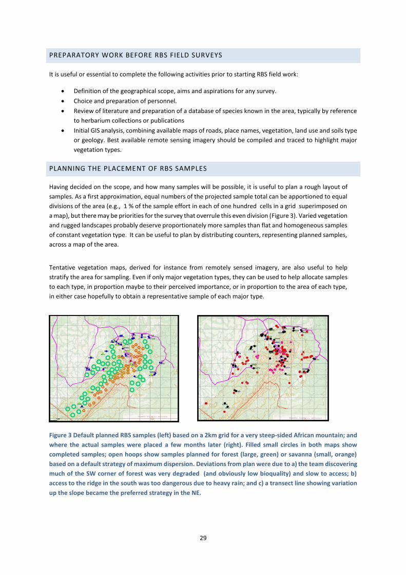
29
PREPARATORY WORK BEFORE RBS FIELD SURVEYS
It is useful or essential to complete the following activities prior to starting RBS field work:
Definition of the geographical scope, aims and aspirations for any survey.
Choice and preparation of personnel.
Review of literature and preparation of a database of species known in the area, typically by reference
to herbarium collections or publications
Initial GIS analysis, combining available maps of roads, place names, vegetation, land use and soils type
or geology. Best available remote sensing imagery should be compiled and traced to highlight major
vegetation types.
PLANNING THE PLACEMENT OF RBS SAMPLES
Having decided on the scope, and how many samples will be possible, it is useful to plan a rough layout of
samples. As a first approximation, equal numbers of the projected sample total can be apportioned to equal
divisions of the area (e.g., 1 % of the sample effort in each of one hundred cells in a grid superimposed on
a map), but there may be priorities for the survey that overrule this even division (Figure 3). Varied vegetation
and rugged landscapes probably deserve proportionately more samples than flat and homogeneous samples
of constant vegetation type. It can be useful to plan by distributing counters, representing planned samples,
across a map of the area.
Tentative vegetation maps, derived for instance from remotely sensed imagery, are also useful to help
stratify the area for sampling. Even if only major vegetation types, they can be used to help allocate samples
to each type, in proportion maybe to their perceived importance, or in proportion to the area of each type,
in either case hopefully to obtain a representative sample of each major type.
Figure 3 Default planned RBS samples (left) based on a 2km grid for a very steep-sided African mountain; and
where the actual samples were placed a few months later (right). Filled small circles in both maps show
completed samples; open hoops show samples planned for forest (large, green) or savanna (small, orange)
based on a default strategy of maximum dispersion. Deviations from plan were due to a) the team discovering
much of the SW corner of forest was very degraded (and obviously low bioquality) and slow to access; b)
access to the ridge in the south was too dangerous due to heavy rain; and c) a transect line showing variation
up the slope became the preferred strategy in the NE.
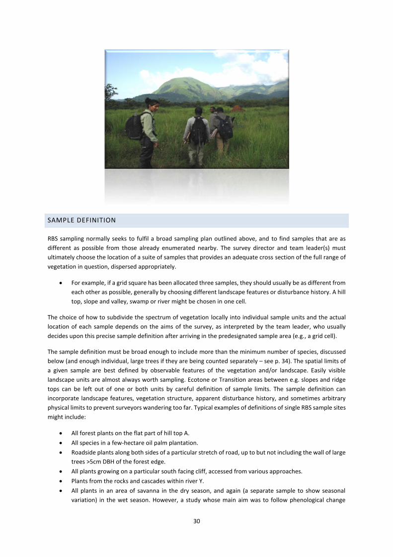
30
SAMPLE DEFINITION
RBS sampling normally seeks to fulfil a broad sampling plan outlined above, and to find samples that are as
different as possible from those already enumerated nearby. The survey director and team leader(s) must
ultimately choose the location of a suite of samples that provides an adequate cross section of the full range of
vegetation in question, dispersed appropriately.
For example, if a grid square has been allocated three samples, they should usually be as different from
each other as possible, generally by choosing different landscape features or disturbance history. A hill
top, slope and valley, swamp or river might be chosen in one cell.
The choice of how to subdivide the spectrum of vegetation locally into individual sample units and the actual
location of each sample depends on the aims of the survey, as interpreted by the team leader, who usually
decides upon this precise sample definition after arriving in the predesignated sample area (e.g., a grid cell).
The sample definition must be broad enough to include more than the minimum number of species, discussed
below (and enough individual, large trees if they are being counted separately – see p. 34). The spatial limits of
a given sample are best defined by observable features of the vegetation and/or landscape. Easily visible
landscape units are almost always worth sampling. Ecotone or Transition areas between e.g. slopes and ridge
tops can be left out of one or both units by careful definition of sample limits. The sample definition can
incorporate landscape features, vegetation structure, apparent disturbance history, and sometimes arbitrary
physical limits to prevent surveyors wandering too far. Typical examples of definitions of single RBS sample sites
might include:
All forest plants on the flat part of hill top A.
All species in a few-hectare oil palm plantation.
Roadside plants along both sides of a particular stretch of road, up to but not including the wall of large
trees >5cm DBH of the forest edge.
All plants growing on a particular south facing cliff, accessed from various approaches.
Plants from the rocks and cascades within river Y.
All plants in an area of savanna in the dry season, and again (a separate sample to show seasonal
variation) in the wet season. However, a study whose main aim was to follow phenological change
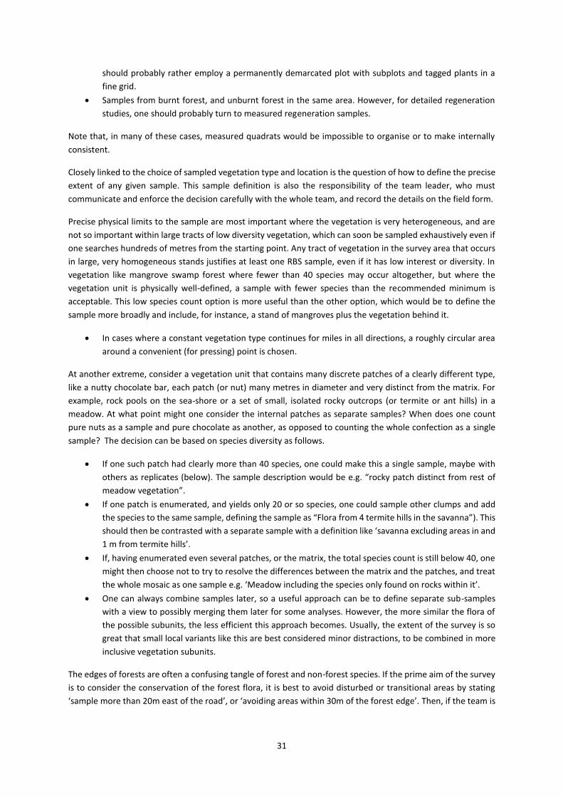
31
should probably rather employ a permanently demarcated plot with subplots and tagged plants in a
fine grid.
Samples from burnt forest, and unburnt forest in the same area. However, for detailed regeneration
studies, one should probably turn to measured regeneration samples.
Note that, in many of these cases, measured quadrats would be impossible to organise or to make internally
consistent.
Closely linked to the choice of sampled vegetation type and location is the question of how to define the precise
extent of any given sample. This sample definition is also the responsibility of the team leader, who must
communicate and enforce the decision carefully with the whole team, and record the details on the field form.
Precise physical limits to the sample are most important where the vegetation is very heterogeneous, and are
not so important within large tracts of low diversity vegetation, which can soon be sampled exhaustively even if
one searches hundreds of metres from the starting point. Any tract of vegetation in the survey area that occurs
in large, very homogeneous stands justifies at least one RBS sample, even if it has low interest or diversity. In
vegetation like mangrove swamp forest where fewer than 40 species may occur altogether, but where the
vegetation unit is physically well-defined, a sample with fewer species than the recommended minimum is
acceptable. This low species count option is more useful than the other option, which would be to define the
sample more broadly and include, for instance, a stand of mangroves plus the vegetation behind it.
In cases where a constant vegetation type continues for miles in all directions, a roughly circular area
around a convenient (for pressing) point is chosen.
At another extreme, consider a vegetation unit that contains many discrete patches of a clearly different type,
like a nutty chocolate bar, each patch (or nut) many metres in diameter and very distinct from the matrix. For
example, rock pools on the sea-shore or a set of small, isolated rocky outcrops (or termite or ant hills) in a
meadow. At what point might one consider the internal patches as separate samples? When does one count
pure nuts as a sample and pure chocolate as another, as opposed to counting the whole confection as a single
sample? The decision can be based on species diversity as follows.
If one such patch had clearly more than 40 species, one could make this a single sample, maybe with
others as replicates (below). The sample description would be e.g. “rocky patch distinct from rest of
meadow vegetation”.
If one patch is enumerated, and yields only 20 or so species, one could sample other clumps and add
the species to the same sample, defining the sample as “Flora from 4 termite hills in the savanna”). This
should then be contrasted with a separate sample with a definition like ‘savanna excluding areas in and
1 m from termite hills’.
If, having enumerated even several patches, or the matrix, the total species count is still below 40, one
might then choose not to try to resolve the differences between the matrix and the patches, and treat
the whole mosaic as one sample e.g. ‘Meadow including the species only found on rocks within it’.
One can always combine samples later, so a useful approach can be to define separate sub-samples
with a view to possibly merging them later for some analyses. However, the more similar the flora of
the possible subunits, the less efficient this approach becomes. Usually, the extent of the survey is so
great that small local variants like this are best considered minor distractions, to be combined in more
inclusive vegetation subunits.
The edges of forests are often a confusing tangle of forest and non-forest species. If the prime aim of the survey
is to consider the conservation of the forest flora, it is best to avoid disturbed or transitional areas by stating
‘sample more than 20m east of the road’, or ‘avoiding areas within 30m of the forest edge’. Then, if the team is
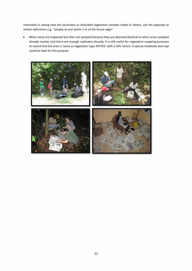
32
interested in seeing how the secondary or disturbed vegetation samples relate to others, use the opposite or
similar definitions e.g. “sample at and within 1 m of the forest edge”.
When areas are inspected but then not sampled because they are deemed identical to other areas sampled
already nearby, and there are enough replicates already, it is still useful for vegetation mapping purposes
to record that the area is ‘same as vegetation type XXYY01’ with a GPS record. A special notebook and map
could be kept for this purpose.
33
REPLICATE SAMPLES
Samples should be repeated in the same vegetation types, but spread across the surveyed area. A good cross-
section of the vegetation will require sufficient and well-dispersed replicates of samples in each of the various
types of vegetation, so team leaders need to be observant, to anticipate what the main types are likely to be,
following analysis. Samples of the same vegetation types across the map help the mapping of vegetation types,
by interpolation or other GIS techniques. Once grouped into formal vegetation types following an ordination or
classification, the different samples of the same type can be used to show statistics of variation for each type,
across the landscape.
Samples in the same, perceived vegetation type in other grid cells should suffice for these aims if the strategy is
using a fine grid to encourage dispersed samples; an equivalent arrangement of samples can also be enforced
without a specific grid.
Some samples can also be repeated in exactly the same sample sites, for various reasons.Replicate samples in
the same exact location but during different seasons could be used to control for effects of season on sample
results, especially in highly seasonal vegetation like deciduous forests and savanna. Return visits could be used
to compile separate sample lists. These could then be merged to form a single sample of that place, for most
analyses. If only a single all-season sample is needed for the site, only new records need strictly be added at the
later visits, but this is then not a replicate, and it may be difficult to remember what was sampled there
previously, so a complete new sample is often the best choice.
Also, samples can be repeated for the same locations by the same or different teams on different occasions, to
test team reliability, or the reliability of the results in general. Replicate samples by the same team in the same
place are best done during the same season, but at least several days apart, as it can be easy to forget which
species are already recorded for a sample if one has collected there recently. These separate enumerations of
the same area can then be included in the same analyses – hopefully the inevitable variation between
enumerations is much smaller than the variation between different samples.
It is best to arrange for two samples enumerated by the same team on the same day to be as different in
species composition as practical.
OPTIONAL MEASURED RBS SAMPLE AREAS (PLOTS)
Samples of a measured size, i.e. orthodox plots, can be included as RBS samples, if the surveyor wants to
calibrate the species richness (or strict species-area curves) for given vegetation types. Another potential role
for measured RBS plots is to act as more tightly controlled, standard sized samples, when a formal vegetation
classification is being defined. Measured plots can provide data that are compatible with RBS data from
unmeasured samples, but involve more work to obtain the same sized species list.
For instance, for forests in Ghana, 20 or 25m square plots have proved adequate for this purpose, optionally
broken into 5 strips, which might be end to end (along a road or river) or side-by-side in a square. These can
provide data on number of species per unit area that is not obtainable from unmeasured RBS samples. In one
survey, a measured subplot was included within a normal RBS sample area. Each sample started with a full
enumeration of a 20 x 20m plot. On completion, a line was drawn on the field sheet and further species records
from the surrounding habitat were added, as for a standard RBS. Trees above 5 cm were enumerated in the
small plot only, and a separate tally of 30+ cm trees was made for the RBS as a whole (30+ cm DBH tree stems
in the measured subplot were flagged as belonging to both sample units).
34
Whilst collection of this additional measured plot data is often of modest extra value, it is often unachievable
for certain vegetation subunits (e.g. cliffs), and may require an extra hour per sample point than an RBS plot
with the equivalent species list. It may be of greatest value in herbaceous vegetation where enforced, closer
scrutiny of the ground layer could be a helpful discipline.
WHAT TO RECORD IN EACH RBS SAMPLE?
As described above, for a single RBS sample, a landscape unit or other well-defined vegetation unit is chosen by
the team leader, depending on both the general scope and plans and opportunistically, based on what is found
on the ground. Then, over a few hours, as many plant species as possible – ideally all of the vascular plant species
that occur there - are recorded. For less well known and diverse vegetation, this should involve collecting most
or all records as specimens, rather than as observations. Each species from the plot need only be pressed once,
and it is up to the booker to decide whether or not the species has already been pressed, with the default being
to collect more rather than less. When a species is pressed and recorded on the form, it is not necessary for the
booker to know its full scientific name, but short or useful names should be given to help keep track. Often, most
of the specimens collected are sterile and a large part of the operation and skill required is concerned with
organising and ultimately identifying these specimens, often by reference to a herbarium.
As a rule of thumb, a single RBS sample should yield more than 40 named species and not take more than 3
sampling hours, but the more species that are recorded the better, providing one does not sample outside the
defined vegetation unit. Also, it is often the case for an efficient team in some vegetation types that after 2
hours, the species list for the sampled vegetation unit has been exhausted in that area.
Typically, 50-150 species are in fact recorded in rain forest RBS samples, but savanna and other
vegetation types may yield only 20-50 species in some localities, if that is the limit of the local diversity.
A complete species list for a sampled area of vegetation is very desirable, and should be the default aim for any
sample, but this is not absolutely essential providing either more than 40 species can be identified in a sample
before analysis, or almost all the species (more than 95%) are collected or recorded. Around and beyond 40
species, extra species records influence community scores only marginally, but do allow greater statistical
confidence, and any records of extra species for the sample area are of course always valuable for distribution
maps drawn from the data.
Data can in any case be statistically rarefied, or reduced to a standard “40 random species” per sample where
needed. Mean and associated error values are, however, normally generated in respect of variation across
individual sample scores (all species) within a given landscape unit (e.g. values for different plots in forest of a
given altitude band).
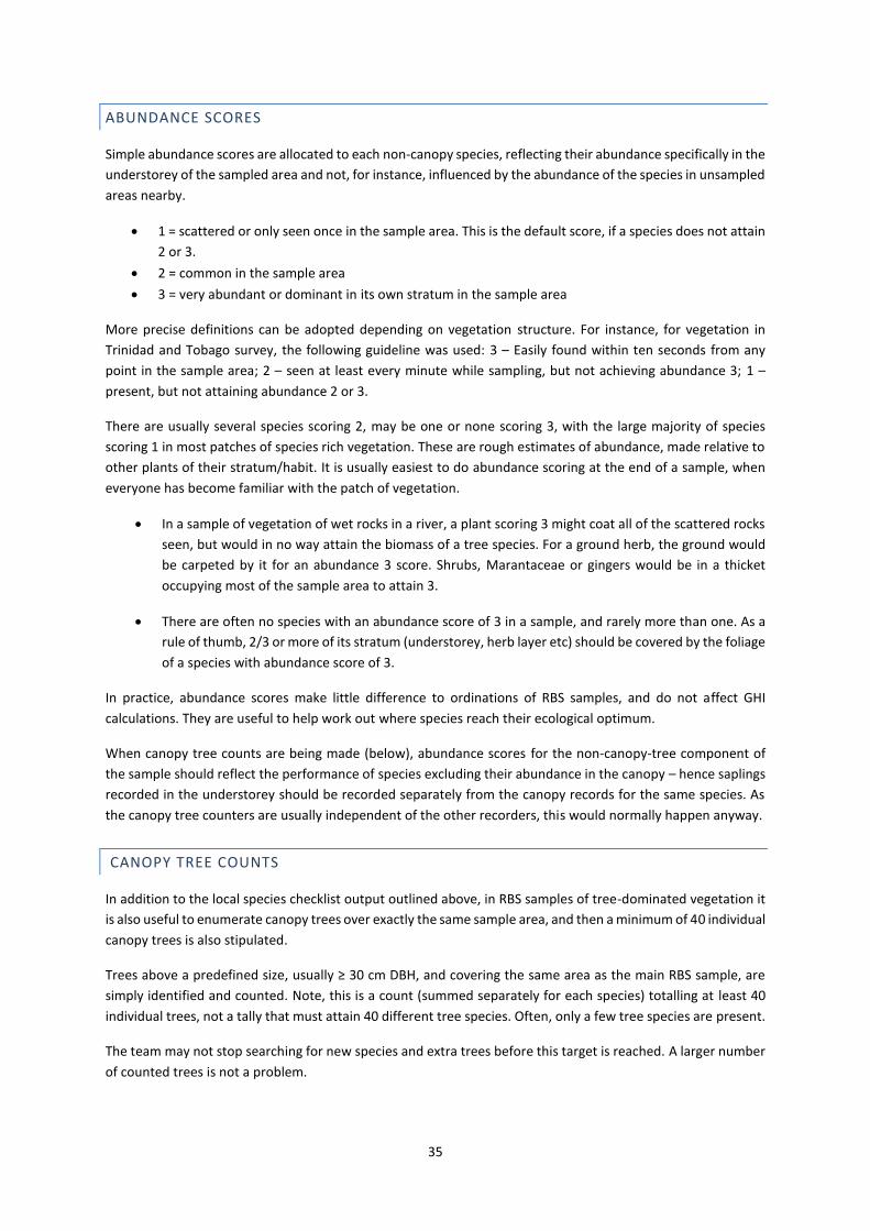
35
ABUNDANCE SCORES
Simple abundance scores are allocated to each non-canopy species, reflecting their abundance specifically in the
understorey of the sampled area and not, for instance, influenced by the abundance of the species in unsampled
areas nearby.
1 = scattered or only seen once in the sample area. This is the default score, if a species does not attain
2 or 3.
2 = common in the sample area
3 = very abundant or dominant in its own stratum in the sample area
More precise definitions can be adopted depending on vegetation structure. For instance, for vegetation in
Trinidad and Tobago survey, the following guideline was used: 3 – Easily found within ten seconds from any
point in the sample area; 2 – seen at least every minute while sampling, but not achieving abundance 3; 1 –
present, but not attaining abundance 2 or 3.
There are usually several species scoring 2, may be one or none scoring 3, with the large majority of species
scoring 1 in most patches of species rich vegetation. These are rough estimates of abundance, made relative to
other plants of their stratum/habit. It is usually easiest to do abundance scoring at the end of a sample, when
everyone has become familiar with the patch of vegetation.
In a sample of vegetation of wet rocks in a river, a plant scoring 3 might coat all of the scattered rocks
seen, but would in no way attain the biomass of a tree species. For a ground herb, the ground would
be carpeted by it for an abundance 3 score. Shrubs, Marantaceae or gingers would be in a thicket
occupying most of the sample area to attain 3.
There are often no species with an abundance score of 3 in a sample, and rarely more than one. As a
rule of thumb, 2/3 or more of its stratum (understorey, herb layer etc) should be covered by the foliage
of a species with abundance score of 3.
In practice, abundance scores make little difference to ordinations of RBS samples, and do not affect GHI
calculations. They are useful to help work out where species reach their ecological optimum.
When canopy tree counts are being made (below), abundance scores for the non-canopy-tree component of
the sample should reflect the performance of species excluding their abundance in the canopy – hence saplings
recorded in the understorey should be recorded separately from the canopy records for the same species. As
the canopy tree counters are usually independent of the other recorders, this would normally happen anyway.
CANOPY TREE COUNTS
In addition to the local species checklist output outlined above, in RBS samples of tree-dominated vegetation it
is also useful to enumerate canopy trees over exactly the same sample area, and then a minimum of 40 individual
canopy trees is also stipulated.
Trees above a predefined size, usually ≥ 30 cm DBH, and covering the same area as the main RBS sample, are
simply identified and counted. Note, this is a count (summed separately for each species) totalling at least 40
individual trees, not a tally that must attain 40 different tree species. Often, only a few tree species are present.
The team may not stop searching for new species and extra trees before this target is reached. A larger number
of counted trees is not a problem.
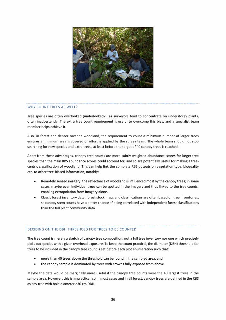
36
WHY COUNT TREES AS WELL?
Tree species are often overlooked (underlooked?), as surveyors tend to concentrate on understorey plants,
often inadvertently. The extra tree count requirement is useful to overcome this bias, and a specialist team
member helps achieve it.
Also, in forest and denser savanna woodland, the requirement to count a minimum number of larger trees
ensures a minimum area is covered or effort is applied by the survey team. The whole team should not stop
searching for new species and extra trees, at least before the target of 40 canopy trees is reached.
Apart from these advantages, canopy tree counts are more subtly weighted abundance scores for larger tree
species than the main RBS abundance scores could account for, and so are potentially useful for making a tree-
centric classification of woodland. This can help link the complete RBS outputs on vegetation type, bioquality
etc. to other tree-biased information, notably:
Remotely sensed imagery: the reflectance of woodland is influenced most by the canopy trees; in some
cases, maybe even individual trees can be spotted in the imagery and thus linked to the tree counts,
enabling extrapolation from imagery alone.
Classic forest inventory data: forest stock maps and classifications are often based on tree inventories,
so canopy stem counts have a better chance of being correlated with independent forest classifications
than the full plant community data.
DECIDING ON THE DBH THRESHOLD FOR TREES TO BE COUNTED
The tree count is merely a sketch of canopy tree composition, not a full tree inventory nor one which precisely
picks out species with a given overhead exposure. To keep the count practical, the diameter (DBH) threshold for
trees to be included in the canopy tree count is set before each plot enumeration such that:
more than 40 trees above the threshold can be found in the sampled area, and
the canopy sample is dominated by trees with crowns fully exposed from above.
Maybe the data would be marginally more useful if the canopy tree counts were the 40 largest trees in the
sample area. However, this is impractical, so in most cases and in all forest, canopy trees are defined in the RBS
as any tree with bole diameter ≥30 cm DBH.
37
Various extra rules can be useful for refining the link between understorey and canopy components of
the sample, at the discretion of the team leader. For instance, along narrow streams, where a stream
canopy tree may be sparser than in normal forest and rooted at some distance from the rest of the
sampled stream flora, an additional horizontal or vertical distance can be applied by the surveyor within
which the canopy trees must be rooted to be included. For instance, this threshold might be up to 5m
from the water edge for the trees and maybe only 1 or 2 m for the lower vegetation. The limit should
be chosen, depending on typical bank steepness, so that the resulting tree sample can exceed 40
individuals whilst still being the canopy of the stream basin; the understorey and canopy limits should
both be narrow enough to reflect a special stream flora within them, if this is what the sample is
designed to detect. These two distances should be documented on the plot description in the field
form.
Obviously if the area is grassland with only a few scattered large trees, the count is of little value and
can be dropped. These samples will not feature in tree canopy analyses. In savanna woodland or
thickets where the canopy is low (and often broken), and too few trees reach 30 cm DBH, the limit can
be lowered to 20, 10 or even 5 cm DBH, a fact which is recorded with the field data, so such samples
can be filtered from analyses if desired. It is best in the survey as a whole to adopt at most only one
other such threshold apart from 30 cm DBH so results are comparable.
Likewise, in more sparsely wooded or disturbed vegetation, a more lenient definition of DBH can be
taken – e.g. to include leaning or forked trees where the lower diameter exceeds the limit even if the
diameter at 1 .3 m vertically above the ground is not strictly so.
As with species records, more than 40 trees can be counted and the extra data are useful. Where this is so, the
tree data can still be analysed alone, with abundance standardised to a proportion of the total tree count, or
rarefied on the computer to yield 40 randomly chosen trees for a given analysis.
RELATING GENERAL ABUNDANCE AND TREE COUNT DATA
When trees are being counted separately, the normal RBS abundance score (1-3) explicitly excludes the canopy
trees, and rather reflects understorey abundance, so the abundance and tree count scores returned from the
field are independent of each other. However, for all-species ordinations and other all-species analyses weighted
by abundance, the overall abundance score for species in the plots should be adjusted to include both strata. A
reasonable conversion rate from tree counts to abundance scores is as follows:
Canopy abundance score 1 = Up to a third (33.33%) of all canopy trees counted.
Canopy abundance score 2 = One third up to two thirds of all canopy trees.
Canopy abundance score 3 = Two thirds or more of canopy trees counted.
The species abundance in the sample as a whole is then taken for analysis as the higher of the two scores, i.e.
observed non-canopy abundance and calculated canopy tree abundance scores.
38
RECORDING LOCAL PERCEPTIONS OF VEGETATION WITH RBS
Assessment of local usage and valuation of plant resources has been integrated into the RBS process. Local
botanical experts are included in RBS teams, and with their help it is a relatively simple matter to collect basic
ethnobotanical data, such as local names and priority species, alongside normal RBS activities. Ethnobotanic
data collected as part of RBS can be used to provide evidence of the cultural and provisioning aspect of
ecosystem services, and allows the differing values attached to biodiversity and ecosystem services by
communities to be accounted for; these elements are considered best practise for ESIAs. Nationally or regionally,
these data could be used to flag dwindling resources and prioritise support, or simply to record how people are
using plants.
HOW DOES IT WORK?
1. Recruiting informants: At the beginning of the field work, the local people who know the most about
the local vegetation are identified through community consultations. Typically, one or two local experts
(e.g. a woman and a man) would accompany an RBS team at a time, but in each community or subset
of communities different local experts can be recruited to reduce individual bias.
2. What is recorded: The local experts accompany the team to the field, and for each specimen collected,
gives their name for the species, how they use it, and how important it is to their community (using a
1-3 score). Use notes are kept perfunctory, e.g. ‘medicine for toothache’, and preparation details are
not requested; this protects the knowledge of local experts whilst providing enough relevant
information for most applications. For canopy tree species, the informant who knows the most about
trees should accompany the tree spotters.
3. Importance scoring: similar in philosophy and execution to abundance scoring, where species receive a
score of 1 by default (‘useful’); 2 for species that are more valued than average; and 3 for the very most
useful species from the sample. Sometimes, no species in a sample will achieve a 3, sometimes several
will, depending on the vegetation. It is usually easiest to do this exercise after all names and specimens
have been recorded.
4. Workshops: Species identified as the most important through the 1-3 scoring can be discussed in
greater detail with the communities. Typical questions would be: Is there enough of this plant around?
Do you have any experience cultivating it? What could be done to improve the supply of this species?
5. Outputs and analysis:
A lexicon of local names and the scientific species to which they correspond. This activity is
greatly facilitated by the collection of many specimens: it is possible to ‘weed out’ incorrectly
named plants, and it becomes clear when a local name corresponds to several scientific
species, or when two local names cover the same scientific species. This becomes very useful
during the management stage, because it means that local people, scientists and managers
can communicate about plant resources.
A summary of how people use plants locally. Plant uses are summarised into use categories,
such as ‘food’, ‘medicine’, ‘magic’, ‘materials’; the numbers of species used for each
application are presented, with example uses detailed.
A list of the most important species locally, with notes about their supply and how they are
currently managed.
An analysis showing to what extent local valuations correspond to global (bioquality) values,
for which species and plant communities these two valuations diverge, and for local
applications, a management plan that takes account of both areas of high bioquality and high
local use value.
6. Follow up work: The data and outputs can form the basis for follow-up surveys conducted by specialists
rather than botanists e.g. market surveys, detailed studies of the customs and rituals linked to plants;
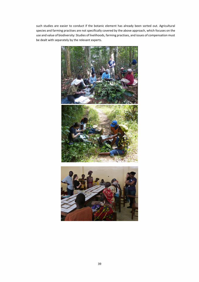
39
such studies are easier to conduct if the botanic element has already been sorted out. Agricultural
species and farming practises are not specifically covered by the above approach, which focuses on the
use and value of biodiversity: Studies of livelihoods, farming practises, and issues of compensation must
be dealt with separately by the relevant experts.
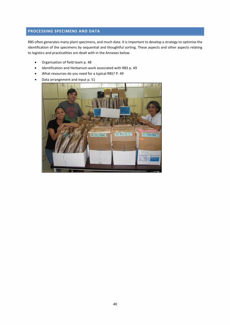
40
PROCESSING SPECIMENS AND DATA
RBS often generates many plant specimens, and much data. It is important to develop a strategy to optimise the
identification of the specimens by sequential and thoughtful sorting. These aspects and other aspects relating
to logistics and practicalities are dealt with in the Annexes below.
Organisation of field team p. 48
Identification and Herbarium work associated with RBS p. 49
What resources do you need for a typical RBS? P. 49
Data arrangement and input p. 51
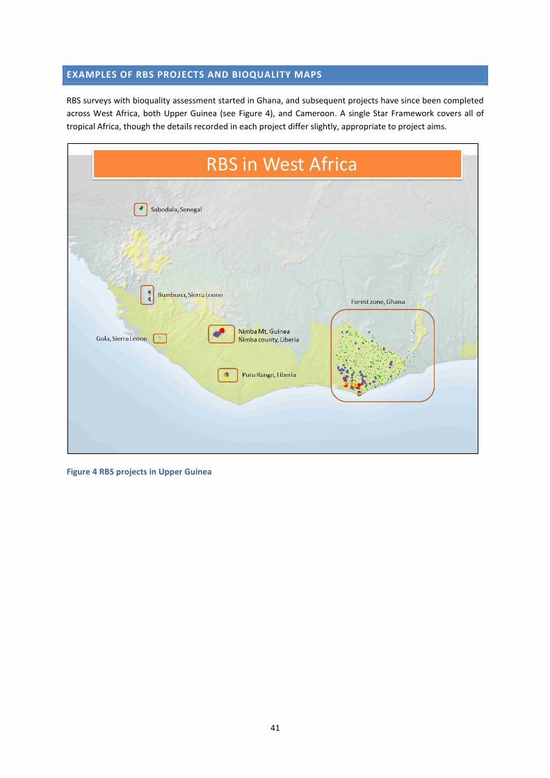
41
EXAMPLES OF RBS PROJECTS AND BIOQUALITY MAPS
RBS surveys with bioquality assessment started in Ghana, and subsequent projects have since been completed
across West Africa, both Upper Guinea (see Figure 4), and Cameroon. A single Star Framework covers all of
tropical Africa, though the details recorded in each project differ slightly, appropriate to project aims.
Figure 4 RBS projects in Upper Guinea
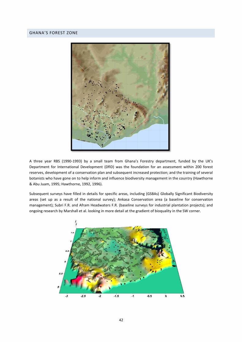
42
GHANA’S FOREST ZONE
A three year RBS (1990-1993) by a small team from Ghana’s Forestry department, funded by the UK’s
Department for International Development (DfID) was the foundation for an assessment within 200 forest
reserves, development of a conservation plan and subsequent increased protection; and the training of several
botanists who have gone on to help inform and influence biodiversity management in the country (Hawthorne
& Abu Juam, 1995; Hawthorne, 1992, 1996).
Subsequent surveys have filled in details for specific areas, including (GSBAs) Globally Significant Biodiversity
areas (set up as a result of the national survey); Ankasa Conservation area (a baseline for conservation
management); Subri F.R. and Afram Headwaters F.R. (baseline surveys for industrial plantation projects); and
ongoing research by Marshall et al. looking in more detail at the gradient of bioquality in the SW corner.
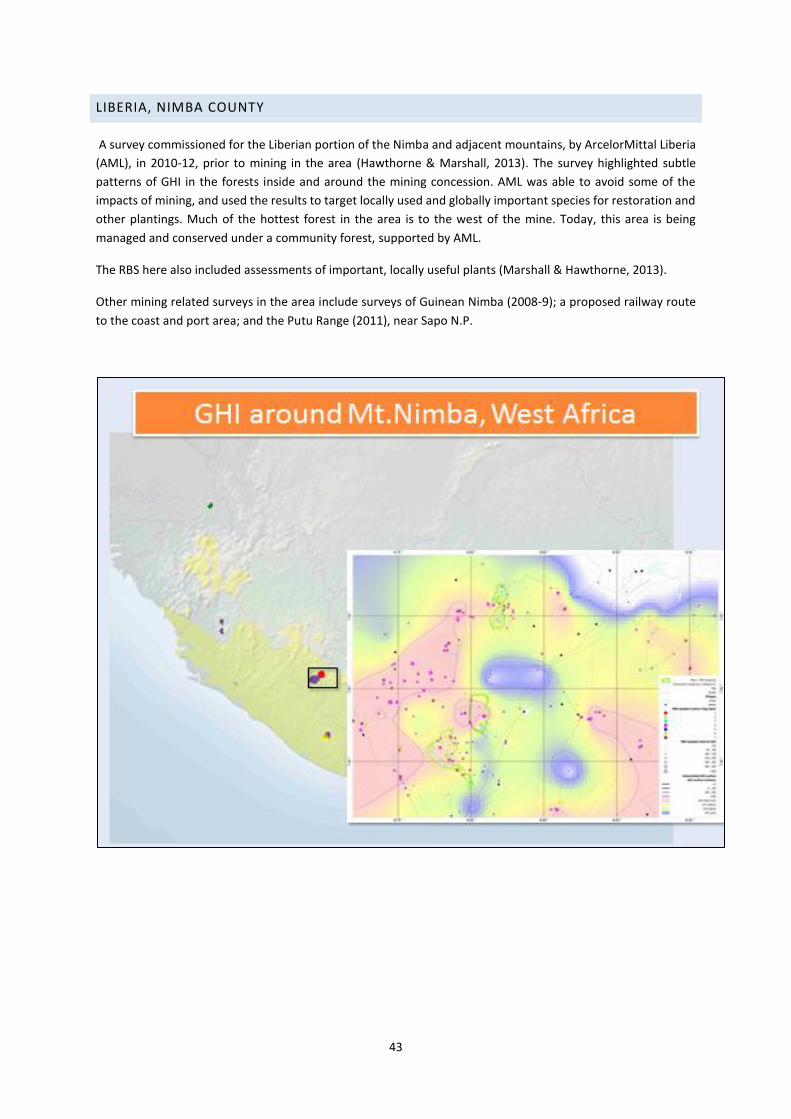
43
LIBERIA, NIMBA COUNTY
A survey commissioned for the Liberian portion of the Nimba and adjacent mountains, by ArcelorMittal Liberia
(AML), in 2010-12, prior to mining in the area (Hawthorne & Marshall, 2013). The survey highlighted subtle
patterns of GHI in the forests inside and around the mining concession. AML was able to avoid some of the
impacts of mining, and used the results to target locally used and globally important species for restoration and
other plantings. Much of the hottest forest in the area is to the west of the mine. Today, this area is being
managed and conserved under a community forest, supported by AML.
The RBS here also included assessments of important, locally useful plants (Marshall & Hawthorne, 2013).
Other mining related surveys in the area include surveys of Guinean Nimba (2008-9); a proposed railway route
to the coast and port area; and the Putu Range (2011), near Sapo N.P.

44
TRINIDAD AND TOBAGO
This three year project involved the University of the West Indies, Forestry Dept. of Trinidad & Tobago and the
University of Oxford, as well as various NGOS. It was funded by the UK government/DEFRA, though the Darwin
Initiative. A bioquality framework was established for the whole country, including a generalized hotspot map,
using RBS samples and the existing herbarium database. The project updated the national flora database, trained
students and foresters, and the data contribute to forest and conservation policy and planning. As well as the
globally significant hotspots detected in the mountains of both Trinidad and Tobago, warm spots (GHI 150-250)
are located on the foothills of these mountains and in other areas to the south and east, and in the small islands
in north west Trinidad.
Yellow and red areas indicate high bioquality areas, measured with the GHI. These areas contain high
concentrations of rare plants and demand the most conservation attention. Ideally, these areas should be
avoided during development and exploitation activities. If they cannot be avoided, they set a baseline against
which restoration or offset activities can be measured. The RBS database was also used in a study of potential
future impacts of climate change in the country (Maharaj, 2012)
Figure 5 Bioquality hotspot map, Trinidad and Tobago. Peaks of GHI in red (at higher altitudes).
45
CLIENTS AND PARTNERS
Our previous clients and sponsors include government departments, industry, charities and NGOs.
Government Departments:
Forestry Departments of Ghana, Liberia, Trinidad & Tobago, Brunei.
UK’s DFID; DEFRA (Darwin Initiative)
Forestry & Wildlife division, Government of Ghana
Add in Cameroon?
Mining and Natural Resources Industry:
BP Biofuels (Brazil)
BHP Billiton; ArcelorMittal Liberia; SMFG (Guinea); Oromin (Senegal); Putu Iron Ore; Euronimba (Liberia)
Bumbuna dam Hydroelectric Power Scheme (Sierra Leone)
Commonwealth Development Corporation (Mt. Cameroon; Ghana Plantations).
Subri Industrial Plantations Ltd (Ghana)
Universities, NGOs and charities:
RSPB/Birdlife International
Kew Millennium Seed Bank
University of the West Indies, St.Augustine, Trinidad & Tobago
University of Talca, Maule Region, Chile
FOR MORE INFORMATION
Contact [email protected]
Office phone: 01865 275 836
46
REFERENCES
Allaby M. 1998, Oxford Dictionary of Ecology. Oxford University Press. Oxford
Baksh-Comeau, Yasmin S., Shobha S. Maharaj, C. Dennis Adams, Stephen A. Harris, Denis L. Filer, and William D. Hawthorne.
2016. An Annotated Checklist of the Vascular Plants of Trinidad and Tobago with Analysis of Vegetation Types and
Botanical ‘hotspots.’ Phytotaxa 250 (1): 1–431. doi:10.11646/phytotaxa.250.1.1.
Bass S, Hughes C.E. & Hawthorne W.D. 2001. Forests, biodiversity and livelihoods: linking policy and practice. In: Koziell I &
Saunders J (Eds.) Living off biodiversity. Exploring livelihoods and biodiversity issues in natural resources
management: 23-73. London: Institute for Environment and Development.
Chua, S.L., W.D. Hawthorne, Saw, L.G.& Quah E.S.. 1998. Biodiversity database and assessment of logging impacts. pp. 30-
41, in S.S.Lee Lee,S.S., Dan. Y.M., Gauld, I.D. & J.Bishop (eds.), 1998. Conservation, management and development
of forest resources.
Clarke, K. R. 1993 Non-parametric multivariate analyses of changes in community structure. Australian Journal of Ecology
18:117-143.
Gordon J.E. , W.D. Hawthorne, G Sandoval & A.J . Barrance.2003. Trees and farming in the dry zone of southern Honduras II:
the potential for tree diversity conservation. Agroforestry Systems 59 (2) p.107-117
Gordon. J.E., W. D. Hawthorne, A. Reyes-Garcý´, G.Sandoval, A.J. Barrance. 2004. Assessing landscapes: a case study of tree
and shrub diversity in the seasonally dry tropical forests of Oaxaca, Mexico and southern Honduras. Biological
Conservation 117: 429-442.
Gauch, H.G. 1982. Multivariate Analysis in Community Ecology. New York: Cambridge University Press.
Hall, J. B. and M. D. Swaine. 1981. Distribution and Ecology of Vascular Plants in a Tropical Rain Forest: Forest Vegetation in
Ghana. Geobotany 1. Junk, The Hague
Hawthorne, W.D. 1984. Ecological and biogeographical patterns in the coastal forests of East Africa" PhD thesis. Dept. Plant
Sciences. Univ. of Oxford.
Hawthorne, W.D. 1993a. East African coastal forest botany. Chapter 5 in: Lovett JC, Wasser SK (eds) Biogeography and
ecology of the rain forests of Eastern Africa. Cambridge University Press, Great Britain, Cambridge, pp 57–99
Hawthorne, W.D., 1993b. Forest regeneration after logging in Bia South GPR, Ghana. O.D.A.. Forestry Series 3, Natural
Resources Institute, Chatham, UK.
Hawthorne, W.D., 1994. Fire and forest regeneration in Ghana. O.D.A.. Forestry Series 4. Natural Resources Institute.
Chatham, UK.
Hawthorne, W.D., 1995a. Ecological profiles of Ghanaian forest trees. Tropical Forestry Paper 29. Oxford Forestry Institute.
vi+ 345 pp.
Hawthorne, W.D., 1995b. Categories of conservation priority and Ghanaian tree species. Working Document 4 (prepared for
the November 1995 Conservation and Sustainable Management of Trees - Technical Workshop in
Wageningen, Holland, organised by WCMC/IUCN).
Hawthorne, W.D., 1996. Holes and the sums of parts in Ghanaian forest: Regeneration, scale and sustainable use. Chapter in
"Studies in Guinea-Congo rain forest" Eds. M.D. Swaine, I.J. Alexander and R. Watling. Proceedings of the Royal
Society, Edinburgh 104b: 75-176.
Hawthorne, W.D., 1998. A Database (TREMA) of Mount Cameroon Project’s botanical samples, with brief comments on the
data. Report to MCP-DFID, Jan, 1998.
47
Hawthorne, W.D., 1992 (& 2001). Forest Conservation in Ghana: Forestry, Dragons, Genetic Heat. in W. Weber,
L.J. White, A. Vedder, L. Naughton-Treves. (Eds) African Rain Forest Ecology And Conservation . An
Interdisciplinary Perspective. Yale University Press (originally a conference paper in 1992,
published as a book 9 years later).
Hawthorne, W.D. & M. Abu Juam 1995. Forest Protection in Ghana. IUCN. Gland, Switzerland and Cambridge, UK. Xvii + 203
pp.
Hawthorne, W.D. M. Abu Juam, N.Gyakari, P.Ekpe. 1998b. Plants in Ankasa, Nini-Suhien, and Bia. Review of existing
knowledge, results from a new survey and recommendations for management plans. Protected Areas
Development Programme,Western Region, Ghana for wildlife dept. Ghana. (unpublished report)
Hawthorne, W.D., M.Grut, & M.Abu-Juam, 1998a. Forest production and biodiversity conservation in Ghana, and proposed
international support of biodiversity conservation. CSERGE working paper, GEC 98-18.
Hawthorne W.D., Hunt K. & Russell A. (1981). Kaya; An Ethnobotanical Perspective: Report of the Oxford
ethno-botanical expedition to Kenya, Jan.-Jun. 1981. Oxford: University of Oxford, Dept. of
Botany.
Hawthorne, W.D. and Hughes, C.E. 1997. Bioquality of the forests of Quintana Roo. DFID Mexico - Quintana Roo Forest
Management Project. Biology Component. Final Report. 102pp.
Hawthorne, W.D. & C.C.H. Jongkind. 2006. Woody Plants of Western Africa. A guide to the forest trees, shrubs and lianes
from Senegal to Ghana. Royal Botanic Gardens Kew. (c.1000 pp, 2000 photographs, 2200 drawings.
Hawthorne, W.D. 2009. Botanical Survey of Mt Nimba. Unpublished report to SMFG, Guinee.
Hawthorne, W.D. & C.A.M. Marshall, 2013. Nimba Western Area Iron Ore Concentrator Mining Project, Liberia.
Environmental & Social Impact Assessment. Vol 4, Part 1.1. Forest Botanical Baseline and Impact Assessment.
URS Scott Wilson report for Arcelor Mittal.
http://www.arcelormittal.com/liberia/documents/Volume_4_Part_1_1_Forest_Botanical_Impact_Assessm
ent.pdf
Hughes, C., W.D. Hawthorne, S.Bass. 1998. Forests, biodiversity and livelihoods Issues paper prepared for - linking policy and
practice in Biodiversity Project of UK Department for International Development
Hill, M.O. & H.G. Gauch, Jr. 1980. Detrended correspondence analysis: an improved ordination technique. Vegetatio 42: 47-
58.
Kareiva, P. and M. Marvier (2003) Conserving Biodiversity Coldspots, American Scientist, 91, 344-351.
Maharaj, S, 2011. The impact of climate change on the small island developing states of the Caribbean. DPhil.
University of Oxford
Marshall, C. A. M. & W. D. Hawthorne (2012). Regeneration ecology of the useful flora of the Putu Range
rainforest, Liberia. Economic Botany 66, 398-412.
Marshall, C.A.M., & W.D. Hawthorne, 2013. Important Plants of Northern Nimba Country, Liberia. A guide to the
most useful,rare or ecologically important species, with Mano names and uses. Oxford Forestry
Institute, Oxford UK.
Missouri Botanic Garden website, 2010 (Overview of Gentry style transects). http://www.mobot.org/
MOBOT/Research/gentry/transect.shtml)
Myers, N., R. A. Mittermeier, C. G. Mittermeier, G. A. B. da Fonseca, and J. Kent. 2000. Biodiversity hotspots for conservation
priorities. Nature 403: 853-858
48
McCune, B. & J. B. Grace. 2002. Analysis of Ecological Communities. MjM Software, Gleneden Beach, Oregon.
Ndam, N. J. Acworth; D. Kenfack; P. Tchouto; J. B. Hall. 2001. Plant Diversity Assessment on Mount Cameroon: Surveys from
1990 to 2000. Systematics and Geography of Plants, Vol. 71, No. 2, Plant Systematics and Phytogeography
for the Understanding of African Biodiversity. (2001), pp. 1017-1022.
Orme, C.D.L., R. G. Davies, M. Burgess, F. Eigenbrod, N. Pickup, V. A. Olson, A. J. Webster, T. Ding, P. C. Rasmussen, R. S.
Ridgely, A. J. Stattersfield, P. M. Bennett, T. M. Blackburn, K. J. Gaston, I. P. F. Owens. Global hotspots of
species richness are not congruent with endemism or threat Nature, Vol. 436, No. 7053. (August 2005), pp.
1016-1019.
Peet, R.K. R.G. Knox, J.S. Case, R. B. Allen. 1988 Putting Things in Order: The Advantages of Detrended Correspondence
Analysis. American Naturalist, Vol. 131, No. 6: 924-934.
Poorter, L., F. Bongers, F.N. Kouame, W.D, Hawthorne (eds.). 2003 Biodiversity of West African forests. An ecological atlas of
woody plant species. CABI Publishing, Oxford, UK, 528 pp. ISBN: 0851997341.
Swaine, M.D. & J.B. Hall, 1976. An application of ordination to the identification of forest
types. Vegetatio 32, doi:10.1007/ BF02111902
Tchouto, M.G.P. 2004. Plant diversity in a Central African rain forest. Implications for biodiversity conservation in Cameroon.
PhD thesis. Dept. Plant Sciences, Biosystematics group, Wageningen University, the Netherlands. (Download
at http://www.library.wur.nl/wda/dissertations/dis3543.pdf)
Tchouto, M.G.P., Yemefack, M., Boer, W.F. de, Wilde, J.J.F.E. de, Maesen, L.J.G. van der, & Cleef, A.M. (2006). Biodiversity
hotspots and conservation priorities in the Campo-Ma'an rain forests, Cameroon. Biodiversity and
Conservation, 15(4), 1219-1252
Ter Steege, H., Jansen-Jacobs, M., & Datadin, V. (2000). Can botanical collections assist in a National Protected Area Strategy
in Guyana? Biodiversity and Conservation 9: 215-240.
Vermeulen, S., Koziell, I., 2002. Integrating global and local values: a review of biodiversity assessment. IIED Natural
Resources Issues Paper.
Westhoff. V. & van der Maarel, E. 1978. The Braun-Blanquet approach. In: Whittaker, R.H. Classification of Plant
Communities. The Netherlands: Junk, p. 289-312
Wikum, D.A. & G.F. Shanholtzer. 1978. Application of the Braun-Blanquet cover abundance scale for vegetation analysis in
land development studies. Environmental management 2: 232-329.

49
APPENDIX A: NOTES ON RBS LOGISTICS
ORGANISATION OF FIELD TEAM
After arriving at the sample area, the team leader carefully discusses and ultimately refines and defines the limits
of sample area with the survey team, taking great care to ensure the whole team is on the same wavelength as
to the limits for the sample.
In any RBS sample area, a convenient, fairly central point is usually chosen for pressing and supervision, and
botanical recording radiates from this point until new species for the sampled vegetation declines, perhaps to
less than one in about five minutes of the whole team searching, and all the typical plants, and also most of the
locally rarer plants, have been included. If 40 species haven’t been achieved by this time, then more time should
be spent searching more carefully, before stopping. Alternatively, if the team has been sampling briskly for more
than three hours, and the specimen list is well above 100 and there is still no sign of the inflow ending, then it is
time to think about stopping that sample, unless there is nothing else planned for the rest of the day.
Although the optimum organisation for collecting all species in the defined sample area varies with conditions
and is a decision for the team leader, the following is often a good approach:
The first few species are collected around the central press point with the whole team watching and
helping.
The team then all focus on the five metres around the sample area to collect the next suite of species,
again so that collectors are aware of what is collected or recorded by others, and do not collect again.
Thereafter, collectors gradually spread out to find new records independently. Inevitably some of the
same species will be repeatedly collected, and the excess specimens are discarded, but this is still useful
for the booker who ultimately has to codify the abundance of each species.
It may be useful for collectors to collect into a tough dustbin-liner size polythene bag, but generally not
to collect more than 10 species at once in case they forget details, and because specimens become lost
or damaged if too many are stuffed into a bag.
Generally a tree spotter (plus assistant) is a specialist and will move around the whole sampled area
recording the trees, usually counting the canopy trees individually (see p. 34). Any extra non-tree, or
smaller than canopy tree species they spot can also be collected. The assistant can help with the tree-
spotting, tree climbing, catapulting of specimens or bagging of specimens. As the tree spotters usually
cover the most ground, it is best to send the GPS with tracking turned on with the tree spotter.
If some collectors are put in charge of other particular groups (e.g. grasses) the director should ensure
all are absolutely clear of these limits (e.g. what about Xyridaceae, Cyperaceae etc), and that all plant
types are covered in all parts of the sample area. In thick vegetation it is generally more efficient if the
sample area is subdivided physically and different collectors work different areas looking for all types
of species.
Towards the end of the sample period, the booker or team leader, who has probably been centred
around the press until then, should make one last tour around the area with other collectors,
particularly to discuss and finalise which few species are common enough to earn the higher (2 or 3)
abundance scores.
50
IDENTIFICATION AND HERBARIUM WORK ASSOCIATED WITH RBS
In typical tropical situations and diverse vegetation elsewhere, 100-200 specimens might be collected by one
team per day, maybe 1,000-4,000 specimens per month or two. In these cases, part or all of every few days in
the field should be spent by the field team keeping abreast of specimen management, by sorting into families
at least. This helps the team become familiar with the names or other attributes of the plants, maybe alerting
them to the need to collect more complete specimens, and the process also speeds up subsequent work in the
herbarium.
For difficult floras, it takes as long or much longer to identify the plant specimens in a herbarium than the original
field work, even with the high efficiency gains that are to be made by sorting together many months’ collections
and identifying all the specimens of the same taxon at once. Once all the various, mostly sterile specimens have
been sorted together into apparent species (‘morphospecies’), it is generally easier to spot the links to the
usually rather different spectrum of fertile specimens in the herbarium.
After the identification phase, the specimens will probably have been arranged in order of species but, if not,
they should be rigorously sorted into species order to facilitate data input, assuming most species are
represented by more than one specimen.
WHAT RESOURCES DO YOU NEED FOR A TYPICAL RBS?
RBS sampling can be done by one botanist, with minimal collection of specimens if all the species are known
well; and with minimal logistical effort if the sampled area can be easily reached. However, RBS is normally
performed by a small team of people in species-rich and often remote areas, where at least some of the species
are not known for certain by any of the field team. This then involves more attention to logistics and budget,
and a rather more “industrial” approach to specimen collection than can be managed by one person.
RBS, in species-rich tropical vegetation at least, normally involves:
A field team usually of 4 or more people. RBS is an excellent framework for students to learn practical
field botany, as part of the team. More than one team can operate at once for large or hurried surveys,
but then it is good to shuffle the members regularly, to discourage team-related biases and unusual
practices creeping in.
A typical RBS field team has the following staff:
1. A booker (usually team manager) to make records onto forms or a ruled notebook and
supervise the field team. The booker should senior enough be able to manage the
individuals in the rest of the team, be technically competent and fully aware of the RBS
goals and limitations, and have neat handwriting. Almost always with a higher degree or
relevant diploma. In some cases the team leader and booker may be independent, in
which case the booker is responsible for managing the inflow of specimens and other data,
and the team leader may be helping with the identification and other aspects of
supervision.
2. A competent field botanist/tree spotter in charge of enumerating individual trees above
a stated girth, and of organising collection of specimens for those trees in doubt. This is a
specialised skill. Tree counts can be booked onto a separate form which is later joined
with the main set prepared by the booker.
3. 1 or 2 ‘ferrets’ i.e. reasonably competent field botanists or people with a botanical eye at
51
least, to collect specimens of plants other than the large trees. There can be more, but
more than two make it harder for the booker to manage, and there may be no gain in
speed. Forest field staff, university technicians or academics can all fill this ‘team engine’
crucial role.
4. A “presser” to press the specimens. Neat and patient people are best.
5. Labourers, tree climbers, forest guards, cooks, camp attendants, drivers etc. depending
on local norms can all be put to good use, and may be essential in some cases, but the
core team of 1-4 can suffice. Usually, people like hunters or others with local knowledge
of footpaths, interesting forest types and locally rare plants are extremely helpful,
especially if they double as tree climbers, tree-spotters, or press carriers. They can also
help develop a local plant name dictionary.
Herbarium support. Usually herbarium technicians will participate in the field team, but in any case one
or more assistants will be vital for helping to sift thousands of specimens in the herbarium.
A secretary or research assistant is very useful for the heavy burden of data input. Else, the booker or
other team members can take on this task.
Use of a long bench space (10 m or more total length, a metre or more wide) is useful to facilitate
specimen sorting. If nothing else is available, trellis tables or a conference room can be perhaps be used
for a short period. If options exist, an air-conditioner is very much better than a fan in a specimen
sorting room in hot seasons, for obvious reasons.
Transport, camping and other logistical arrangements may well be necessary and in some cases form a
large part of the total effort.
Equipment requirements are usually the same and little different from normal botanical collecting,
except for a much higher volume of specimen drying. Details depend on logistics and whether the field work
involves returning to a herbarium daily or camping on 2-3 week field trips. Specimens to be pressed can go directly
from hand to press, although a small bin-liner or sack for holding 10 minutes’ worth of specimens prior to pressing
can be used. This can lead to errors and losses however.
o GPS (maybe a spare as they are so important. Certainly spare batteries). Maps etc. For forest
use, a high sensitivity Garmin model like the GPSMAP 62 is very useful.
o Booking equipment: clip board, spare pens etc.
o Sharp bush knives
o “Lunch” related equipment (even if only water bottles).
o Digital cameras. To enhance interpretation and dissemination of the results. Also useful for
making quick field guides etc. A good macro lens (focusing to within a cm or less) is
recommended.
Collecting and Pressing equipment
o 3 pairs of secateurs.
o Press with long robust straps, hopefully light press ends.
o A lot of newspapers (200 or more sheets per day)
o Corrugates: Aluminium corrugates are worth obtaining. Otherwise cardboard corrugates will
do. Some for field use (spiny plants), most in camp to facilitate drying. If enough porters, the
drying press interleaved with corrugates can be directly filled in the field to save time. Usually
this is a job for the evening, and most corrugates left in camp .
o Robust indelible black marker pens, for writing on leaves and newspaper.
o A few sealable poly bags useful for fruits.
52
o Maybe a few bottles with spirit if there is a chance of meeting rare/fleshy species deserving
good collections.
o Strong catapult, for shooting down canopy leaves is useful.
o Binoculars useful but not essential.
o Drying Oven: For protracted field work these need to be light and ideally collapsible, and their
fuel supply and supply of heat (?electricity) needs to be thought about. Modified electric
heater fans, arrays of 60 watt light bulbs, or camp cooking hot plates are the most convenient
if there is electricity. Charcoal braziers, kerosene lamps, etc if not. Naked camp fires not a good
idea. See separate document “Making a plant drying oven”.
o Strong polythene sacks for storing bundles of dried specimens
For RBS Data input, BRAHMS (see Brahms Online website) is strongly recommended, with other
vegetation analysis (e.g. PC-ORD, R) and GIS software. The RBS data format is fairly simple, but a large
survey involves many specimens with details to be managed and kept up to date. Analysis can involve
fiddly manipulations of species, places and plot files, and display of results in particular involves
manipulations that would be tedious using e.g. a spreadsheet. Therefore, Brahms is our preferred
database and analysis tool for handling RBS data. Denis Filer is gradually enhancing Brahms’ facilities to
facilitate this.
DATA ARRANGEMENT AND INPUT
The following text describes the data management protocols normally employed by the author, using BRAHMS
software.
SAMPLE NAMES (SAMPNAME)
All samples are given a mnemonic sample name in the field. In the Brahms database, this fits in the 8 letter
character field SAMPNAME. SAMPNAME is normally composed of three parts:
e.g. SUBRS03
3 or 4 initial letters (SUB) are an abbreviation for the locality (Subri Forest Reserve) or other major
organisational unit of the survey (e.g. team leader name, if there is more than one team).
Two middle letters are codes (RS=Riverside) for a landscape unit or forest type.
The final two letters are sequential to distinguish otherwise identical Sample codes (this is the third
sample from Subri riverine forest).
The code is convenient for displaying on maps, graphs and in other outputs, and is also crucial for organising and
linking the data tables efficiently inside the database.
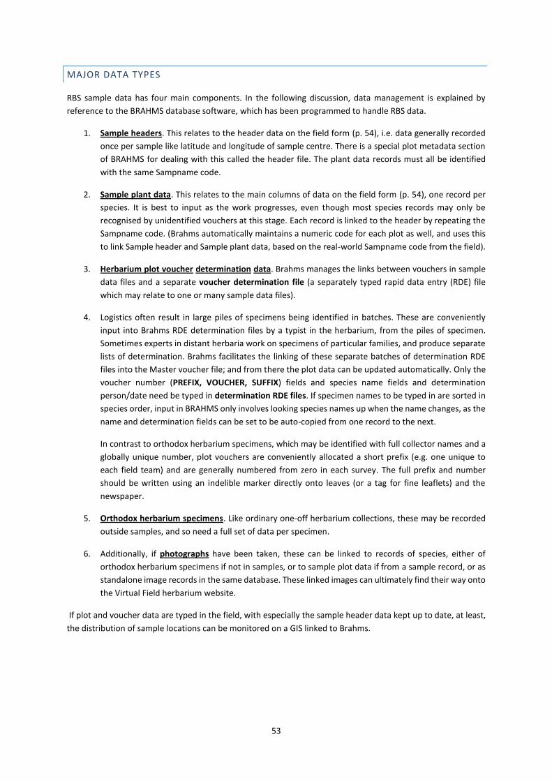
53
MAJOR DATA TYPES
RBS sample data has four main components. In the following discussion, data management is explained by
reference to the BRAHMS database software, which has been programmed to handle RBS data.
1. Sample headers. This relates to the header data on the field form (p. 54), i.e. data generally recorded
once per sample like latitude and longitude of sample centre. There is a special plot metadata section
of BRAHMS for dealing with this called the header file. The plant data records must all be identified
with the same Sampname code.
2. Sample plant data. This relates to the main columns of data on the field form (p. 54), one record per
species. It is best to input as the work progresses, even though most species records may only be
recognised by unidentified vouchers at this stage. Each record is linked to the header by repeating the
Sampname code. (Brahms automatically maintains a numeric code for each plot as well, and uses this
to link Sample header and Sample plant data, based on the real-world Sampname code from the field).
3. Herbarium plot voucher determination data. Brahms manages the links between vouchers in sample
data files and a separate voucher determination file (a separately typed rapid data entry (RDE) file
which may relate to one or many sample data files).
4. Logistics often result in large piles of specimens being identified in batches. These are conveniently
input into Brahms RDE determination files by a typist in the herbarium, from the piles of specimen.
Sometimes experts in distant herbaria work on specimens of particular families, and produce separate
lists of determination. Brahms facilitates the linking of these separate batches of determination RDE
files into the Master voucher file; and from there the plot data can be updated automatically. Only the
voucher number (PREFIX, VOUCHER, SUFFIX) fields and species name fields and determination
person/date need be typed in determination RDE files. If specimen names to be typed in are sorted in
species order, input in BRAHMS only involves looking species names up when the name changes, as the
name and determination fields can be set to be auto-copied from one record to the next.
In contrast to orthodox herbarium specimens, which may be identified with full collector names and a
globally unique number, plot vouchers are conveniently allocated a short prefix (e.g. one unique to
each field team) and are generally numbered from zero in each survey. The full prefix and number
should be written using an indelible marker directly onto leaves (or a tag for fine leaflets) and the
newspaper.
5. Orthodox herbarium specimens. Like ordinary one-off herbarium collections, these may be recorded
outside samples, and so need a full set of data per specimen.
6. Additionally, if photographs have been taken, these can be linked to records of species, either of
orthodox herbarium specimens if not in samples, or to sample plot data if from a sample record, or as
standalone image records in the same database. These linked images can ultimately find their way onto
the Virtual Field herbarium website.
If plot and voucher data are typed in the field, with especially the sample header data kept up to date, at least,
the distribution of sample locations can be monitored on a GIS linked to Brahms.
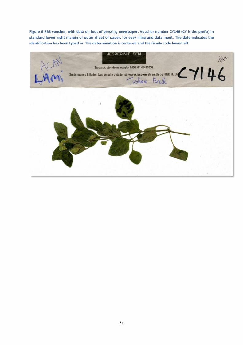
54
Figure 6 RBS voucher, with data on foot of pressing newspaper. Voucher number CY146 (CY is the prefix) in
standard lower right margin of outer sheet of paper, for easy filing and data input. The date indicates the
identification has been typed in. The determination is centered and the family code lower left.
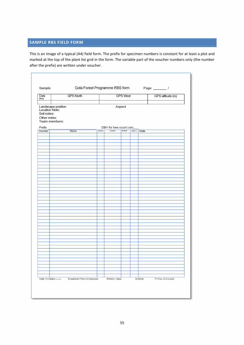
55
SAMPLE RBS FIELD FORM
This is an image of a typical (A4) field form. The prefix for specimen numbers is constant for at least a plot and
marked at the top of the plant list grid in the form. The variable part of the voucher numbers only (the number
after the prefix) are written under voucher.
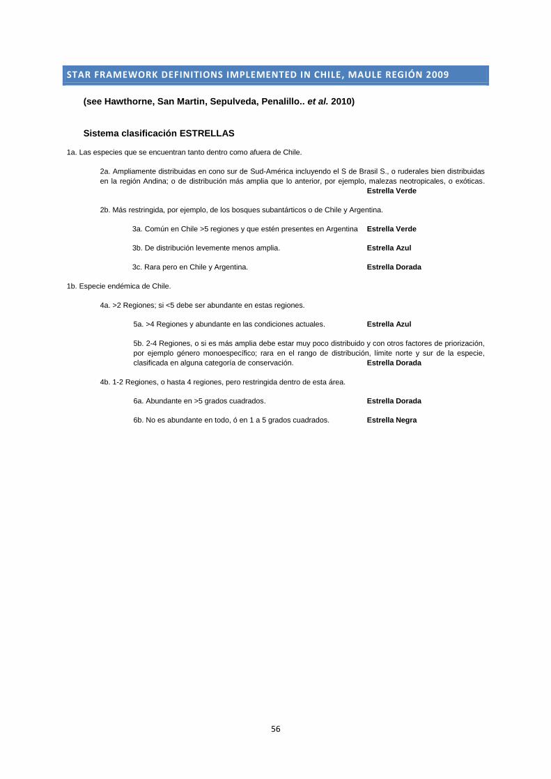
56
STAR FRAMEWORK DEFINITIONS IMPLEMENTED IN CHILE, MAULE REGIÓN 2009
(see Hawthorne, San Martin, Sepulveda, Penalillo.. et al. 2010) Sistema clasificación ESTRELLAS
1a. Las especies que se encuentran tanto dentro como afuera de Chile.
2a. Ampliamente distribuidas en cono sur de Sud-América incluyendo el S de Brasil S., o ruderales bien distribuidas
en la región Andina; o de distribución más amplia que lo anterior, por ejemplo, malezas neotropicales, o exóticas.
Estrella Verde
2b. Más restringida, por ejemplo, de los bosques subantárticos o de Chile y Argentina.
3a. Común en Chile >5 regiones y que estén presentes en Argentina Estrella Verde
3b. De distribución levemente menos amplia. Estrella Azul
3c. Rara pero en Chile y Argentina. Estrella Dorada
1b. Especie endémica de Chile.
4a. >2 Regiones; si <5 debe ser abundante en estas regiones.
5a. >4 Regiones y abundante en las condiciones actuales. Estrella Azul
5b. 2-4 Regiones, o si es más amplia debe estar muy poco distribuido y con otros factores de priorización,
por ejemplo género monoespecífico; rara en el rango de distribución, límite norte y sur de la especie,
clasificada en alguna categoría de conservación. Estrella Dorada
4b. 1-2 Regiones, o hasta 4 regiones, pero restringida dentro de esta área.
6a. Abundante en >5 grados cuadrados. Estrella Dorada
6b. No es abundante en todo, ó en 1 a 5 grados cuadrados. Estrella Negra