Rapid Prototyping and Optimization based on

Conceptual Specification for Fuzzy Applications�

Chantana Chantrapornchai Michael Sheliga Sissades Tongsima

Edwin H.-M. Sha

Research report: TR-98-4

Dept. of Computer Science and Engineering

University of Notre Dame

Notre Dame, IN 46556

Abstract

In this paper, a new framework for rapid system design and implementation for fuzzy

systems is proposed. The given system specification is separated into two components: acon-

ceptual specificationand aparameter specification. The conceptual specification defines the

system core, which is rarely changed during the system adjustment and may be implemented

in hardware at an early stage of the design process. The parameter specification defines pa-

rameters that are often changed and are implemented in software for easy adjustment. Such

a partitioning approach integrates both hardware and software capability. Two models, aBe-

havioral Network, which describes the overall system behavior, and aConceptual State Graph,

which represents the conceptual specification, are discussed. The presented methodology gives

a rapid prototyping and efficient system tuning process which, therefore, can reduce the devel-

opment cycle time and increase flexibility when designing fuzzy systems.

�This work was supported by NSF grant MIP 95-01006 and Royal Thai Government Scholarship.

1

1 Introduction

In the design of application specific systems, the iterative process of detailing specifications, de-

signing a possible solution, and testing and verifying the solution is repeatedly performed until

the solution meets user requirements (see Figure 1). However, such a repeated cycle prolongs the

system development time. The system life cycle is likely to be short due to rapid pace of im-

provements in current technology. The need for early prototyping, therefore, becomes critical to

implement a system specification and provide customers with feedback during the design process.

Significant research has been conducted on rapid system prototyping for several applications

such as digital signal processing (DSP) [9,13,19] and processor design [1,6]. The design method-

ology based on architectural synthesis was presented by Kission et. al. [10]. Their method focused

on the two main concepts: hierarchy, where a complex design is decomposed into modules and

regularity, which is aimed at design reuse. Wang and Marty presented the mechanical design

methodology [25]. Their approach explores the formalism, modeling of design problem and de-

termining a satisfactory design solution. Both approaches, however, consider design abstractions

where hardware as well as software components are hidden.

Embedding all system design components into hardware is not a good approach due to lack

of flexibility during reconfiguration. In fuzzy systems, by partitioning the system components

properly, an early prototype can be established. Our paper gives a rapid prototyping methodology

which integrates hardware and software capability and provides flexibility in exploring several

design solutions. Given a set of user requirements, a system specification which describes what

system functions are needed to satisfy the requirements is developed. Such a specification can be

abstractly divided into two parts: aconceptual specificationand aparameter specification. The

conceptual specification contains a specification core that is rarely changed during various system

adjustment while the parameter specification includes specific details which can be easily modified

during the design phase.

Figure 2 summarizes the overall prototyping methodology. First, a set of user specifications

which describe what the system does is analyzed. After that, a global high-level system speci-

fication is derived and then transformed to abehavioral network(BN). Note that the behavioral

network represents a global view of system functional behaviors. A global optimization process

2

Modification

Solution

Functional

Detail

ManufactureFinal Version

Prototype

Design Iteration Cycle

User RequirementAnalysis

Possible DesignSpecification Testing

Figure 1: System design and implementation flow

may be applied to the behavioral network to minimize the specification. Next, this behavioral net-

work is partitioned into conceptual and parameterized components. A model called aconceptual

state graph(CSG) is used to represent the conceptual specification. This model exhibits system

functions without implementation details, e.g., timing constraints or gate delays. Such a graph can

simply be mapped into an implementation model such as a finite state machine (FSM). Because

the conceptual specification will not be changed throughout the testing process, it may be quickly

implemented in hardware so as to establish a partial hardware prototype. Since finite state machine

modeling is well-developed, we use it to simplify hardware conversion and minimization [12]. Pa-

rameter specification, on the other hand, is handled by software since it describes specific details of

how the system is implemented. These details will likely change during the design iteration cycle,

and need to be easily modifiable. After several iterations of the design process, the parameters

that produce the best output with respect to the user requirements are chosen. Finally, the com-

plete prototype is achieved by implementing selected parameters, in hardware or software, and

incorporating them in the existing conceptual specification prototype.

Optimization andPartitioning

H/W Model andOptimization

SpecificationParameter Testing

Prototype

FinalVersionManufacture

AnalysisUser Requirement

HardwarePrototype

Conceptual Specification

Possible Design Solution

Design Iteration Cycle

S/W Development and Optimization

Modification

High-levelSpecification/BN

Figure 2: Proposed prototyping process

3

1.1 Fuzzy system design

Recently, fuzzy systems have been popularly used in many industrial products [14,27]. Since such

systems are designed to mimic human knowledge, the performance of the systems is as good as

knowledge given by experts. Therefore, a large number of real-time experiments are required in

order to verify the system performance. Considerable work has been done on developing hardware

implementations for general purposed fuzzy control systems. In [5, 15, 20, 23], special hardware

chips have been invented to speedup the fuzzy inference engine. Other work has concentrated

on design and implementation of fuzzy architectures and processors [2, 4, 8, 18, 24, 26]. Software

fuzzy systems are flexible but fail to provide high-speed result [17]. Although general-purposed

fuzzy hardware can yield high-speed output, prototyping such hardware is complex [8, 23]. Un-

like the others, by utilizing both hardware and software components, our approach provides rapid

prototyping for application specific fuzzy systems as well as efficient implementation.

Select Membership

Functions

Select Defuzzification

Method

Testing

Optimization and Partitioning

BN modeling

Rule Specification(CSG)

FSM Implementation

Optimizationand

S/W Implementation

Conceptual

specificationParameter

Specification

User Requirement

Analysis

Figure 3: Fuzzy system design flow

Since one of the goals of using fuzzy logic is to reduce computational complexity of designing

systems, e.g., fuzzy control systems, fuzzy logic rule bases consist of human knowledge expressed

in rule format. Figure 3 shows the proposed design approach mapped to the existing fuzzy sys-

tem design flow. First a user specifies his/her requirements, e.g., the system input/output and

system operations. After a system function is specified, membership functions and a defuzzifi-

cation method are chosen. Based on our methodology, the system specification is characterized

into two subcomponents. Since the rule base is rarely changed throughout the design process, our

4

methodology regards it as a part of the hardware prototype of the conceptual specification. The

adjustable components of the design are the membership functions and the defuzzification method.

These components become part of the software implementation of the parameter specification. In

general, the proposed approach has the following benefits:

1. rapid specification: the conceptual specification gives designers the ability to specify the

overall concept of the system which is independent of parameter setting details.

2. flexible tuning: the parameter specification and new system model allow designers to easily

adjust the parameters and consider several possible solutions in order to meet user require-

ments.

3. hardware/software capability: the integration of hardware prototype and flexible parame-

terized software naturally takes advantages of the ideas of hardware/software co-design.

4. shorter development process: partitioning the system specification into two components

allows the possibility of developing hardware and software in parallel and early prototyping.

The detail of our method will be discussed in the remainder of this paper. Section 2 presents

our system models. The prototyping methodology and co-simulation framework are discussed

in Section 3. Section 4 presents an example of prototyping a fuzzy control system. Issues of

optimization and some example are presented in Section 5. Finally, Section 6 draws conclusion

from this work.

2 System Models

A rule-based system consists of a collection of conditional statements such as IF-THEN rules. The

variables in the if-part are calledinput variableswhile the variables in the then-part are called

output variables. A particular value of an input/output variable is called aninput/output instance.

In a fuzzy system, the value of these variables specified in the rules can belinguistic variables.

Such systems can be modeled by aBehavioral Network:

5

Definition 2.1 A Behavioral Network (BN) is a labeled directed acyclic graph (DAG)G = (V;E; l)

whereV is a set of vertices,vi 2 V; 1 � i � n, representing rules, input domains and output do-

mains,E � V � V is a set of dependence edges,ej 2 E; 1 � j � m, denoted byu e�! v for

u; v 2 V , andl is a set of edge labels(x; z) for ue�!v 2 E wherex is an input variable ofv andz

is the value ofx.

h

hhg g

g-Z

ZZ~

XXXz

���*

���1XXXz���1

B(x,M)

C

A(x,L)

Ix

Iy

(z,H)

(z,H)

(z,L)

Oz

(x,H)(y,H)

(a) BN

?��

i i i

i- -XXXXXXXXz

s0 s1

(x, H)/(z,H)

s3(y,H)/(z,H)(x,M)/�

(x,L)/(z,L)

s2

(b) CSG

Figure 4: System models

Figure 4(a) models the following rules:

IF x = L THEN z = L

IF x = M andy = H THEN z = H

IF x = H THEN z = H

wherex; y andz are input/output variables. The values ofx; y andz can beL;M;H which stand

for low, mediumandhigh linguistic variables.Ix; Iy andOz are input/output domains which, in this

case, aretemperature, humidityandfan speeduniverses respectively. NodesA;B andC represent

each rule. An edge label represents a firing condition for each node. A pathIx; A;Oz, denoted by

Ixp Oy , with labels(x; L); (y; L) corresponds to the first rule while a set of pathsIx; B;Oz and

Iy; B;Oz correspond to the second rule and so on.

The behavioral network presents a global view of system behavior while theConceptual State

Graphpresents state-oriented behaviors of the rules.

Definition 2.2 A Conceptual State Graph (CSG)G = (S; I;O;E; !) is a connected directed edge-

weighted graph whereS is a set of nodessi 2 S; 1 � i � p, representing states of the graph,I

is the set of inputs,O is the set of outputs including�, E � S � S is a set of edges, denoted by

sie�!sj or esi;sj , si 2 S; sj 2 S, and! is a function fromE to I� O, representing the set of edge

weights, denoted byx=y, wherex 2 I andy 2 O.

6

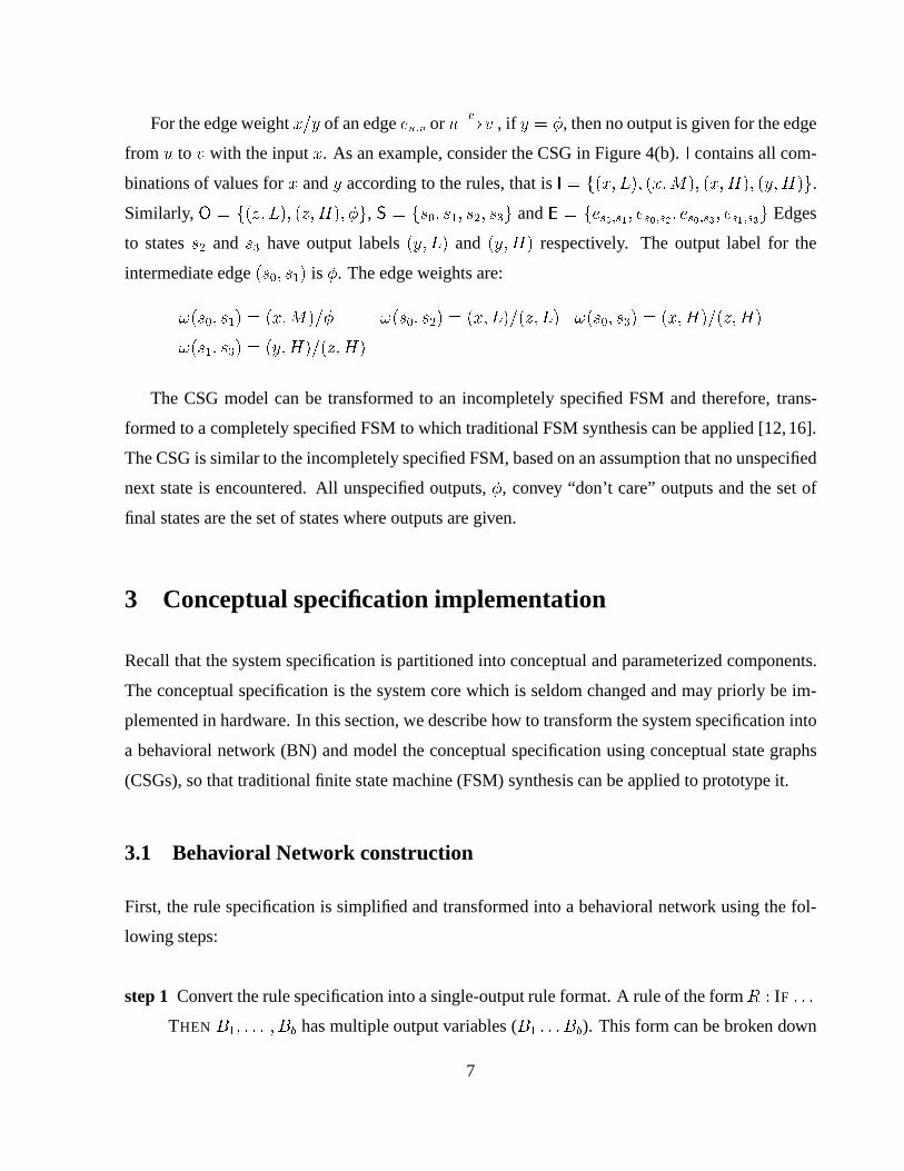
For the edge weightx=y of an edgeeu;v orue�!v , if y = �, then no output is given for the edge

from u to v with the inputx. As an example, consider the CSG in Figure 4(b).I contains all com-

binations of values forx andy according to the rules, that isI = f(x; L); (x;M); (x;H); (y;H)g.

Similarly,O = f(z; L); (z;H); �g, S = fs0; s1; s2; s3g andE = fes0;s1; es0;s2; es0;s3; es1;s3g Edges

to statess2 and s3 have output labels(y; L) and (y;H) respectively. The output label for the

intermediate edge(s0; s1) is �. The edge weights are:

!(s0; s1) = (x;M)=� !(s0; s2) = (x; L)=(z; L) !(s0; s3) = (x;H)=(z;H)

!(s1; s3) = (y;H)=(z;H)

The CSG model can be transformed to an incompletely specified FSM and therefore, trans-

formed to a completely specified FSM to which traditional FSM synthesis can be applied [12,16].

The CSG is similar to the incompletely specified FSM, based on an assumption that no unspecified

next state is encountered. All unspecified outputs,�, convey “don’t care” outputs and the set of

final states are the set of states where outputs are given.

3 Conceptual specification implementation

Recall that the system specification is partitioned into conceptual and parameterized components.

The conceptual specification is the system core which is seldom changed and may priorly be im-

plemented in hardware. In this section, we describe how to transform the system specification into

a behavioral network (BN) and model the conceptual specification using conceptual state graphs

(CSGs), so that traditional finite state machine (FSM) synthesis can be applied to prototype it.

3.1 Behavioral Network construction

First, the rule specification is simplified and transformed into a behavioral network using the fol-

lowing steps:

step 1 Convert the rule specification into a single-output rule format. A rule of the formR : IF : : :

THEN B1; : : : ; Bb has multiple output variables (B1 : : : Bb). This form can be broken down

7

into a group of rules, each of which has a single output variable, e.g.,R1: IF : : : THEN B1,

: : : , Rb: IF : : : THEN Bb

step 2 Convert the rule into aconjunctive form, e.g., IF X1 and X2 and : : : and Xm THEN Y .

The disjunctive clausesA andB in the form: IF A or B THEN C is broken down into

two disjunctive rules:R1 : IF A THEN C; andR2 IF B THEN C. Further details of this

conversion can be found in [7].

step 3 Construct a behavioral network according to Definition 2.1. The set of verticesV is fRi :

1 � i � ng[fIj : 8Ij 2 Ig[fOk : 8Ok 2 Og, wheren is the total number of single-output

rules,I is the set of all input domains, andO is the set of all output domains. The set of

edgesE is constructed as follows:Rie�! Rh 2 E if an output ofRi is required byRh.

Further,Ije�!Ri 2 E, if Ri requires an input from domainIj. Similarly,Ri

e�!Ok 2 E, if

Ri produces an output in domainOk. Edge labels are defined for edgeue�!v 2 E as a tuple

(x; z) wherex is v’s input variable andz is v’s value.

step 4 Restructure the BN by applying the topological sort. The BN is ordered by levels (also

called stages). The topological order can be briefly described as follows: if vertexi produces

an output which is required by vertexj (i! j), i has to be in levelk andj in level l, where

k < l. Furthermore, the vertices which yield values for the same output domain in the BN

are placed in the same level in the sorted BN. Note that in each level, there may be several

vertices producing outputs to different domains.

step 5 Apply a high level optimization to the BN. An optimization process is applied on the fly

to minimize the global specification and reduce the computation time. Since the number of

vertices in the BN determines the total computation time for each inference execution, min-

imizing a number of vertices in the BN is equivalent to optimizing the global specification.

In this paper, the optimization process [3] for our design example is illustrated in Section 5.

step 6 Group vertices in the BN. The grouping process can be described as follows: for rule

vertices with the same topological order, consider their outgoing labels(x; z). All vertices

which have the same output variablex are assigned to the same CSG. Note that the notation

Gr(x; j) conveys a group of vertices at levelj with input variablex.

8

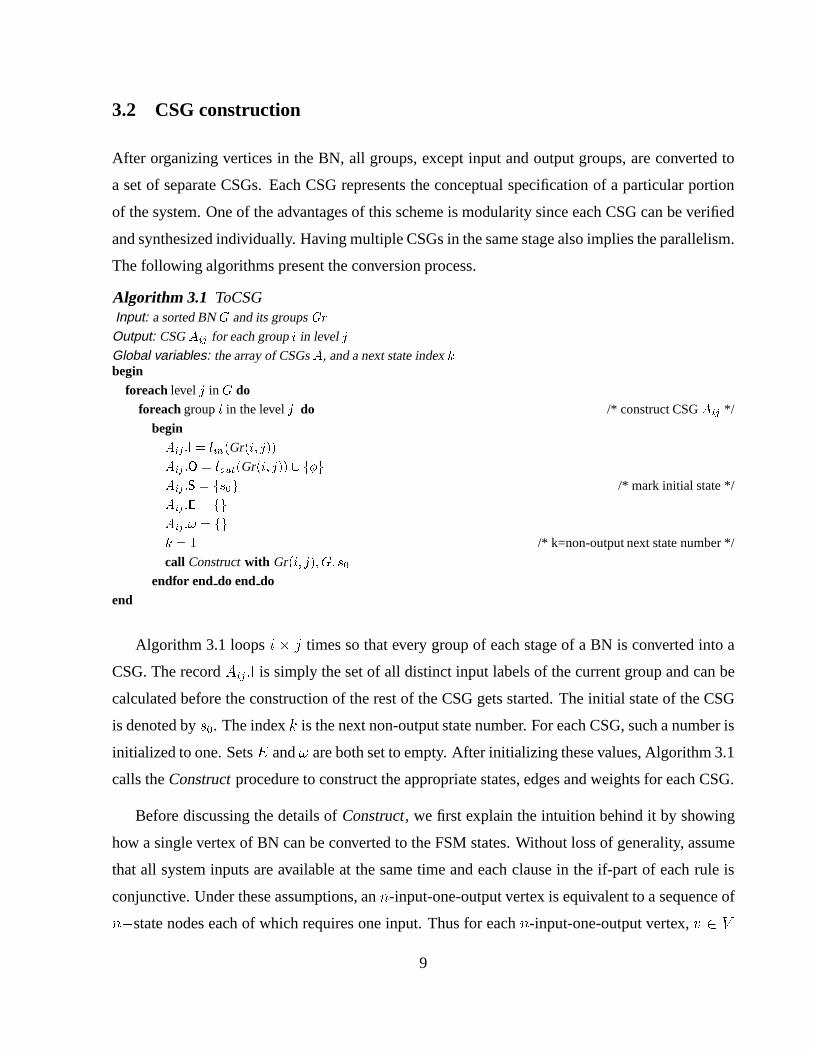
3.2 CSG construction

After organizing vertices in the BN, all groups, except input and output groups, are converted to

a set of separate CSGs. Each CSG represents the conceptual specification of a particular portion

of the system. One of the advantages of this scheme is modularity since each CSG can be verified

and synthesized individually. Having multiple CSGs in the same stage also implies the parallelism.

The following algorithms present the conversion process.

Algorithm 3.1 ToCSGInput: a sorted BNG and its groupsGr

Output: CSGAij for each groupi in level j

Global variables: the array of CSGsA, and a next state indexkbegin

foreach level j in G doforeachgroupi in the levelj do /* construct CSGAij */

beginAij :I = lin (Gr(i; j))

Aij :O = lout (Gr(i; j)) [ f�g

Aij :S = fs0g /* mark initial state */

Aij :E = fg

Aij :! = fg

k = 1 /* k=non-output next state number */

call Constructwith Gr(i; j); G; s0endfor end do end do

end

Algorithm 3.1 loopsi � j times so that every group of each stage of a BN is converted into a

CSG. The recordAij:I is simply the set of all distinct input labels of the current group and can be

calculated before the construction of the rest of the CSG gets started. The initial state of the CSG

is denoted bys0. The indexk is the next non-output state number. For each CSG, such a number is

initialized to one. SetsE and! are both set to empty. After initializing these values, Algorithm 3.1

calls theConstructprocedure to construct the appropriate states, edges and weights for each CSG.

Before discussing the details ofConstruct, we first explain the intuition behind it by showing

how a single vertex of BN can be converted to the FSM states. Without loss of generality, assume

that all system inputs are available at the same time and each clause in the if-part of each rule is

conjunctive. Under these assumptions, ann-input-one-output vertex is equivalent to a sequence of

n�state nodes each of which requires one input. Thus for eachn-input-one-output vertex,v 2 V

9

of the BN, a collection of state nodes that form ann-edge path, with input labels corresponding to

the input labels ofv, can be constructed.

Figure 5(a) presents vertexA with n incoming edges and only one output edge. Figure 5(b)

shows a path, denoted bys0p sn , consisting of state nodesfs0; s1 : : : sng in the new CSG. The

initial state is represented by nodes0. Nodes1 represents the state after receiving input(I; 1) and

so on. Finally, nodesn denotes the state that detects the last input(I; n) and emits the output

(O; 1).

g -?-

6

.......... A(I2; 1)

(I1; 1)

(In; 1)

(O; 1)

(a) a node in

a BN

i i i i- -s1 s2 sn

(I2; 1)=�

s0

(In; 1)=(O; 1)(I1; 1)=�

(b) correspond-

ing state nodes

in a CSG

Figure 5: BN to CSG

If a BN consists ofm nodes and each of which hasn distinct input and output labels, the

total number of edges in the corresponding CSG is equal tom � n. Normally, any two nodes in

a BN may require the same, non-distinct, input edge label. Therefore, allowing them to share a

single edge reduces the total number of edges in the CSG. The minimized CSG will simplify the

conversion of the graph to the corresponding FSM hardware. As long as all input labels of a vertex

v in the BN are specified as an edge of the appropriate path in the CSG, the input labels can be

arranged in any order. Also, the input labels of the BN have to be selected carefully if the total

number of edges in CSG are to be minimized. Algorithm 3.2 presents a greedy heuristic for this

problem.

Algorithm 3.2 ConstructInput: a set of verticesN � V , a sorted BNG, a current starting statescOutput: an update the current state graphAij

beginl max= Extract-Max-Input-Label(N;G) /* find the input edge label with max occurrences */

if l 6= (NULL)

then begin/* partition vertices into two groupsP andQ */

10

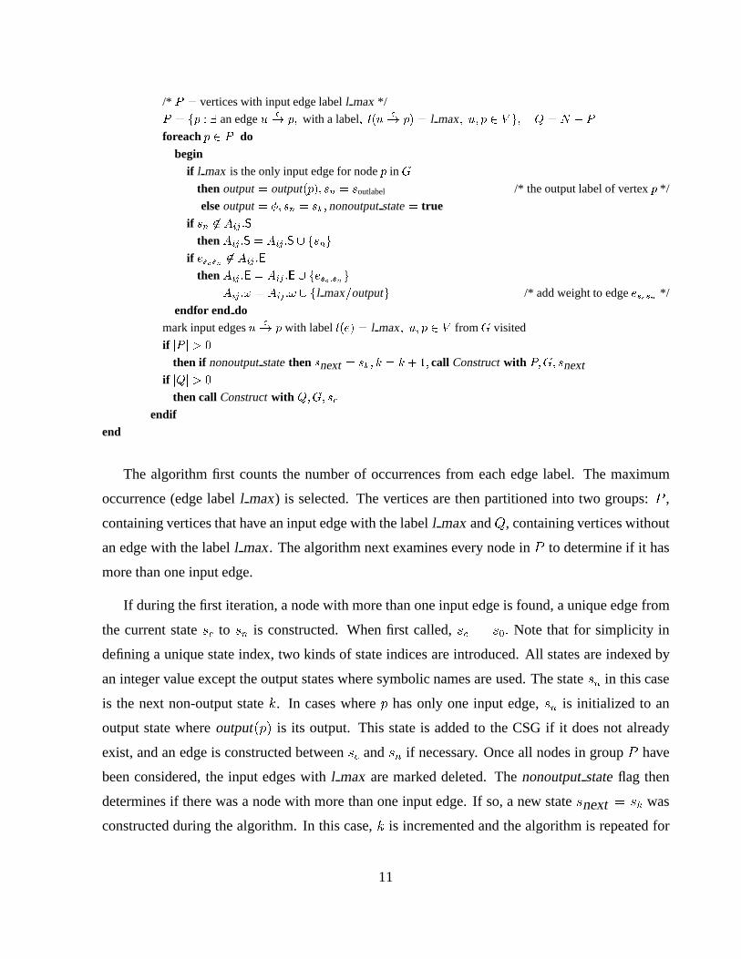
/* P = vertices with input edge labell max */

P = fp : 9 an edgeue�! p; with a label; l(u

e�! p) = l max; u; p 2 V g; Q = N � P

foreachp 2 P dobegin

if l max is the only input edge for nodep in G

then output= output(p); sn = soutlabel /* the output label of vertexp */

elseoutput= �; sn = sk; nonoutputstate= trueif sn 62 Aij :S

thenAij :S = Aij :S [ fsng

if escsn 62 Aij :E

thenAij :E = Aij :E [ fesc;sng

Aij :! = Aij :! [ fl max=outputg /* add weight to edgeescsn */

endfor end domark input edgesu

e�! p with labell(e) = l max; u; p 2 V fromG visited

if jP j > 0

then if nonoutputstatethen snext = sk; k = k + 1; call Constructwith P;G; snextif jQj > 0

then call Constructwith Q;G; sc

endifend

The algorithm first counts the number of occurrences from each edge label. The maximum

occurrence (edge labell max) is selected. The vertices are then partitioned into two groups:P ,

containing vertices that have an input edge with the labell maxandQ, containing vertices without

an edge with the labell max. The algorithm next examines every node inP to determine if it has

more than one input edge.

If during the first iteration, a node with more than one input edge is found, a unique edge from

the current statesc to sn is constructed. When first called,sc = s0: Note that for simplicity in

defining a unique state index, two kinds of state indices are introduced. All states are indexed by

an integer value except the output states where symbolic names are used. The statesn in this case

is the next non-output statek. In cases wherep has only one input edge,sn is initialized to an

output state whereoutput(p) is its output. This state is added to the CSG if it does not already

exist, and an edge is constructed betweensc andsn if necessary. Once all nodes in groupP have

been considered, the input edges withl max are marked deleted. Thenonoutputstateflag then

determines if there was a node with more than one input edge. If so, a new statesnext = sk was

constructed during the algorithm. In this case,k is incremented and the algorithm is repeated for

11

P with a new initial state,snext. The algorithm is also repeated forQ using the old initial state.

These two recursions stop after all input edges of a given set of vertices are considered.

hl

lh

hl

�����: XXXXXz

�����>PPPPPq ���

��:

XXXXXz���

�:

�����3

P

C

B

A

ST

(S;H)

(S;H)

(S; L)

(P;M)

(P;H)(P;L)

(T;H)

(T;H)

(a) BN

��

jj

��

�

?

� SSw

s0

s(S;L) s(S;H)

(P;H)=(S;H)

(T;H)=�

(P;L)=(S; L)

(P;M)=(S;H)

s1

(b) Corresponding

CSG

Figure 6: Applying theConstructAlgorithm

Consider the example BN in Figure 6(a) and verticesA;B,andC. The algorithm first selects

label (T;H) since there are two vertices requiring such an input label. Thus,P = fA;Bg while

Q = fCg. In Figure 6(b), an edges0e�! s1 is constructed with weights(T;H)=�. Since the

initial state of the CSG iss0, the transition froms0 to s1 is constructed and shared by vertices

A andB in the BN. The edges with input label(T;H) of both verticesA andB are eliminated

from the BN and the next non-output statek is incremented. Now the current initial state ofA

andB is s1, conveying that at states1 input (T;H) has been detected. The algorithm recursively

constructs transitions froms1 for the verticesA andB which will distinguish between them. The

paths0p s(S;H) with labels(T;H)=� and(P;H)=(S;H) corresponds to the vertexB in the BN

while the paths0p s(S;L) with labels(T;H)=� and(P; L)=(S; L) corresponds to the vertexA.

For the vertexC, because there is the only one input and the output state(S;H) is already defined,

only the edges0e�!s(S=H) is constructed. From this CSG, the transitions to statess(S;L) ands(S;H)

emit outputs. After obtaining the CSG, the hardware prototype can be developed using a traditional

finite state machine synthesis. Traditional FSM optimizations may be applied to minimize the FSM

before the hardware is implemented.

12

4 Design Example

Since one of the goals of using fuzzy systems is to reduce computational complexity while design-

ing systems, fuzzy systems consist of human knowledge described in the rule format. In order to

compute system outputs, the given input instance is transformed (orfuzzified) into input linguistic

variables usingmembership functions. Then fuzzy inference process computes possible conse-

quences. The fired output linguistic variables are collected anddefuzzifiedinto a particular output

instance.

According to the fuzzy inference engine, fuzzy design components can be briefly described as

follows. First, a user specifies his requirements, e.g., the system input/output and system opera-

tions. After a system function is specified, designers choose membership functions and a defuzzi-

fication method. The system is then implemented and its performance is evaluated.

4.1 The behavioral network and conceptual specification

We now consider designing a temperature control system for the oven found in [21]. The control

system has two temperature input variablesx1 andx2 and outputs a new temperatureu to which

the oven temperature should be adjusted. The following is the set of rules.

1. IF x1 = low (x1; L) and x2 = low (x2; L) THEN u = high (u;H)

2. IF x1 = low (x1; L) and x2 = medium(x2;M) THEN u = medium(u;M)

3. IF x1 = low (x1; L) and x2 = high (x2; H) THEN u = low (u; L)

4. IF x1 = medium(x1;M) and x2 = low (x2; L) THEN u = high (u;H)

5. IF x1 = medium(x1;M) and x2 = high (x2; H) THEN u = low (u; L)

6. IF x1 = high (x1; H) and x2 = low (x2; L) THEN u = high (u;H)

7. IF x1 = high (x1; H) and x2 = medium(x2;M) THEN u = medium(u;M)

8. IF x1 = high (x1; H) and x2 = high (x2; H) THEN u = low (u; L)

The tuple next to each clause is a shorthand notation of the clause’s linguistic variable. Fig-

ure 7(a) presents the BN for this one-stage set of rules where the system inputs are temperatures

x1 andx2 and the temperature output isu. Vertices 1–8 correspond to rules 1–8. An edge label is

13

a tuple(x; z) wherex is either variablex1, x2, or u andz is a linguistic variables with respect to

domain(x1), domain(x2), or domain(u) respectively.

2 3 41 5 6 7 8

uO

(x2,M)

(u,M)

(x2,H)

(x2,L)

(x2,H)

(x2,L)

(x2,L)(x2,M)

(x2,H)

(x1,L)

(x1,M)(x1,H)

(u,H) (u,L) (u,H) (u,L) (u,H) (u,M) (u,L)

I_x2I_x1

(a) Behavioral Network

s1

s0

(x2,M)/(u,M)

(x2,M)/(u,M)

(x2,L)/(u,H)s_(u,H)

s_(u,M)

s_(u,L)s2

s3

(x2,H)/(u,L)

(x2,H)/(u,L)

(x2,

L)/(u

,H)(x2,

L)/(u,

H)

(x2,H)/(u,L)

(x1,L)/

(x1,M)/

(x1,H)/ φ

φ

φ

(b) CSG

Figure 7: Behavioral network and CSG

In this example, the BN contains linguistic variables, associated with membership functions,

which are parts of the parameter specification. Figure 7(b) shows the CSG obtained from Algo-

rithm 3.1 for the BN in Figure 7(a).S is fs0; s1; s2; s3; s(u;M); s(u;L); s(u;H)g. The transitions to

statess(u;M); s(u;L), ands(u;H) output temperature valuesmedium, low, andhigh respectively. Fig-

ure 8 shows some VHDL simulation result for the CSG in Figure 7(b). The reset signal is activated

after each output is given. Statess(u;H); s(u;M) ands(u;L) are encoded to statess4; s5 ands6 re-

spectively. Linguistic variables(x1; L); (x1;M); (x1; H); (x2; L); (x2;M); (x2; H) are represented

by 000; 001; 010; 011; 100 and101 while output variables(u; L); (u;M); (u;H); � are encoded as

00; 01; 10 and11 respectively.

4.2 Parameter specification

Since all input and output variables are temperatures, the same membership functions for all vari-

ables are used. Figure 9(a) defines these functions. The temperature domain is restricted to be-

tween 0 and 500 degrees centigrade. Because of the nature of fuzzy rules, an input instance may

fire more than one rule, depending on the given membership functions. A mapping relation�u

is defined for each instance fromU to 2jV j whereU is an input instance domain andV is a set

of linguistic variables in domainU . Given an input instancei, �u(i) returns the corresponding

14

/nxt_state

/clk

/x(2)(1)(0)/rst/z

(1)(0)

state s0s1

000 011

s1

s4s0

s3

s3

s6

s0

s2

s2

s5

11 00 11 10 11 01

001 101 010 100

Figure 8: Simulation results of circuits implementing Figure 7(b)

linguistic variable(s). Based on the membership functions defined in Figure 9(a),�xi relations

are defined for each of the temperature instances. In this example, according to Figure 9(a),

�x1(t) 2 ffHg; fLg; fMg; fL;Mg; fM;Hgg, for input x1 as well asx2. For input instance,

for x1 = 125, �x1(125) = fL;Mg. We use the weighted average method to defuzzify the output

values(z� =P

�(z)zP�(z)

) [21].

4.3 Simulation framework

According to the fuzzy inference process, a special calculation is required to determine the output

strength of each rule given the associated input strengths. Let�Xij(xj) denote a membership

function corresponding to the linguistic variableXij and the current input instancexj for rule i.

Let�Yi(y) be a membership function corresponding to the linguistic variableYi and output instance

y for rule i. Suppose a rule requiresm inputs. Given input instancex1; : : : ; xm, for each rulei,

Equation 1 determines a modified output function�0Yi(y) that is used in the defuzzification process

�0Yi(y) =

8<:

�Yi(y) if �Yi(y) < r

r otherwise(1)

where the strengthr, calculated by Equation 2, is the limit of the output strengthYi.

r = minmj=1�Xij

(xj) (2)

15

If more than one rules give the same outputYi and therefore generates a new function�0Yi(y), each

�0Yi(y) is combined by using themax operation.

�00Yi(y) = max(�0

Yi(y)) (3)

Based on the above equations and the given CSG, the following algorithm presents the infer-

ence process.

Algorithm 4.1 TraverseCSGInput: a CSGA, conclusion functionF , input instances I

Output: an output valueo

beginB[(u; i)] = 0:0;8 linguistic variablei

foreach input sequenceft1 : : : tng � I according toA dor =1;S = f(s0; r; 1)g /* initial states0 2 A :S */

while S is not emptydo begin(cur state; r; i) = pop(S); oldr = r

foreach l 2 �xi(ti) do beginr = oldr ; r = min(r; �(xi;l)(ti))

s = StateOf(xi; l) from cur state

if s 6= nullthen if an edge fromcur stateto l gives outputu

thenB[u] = max(B[u]; r)

elsex = (s; r; i+ 1)

push(S; x)

end doendforend doendwhile

end doendforo = F(B)

end

Let B be the output buffer and each elementB[p] contains a current cut value (strength) for

functionp. For instance,B[(u; i)] keeps the current strength that output linguistic variableu is i.

StackS contains the current minimum valuer computed by Equation 2. FunctionStateOfreturns

the next state according to the given input variable(xi; l), wherel is a linguistic variable in�xi(ti)

and functionF defines the defuzzification procedure.

Now let us briefly trace the algorithm. In this example, two input instances,t1 and t2, are

required. Lett1 be 80 andt2 be 85. Let�(x1;L)(t1) = 0:93, �(x1;M)(t1) = 0:1, �(x2;L)(t2) = 0:89

16

and�(x2;M)(t2) = 0:07. Starting from the initial states0, �x1(80) = fL;Mg. For (x1; L), the

next state iss1; r = 0:93 while i + 1 = 2. Hence, the tuple(s1; 0:93; 2) is pushed ontoS.

Similarly, for (x1;M), the tuple(s3; 0:1; 2) is saved toS. During the next iteration,pop(S) sets

cur state= s3; r = 0:1; i = 2 where�x2(t2) = �x2(85) = fL;Mg. The transition froms3 with

the input(x2; L) gives an output(u;H). Nowr = min(r; �(x2;L)(85)) = min(0:1; 0:89) = 0:1 and,

therefore,B[(u;H)] = 0:1. Next, the algorithm pops(cur state= s1; r = 0:93; i = 2). For t2 =

85, �x2(85) = fL;Mg. From states1 with (x2; L) as the input, the transition gives output(u;H)

with strengthr = min(0:93; 0:89) = 0:89 and the overallB[(u;H)] = max(B[(u;H)]; 0:89) =

max(0:1; 0:89) = 0:89. Finally, the transition from states1 with input(x2;M) yields output(u;M)

with the strength of the output temperature being medium equal tomin(0:93; 0:07) = 0:07. The

graphical result presenting the cuts for the output membership functionsM andH is shown in

Figure 9(b).

� -���

TTT

%%%SSS

6�

1

210 350 50070

L M H

(a) Tempera-

ture func.

� -���

TTT

%%%S

SS

6............................................

............................................................

�

210 350 50070

L M H10.89

0.07

(b) A cut for

outputs

6

��............

....� -

�

210 50070

M H1

350

0.89

0.07

343

(c) Defuzzi-

fication

Figure 9: Membership functions

The area bounded by both output membership functionsmediumandhigh and their strengths

are shown in Figure 9(c). By using the weighted average method to defuzzify, the output temper-

atureu = 343 is obtained. This output may be fed back to the system and the buffer may be reset

to re-run the system. If the system does not work properly, designers can modify the membership

functions. The defuzzification method can also be reselected depending on the designers.

Figure 10 presents the integration of each of the system components. The hardware components

contain rule base transformed into the combinational circuits. The software simulator includes pa-

rameterized components such as membership functions. Here we fix our defuzzification method to

be the weighted average method. Therefore, we implement it in hardware to speedup the compu-

tation. The given input instance is first fuzzified to be a strength value of each linguistic variable.

17

t ... t1 n

Fuzzification

Defuzzification H/W

system output (o1,..,ok)

Hardware Prototype

(combinational circuit)

GeneratorInput

rule base implementation

Next state register

Stack (S),Output (B)

by TraverseCSGcompute rule strength

membership function

set/reset

next_stateInitial state

output

software simulator

output feedback

feedback calculation

initial system input

Figure 10: Simulation framework

The input generator produces the proper inputs according to the non-zero strength linguistic vari-

able and feeds them into the rule-based hardware. Meanwhile, the strength of the rule is computed

in software using given membership functions. Once the output of a fired rule is derived from the

hardware, it is converted back into the proper linguistic variable and saved to bufferB. Possible

next states are also collected and saved in the bufferS. The defuzzification function takes outputs

from the output buffer and evaluates the final output. This output may be fed back to the system to

re-run the simulation.

5 Optimization of Fuzzy Systems

For complex fuzzy systems, the system specification can be minimized before prototyping, e.g.,

overlapped membership functions can be combined. Since a rule in a fuzzy system or a vertex in

a BN can be viewed as afuzzy relation, constructed from the given membership functions [22],

combining these relations is equivalent to merging fuzzy rules. In order to reduce the execution

time during the inference computation, two fundamental set operations,union andcomposition,

are carefully applied to certain relations based on the traditional fuzzy inference process [7,11]. In

the resulting relations, the redundant calculations, due to the overlap of the membership functions,

are eliminated. Combining the relations is analogous to merging vertices in the BN. Since the

number of vertices in the BN may be related to the number of states in some CSGs, which will be

implemented in hardware, reducing them can decrease the hardware size. Further, the longest path

18

between the input and output vertices, which implies the execution time for a simulation, may also

be decreased when the number of vertices are minimized. In general, the goal of our optimization

is to carefully combine the vertices in the BN so as to reduce the inference processing time.

The dimensionalityof the relation corresponding to a vertex is defined to be the number of

distinctinput and output variables of the rule. Since the computation time and the memory usage of

a vertex during the fuzzy calculation is related to the number of variables associated with the vertex,

the dimensionality of a vertex is important. A large dimensionality of a fuzzy relation will lead to

time consuming computation during the inference process. We, therefore, restrict the increase of

the dimensionality of the vertices during the minimization process. For both operations, necessary

conditions for combining vertices are established to control the new vertex ’s dimensionality and

check the validity during the combining process.

5.1 Dimensionality-based union

To apply the union operation properly, the following is a necessary condition for the union of two

vertices in the BN.

NECESSARYUNION CONDITION:

Let Uv denote the set of all distinct input variables of the vertexv, v 2 V . For any two distinct

verticesu andv that are in the same topological order and whose output variables are identical, a

new vertexn is generated using the union operation, if and only ifUu � Uv or Uv � Uu.

Based on the above condition, the union of the vertices in the BN can be defined as:

PROCEDUREUnion:

Let G = (V;E; l) be ann-stage BN obtained from steps 1–4 of the behavioral network construc-

tion, and letVs;d denote the set of vertices in stages whose output variable isd1. For all distinct

output variablesd and0 < s < n, compareUu andUv; 8u; v 2 Vs;d; u 6= v.

1. If the Union Condition is satisfied, apply the union operation to their fuzzy relations and

1whens = 0 ands = n, Vs is the vertices representing the input domains and output domains,I andO, respec-

tively, and whens = 1, V1 refers to the vertices in the first topological level of the BN.

19

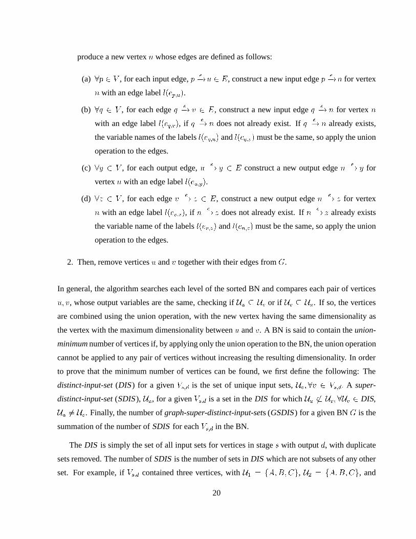
produce a new vertexn whose edges are defined as follows:

(a) 8p 2 V , for each input edge,pe�!u 2 E, construct a new input edgep

e�!n for vertex

n with an edge labell(ep;u).

(b) 8q 2 V , for each edgeqe�! v 2 E, construct a new input edgeq

e�! n for vertexn

with an edge labell(eq;v), if qe�! n does not already exist. Ifq

e�! n already exists,

the variable names of the labelsl(eq;n) andl(eq;v) must be the same, so apply the union

operation to the edges.

(c) 8y 2 V , for each output edge,ue�! y 2 E construct a new output edgen

e�! y for

vertexn with an edge labell(eu;y).

(d) 8z 2 V , for each edgeve�! z 2 E, construct a new output edgen

e�! z for vertex

n with an edge labell(ev;z), if ne�! z does not already exist. Ifn

e�! z already exists

the variable name of the labelsl(ev;z) andl(en;z) must be the same, so apply the union

operation to the edges.

2. Then, remove verticesu andv together with their edges fromG.

In general, the algorithm searches each level of the sorted BN and compares each pair of vertices

u; v, whose output variables are the same, checking ifUu � Uv or if Uv � Uu. If so, the vertices

are combined using the union operation, with the new vertex having the same dimensionality as

the vertex with the maximum dimensionality betweenu andv. A BN is said to contain theunion-

minimumnumber of vertices if, by applying only the union operation to the BN, the union operation

cannot be applied to any pair of vertices without increasing the resulting dimensionality. In order

to prove that the minimum number of vertices can be found, we first define the following: The

distinct-input-set(DIS) for a givenVs;d is the set of unique input sets,Uv; 8v 2 Vs;d: A super-

distinct-input-set(SDIS), Uu, for a givenVs;d is a set in theDIS for whichUu 6� Uv; 8Uv 2 DIS,

Uu 6= Uv. Finally, the number ofgraph-super-distinct-input-sets (GSDIS) for a given BNG is the

summation of the number ofSDIS for eachVs;d in the BN.

TheDIS is simply the set of all input sets for vertices in stages with outputd, with duplicate

sets removed. The number ofSDIS is the number of sets inDIS which are not subsets of any other

set. For example, ifVs;d contained three vertices, withU1 = fA;B;Cg, U2 = fA;B;Cg, and

20

U3 = fA;Bg, then theDIS will be ffA;B;Cg; fA;Bgg: The setfA;B;Cg is included only once

in theDIS. The number ofSDIS will be one sincefA;Bg is a subset offA;B;Cg. The following

theorem follows from theUnion procedure and the definition ofGSDIS.

Theorem 5.1 Given a sorted behavioral networkG = (V;E; l), without increasing the dimension-

ality of the resultant vertices, the union-minimum number of vertices ofG produced by theUnion

procedure is the number of graph-super-distinct-input-sets (GSDIS).

In order to prove the above property, we first prove that the union operation does not change

the number ofGSDIS in a BN.

Lemma 5.2 Given a sorted behavioral networkG = (V;E; l), without increasing the dimension-

ality of the resultant vertices, each union operation will not change the number of GSDIS.

Proof: Given a sorted behavioral networkG = (V;E; l), according to the the Union Condi-

tion, only vertices with the same output can be combined and the resulting vertex will also have the

same output as the original vertices. In general, the union operation can only take place between

vertices that are in the sameVs;d, or vertices that are the result of the union of two vertices inVs;d.

Hence, if we can prove that the above property is true for oneVs;d, it will be true for the entire BN.

Consider a particularVs;d, and two vertices inG, A andB that are combined to produce a new

vertexA [ B in G0. Without loss of generality, we consider two cases:UA � UB andUA = UB.

Under this assumption,UA[B = UB. Therefore, ifUB was aSDIS, so isUA[B, and ifUB was not a

SDIS, neither isUA[B. If UA � UB, thenUA was not aSDIS. On the contrary, ifUA = UB, then it

still is a SDIS. In both cases, after the vertices have been combined, the number ofSDIS will not

have changed. 2

We now prove Theorem 5.1.

Proof: (Theorem 5.1) Consider a BNG with n GSDIS. Let us assume that there exists a BN

G0, that can be obtained from BNG using only the union operation, for which there are onlyn� 1

GSDIS. However, sinceG0 was obtained fromG, using only the union operation, and the union

operation does not change the number ofGSDIS (Lemma 5.2), the total number ofGSDIS in the

original BN must have also beenn� 1. This contradicts our assumption thatn GSDIS existed in

21

the original BN. Therefore,G0 cannot haven� 1 vertices or less. Similarly, the above idea can be

applied to prove the case thatG0 containsn+1 or moreGSDIS. Consequently, the union-minimum

number of vertices must be equal to the number ofGSDIS. 2

By theUnion procedure and Theorem 5.1, the vertices whose input sets are notSDIS will be

eliminated during theUnion procedure.

5.2 Composition

Now we consider the composition operation. The following defines the condition for the compo-

sition of two vertices in the BN.

NECESSARYCOMPOSITION CONDITION:

Let indegree(v) denote the number of parents of vertexv andoutdegree(v) denote the number

of children of the vertexv, v 2 V . For verticesu; v such that9 an edgeue�! v 2 E, the

composition operation is applied if and only ifindegree(v) = 1, that is,u is the only parent ofv.

According to the above condition, theComposition procedure can be defined as:

PROCEDUREComposition:

LetG = (V;E; l) be the resulting BN after applying steps 1–4 of the behavioral network construc-

tion and letN be a total number of stages inG. For every vertexv in stages, from s = n�2 down

to 1, consider every edgeue�!v 2 E, andv 62 Vn:

1. If the Composition Condition is satisfied, apply the composition operation to their fuzzy

relations and produce a new vertexn

2. Assignn the same topological order asu.

3. The edges and edge labels forn are defined as following:

(a) 8p 2 V , for each input edgepe�! u 2 E, construct a new edgep

e�! n with an edge

labell(ep;u).

22

(b) 8q, for each output edgeve�! q 2 E, construct a new edgen

e�! q with an edge label

l(ev;q).

4. Then, remove vertexv together with its edges fromG.

5. If outdegree(u) = 0, remove vertexu together with its edges.

During theComposition procedure, the composition operation is applied to the two depen-

dent vertices that satisfy the Composition Condition. The BN is said to contain thecomposition-

minimumnumber of vertices if there exists no pair of vertices where the composition operation

can be applied assuming only the composition operation is used. The following theorem shows the

composition-minimum number of vertices using the Composition Condition.

Theorem 5.3 Given a sorted behavioral networkG = (V;E; l), the composition-minimum num-

ber of vertices ofG using theComposition procedure isjV j � jSj whereS = fu : ue�!

vi; indegree(vi) = 1; 8vi 2 V; 8u 2 V g.

Proof: From the condition of the composition operation between verticesu andv, the to-

tal number of vertices inG will be reduced by one during the composition operation only if

outdegree(u) = 1. Consider two verticesu and v such that there exists an edgeue�! v 2 E

andindegree(v) > 1. In this case, verticesu andv can never be composed, and vertexu can never

be eliminated. On the contrary, vertexu will be eliminated if8 edgesue�! vi 2 E; 8vi 2 V ,

indegree(vi) = 1. Using theComposition procedure,u is repeatedly combined with allvi using

the composition operation. After the last child ofu is visited,u will be eliminated and the number

of vertices will be reduced by one. Therefore, the composition-minimum number of vertices is

given by Theorem 5.3. 2

During theComposition procedure, the only vertices that can be eliminated are those for which

all children have only one input edge. Although the composition of two vertices may result in the

increment of the new vertex’s dimensionality, combining nodes using the composition operation

can shorten a path between input and output nodes. In other words, an inference processing time

for a particular output may be reduced.

23

5.3 Overall optimization process

Based on the union and composition operations, the overallMinimization procedure can be de-

scribed as follows:

step 1 Construct and sort the BN using steps 1 to 4 as shown in Section 3.12.

step 2 Perform theUnion procedure.

step 3 Perform theComposition procedure.

Step 1 simplifies an input BN by splitting each vertex with multiple outputs into multiple ver-

tices, each of which has a single-output edge. It also rearranges the BN by topologically sorting

vertices. To completely optimize the BN, steps 2 and 3 apply theUnion andComposition proce-

dures to reduce the number of vertices.

5.4 Example

We present a graphical example of a simple control system in order to demonstrate how the min-

imization algorithm works. An alarm system for a plant that produces steam for propelling con-

veyors is considered here. A simple fuzzy rule-based system has been designed to generate alarm

signals for the plant. To simulate this system, the following variables are investigated:

1. Valve control: open, half-open and close

2. Conveyor speed: fast, medium and slow

3. Load: heavy, normal and light

4. Alarm tone: high, medium and low

5. Temperature: hot, medium and cool

6. Pressure: high, normal and low

Assume that two input variables are going to be used: temperature and pressure. The system

consists of the following rules:

2Before the process starts, if a node in the BN has large dimensionality, one may wish to break it down properly

by using the distributivity property.

24

m

m

m

m

m m

m

m

d

md

d���*

JJJJ

���3

�

�

-

-

- -

-

-

���:

ZZZZ~HHHj

����

R2

R3

(V,C)

(V,H)

Pressure

R5

R6

Temperature

(L,M

)(T,H)

(P,N)

(P,L

)

R1

(V,O)

R4

(S,F)

(S,M)

(S,S)

R8

R9

(A,M)

Alarm

(A,H)

R7

(A,L

)

(T,C)

(T,M)

(a) Initial BN

m m

mm

m

m m

m

m

d

m

d

d

���*

HHHj���3

�

AAAAAAU

@@@R �

��3

-

-

-

-

-��1

���:

ZZZZ~

����>

(V,H)

Pressure

R5

R6

Temperature

(P,L

)

(T,M)

R32(T,H)

(T,H)

(P,N)R2

(L,M

)

R31

R1

(V,O)

R4

(S,S)

(S,M)

(S,F)

R8

R9

(A,M)

Alarm

(A,H)

R7(T,C)

(V,C)

(A,L

)

(b) SplittingR3

m

�

�

m

m

m

m

m

d

md

d���3

�

@@@R

-@@@R

����1

-

- ���:

ZZZZ~

�����

-

AAAAAAUPressure

Temperature

R32

(P,N

[

L

)

R1[2[31

R5

R6

(V,H)

(V,O)

R4

(L,M)

(V,C)(T,H)

(S,S)

(S,M)

(S,F)

R8

R9

(A,M)

Alarm

(A,H)

R7

(A,L

)

(T,C[M[H

)

(c) Union1st stage

m

�

�

m

m

m

d

�

�

d

d

���3

�

-

�

@@@R

���:

ZZZZ~

-@@@R

AAAAAAU �

���>

Pressure

Temperature

R32

(T,H)

R1[2[31

(L,M

)

R8

R9

(A,M)

Alarm

(A,H)

(S,F)R7R4[5[6

(S,M)(S,S

)

(T,C[M[H

)

(P,N

[

L

)

(V,O [ C [H)

(A,L)

(d) Union2nd stage

Figure 11:1th phase: union

R1 : IF temperature = cooland pressure = low THEN valve = open

R2 : IF temperature = mediumand pressure = normal THEN valve = half-open

R3 : IF temperature = hot THEN load = mediumand valve = close

R4 : IF valve = open THEN conveyor speed = fast

R5 : IF valve = half-openand load = medium THEN conveyor speed = medium

R6 : IF valve = close THEN conveyor speed = slow

R7 : IF conveyor speed = fast THEN alarm tone = high

R8 : IF conveyor speed = medium THEN alarm tone = medium

R9 : IF conveyor speed = slow THEN alarm tone = low

From the above rules, a behavioral network can be formed as in Figure 11(a). After the BN

is sorted into stages, the multiple-output rule,R3, is broken down into rulesR31 andR32, each

of which has a single output, as shown in Figure 11(b). The procedureUnion is then applied to

the BN. For each stage of the graph, vertices with the same output variables are considered for

the union operation. For the first stage,R1; R2 andR31 are combined, producing the new vertex

R1[2[31 (see Figure 11(c)). This new vertex requires temperature and pressure inputs and produces

the valve controller output. The valve controller output is fed into verticesR4; R5 andR6 as in the

25

�

��

� dd

md

�

�- - -���:

����- �

��>R1[2[31

R32(T,H)

Pressure

Alarm

Temperature

(P,N[L

)

(L,M

)

(T,C [M [H)(V,O [ C [H) (S,F [M [ S)

(A,H [M [ L)R7[8[9R4[5[6

(a) After union, before composition

�

�d

md

�

�d-���:

����- �

��>-R1[2[31

R32(T,H)

Pressure

AlarmR4[5[6 � R7[8[9

(A,H [M [ L)(V,O [ C [H)Temperature

(P,N[L

)

(L,M

)

(T,C [M [H)

(b) Composition

Figure 12: Composition

original BN. Figure 11(d) shows the result after applying the union operation to the second stage

and Figure 12(a) shows the resulting BN after combiningR7; R8 andR9 to beR7[8[9 in the last

level.

The graph is now ready for theComposition procedure to be applied. In Figure 12(a), the

Composition Condition is satisfied by verticesR4[5[6 andR7[8[9. Therefore their fuzzy relations

are combined using the composition operation with the new relation becomingR4[5[6 � R7[8[9.

Figure 12(b) shows the final BN.

6 Conclusion

One of the most important issues in system design is to make the design easy to adjust for sys-

tem testing and rapid implementation. In this paper, we propose a new design methodology for

fuzzy systems which partitions system components into conceptual and parameterized specifica-

tions. The conceptual specification defines the core of system specification which is rarely changed

and may be implemented as a hardware prototype to implement a fast prototype. Parameterized

components are specified in software in order to be easily edited for system modification. This

method actually integrates hardware and software capability, yielding flexibility in re-specification

and shorten prototyping time. A rule-based system is transformed into a behavioral network. This

model exhibits system behavior of a fuzzy rule-based system. The parallelism between vertices

in the same level of the behavioral network is implicitly shown. The optimization process can be

applied to this network to minimize the overall specification. For each vertex in the behavioral

network, the conceptual specification is implemented by a conceptual state graph (CSG), which

26

can be easily transformed into hardware prototype by a traditional FSM synthesis.

References

[1] D. L. Andrews, A. Wheeler, B. Wealand, and C. Kancler. Rapid prototype of an SIMD

processor array (using FPGA’s). InProceedings of the Fifth International Workshop on Rapid

System Prototyping, pages 28–39, 1994.

[2] V. Catania et al. A VLSI fuzzy inference processor based on a discrete analog approach.

Computer, pages 37–46, 1982.

[3] C. Chantrapornchai, S. Tongsima, and E. H. Sha. Minimization of fuzzy systems based

on fuzzy inference graphs. InProceedings of the Interational Symposium on Circuits and

Systems, 1996.

[4] H. Eichfeld, M. Lohner, and M. Mulle. Architecture of a CMOS fuzzy logic controller with

optimized memory organisation and operator design. InProceedings of theInternational

Conference on Fuzzy Systems, pages 1317–1323, 1992.

[5] J. W. Fattaruso, S. S. Mahant-Shetti, and J. B. Barton. A fuzzy logic inference processor. In

Proceedings of the Third International Conference on Industrial Fuzzy Control and Intelli-

gent Systems, pages 210–214, Houston, Texas, December 1-3 1993.

[6] S. Fink and E. Sanchez. Development and prototyping system for 8-bit multitask micropower

processor. InProceedings of the Fifth International Workshop on Rapid System Prototyping,

pages 75–78, 1995.

[7] M. Jamshidi, N. Vadiee, and T. J. Ross, editors.Fuzzy Logic and Control: Software and

Hardware Applications, chapter 4-5, pages 51–111. Prentice-Hall, 1993.

[8] A. Jaramillo-Botero and Y. Miyaka. A high-speed parallel architecture for fuzzy inference

and fuzzy control of multiple processes. InProceedings of theInternational Conference on

Fuzzy Systems, pages 1765–1770, 1994.

27

[9] M. S. Khan and E. E. Swartzland Jr. Rapid prototyping fault-tolerant heterogeneous digital

signal processing systems. InProceedings of the Sixth International Workshop on Rapid

System Prototyping, pages 187–193, 1995.

[10] P. Kission, H. Ding, and A. A. Jerraya. Accelerating the design process by using architectural

synthesis. InProceedings of the Fifth International Workshop on Rapid System Prototyping,

pages 205–212, 1994.

[11] G. J. Klir and B. Yuan.Fuzzy Ssets and Fuzzy Logic: Theory and Applications. Prentice

Hall, 1995.

[12] Z. Kohavi. Switching and Finite Automata Thoery. McGraw-Hill, 1979.

[13] I. C. Kraljic, G. M. Quenot, and B. Zavidovique. A methodology for rapid prototyping of real-

time Image processing VLSI systems. InProceedings of the Sixth International Workshop on

Rapid System Prototyping, pages 97–103, 1995.

[14] E. H. Mamdani. Advances in linguistic synthesis of fuzzy controllers.InternationalJournal-

Man Machine Studies, 8:669–678, 1976.

[15] M. A. Manzould and H. A. Serrte. Fuzzy Systolic Arrays. InProceedings of the 18th Inter-

national Symposium on Multiple-valued Logic, pages 106–112, Palma de Mallorca, Spain,

1988. IEEE-CS-Press.

[16] G. D. Micheli. Synthesis and optimization of digital circuits. McGraw-Hill, Inc, 1994.

[17] J. Moore and M. A. Manzoul. An interactive fuzzy CAD tool.IEEE Micro , pages 68–74,

April 1996.

[18] K. Nakamura et al. Fuzzy inference and fuzzy inference processor.IEEE Micro, pages 37–48,

October 1993.

[19] S. Note, P. van Lierop, and J. van Ginderdeuren. Rapid prototyping of DSP systems : require-

ments and solutions. InProceedings of the Sixth International Workshop on Rapid System

Prototyping, pages 88–96, 1995.

28

[20] E. Pierzchala, M. A. Perkowski, and S. Grygiel. A field programmable analog array for conti-

nous fuzzy and multi-valued logic applications. InProceedings of the 24th International Sym-

posium on Multiple-valued Logic, pages 148–161. IEEE-CS-Press, Boston, Massachusetts,

1994.

[21] T. J. Ross.Fuzzy Logic with Engineering Applications. McGrawHill, 1 edition, 1995.

[22] T. Terano, K. Asai, and M. Sugeno.Fuzzy Systems Theory and its Applications. Academic

Press, 1992.

[23] M. Togai and H. Watanabe. Expert system on a chip: An engine for real-time approximate

reasoning.IEEE Expert, Fall 1986.

[24] A. P. Ungering and K. Goser. Architecture of a 64-bit fuzzy inference processor. InPro-

ceedings of the International Conference on Fuzzy Systems, volume 3, pages 1776–1780,

1994.

[25] Y. D. Wang and C. Marty. Definition of a methodology for mechanical conceptual design. In

Proceedings of theComputers in Design, Manufacturing and Production, pages 62–71, 1993.

[26] H. Watanabe. Risc approach to design fuzzy processor architecture. InProceedings of the In-

ternational Conference on Fuzzy Systems, volume 3, pages 1809–1814, 1994.

[27] L. A. Zadeh. Fuzzy Logic.Computer, 1:83–93, 1988.

29