Embed Size (px)
Citation preview

Rapid Rekeying Using Markov Models
by Paul L. Yu, Brian M. Sadler, and John S. Baras
ARL-TR-5968 March 2012
Approved for public release; distribution unlimited.

NOTICES
Disclaimers The findings in this report are not to be construed as an official Department of the Army position unless so designated by other authorized documents. Citation of manufacturer’s or trade names does not constitute an official endorsement or approval of the use thereof. Destroy this report when it is no longer needed. Do not return it to the originator.

Army Research Laboratory Adelphi, MD 20783-1197
ARL-TR-5968 March 2012
Rapid Rekeying Using Markov Models
Paul L. Yu and Brian M. Sadler
Computational and Information Sciences Directorate, ARL
John S. Baras University of Maryland
Approved for public release; distribution unlimited.

ii
REPORT DOCUMENTATION PAGE Form Approved OMB No. 0704-0188
Public reporting burden for this collection of information is estimated to average 1 hour per response, including the time for reviewing instructions, searching existing data sources, gathering and maintaining the
data needed, and completing and reviewing the collection information. Send comments regarding this burden estimate or any other aspect of this collection of information, including suggestions for reducing the
burden, to Department of Defense, Washington Headquarters Services, Directorate for Information Operations and Reports (0704-0188), 1215 Jefferson Davis Highway, Suite 1204, Arlington, VA 22202-4302.
Respondents should be aware that notwithstanding any other provision of law, no person shall be subject to any penalty for failing to comply with a collection of information if it does not display a currently valid
OMB control number.
PLEASE DO NOT RETURN YOUR FORM TO THE ABOVE ADDRESS.
1. REPORT DATE (DD-MM-YYYY)
March 2012
2. REPORT TYPE
Final
3. DATES COVERED (From - To)
FY11 4. TITLE AND SUBTITLE
Rapid Rekeying Using Markov Models
5a. CONTRACT NUMBER
5b. GRANT NUMBER
5c. PROGRAM ELEMENT NUMBER
6. AUTHOR(S)
Paul L. Yu, Brian M. Sadler, and John S. Baras
5d. PROJECT NUMBER
5e. TASK NUMBER
5f. WORK UNIT NUMBER
7. PERFORMING ORGANIZATION NAME(S) AND ADDRESS(ES)
U.S. Army Research Laboratory
ATTN: RDRL-CIN-T
2800 Powder Mill Road
Adelphi, MD 20783-1197
8. PERFORMING ORGANIZATION
REPORT NUMBER
ARL-TR-5968
9. SPONSORING/MONITORING AGENCY NAME(S) AND ADDRESS(ES)
10. SPONSOR/MONITOR’S ACRONYM(S)
11. SPONSOR/MONITOR'S REPORT
NUMBER(S)
12. DISTRIBUTION/AVAILABILITY STATEMENT
Approved for public release; distribution unlimited.
13. SUPPLEMENTARY NOTES
14. ABSTRACT
Keys replacement is a central problem in key management. We introduce a novel rekeying method that uses Markov models to
efficiently provide fresh keys with perfect forward secrecy and resistance to known-key attacks, while removing the need for
extra communications or third parties. These constraints are motivated by wireless devices, where communications are
expensive and infrastructure is not guaranteed. The efficiency of the method allows keys to be replaced much more often and
enhances session security.
15. SUBJECT TERMS
Pseudorandom number generators, markov models, keying, security
16. SECURITY CLASSIFICATION OF: 17. LIMITATION
OF ABSTRACT
UU
18. NUMBER
OF PAGES
40
19a. NAME OF RESPONSIBLE PERSON
Paul L. Yu a. REPORT
UNCLASSIFIED
b. ABSTRACT
UNCLASSIFIED
c. THIS PAGE
UNCLASSIFIED 19b. TELEPHONE NUMBER (Include area code)
(301) 394-1722
Standard Form 298 (Rev. 8/98)
Prescribed by ANSI Std. Z39.18

Contents
1. Introduction 1
2. Problem Overview 3
2.1 Key Security . . . . . . . . . . . . . . . . . . . . . . . . . . . . . . . . . . . . 3
2.2 Replacement Efficiency . . . . . . . . . . . . . . . . . . . . . . . . . . . . . . 3
3. Markov Key Replacement Method 4
3.1 Message Model . . . . . . . . . . . . . . . . . . . . . . . . . . . . . . . . . . 6
3.2 Family of Markov Models . . . . . . . . . . . . . . . . . . . . . . . . . . . . 6
3.2.1 Markov Model Specification . . . . . . . . . . . . . . . . . . . . . . . 7
3.2.2 Construction . . . . . . . . . . . . . . . . . . . . . . . . . . . . . . . 7
3.3 Key Replacement Algorithm . . . . . . . . . . . . . . . . . . . . . . . . . . . 8
3.4 Method Efficiency . . . . . . . . . . . . . . . . . . . . . . . . . . . . . . . . . 10
4. Security of the Proposed Method 11
4.1 Forward Secrecy . . . . . . . . . . . . . . . . . . . . . . . . . . . . . . . . . . 12
4.2 Entropy of Next Temporal Key . . . . . . . . . . . . . . . . . . . . . . . . . 12
4.3 Entropy of the Session Key . . . . . . . . . . . . . . . . . . . . . . . . . . . . 13
4.4 Entropy Rate . . . . . . . . . . . . . . . . . . . . . . . . . . . . . . . . . . . 16
5. Random Markov Model: Structure 17
5.1 Size of the GCC . . . . . . . . . . . . . . . . . . . . . . . . . . . . . . . . . . 17
5.2 Reachability of the GCC . . . . . . . . . . . . . . . . . . . . . . . . . . . . . 20
6. Extension: Imperfect Key Recovery 21
iii
6.1 Extended Recovery Algorithm . . . . . . . . . . . . . . . . . . . . . . . . . . 22
6.2 Synchronization Performance . . . . . . . . . . . . . . . . . . . . . . . . . . 24
6.3 Extension Efficiency . . . . . . . . . . . . . . . . . . . . . . . . . . . . . . . 25
7. Related Work 26
8. Conclusion 28
References 29
Distribution 31
iv

List of Figures
1 Simple Markov model when K = 4 and b = 2. The states and possible
transitions are shown in (a) while a corresponding probability matrix is shown
in (b). Note that A is sparse. . . . . . . . . . . . . . . . . . . . . . . . . . . 5
2 Construction and use of a random access Markov model with 4-bit temporal
keys. PRNG is seeded based on the current key and model to generate the
set of next keys. . . . . . . . . . . . . . . . . . . . . . . . . . . . . . . . . . . 8
3 Entropy of next key given the current key. The Markov model is not known
to the adversary. K = 264. . . . . . . . . . . . . . . . . . . . . . . . . . . . . 14
4 Distribution of stationary probabilities is well approximated with Rayleigh
distribution for small d. . . . . . . . . . . . . . . . . . . . . . . . . . . . . . 15
5 Distribution of stationary probabilities is well approximated with Gaussian
distribution for large d. . . . . . . . . . . . . . . . . . . . . . . . . . . . . . . 15
6 Entropy of chosen model given current key for various numbers of possible
models L. Keyspace size is K = 210. . . . . . . . . . . . . . . . . . . . . . . . 16
7 An example bowtie digraph connected to the giant connected component G.
G+ leads into G, G− emanates from G. . . . . . . . . . . . . . . . . . . . . . 21
8 Probability of choosing the incorrect key for various raw detection key prob-
abilities p when α = 10−7. Extending the key replacement over multiple
messages encrypted with the same key improves the detection probability.
Lower p require more observations for good detection probability. . . . . . . 24
9 Number of key transitions before failure for various confidences. . . . . . . . 25
v

List of Tables
1 Size of the GCC. . . . . . . . . . . . . . . . . . . . . . . . . . . . . . . . . . 19
2 Comparison. . . . . . . . . . . . . . . . . . . . . . . . . . . . . . . . . . . . . 27
vi

1. Introduction
In this report we consider how two parties can rapidly and securely replace their shared
symmetric encryption keys. Our randomized algorithm produces nondeterministic key
sequences whose recovery is difficult for adversaries and yet easy for intended parties. We
label the keys used for data encryption as temporal. We assume that the parties also share
a session key that is used to rekey the temporal keys. Rekeying is necessary because keys
can be compromised by adversaries; the possibility of a key compromise increases with the
frequency of its use (1, 2 ). It is therefore important to replace the temporal key before
compromise is probable, and much sooner than that, if possible. Our distinction between
key types indicates that the temporal keys, since they are constantly being used for
encryption, should be replaced much more often than the session key. However, unless
efficient rekeying algorithms are used, the additional protection of the temporal keys may
require significant overhead. This is of particular concern in energy constrained devices
such as in mobile ad-hoc or sensor networks.
Symmetric keys are often used for high rate transfers because encryption/decryption has
relatively low complexity. Further, it is well known that in terms of security per bit,
symmetric keys are the strongest (3 ) (followed by elliptic curve [4, 5 ] and asymmetric keys
[6 ]). That is, for the same length key, symmetric key systems are the hardest to defeat.
However, the main obstacle of using symmetric encryption is the difficulty in distributing
and replacing the keys. The three main philosophies used to generate, and occasionally
replace, the initial session keys are not suited for the rapid rekeying of the temporal keys
for various reasons:
1. Distributing secret keys over a secure channel (e.g., [7 ]) is not always a suitable
solution because it assumes the availability of a separate secure channel. For
example, this is hard to achieve in wireless situations. There is a fundamental
tradeoff between how many keys are initially distributed and how long before the
secure channel is needed again to rekey.
2. Negotiating keys over an insecure channel (e.g., [8, 9 ]) can be expensive in terms of
communication and computation. Handshaking messages are generally required to
establish the new key. As the rate of rekeying increases, the computation and
communication costs become prohibitive.
3. Relying on third parties to help manage keys (e.g., [10 ]) is not always an option (in
mobile ad-hoc networks, for example [11 ]). Even if the computational load is pushed
to the third party, the fundamental cost of using the channel to distribute keys is
that rekeying messages take the place of data and hence reduce the data rate.
1

When a symmetric key is used to encrypt traffic, the adversary has more information that
allows her to possibly recover the key. Therefore, the keys are typically reestablished
through another round of authentication and key negotiation (as in the previous
references), where both parties contribute entropy towards the next shared key. However, if
the rekeying can occur often enough, there is very little possibility of compromise by the
adversary, and the precautions of reauthentication and renegotiation may not be strictly
necessary. In our proposed method, we have a session key that helps generate the temporal
keys that are used for encryption. By changing the temporal keys rapidly, it is difficult for
an adversary to compromise them. Further, by selecting temporal keys in a
nondeterministic way, it is very difficult for an adversary to gain information about the
session key.
We are motivated by the unsuitability of standard keying methods for use over constrained
devices and use the preceding reasoning to arrive at a novel method that exploits the
randomness of Markov models to efficiently replace the temporal keys. In this report we
show that the proposed key replacement method:
• produces sequences of temporal keys with a positive key entropy rate
• does not require explicit key replacement communication between the sender and
receiver
• does not require the presence or cooperation of trusted third parties
• has very low storage requirements
• has computational requirements comparable to or lower than other secure key
replacement methods
• increases the difficulty for the adversary to gain session key information
We quantify the security of our key replacement method by the equivocation of the generated
keys. With careful selection of parameters, we show that key security can be very high with
only modest communication, computation, and memory requirements. In particular, we show
that it is difficult for adversaries to deduce the current temporal key. Further, even when
able to compromise the temporal key, teh adversary is unable to gain significant advantage
in deducing past or future keys because the session key remains well protected.
2

2. Problem Overview
Any rekeying method must satisfy some security requirements in order to be useful. A
method that is also efficient allows for more frequent key replacements; this can enhance
system security. We detail first our security requirements and then our efficiency metrics.
2.1 Key Security
We assume the following scenario. Alice and Bob share a pre-distributed session key l,
which is used to select a Markov model from a large collection. This model is used to
generate all the temporal keys {ki} that will be used. They use the temporal key ki to
encrypt their messages in the ith epoch. In the next epoch, they replace it with the fresh
key ki+1.
There is an adversary, Eve, who wants to deduce the secret keys (session or temporal)
given her observations of the encrypted messages. We are interested in the ability of Eve to
deduce the secret keys both as an outsider∗ and as a one-time insider.† In particular, when
Eve is a one-time insider we are concerned about the secrecy of past keys (perfect forward
secrecy) and future keys (susceptibility to known-key attacks) (12 ).
Perfect forward secrecy refers to the protection of past temporal keys given the compromise
of the session key. That is, if Eve obtains the session key l during epoch i, she is unable to
infer the temporal keys used in prior epochs {k1, . . . , ki−1} above a small probability (the
messages remain secret forward in time). The resistance of the method to known-key
attacks refers to the protection of future temporal keys given knowledge of past temporal
keys (but not the session key). Taken together, these two requirements state that in the
event of a key breach, Eve is able to recover past or future temporal keys with only a small
probability.
2.2 Replacement Efficiency
The efficiency of a key replacement algorithm or method can be quantified in a variety of
ways:
∗An outsider knows only what is generally available (e.g., the key replacement method) but not privilegedinformation (e.g., any of the keys).
†An insider (cf. outsider) has access to privileged information (e.g., one or more keys); a one-time insidergains such information at only one point in time.
3

• Number and bandwidth of messages required
• Complexity of the computation at Alice and Bob, measured by the number of simple
operations
• Size of storage and memory requirements
In this report, we demonstrate a method that can generate high quality key replacements
without requiring explicit key replacement communications or unreasonable amounts of
memory. We accomplish this by using large Markov models in a synchronized way to
choose the replacement keys. However, the transitions between states are random ; this has
the effect of exponentially increasing Eve’s search space while our method keeps the search
space of Alice and Bob manageable.
The storage requirements are minimized by using a pseudo-random number generator
(PRNG) to generate only the portions of the Markov model in use. This avoids the need
for Alice and Bob to store the entire model in memory. As we discuss in section 4, reliance
upon a PRNG is a potential vulnerability and thus we require PRNGs that are
crytographically secure. Secure PRNGs generally require more computations than
non-secure PRNGs, and a variety of them exist, offering varying levels of security and
complexity. We note that the computational requirement of our method is comparable
with other secure key replacement methods. In section, 7 we contrast our new approach
with some existing key exchange methods, exploring the various tradeoffs between security
and efficiency.
3. Markov Key Replacement Method
We introduce our key replacement method with a simple example. We assume that Alice
and Bob synchronize their key replacements, e.g., they may agree to change their keys at
regular time intervals.
Illustrating Example:
Suppose that there is a large family of Markov models. Let Alice and Bob choose the
particular model shown in figure 1. Eve does not know which model is chosen. Each model
state represents a unique temporal key. Suppose that Alice and Bob are currently using
4

1
2 3
4.5 .5
.5 .5
.5 .5
.5 .5
a) b)
Figure 1. Simple Markov model when K = 4 and b = 2. The states and possibletransitions are shown in (a) while a corresponding probability matrix is shownin (b). Note that A is sparse.
key 2. At the next key replacement time, Alice starts to use either key 1 or key 3 with
equal probability. Suppose Alice chooses key 1.
Bob, having both the model and the current key, knows that the replacement key is either
1 or 3. He is able to determine which key is correct by checking the message integrity
(detailed below) after decrypting with each possible key. After the check, Bob knows that
Alice is using key 1, and starts to use key 1. Alice and Bob thus regain synchrony. These
steps are repeated at each key replacement time.
Note that for each rekey, Alice makes a random (constrained) decision on the next
temporal key. This adds entropy to the rekeying step and is the fundamental difference
between this method and the use of a seeded PRNG’s output as the sequence of temporal
keys. That method has the illusion of increasing key randomness but the sequence is
actually deterministic given the initial seed; in comparison, by making the random key
choice Alice increases the entropy of the key sequence with each rekey (section 4.4).
In the following sections, we describe how the temporal keys are used to encrypt messages
and how Bob determines if he is using the correct key. This ability to identify the correct
key is a central assumption in the proposed method. Then, the specification and
construction of the family of Markov models are detailed, and their use is described in the
context of Alice and Bob’s key replacement algorithms. Finally, we analyze the efficiency of
the method.
5

3.1 Message Model
We use the superscripts a, b to denote the influence or ownership of Alice or Bob,
respectively.
During key epoch i, Alice forms the ciphertext xi by encrypting the message sai with her
temporal key kai
xi = fe(sai , k
ai ), (1)
and Bob recovers the message by decrypting the ciphertext with his key
sbi = fd(xi, k
bi ). (2)
The encryption and decryption functions satisfy
s = fd(fe(s, k), k) (3)
and hence when kai = kb
i Bob receives the message correctly (sbi = sa
i ).
We assume that the message includes an integrity check so that the receiver knows when
the message is received correctly. For example, the message may be appended with a cyclic
redundancy check (CRC)-32 which will match when the correct key is used to decrypt.
Writing the integrity check as ψ(·), we test a particular key m with the message xi:
ψ(xi, m) =
{0 =⇒ sa
i �= sbi or ka
i �= m1 =⇒ sa
i = sbi and ka
i = m. (4)
That is, when the integrity check fails (ψ(·) = 0), Bob is certain that the message is
received in error or that the tested key is incorrect (mismatched with Alice’s key).
Conversely, when the integrity check passes, Bob knows that the message and key are both
correct. Therefore, Bob can use the outcome of ψ(·) to determine if he is using the correct
key.
For clarity of the following discussion, we assume that a passed integrity check implies
perfect message reception with the correct key. However, in actuality, there may be a
non-zero probability that an incorrect key or message can lead to a passed integrity check.
For instance, it is possible to pass a CRC check when the incorrect key was used to
decrypt. We elaborate on the effect of such errors in section 6.
3.2 Family of Markov Models
Alice and Bob choose the same Markov model λ from a large family of models Λ using an
index l. We view l as the session key shared by Alice and Bob. For security, let each model
6

be chosen with equal probability 1/L, where |Λ| = L. They use this model to determine the
subsequent temporal keys that they will use to encrypt/decrypt their traffic. There should
be many possible Markov models and temporal keys to resist successful brute-force attacks.
3.2.1 Markov Model Specification
Denote a Markov model by λ = (A, π), where A is the transition probability matrix and π
contains the initial key probabilities. Suppose that the temporal keys are drawn from a
keyspace K with size K, i.e., |K| = K. Then A is a K ×K matrix and π is a K × 1 column
vector. We use the convention that A(m,n) is the probability of transitioning from key m
to key n, and likewise π(m) is the probability of having initial key m.
Looking forward to section 3.3, we limit the complexity of the receiver by allowing each key
to transition to one of exactly d possible keys. We call d the branching factor of the model
and specify that the key transitions are equiprobable. That is, if a transition from key m to
n exists, it is taken with probability 1/d.∑n
I(A(m,n)) = d, ∀m (5)
A(m,n) ∈{
0,1
d
}, ∀m,n (6)
When d� K, the transition matrix is sparse.
3.2.2 Construction
We motivate our Markov model construction method by first considering the memory
requirements of a naive approach. A single Markov model requires O(dK) memory, since
limiting the branching factor d makes the number of total transitions linear in K. For
32-bit keys with branching factor 2, the model requires at least 1 gigabyte of memory.
Storing the entire family of L Markov models thus requires O(dKL), and quickly becomes
infeasible when L or K grow large. Even with small key sizes L = K = 232 and a modest
branching factor of d = 2, the storage requirement is approximately 232+32+1, or 4.3 billion
gigabytes. Clearly, storing entire models in memory is not feasible when realistic key sizes
are considered.
Note that Alice and Bob only need to know the current key and the set of possible next
keys in order to replace their temporal key. We therefore turn our attention towards an
algorithm that allows Alice and Bob to directly access the transition probabilities from any
given key without having to store the entire model in memory. Note that specifying the
possible transitions from each state is equivalent to specifying the Markov model.
7

Let us assume q-bit temporal keys. Given the current key ki = m, how do we find the set
of possible next keys, i.e., the set of n for which A(m,n) is nonzero? One possibility is
diagrammed in figure 2 and outlined below:
1. Seed a PRNG with a value f(l,m), where l is the session key and m is the value of
the current temporal key ki. For the experiments in this report we use
f(l,m) = K ∗ l +m (7)
though, in general, f(·) can be any deterministic mapping.
2. Select q-bit segments of the PRNG output. Each segment corresponds to a candidate
for the next key. Repeat until there are d unique keys.
3. The transition probabilities of each candidate key are 1/d.
Figure 2. Construction and use of a random access Markov model with 4-bit temporalkeys. PRNG is seeded based on the current key and model to generate the setof next keys.
Note that we reseed the PRNG each time we calculate transition probabilities from a
different key. For the remainder of this report we assume that the Markov models appear
statistically random. This is true for a good PRNG, the requirements of which are
described in section 4.
Let π(1) = 1 so that the initial temporal key is k0 = 1. This key is not used to encrypt any
messages because it is known to everyone, but it is used to generate the first temporal key
k1. We elaborate on this in the next section.
3.3 Key Replacement Algorithm
Before we present the simple key replacement algorithms, we first define the goal of key
replacement methods in terms of key synchrony.
8

Definition 1 The keys of Alice and Bob are synchronized for n key epochs when
kai = kb
i , ∀0 ≤ i < n (8)
Definition 2 The time-to-failure of the method is n0, where
n0 = arg mini>0
kai �= kb
i (9)
We wish to assert that n0, the time-to-failure, is large. We show that n0 = ∞ when the
integrity check is perfect (section 3.3). The synchrony time for imperfect integrity checks is
addressed in section 6.
We now introduce the key replacement algorithm. We assume that messages are
transmitted starting in epoch 1 so that the first temporal keys are ka1 and kb
1.
Initialization:
1. Alice and Bob choose a Markov model
λa = λb = Λ(l), (10)
where integer l is chosen uniformly from {1, . . . , |Λ|}2. Alice and Bob initialize their temporal keys
ka0 = kb
0 = 1. (11)
3. Alice performs a Key Replacement (below) to select the first temporal key k1.
Key Replacement:
Alice uses l and kai to generate the next temporal key ka
i+1, which is used to
encrypt the messages in epoch i+ 1. She does not explicitly signal any key
information to Bob.
1. Find the set of possible keys from kai : N = {n|A(kb
i , n) > 0}. See figure 2
or section 3.2.2 for details.
2. Assign kai+1 = n ∈ N w.p. 1/d
9

Key Recovery:
At the beginning of key epoch i+ 1, Bob starts to receive messages
encrypted with a different key. Assume that the temporal keys were
synchronized in the previous epoch, i.e., kai = kb
i . Since Bob shares the same
model as Alice, he knows the next set of possible keys.
1. Find the set of possible keys from kbi : N = {n|A(kb
i , n) > 0}. See figure 2
or section 3.2.2 for details.
2. For each key n ∈ N :
• If ψ(xi+1, n) = 1, then assign kbi+1 = n and halt.
• Else continue checking other keys.
Under our assumptions of epoch synchrony and correctly functioning integrity checks, Bob
and Alice will remain in key synchrony, i.e., n0 = ∞. We treat the case of imperfect
integrity checks in section 6.
3.4 Method Efficiency
We now consider the communication, computation, and memory requirements of this
scheme.
Communication: Aside from the initial synchronization of Markov models, there are no
explicit key replacement messages sent between Alice and Bob.
We have also assumed that Alice and Bob remain in synchrony so that they know when to
replace their keys. In typical networks, synchrony may already be maintained so that this
requirement adds little or no overhead. Alternatively, if the integrity check works perfectly,
Bob no longer needs to know a priori when Alice changes her key. Alice can change the
temporal key at will and Bob will be able to detect the change and search for the new key.
Computation: The transmitter only needs to select a key from the set of d possible future
keys. The receiver, however, needs to check the set of possible keys until the correct one is
found. Thus, he needs to perform up to d decryptions and integrity checks. Since the next
key is chosen with equal probability from the set, on average the receiver will perform d/2
decryptions and integrity checks.
Since the possible key transitions from the current key are not stored in memory, we must
consider the computation costs required to generate them. As we discuss in section 4, for
security purposes, we require the use of cryptographically secure PRNGs (CSPRNGs),
10
which generally have higher complexity than non-CS PRNGs. For example, the Blum
Blum Shub CSPRNG has a security proof based on the hardness of integer factorization,
but has complexity equal to RSA (13 ). Lower complexity CSPRNGs such as Yarrow have
been shown through practice to be resistant to attack, but no such proofs of security exist
for them (14 ).
Memory: We have shown in section 3.2.1 that it is not necessary (or possible in most
instances) to store the entire set of Markov models in memory. In particular, we show that
Alice and Bob only need to store the session key and the current temporal key, since the
set of possible future keys can be computed directly from the model. The minimum storage
requirement is therefore log2(L) + log2(K) bits.
4. Security of the Proposed Method
In this section, we show that the proposed method has perfect forward secrecy and is
resistant to known-key attacks. Further, little information about the session key is revealed
by the replacements. That is, we show that the following properties about the codebook Λ
hold:
1. H(kj |l, ki) ∼= H(K) for j < i
2. H(ki+1|ki) ∼= H(K)
3. H(l|ki) ∼= H(Λ)
where K is the collection of temporal keys, Λ is the collection of Markov models, and H(·)is Shannon entropy defined on a random variable X as
H(X) =∑
x
−p(x) log2 p(x) (12)
The properties state that (1) compromise of the session key does not expose the previous
temporal keys, and that compromise of the current temporal key reveals little information
about (2) subsequent temporal keys or (3) the session key (i.e., the Markov model in use).
To ensure keys with high equivocation, the transition probabilities of the Markov models
should be uniformly distributed. Since the models are pseudo-randomly generated, the
PRNG output should appear to be statistically random, i.e., nearly uniformly distributed
so that there is little skew or bias. For this reason, for simulations we use the Mersenne
Twister PRNG, whose output has good statistical properties (15 ).
11

However, we should note that PRNGs that pass statistical tests are not necessarily
sufficient for security purposes. For example, though the digits of the scalar constant π
may pass any statistical test for randomness, they are predictable and hence exploitable by
any reasonably capable adversary. Thus, the PRNG needs to not only produce seemingly
random output but also be unpredictable to the adversary.
Finally, we show that the entropy of the generated key is limited to the branching factor d.
In the ideal case, the entropy would be H(K), but the proposed method trades the key
entropy for computation costs. However, as is shown in the sequel, the method has good
equivocation properties that make it resistant to attack.
4.1 Forward Secrecy
Suppose that Eve is able to discover the session key l as well as the temporal key kai = kb
i .
Is she able to recover the previous temporal keys {k1, . . . , ki−1}? While the forward
transitions are easy to calculate, by the nature of the construction (section 3.2.2), it is not
as easy to find the backward transitions. When Eve does not know about the structure of
the Markov model in use, she has no choice but to brute-force search the keyspace to find
the possible previous keys. In other words, the key equivocation is near maximal
H(kj |l, ki) ∼= H(K) for j < i (13)
since Eve gains no information about the previous keys. This is the ideal case in terms of
security since it offers perfect forward security. Note that even Alice and Bob, who know
which model they are using, have no advantage in specifying the structure of the model
since they do not store it entirely in memory. Again, we emphasize that this property relies
heavily on the unpredictability of the PRNG.
Since the models are (pseudo-)randomly generated, we rely on the security afforded by the
underlying PRNG. If Eve is able to discover the structure of the PRNG, she is potentially
able to discover the prior temporal keys. Thus, the forward security of the proposed key
replacement method relies on the unpredictability of the PRNG. CSPRNGs are designed to
be unpredictable at the cost of increased computation compared to non-CS PRNGs.
4.2 Entropy of Next Temporal Key
Given a model and the current temporal key, there are d candidates for the next temporal
key. Over all L possible models that are generated from the same PRNG, there are
therefore dL candidates uniformly distributed over the K possible keys. The probability of
transitioning from key m to key n is therefore
1
dL
∑l
Al(m,n) =1
dL|A(m,n)| (14)
12
The entropy is therefore
H(ki+1|ki = m) =∑
n
h
(1
dL|A(m,n)|
)(15)
where h(y) = −y log2(y) (16)
Since the keys are chosen uniformly over each A, P (|A(m,n)| = x) is approximated by the
Poisson distribution
P (|A(m,n)| = x) = f(x, x̄) (17)
=x̄xe−x̄
x!(18)
where x̄ is the expected number of occurrences. In our case, x̄ = dL/K.
The entropy of the next key can thus be approximated
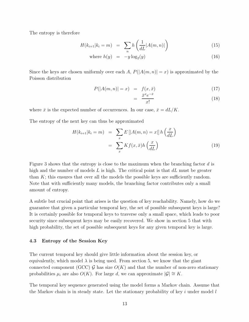
H(ki+1|ki = m) =∑
x
E [|A(m,n) = x|]h( x
dL
)
=∑
x
Kf(x, x̄)h( x
dL
)(19)
Figure 3 shows that the entropy is close to the maximum when the branching factor d is
high and the number of models L is high. The critical point is that dL must be greater
than K; this ensures that over all the models the possible keys are sufficiently random.
Note that with sufficiently many models, the branching factor contributes only a small
amount of entropy.
A subtle but crucial point that arises is the question of key reachability. Namely, how do we
guarantee that given a particular temporal key, the set of possible subsequent keys is large?
It is certainly possible for temporal keys to traverse only a small space, which leads to poor
security since subsequent keys may be easily recovered. We show in section 5 that with
high probability, the set of possible subsequent keys for any given temporal key is large.
4.3 Entropy of the Session Key
The current temporal key should give little information about the session key, or
equivalently, which model λ is being used. From section 5, we know that the giant
connected component (GCC) G has size O(K) and that the number of non-zero stationary
probabilities μi are also O(K). For large d, we can approximate |G| ∼= K.
The temporal key sequence generated using the model forms a Markov chain. Assume that
the Markov chain is in steady state. Let the stationary probability of key i under model l
13

62 64 6657
58
59
60
61
62
63
64
Number of Models (bits)
En
tro
py
Entropy of Next 64−bit Key for Various Branching Factors
d = 2d = 4d = 8d = 16
Figure 3. Entropy of next key given the current key. The Markov model is not knownto the adversary. K = 264.
be μli. Then the entropy of the model given the current temporal key ki is
H(l|ki) =∑
l
h
(μl
i∑l μ
li
)(20)
We note from experiment that the stationary probabilities are well approximated by a
Rayleigh distribution when d is small and a normal distribution when d is large (figures 4
and 5, respectively). In the experiment, we assumed K = L = 1024 and used the Mersenne
Twister as the PRNG.
Figure 6 shows that the model entropy is close to the maximum when the branching
probability is high and the number of models L is high. Increasing the branching factor
improves the model entropy.
14

0 1 2 3 4 5 6 7 8
x 10−3
0
50
100
150
200
250
300
350
400
Stationary Probability
Den
sity
Distribution of Stationary Probabilities (d = 4)
ObservedRayleigh PDF
Figure 4. Distribution of stationary probabilities is well approximated with Rayleighdistribution for small d.
0.5 1 1.5 2 2.5 3 3.5
x 10−3
0
100
200
300
400
500
600
Stationary Probability
Den
sity
Distribution of Stationary Probabilities (d = 32)
ObservedGaussian PDF
Figure 5. Distribution of stationary probabilities is well approximated with Gaussiandistribution for large d.
15

2 3 4 58
8.5
9
9.5
10
10.5
11
Branching Factor (bits)
En
tro
py
Entropy of Model given Current Key
L = 512L = 1024L = 2048
Figure 6. Entropy of chosen model given current key for various numbers of possiblemodels L. Keyspace size is K = 210.
4.4 Entropy Rate
Since the GCC is strongly connected, it is irreducible. With high probability, random
digraphs are also aperiodic. An irreducible and aperiodic Markov chain converges to its
unique stationary distribution μ (16 ), and the resulting entropy rate is
H(K) = −∑
m,n∈GμmAmn logAmn ≤ log d (21)
with equality when a transition between keys m and n implies that Amn = 1/d. Thus,
entropy rate is maximized when future keys are equiprobable.
In comparison, in section 4.2, we showed that when the model is not known, the entropy of
the next key was shown to be high, near the entropy of the keyspace K.
Having a higher entropy rate is beneficial for security since a single model can generate
many unique temporal key sequences. (Consider the multiplicity of paths that arise when d
is increased from 1.) This, in turn, makes it more difficult for the adversary to determine
which model is being used. She may try to use the Baum-Welch algorithm to determine
the underlying model, but the estimated parameters are not accurate unless the number of
observations is very high with respect to size of the state space (17 ). With a large
keyspace, it will take an infeasibly long time to make sufficient observations of each key.
16

5. Random Markov Model: Structure
Since we are using the Markov models for temporal key replacement, we are interested in
the structure of the pseudo-randomly generated model. Though the models are
deterministic given the particular PRNG used for generation, we assume for analysis that
they are statistically random and unpredictable (as discussed in section 4). Thus, without
fully specifying the model, which is infeasible for realistic key sizes, the structure of the
model is apparently random. We are therefore unable to guarantee certain properties of the
models, but we can make probabilistic statements. We say that an event occurs with high
probability when it occurs with probability 1 as K increases without bound.
In this section, we show that for any temporal key, the set of possible subsequent keys is
large. This property makes it infeasible for the adversary, given reasonable constraints on
her ability to perform a successful brute-force attack (i.e., test every key). In other words,
we never want to be in a situation where choosing a particular key limits the choices of
subsequent temporal keys.
In terms of graph theory, the reachable subspace for most keys in K should be large, that
is, O(K). A key v is reachable from u if there exists a (directed) path from u to v: u → v.
The reachable subspace for a key u is the set of all v for which u→ v.
First, we introduce the concept of strongly connected components. We use results from
graph theory to show that the size of a single GCC depends on the branching factor d
(18 ). Finally, we show that with probability 1, (a) all keys can reach the GCC and (b) no
keys leave the GCC. That is, the random Markov models are guaranteed to give highly
random key replacements.
5.1 Size of the GCC
We define some terms to facilitate the following discussion.
Definition 3 A digraph S is a strongly connected when there exists a directed path
between any randomly chosen pair of vertices u, v ∈ S:
u → v (22)
v → u (23)
Definition 4 The strongly connected components (SCCs) of a digraph are the maximal
strongly connected subgraphs. For a given digraph, the SCCs may be identified using
efficient algorithms such as Tarjan’s algorithm (19) or Gabow’s algorithm (20).
17

Definition 5 When the size of a SCC reaches O(K), it is typically referred to as the GCC
since it dominates the other SCCs in size.
The significance of the GCC is that for any given key in the GCC, it can reach any other
key of the GCC given enough transitions. When the GCC is large, this implies that there
are many keys that can be chosen in the future, which is good for security.
We outline the procedure of finding the GCC size and then give the results. We need the
following definitions to proceed. We outline the procedure of finding the GCC size and
then give the results. We need the following definitions to proceed. The fan-in of a node v
is the set of vertices u for which u→ v.
The fan-out of a node u is the set of nodes v for which u→ v. The fan-out (or fan-in) of a
vertex is large when its size is O(K). Let L+ be the set of vertices with a large fan-out,
and let L− be the set of vertices with a large fan-in.
Intuitively, when a node u has a large fan-out and a distinct node v �= u has a large fan-in,
the path u→ v exists with high probability. Thus, nodes that have both large fan-in and
large fan-out are likely to be connected (18). We highlight the relevant results below.
Let π− (resp., π+) be the probability that a randomly chosen vertex has a large fan-in
(resp., large fan-out). It follows that |L−| = π−K and |L+| = π+K. They are the smallest
non-negative solutions of
1 − π− =∑
i
p−i (1 − π−)i (24)
1 − π+ =∑
i
p+i (1 − π+)i (25)
where p−i (resp., π+) is the probability that a key has exactly i incoming (resp., outgoing)
transitions. These probabilities are calculated as
p−i =
(K
i
)pi(1 − p)K−i (26)
p+i =
{1 i = d0 otherwise
(27)
where p is the probability that there exists a transition between a randomly chosen pair of
current and next keys. Since each vertex has constant out-degree d, we have p = d/K, and
so the in-degree distribution is given by the binomial probability mass function with
parameter p.
When d > 1, π− has a unique solution in (0, 1), and π+ = 1. In other words, a positive
fraction of vertices have large fan-in while all vertices have large fan-out (i.e., |L+| = K.
18
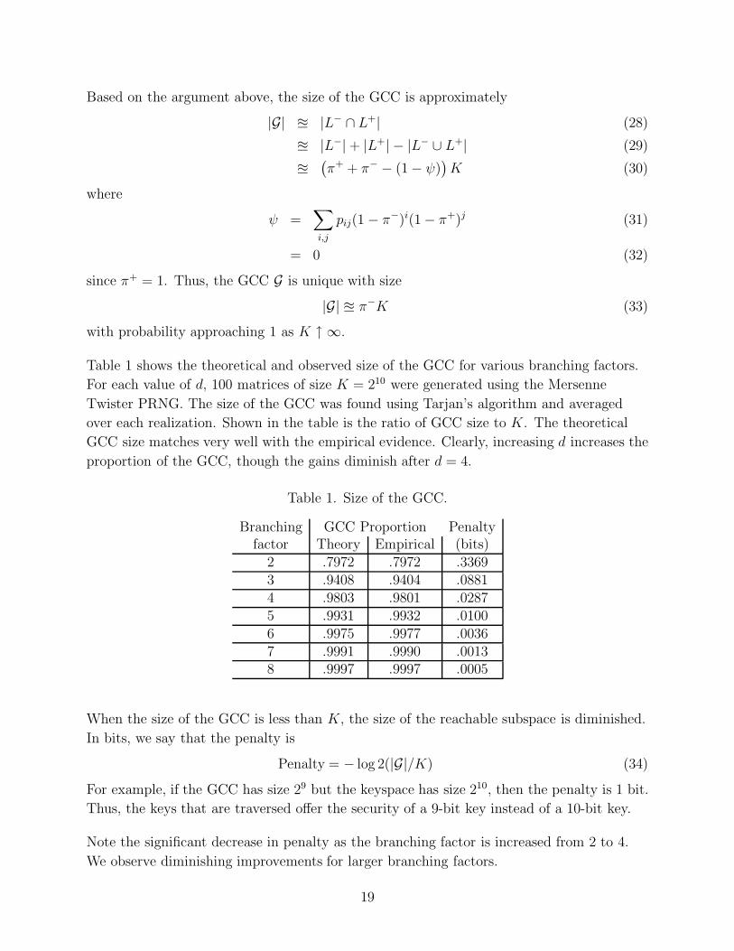
Based on the argument above, the size of the GCC is approximately
|G| � |L− ∩ L+| (28)
� |L−| + |L+| − |L− ∪ L+| (29)
�
(π+ + π− − (1 − ψ)
)K (30)
where
ψ =∑i,j
pij(1 − π−)i(1 − π+)j (31)
= 0 (32)
since π+ = 1. Thus, the GCC G is unique with size
|G| � π−K (33)
with probability approaching 1 as K ↑ ∞.
Table 1 shows the theoretical and observed size of the GCC for various branching factors.
For each value of d, 100 matrices of size K = 210 were generated using the Mersenne
Twister PRNG. The size of the GCC was found using Tarjan’s algorithm and averaged
over each realization. Shown in the table is the ratio of GCC size to K. The theoretical
GCC size matches very well with the empirical evidence. Clearly, increasing d increases the
proportion of the GCC, though the gains diminish after d = 4.
Table 1. Size of the GCC.
Branching GCC Proportion Penaltyfactor Theory Empirical (bits)
2 .7972 .7972 .33693 .9408 .9404 .08814 .9803 .9801 .02875 .9931 .9932 .01006 .9975 .9977 .00367 .9991 .9990 .00138 .9997 .9997 .0005
When the size of the GCC is less than K, the size of the reachable subspace is diminished.
In bits, we say that the penalty is
Penalty = − log 2(|G|/K) (34)
For example, if the GCC has size 29 but the keyspace has size 210, then the penalty is 1 bit.
Thus, the keys that are traversed offer the security of a 9-bit key instead of a 10-bit key.
Note the significant decrease in penalty as the branching factor is increased from 2 to 4.
We observe diminishing improvements for larger branching factors.
19

5.2 Reachability of the GCC
Since the GCC G is large, any key k ∈ G has a reachable subspace with size O(K) by
definition. However, what about those keys that are not in G? In order to guarantee keys
that traverse a large space, we need to show that with high probability
• regardless of initial key, the key replacement algorithm eventually chooses members
of the GCC, and
• if the current temporal key is in the GCC, future replacement keys will remain in the
GCC.
First, observe that when a key leaves the GCC, it does not have a path that returns to the
GCC. To see why, suppose that the path G → v exists, where v /∈ G. If a path v → Gexists, then since G → v this implies that v ∈ G, which is a contradiction. In other words,
when the replacement key sequence transitions outside of the GCC, it can never return.
Therefore, we need to show that once a key from the GCC is chosen, keys outside the GCC
are never chosen in the future.
Let us term the keys that are not in G as external. Let G− be the set of external keys that
have a path to G and let G+ be the set of external keys that are reachable from G, i.e.,
G− = {u|u� G} (35)
G+ = {v|G � v} (36)
The resulting set B = G− ∪ G ∪ G+ forms a bowtie digraph as shown in figure 7. The bows
of the graph are formed by two wings: G+ = L+ ∩ L− and G− = L+ ∩ L−.
Recall that |L+| = K and hence L+ = K. Hence B = K, i.e., the bowtie graph encompasses
all vertices in the space. It follows that L+ = ∅ and therefore G− = ∅. Therefore, any
randomly chosen key is either in G+ or G.
The structure of B yields the following properties:
1. If a key is not in G, then it is in G+. Therefore, with probability 1, the current state
will eventually be in G. With probability approaching 1 as K ↑ ∞, any randomly
chosen key will enter the GCC.
2. Once a key is in the GCC, it will not depart since with probability approaching 1 as
K ↑ ∞, |G−| = 0.
20

GCC
G
G+ G-
Figure 7. An example bowtie digraph connected to the giant connected component G.G+ leads into G, G− emanates from G.
In terms of temporal keys, the structure of the random Markov model guarantees that each
temporal key can reach a large subset (O(K)) of the keyspace. Therefore, the temporal
keys that will be generated from our key exchange algorithm traverse a large space thus
making the task of the adversary difficult.
6. Extension: Imperfect Key Recovery
In section 3, we assumed that as long as one of the keys Bob tests is the correct key, he is
able to determine the correct key without error. This is a good approximation in most
applications, but in this section we determine the effects of detection error on the proposed
key replacement method.
Suppose that the ciphertext xi has been encrypted with key ki as in equation 1. When we
test a single key m, there are two cases where the key recovery fails.
1. Missed detection: the correct key is tested (m = ki) but fails the check with
probability 1 − p > 0:
ψ(xi, m = ki) =
{0 w.p. 1 − p1 w.p. p
(37)
2. False alarm: the wrong key is tested (m �= ki) but passes the check with probability
21

α > 0:
ψ(xi, m �= ki) =
{0 w.p. 1 − α1 w.p. α
(38)
Recall that the recovery performed by Bob (section 3.3) checks the validity of d keys. We
assume that the integrity checks have independent outcomes. Considering a set of d keys
where exactly one is correct, there are four possible types of outcomes.
1. The correct key passes the integrity check (all others fail). This occurs with
probability
Pr[Case 1] = p(1 − α)d−1 (39)
2. The wrong key passes the integrity check (all others fail). This occurs with
probability
Pr[Case 2] = (d − 1)(1 − p)α(1 − α)d−2 (40)
3. No keys pass the integrity check. This occurs with probability
Pr[Case 3] = (1 − p)(1 − α)d−1 (41)
4. Multiple keys pass the integrity check. This occurs with probability
Pr[Case 4] = 1 − Pr[Case 1, 2, or 3] (42)
Looking ahead to section 6.2, the probability of a correct detection (Pr[Case 1]) needs to
be sufficiently high, otherwise Alice and Bob will lose synchrony quickly. In the following
section, we modify the recovery algorithm to improve the detection probability in the midst
of errors.
6.1 Extended Recovery Algorithm
In general, a key is used to encrypt multiple messages during the same epoch. Rather than
determining the replacement key after a single message, consider how C messages can be
used to make the decision. For the key epoch i, we denote the encrypted messages by
x1i , x
2i , . . ..
We assume that the number of times each key passes the integrity check are independent.
Bob tallies the number of times a key passes the check over the C messages, and selects the
key that passed the most times. We assume that kai = kb
i and λb = λa so that Bob knows
the transition probabilities to the next key.
22

1. Find the set of possible keys from kbi : N = {n|A(kb
i , n) > 0}.2. For each key n ∈ N :
T [n] =C∑
c=1
ψ(xci+1, n) (43)
3. Select kbi+1 = arg maxn T [n]
The probability that the correct key will be detected c times out of C is given by the
binomial probability B(c, C, p), where p is the probability of the correct key passing the
integrity check. Similarly, for the incorrect keys the probability is B(c, C, α), where α is the
probability of an incorrect key passing the integrity check. Since the trials have
independent outcomes, the probability that Bob chooses the correct key is given by
p̃ = Pr[kbi+1 = ka
i+1] (44)
=
C∑c=1
B(c, C, p)
(c−1∑d=0
B(d, C, α)
)d−1
(45)
Aside from the detection and false alarm probabilities (p, α, respectively), the number of
messages C determines the detection probability p̃ of the correct key. Figure 8 shows that
the probability of choosing the wrong key falls exponentially as C increases. Further, the
test does not need to consider large C when the detection probability p is high.
23

Figure 8. Probability of choosing the incorrect key for various raw detection key proba-bilities p when α = 10−7. Extending the key replacement over multiple mes-sages encrypted with the same key improves the detection probability. Lowerp require more observations for good detection probability.
6.2 Synchronization Performance
The probability that Bob chooses the incorrect key is ε = 1 − p̃. Thus, the probability that
Alice and Bob lose synchrony at epoch n0 is
Pr(Lost at n0) = ε(1 − ε)n0−1 (46)
We are interested in the case when Alice and Bob maintain synchrony for at least n0 with a
certain probability. That is,
Pr(n0 > n) =∑n<n0
Pr(Lost at n0) (47)
= 1 − (1 − ε)n−1 (48)
n =log(1 − Pr(n0 > n))
log(1 − ε)(49)
For example, we calculate that when ε = 10−4, then with probability 99.99% Alice and Bob
remain synchronized for at least 9.2 ∗ 104 keys. Figure 9 shows the number of key
transitions before failure for various confidence levels.
24

Figure 9. Number of key transitions before failure for various confidences.
6.3 Extension Efficiency
When the recovery of the key is extended for C messages, the number of computations and
memory requirements necessarily increase.
Communication: As in section 3, no explicit key replacement messages are exchanged.
However, there is an increased delay since the key decision requires the receipt of C > 1
messages.
Computation: Since the computations are identical for each message, the considering keys
over multiple messages times increases the computations by a factor of C . The final step of
selecting the key with the largest score requires negligible computation.
The cost of running the PRNG does not change and is the same as in section 3.4.
Memory: The set of possible keys remains constant over the duration of the test, so there
is no additional cost. However, there is the need to keep the tally of how many times each
key passes the integrity checks. This requires log2(C) bits per key, or d log2(C) bits in
total. Note that there was no need to keep score when the integrity check is perfect
because exactly one key would satisfy the integrity check.
25

7. Related Work
We give a characterization of a few approaches towards key replacement and highlight their
differences with the proposed method.
One of the most trivial rekeying strategies has Alice and Bob using their session key to
seed a PRNG. Periodically, they update their keys by taking the next n digits as the new
temporal key. While this requires no extra communication, the security of this method is
weak—the new temporal keys have no more randomness than the session key used to seed
the PRNG. Once the PRNG is seeded, the sequence of temporal keys is completely
deterministic and hence vulnerable to attack. In fact, this rekeying strategy may be viewed
as a degenerate case of the proposed method with branching factor d = 1. For comparison,
the proposed method (with d > 1) adds key entropy during each rekey because of the
randomization (section 4.4).
A stronger method is to use a one-way‡ function with a nonce to generate the next key,
e.g., ki+1 = F (x, ki) with ki the current key, x the nonce, and F (·) the one-way function. In
order to recover this key, the receiver needs knowledge of the nonce—it can be encrypted
with the temporal key and transmitted. A weakness with this approach is that the
discovery of a temporal key reveals all subsequent keys. This also requires some bandwidth
to transmit the nonce. The proposed method uses Markov models to restrict the possible
nonces in order to avoid the use of nonces while also preventing subsequent keys from being
revealed.
Instead of using the session key to encrypt all the temporal keys, the idea behind hash
chains (21) is to derive past keys from future keys. In particular, the current temporal key
ki is calculated using the next key ki+1 and a one-way hash function F (·), i.e.,
ki = F (ki+1). Alice and Bob generate a chain of hash values derived from the same initial
key kn, and begin to use the key k0. To replace the key, they simply use the next key k1.
However, after n key replacements Alice and Bob need to resynchronize and generate
another hash chain. This is not a very big problem, however, since hash chains can be
computed very efficiently (22). A significant weakness of hash chains is that there is no
forward secrecy. Once a key is compromised, the revelation of all past keys is trivial due to
their deterministic dependencies. While this property makes the use hash chains less than
ideal for key replacement, hash chains have found interesting applications in routing
protocols in ad hoc networks (23).
‡A function is one-way when it is easy (feasible) to compute but hard (infeasible, given resource con-straints) to invert.
26

The “sign and MAC” (SIGMA) approach encompasses a large family of key exchange
protocols that build upon the well-known Diffie-Helman (DH) key agreement protocol (8,
9). Careful combinations of digital signatures and message authentication codes (MACs)
are used to provide the security basis for signature-based authenticated key exchange using
DH protocols (e.g., IKE [24]). Generally these protocols require at least three messages for
both parties to contribute entropy towards the new key, bind identities with signatures,
and authenticate each other. Each message is accompanied by the corresponding
computation, which can be expensive; modular exponentiation is not as cheap as
symmetric encryption or decryption.
Another well-known protocol is Kerberos (10) (based on the Needham-Shroeder shared-key
protocol [25]), which uses a trusted authentication server to facilitate key exchange. The
authentication server has session keys shared individually with Alice and Bob and creates
temporal keys for them to use among themselves. All the encryptions are symmetric and
are therefore cheap, but this protocol requires the exchange of more messages because Alice
and Bob need to interact with the authentication server. The biggest caveat, of course, is
the existence and cooperation of such an authentication server.
A summary of the requirements of the key replacement methods are shown in table 2. Note
that there is no method that is simultaneously low-complexity, independent of third
parties, and secure. The proposed key replacement method is conceptually simple and its
security depends on randomness of the underlying CSPRNG. The choice of CSPRNG
varies the computational requirements of the method.
Table 2. Comparison.
Method No. of Messages Computation Cost Third Party? SecuritySeeded PRNG 0 Low No LowHash Chains 0 Low No LowDiffie-Helman Variants 3+ High No HighKerberos 4 Low Yes HighProposed Method 0 Variable No High
27

8. Conclusion
We have introduced a novel rekeying method that exploits the randomness of Markov
models to efficiently provide fresh keys to the users. The method is shown to generate
highly random symmetric keys while remaining lightweight in terms of communication and
storage costs. The security of the method depends on the underlying CSPRNG and
generally is improved at the cost of increased computational requirements. We have also
demonstrated that the proposed method has perfect forward secrecy as well as resistance to
known-key attacks. Finally, we note that the usefulness of the method is not restricted to
keys, but to any variable that is changed in a synchronous manner. For example, this
method can apply to frequency-hopped communications systems to vary the hop set
ordering.
28
References
[1] Fumy, W.; Landock, P. Principles of Key Management. IEEE J Sel. Areas Commun.,
Jun 1993, 11 (5), 785–793.
[2] Maurer, U. M. Authentication Theory and Hypothesis Testing. IEEE Trans. Inf. The-
ory. Jul 2000, 46 (4), 1350–1356.
[3] Silverman, R. D. A Cost-Based Security Analysis of Symmetric and Asymmetric Key
Lengths; RSA Laboratories; Bulletin 13, Nov 2001.
[4] Miller, V. S. Use of Elliptic Curves in Cryptography. Lecture notes in Computer Sciences
(CRYPTO 85) 1985, 218, 417–426.
[5] Koblitz, N. Elliptic Curve Cryptosystems. Mathematics of Computation Jan 1987, 48
(177), 203–209.
[6] Rivest, R. L.; Shamir, A.; Adleman, L. A Method for Obtaining Digital Signatures and
Public-Key Cryptosystems. Communications of the ACM 1978, 21 (2), 120–126.
[7] Eschenauer, L.; Giligor, V. D. A Key-Management Scheme for Distributed Sensor Net-
works. In Proceedings of the 9th ACM Conference on Computer and Communications
Security, ACM Press, 2002, 41–47.
[8] Diffie, W.; Hellman, M. E. New Directions in Cryptography. IEEE Trans. Inf. Theory
Nov 1976, 22 (6), 644–654.
[9] Krawczyk, H. SIGMA: The ’SIGn-and-MAc’ Approach to Authenticated Diffie-Hellman
and Its Use in the IKE-Protocols. CRYPTO ; 2003, 400–425.
[10] MIT. Kerberos: The Network Authentication Protocol. [online]. Available:
http://web.mit.edu/Kerberos/, Oct 2007.
[11] van der Merwe, J.; Dawoud, D. S.; McDonald, S. A Survey on Peer-to-peer Key Man-
agement for Mobile Ad hoc Networks. ACM Comput. Surv. 2007, 39 (1).
[12] Menezes, A. J.; van Oorschot, P. C.; Vanstone, S. A. Handbook of Applied Cryptography.
CRC Press, 2001.
[13] Blum, L.; Blum, M.; Shub, M. A Simple Unpredictable Pseudo-Random Number Gen-
erator. SIAM Journal on Computing May 1986, 15, 364383.
29

[14] Kelsey, J.; Schneier, B.; Ferguson, N. Yarrow-160: Notes on the Design and Analy-
sis of the Yarrow Cryptographic Pseudorandom Number Generator. In Sixth Annual
Workshop on Selected Areas in Cryptography. Springer, 1999, 13–33.
[15] Saito, M.; Matsumoto, M. SIMD-Oriented Fast Mersenne Twister: a 128-bit Pseudoran-
dom Number Generator, Monte Carlo and Quasi-Monte Carlo Methods 2006. Springer
Berlin Heidelberg, 2008, pp. 607–622.
[16] Ross, Sheldon M. Stochastic Processes, New York: Wiley, 1996.
[17] Welch, Lloyd R. Hidden Markov Models and the Baum-Welch Algorithm. IEEE Infor-
mation Theory Society Newsletter Dec 2003, 53 (4), 1, 10–13.
[18] Cooper, Colin; Frieze, Alan. The Size of the Largest Strongly Connected Component
of a Random Digraph with a Given Degree Sequence. Combinatorics, Probability and
Computing May 2004, 13 (3), 319–337.
[19] Tarjan, Robert. Depth-first Search and Linear Graph Algorithms. SIAM Journal on
Computing 1972, 1 (2), 146–160.
[20] Cheriyan, J.; Mehlhorn, K. Algorithms for Dense Graphs and Networks on the Random
Access Computer. Algorithmica Jun 1996, 15 (6), 521–549.
[21] Lamport, Leslie. Password Authentication with Insecure Communication. Communica-
tions of the ACM 1981, 24 (11), 770772.
[22] Hu, Yih-Chun; Jakobsson, Markus; Perrig, Adrian. Efficient Constructions for One-way
Hash Chains. Proceedings of The International Conference on Applied Cryptography and
Network Security (ACNS 2005), New York, NY, USA, 2005, pp 423441.
[23] Hu, Yih-Chun; Perrig, Adrian; Johnson, David B. Ariadne: a Secure on-demand Rout-
ing Protocol for ad hoc Networks. Wireless Networks January 2005, 11 (12), 2138.
[24] Harkins, D.; Carrel, D. The Internet Key Exchange (IKE), RFC2409 (Proposed Stan-
dard), Internet Engineering Task Force, Nov. 1998, obsolete by RFC 4306, updated by
RFC 4109. [Online]. Available: http://www.ietf.org/rfc/rfc2409.txt.
[25] Needham, Roger; Schroeder, Michael. Using Encryption for Authentication in Large
Networks of Computers. Communications of the ACM 1978, 21, 993999.
30

31
NO. OF
COPIES ORGANIZATION
1 ADMNSTR
ELEC DEFNS TECHL INFO CTR
ATTN DTIC OCP
8725 JOHN J KINGMAN RD STE 0944
FT BELVOIR VA 22060-6218
1 US ARMY RSRCH DEV AND ENGRG CMND
ARMAMENT RSRCH DEV & ENGRG CTR
ARMAMENT ENGRG & TECHNLGY CTR
ATTN AMSRD AAR AEF T J MATTS
BLDG 305
ABERDEEN PROVING GROUND MD 21005-5001
1 US ARMY INFO SYS ENGRG CMND
ATTN AMSEL IE TD A RIVERA
FT HUACHUCA AZ 85613-5300
1 US GOVERNMENT PRINT OFF
DEPOSITORY RECEIVING SECTION
ATTN MAIL STOP IDAD J TATE
732 NORTH CAPITOL ST NW
WASHINGTON DC 20402
1 DIRECTOR
US ARMY RSRCH LAB
ATTN RDRL ROE V W D BACH
PO BOX 12211
RESEARCH TRIANGLE PARK NC 27709
7 US ARMY RSRCH LAB
ATTN IMNE ALC HRR MAIL & RECORDS MGMT
ATTN RDRL CIN A KOTT
ATTN RDRL CIN B SADLER
ATTN RDRL CIN T B RIVERA
ATTN RDRL CIN T P YU
ATTN RDRL CIO LL TECHL LIB
ATTN RDRK CIO LT TECHL PUB
ADELPHI MD 20783-1197

32
INTENTIONALLY LEFT BLANK.