Rare B Meson Decays With Omega Mesons · Rare B Meson Decays With Omega Mesons Lei Zhang Stanford Linear Accelerator Center Stanford University Stanford, CA 94309 SLAC-Report-821

SLAC-R-821

Rare B Meson Decays With Omega Mesons

Lei Zhang

Stanford Linear Accelerator Center

Stanford University Stanford, CA 94309

SLAC-Report-821

Prepared for the Department of Energy under contract number DE-AC02-76SF00515

Printed in the United States of America. Available from the National Technical Information Service, U.S. Department of Commerce, 5285 Port Royal Road, Springfield, VA 22161.

BABAR-THESIS-04/123

This document, and the material and data contained therein, was developed under sponsorship of the United States Government. Neither the United States nor the Department of Energy, nor the Leland Stanford Junior University, nor their employees, nor their respective contractors, subcontractors, or their employees, makes an warranty, express or implied, or assumes any liability of responsibility for accuracy, completeness or usefulness of any information, apparatus, product or process disclosed, or represents that its use will not infringe privately owned rights. Mention of any product, its manufacturer, or suppliers shall not, nor is it intended to, imply approval, disapproval, or fitness of any particular use. A royalty-free, nonexclusive right to use and disseminate same of whatsoever, is expressly reserved to the United States and the University.

Rare B Meson Decays with ω Mesons

by

Lei Zhang

B.E., University of Science and Technology of China, 1996

M.S., Institute of High Energy Physics, Beijing, 1999

A thesis submitted to the

Faculty of the Graduate School of the

University of Colorado in partial fulfillment

of the requirements for the degree of

Doctor of Philosophy

Department of Physics

2004

This thesis entitled:Rare B Meson Decays with ω Mesons

written by Lei Zhanghas been approved for the Department of Physics

William T. Ford

Prof. Thomas A. DeGrand

Date

The final copy of this thesis has been examined by the signatories, and we find thatboth the content and the form meet acceptable presentation standards of scholarly

work in the above mentioned discipline.

iii

Zhang, Lei (Ph.D., Physics)

Rare B Meson Decays with ω Mesons

Thesis directed by Prof. William T. Ford

Rare charmless hadronic B decays are particularly interesting because of their

importance in understanding the CP violation, which is essential to explain the matter-

antimatter asymmetry in our universe, and of their roles in testing the “effective” theory

of B physics. The study has been done with the BABAR experiment, which is mainly

designed for the study of CP violation in the decays of neutral B mesons, and secondarily

for rare processes that become accessible with the high luminosity of the PEP-II B

Factory.

In a sample of 89 million produced BB pairs on the BABAR experiment, we

observed the decays B0 → ωK0 and B+ → ωρ+ for the first time, made more precise

measurements for B+ → ωh+ and reported tighter upper limits for B → ωK∗ and B0 →

ωρ0. The branching fractions measured are B(B+ → ωπ+) = (5.5 ± 0.9 ± 0.5) × 10−6,

B(B+ → ωK+) = (4.8±0.8±0.4)×10−6, B(B0 → ωK0) = (5.9+1.6−1.3±0.5)×10−6, B(B0 →

ωK∗0) = (3.4+1.8−1.6±0.4)×10−6 (< 6.0×10−6), B(B+ → ωK∗+) = (3.5+2.5

−2.0±0.7)×10−6 (<

7.4 × 10−6), B(B0 → ωρ0) = (0.6+1.3−1.1 ± 0.4) × 10−6 (< 3.3 × 10−6), and B(B+ →

ωρ+) = (12.6+3.7−3.3 ± 1.6) × 10−6. We also measure time-integrated charge asymmetries

Ach(B+ → ωπ+) = 0.03 ± 0.16 ± 0.01, Ach(B+ → ωK+) = −0.09 ± 0.17 ± 0.01, and

Ach(B+ → ωρ+) = 0.05± 0.26± 0.02. For B+ → ωρ+ we also measure the longitudinal

polarization fraction fL(B+ → ωρ+) = 0.88+0.12−0.15 ± 0.03.

To my wife Yi Sun and my daughter Cindy.

Acknowledgements

I am very fortunate that lots of people have helped me so much that without

them I could not possibly come this far in my academic study and get this research

work done. It would take quite a few pages to name all of them, and I might not be

able to express my deepest appreciation to them all explicitly. Nevertheless, I owe a

great deal to the people who have supported me during various times.

First of all, I must gratefully acknowledge my advisor, Bill Ford, who has accepted

me as Ph.D. student and given me the opportunity to undertake my research as part

of the BABAR Collaboration. His enthusiasm, encouragement and endless support were

always what I could rely on when things looked pessimistic. It has been a great pleasure

to work him and it is hard for me to imagine that one could have a better advisor than

Bill. I would also like to thank Jim Smith for his helpful advice and guidance during

all the stages of this project. Discussions with him were so fruitful that I could end up

with nothing otherwise when the analysis went stalled many times. Whenever it looked

the hardest time to me, Jim and Bill were there to help.

It is a tremendous task requiring team effort for anyone to accomplish any achieve-

ment in this field, and I would like to thank Jean Roy for his early work on ωh+ analysis;

Mirna van Hoek for her great analysis tools, Q2BUser and Q2BFit; Paul Bloom for his

insightful discussions and initial setup on ωK∗ and ωρ analysis; Fred Blanc for his

invaluable help in different stages of the analysis. Thanks also to Phil, Corry, Keith,

Fabian, Ian, Josh, Ishani, and all other Colorado group members who have made it such

vi

a wonderful team to work with.

I am also very grateful to all the BABAR collaboration members who have made

this work possible and all the PEP-II staff who have provided us with excellent lumi-

nosity and machine conditions. I want to thank Conveners and members from Quasi-

Two-Body Charmless Analysis Working Group and many other AWGs of BABAR, for

their unending support and beneficial discussions throughout the whole work and my

special thanks go to Jim Olsen, Bill Ford, Adrian Bevan, Jim Smith, Erich Varnes,

Luca Cavoto. I also thank Wouter Verkerke and David Kirkby for their wonderful con-

tributions of RooFit packages, John Back for his helpful discussion on RooDircPdf,

Alex Olivas for his help on digi-embedding studies, Andrei Gritsan and LLuisa Maria

Mir for their valuable discussions on V V analysis, Shahram Rahatlou for his excellent

research and thesis. Other colleagues who help me a lot and to whom I owe a lot are:

Ming Chao, Jinlong Zhang, Wei Yang, Aidong Chen, Gerhard Raven, Nick Danielson,

and many more. Thanks should also go to my analysis review committee members,

Bob Cahn, Massimo Carpinelli, Sasha Telnov, Carlo Dallapiccola, Teela Marie Pulliam,

Haibo Li, the institutional reviewers and the PubBoard members for their timely re-

views, comments and final approvals. I want to thank Haibo again for being my best

friend and mentor for so many years.

I have spent one year at SLAC, which turned out to be a very happy experience,

and I could not leave without saying thanks to Vera Luth, the leader of Group C which

hosted me. I also need to thank the administrative and technical staff at SLAC, in

particular Anna Pacheco, Nuria Ayala, Charlotte Hee, who have saved me lots of time

and provided me with the best services. Life at SLAC was even more wonderful with

all my friends around the Bay Area and I had lots of fun with many of them, including:

Jiquan Guo (Stanford), Changjun Ma (SBC), Haiming Xu (Philips), Shunjiang Xu

(SUN), Wei Zhao (Stanford), Rita Chen (SUN). My thanks to all of them and their

families.

vii

Throughout years of study at University of Colorado at Boulder, I have constantly

received enlightenment and inspiration from many faculty members from the Depart-

ment of Physics and other departments and I express my gratitude to all of them and

particularly to Walter Wyss, Neil Ashby, Jim Shepard, Tom DeGrand, Uriel Nauenberg,

Hal Gabow, Roger King, Kenneth Anderson. I would like to thank Susan Thompson,

Kathy Oliver, Joe Hurst, Mary Dang and all the staff for their excellent work. Either on

campus, or around Boulder and Denver Metro area, lots of friends from many different

backgrounds make everyday part of excitements. I especially thank Madam Zhen Xia

for treating my daughter like her own granddaughter; Changying Li’s family for being

our best friend and neighbor for almost four years.

In spite of my best efforts, this work can not be done on time without generous

support from my committee, Bill Ford, Jim Smith, John Cumalat, Tom DeGrand, and

Yung-Cheng Lee, to whom I owe a very special debt.

My acknowledgements would not be nearly complete without mentioning my fam-

ily and relatives nearby or far apart. I must thank my parents for their timeless faith

in me and constant support to me; and I should also thank my two sisters, who, during

all the years I have been away from my parents, have showed the traditional merits of

being company to my parents and making them happier. I am extremely grateful to my

mother-in-law for her liberal help by taking care of my daughter many times. Lastly,

and most important, I want to thank my wonderful wife. She gave up her job in Beijing,

her hometown, where she never left before, to come with me for my study. She gave

me perpetual love, support and encouragement that helped to bring this project to its

successful completion.

viii

Contents

Chapter

1 Theory 1

1.1 Introduction . . . . . . . . . . . . . . . . . . . . . . . . . . . . . . . . . . 1

1.2 Fundamental Fermions and Interactions . . . . . . . . . . . . . . . . . . 3

1.3 Static Quark Model of Hadrons . . . . . . . . . . . . . . . . . . . . . . . 6

1.4 Decay of Resonance . . . . . . . . . . . . . . . . . . . . . . . . . . . . . 9

1.5 Electroweak Interactions and CP Violation . . . . . . . . . . . . . . . . 15

1.5.1 The CKM Matrix . . . . . . . . . . . . . . . . . . . . . . . . . . 18

1.5.2 CP Violation in B Decays . . . . . . . . . . . . . . . . . . . . . . 22

1.6 Hadronic B Decays . . . . . . . . . . . . . . . . . . . . . . . . . . . . . . 30

1.6.1 Decay Diagrams . . . . . . . . . . . . . . . . . . . . . . . . . . . 30

1.6.2 Low-Energy Effective Hamiltonians . . . . . . . . . . . . . . . . . 34

2 The BABAR Experiment 39

2.1 Introduction . . . . . . . . . . . . . . . . . . . . . . . . . . . . . . . . . . 39

2.2 The PEP-II B Factory . . . . . . . . . . . . . . . . . . . . . . . . . . . . 39

2.3 The BABAR Detector . . . . . . . . . . . . . . . . . . . . . . . . . . . . . 46

2.3.1 The Silicon Vertex Tracker (SVT) . . . . . . . . . . . . . . . . . 49

2.3.2 The Drift Chamber (DCH) . . . . . . . . . . . . . . . . . . . . . 54

2.3.3 DIRC . . . . . . . . . . . . . . . . . . . . . . . . . . . . . . . . . 60

ix

2.3.4 The Electromagnetic Calorimeter (EMC) . . . . . . . . . . . . . 63

2.3.5 The Instrumented Flux Return (IFR) . . . . . . . . . . . . . . . 68

2.3.6 The Trigger System . . . . . . . . . . . . . . . . . . . . . . . . . 75

2.3.7 The Data Acquisition (DAQ) and Online Computing System . . 77

3 Analysis Techniques 79

3.1 The BABAR Software and Analysis Tools . . . . . . . . . . . . . . . . . . 79

3.2 Data Sets . . . . . . . . . . . . . . . . . . . . . . . . . . . . . . . . . . . 87

3.3 Particle Reconstruction and Identification . . . . . . . . . . . . . . . . . 90

3.3.1 Charged Tracks . . . . . . . . . . . . . . . . . . . . . . . . . . . . 90

3.3.2 Neutral Particles . . . . . . . . . . . . . . . . . . . . . . . . . . . 91

3.3.3 Electron, Muon, and Proton Identification . . . . . . . . . . . . . 91

3.3.4 Kaon Identification . . . . . . . . . . . . . . . . . . . . . . . . . . 92

3.3.5 π0 Selection . . . . . . . . . . . . . . . . . . . . . . . . . . . . . . 95

3.3.6 K0S Selection . . . . . . . . . . . . . . . . . . . . . . . . . . . . . 96

3.4 B Daughter Selection . . . . . . . . . . . . . . . . . . . . . . . . . . . . 98

3.4.1 ω Selection . . . . . . . . . . . . . . . . . . . . . . . . . . . . . . 98

3.4.2 K/π Separation . . . . . . . . . . . . . . . . . . . . . . . . . . . . 101

3.4.3 K0S Selection . . . . . . . . . . . . . . . . . . . . . . . . . . . . . 105

3.4.4 K∗ Selection . . . . . . . . . . . . . . . . . . . . . . . . . . . . . 106

3.4.5 ρ Selection . . . . . . . . . . . . . . . . . . . . . . . . . . . . . . 107

3.4.6 Helicity Distributions . . . . . . . . . . . . . . . . . . . . . . . . 109

3.5 B Reconstruction . . . . . . . . . . . . . . . . . . . . . . . . . . . . . . . 118

3.5.1 ∆E and mES . . . . . . . . . . . . . . . . . . . . . . . . . . . . . 118

3.5.2 Continuum Background Suppression . . . . . . . . . . . . . . . . 121

3.5.3 BB Background . . . . . . . . . . . . . . . . . . . . . . . . . . . 126

3.6 Maximum Likelihood Fit . . . . . . . . . . . . . . . . . . . . . . . . . . . 131

x

3.6.1 K/π Fitting . . . . . . . . . . . . . . . . . . . . . . . . . . . . . . 134

3.6.2 fL Fitting . . . . . . . . . . . . . . . . . . . . . . . . . . . . . . . 137

3.6.3 Floating Continuum Background Parameters . . . . . . . . . . . 138

3.6.4 Fit Validation . . . . . . . . . . . . . . . . . . . . . . . . . . . . . 139

3.6.5 Signal Significance and Upper Limit . . . . . . . . . . . . . . . . 141

3.7 Systematic Errors . . . . . . . . . . . . . . . . . . . . . . . . . . . . . . . 141

3.7.1 Combining Results . . . . . . . . . . . . . . . . . . . . . . . . . . 145

4 Analysis Results 147

4.1 B+ → ωK+, ωπ+ and B0 → ωK0 . . . . . . . . . . . . . . . . . . . . . . 147

4.2 B → ωK∗ and B → ωρ . . . . . . . . . . . . . . . . . . . . . . . . . . . . 157

5 Conclusions 175

Bibliography 177

xi

Tables

Table

1.1 Quarks and leptons . . . . . . . . . . . . . . . . . . . . . . . . . . . . . . 4

1.2 Fundamental interactions . . . . . . . . . . . . . . . . . . . . . . . . . . 4

1.3 Light pseudoscalar mesons and vector mesons . . . . . . . . . . . . . . . 7

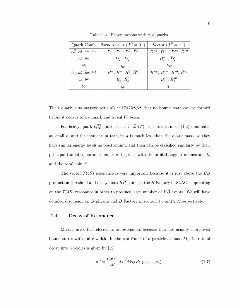
1.4 Heavy mesons with c, b quarks. . . . . . . . . . . . . . . . . . . . . . . . 9

1.5 Angular distributions of two-body pseudoscalar decays . . . . . . . . . . 13

1.6 Light meson decays . . . . . . . . . . . . . . . . . . . . . . . . . . . . . . 14

1.7 Theoretical predictions and previous measurements . . . . . . . . . . . 38

2.1 The production cross-sections of e+e− at√s = 10.58 GeV . . . . . . . . 41

2.2 The PEP-II beam parameters as of June 2004 . . . . . . . . . . . . . . . 43

2.3 Subsystems of the BABAR detector . . . . . . . . . . . . . . . . . . . . . 49

2.4 Properties of CsI(Tl) . . . . . . . . . . . . . . . . . . . . . . . . . . . . . 65

2.5 Event rates for the principal physics processes . . . . . . . . . . . . . . . 75

3.1 Summary of signal Monte Carlo samples used for different modes . . . . 88

3.2 List of non-default package versions for Ntuple production . . . . . . . . 89

3.3 Electron identification selectors . . . . . . . . . . . . . . . . . . . . . . . 92

3.4 Proton LH selectors . . . . . . . . . . . . . . . . . . . . . . . . . . . . . 93

3.5 Corrections on ω mass . . . . . . . . . . . . . . . . . . . . . . . . . . . . 99

3.6 K∗/ρ H cuts applied to V V modes . . . . . . . . . . . . . . . . . . . . . 117

xii

3.7 cos θT cuts . . . . . . . . . . . . . . . . . . . . . . . . . . . . . . . . . . . 124

3.8 Dominant BB background modes for B → ωK∗ . . . . . . . . . . . . . . 128

3.9 Dominant BB background modes for B → ωρ . . . . . . . . . . . . . . . 129

3.10 Average number of candidate per event . . . . . . . . . . . . . . . . . . 132

4.1 Numbers of charmless B background events for PV modes . . . . . . . . 148

4.2 Toy study with charmless BB MC sample for PV modes . . . . . . . . 148

4.3 Summary of pure toy fits for PV modes . . . . . . . . . . . . . . . . . . 149

4.4 Summary of embedded toy fits for PV modes . . . . . . . . . . . . . . . 151

4.5 ML fit results for B+ → ωK+, ωπ+, and B0 → ωK0 . . . . . . . . . . . 152

4.6 Systematic errors for B+ → ωK+, ωπ+, and B0 → ωK0 . . . . . . . . . 155

4.7 Detailed ML fit yield systematic errors for PV modes . . . . . . . . . . 156

4.8 Summary of pure toy fits for V V modes with fixed fL . . . . . . . . . . 158

4.9 Summary of embedded toy fits for V V modes with fixed fL . . . . . . . 158

4.10 Expected sensitivities for V V modes . . . . . . . . . . . . . . . . . . . . 159

4.11 Summary of pure toy fits for B+ → ωρ+ with floated fL . . . . . . . . . 160

4.12 Summary of embedded toy fits for B+ → ωρ+ with floated fL . . . . . . 160

4.13 ML fit results for B+ → ωK∗+ and B0 → ωK∗0 . . . . . . . . . . . . . . 164

4.14 ML fit results for B+ → ωρ+ and B0 → ωρ0 . . . . . . . . . . . . . . . . 165

4.15 Systematic errors for B → ωK∗ and B → ωρ . . . . . . . . . . . . . . . 170

4.16 Detailed ML fit yield systematic errors for V V modes . . . . . . . . . . 171

xiii

Figures

Figure

1.1 C, P , and CP operations on neutrino and antineutrino . . . . . . . . . . 3

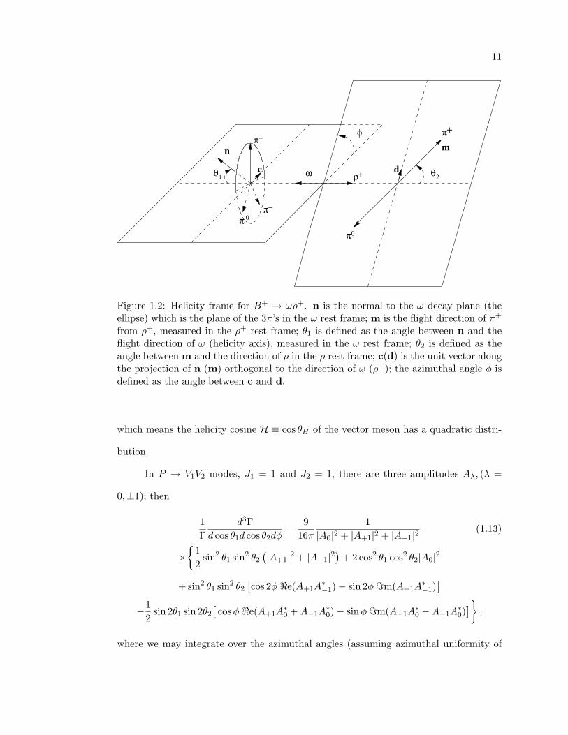
1.2 Helicity frame for B+ → ωρ+ . . . . . . . . . . . . . . . . . . . . . . . . 11

1.3 Angular distribution of P → V V decays . . . . . . . . . . . . . . . . . . 12

1.4 Unitarity triangles . . . . . . . . . . . . . . . . . . . . . . . . . . . . . . 19

1.5 Rescaled Unitarity Triangle . . . . . . . . . . . . . . . . . . . . . . . . . 21

1.6 Feynman diagram describing B0 – B0 mixing. . . . . . . . . . . . . . . . 25

1.7 CP violation in interference between mixing and decay . . . . . . . . . . 27

1.8 Quark diagrams describing b decays . . . . . . . . . . . . . . . . . . . . 32

1.9 Feynman diagrams for rare B decays . . . . . . . . . . . . . . . . . . . . 33

1.10 Feynman diagrams for decays B → ωh2 . . . . . . . . . . . . . . . . . . 35

2.1 e+e− hadronic cross-section at the Υ resonances . . . . . . . . . . . . . 40

2.2 The Linac, PEP-II storage rings, and the location of the BABAR detector. 42

2.3 Schematic view of the interaction region . . . . . . . . . . . . . . . . . . 43

2.4 The PEP-II integrated luminosity . . . . . . . . . . . . . . . . . . . . . . 44

2.5 Longitudinal section of the BABAR detector . . . . . . . . . . . . . . . . 47

2.6 Forward end view of the BABAR detector . . . . . . . . . . . . . . . . . . 48

2.7 Schematic view of the longitudinal section of SVT . . . . . . . . . . . . 50

2.8 Schematic view of the transverse section of SVT . . . . . . . . . . . . . 51

xiv

2.9 z and φ hit resolutions of SVT . . . . . . . . . . . . . . . . . . . . . . . 53

2.10 Longitudinal section of the DCH . . . . . . . . . . . . . . . . . . . . . . 55

2.11 DCH cell layout . . . . . . . . . . . . . . . . . . . . . . . . . . . . . . . . 56

2.12 Track parameter resolutions . . . . . . . . . . . . . . . . . . . . . . . . . 57

2.13 Tracking efficiency of the DCH . . . . . . . . . . . . . . . . . . . . . . . 58

2.14 Resolution of transverse momentum . . . . . . . . . . . . . . . . . . . . 59

2.15 dE/dx as a function of track momentum . . . . . . . . . . . . . . . . . . 59

2.16 Schematics of the DIRC fused silica radiator bar and imaging region . . 61

2.17 Transverse cross-section of a DIRC bar box . . . . . . . . . . . . . . . . 61

2.18 DIRC PMT hits . . . . . . . . . . . . . . . . . . . . . . . . . . . . . . . 63

2.19 DIRC π/K separation . . . . . . . . . . . . . . . . . . . . . . . . . . . . 64

2.20 Distribution of measured Cerenkov angle θc . . . . . . . . . . . . . . . . 64

2.21 Longitudinal cross-section of the top half of EMC . . . . . . . . . . . . . 66

2.22 Schematics of a wrapped CsI(Tl) crystal of the EMC . . . . . . . . . . . 67

2.23 EMC energy resolution as a function of the shower energy . . . . . . . . 69

2.24 EMC angular resolution as a function of the shower energy . . . . . . . 69

2.25 EMC electron efficiency and pion misidentification probability . . . . . . 70

2.26 Overview of the IFR . . . . . . . . . . . . . . . . . . . . . . . . . . . . . 71

2.27 Cross section of a planar RPC . . . . . . . . . . . . . . . . . . . . . . . . 72

2.28 Muon efficiency and pion misidentification rates of IFR . . . . . . . . . 74

2.29 Schematic diagram of the BABAR DAQ system . . . . . . . . . . . . . . 78

3.1 Invariant mass Mγγ for π0 candidates . . . . . . . . . . . . . . . . . . . 96

3.2 Invariant mass Mπ+π− for K0S candidates . . . . . . . . . . . . . . . . . 97

3.3 Distributions of invariant mass Mπ+π−π0 for ω candidates . . . . . . . . 100

3.4 DIRC pull distributions for K/π . . . . . . . . . . . . . . . . . . . . . . 102

xv

3.5 DIRC pull distributions for off-peak data, corrected, and uncorrected

continuum MC . . . . . . . . . . . . . . . . . . . . . . . . . . . . . . . . 104

3.6 Scattered plot of DIRC pulls distributions for K/π hypotheses . . . . . 105

3.7 Distributions of invariant mass MKπ for K∗ candidates . . . . . . . . . 108

3.8 Distributions of invariant mass Mππ for ρ candidates . . . . . . . . . . . 110

3.9 H distributions of P → PV decays . . . . . . . . . . . . . . . . . . . . . 112

3.10 2D signal H distributions for P → V V decays with acceptance effects . 114

3.11 Roll-off effects of H distributions . . . . . . . . . . . . . . . . . . . . . . 115

3.12 Background H distributions for P → V V decays . . . . . . . . . . . . . 117

3.13 ∆E distributions . . . . . . . . . . . . . . . . . . . . . . . . . . . . . . . 120

3.14 mES distributions . . . . . . . . . . . . . . . . . . . . . . . . . . . . . . . 120

3.15 Typical BB event and qq event . . . . . . . . . . . . . . . . . . . . . . . 122

3.16 Thrust angle cos θT distributions for BB signal and qq background . . . 123

3.17 Fisher distributions for signal and continuum background . . . . . . . . 125

3.18 BB background PDFs . . . . . . . . . . . . . . . . . . . . . . . . . . . . 130

3.19 ∆E distributions for K/π . . . . . . . . . . . . . . . . . . . . . . . . . . 135

3.20 2D plots δ∆E and δS vs Plab . . . . . . . . . . . . . . . . . . . . . . . . 135

3.21 Distributions of δ∆E and δS . . . . . . . . . . . . . . . . . . . . . . . . 136

4.1 Pure toy signal yield distributions for B+ → ωh+ . . . . . . . . . . . . . 150

4.2 Pure toy signal yield distribution for B0 → ωK0 . . . . . . . . . . . . . 150

4.3 mES and ∆E projection plots for B+ → ωπ+, ωK+, and B0 → ωK0 . . 153

4.4 Goodness-of-fit plots for B+ → ωh+ and B0 → ωK0 . . . . . . . . . . . 154

4.5 fL distributions from toy studies for B+ → ωρ+ (fL ∈ [0, 1]) . . . . . . . 161

4.6 fL distributions from toy studies for B+ → ωρ+ (no physical limits) . . 162

4.7 Combining decay sub-modes of B+ → ωK∗+ . . . . . . . . . . . . . . . 163

4.8 mES and ∆E projection plots for B → ωK∗ and B → ωρ . . . . . . . . 166

xvi

4.9 Contour plots fL vs signal yield and fL vs B for B+ → ωρ+ . . . . . . . 167

4.10 Correlation between ρ mass and helicity . . . . . . . . . . . . . . . . . . 168

4.11 Goodness-of-fit plots for B → ωK∗ and B → ωρ . . . . . . . . . . . . . 169

4.12 mES and ∆E sPlots for B+ → ωρ+ . . . . . . . . . . . . . . . . . . . . . 172

4.13 Mω and Mρ sPlots for B+ → ωρ+ . . . . . . . . . . . . . . . . . . . . . 173

4.14 Hω/ρ sPlots for B+ → ωρ+ . . . . . . . . . . . . . . . . . . . . . . . . . 173

4.15 F sPlots for B+ → ωρ+ . . . . . . . . . . . . . . . . . . . . . . . . . . . 174

Chapter 1

Theory

1.1 Introduction

People’s desire to understand the structure of matter is never ending, and it

is now well known that matter is built from molecules and atoms which in turn are

made from nucleons and electrons. These subatomic particles are called elementary

particles which are not necessarily truly elementary. Particle physics deals with such

elementary particles and the interactions of these particles. The discovery of the electron

by J. J. Thomson in 1897 [1] marked the first discovery of the elementary particles, and

in the next 50 years many new particles were discovered, mainly from cosmic rays.

Particle physics came into a new era after the development of high energy acceler-

ators and detectors, which provided intense and controlled beams and precise measure-

ments of particles produced by collision. Modern experiments on particle physics are a

challenge both to technology and human collaboration. In Chapter 2 we will describe

one such particle physics experiment where this work has been done.

This chapter serves as a short review of our current knowledge in particle physics

most relevant to this work; for a general introduction to the subject of particle physics,

see for example Ref. 9. A very important concept in physics is symmetries and con-

servation laws. Symmetry properties or invariance principles under transformations

are connected with conservation laws. For example, invariance of a system under spa-

tial translations corresponds to conservation of momentum, and invariance under time

2

translations corresponds to conservation of energy.

Three discrete transformations, charge conjugation C, parity (spatial reflection)

P , and time reversal T , are of particular interest in particle physics. While the laws of

classical mechanics and electrodynamics are invariant under these discrete transforma-

tions, experimental evidence showed violations of these operations in weak interactions.

P violation was first suggested by T. D. Lee and C. N. Yang [2] in 1956 and observed

by C. Wu et al. [3] the next year. C violation was indicated by the measurement of

neutrino helicity, which is left-handed for neutrinos and right-handed for antineutrinos,

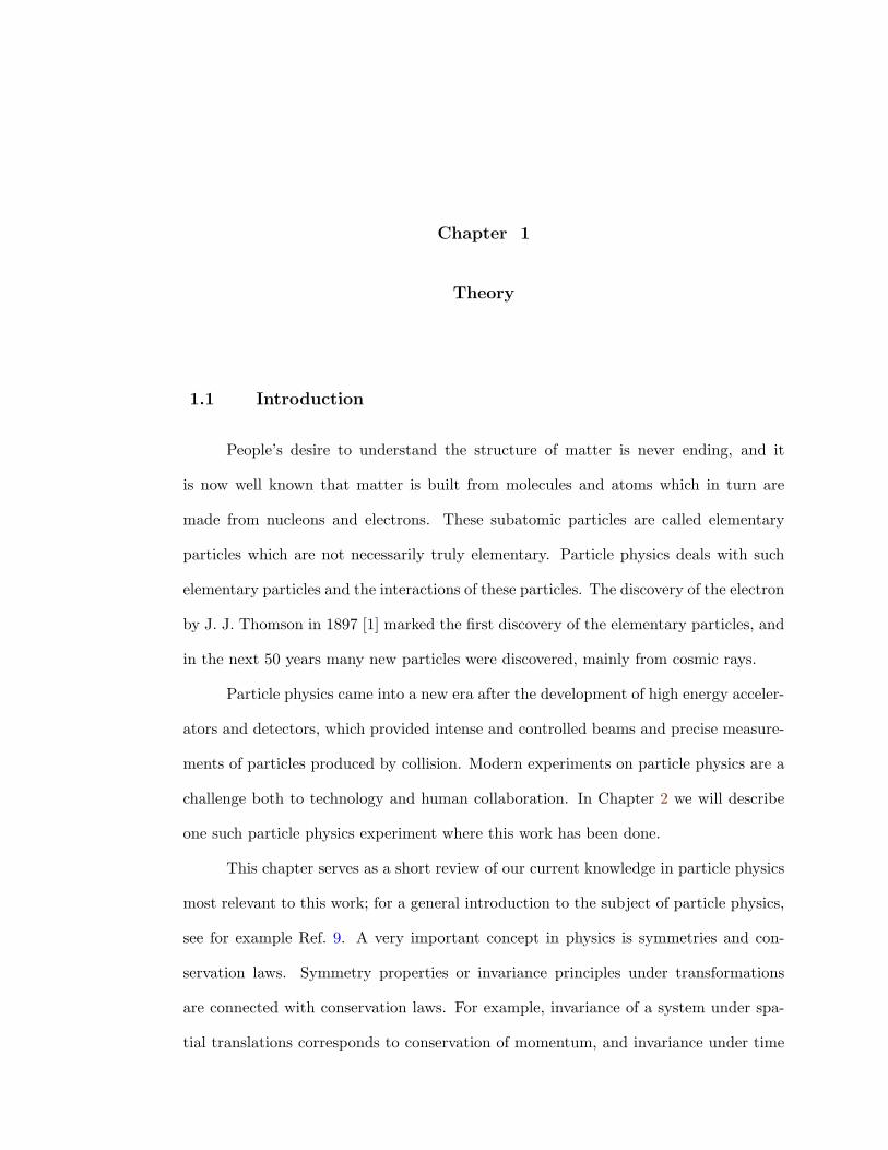
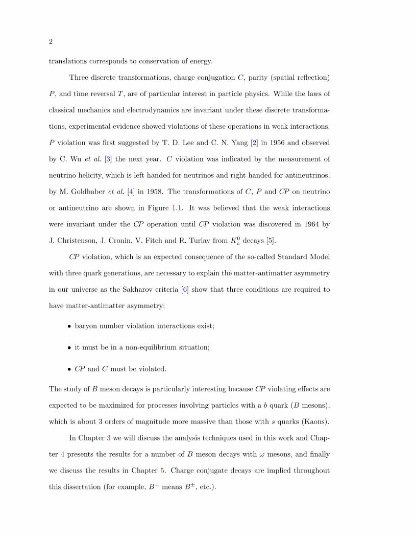
by M. Goldhaber et al. [4] in 1958. The transformations of C, P and CP on neutrino

or antineutrino are shown in Figure 1.1. It was believed that the weak interactions

were invariant under the CP operation until CP violation was discovered in 1964 by

J. Christenson, J. Cronin, V. Fitch and R. Turlay from K0L decays [5].

CP violation, which is an expected consequence of the so-called Standard Model

with three quark generations, are necessary to explain the matter-antimatter asymmetry

in our universe as the Sakharov criteria [6] show that three conditions are required to

have matter-antimatter asymmetry:

• baryon number violation interactions exist;

• it must be in a non-equilibrium situation;

• CP and C must be violated.

The study of B meson decays is particularly interesting because CP violating effects are

expected to be maximized for processes involving particles with a b quark (B mesons),

which is about 3 orders of magnitude more massive than those with s quarks (Kaons).

In Chapter 3 we will discuss the analysis techniques used in this work and Chap-

ter 4 presents the results for a number of B meson decays with ω mesons, and finally

we discuss the results in Chapter 5. Charge conjugate decays are implied throughout

this dissertation (for example, B+ means B±, etc.).

3

p

LH neutrino

P

RH neutrinoNot exist

p

RH antineutrino

p

C

p

LH antineutrinoNot exist

C

P

CP

s

s

s

s

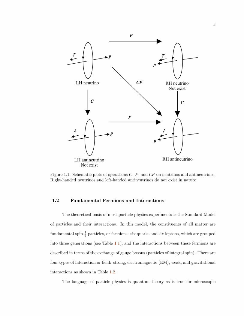
Figure 1.1: Schematic plots of operations C, P , and CP on neutrinos and antineutrinos.Right-handed neutrinos and left-handed antineutrinos do not exist in nature.

1.2 Fundamental Fermions and Interactions

The theoretical basis of most particle physics experiments is the Standard Model

of particles and their interactions. In this model, the constituents of all matter are

fundamental spin 12 particles, or fermions: six quarks and six leptons, which are grouped

into three generations (see Table 1.1), and the interactions between these fermions are

described in terms of the exchange of gauge bosons (particles of integral spin). There are

four types of interaction or field: strong, electromagnetic (EM), weak, and gravitational

interactions as shown in Table 1.2.

The language of particle physics is quantum theory as is true for microscopic

4

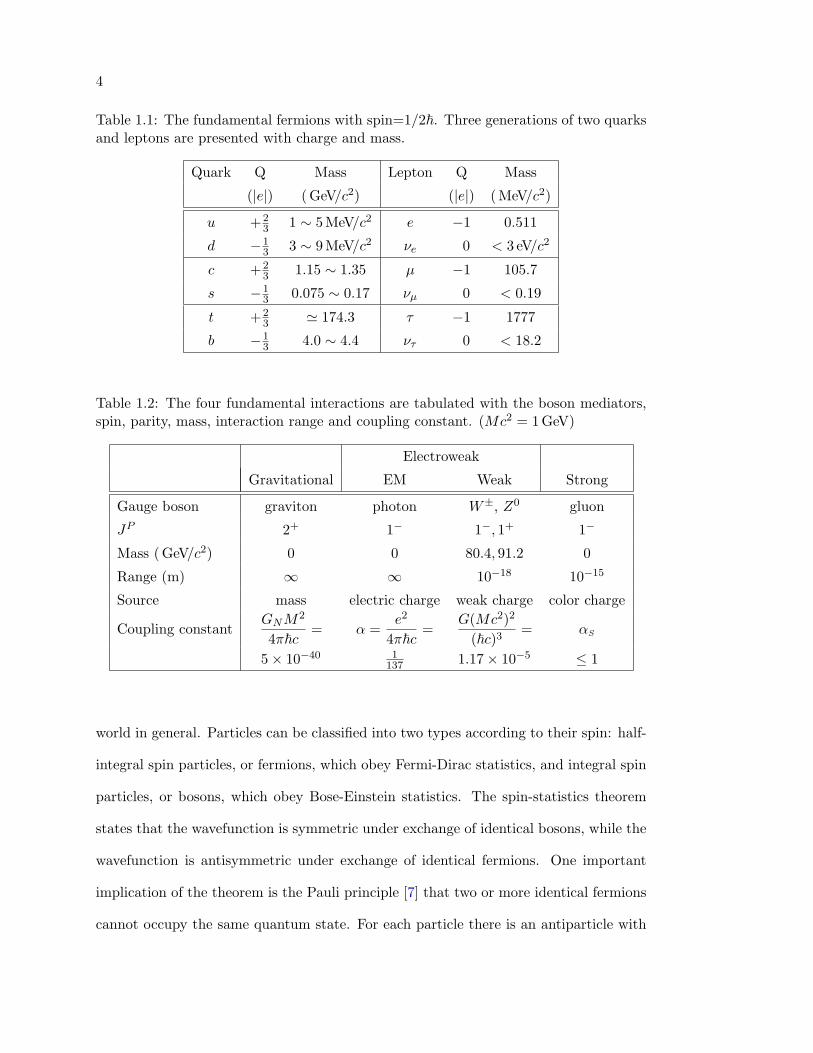
Table 1.1: The fundamental fermions with spin=1/2~. Three generations of two quarksand leptons are presented with charge and mass.

Quark Q Mass Lepton Q Mass

(|e|) (GeV/c2) (|e|) (MeV/c2)

u +23 1 ∼ 5 MeV/c2 e −1 0.511

d −13 3 ∼ 9 MeV/c2 νe 0 < 3 eV/c2

c +23 1.15 ∼ 1.35 µ −1 105.7

s −13 0.075 ∼ 0.17 νµ 0 < 0.19

t +23 ' 174.3 τ −1 1777

b −13 4.0 ∼ 4.4 ντ 0 < 18.2

Table 1.2: The four fundamental interactions are tabulated with the boson mediators,spin, parity, mass, interaction range and coupling constant. (Mc2 = 1GeV)

Electroweak

Gravitational EM Weak Strong

Gauge boson graviton photon W±, Z0 gluon

JP 2+ 1− 1−, 1+ 1−

Mass (GeV/c2) 0 0 80.4, 91.2 0

Range (m) ∞ ∞ 10−18 10−15

Source mass electric charge weak charge color charge

Coupling constantGNM

2

4π~c= α =

e2

4π~c=

G(Mc2)2

(~c)3= αS

5× 10−40 1137 1.17× 10−5 ≤ 1

world in general. Particles can be classified into two types according to their spin: half-

integral spin particles, or fermions, which obey Fermi-Dirac statistics, and integral spin

particles, or bosons, which obey Bose-Einstein statistics. The spin-statistics theorem

states that the wavefunction is symmetric under exchange of identical bosons, while the

wavefunction is antisymmetric under exchange of identical fermions. One important

implication of the theorem is the Pauli principle [7] that two or more identical fermions

cannot occupy the same quantum state. For each particle there is an antiparticle with

5

the same mass and lifetime but with opposite charge, and fermions and antifermions

can only be created or destroyed in pairs.

The leptons carry integral charge, −|e|, and the neutral leptons are called neutri-

nos. Leptons are grouped into pairs, electron e and electron neutrino νe, muon µ and

muon neutrino νµ, tau τ and tau neutrino ντ . The quarks carry fractional charge, +23 |e|

or −13 |e|. The type of quark is called the flavor of quark and is donated by a letter for

each ‘flavor’: u for ‘up’, d for ‘down’, s for ‘strange’, c for ‘charmed’, b for ‘bottom’ and

t for ‘top’. Just like leptons, the quarks are grouped into three generations: u and d, s

and c, b and t. Leptons can exist as free particles, but quarks are confined in hadrons

and single quarks as free particles have not been observed.

The interactions between particles are described in quantum field theory through

the exchange of particular bosons associated with the interactions. As is shown in

Table 1.2, gravitational interactions are the weakest force among all the fundamental

interactions and have negligible effect on current experiments of particle physics. It is a

long-range interaction mediated by exchange of spin 2 boson, the graviton, which must

have no mass.

Electromagnetic interactions are mediated by photon (γ) exchange between charged

particles as described in quantum electrodynamics (QED). The coupling constant of

electromagnetic interactions, α ∼ 1137 , specifies the strength of the interaction. The

photon has no mass so the electromagnetic interactions are long-range interactions.

Weak interactions take place between all quarks and leptons, mediated by the

massive W± and Z0 bosons, which couple to fermions with g and g′, respectively. At

low momentum transfer, q2 M2W , the weak coupling mediated by W± can be written

asG√2

=g2

8M2W

=e2

8 sin2 θWM2W

, (1.1)

where θW is the weak mixing angle with sin2 θW ' 0.22, and MW = 80.4 GeV/c2 is

6

the mass of W boson. G/√

2 is about 10−3α, so the weak interactions are drowned

by strong and electromagnetic interactions unless these interactions are forbidden by

some conservation laws. Since the mediators of weak interactions also have mass, the

interactions have very short range.

The weak and electromagnetic interactions can be unified through the electro-

weak theory proposed by Glashow, Weinberg and Salam [8], and we will discuss the

electroweak interactions at length in section 1.5 for the importance of the theory to this

work.

Strong interactions take place between quarks, and the interquark force is me-

diated by a massless boson, the gluon. In the theory of strong interactions, quantum

chromodynamics (QCD), the source of interactions is six types of ‘color charge’. A

quark carries one of the three basic colors (red r, blue b, and green g) and antiquark

carries anticolors (r, b, and g). Gluons carry one color and one anti-color and form

an octet of active states: rb, rg, bg, br, gr, gb, 1√2(rr − bb), 1√

6(rr + bb− 2gg). The QCD

potential has the form of

V = −43αS

r+ kr . (1.2)

At high q2 (or small distance), where the first term dominates, single-gluon exchange

is a good approximation, while at low q2 (or large distance), where the second term

dominates, the force increases indefinitely resulting in the color confinement of quarks

and gluons inside hadrons. Thus there only exist color singlet bound states of quarks

and antiquarks. The colorless quark combinations with lowest energy are the qqq states

(baryons, for example, proton and neutron) and qq (mesons, for example, kaon, pion).

1.3 Static Quark Model of Hadrons

Though a dynamic structure of hadrons, as in the theory of QCD, and observed

by experiments including lepton-nucleon scattering, is a collection of valence quarks,

7

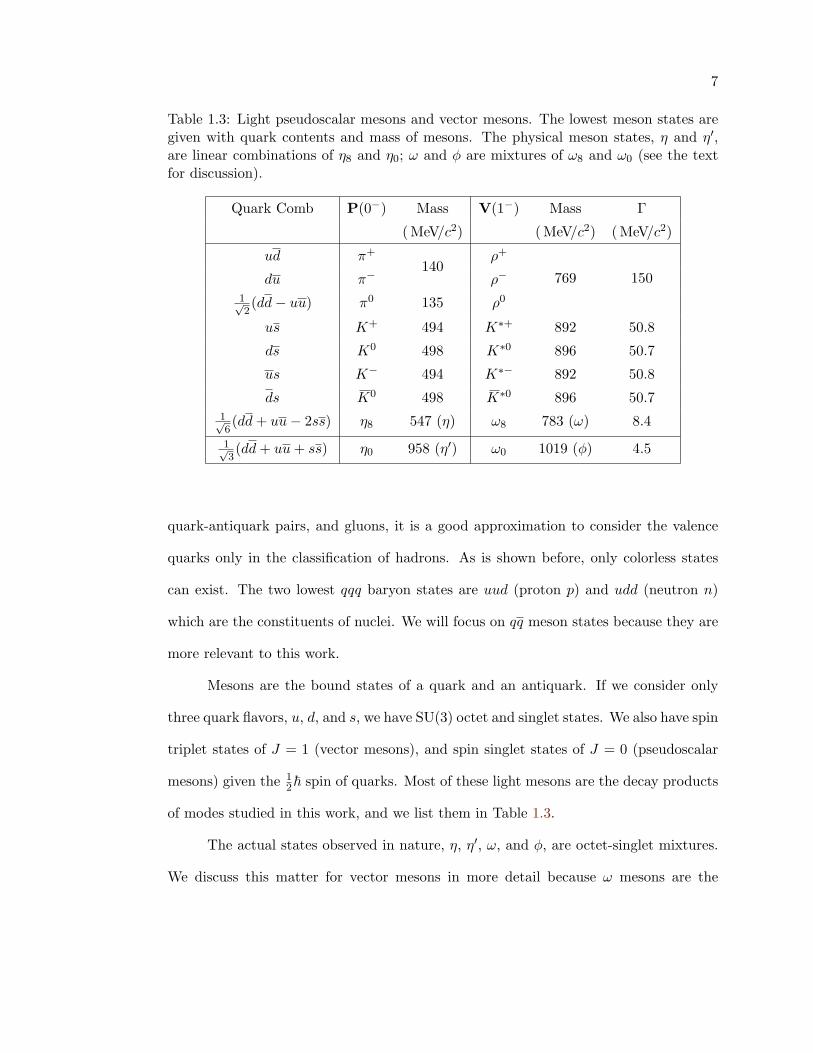
Table 1.3: Light pseudoscalar mesons and vector mesons. The lowest meson states aregiven with quark contents and mass of mesons. The physical meson states, η and η′,are linear combinations of η8 and η0; ω and φ are mixtures of ω8 and ω0 (see the textfor discussion).

Quark Comb P(0−) Mass V(1−) Mass Γ

( MeV/c2) ( MeV/c2) (MeV/c2)

ud π+ ρ+

du π−140

ρ−

1√2(dd− uu) π0 135 ρ0

769 150

us K+ 494 K∗+ 892 50.8

ds K0 498 K∗0 896 50.7

us K− 494 K∗− 892 50.8

ds K0 498 K∗0 896 50.71√6(dd+ uu− 2ss) η8 547 (η) ω8 783 (ω) 8.4

1√3(dd+ uu+ ss) η0 958 (η′) ω0 1019 (φ) 4.5

quark-antiquark pairs, and gluons, it is a good approximation to consider the valence

quarks only in the classification of hadrons. As is shown before, only colorless states

can exist. The two lowest qqq baryon states are uud (proton p) and udd (neutron n)

which are the constituents of nuclei. We will focus on qq meson states because they are

more relevant to this work.

Mesons are the bound states of a quark and an antiquark. If we consider only

three quark flavors, u, d, and s, we have SU(3) octet and singlet states. We also have spin

triplet states of J = 1 (vector mesons), and spin singlet states of J = 0 (pseudoscalar

mesons) given the 12~ spin of quarks. Most of these light mesons are the decay products

of modes studied in this work, and we list them in Table 1.3.

The actual states observed in nature, η, η′, ω, and φ, are octet-singlet mixtures.

We discuss this matter for vector mesons in more detail because ω mesons are the

8

subject of this work. We can write the mixing as:

φ = ω0 sin θ − ω8 cos θ ,

ω = ω8 sin θ + ω0 cos θ , (1.3)

where φ, ω denote the physical vector mesons, and ω0, ω8, defined as

ω0 =1√3(dd+ uu+ ss) ,

ω8 =1√6(dd+ uu− 2ss) , (1.4)

are the singlet and octet states, respectively. For the ‘ideal mixing’, sin θ = 1/√

3,

θ ' 35, (1.3) becomes

φ =1√3(ω0 −

√2ω8) ,

ω =1√3(ω8 +

√2ω0) , (1.5)

and with (1.4) we have

φ = ss ,

ω =1√2(uu+ dd) , (1.6)

which means φ is composed of s quarks and ω of u and d. The fact that φ decays

dominantly to KK while phase-space factors favor 3π decay, gives support to the ss

composition of φ. Eq. (1.6) also suggests larger mass for φ and similar masses for ω

and ρ, which is true as in Table 1.3, and the calculation of mixing angle based on mass

formulas gives θ ' 40, which is very close to the ideal case.

Mesons with heavier quarks are listed in Table 1.4. The first observed charmonium

state is J/ψ (cc); one c quark and a light quark form D mesons (pseudoscalars) and D∗

mesons (vectors). The first observed bound state of much heavier b quarks is Υ (bb);

one b quark and a light quark form B mesons (pseudoscalars) and B∗ mesons (vectors).

9

Table 1.4: Heavy mesons with c, b quarks.

Quark Comb Pseudoscalar (JP = 0−) Vector (JP = 1−)

cd, cd, cu, cu D+, D−, D0, D0 D∗+, D∗−, D∗0, D∗0

cs, cs D+s , D−

s D∗+s , D∗−

s

cc ηc J/ψ

bu, bu, bd, bd B+, B−, B0, B0 B∗+, B∗−, B∗0, B∗0

bs, bs B0s , B0

s B∗0s , B∗0

s

bb ηb Υ

The t quark is so massive with Mt ' 174 GeV/c2 that no bound state can be formed

before it decays to a b quark and a real W boson.

For heavy quark QQ states, such as bb (Υ ), the first term of (1.2) dominates

at small r, and the momentum transfer q is much less than the quark mass, so they

have similar energy levels as positronium, and then can be classified similarly by their

principal (radial) quantum number n, together with the orbital angular momentum L,

and the total spin S.

The vector Υ (4S) resonance is very important because it is just above the BB

production threshold and decays into BB pairs, so the B Factory of SLAC is operating

on the Υ (4S) resonance in order to produce large number of BB events. We will have

detailed discussion on B physics and B Factory in section 1.6 and 2.2, respectively.

1.4 Decay of Resonance

Mesons are often referred to as resonances because they are usually short-lived

bound states with finite width. In the rest frame of a particle of mass M , the rate of

decay into n bodies is given by [12]

dΓ =(2π)4

2M|M|2dΦn(P ; p1, . . . , pn) , (1.7)

10

where M is the Lorentz-invariant matrix element between initial and final states, and

dΦn is an element of n-body phase space given by

dΦn(P ; p1, . . . , pn) = δ4(P −n∑

i=1

pi)n∏

i=1

d3pi

(2π)32Ei. (1.8)

We are particularly interested in 2-body decays because they are the decay modes

studied in this work and are relatively simple. The rate of two-body decay can be

written as

dΓ =1

32π2|M|2 |p|

M2dΩ , (1.9)

where p is the momentum of one of the final particles. There is no angular dependence

for P → P1P2 (P for spinless pseudoscalar meson) decays so the width of the decay is

Γ =|p|

8πM2|M|2 , (1.10)

by integrating over the full solid angle.

Decays involving particles with spin have complicated angular distributions. We

can generally express the angular dependence for decays P → X1X2, where X could be

P (pseudoscalar), V (vector), etc., both X1 and X2 decaying into spinless particles, in

terms of the spherical functions [10,13]

d3Γd cos θ1d cos θ2dφ

∝ |∑

|m|≤J1,J2

Am × YJ1,m(θ1, φ1)× YJ2,−m(θ2, φ2)|2 , (1.11)

where θ1 and θ2 are the helicity angles defined by the direction of the two-body Xi

decay axis in the Xi rest frame (or by the normal to the three-body decay plane in the

Xi rest frame) relative to the Xi momentum, φ = φ1 − φ2 the azimuthal angle between

the two decay planes (for the case with both X1 and X2 decaying into two particles; see

Figure 1.2 for the definition of φ with X1 → P1P2P3); Am is the decay amplitude, and

Ji is the angular momentum quantum number for Xi.

For P → P1V2 decays, J1 = 0 and J2 = 1, then

dΓ ∝ |A0 × Y1,0(θ2, φ)|2d cos θ2dφ

∝ cos2 θ2d cos θ2 , (1.12)

11

π+

−π

θ1

φ

π0

π

ω

+π

θ2ρ+

0

d

mn

c

Figure 1.2: Helicity frame for B+ → ωρ+. n is the normal to the ω decay plane (theellipse) which is the plane of the 3π’s in the ω rest frame; m is the flight direction of π+

from ρ+, measured in the ρ+ rest frame; θ1 is defined as the angle between n and theflight direction of ω (helicity axis), measured in the ω rest frame; θ2 is defined as theangle between m and the direction of ρ in the ρ rest frame; c(d) is the unit vector alongthe projection of n (m) orthogonal to the direction of ω (ρ+); the azimuthal angle φ isdefined as the angle between c and d.

which means the helicity cosine H ≡ cos θH of the vector meson has a quadratic distri-

bution.

In P → V1V2 modes, J1 = 1 and J2 = 1, there are three amplitudes Aλ, (λ =

0,±1); then

1Γ

d3Γd cos θ1d cos θ2dφ

=9

16π1

|A0|2 + |A+1|2 + |A−1|2(1.13)

×

12

sin2 θ1 sin2 θ2(|A+1|2 + |A−1|2

)+ 2 cos2 θ1 cos2 θ2|A0|2

+sin2 θ1 sin2 θ2[cos 2φ <e(A+1A

∗−1)− sin 2φ =m(A+1A

∗−1)

]−1

2sin 2θ1 sin 2θ2

[cosφ <e(A+1A

∗0 +A−1A

∗0)− sinφ =m(A+1A

∗0 −A−1A

∗0)

],

where we may integrate over the azimuthal angles (assuming azimuthal uniformity of

12

1θcos-1

-0.50

0.512

θcos

-1-0.5

00.5

102468

101214

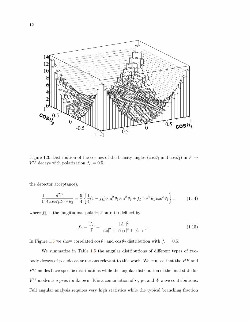
Figure 1.3: Distribution of the cosines of the helicity angles (cos θ1 and cos θ2) in P →V V decays with polarization fL = 0.5.

the detector acceptance),

1Γ

d2Γd cos θ1d cos θ2

=94

14(1− fL) sin2 θ1 sin2 θ2 + fL cos2 θ1 cos2 θ2

, (1.14)

where fL is the longitudinal polarization ratio defined by

fL =ΓL

Γ=

|A0|2

|A0|2 + |A+1|2 + |A−1|2. (1.15)

In Figure 1.3 we show correlated cos θ1 and cos θ2 distribution with fL = 0.5.

We summarize in Table 1.5 the angular distributions of different types of two-

body decays of pseudoscalar mesons relevant to this work. We can see that the PP and

PV modes have specific distributions while the angular distribution of the final state for

V V modes is a priori unknown. It is a combination of s-, p-, and d- wave contributions.

Full angular analysis requires very high statistics while the typical branching fraction

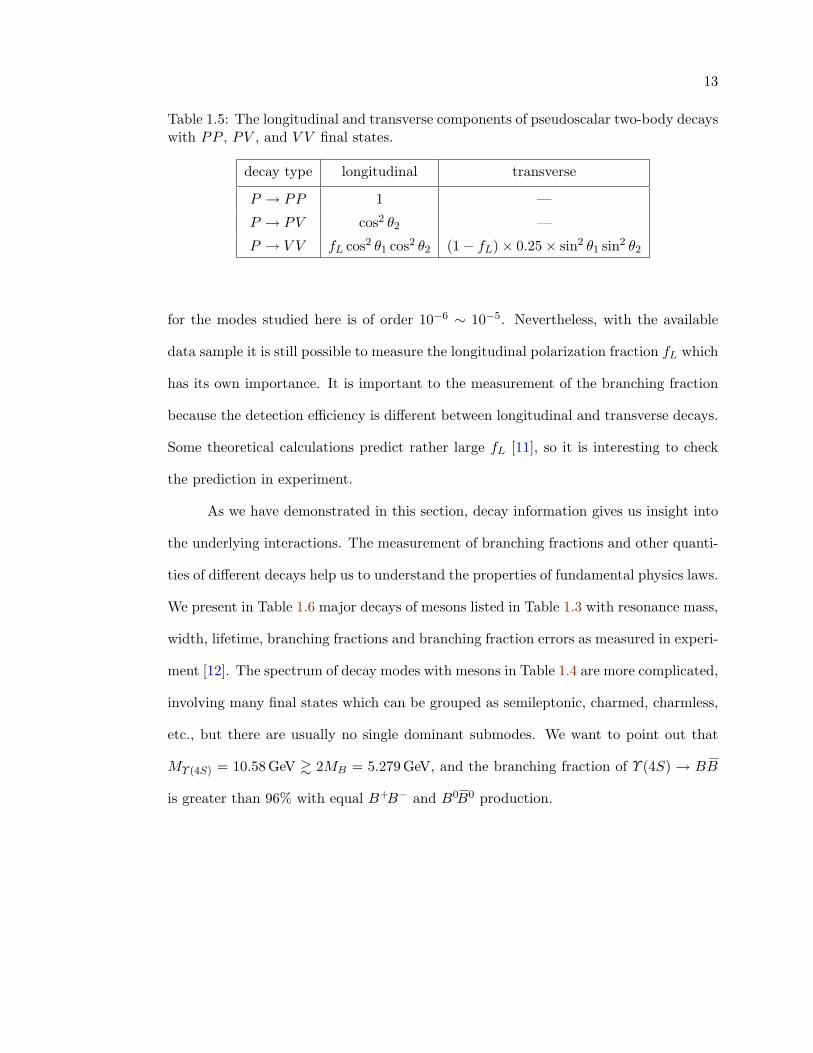
13

Table 1.5: The longitudinal and transverse components of pseudoscalar two-body decayswith PP , PV , and V V final states.

decay type longitudinal transverse

P → PP 1 —

P → PV cos2 θ2 —

P → V V fL cos2 θ1 cos2 θ2 (1− fL)× 0.25× sin2 θ1 sin2 θ2

for the modes studied here is of order 10−6 ∼ 10−5. Nevertheless, with the available

data sample it is still possible to measure the longitudinal polarization fraction fL which

has its own importance. It is important to the measurement of the branching fraction

because the detection efficiency is different between longitudinal and transverse decays.

Some theoretical calculations predict rather large fL [11], so it is interesting to check

the prediction in experiment.

As we have demonstrated in this section, decay information gives us insight into

the underlying interactions. The measurement of branching fractions and other quanti-

ties of different decays help us to understand the properties of fundamental physics laws.

We present in Table 1.6 major decays of mesons listed in Table 1.3 with resonance mass,

width, lifetime, branching fractions and branching fraction errors as measured in experi-

ment [12]. The spectrum of decay modes with mesons in Table 1.4 are more complicated,

involving many final states which can be grouped as semileptonic, charmed, charmless,

etc., but there are usually no single dominant submodes. We want to point out that

MΥ (4S) = 10.58 GeV & 2MB = 5.279 GeV, and the branching fraction of Υ (4S) → BB

is greater than 96% with equal B+B− and B0B0 production.

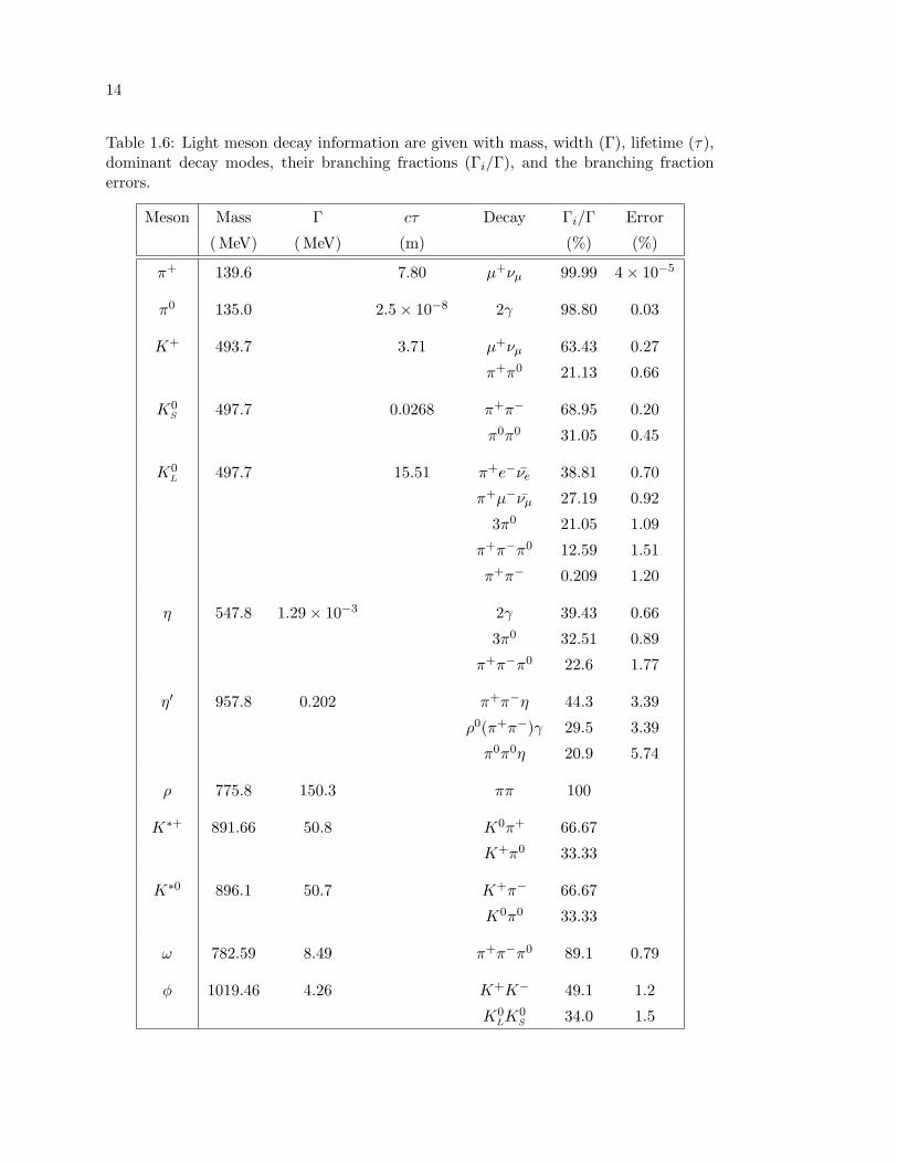
14

Table 1.6: Light meson decay information are given with mass, width (Γ), lifetime (τ),dominant decay modes, their branching fractions (Γi/Γ), and the branching fractionerrors.

Meson Mass Γ cτ Decay Γi/Γ Error

( MeV) (MeV) (m) (%) (%)

π+ 139.6 7.80 µ+νµ 99.99 4× 10−5

π0 135.0 2.5× 10−8 2γ 98.80 0.03

K+ 493.7 3.71 µ+νµ 63.43 0.27

π+π0 21.13 0.66

K0S 497.7 0.0268 π+π− 68.95 0.20

π0π0 31.05 0.45

K0L 497.7 15.51 π+e−νe 38.81 0.70

π+µ−νµ 27.19 0.92

3π0 21.05 1.09

π+π−π0 12.59 1.51

π+π− 0.209 1.20

η 547.8 1.29× 10−3 2γ 39.43 0.66

3π0 32.51 0.89

π+π−π0 22.6 1.77

η′ 957.8 0.202 π+π−η 44.3 3.39

ρ0(π+π−)γ 29.5 3.39

π0π0η 20.9 5.74

ρ 775.8 150.3 ππ 100

K∗+ 891.66 50.8 K0π+ 66.67

K+π0 33.33

K∗0 896.1 50.7 K+π− 66.67

K0π0 33.33

ω 782.59 8.49 π+π−π0 89.1 0.79

φ 1019.46 4.26 K+K− 49.1 1.2

K0LK

0S 34.0 1.5

15

1.5 Electroweak Interactions and CP Violation

The Standard Model is a gauge theory based on the SU(3)C × SU(2)L × U(1)Y

symmetry group, with three fermion generations, and CP violations arise from a single

phase in the quark mixing matrix [14].

The electromagnetic and weak interactions can be unified into a single electroweak

interaction through the SU(2)L×U(1)Y group: an SU(2)L group of ‘weak isospin’ I and

a U(1)Y group of ‘weak hypercharge’ Y . Three of the four massless mediating bosons,

Wµ = W(1)µ ,W

(2)µ ,W

(3)µ , are the components of an I = 1 isovector triplet, while the

fourth, Bµ, is an isosinglet. The minimal model also includes a single complex Higgs

scalar doublet φ ≡(φ+

φ0

), and with the so-called ‘spontaneous symmetry breaking’

process, due to the non-zero expectation value of the Higgs scalar field in the vacuum,

〈φ〉 = v 6= 0, three bosons, W+µ , W−

µ and Z0µ, acquire mass, and one, Aµ (the photon),

remains massless.

Each quark generation consists of three multiples,

QIL =

(uI

L

dIL

)= (3, 2)+1/6 , uI

R = (3, 1)+2/3 , dIR = (3, 1)−1/3 , (1.16)

where (3, 2)+1/6 denotes a triplet of SU(3)C , doublet of SU(2)L with hypercharge Y =

Q− I3 = +1/6, similarly for the other representations, uIL (uI

R) and dIL (dI

R) denote the

left-handed (right-handed) components of the up-type and down-type of quarks. The

interactions of quarks with the SU(2)L gauge bosons are described by

LW = −12gQI

Liγµτa1ijQ

ILjW

aµ , (1.17)

where g is the weak coupling constant, γµ operates in Lorentz space, τa operates in

SU(2)L space, and 1 is the unit matrix operating in generation (flavor) space. This unit

matrix is written explicitly to make the transformation to mass eigenbasis clearer. The

Lagrangian of quarks interacting with the Higgs fields can be written as

LY = −GijQILiφd

IRj − FijQI

LiφuIRj + h.c. , (1.18)

16

where G and F are general complex 3× 3 matrices. Their complex nature is the source

of CP violation in the Standard Model. We can expand the Higgs scalar field near its

vacuum state

φ0 =1√2

(0v

), (1.19)

so we have

φ =(φ+(x)φ0(x)

)→ 1√

2

(0

v +H0

), (1.20)

and the symmetry of the scalar field is broken, with which the two components of the

quark doublet become distinguishable, as are the three members of the Wµ triplet. The

charged current interaction in (1.17) then can be written as

LCC = −√

12guI

Liγµ1ijd

ILjW

+µ + h.c. . (1.21)

The expansion also endows quarks with mass terms when substituted in (1.18):

LM = −√

12vGijdI

LidIRj −

√12vFijuI

LiuIRj + h.c. , (1.22)

with the mass matrices being

Md = Gv/√

2, Mu = Fv/√

2 . (1.23)

In general, the quark weak interaction eigenstates in (1.16) are different from the mass

eigenstates, so the mass matrices in (1.23) are usually not diagonal. We can diagonalize

the mass matrices by introducing four unitary matrices such that

VdLMdV†dR = Mdiag

d , VuLMuV†uR = Mdiag

u , (1.24)

where Mdiagq are diagonal and real, while VqL and VqR are complex. In the mass eigen-

basis, the charged current interactions (1.21) becomes

LCC = −√

12guLiγ

µV ijdLjW+µ + h.c. . (1.25)

where u and d without superscript I (stands for weak Interaction) denote the mass

eigenstates of quarks, and the matrix V = VuLV†dL is the unitary mixing matrix for

three quark generations.

17

In general, there are nine parameters for the mixing matrix: three real angles

and six complex phases, however the number of phases in V can be reduced by a

transformation

V =⇒ V = PuV P∗d , (1.26)

where Pu and Pd are diagonal phase matrices. The five phase differences among the

elements of Pu and Pd can be chosen so that the transformation (1.26) eliminates five of

the six independent phases from V . Thus matrix V has one irreducible complex phase

and three real angles. The mixing matrix V is called the Cabibbo-Kobayashi-Maskawa

(CKM) matrix [15]

VCKM ≡

Vud Vus Vub

Vcd Vcs Vcb

Vtd Vts Vtb

, (1.27)

where each element Vqiqj represents the amplitude of flavor-changing weak interactions

between quarks qi and qj , and the phase is called the Kobayashi-Maskawa phase, δKM.

Three generations of quarks are necessary for the presence of the complex phase,

and therefore CP violation in the Standard Model. With two generations of quarks,

the Standard Model Lagrangian with a single Higgs field would remove all the complex

phases and the 2× 2 mixing matrix V is left with only one real parameter which is the

Cabibbo angle.

The fact that there is only one CP violating phase in the Standard Model im-

plies that all CP violating effects are very closely related. Therefore different physical

processes can be used to probe the same source of CP violation, and the redundancy

provides strict tests of the model.

18

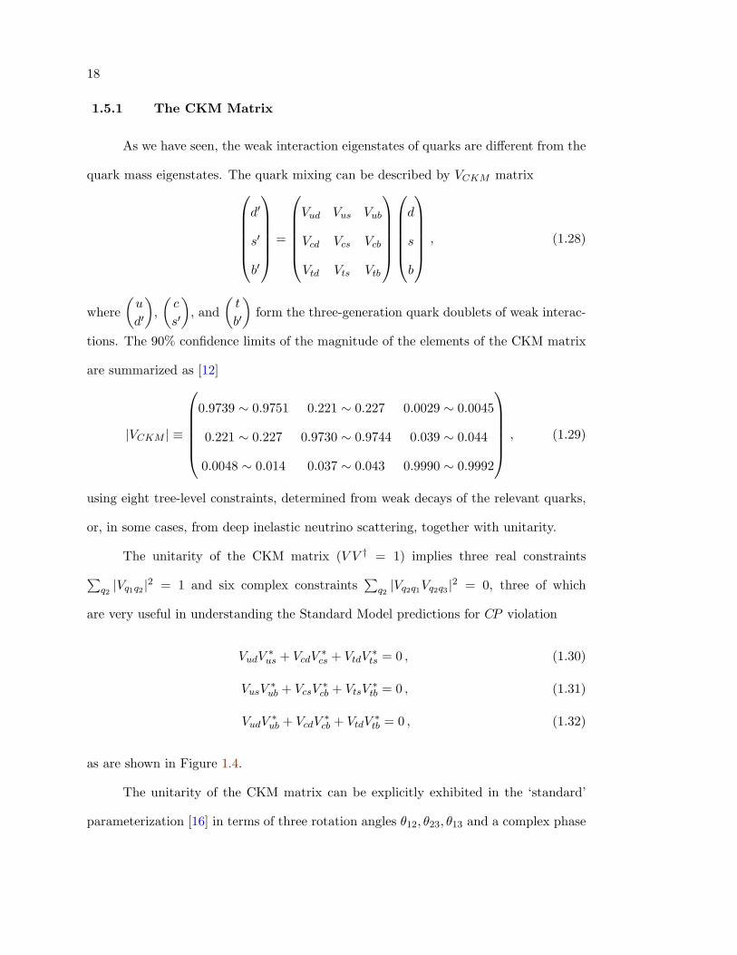
1.5.1 The CKM Matrix

As we have seen, the weak interaction eigenstates of quarks are different from the

quark mass eigenstates. The quark mixing can be described by VCKM matrixd′

s′

b′

=

Vud Vus Vub

Vcd Vcs Vcb

Vtd Vts Vtb

d

s

b

, (1.28)

where(u

d′

),(c

s′

), and

(t

b′

)form the three-generation quark doublets of weak interac-

tions. The 90% confidence limits of the magnitude of the elements of the CKM matrix

are summarized as [12]

|VCKM | ≡

0.9739 ∼ 0.9751 0.221 ∼ 0.227 0.0029 ∼ 0.0045

0.221 ∼ 0.227 0.9730 ∼ 0.9744 0.039 ∼ 0.044

0.0048 ∼ 0.014 0.037 ∼ 0.043 0.9990 ∼ 0.9992

, (1.29)

using eight tree-level constraints, determined from weak decays of the relevant quarks,

or, in some cases, from deep inelastic neutrino scattering, together with unitarity.

The unitarity of the CKM matrix (V V † = 1) implies three real constraints∑q2|Vq1q2 |2 = 1 and six complex constraints

∑q2|Vq2q1Vq2q3 |2 = 0, three of which

are very useful in understanding the Standard Model predictions for CP violation

VudV∗us + VcdV

∗cs + VtdV

∗ts = 0 , (1.30)

VusV∗ub + VcsV

∗cb + VtsV

∗tb = 0 , (1.31)

VudV∗ub + VcdV

∗cb + VtdV

∗tb = 0 , (1.32)

as are shown in Figure 1.4.

The unitarity of the CKM matrix can be explicitly exhibited in the ‘standard’

parameterization [16] in terms of three rotation angles θ12, θ23, θ13 and a complex phase

19

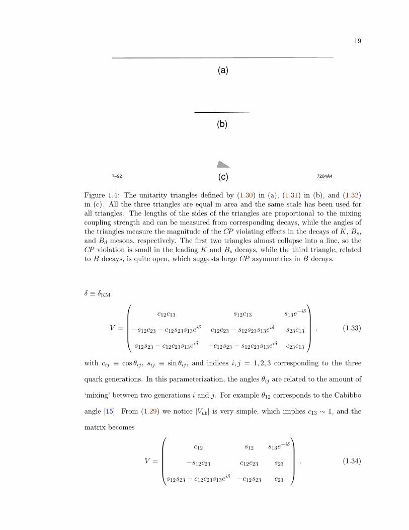
(c)

(b)

(a)

7204A47–92

Figure 1.4: The unitarity triangles defined by (1.30) in (a), (1.31) in (b), and (1.32)in (c). All the three triangles are equal in area and the same scale has been used forall triangles. The lengths of the sides of the triangles are proportional to the mixingcoupling strength and can be measured from corresponding decays, while the angles ofthe triangles measure the magnitude of the CP violating effects in the decays of K, Bs,and Bd mesons, respectively. The first two triangles almost collapse into a line, so theCP violation is small in the leading K and Bs decays, while the third triangle, relatedto B decays, is quite open, which suggests large CP asymmetries in B decays.

δ ≡ δKM

V =

c12c13 s12c13 s13e

−iδ

−s12c23 − c12s23s13eiδ c12c23 − s12s23s13e

iδ s23c13

s12s23 − c12c23s13eiδ −c12s23 − s12c23s13e

iδ c23c13

, (1.33)

with cij ≡ cos θij , sij ≡ sin θij , and indices i, j = 1, 2, 3 corresponding to the three

quark generations. In this parameterization, the angles θij are related to the amount of

‘mixing’ between two generations i and j. For example θ12 corresponds to the Cabibbo

angle [15]. From (1.29) we notice |Vub| is very simple, which implies c13 ∼ 1, and the

matrix becomes

V =

c12 s12 s13e

−iδ

−s12c23 c12c23 s23

s12s23 − c12c23s13eiδ −c12s23 c23

, (1.34)

20

where it is clear that the dominant phase terms are Vub and Vtd. It is convenient to

parameterize the CKM matrix in terms of four Wolfenstein parameters (A, λ, ρ, η) [17]

V =

1− λ2

2 λ Aλ3(ρ− iη)

−λ 1− λ2

2 Aλ2

Aλ3(1− ρ− iη) −Aλ2 1

+O(λ4) , (1.35)

with λ ≡ sin θC ' |Vus| ' 0.22, A ' 0.82, and η represents the CP violating phase

of the CKM matrix. The parameters of the standard parameterization (1.33) can be

related to the Wolfenstein parameters in (1.35) by

s12 ≡ λ, s23 ≡ Aλ2, s13e−iδ ≡ Aλ3(ρ− iη) . (1.36)

and we have

Vus = λ, Vcb = Aλ2, Vub = Aλ3(ρ− iη) , (1.37)

so we can write

Vtd = Aλ3(1− ρ− iη) , (1.38)

=mVcd = −A2λ5η , =mVts = −Aλ4η , (1.39)

with

ρ = ρ(1− λ2/2) , η = η(1− λ2/2) . (1.40)

We can rescale the Unitarity Triangle (1.32) by dividing all the three sides by

VcdV∗cb, such that two vertices of the rescaled Unitarity Triangle are fixed at (0,0) and

(1,0), while the third vertex is (ρ, η) in the Wolfenstein parameterizations (see Fig-

ure 1.5). The lengths of the two complex sides are

Rb ≡√ρ2 + η2 =

1− λ2/2λ

∣∣∣∣ Vub

|Vcb|

∣∣∣∣ , Rt ≡√

(1− ρ)2 + η2 =1λ

∣∣∣∣Vtd

Vcb

∣∣∣∣ , (1.41)

and the three angles are

α ≡ arg[−VtdV

∗tb

VudV∗ub

], β ≡ arg

[−VcdV

∗cb

VtdV∗tb

], γ ≡ arg

[−VudV

∗ub

VcdV∗cb

]≡ π−α−β , (1.42)

21

VudVub*

VtdVtb*

V Vcb*

cd

α

γ

β

a)

VudVub*

|VcdVcb* |

VtdVtb*

|VcdVcb* |

b)0

0

η

ρ

γ

1

β

α

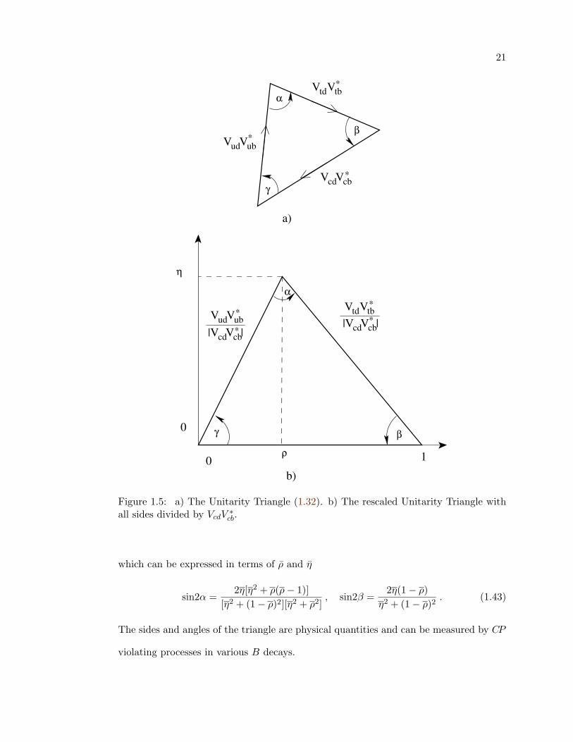
Figure 1.5: a) The Unitarity Triangle (1.32). b) The rescaled Unitarity Triangle withall sides divided by VcdV

∗cb.

which can be expressed in terms of ρ and η

sin2α =2η[η2 + ρ(ρ− 1)]

[η2 + (1− ρ)2][η2 + ρ2], sin2β =

2η(1− ρ)η2 + (1− ρ)2

. (1.43)

The sides and angles of the triangle are physical quantities and can be measured by CP

violating processes in various B decays.

22

1.5.2 CP Violation in B Decays

Three possible CP violation effects in the B decays are classified as

(1) “direct” CP violation in decay,

(2) “indirect” CP violation in mixing,∗

(3) CP violation in the interference between decays with and without mixing.

Direct CP violation in decay occurs when the amplitude for a decay and its CP conjugate

process have different magnitudes, which could happen in both charged and neutral

decays; indirect CP violation in mixing occurs when the two neutral mass eigenstates

are not CP eigenstates; CP violation in the interference between mixing and decay

occurs when the amplitude for a decay and its CP conjugate process have different

phases, which happens to decays with final states common to B0 and B0.

1.5.2.1 CP Violation in Decay

Direct CP violation is defined as the asymmetry of b and b decay rates

ACP =Γ(B → f)− Γ(B → f)Γ(B → f) + Γ(B → f)

, (1.44)

which is measurable for charged B decays because it is the only process that can give

CP violating effects for charged decays, and then it is also called charge asymmetry,

Ach =Γ(B− → f)− Γ(B+ → f)Γ(B− → f) + Γ(B+ → f)

, (1.45)

Though direct CP violation can also occur for neutral B decays, it competes with the

other two types of CP violating effects. For any final state f , each contribution to

the total decay amplitude Af has three parts: its magnitude Ai, its weak-phase term

eiφi , and its strong-phase term eiδi . The weak phases occur only in the CKM matrix

∗ See Sec. 1.5.2.2 for the meaning of mixing here

23

and have opposite signs for Af and Af , while the strong phases do not violate CP and

appear with the same signs for both Af and Af . So the total amplitude A(B → f) and

A(B → f) are:

Af =∑

i

Aiei(δi+φi) , Af =

∑i

Aiei(δi−φi) , (1.46)

where we omit the overall phase difference between Af and Af . Then the convention-

independent quantity is ∣∣∣∣Af

Af

∣∣∣∣ =∣∣∣∣∑iAie

i(δi−φi)∑iAiei(δi+φi)

∣∣∣∣ . (1.47)

When CP is conserved, the weak phases φi are all equal, and thus |Af/Af | = 1; then∣∣∣∣Af

Af

∣∣∣∣ 6= 1 =⇒ CP violation. (1.48)

The difference between the magnitudes |A| and |A| can be written as

|A|2 − |A|2 = −2∑i,j

AiAj sin(φi − φj) sin(δi − δj) , (1.49)

and we can see the CP violating effects arise from the interference among different phase

terms of the contributions to the total amplitude. ACP (1.44) can be expressed in terms

of the decay amplitude

ACP =1− |A/A|2

1 + |A/A|2. (1.50)

The only direct CP violation effect observed was in the K system [18, 19] before

the advent of PEP-II and KEKB.† Substantial direct CP violation in B decays can

arise from the interference of penguin (P ) and tree (T ) diagrams (see Sec. 1.6) [25]. In

the limit of T P , we have:

ACP ' 2∣∣∣∣TP

∣∣∣∣ sin∆φ sin∆δ , (1.51)

so sizable effects of ∼ 0.1 could be expected if ∆φ and ∆δ are not too small. How-

ever, calculation of such asymmetries is complicated by the presence of magnitude and

† The direct CP violation evidence in B decays is from B0 → K+π− by BABAR [20, 21], and fromB0 → π+π− by Belle [22].

24

strong phases involving long distance strong interactions and cannot be done from first

principles. The calculations generally contain two parts: First, the operator product

expansion and QCD perturbation theory are used to write any underlying quark process

as a sum of local quark operators with well-determined coefficients; second, the matrix

elements of the operators between the initial and final hadron states must be calculated.

We will discuss these theoretical approaches further in section 1.6 because of their im-

portance in understanding the rare B decays. Calculations based on effective theory and

factorization predict asymmetries in rare B meson decays of about ±10% [26]. These

expectations could be enhanced by larger phases due to FSI, for example, or due to new

physics beyond the Standard Model.

1.5.2.2 CP Violation in Mixing

In the neutral B system, the Hamiltonian eigenstates with definite mass and

lifetime are not the flavor eigenstates, namely, B0 = bd and B0 = bd. The flavor

eigenstates have definite quark content and are useful to understand particle production

and decay. Once B0 or B0 mesons are produced, they are mixing together through a

box diagram with two W exchange (Figure 1.6). This process is usually called B0– B0

oscillation and was first observed by the ARGUS [23] and UA1 [24] collaborations.

The Hamiltonian H describing the neutral B meson system can be written as

H = M − i

2Γ , (1.52)

where M and Γ are 2× 2 Hermitian matricesH11 H12

H21 H22

=

M M12

M∗12 M

− i

2

Γ Γ12

Γ∗12 Γ

, (1.53)

where H11 = H22. The off-diagonal terms, M12 and Γ12 are due to second order B0–

B0 transition via on-shell intermediate states, and are particularly important in the

discussion of CP violation. The Schrodinger equation of a linear combination of the

25

B0 B0

u, c, t

W− W+

u, c, t

d

b

b

d

Figure 1.6: Feynman diagram describing B0 – B0 mixing.

neutral B flavor eigenstates,

a|B0〉+ b|B0〉 , (1.54)

can then be written as

id

dt

(a

b

)= H

(a

b

)= (M − i

2Γ)

(a

b

). (1.55)

The two mass eigenstates, BL (for light B) and BH (for heavy B) can be expressed as

|BL〉 = p|B0〉+ q|B0〉 , (1.56)

|BH〉 = p|B0〉 − q|B0〉 , (1.57)

where the complex coefficients p and q satisfy

|q|2 + |p|2 = 1 , (1.58)

and we can then express B0 and B0 in terms of BL and BH

|B0〉 =12p

(|BL〉+ |BH〉) , (1.59)

|B0〉 =12q

(|BL〉 − |BH〉) . (1.60)

The mass and width of the light (heavy) B are ML (MH) and ΓL (ΓH), respectively, so

26

the two mass eigenstates evolve in time as

|BL(t)〉 = e−iMLte−ΓLt|BL(t = 0)〉 , (1.61)

|BH(t)〉 = e−iMH te−ΓH t|BH(t = 0)〉 , (1.62)

and we define the mass difference ∆md and width difference ∆Γ as

∆md ≡MH −ML , ∆Γ ≡ ΓH − ΓL , (1.63)

then we get by solving the Schrodinger equation of the system (1.55)

(∆md)2 −14(∆Γ)2 = 4(|M12|2 −

14|Γ12|2) , (1.64)

∆md∆Γ = 4 <e(M12Γ∗12), (1.65)

q

p= −

∆md − i2∆Γ

2(M12 − i2Γ12)

= −2(M∗

12 − i2Γ∗12)

∆md − i2∆Γ

, (1.66)

The magnitude of (1.66) is independent of phase conventions and is physically

meaningful ∣∣∣∣qp∣∣∣∣2 =

∣∣∣∣M∗12 − i

2Γ∗12M12 − i

2Γ12

∣∣∣∣ . (1.67)

When CP is conserved, the mass eigenstates are CP eigenstates, and the relative phase

between M12 and Γ12 vanishes, which gives |q/p| = 1, and then (1.67) implies∣∣∣∣qp∣∣∣∣ 6= 1 =⇒ CP violation. (1.68)

This type of CP violation is called CP violation in mixing and is often referred to

as “indirect” CP violation. It has been observed in the neutral K system through

semileptonic decays. For neutral B system, the indirect CP violating effect could be

measured through time-dependent asymmetries in semileptonic decays,

asl =Γ(B0(t) → l+µX)− Γ(B0(t) → l−µX)Γ(B0(t) → l+µX) + Γ(B0(t) → l−µX)

, (1.69)

which can be expressed in terms of |q/p|,

asl =1− |q/p|4

1 + |q/p|4. (1.70)

27

The expected CP violation in mixing of neutral B decays is small, O(10−2), since q/p is

close to unity, and it is also difficult to relate such asymmetries to the CKM parameters

because of theoretical uncertainties in the calculation of Γ12 and M12.

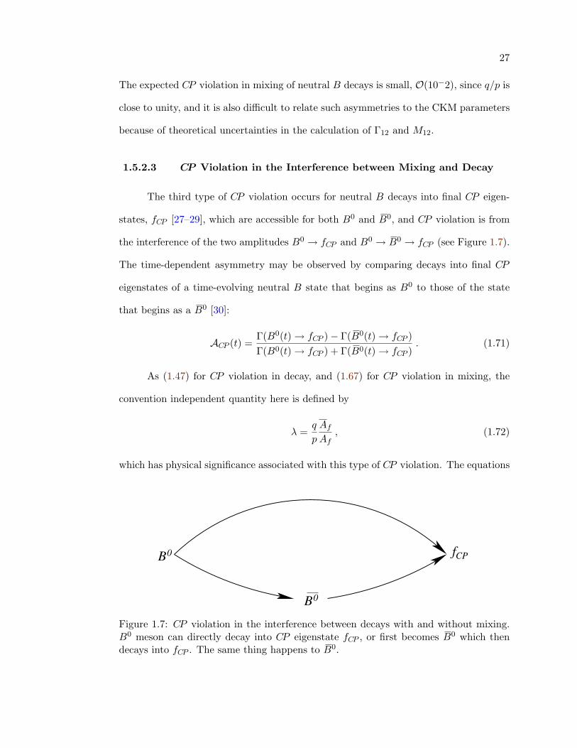
1.5.2.3 CP Violation in the Interference between Mixing and Decay

The third type of CP violation occurs for neutral B decays into final CP eigen-

states, fCP [27–29], which are accessible for both B0 and B0, and CP violation is from

the interference of the two amplitudes B0 → fCP and B0 → B0 → fCP (see Figure 1.7).

The time-dependent asymmetry may be observed by comparing decays into final CP

eigenstates of a time-evolving neutral B state that begins as B0 to those of the state

that begins as a B0 [30]:

ACP (t) =Γ(B0(t) → fCP )− Γ(B0(t) → fCP )Γ(B0(t) → fCP ) + Γ(B0(t) → fCP )

. (1.71)

As (1.47) for CP violation in decay, and (1.67) for CP violation in mixing, the

convention independent quantity here is defined by

λ =q

p

Af

Af, (1.72)

which has physical significance associated with this type of CP violation. The equations

fCP B

B

0

0

Figure 1.7: CP violation in the interference between decays with and without mixing.B0 meson can directly decay into CP eigenstate fCP , or first becomes B0 which thendecays into fCP . The same thing happens to B0.

28

(1.64), (1.65), and (1.66) can be simplified into

∆md = 2|M12| , ∆Γ = 2 <e(M12Γ∗12)/|M12| , (1.73)

q/p = −|M12|/M12 , (1.74)

considering that ∆Γ Γ [31]

∆Γ/Γ = O(10−2) , (1.75)

and ∆md has been measured [12],

xd ≡ ∆md/Γ = 0.771± 0.012 , (1.76)

and we can get

∆Γ ∆md . (1.77)

We are interested in the time evolution of neutral B state, |B0phys〉, which is pure B0

when created at time t = 0, and similarly for |B0phys〉, pure B0 at t = 0. From (1.59)

and (1.60) we get

|B0phys(t)〉 = g+(t)|B0〉+ (q/p)g−(t)|B0〉 , (1.78)

|B0phys(t)〉 = (p/q)g−(t)|B0〉+ g+(t)|B0〉 , (1.79)

where

g+(t) = e−iMte−Γt/2 cos(∆md t/2) , (1.80)

g−(t) = e−iMte−Γt/2i sin(∆md t/2) , (1.81)

and M = 12(MH +ML).

In the BABAR experiment, B0B0 pairs from Υ (4S) are produced in a coherent

L = 1 state, which means that while each of the two particles evolves in time as described

above, there is exactly one B0 and one B0 present, at any given time, before one of them

decays. Being such, we can ‘tag’ the flavor of B decaying into final CP eigenstate, fCP ,

29

using the other B, Btag, which decays into a tagging mode, that is a mode identifying

its b-flavor, at time ttag, then we know at time ttag, the flavor of the B to fCP is opposite

to Btag. The time-dependent rate for tagging B0 to decay at t = ttag and B0 to decay

to fCP at t = tfCPis given by

R(ttag, tfCP) = Ce−Γ(ttag+tfCP

)|Atag|2|AfCP|21 + |λfCP

|2

+cos[∆md(tfCP− ttag)](1− |λfCP

|2)− 2 sin[∆md(tfCP− ttag)] =m(λfCP

) , (1.82)

where C is an overall normalization factor, Atag is the amplitude for B0 to decay to

tagging mode, AfCPis the amplitude for B0 to decay to fCP , and

λfCP≡ q

p

AfCP

AfCP

= ηfCP

q

p

AfCP

AfCP

, (1.83)

where ηfCPis the CP eigenvalue of the state fCP and

AfCP= ηfCP

AfCP. (1.84)

A similar equation to (1.82), with reversed signs for both cosine and sine terms, applies

for the case where B0 is the tagging B identifying the second B as B0 at time ttag.

Then the time-dependent CP asymmetry (1.71) is

ACP (t) =1− |λfCP

|2

1 + |λfCP|2

cos ∆mdt−2 =mλfCP

1 + |λfCP|2

sin∆mdt , (1.85)

where t = tfCP− ttag.

If CP is conserved, |q/p| = 1, |AfCP/AfCP

| = 1, and furthermore, λfCP= ±1, so,

as we can see from (1.85)

λfCP6= ±1 =⇒ CP violation. (1.86)

Any CP violation from (1.48) or (1.68), leads to (1.86), even if there is no CP violation

from the first two types, i.e., |q/p| = 1 and |A/A| = 1, it is still possible to have CP

violating effect, if

|λfCP| = 1, =mλfCP

6= 0 . (1.87)

30

In such case, (1.85) can be reduced to

ACP (t) = − =mλfCPsin(∆mdt) . (1.88)

We can define

Af = Aei(φW +δ) , (1.89)

Af = ηfCPAei(−φW +δ) , (1.90)

q/p = e−2iφM , (1.91)

and then

λfCP= ηfCP

e−2i(φW−φM ), , (1.92)

where we can further write (1.88) as

ACP (t) = ηfCPsin(2φW − 2φM ) sin(∆mdt) . (1.93)

Measurements of ACP (t) from these ‘clean’ modes allow us to extract the angles of Uni-

tarity Triangle. For example, in decay B0 → ψK0S , 2φW −2φM = 2β, allows to measure

sin2β; in decay B0 → π+π−, 2φW − 2φM = 2α, allows to measure sin2α, though the

“penguin pollution” (see Sec 1.6 below) makes the measurement more challenging. The

richness of B decays provides many ways to determine the Unitarity Triangle parameters

and the consistency of the results offers an important test of the Standard Model.

1.6 Hadronic B Decays

1.6.1 Decay Diagrams

The flavor-changing weak decays of b quark are mediated by W± boson as in

the Lagrangian (1.25) describing the charged current interactions. Though there is no

flavor-changing neutral current in the Standard Model, an ‘effective’ neutral current,

introduced by loop, or “penguin” [32], transition, can have contributions to most decay

channels [25]. The penguins are classified according to the roles of the quark in the loop,

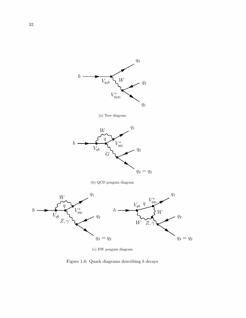
31

because diagrams with different intermediate quarks may have both different strong

phases and weak phases. The gluonic and electroweak penguins have the same phase

structure. However, the electroweak penguins are usually suppressed of an order of 10−1

relative to the corresponding gluonic penguins because of smaller coupling constants [33],

though they can be enhanced by a factor of M2t /M

2Z in certain cases. We show in

Figure 1.8 the quark diagrams for tree, penguin and electroweak penguin contributions.

The decay amplitude A(qqq′) for b→ qqq′ can be written as [10]

A(qqq′) = VtbV∗tq′P

tq′ + VcbV

∗cq′(Tccq′δqc + P c

q′) + VubV∗uq′(Tuuq′δqu + P u

q′) , (1.94)

where P and T denote contributions from tree-level and penguin diagrams, excluding

the CKM elements.

The quark-level amplitude, however, can not be used directly to calculate the

amplitude of B hadronic decays because of strong interactions between quarks in final

states. They are still useful to classify the types of decays. We are particularly fo-

cusing on rare charmless hadronic B decays of B → h1h2, where h1 and h2 are light

pseudoscalar (vector) mesons in the flavor U(3) nonet as in Table 1.3. These decays

involve the tree diagrams and/or penguin diagrams, with both gluonic and electroweak

penguin contributions [34]. The rare B decays with |∆S| = 1 involve a K or K∗ meson

in the final state and have Cabibbo suppressed tree-level b→ uus and dominant gluonic

penguin b→ sg∗ contributions, while decays with |∆S| = 0 are expected to have domi-

nant contributions from Cabibbo favored tree-level b→ uud diagram, and the penguin

process b→ dg∗ is suppressed by Vtd.

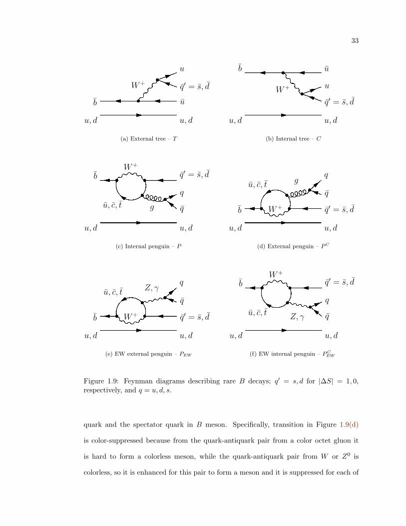
We show in Figure 1.9 the Feynman diagrams [35, 36]: (a) external tree – T , (b)

internal tree – C, (c) internal penguin – P , (d) external penguin – PC , (e) electroweak

external penguin – PEW , and (f) electroweak internal penguin – PCEW . In addition to

the CKM suppression or CKM enhancement of different contributions, there are other

rules to suppress a particular final state which is formed by the decay product of b

32

Wb

q1

q2

q3

Vq3b

V ∗

q2q1

(a) Tree diagram

G

W

b

q3 = q2

q2

q1

q

Vqb

V ∗

qq1

(b) QCD penguin diagram

Z, γ

W

b

q3 = q2

q2

q1

q

Vqb

V ∗

qq1

q

W

W

Z, γ

b

q3 = q2

q2

q1

Vqb

V ∗

qq1

(c) EW penguin diagram

Figure 1.8: Quark diagrams describing b decays

33

W+

u, d

b

u, d

u

q′ = s, d

u

(a) External tree – T

W+

u, d

b

u, d

q′ = s, d

u

u

(b) Internal tree – C

W+

u, c, t g

u, d

b

u, d

q

q

q′ = s, d

(c) Internal penguin – P

W+

u, c, tg

u, d

b

u, d

q′ = s, d

q

q

(d) External penguin – P C

W+

u, c, tZ, γ

u, d

b

u, d

q′ = s, d

q

q

(e) EW external penguin – PEW

W+

u, c, tZ, γ

u, d

b

u, d

q

q

q′ = s, d

(f) EW internal penguin – P CEW

Figure 1.9: Feynman diagrams describing rare B decays; q′ = s, d for |∆S| = 1, 0,respectively, and q = u, d, s.

quark and the spectator quark in B meson. Specifically, transition in Figure 1.9(d)

is color-suppressed because from the quark-antiquark pair from a color octet gluon it

is hard to form a colorless meson, while the quark-antiquark pair from W or Z0 is

colorless, so it is enhanced for this pair to form a meson and it is suppressed for each of

34

them to form a meson with other quarks. Thus, diagrams in Figure 1.9(b) and 1.9(f)

are color suppressed. As stated before, electroweak penguins are suppressed because of

small coupling constants relative to gluonic penguins. Other sources of suppression may

include delicate cancellations due to competition among different diagrams [34].

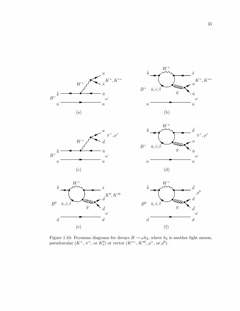
Particularly as the subject of this work, we will study decays B → h1h2, where

h1 is a vector meson, ω, and h2 is another light meson, pseudoscalar (K+, π+, or K0S)

or vector (K∗+, K∗0, ρ+, or ρ0). Because these charmless B decays involve couplings

with small CKM mixing matrix elements, several amplitudes potentially contribute with

similar strengths, as indicated in Figure 1.10. The B+ modes receive contributions from

external tree, color-suppressed tree, and penguin amplitudes, with the penguin strongly

favored by CKM couplings for B+ → ωK+, B+ → ωK∗+, and the external tree favored

for B+ → ωπ+, B+ → ωρ+. For the B0 modes there are no external tree contributions,

and again for B0 → ωK0, B0 → ωK∗0 the penguin is CKM-favored. For B0 → ωρ0

the color-suppressed trees cancel, leaving only a Cabibbo suppressed penguin, which

gives rather small expected branching fraction.

1.6.2 Low-Energy Effective Hamiltonians

Direct QCD calculations of hadronic decays give very limited information because

of non-perturbation of strong interaction at long distance. One of the most efficient tools

to do quantitative analysis of B decays is based on the low-energy effective Hamiltonian

[37], which is constructed using the operator product expansion (OPE) with transition

matrix elements of the form

〈f |Heff |i〉 ∝∑

k

〈f |Qk(µ)|i〉Ck(µ) , (1.95)

where µ denotes a renormalization scale, 〈f |Qk(µ)|i〉 are the nonperturbative hadronic

matrix elements describing the long-distance contributions to the decay amplitude,

Ck(µ) are the perturbatively calculable Wilson coefficient functions describing the short-

35

B+ ω

K+, K∗+

W+

u

b

u

u

s

u

B+

ω

K+, K∗+

W+

u, c, tg

u

b

u

u

u

s

(a) (b)

B+ ω

π+, ρ+

W+

u

b

u

u

d

u

B+

ω

π+, ρ+

W+

u, c, tg

u

b

u

u

u

d

(c) (d)

B0

ω

K0, K∗0

W+

u, c, tg

d

b

d

d

d

s

B0

ω

ρ0

W+

u, c, tg

d

b

d

d

d

d

(e) (f)

Figure 1.10: Feynman diagrams for decays B → ωh2, where h2 is another light meson,pseudoscalar (K+, π+, or K0

S) or vector (K∗+, K∗0, ρ+, or ρ0).

36

distance contributions.

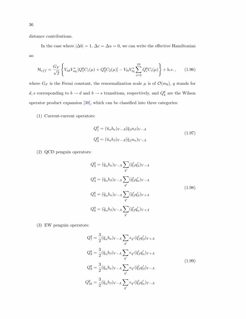
In the case where |∆b| = 1, ∆c = ∆u = 0, we can write the effective Hamiltonian

as:

Heff =GF√

2

VubV

∗uq [Qq

1C1(µ) +Qq2C2(µ)]− VtbV

∗tq

10∑i=3

QqiCi(µ)

+ h.c. , (1.96)

where GF is the Fermi constant, the renormalization scale µ is of O(mb), q stands for

d, s corresponding to b→ d and b→ s transitions, respectively, and Qqk are the Wilson

operator product expansion [38], which can be classified into three categories:

(1) Current-current operators:

Qq1 = (uαbα)V−A(qβuβ)V−A

Qq2 = (uαbβ)V−A(qβuα)V−A

(1.97)

(2) QCD penguin operators:

Qq3 = (qαbα)V−A

∑q′

(q′βq′β)V−A

Qq4 = (qαbβ)V−A

∑q′

(q′βq′α)V−A

Qq5 = (qαbα)V−A

∑q′

(q′βq′β)V +A

Qq6 = (qαbβ)V−A

∑q′

(q′βq′α)V +A

(1.98)

(3) EW penguin operators:

Qq7 =

32(qαbα)V−A

∑q′

eq′(q′βq′β)V +A

Qq8 =

32(qαbβ)V−A

∑q′

eq′(q′βq′α)V +A

Qq9 =

32(qαbα)V−A

∑q′

eq′(q′βq′β)V−A

Qq10 =

32(qαbβ)V−A

∑q′

eq′(q′βq′α)V−A

(1.99)

37

where (q1q2)V±A ≡ q1γµ(1 ± γ5)q2, α and β are SU(3) color indices, q′ runs over the

quark flavors to the scale µ = O(mb), i.e., q′ ∈ u, d, c, s, b, and eq′ is the electrical

charge of q′.

Since the hadronic matrix elements 〈h1h2|Qqk|B〉 are too complicated to be cal-

culated in lattice-QCD methods, the approach employed here is based on factoriza-

tion [26, 34, 39–41], where with the factorization Ansatz, the matrix element can be

factorized into the product of two factors 〈h1|J1|B〉〈h2|J2|0〉, where J1 and J2 are cur-

rent operators determined by form factors and decay constants, which are theoretically

more tractable and can be calculated in well-defined theoretical frameworks, such as

lattice-QCD [42], QCD sum rules [43], and potential model [44]. One can then make

quantitative predictions, for example, to the decay rates of B → h1h2, in this framework,

with guidance from experiments as the input parameters. The theoretical predictions

have many uncertainties: CKM matrix elements, quark masses, form factors, etc., so

they are usually given as ranges. We summarize predictions [45–50] and previous

measurements [51–53] for modes studied here in Table 1.7.

The factorization procedure is justified by the phenomenon of color-transparency

[54], that a pair of energetic quarks in a color-singlet state effectively decouples from

soft gluons. For the decays B → h1h2, with Eh1,h2 ∼ MB/2, the energy of the quarks

leaving the interaction is large, so the (soft) final state interactions (FSI) due to gluon

exchange are small and factorization is a good approximation.

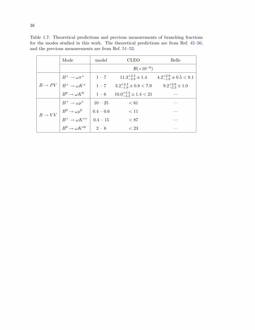
38

Table 1.7: Theoretical predictions and previous measurements of branching fractionsfor the modes studied in this work. The theoretical predictions are from Ref. 45–50,and the previous measurements are from Ref. 51–53.

Mode model CLEO Belle

B(×10−6)

B → PV

B+ → ωπ+ 1 – 7 11.3+3.3−2.9 ± 1.4 4.2+2.0

−1.8 ± 0.5 < 8.1

B+ → ωK+ 1 – 7 3.2+2.4−1.9 ± 0.8 < 7.9 9.2+2.6

−2.3 ± 1.0

B0 → ωK0 1 – 6 10.0+5.4−4.2 ± 1.4 < 21 —

B → V V

B+ → ωρ+ 10 – 25 < 61 —

B0 → ωρ0 0.4 – 0.6 < 11 —

B+ → ωK∗+ 0.4 – 15 < 87 —

B0 → ωK∗0 2 – 8 < 23 —

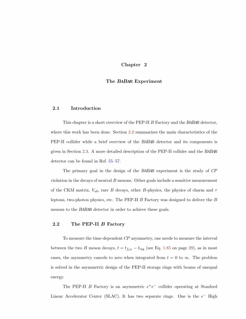
Chapter 2

The BABAR Experiment

2.1 Introduction

This chapter is a short overview of the PEP-II B Factory and the BABAR detector,

where this work has been done. Section 2.2 summarizes the main characteristics of the

PEP-II collider while a brief overview of the BABAR detector and its components is

given in Section 2.3. A more detailed description of the PEP-II collider and the BABAR

detector can be found in Ref. 55–57.

The primary goal in the design of the BABAR experiment is the study of CP

violation in the decays of neutral B mesons. Other goals include a sensitive measurement

of the CKM matrix, Vub, rare B decays, other B-physics, the physics of charm and τ

leptons, two-photon physics, etc. The PEP-II B Factory was designed to deliver the B

mesons to the BABAR detector in order to achieve these goals.

2.2 The PEP-II B Factory

To measure the time-dependent CP asymmetry, one needs to measure the interval

between the two B meson decays, t = tfCP− ttag (see Eq. 1.85 on page 29), as in most

cases, the asymmetry cancels to zero when integrated from t = 0 to ∞. The problem

is solved in the asymmetric design of the PEP-II storage rings with beams of unequal

energy.

The PEP-II B Factory is an asymmetric e+e− collider operating at Stanford

Linear Accelerator Center (SLAC). It has two separate rings. One is the e− High

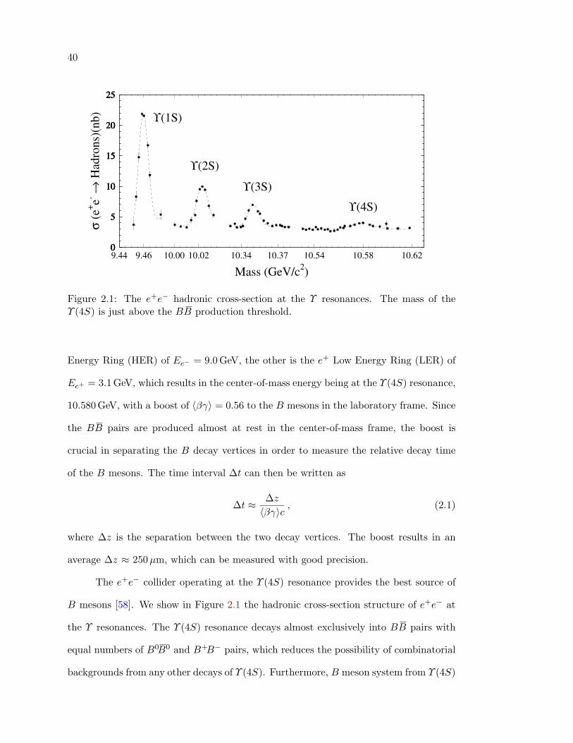
40

9.44 9.46

Mass (GeV/c2)

0

5

10

15

20

25σ

(e+ e- →

Had

rons

)(nb

) ϒ(1S)

10.00 10.020

5

10

15

20

25

ϒ(2S)

10.34 10.370

5

10

15

20

25

ϒ(3S)

10.54 10.58 10.620

5

10

15

20

25

ϒ(4S)

Figure 2.1: The e+e− hadronic cross-section at the Υ resonances. The mass of theΥ (4S) is just above the BB production threshold.

Energy Ring (HER) of Ee− = 9.0 GeV, the other is the e+ Low Energy Ring (LER) of

Ee+ = 3.1 GeV, which results in the center-of-mass energy being at the Υ (4S) resonance,

10.580GeV, with a boost of 〈βγ〉 = 0.56 to the B mesons in the laboratory frame. Since

the BB pairs are produced almost at rest in the center-of-mass frame, the boost is

crucial in separating the B decay vertices in order to measure the relative decay time

of the B mesons. The time interval ∆t can then be written as

∆t ≈ ∆z〈βγ〉c

, (2.1)

where ∆z is the separation between the two decay vertices. The boost results in an

average ∆z ≈ 250µm, which can be measured with good precision.

The e+e− collider operating at the Υ (4S) resonance provides the best source of

B mesons [58]. We show in Figure 2.1 the hadronic cross-section structure of e+e− at

the Υ resonances. The Υ (4S) resonance decays almost exclusively into BB pairs with

equal numbers of B0B0 and B+B− pairs, which reduces the possibility of combinatorial

backgrounds from any other decays of Υ (4S). Furthermore, B meson system from Υ (4S)

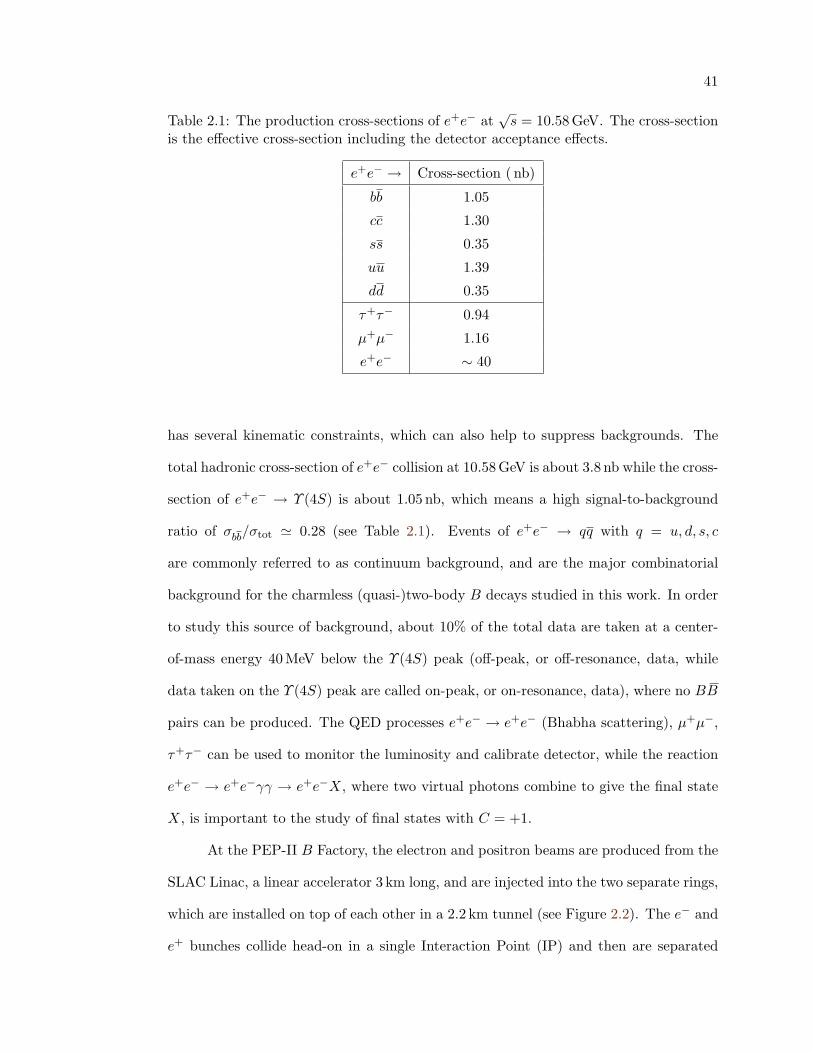
41

Table 2.1: The production cross-sections of e+e− at√s = 10.58 GeV. The cross-section

is the effective cross-section including the detector acceptance effects.

e+e− → Cross-section ( nb)

bb 1.05

cc 1.30

ss 0.35

uu 1.39

dd 0.35

τ+τ− 0.94

µ+µ− 1.16

e+e− ∼ 40

has several kinematic constraints, which can also help to suppress backgrounds. The

total hadronic cross-section of e+e− collision at 10.58 GeV is about 3.8 nb while the cross-

section of e+e− → Υ (4S) is about 1.05 nb, which means a high signal-to-background

ratio of σbb/σtot ' 0.28 (see Table 2.1). Events of e+e− → qq with q = u, d, s, c

are commonly referred to as continuum background, and are the major combinatorial

background for the charmless (quasi-)two-body B decays studied in this work. In order

to study this source of background, about 10% of the total data are taken at a center-

of-mass energy 40 MeV below the Υ (4S) peak (off-peak, or off-resonance, data, while

data taken on the Υ (4S) peak are called on-peak, or on-resonance, data), where no BB

pairs can be produced. The QED processes e+e− → e+e− (Bhabha scattering), µ+µ−,

τ+τ− can be used to monitor the luminosity and calibrate detector, while the reaction

e+e− → e+e−γγ → e+e−X, where two virtual photons combine to give the final state

X, is important to the study of final states with C = +1.

At the PEP-II B Factory, the electron and positron beams are produced from the

SLAC Linac, a linear accelerator 3 km long, and are injected into the two separate rings,

which are installed on top of each other in a 2.2 km tunnel (see Figure 2.2). The e− and

e+ bunches collide head-on in a single Interaction Point (IP) and then are separated

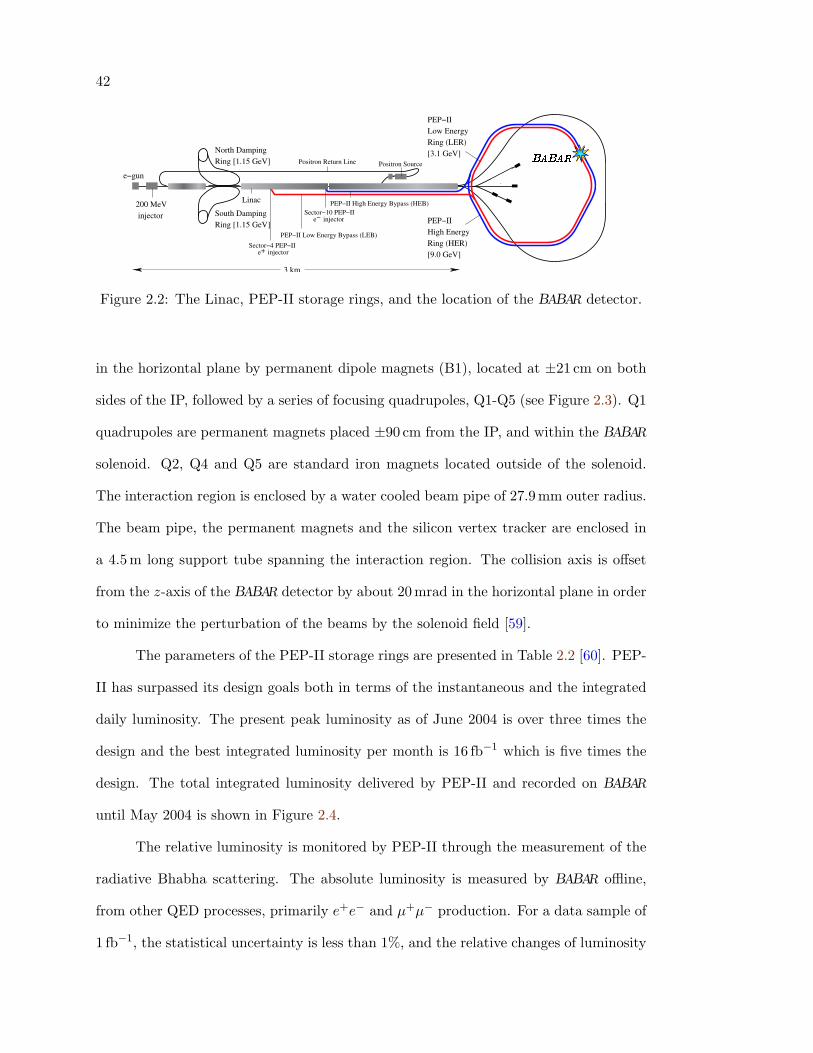
42

Ring [1.15 GeV]

Ring [1.15 GeV]South Damping

PEP−II

Ring (LER)[3.1 GeV]North Damping

PEP−II

[9.0 GeV]

High Energy

Low Energy

Ring (HER)

200 MeV Linac

Positron Return Line Positron Source

injector

3 km

PEP−II Low Energy Bypass (LEB)

PEP−II High Energy Bypass (HEB)

Sector−4 PEP−II

Sector−10 PEP−II−e injector

+e injector

e−gun

Figure 2.2: The Linac, PEP-II storage rings, and the location of the BABAR detector.

in the horizontal plane by permanent dipole magnets (B1), located at ±21 cm on both

sides of the IP, followed by a series of focusing quadrupoles, Q1-Q5 (see Figure 2.3). Q1

quadrupoles are permanent magnets placed ±90 cm from the IP, and within the BABAR

solenoid. Q2, Q4 and Q5 are standard iron magnets located outside of the solenoid.

The interaction region is enclosed by a water cooled beam pipe of 27.9mm outer radius.

The beam pipe, the permanent magnets and the silicon vertex tracker are enclosed in

a 4.5m long support tube spanning the interaction region. The collision axis is offset

from the z-axis of the BABAR detector by about 20 mrad in the horizontal plane in order

to minimize the perturbation of the beams by the solenoid field [59].

The parameters of the PEP-II storage rings are presented in Table 2.2 [60]. PEP-

II has surpassed its design goals both in terms of the instantaneous and the integrated

daily luminosity. The present peak luminosity as of June 2004 is over three times the

design and the best integrated luminosity per month is 16 fb−1 which is five times the

design. The total integrated luminosity delivered by PEP-II and recorded on BABAR

until May 2004 is shown in Figure 2.4.

The relative luminosity is monitored by PEP-II through the measurement of the

radiative Bhabha scattering. The absolute luminosity is measured by BABAR offline,

from other QED processes, primarily e+e− and µ+µ− production. For a data sample of

1 fb−1, the statistical uncertainty is less than 1%, and the relative changes of luminosity

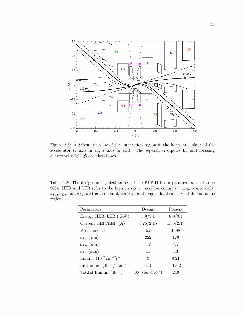
43

Q1

Q1

Q1

Q1

Q2Q4

Q4Q5

Q2

Q5

B1

B1 B1

B1

9 GeV

3.1 GeV

9 GeV

3.1 GeV

7.5–7.5 0–2.5–5.0 2.5 5.0–30

–20

–10

0

10

20

30

x (c

m)

z (m)

Figure 2.3: A Schematic view of the interaction region in the horizontal plane of theaccelerator (z axis in m, x axis in cm). The separation dipoles B1 and focusingquadrupoles Q1-Q5 are also shown.

Table 2.2: The design and typical values of the PEP-II beam parameters as of June2004. HER and LER refer to the high energy e− and low energy e+ ring, respectively.σLx, σLy, and σLz are the horizontal, vertical, and longitudinal rms size of the luminousregion.

Parameters Design Present

Energy HER/LER ( GeV) 9.0/3.1 9.0/3.1

Current HER/LER (A) 0.75/2.15 1.55/2.45

# of bunches 1658 1588

σLx (µm) 222 170

σLy (µm) 6.7 7.2

σLz (mm) 11 13

Lumin. (1033 cm−2s−1) 3 9.21

Int.Lumin. ( fb−1/mon.) 3.3 16.02

Tot.Int.Lumin. ( fb−1) 100 (for CPV ) 240

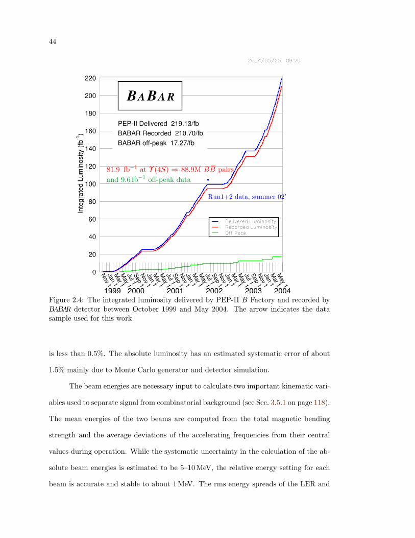
44

Nov 1

Jan 1

1999 M

ar 1 M

ay 1 Jul 1 Sep 1 N

ov 1 Jan 1

2000

Mar 1

May 1

Jul 1 Sep 1 N

ov 1 Jan 1

2001

Mar 1

May 1

Jul 1 Sep 1 N

ov 1 Jan 1

2002

Mar 1

May 1

Jul 1 Sep 1 N

ov 1 Jan 1

2003

Mar 1

May 1

2004

0

20

40

60

80

100

120

140

160

180

200

220In

tegr

ated

Lum

inos

ity (f

b-1)

BA BA R

PEP-II Delivered 219.13/fbBABAR Recorded 210.70/fbBABAR off-peak 17.27/fb

?

Run1+2 data, summer 02’

81.9 fb−1 at Υ (4S) ⇒ 88.9M BB pairsand 9.6 fb−1 off-peak data

Figure 2.4: The integrated luminosity delivered by PEP-II B Factory and recorded byBABAR detector between October 1999 and May 2004. The arrow indicates the datasample used for this work.

is less than 0.5%. The absolute luminosity has an estimated systematic error of about

1.5% mainly due to Monte Carlo generator and detector simulation.

The beam energies are necessary input to calculate two important kinematic vari-

ables used to separate signal from combinatorial background (see Sec. 3.5.1 on page 118).

The mean energies of the two beams are computed from the total magnetic bending

strength and the average deviations of the accelerating frequencies from their central

values during operation. While the systematic uncertainty in the calculation of the ab-

solute beam energies is estimated to be 5–10MeV, the relative energy setting for each

beam is accurate and stable to about 1 MeV. The rms energy spreads of the LER and

45

HER beams are 2.3MeV and 5.5MeV, respectively. BABAR also monitors the ratio of

BB events to lepton pairs and uses online fully reconstructed B events to ensure the

data are recorded close to the peak of Υ (4S) resonance. An absolute error of 1.1 MeV

to the c.m. energy is obtained for an integrated luminosity of 1 fb−1.

The parameters of the luminous region (see Table 2.2) are crucial for the time-

dependent analyses and their values are monitored continuously both online and offline

mainly using two-track events. The uncertainties in the average beam position are of the

order of a few µm in the transverse plane and 100µm along the collision axis. Run-by-

run variations of the beam position are comparable to these measurement uncertainties,

indicating the beams are stable over a period of a typical run.

The main sources of steady-state beam background are synchrotron radiation

in the vicinity of the interaction region; interactions between the beam particles and

the residual gas in either ring; and electromagnetic showers generated by beam-beam

collisions, in the order of increasing importance. The beam backgrounds can cause high

occupancy of the detector and may cause significant radiation damage to the detector

over time. Various methods are needed to monitor the backgrounds and protect the

detector against the radiation.

The layout of the interaction region and the synchrotron-radiation masks have

been designed such that most of the radiation is channeled to a distant dump, and the

residual background is relatively low without significant importance. The background

from beam-gas scattering can be improved significantly with time of operation because

of the scrubbing effects of the vacuum pipe by the synchrotron radiation. Neverthe-

less, beam-gas scattering remains the primary source of radiation damage in the SVT

and dominant source of background in all sub-detectors, except for the DIRC. The

background of electromagnetic showers generated by beam-beam collisions increases

proportionally with the instantaneous luminosity and is the dominant background in

the DIRC.

46

A system has been developed to monitor the instantaneous and integrated radi-

ation doses, and to either abort the beams or to halt or limit the rate of injection, if

conditions become critical, in order to protect the BABAR detector. In addition, DCH

and IFR currents, DIRC and IFR counting rates, are also monitored; abnormally high

rates signal critical conditions.

2.3 The BABAR Detector

The BABAR detector has been designed to operate optimally on the PEP-II B

Factory in order to achieve its physics goals.

For a large and uniform acceptance to the production on an asymmetric collider,

the BABAR detector needs to have a forward-backward asymmetric design along the

direction of the beam. The center of the BABAR detector is shifted by 0.37 m from the IP,

in the boost direction of the more energetic e− beam, as is shown in Figure 2.5. Other

asymmetric features include that the electromagnetic calorimeter only has a forward

end-cap; the read-out electronics of the drift chamber are placed at the backward end

of the detector.

The high luminosity needed for CP violation measurements and other rare B

decay studies requires unusual beam optics with machine components being very close

to the interaction region, and the BABAR detector needs to accommodate the machine

elements without much impact on its performance.

The vertexing system should have excellent vertex resolution along the z-axis

and in the transverse plane in order to measure the decay time distributions. Vertex

resolution also stresses the importance of minimizing multiple scattering.

High reconstruction efficiency and good momentum resolution for charged par-

ticles, together with reconstruction of the neutral particles, are important to fully re-

construct the final states of B decay, and to separate signal events from background.

The detector should be able to do tracking over a range of ∼ 60 MeV < pT <∼ 4 GeV,

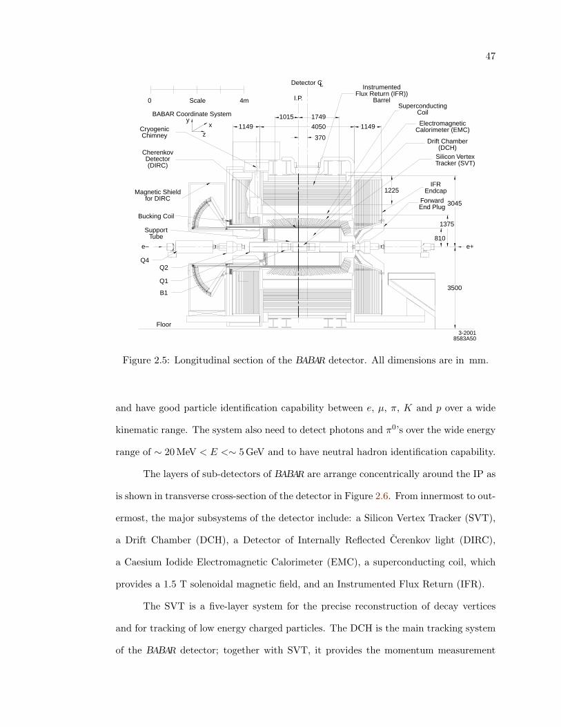
47

Scale

BABAR Coordinate System

0 4m

CryogenicChimney

Magnetic Shieldfor DIRC

Bucking Coil

CherenkovDetector(DIRC)

SupportTube

e– e+

Q4Q2

Q1

B1

Floor

yx

z1149 1149

InstrumentedFlux Return (IFR))

BarrelSuperconducting

Coil

ElectromagneticCalorimeter (EMC)

Drift Chamber(DCH)

Silicon VertexTracker (SVT)

IFREndcap

ForwardEnd Plug

1225

810

1375

3045

3500

3-20018583A50

1015 1749

4050

370

I.P.

Detector CL

Figure 2.5: Longitudinal section of the BABAR detector. All dimensions are in mm.

and have good particle identification capability between e, µ, π, K and p over a wide

kinematic range. The system also need to detect photons and π0’s over the wide energy

range of ∼ 20 MeV < E <∼ 5 GeV and to have neutral hadron identification capability.

The layers of sub-detectors of BABAR are arrange concentrically around the IP as

is shown in transverse cross-section of the detector in Figure 2.6. From innermost to out-

ermost, the major subsystems of the detector include: a Silicon Vertex Tracker (SVT),

a Drift Chamber (DCH), a Detector of Internally Reflected Cerenkov light (DIRC),

a Caesium Iodide Electromagnetic Calorimeter (EMC), a superconducting coil, which

provides a 1.5 T solenoidal magnetic field, and an Instrumented Flux Return (IFR).

The SVT is a five-layer system for the precise reconstruction of decay vertices

and for tracking of low energy charged particles. The DCH is the main tracking system

of the BABAR detector; together with SVT, it provides the momentum measurement

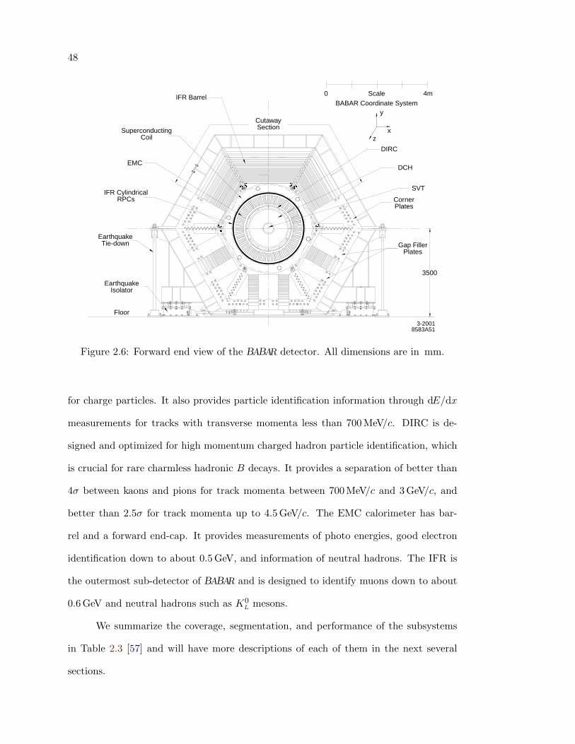
48

IFR Barrel

CutawaySection

ScaleBABAR Coordinate System

y

xz

DIRC

DCH

SVT

3500

CornerPlates

Gap FillerPlates

0 4m

SuperconductingCoil

EMC

IFR CylindricalRPCs

EarthquakeTie-down

EarthquakeIsolator

Floor

3-20018583A51

Figure 2.6: Forward end view of the BABAR detector. All dimensions are in mm.

for charge particles. It also provides particle identification information through dE/dx

measurements for tracks with transverse momenta less than 700 MeV/c. DIRC is de-

signed and optimized for high momentum charged hadron particle identification, which

is crucial for rare charmless hadronic B decays. It provides a separation of better than

4σ between kaons and pions for track momenta between 700 MeV/c and 3GeV/c, and

better than 2.5σ for track momenta up to 4.5 GeV/c. The EMC calorimeter has bar-

rel and a forward end-cap. It provides measurements of photo energies, good electron

identification down to about 0.5 GeV, and information of neutral hadrons. The IFR is

the outermost sub-detector of BABAR and is designed to identify muons down to about

0.6GeV and neutral hadrons such as K0L mesons.

We summarize the coverage, segmentation, and performance of the subsystems

in Table 2.3 [57] and will have more descriptions of each of them in the next several

sections.

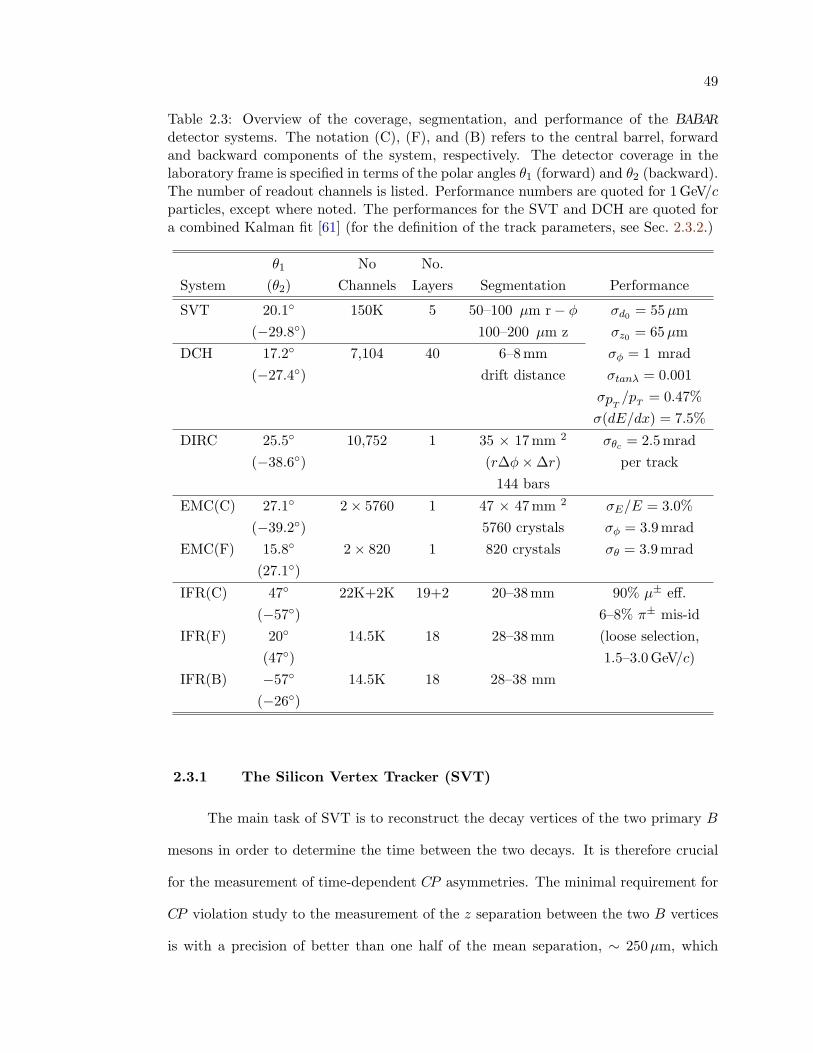
49

Table 2.3: Overview of the coverage, segmentation, and performance of the BABAR

detector systems. The notation (C), (F), and (B) refers to the central barrel, forwardand backward components of the system, respectively. The detector coverage in thelaboratory frame is specified in terms of the polar angles θ1 (forward) and θ2 (backward).The number of readout channels is listed. Performance numbers are quoted for 1 GeV/cparticles, except where noted. The performances for the SVT and DCH are quoted fora combined Kalman fit [61] (for the definition of the track parameters, see Sec. 2.3.2.)

θ1 No No.System (θ2) Channels Layers Segmentation Performance

SVT 20.1 150K 5 50–100 µm r− φ σd0 = 55µm(−29.8) 100–200 µm z σz0 = 65µm

DCH 17.2 7,104 40 6–8 mm σφ = 1 mrad(−27.4) drift distance σtanλ = 0.001

σpT/pT = 0.47%

σ(dE/dx) = 7.5%

DIRC 25.5 10,752 1 35 × 17 mm 2 σθc = 2.5 mrad(−38.6) (r∆φ×∆r) per track

144 bars

EMC(C) 27.1 2× 5760 1 47 × 47 mm 2 σE/E = 3.0%(−39.2) 5760 crystals σφ = 3.9 mrad

EMC(F) 15.8 2× 820 1 820 crystals σθ = 3.9 mrad(27.1)

IFR(C) 47 22K+2K 19+2 20–38 mm 90% µ± eff.(−57) 6–8% π± mis-id

IFR(F) 20 14.5K 18 28–38 mm (loose selection,(47) 1.5–3.0 GeV/c)

IFR(B) −57 14.5K 18 28–38 mm(−26)

2.3.1 The Silicon Vertex Tracker (SVT)

The main task of SVT is to reconstruct the decay vertices of the two primary B

mesons in order to determine the time between the two decays. It is therefore crucial

for the measurement of time-dependent CP asymmetries. The minimal requirement for

CP violation study to the measurement of the z separation between the two B vertices

is with a precision of better than one half of the mean separation, ∼ 250µm, which

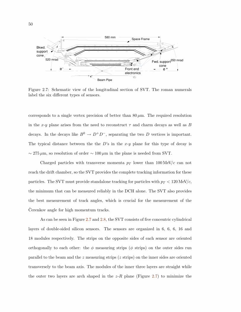
50

580 mm

350 mrad520 mrad

ee +-

Beam Pipe

Space Frame

Fwd. support cone

Bkwd. support cone

Front end electronics

Figure 2.7: Schematic view of the longitudinal section of SVT. The roman numeralslabel the six different types of sensors.

corresponds to a single vertex precision of better than 80µm. The required resolution

in the x-y plane arises from the need to reconstruct τ and charm decays as well as B

decays. In the decays like B0 → D+D−, separating the two D vertices is important.

The typical distance between the the D’s in the x-y plane for this type of decay is

∼ 275µm, so resolution of order ∼ 100µm in the plane is needed from SVT.

Charged particles with transverse momenta pT lower than 100 MeV/c can not

reach the drift chamber, so the SVT provides the complete tracking information for these

particles. The SVT must provide standalone tracking for particles with pT < 120 MeV/c,

the minimum that can be measured reliably in the DCH alone. The SVT also provides

the best measurement of track angles, which is crucial for the measurement of the

Cerenkov angle for high momentum tracks.

As can be seen in Figure 2.7 and 2.8, the SVT consists of five concentric cylindrical

layers of double-sided silicon sensors. The sensors are organized in 6, 6, 6, 16 and

18 modules respectively. The strips on the opposite sides of each sensor are oriented

orthogonally to each other: the φ measuring strips (φ strips) on the outer sides run

parallel to the beam and the z measuring strips (z strips) on the inner sides are oriented

transversely to the beam axis. The modules of the inner three layers are straight while

the outer two layers are arch shaped in the z-R plane (Figure 2.7) to minimize the

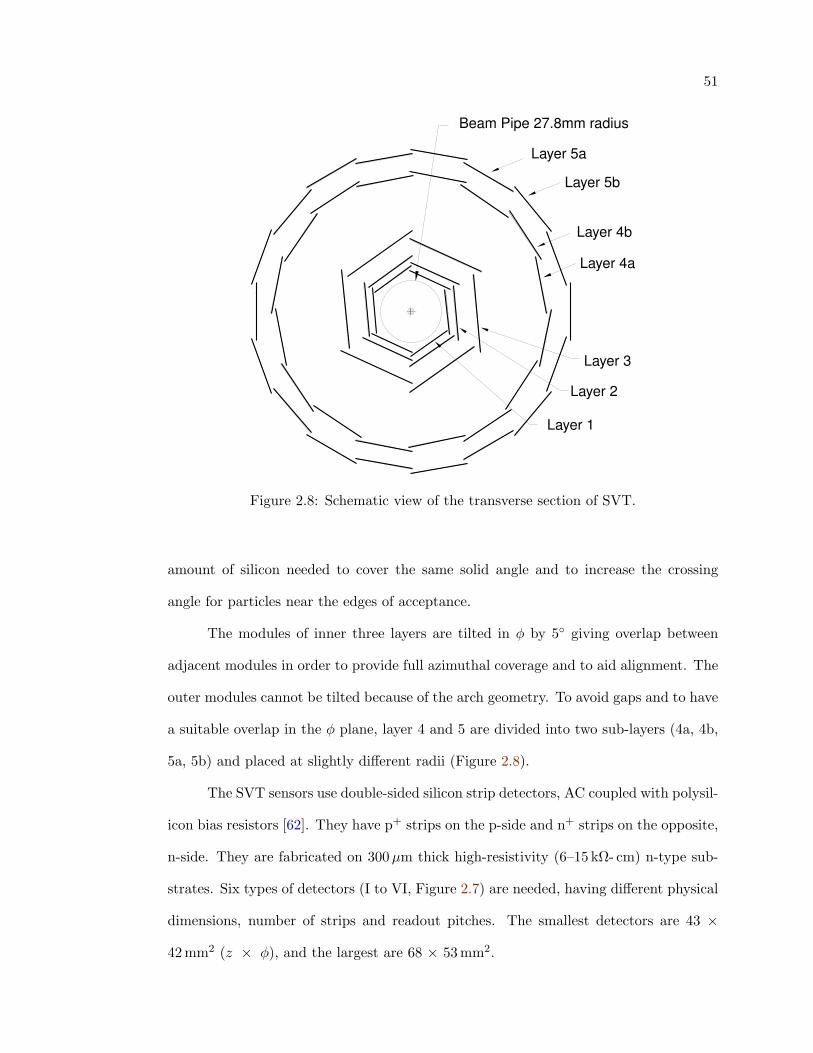
51

Beam Pipe 27.8mm radius

Layer 5a

Layer 5b

Layer 4b

Layer 4a

Layer 3

Layer 2

Layer 1

Figure 2.8: Schematic view of the transverse section of SVT.

amount of silicon needed to cover the same solid angle and to increase the crossing

angle for particles near the edges of acceptance.

The modules of inner three layers are tilted in φ by 5 giving overlap between

adjacent modules in order to provide full azimuthal coverage and to aid alignment. The

outer modules cannot be tilted because of the arch geometry. To avoid gaps and to have

a suitable overlap in the φ plane, layer 4 and 5 are divided into two sub-layers (4a, 4b,

5a, 5b) and placed at slightly different radii (Figure 2.8).

The SVT sensors use double-sided silicon strip detectors, AC coupled with polysil-

icon bias resistors [62]. They have p+ strips on the p-side and n+ strips on the opposite,

n-side. They are fabricated on 300µm thick high-resistivity (6–15 kΩ- cm) n-type sub-

strates. Six types of detectors (I to VI, Figure 2.7) are needed, having different physical

dimensions, number of strips and readout pitches. The smallest detectors are 43 ×

42 mm2 (z × φ), and the largest are 68 × 53 mm2.

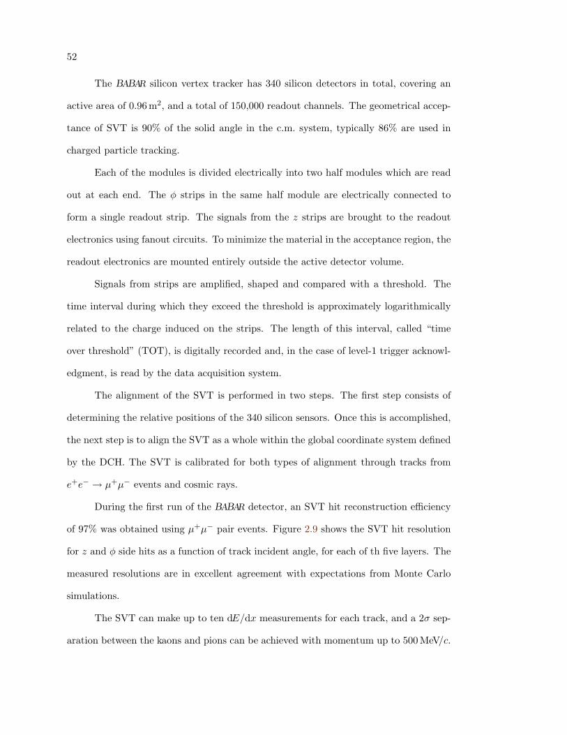
52

The BABAR silicon vertex tracker has 340 silicon detectors in total, covering an

active area of 0.96 m2, and a total of 150,000 readout channels. The geometrical accep-

tance of SVT is 90% of the solid angle in the c.m. system, typically 86% are used in

charged particle tracking.

Each of the modules is divided electrically into two half modules which are read

out at each end. The φ strips in the same half module are electrically connected to

form a single readout strip. The signals from the z strips are brought to the readout

electronics using fanout circuits. To minimize the material in the acceptance region, the

readout electronics are mounted entirely outside the active detector volume.

Signals from strips are amplified, shaped and compared with a threshold. The

time interval during which they exceed the threshold is approximately logarithmically

related to the charge induced on the strips. The length of this interval, called “time

over threshold” (TOT), is digitally recorded and, in the case of level-1 trigger acknowl-

edgment, is read by the data acquisition system.

The alignment of the SVT is performed in two steps. The first step consists of

determining the relative positions of the 340 silicon sensors. Once this is accomplished,

the next step is to align the SVT as a whole within the global coordinate system defined

by the DCH. The SVT is calibrated for both types of alignment through tracks from

e+e− → µ+µ− events and cosmic rays.

During the first run of the BABAR detector, an SVT hit reconstruction efficiency

of 97% was obtained using µ+µ− pair events. Figure 2.9 shows the SVT hit resolution

for z and φ side hits as a function of track incident angle, for each of th five layers. The

measured resolutions are in excellent agreement with expectations from Monte Carlo

simulations.

The SVT can make up to ten dE/dx measurements for each track, and a 2σ sep-

aration between the kaons and pions can be achieved with momentum up to 500MeV/c.

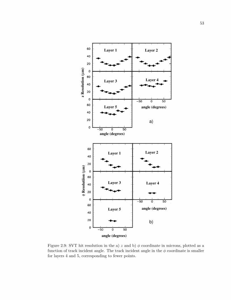
53

angle (degrees)

angle (degrees)

φ R

esol

utiio

n (µ

m)

Layer 1 Layer 2

Layer 3 Layer 4

Layer 5

b)

Layer 1

Layer 3

Layer 5

Layer 2

Layer 4

angle (degrees)

angle (degrees)

z R

esol

utio

n (µ

m)

a)

Figure 2.9: SVT hit resolution in the a) z and b) φ coordinate in microns, plotted as afunction of track incident angle. The track incident angle in the φ coordinate is smallerfor layers 4 and 5, corresponding to fewer points.

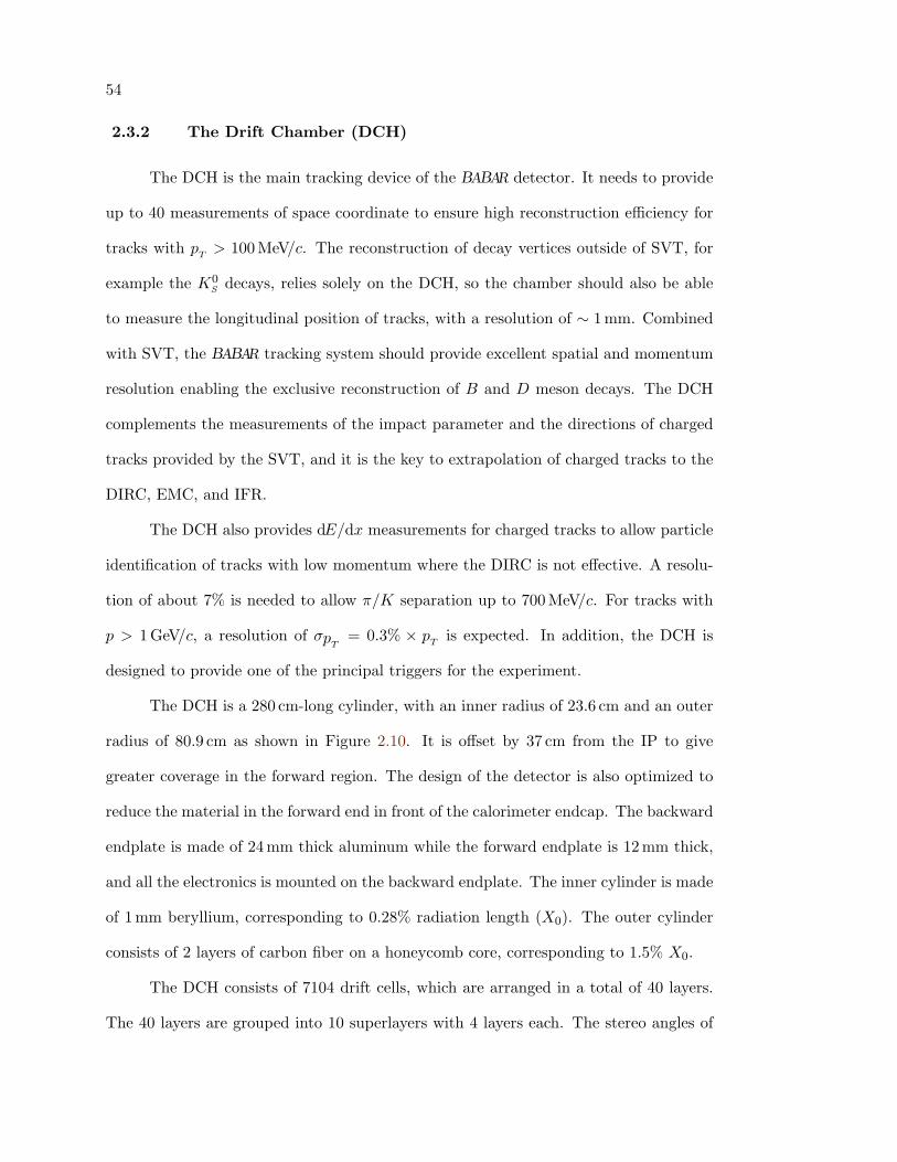
54

2.3.2 The Drift Chamber (DCH)

The DCH is the main tracking device of the BABAR detector. It needs to provide

up to 40 measurements of space coordinate to ensure high reconstruction efficiency for

tracks with pT > 100 MeV/c. The reconstruction of decay vertices outside of SVT, for

example the K0S decays, relies solely on the DCH, so the chamber should also be able

to measure the longitudinal position of tracks, with a resolution of ∼ 1 mm. Combined

with SVT, the BABAR tracking system should provide excellent spatial and momentum

resolution enabling the exclusive reconstruction of B and D meson decays. The DCH

complements the measurements of the impact parameter and the directions of charged

tracks provided by the SVT, and it is the key to extrapolation of charged tracks to the

DIRC, EMC, and IFR.

The DCH also provides dE/dx measurements for charged tracks to allow particle

identification of tracks with low momentum where the DIRC is not effective. A resolu-

tion of about 7% is needed to allow π/K separation up to 700 MeV/c. For tracks with

p > 1 GeV/c, a resolution of σpT= 0.3% × pT is expected. In addition, the DCH is

designed to provide one of the principal triggers for the experiment.

The DCH is a 280 cm-long cylinder, with an inner radius of 23.6 cm and an outer

radius of 80.9 cm as shown in Figure 2.10. It is offset by 37 cm from the IP to give

greater coverage in the forward region. The design of the detector is also optimized to

reduce the material in the forward end in front of the calorimeter endcap. The backward

endplate is made of 24 mm thick aluminum while the forward endplate is 12mm thick,

and all the electronics is mounted on the backward endplate. The inner cylinder is made

of 1mm beryllium, corresponding to 0.28% radiation length (X0). The outer cylinder

consists of 2 layers of carbon fiber on a honeycomb core, corresponding to 1.5% X0.

The DCH consists of 7104 drift cells, which are arranged in a total of 40 layers.

The 40 layers are grouped into 10 superlayers with 4 layers each. The stereo angles of

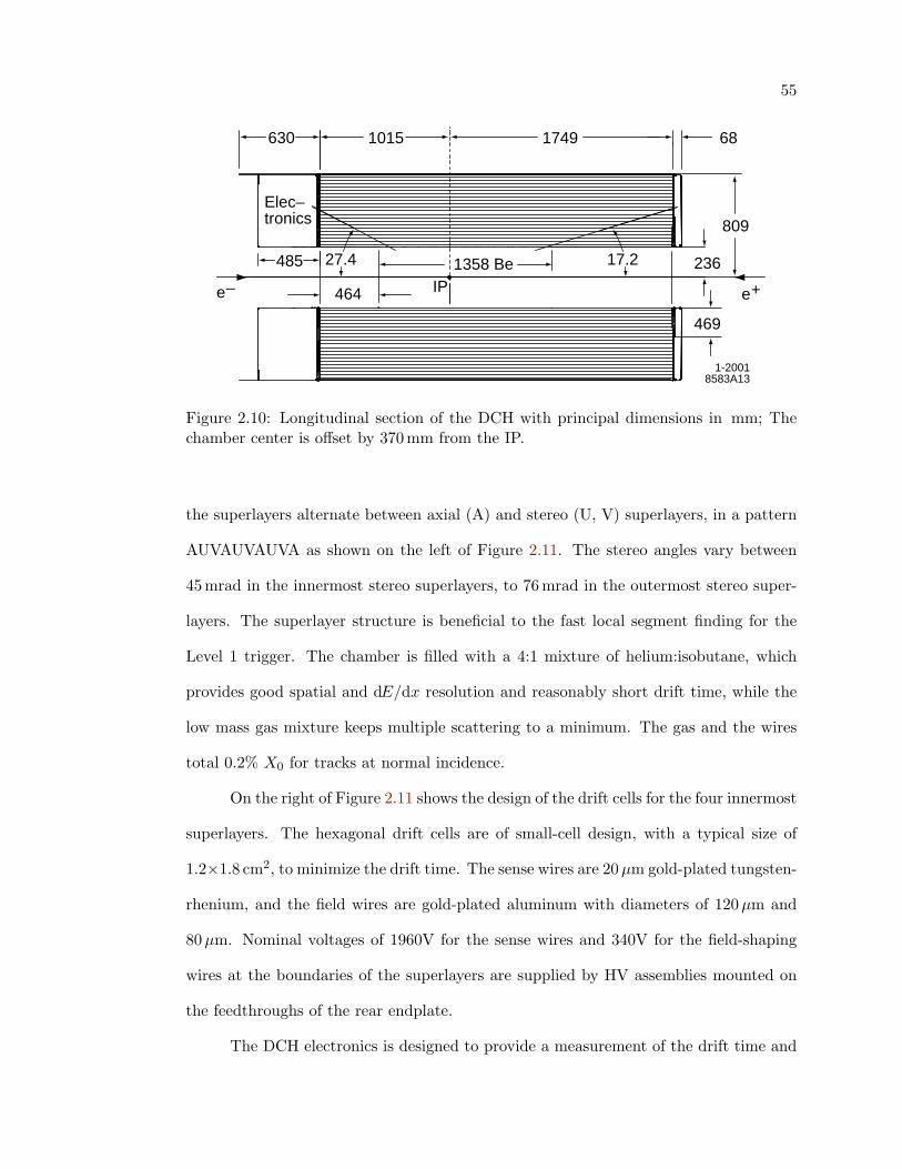
55

IP236

469

1015

1358 Be

1749

809

485

630 68

27.4

464

Elec–tronics

17.2

e– e+

1-20018583A13

Figure 2.10: Longitudinal section of the DCH with principal dimensions in mm; Thechamber center is offset by 370mm from the IP.

the superlayers alternate between axial (A) and stereo (U, V) superlayers, in a pattern

AUVAUVAUVA as shown on the left of Figure 2.11. The stereo angles vary between

45 mrad in the innermost stereo superlayers, to 76 mrad in the outermost stereo super-

layers. The superlayer structure is beneficial to the fast local segment finding for the

Level 1 trigger. The chamber is filled with a 4:1 mixture of helium:isobutane, which

provides good spatial and dE/dx resolution and reasonably short drift time, while the

low mass gas mixture keeps multiple scattering to a minimum. The gas and the wires

total 0.2% X0 for tracks at normal incidence.

On the right of Figure 2.11 shows the design of the drift cells for the four innermost

superlayers. The hexagonal drift cells are of small-cell design, with a typical size of

1.2×1.8 cm2, to minimize the drift time. The sense wires are 20µm gold-plated tungsten-

rhenium, and the field wires are gold-plated aluminum with diameters of 120µm and

80µm. Nominal voltages of 1960V for the sense wires and 340V for the field-shaping

wires at the boundaries of the superlayers are supplied by HV assemblies mounted on

the feedthroughs of the rear endplate.

The DCH electronics is designed to provide a measurement of the drift time and

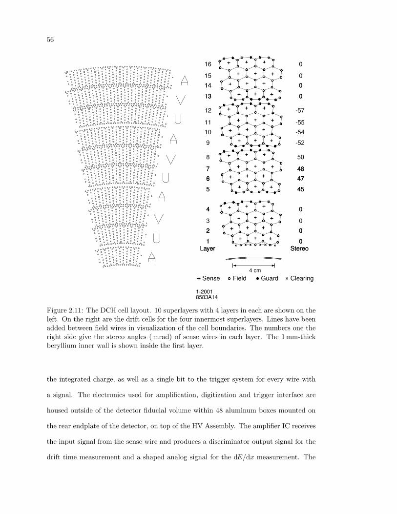
56

0Stereo

1 Layer

0Stereo

1 Layer

0 2 0 2 0 2

0 3

0 4 0 4

45 5 45 5

47 6 47 6 47 6

48 7 48 7

50 8

-52 9

-5410

-5511

-5712

013 013

014 014

015

016

4 cmSense Field Guard Clearing

1-2001 8583A14

Figure 2.11: The DCH cell layout. 10 superlayers with 4 layers in each are shown on theleft. On the right are the drift cells for the four innermost superlayers. Lines have beenadded between field wires in visualization of the cell boundaries. The numbers one theright side give the stereo angles ( mrad) of sense wires in each layer. The 1 mm-thickberyllium inner wall is shown inside the first layer.

the integrated charge, as well as a single bit to the trigger system for every wire with

a signal. The electronics used for amplification, digitization and trigger interface are

housed outside of the detector fiducial volume within 48 aluminum boxes mounted on

the rear endplate of the detector, on top of the HV Assembly. The amplifier IC receives

the input signal from the sense wire and produces a discriminator output signal for the

drift time measurement and a shaped analog signal for the dE/dx measurement. The

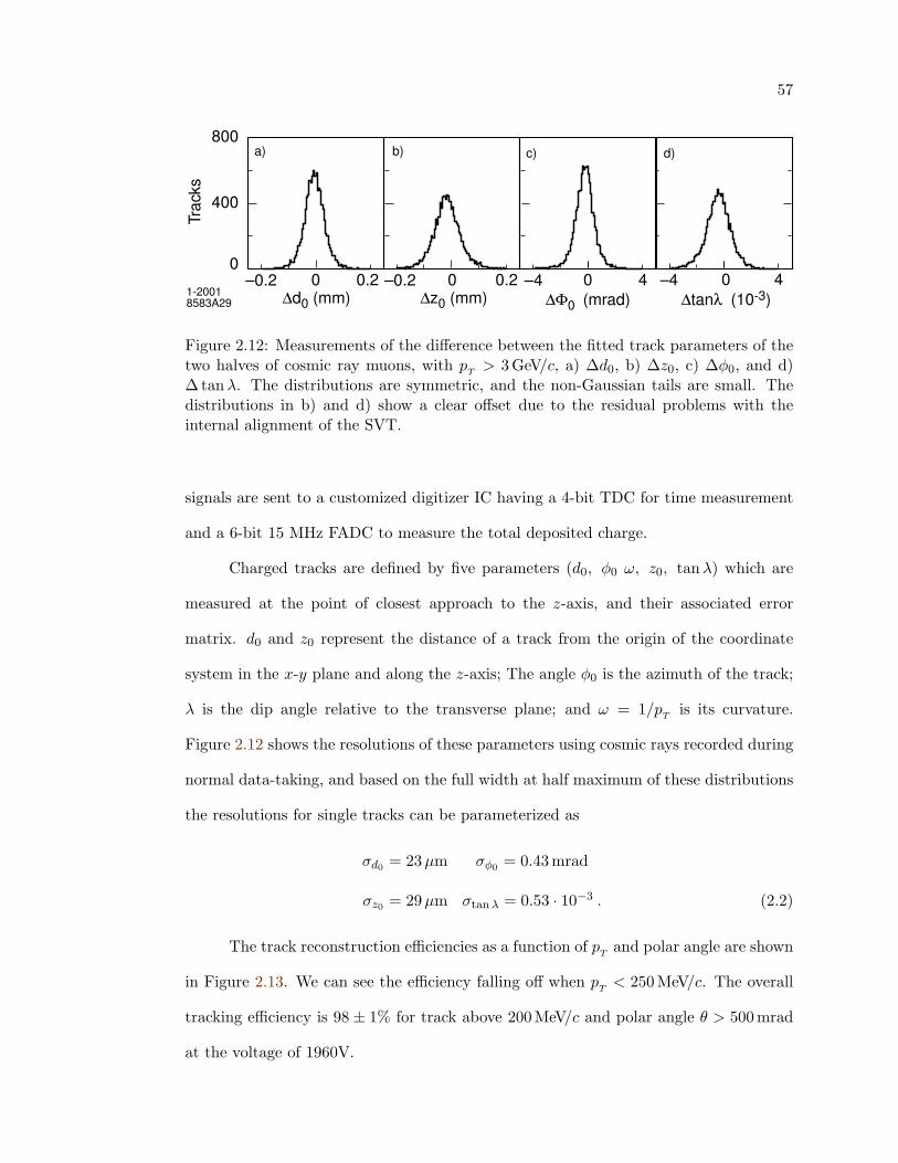
57

0

400

800

Trac

ks

–0.2 0 0.2 –0.2 0.20 ∆z0 (mm)

–4 40∆tanλ (10-3)

∆d0 (mm) ∆Φ0 (mrad)1-2001 8583A29

a) b)

–4 0 4

c) d)

Figure 2.12: Measurements of the difference between the fitted track parameters of thetwo halves of cosmic ray muons, with pT > 3 GeV/c, a) ∆d0, b) ∆z0, c) ∆φ0, and d)∆ tanλ. The distributions are symmetric, and the non-Gaussian tails are small. Thedistributions in b) and d) show a clear offset due to the residual problems with theinternal alignment of the SVT.

signals are sent to a customized digitizer IC having a 4-bit TDC for time measurement

and a 6-bit 15 MHz FADC to measure the total deposited charge.

Charged tracks are defined by five parameters (d0, φ0 ω, z0, tanλ) which are

measured at the point of closest approach to the z-axis, and their associated error

matrix. d0 and z0 represent the distance of a track from the origin of the coordinate

system in the x-y plane and along the z-axis; The angle φ0 is the azimuth of the track;

λ is the dip angle relative to the transverse plane; and ω = 1/pT is its curvature.

Figure 2.12 shows the resolutions of these parameters using cosmic rays recorded during

normal data-taking, and based on the full width at half maximum of these distributions

the resolutions for single tracks can be parameterized as

σd0 = 23µm σφ0 = 0.43 mrad

σz0 = 29µm σtan λ = 0.53 · 10−3 . (2.2)

The track reconstruction efficiencies as a function of pT and polar angle are shown

in Figure 2.13. We can see the efficiency falling off when pT < 250 MeV/c. The overall

tracking efficiency is 98± 1% for track above 200MeV/c and polar angle θ > 500 mrad

at the voltage of 1960V.

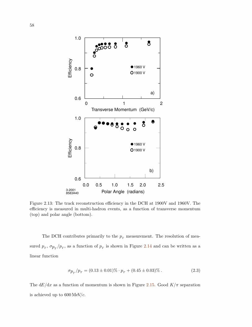
58

Polar Angle (radians)

Transverse Momentum (GeV/c)

Effi

cien

cy

0.6

0.8

1.0

0.6

0.8

1.0

Effi

cien

cy

0 1 2

3-2001 8583A40

1960 V

1900 V

a)

1960 V

1900 V

b)

0.0 0.5 1.51.0 2.0 2.5

Figure 2.13: The track reconstruction efficiency in the DCH at 1900V and 1960V. Theefficiency is measured in multi-hadron events, as a function of transverse momentum(top) and polar angle (bottom).

The DCH contributes primarily to the pT measurement. The resolution of mea-

sured pT , σpT/pT , as a function of pT is shown in Figure 2.14 and can be written as a

linear function

σpT/pT = (0.13± 0.01)% · pT + (0.45± 0.03)% . (2.3)

The dE/dx as a function of momentum is shown in Figure 2.15. Good K/π separation

is achieved up to 600 MeV/c.

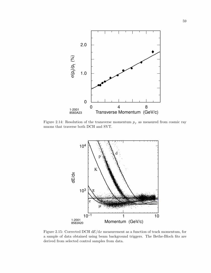
59

0

1.0

2.0

0 4 8Transverse Momentum (GeV/c)

σ(p t

)/pt

(%)

1-2001 8583A23

Figure 2.14: Resolution of the transverse momentum pT as measured from cosmic raymuons that traverse both DCH and SVT.

104

103

10–1 101

eµ

π

K

pd

dE/d

x

Momentum (GeV/c)1-2001 8583A20

Figure 2.15: Corrected DCH dE/dx measurement as a function of track momentum, fora sample of data obtained using beam background triggers. The Bethe-Bloch fits arederived from selected control samples from data.

60

2.3.3 DIRC

One important key to the study of CP violation is the ability to tag the flavor of

one of the B meson via the cascade decay b → c → s by identifying the final product

kaons, which have a momentum up to about 2 GeV/c, with most of them below 1 GeV/c.

In addition, pions and kaons from rare B decays, which are the subject of this work,

must be well separated. The momenta of those tracks are between 1.7 and 4.2 GeV/c

with a strong momentum-polar angle correlation because of the c.m. system boost.

The particle identification (PID) system of the BABAR detector is a new kind of

ring-imaging Cerenkov detector, Detector of Internally Reflected Cerenkov light (the

DIRC), which relies on the detection of Cerenkov photons trapped in the radiator due

to total internal reflection [63]. It is expected to provide better than 4σ π/K separation

for all tracks from B meson decays in the momentum range 0.7∼4.2GeV/c.

The DIRC is based on the principle that the angles of light are maintained upon

reflection from a flat surface. The overall design is shown in Figure 2.16, which illustrates

the principles of light production, transport, and imaging. The DIRC radiator consists

of 144 long, straight bars of fused synthetic silica (mean index of refraction n = 1.473)

with rectangular section, arranged in a 12-sided polygonal barrel with each bar box

containing 12 bars (see Figure 2.17). The bars are 1.7 cm thick, 3.5 cm wide and 4.9m

long. Each bar is assembled from four 1.225 m pieces that are glued end-to-end.

For particles with β ≈ 1, some photons will always lie within the total internal

reflection limit, and will be transported to either one or both ends of the bar. A mirror

is placed at the forward end to reflect the photons towards the backward readout end.

Each bar has a fused silica wedge glued to it at the readout end to reflect photons at

large angles relative to the bar axis so as to reduce the size of the required detection

surface and recover those photons that would otherwise be lost due to internal reflection

at the fused silica/water interface. The twelve wedges in a bar box are glued to a

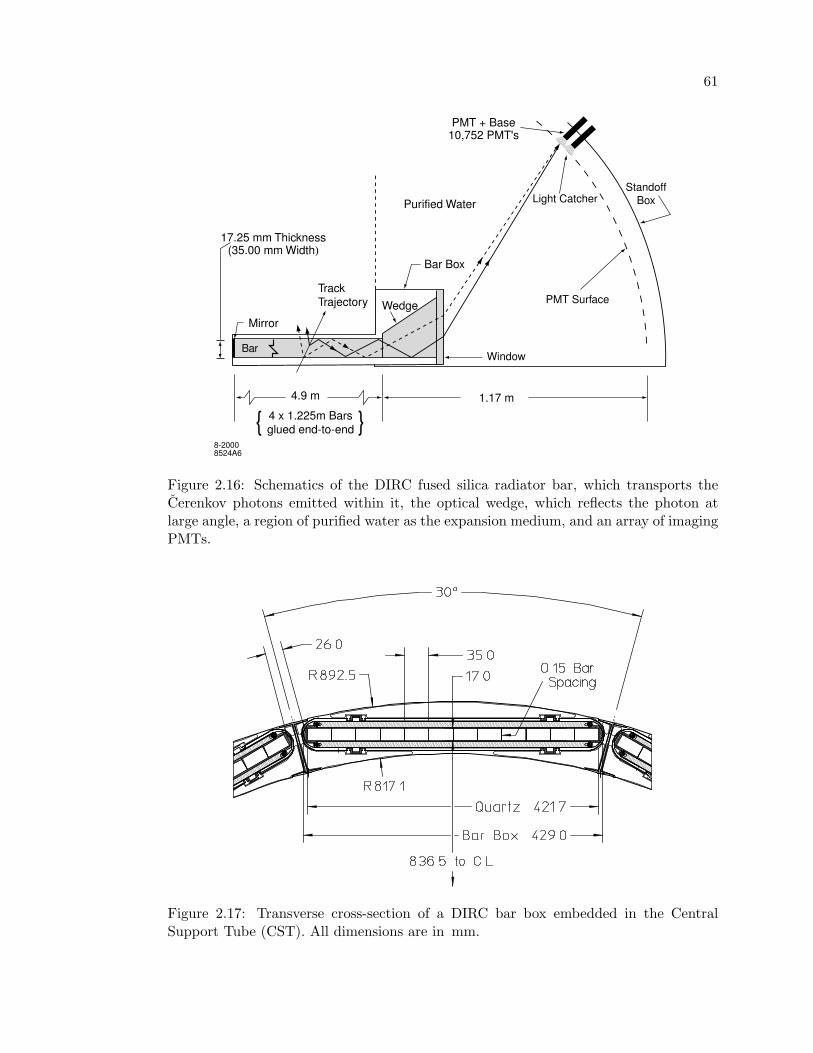
61

Mirror

4.9 m

4 x 1.225m Bars glued end-to-end

Purified Water

WedgeTrack Trajectory

17.25 mm Thickness (35.00 mm Width)

Bar Box

PMT + Base 10,752 PMT's

Light Catcher

PMT Surface

Window

Standoff Box

Bar

1.17 m

8-2000 8524A6

Figure 2.16: Schematics of the DIRC fused silica radiator bar, which transports theCerenkov photons emitted within it, the optical wedge, which reflects the photon atlarge angle, a region of purified water as the expansion medium, and an array of imagingPMTs.

Figure 2.17: Transverse cross-section of a DIRC bar box embedded in the CentralSupport Tube (CST). All dimensions are in mm.

62

common 10 mm-thick fused silica window, which provides the interface and seal to the

purified water in the expansion region, called the standoff box. Water is chosen as

the expansion medium because it is inexpensive and has an average index of refraction

(n≈1.346) reasonably close to that of fused silica. The standoff box is made of stainless

steel, consisting of a cone, cylinder, and 12 sectors of PMTs, and it contains about 6,000

liters of purified water.

The photons are detected by an array of densely packed photo-multiplier tubes

(PMTs), each surrounded by reflecting light catcher cones to capture light. The PMTs

are placed at a distance of about 1.2 m from the bar end on the 12 PMT sectors at

the rear of the standoff box. Each of the 12 PMT sectors contains 896 PMTs with

29 mm-diameter.

The DIRC occupies 80mm of radial space and a total of about 17% radiation

length. The radiator bars cover a solid angle corresponding to about 94% of the azimuth

and 83% of the c.m. polar angle cosine.

The DIRC front-end electronics (FEE) is designed to measure the arrival time

of each Cerenkov photon detected by the PMT array to an accuracy of 1.5 ns limited

by the intrinsic transit time spread of the PMTs. The DIRC FEE is mounted on the

outside of the standoff box. Each of the 168 Front-end Boards (DFBs) processes 64

PMT inputs and contain 8 custom analogue chips, 4 TDCs and one 8-bit FADC.

The Cerenkov angle information is reconstructed from the position and arrival

time of the PMT signals. The timing measurements are used to suppress background

hits and to separate photons from different tracks. Figure 2.18 shows the pattern of

Cerenkov photon before and after the timing cut.

The emission angle and arrival time of the Cerenkov photons are transformed

into the Cerenkov coordinate system, θc, the Cerenkov angle, φc, the azimuthal angle

of a Cerenkov photon around the track direction, and δt, the difference between the

measured and expected photon arrival time. An unbinned maximum likelihood method

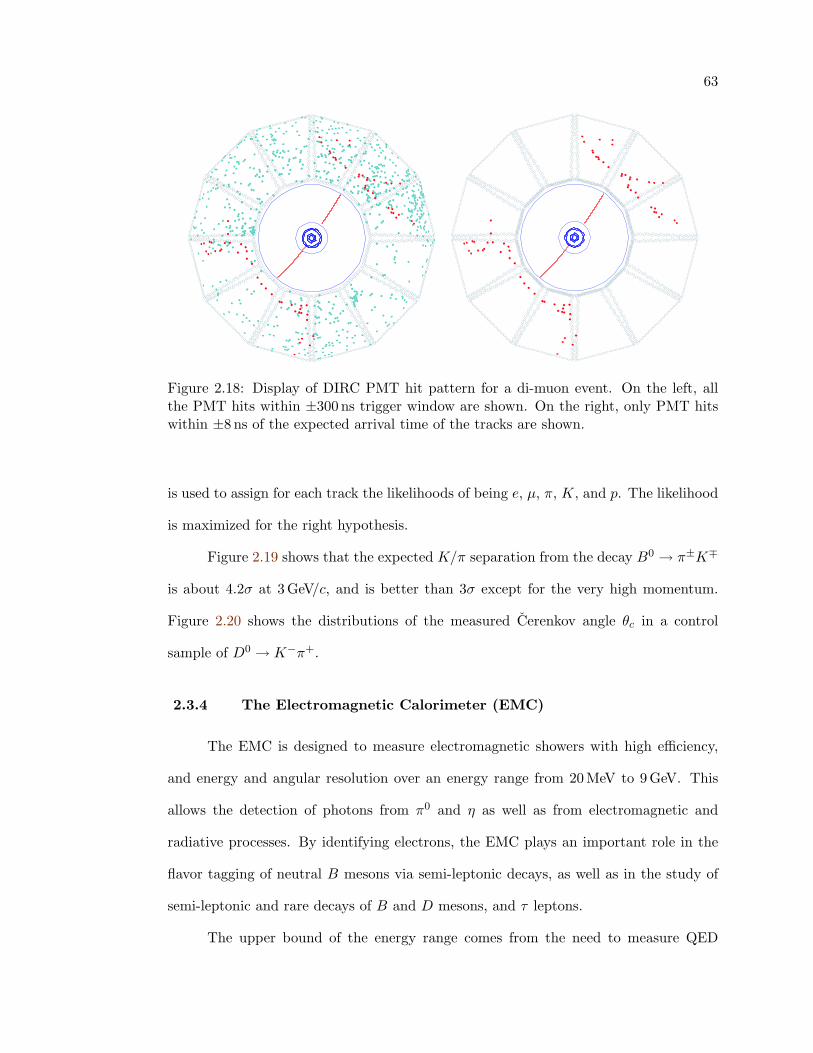
63

Figure 2.18: Display of DIRC PMT hit pattern for a di-muon event. On the left, allthe PMT hits within ±300 ns trigger window are shown. On the right, only PMT hitswithin ±8 ns of the expected arrival time of the tracks are shown.

is used to assign for each track the likelihoods of being e, µ, π, K, and p. The likelihood

is maximized for the right hypothesis.

Figure 2.19 shows that the expected K/π separation from the decay B0 → π±K∓

is about 4.2σ at 3 GeV/c, and is better than 3σ except for the very high momentum.

Figure 2.20 shows the distributions of the measured Cerenkov angle θc in a control

sample of D0 → K−π+.

2.3.4 The Electromagnetic Calorimeter (EMC)

The EMC is designed to measure electromagnetic showers with high efficiency,

and energy and angular resolution over an energy range from 20MeV to 9 GeV. This

allows the detection of photons from π0 and η as well as from electromagnetic and

radiative processes. By identifying electrons, the EMC plays an important role in the

flavor tagging of neutral B mesons via semi-leptonic decays, as well as in the study of

semi-leptonic and rare decays of B and D mesons, and τ leptons.

The upper bound of the energy range comes from the need to measure QED

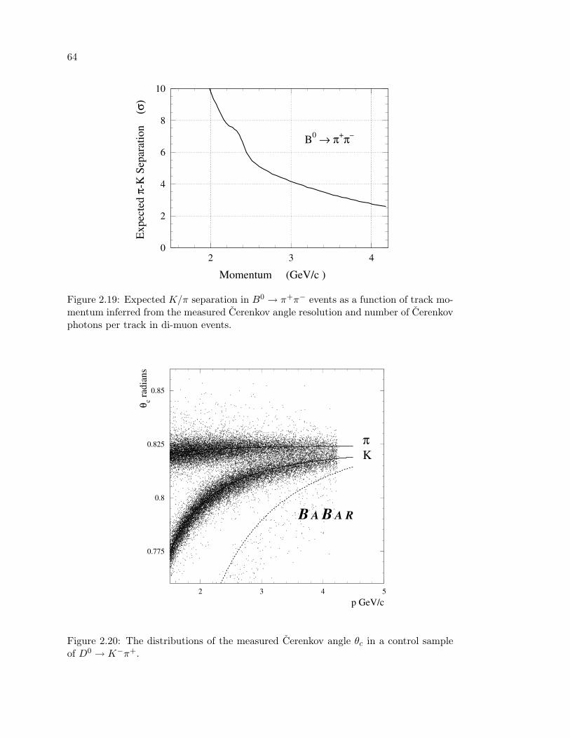
64

B0 → π+π–

Momentum (GeV/c )

Exp

ecte

d π-

K S

epar

atio

n

(σ)

0

2

4

6

8

10

2 3 4

Figure 2.19: Expected K/π separation in B0 → π+π− events as a function of track mo-mentum inferred from the measured Cerenkov angle resolution and number of Cerenkovphotons per track in di-muon events.

p GeV/c

θ c rad

ians

B A B A R

πK

0.775

0.8

0.825

0.85

2 3 4 5

Figure 2.20: The distributions of the measured Cerenkov angle θc in a control sampleof D0 → K−π+.

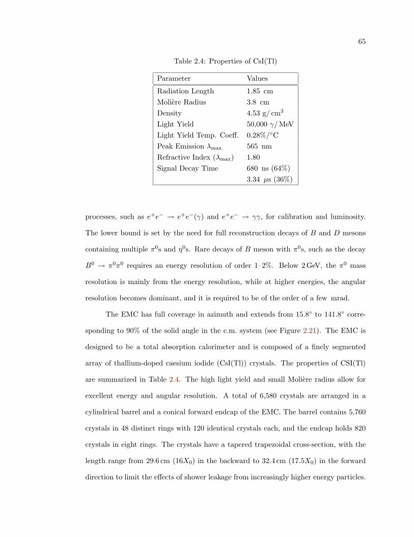
65

Table 2.4: Properties of CsI(Tl)

Parameter Values

Radiation Length 1.85 cmMoliere Radius 3.8 cmDensity 4.53 g/ cm3

Light Yield 50,000 γ/ MeVLight Yield Temp. Coeff. 0.28%/CPeak Emission λmax 565 nmRefractive Index (λmax) 1.80Signal Decay Time 680 ns (64%)

3.34 µs (36%)

processes, such as e+e− → e+e−(γ) and e+e− → γγ, for calibration and luminosity.

The lower bound is set by the need for full reconstruction decays of B and D mesons

containing multiple π0s and η0s. Rare decays of B meson with π0s, such as the decay

B0 → π0π0 requires an energy resolution of order 1–2%. Below 2GeV, the π0 mass

resolution is mainly from the energy resolution, while at higher energies, the angular

resolution becomes dominant, and it is required to be of the order of a few mrad.

The EMC has full coverage in azimuth and extends from 15.8 to 141.8 corre-

sponding to 90% of the solid angle in the c.m. system (see Figure 2.21). The EMC is

designed to be a total absorption calorimeter and is composed of a finely segmented

array of thallium-doped caesium iodide (CsI(Tl)) crystals. The properties of CSI(Tl)

are summarized in Table 2.4. The high light yield and small Moliere radius allow for

excellent energy and angular resolution. A total of 6,580 crystals are arranged in a

cylindrical barrel and a conical forward endcap of the EMC. The barrel contains 5,760

crystals in 48 distinct rings with 120 identical crystals each, and the endcap holds 820

crystals in eight rings. The crystals have a tapered trapezoidal cross-section, with the

length range from 29.6 cm (16X0) in the backward to 32.4 cm (17.5X0) in the forward

direction to limit the effects of shower leakage from increasingly higher energy particles.

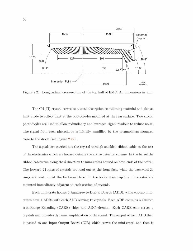
66

11271375920

1555 2295

2359

1801

558

1979

22.7˚

26.8˚

15.8˚

Interaction Point 1-2001 8572A03

38.2˚

External Support

Figure 2.21: Longitudinal cross-section of the top half of EMC. All dimensions in mm.

The CsI(Tl) crystal serves as a total absorption scintillating material and also as

light guide to collect light at the photodiodes mounted at the rear surface. Two silicon

photodiodes are used to allow redundancy and averaged signal readout to reduce noise.

The signal from each photodiode is initially amplified by the preamplifiers mounted

close to the diode (see Figure 2.22).

The signals are carried out the crystal through shielded ribbon cable to the rest

of the electronics which are housed outside the active detector volume. In the barrel the

ribbon cables run along the θ direction to mini-crates housed on both ends of the barrel.

The forward 24 rings of crystals are read out at the front face, while the backward 24

rings are read out at the backward face. In the forward endcap the mini-crates are

mounted immediately adjacent to each section of crystals.

Each mini-crate houses 6 Analogue-to-Digital Boards (ADB), while endcap mini-

crates have 4 ADBs with each ADB serving 12 crystals. Each ADB contains 3 Custom

AutoRange Encoding (CARE) chips and ADC circuits. Each CARE chip serves 4

crystals and provides dynamic amplification of the signal. The output of each ADB then

is passed to one Input-Output-Board (IOB) which serves the mini-crate, and then is

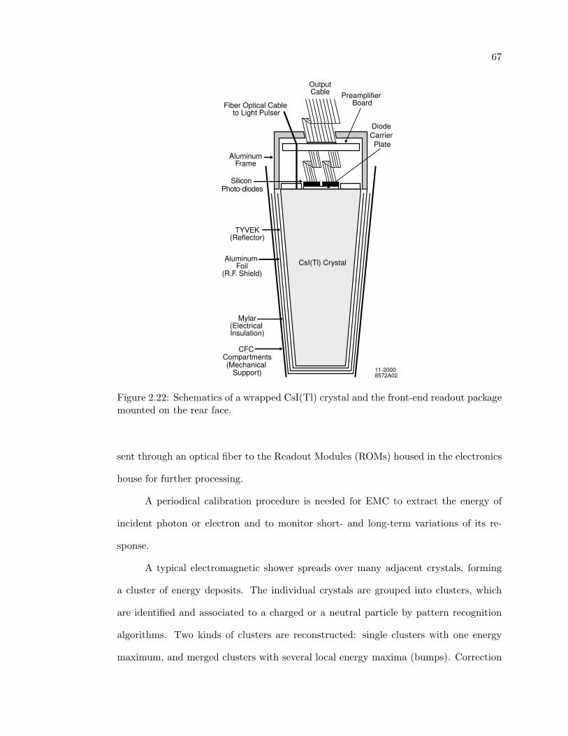
67

CsI(Tl) Crystal

Diode Carrier Plate

Silicon Photo-diodes

Preamplifier BoardFiber Optical Cable

to Light Pulser

Aluminum Frame

TYVEK (Reflector)

Mylar (Electrical Insulation)

Aluminum Foil

(R.F. Shield)

CFC Compartments (Mechanical

Support)

Output Cable

11-2000 8572A02

Figure 2.22: Schematics of a wrapped CsI(Tl) crystal and the front-end readout packagemounted on the rear face.

sent through an optical fiber to the Readout Modules (ROMs) housed in the electronics

house for further processing.

A periodical calibration procedure is needed for EMC to extract the energy of

incident photon or electron and to monitor short- and long-term variations of its re-

sponse.

A typical electromagnetic shower spreads over many adjacent crystals, forming

a cluster of energy deposits. The individual crystals are grouped into clusters, which

are identified and associated to a charged or a neutral particle by pattern recognition

algorithms. Two kinds of clusters are reconstructed: single clusters with one energy

maximum, and merged clusters with several local energy maxima (bumps). Correction

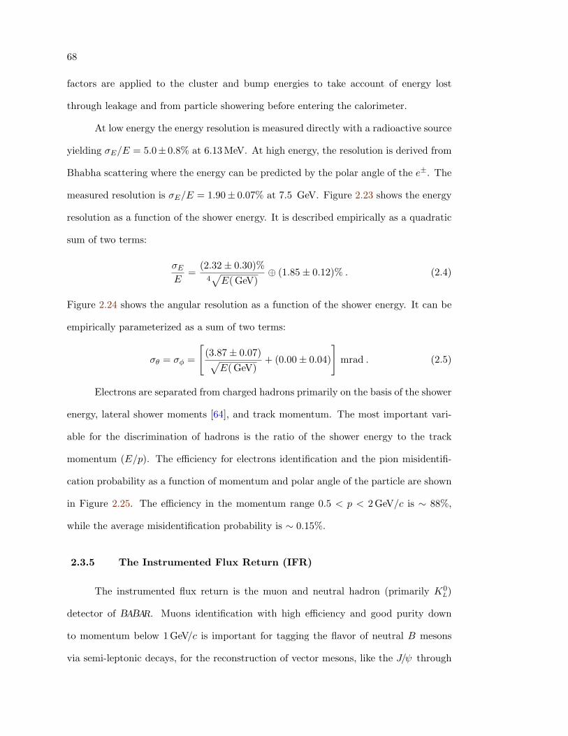
68

factors are applied to the cluster and bump energies to take account of energy lost

through leakage and from particle showering before entering the calorimeter.

At low energy the energy resolution is measured directly with a radioactive source

yielding σE/E = 5.0± 0.8% at 6.13MeV. At high energy, the resolution is derived from

Bhabha scattering where the energy can be predicted by the polar angle of the e±. The

measured resolution is σE/E = 1.90± 0.07% at 7.5 GeV. Figure 2.23 shows the energy

resolution as a function of the shower energy. It is described empirically as a quadratic

sum of two terms:

σE

E=

(2.32± 0.30)%4√E( GeV)

⊕ (1.85± 0.12)% . (2.4)

Figure 2.24 shows the angular resolution as a function of the shower energy. It can be

empirically parameterized as a sum of two terms:

σθ = σφ =

[(3.87± 0.07)√

E( GeV)+ (0.00± 0.04)

]mrad . (2.5)

Electrons are separated from charged hadrons primarily on the basis of the shower

energy, lateral shower moments [64], and track momentum. The most important vari-

able for the discrimination of hadrons is the ratio of the shower energy to the track

momentum (E/p). The efficiency for electrons identification and the pion misidentifi-

cation probability as a function of momentum and polar angle of the particle are shown

in Figure 2.25. The efficiency in the momentum range 0.5 < p < 2 GeV/c is ∼ 88%,

while the average misidentification probability is ∼ 0.15%.

2.3.5 The Instrumented Flux Return (IFR)

The instrumented flux return is the muon and neutral hadron (primarily K0L)

detector of BABAR. Muons identification with high efficiency and good purity down

to momentum below 1 GeV/c is important for tagging the flavor of neutral B mesons

via semi-leptonic decays, for the reconstruction of vector mesons, like the J/ψ through

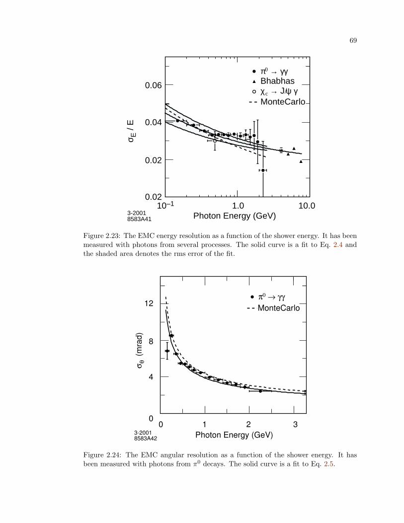
69

γγ→0πBhabhas

c

MonteCarloγψ J/→χ

3-20018583A41 Photon Energy (GeV)

10–1 1.0 10.0

σE /

E

0.02

0.02

0.04

0.06

Figure 2.23: The EMC energy resolution as a function of the shower energy. It has beenmeasured with photons from several processes. The solid curve is a fit to Eq. 2.4 andthe shaded area denotes the rms error of the fit.

3-2001 8583A42 Photon Energy (GeV)

0 1 2 3

σ θ (

mra

d)

0

4

8

12γγ → 0π

MonteCarlo

Figure 2.24: The EMC angular resolution as a function of the shower energy. It hasbeen measured with photons from π0 decays. The solid curve is a fit to Eq. 2.5.

70

40 80 120

± e

± π

0.00.000

0.002

0.004

0.006

0.008

0.010

0.000

0.002

0.004

0.006

0.008

0.010

Effi

cien

cy

0.0

0.2

0.4

0.6

0.8

1.0

Effi

cien

cy

0.0

0.2

0.4

0.6

0.8

1.0

± e

± π

0 1 2Momentum (GeV/c)

Polar Angle (degrees)3-2001 8583A43

a)

b)

Figure 2.25: EMC electron efficiency and pion misidentification probability as a functiona) the particle momentum and b) the polar angle, measured in the laboratory system.The electron efficiency is measured using radiative Bhabhas and e+e− → e+e−e+e−

events. The pion misidentification probability is measured for selected charged pionsfrom K0

S decays and three-prong τ decays.

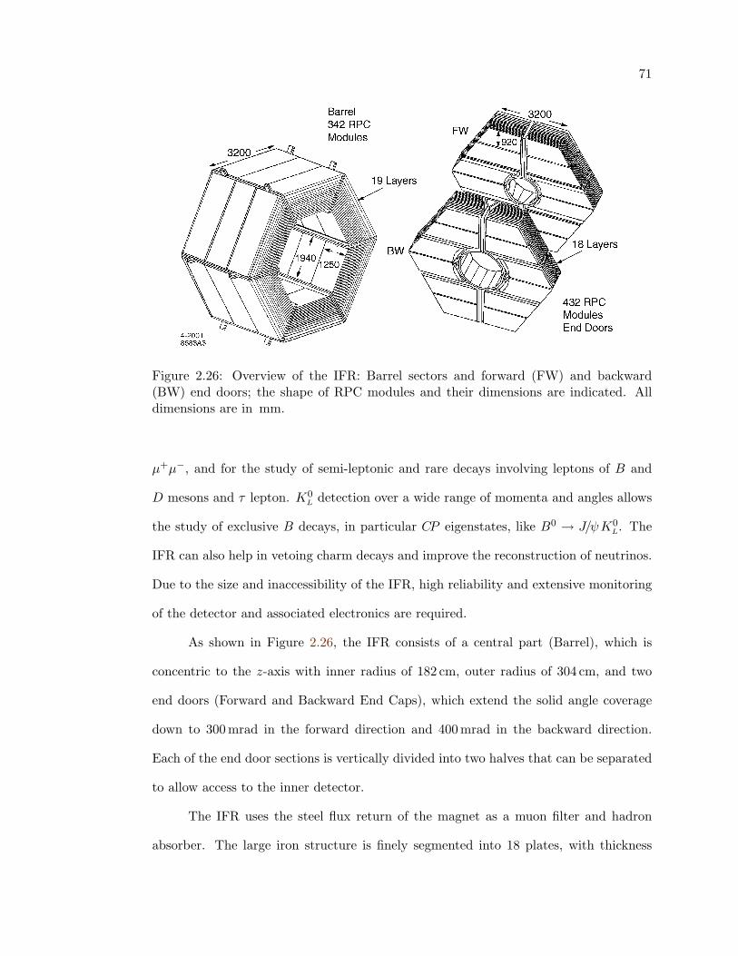
71

Figure 2.26: Overview of the IFR: Barrel sectors and forward (FW) and backward(BW) end doors; the shape of RPC modules and their dimensions are indicated. Alldimensions are in mm.

µ+µ−, and for the study of semi-leptonic and rare decays involving leptons of B and

D mesons and τ lepton. K0L detection over a wide range of momenta and angles allows

the study of exclusive B decays, in particular CP eigenstates, like B0 → J/ψK0L. The

IFR can also help in vetoing charm decays and improve the reconstruction of neutrinos.

Due to the size and inaccessibility of the IFR, high reliability and extensive monitoring

of the detector and associated electronics are required.

As shown in Figure 2.26, the IFR consists of a central part (Barrel), which is

concentric to the z-axis with inner radius of 182 cm, outer radius of 304 cm, and two

end doors (Forward and Backward End Caps), which extend the solid angle coverage

down to 300 mrad in the forward direction and 400 mrad in the backward direction.

Each of the end door sections is vertically divided into two halves that can be separated

to allow access to the inner detector.

The IFR uses the steel flux return of the magnet as a muon filter and hadron

absorber. The large iron structure is finely segmented into 18 plates, with thickness

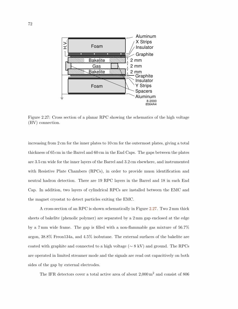
72

AluminumX StripsInsulator

2 mm

GraphiteInsulator

SpacersY Strips

Aluminum

H.V

.

Foam

Bakelite

BakeliteGas

Foam

Graphite

2 mm2 mm

8-2000 8564A4

Figure 2.27: Cross section of a planar RPC showing the schematics of the high voltage(HV) connection.

increasing from 2 cm for the inner plates to 10 cm for the outermost plates, giving a total

thickness of 65 cm in the Barrel and 60 cm in the End Caps. The gaps between the plates

are 3.5 cm wide for the inner layers of the Barrel and 3.2 cm elsewhere, and instrumented

with Resistive Plate Chambers (RPCs), in order to provide muon identification and

neutral hadron detection. There are 19 RPC layers in the Barrel and 18 in each End

Cap. In addition, two layers of cylindrical RPCs are installed between the EMC and

the magnet cryostat to detect particles exiting the EMC.

A cross-section of an RPC is shown schematically in Figure 2.27. Two 2 mm thick

sheets of bakelite (phenolic polymer) are separated by a 2 mm gap enclosed at the edge

by a 7 mm wide frame. The gap is filled with a non-flammable gas mixture of 56.7%

argon, 38.8% Freon134a, and 4.5% isobutane. The external surfaces of the bakelite are

coated with graphite and connected to a high voltage (∼ 8 kV) and ground. The RPCs

are operated in limited streamer mode and the signals are read out capacitively on both

sides of the gap by external electrodes.

The IFR detectors cover a total active area of about 2,000m2 and consist of 806

73

RPC modules, 57 in each of the six barrel sectors, 108 in each of the four half end

doors, and 32 in the two cylindrical layers. More than 25 different shapes and sizes of

the RPCs are needed. In the barrel sectors, the gaps between the steels plates extend

375 cm in the z direction and vary in width from 180 cm to 320 cm. Three modules are

needed to cover the whole area as shown in Figure 2.26.

Each barrel module has 32 strips perpendicular to the beam axis to measure the

z coordinate and 96 strips in the orthogonal direction extending over three modules to

measure φ. Each of the four half end doors is divided into three sections. Each of these

section is covered by two RPC modules that are joined to form a larger chamber with

horizontal and vertical readout strips.

RPCs detect streamers from ionizing particles via capacitive readout strips. Data

from strips are sent to Front End Card (FEC). Each FEC serves 16 input strips. Signals

from the 3,300 FECs are transmitted to eight custom front end crates, from where the

data are buffered and sent through an optical fiber to the DAQ system upon receiving

a signal from the trigger system.

One-dimensional IFR clusters are formed as a group of adjacent hits in one of the

two readout coordinates. The cluster position is defined as the centroid of the strips in

the cluster. Two-dimensional clusters are formed by joining one-dimensional clusters (of

the same readout coordinate) in different layers. In each sector, two-dimensional clusters

in different coordinates are combined into three-dimensional clusters provided there are

fewer than three layers missing in one of the two coordinates. The clusters are matched

to tracks reconstructed in the DCH, and a number of variables are defined for each IFR

cluster associated with a charged track to discriminate muons from charged hadrons.

Those variables include nλ, the total number of interaction lengths traversed from the

IP to the last RPC layer with an associated cluster, ∆nλ, the difference between nλ and

the predicted penetration depth for a muon of the same momentum and angle, etc [65].

K0L’s and other neutral hadrons are identified as clusters that are not associated with a

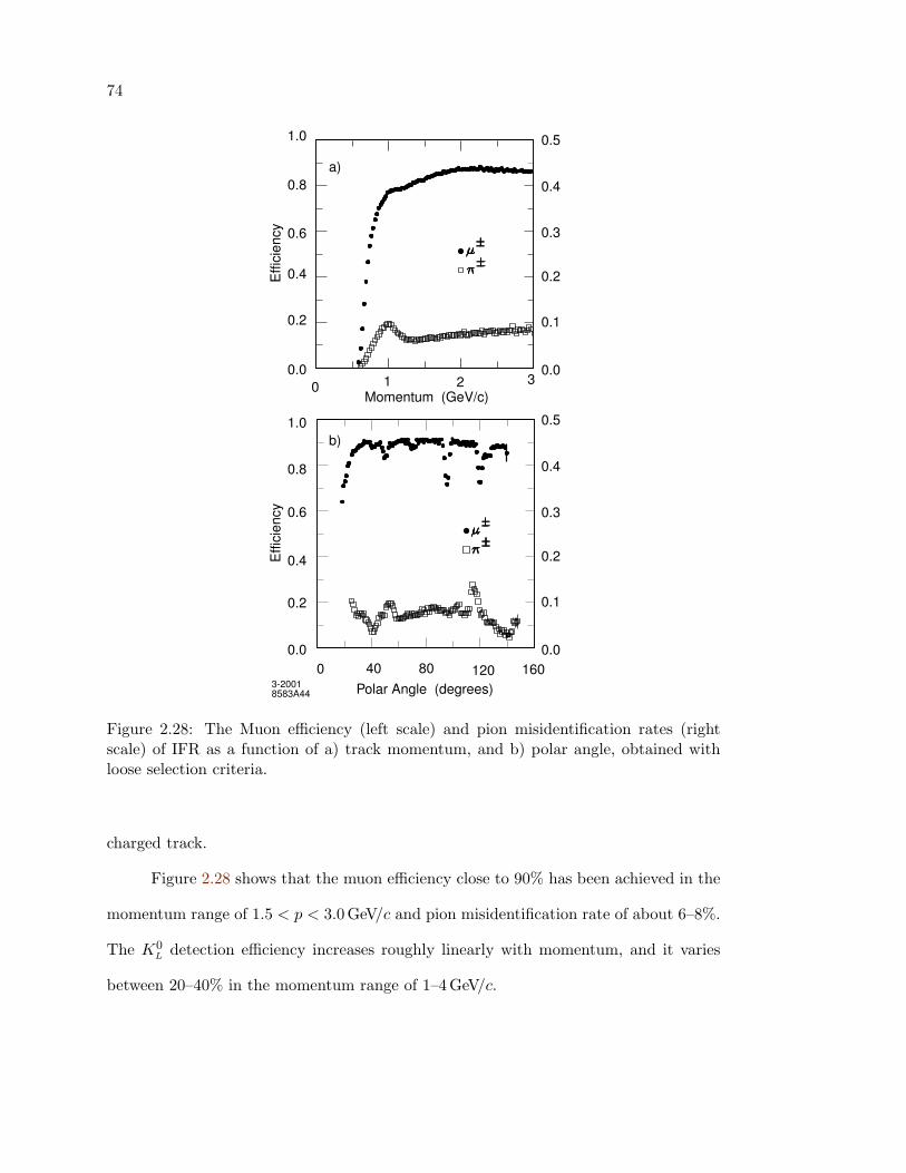
74

Momentum (GeV/c)

Effi

cien

cyE

ffici

ency

0.0

0.2

0.4

0.6

0.8

1.0

0 1 2 30.0

0.1

0.2

0.3

0.4

0.5

0.0

0.1

0.2

0.3

0.4

0.5

3-2001 8583A44

a)

b)

Polar Angle (degrees)

0.0

0.2

0.4

0.6

0.8

1.0

0 40 80 120 160

Figure 2.28: The Muon efficiency (left scale) and pion misidentification rates (rightscale) of IFR as a function of a) track momentum, and b) polar angle, obtained withloose selection criteria.

charged track.

Figure 2.28 shows that the muon efficiency close to 90% has been achieved in the

momentum range of 1.5 < p < 3.0 GeV/c and pion misidentification rate of about 6–8%.

The K0L detection efficiency increases roughly linearly with momentum, and it varies

between 20–40% in the momentum range of 1–4GeV/c.

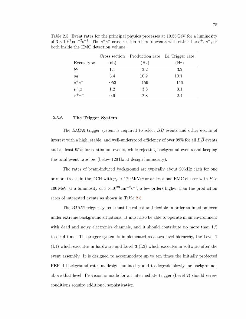
75

Table 2.5: Event rates for the principal physics processes at 10.58 GeV for a luminosityof 3× 1033 cm−2s−1. The e+e− cross-section refers to events with either the e+, e−, orboth inside the EMC detection volume.

Cross section Production rate L1 Trigger rateEvent type (nb) (Hz) (Hz)

bb 1.1 3.2 3.2qq 3.4 10.2 10.1e+e− ∼53 159 156µ+µ− 1.2 3.5 3.1τ+τ− 0.9 2.8 2.4

2.3.6 The Trigger System

The BABAR trigger system is required to select BB events and other events of

interest with a high, stable, and well-understood efficiency of over 99% for all BB events

and at least 95% for continuum events, while rejecting background events and keeping

the total event rate low (below 120 Hz at design luminosity).

The rates of beam-induced background are typically about 20 kHz each for one

or more tracks in the DCH with pT > 129 MeV/c or at least one EMC cluster with E >

100 MeV at a luminosity of 3 × 1033 cm−2s−1, a few orders higher than the production

rates of interested events as shown in Table 2.5.

The BABAR trigger system must be robust and flexible in order to function even

under extreme background situations. It must also be able to operate in an environment

with dead and noisy electronics channels, and it should contribute no more than 1%

to dead time. The trigger system is implemented as a two-level hierarchy, the Level 1

(L1) which executes in hardware and Level 3 (L3) which executes in software after the

event assembly. It is designed to accommodate up to ten times the initially projected

PEP-II background rates at design luminosity and to degrade slowly for backgrounds

above that level. Provision is made for an intermediate trigger (Level 2) should severe

conditions require additional sophistication.

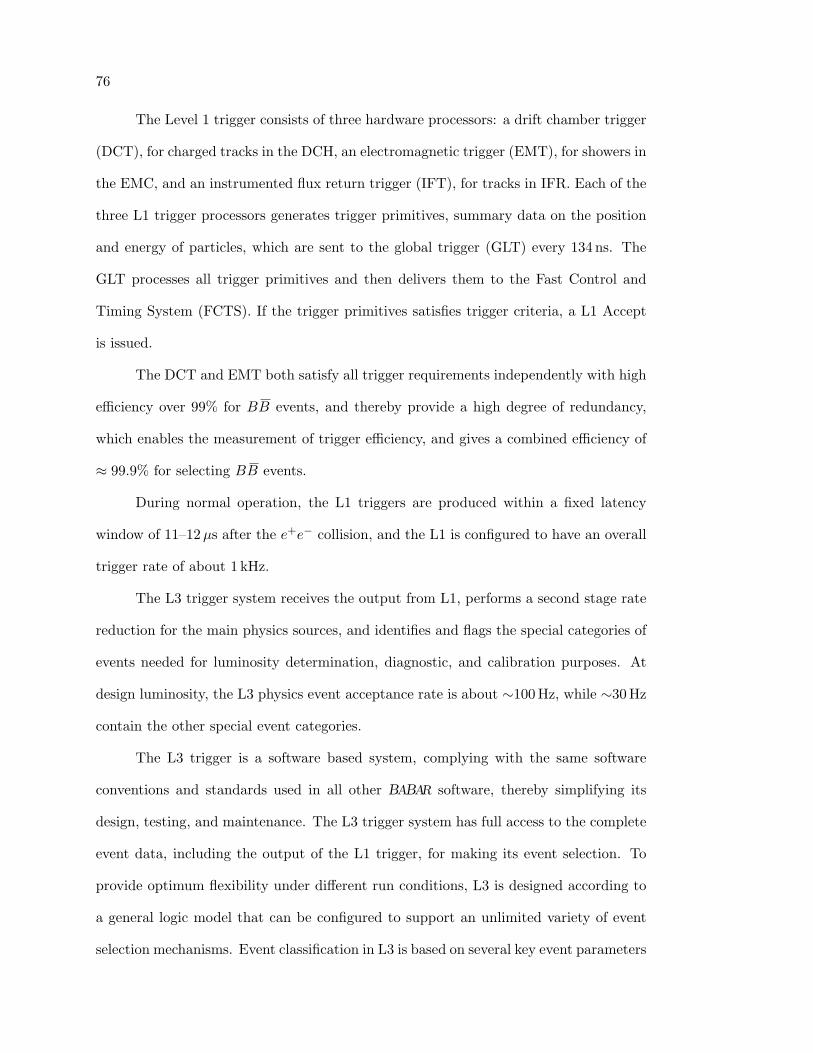
76

The Level 1 trigger consists of three hardware processors: a drift chamber trigger

(DCT), for charged tracks in the DCH, an electromagnetic trigger (EMT), for showers in

the EMC, and an instrumented flux return trigger (IFT), for tracks in IFR. Each of the

three L1 trigger processors generates trigger primitives, summary data on the position

and energy of particles, which are sent to the global trigger (GLT) every 134 ns. The

GLT processes all trigger primitives and then delivers them to the Fast Control and

Timing System (FCTS). If the trigger primitives satisfies trigger criteria, a L1 Accept

is issued.

The DCT and EMT both satisfy all trigger requirements independently with high

efficiency over 99% for BB events, and thereby provide a high degree of redundancy,

which enables the measurement of trigger efficiency, and gives a combined efficiency of

≈ 99.9% for selecting BB events.

During normal operation, the L1 triggers are produced within a fixed latency

window of 11–12µs after the e+e− collision, and the L1 is configured to have an overall

trigger rate of about 1 kHz.

The L3 trigger system receives the output from L1, performs a second stage rate

reduction for the main physics sources, and identifies and flags the special categories of

events needed for luminosity determination, diagnostic, and calibration purposes. At

design luminosity, the L3 physics event acceptance rate is about ∼100 Hz, while ∼30 Hz

contain the other special event categories.

The L3 trigger is a software based system, complying with the same software

conventions and standards used in all other BABAR software, thereby simplifying its

design, testing, and maintenance. The L3 trigger system has full access to the complete

event data, including the output of the L1 trigger, for making its event selection. To

provide optimum flexibility under different run conditions, L3 is designed according to

a general logic model that can be configured to support an unlimited variety of event

selection mechanisms. Event classification in L3 is based on several key event parameters

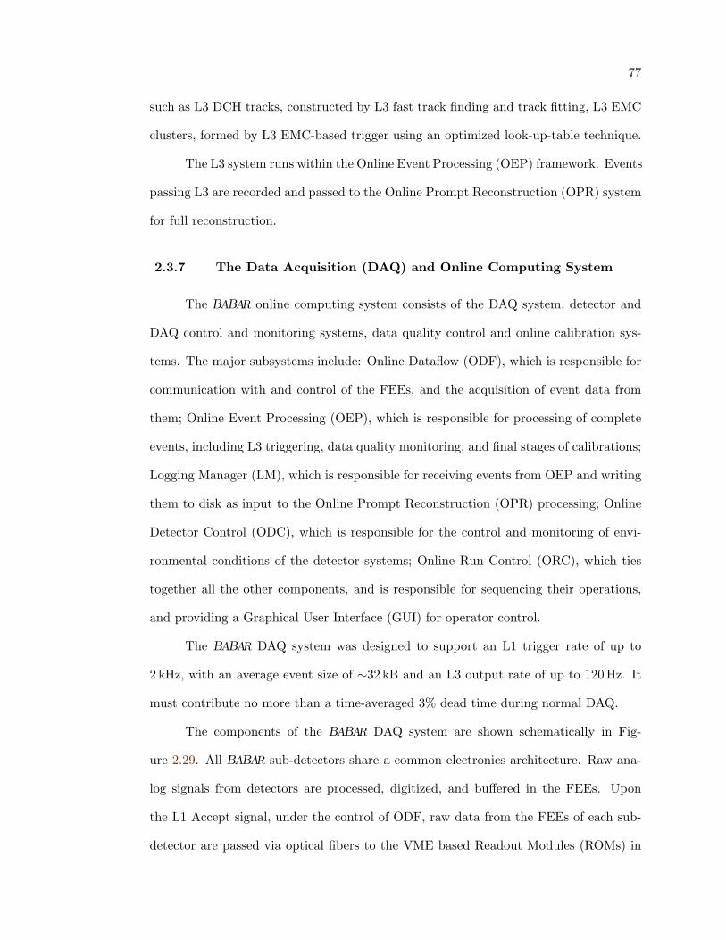
77

such as L3 DCH tracks, constructed by L3 fast track finding and track fitting, L3 EMC

clusters, formed by L3 EMC-based trigger using an optimized look-up-table technique.

The L3 system runs within the Online Event Processing (OEP) framework. Events

passing L3 are recorded and passed to the Online Prompt Reconstruction (OPR) system

for full reconstruction.

2.3.7 The Data Acquisition (DAQ) and Online Computing System

The BABAR online computing system consists of the DAQ system, detector and

DAQ control and monitoring systems, data quality control and online calibration sys-

tems. The major subsystems include: Online Dataflow (ODF), which is responsible for

communication with and control of the FEEs, and the acquisition of event data from

them; Online Event Processing (OEP), which is responsible for processing of complete

events, including L3 triggering, data quality monitoring, and final stages of calibrations;

Logging Manager (LM), which is responsible for receiving events from OEP and writing

them to disk as input to the Online Prompt Reconstruction (OPR) processing; Online

Detector Control (ODC), which is responsible for the control and monitoring of envi-

ronmental conditions of the detector systems; Online Run Control (ORC), which ties

together all the other components, and is responsible for sequencing their operations,

and providing a Graphical User Interface (GUI) for operator control.

The BABAR DAQ system was designed to support an L1 trigger rate of up to

2 kHz, with an average event size of ∼32 kB and an L3 output rate of up to 120 Hz. It

must contribute no more than a time-averaged 3% dead time during normal DAQ.

The components of the BABAR DAQ system are shown schematically in Fig-

ure 2.29. All BABAR sub-detectors share a common electronics architecture. Raw ana-

log signals from detectors are processed, digitized, and buffered in the FEEs. Upon

the L1 Accept signal, under the control of ODF, raw data from the FEEs of each sub-

detector are passed via optical fibers to the VME based Readout Modules (ROMs) in

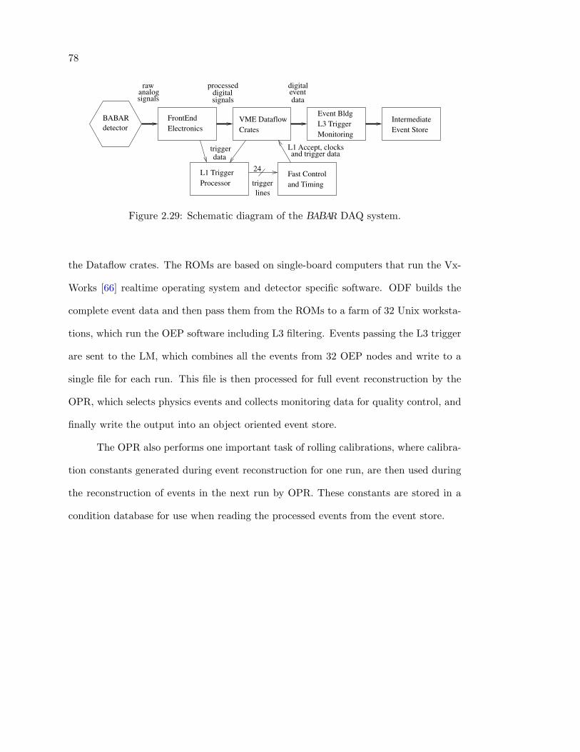
78

FrontEndElectronics

VME DataflowCrates

L1 TriggerProcessor

Fast Controland Timing

Event BldgL3 TriggerMonitoring

IntermediateEvent Store

dataeventdigitalraw

signalsanalog

signals

processeddigital

data

BABARdetector

trigger

24

L1 Accept, clocksand trigger data

linestrigger

Figure 2.29: Schematic diagram of the BABAR DAQ system.

the Dataflow crates. The ROMs are based on single-board computers that run the Vx-

Works [66] realtime operating system and detector specific software. ODF builds the

complete event data and then pass them from the ROMs to a farm of 32 Unix worksta-

tions, which run the OEP software including L3 filtering. Events passing the L3 trigger

are sent to the LM, which combines all the events from 32 OEP nodes and write to a

single file for each run. This file is then processed for full event reconstruction by the

OPR, which selects physics events and collects monitoring data for quality control, and

finally write the output into an object oriented event store.

The OPR also performs one important task of rolling calibrations, where calibra-

tion constants generated during event reconstruction for one run, are then used during

the reconstruction of events in the next run by OPR. These constants are stored in a

condition database for use when reading the processed events from the event store.

Chapter 3

Analysis Techniques

In this chapter, we will discuss major analysis techniques used for this work.

First we have an overview of the BABAR software and analysis framework in Sec. 3.1.

Sec. 3.2 lists the data samples used for this work, and then we will go through the

criteria for particle reconstruction and identification, reconstruction of B daughters,

and B candidate selection, in Sec. 3.3, 3.4, and 3.5, respectively. We summarize our

main analysis method to extract final results, the Maximum Likelihood (ML) fit, and

relevant topics in Sec. 3.6, and finally we will discuss systematic uncertainties of our

analyses in Sec. 3.7.

A blind analysis technique [67] is used for all the modes studied in this work.

This means we conceal the signal region of the data sample until the analysis has been

optimized for best signal-to-background ratio, and all the problems have been fixed. A

false signal could be enhanced if the selection criteria are made to do so intentionally.

By not looking at the signal region, this blind procedure reduces the risk of any such bias

introduced while tuning the analysis parameters. When the analysis has been finalized,

we are ready for unblinding to get analysis results from the full data sample.

3.1 The BABAR Software and Analysis Tools

The BABAR software environment includes online and offline systems. The online

system is responsible for real-time control of the detector, monitoring, calibration, and

80

data acquisition as summarized in Sec. 2.3.7 on page 77.

The offline system consists of tools for simulation, reconstruction, data quality

control, physics analysis, etc. Both online and offline systems are based on Object-

Oriented (OO) design and use C++ [68] as their primary programming language. Codes

are divided into modules, each of which performs a particular task, such that they can

be reused for many purposes and across the two systems.

The offline tools share the same OO architecture in the BABAR Application Frame-

work [69], which is a flexible, general purpose structure to enforce certain well designed

standards of code behavior, using the Tool Command Language, TCL [70], as the user

interface. The Framework is implemented as a class library, which defines the form of

all user classes and the interactions between these classes.

The building blocks in the BABAR Framework are objects called modules. All the

module classes inherit from the class AppModule so they share the same interface and

can interact to each other in a coherent way. Four types of module are defined: input

modules and output modules to control the input and output of data, filter modules to

terminate or redirect subsequent data processing, and processing modules to take data

from an event, run specific algorithms, and finally put the resulting data back to the

event for later use.

Several related modules form a Framework sequence to be executed in an ordered

manner to provide a defined service to the Framework, such as the reconstruction of a

sub-detector. A path is formed by sequences and individual modules to control the flow

of execution in the Framework. The actual BABAR offline job is done with an execution

path, which starts from an active input module, ends at an active output module, and

consists of one or more paths. Each module, sequence, or path, can be enabled (default)

or disabled. Only those enabled can be seen by the Framework and executed.

81

Monte Carlo Simulation

The BABAR Monte Carlo (MC) Simulation produces simulated data for the signal

and background studies in the blind analysis stage, and for cross check after unblinding.

Several stages are required to produce these simulated data:

(1) Generation of the physics event.

Several event generators are used in the MC simulation for different purposes.

They are interfaced to the BABAR Framework through GenFwkInt (Generators-

Framework Interface) package [71]. The most commonly used generators are

EvtGen [72] for simulating exclusive physics processes in decays of B mesons,

and Jetset [73] for other inclusive B decays, and generic continuum events.

(2) Particle transport and calculation of energy deposits in the detector.

The propagation of the generated particles through the BABAR detector is sim-

ulated by BOGUS, the BABAR Object-oriented Unified Simulation program [74],

which is implemented via GEANT4 [75], a toolkit for the simulation of the passage

of particles through matter.

The first two stages are done in one executable called BgsApp. The program

produces an output file in a data structure called GHits, which contains the

(idealized) energy deposited by the particles passing through the detector, and

the locations of the deposit.

(3) Overlaying of backgrounds and digitization of the energy deposits.

The idealized GHits data is then processed by a package called SimApp. This

program overlays backgrounds with the GHits and produces signals which look

as exactly as possible as the real data collected by the detector electronics.

The backgrounds overlaid are not simulated. They are actual detector event

samples recorded with a random trigger.

82

(4) Reconstruction.

The raw data from simulation is reconstructed with a package called Bear, in the

same way as the real data is reconstructed in OPR by a package called Elf. The

Bear application (BearApp) runs the full reconstruction chain, invoking the re-

construction modules within the SVT, DCH, DIRC, EMC and IFR sub-systems.

Each reconstruction module uses pattern recognition, fitting algorithms, etc. to

produce a set of objects representing the reconstructed information, such as can-

didates of cluster, track, etc. The output is various candidate lists of clusters,

tracks, which can be used in physics analyses.

MC data for this work are produced in this BgsApp-SimApp-Bear three-step pro-

cedure. A new scheme, called MOOSE (Monolithic Object-Oriented Simulation Exe-

cutable) [76], which finishes all the stages in one step, is now available for Simulation

Production (SP).

Beta Toolkit

Beta [77] is a toolkit for use with BABAR data to do physics analysis. It consists

of multiple packages, including:

• Beta, basic package of the base classes, etc.

• BetaTools and BetaCoreTools, analysis level tools.

• BetaUser, sample package which can be used to build user-level analysis tools.

and many more.

In this level, there is usually no need to access raw data, rather, Beta provides

lists of candidate, which is the Beta representation of particle that may have existed

in the event in question. For example, charged tracks can be candidate pions, and

neutral clusters can be candidate photons. The output of vertexing two candidates

is a composite candidate for a particle which decays into those two candidates. The

83

vertexing is one of the operators Beta provides to combine one or more candidates to

form new ones. Other operators include four-vector addition, geometric or kinematic

fitting, etc.

Beta also defines higher level classes for physics analysis. Candidates can be fil-

tered by selectors which apply some “cuts” to select appropriate hypotheses. Selectors

include many different types from general PID selectors based on various algorithms, to

composite selectors which build, for example, D and B mesons, and to specific selectors

tailored for individual analyses. Associators can be used to link daughter and mother

particles in decay trees, and to associate charged track candidates with neutral cluster

candidates, etc., or to associate reconstructed candidates with their appropriate MC

truth candidates for MC data.

Based on Beta, the BetaTools and BetaCoreTools packages [78] provide a diverse

set of tools essential to many physics analyses. The BetaCoreTools package contains

classes that calculate event shape variables (those associated with an event, or part of

an event), utility functions for tasks like boosting a candidate and all its decay products,

and simple vertexing (adding 4 momenta). The BetaTools package contains classes that

provide MC truth association with reconstructed candidates, micro smearing/killing

classes for efficiency corrections of MC data, and various candidate selectors and other

useful tools not in the core package.

Users can build their own analysis tools on top of Beta, making use of the existing

physics analysis tools, to add new features specific to their own needs. BetaUser package

is provided as a template for such purpose. Analyses in this work are done on the Beta

level using a package called Q2BUser [79], which provides a generic framework for the

study of charmless-2-body decays. The event reconstruction, selection, and output has

been standardized for all the decays of this type, and tcl configuration files specific to

individual decay modes are used to control the package to use appropriate data, perform

corresponding analysis, and produce desirable output for each of them.

84

CompositionTools

As mentioned before, Beta provides a whole collection of operators and selectors

to reconstruct composite particles from existing candidates. CompositionTools [80],

which consists of many such tools, is the package used to produce lists of composite

candidates describing a given decay reaction.

The reconstruction of composite candidates in this package is performed in two

separated and independent steps:

• Combinatorics.

Possible combinations of candidates are determined according to the decay tree

based on the charge and type of input candidates. A generic combinatoric

engine is implemented.

• Selection.

Several selection criteria are applied to those combinations, and those passing

the selections are output into the final list of composite candidates corresponding

to the decay tree. Several generic vertexing/kinematic fitters and vertexers have

been implemented.

All the classes of CompositionTools inherit from CompositeSelector, which can

take up to 5 lists of daughters, their mass hypotheses, and a set of selection criteria, re-

construct decay trees in the two steps with generic implementations, and finally store the

composite candidates into an output list for later use. Based on CompositeSelector,

other base composite candidate selector classes include: CompTwoBodySelector, a base

class for selectors of particles decaying to two body, CompV0Selector, a base class for

selectors of long-lived particles (K0s, Λ, etc.), CompB0Selector/CompBSelector, base

classes for selection of neutral and charged Bs.

It is beneficial to have the two-step design of reconstruction and the hierarchy

of selectors. A new selector just needs to have the decay tree specified if other imple-

85

mentations of the selector are quite standard and, if more specific criteria are required,

only those selection functions need to be overridden. It is convenient for selectors to

have several levels of selection criteria for different purposes, and because of the archi-

tecture of the package, it is very easy to implement several similar selectors. Four levels

of criteria are usually defined for selectors: VeryLoose, Loose, Tight, and VeryTight

selectors.

In addition to the selector implementation standards and many base classes, the

CompositionTools package provides a factory of numerous specific selectors already

implemented and validated for many physics analyses.

The Q2BUser package makes use of the base selectors and selectors in the factory

of CompositionTools to reconstruct full B decay trees for charmless (quasi-)two-body

rare B decays with minimal efforts in the actual coding of the selectors and most of the

control and configurations can be done in individual tcl files.

ROOT and RooFit

Higher level data analysis than Beta deals with physics variables which can be

decoupled from the BABAR environments. Common platforms for this final stage of the

whole analysis cycle are PAW, Physics Analysis Workstation [81], and ROOT [82]. PAW,

written in Fortran, was a popular interactive analysis tool in the experimental particle

physics community before ROOT was introduced in 1995.

ROOT is an object-oriented data analysis system written by the creators of PAW.

The ROOT system provides a set of OO frameworks with all the functionality needed

to handle and analyze large amounts of data in a very efficient way. Its programming

language is C++, which is also the command language, and the scripting, or macro,

language of the system because it has a builtin CINT [83] C++ interpreter which can run

C++ codes interpretively. Its class library can be grouped into several categories: base

classes, container classes, histogram classes, tree and ntuple classes, graphics classes,

86

etc., which provides a powerful set of tools capable to do sophisticated experimental

particle physics analysis and beyond.

Analysis packages can also be built upon ROOT infrastructure. One widely used

package in BABAR analysis is RooFit [84], a toolkit for data modeling based on ROOT.

It provides a powerful extension to ROOT for data modeling, fitting, plotting, and data

generating for various studies, which satisfies the needs of BABAR physics analysis. Users

can build their own analysis package based on RooFit and ROOT.

Final analyses for this work are done with Q2BFit [85,86], a fitting package based

on RooFit and ROOT, and working with Q2BUser, for the purpose of charmless rare B

decay analysis. The Q2BFit package provides a general fitting environment for this type

of analysis. In this package, the coding is minimal and the fitter is controlled through

plain ASCII configuration files, which are understandable to the program through the

RooFit interface. Several types of fitting procedures are defined to fulfill different stages

of the final analysis, including distribution shape modeling, plotting, fitting validation,

final branching fraction fitting, time-dependent fitting, etc. Q2BFit, together with other

small scripts and programs, is the main tool to extract our final results.

The BABAR software packages have been developed and improved constantly.

The Software Release Tools (SRT), based on Concurrent Version System (CVS) [87],

are used to manage the release control. Stable versions of packages are given logical

tags. A BABAR software release contains a consistent set of packages, one tagged version

for each of them, together with the libraries and binaries created for various machine

architectures. Users usually create their own working release by checking out a light-

weighted collection of packages of particular releases and then tailor those packages for

their analyses.

In addition to the software and tools mentioned above, BABAR also makes use of

many other available software systems. These include the Experimental Physics and

87

Industrial Control System (EPICS) [88], which is the interface for detector control, the

Java Analysis Studio (JAS) [89], a java [90] based application, which is used for BABAR

online data quality monitoring, and World-Wide Web Interactive Remote Event Display

(WIRED) [91], which is BABAR’s java based graphical tool for event display (see plots

in Figure 3.15 on page 122 for display examples).

3.2 Data Sets

The data sample used for the analyses in this work is based on full Run1 (1999–

2000) and Run2 (2001–Summer 2002) datasets with integrated luminosity of 9.6 fb−1

for off-peak data and 81.9 fb−1 for on-peak data (see Figure 2.4 on page 44) which

corresponds to 88.9 × 106 produced BB pairs. These data have been processed or

reprocessed with 10-series releases.

The BABAR reconstructed data are stored in several formats with different levels

of detail: The “Raw” database which contains the Raw data out of the detector (e.g.

details of individual “hits” on crystals in the EMC) for each subdetector, the “Reco”

database which contains the processed Raw data as well as the Raw data, the new

“Mini” database which is a reduced Reco for better efficiency, the “Micro” database

which contains all the information needed for physics analysis, and the “Nano” database

which contains tags for fast data access [92].

The BABAR data are grouped into different “skims” and “streams” to reduce the

data sample for a given analysis. A skim usually refers to events selected for a particular

channel, while several skims group together to form a stream. Among the many different

physical databases used to store these streams in BABAR, the Kanga (Kind ANd Gentle

Analysis) [93] databases are most convenient for individual physics analyses.

We use stream 12 (charmless stream) Kanga data and start from all events passing

the TagOmegaTwoBody maxCmsPmaxCosT tag bit for ω. For the B0 → ωK0 analysis, we

also require that the TagK S0TwoBody maxCmsPmaxCosT is set for K0S .

88

Table 3.1: Summary of signal Monte Carlo samples used for different modes. Eachpolarization component for V V modes is listed.

mode # Evt mode transverse longitudinal

ωK+ 40K ωK∗+K0

Sπ+ 41K 41K

ωK∗+K+π0 41K 39K

ωK0 36K ωK∗0K+π− 40K 40K

ωπ+ 43K ωρ+ 41K 41K

ωρ0 36K 36K

For signal Monte Carlo studies we use SP4 (MC production with 10-series releases)

exclusive signal Monte Carlo samples produced with 10-series releases. A summary of

the signal Monte Carlo samples used by each analysis can be found in Table 3.1. We

use these data to determine the selection efficiency for each mode and obtain signal

distributions of observables.

We use the sideband region (see Sec. 3.5.1 on page 118) of on-peak data for

continuum backgrounds studies, and different types of Monte Carlo samples for various

background studies, including a sample of 17.2 million charmless BB SP4 MC events

(corresponding to a sample of 345 million generic BB events) and 137 million B+B−

(127 million B0B0) SP4 MC events. We also use exclusive Monte Carlo samples for

background studies if needed, and those samples are listed in Sec. 3.5.3.

The charmless BB MC data consist of a “cocktail” of charmless hadronic B decay

modes. One of the B’s in each event is forced to decay into charmless hadronic final

states, while the other B decays freely. We use these data to study the backgrounds

from other charmless hadronic B decays with similar kinematics to those modes studied

here. Generic BB events, where B mesons decay inclusively, are used to study peaking

b→ c backgrounds.

Several “smearing/killing” procedures are applied to the MC data to correct for

the efficiency differences between MC and data, including the Spring 2002 “neutral

smearing” procedure [94] recommended by the Neutral Reconstruction AWG (Analysis

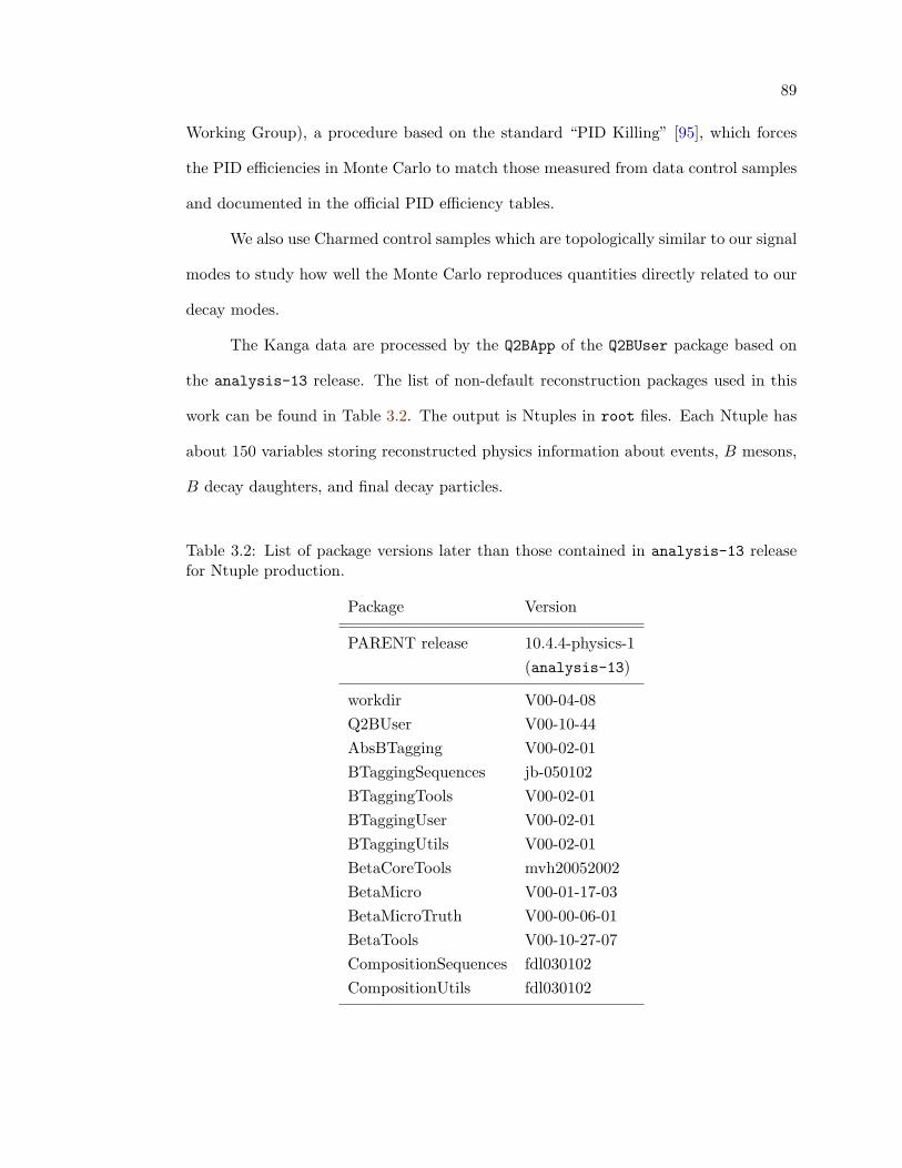
89

Working Group), a procedure based on the standard “PID Killing” [95], which forces

the PID efficiencies in Monte Carlo to match those measured from data control samples

and documented in the official PID efficiency tables.

We also use Charmed control samples which are topologically similar to our signal

modes to study how well the Monte Carlo reproduces quantities directly related to our

decay modes.

The Kanga data are processed by the Q2BApp of the Q2BUser package based on

the analysis-13 release. The list of non-default reconstruction packages used in this

work can be found in Table 3.2. The output is Ntuples in root files. Each Ntuple has

about 150 variables storing reconstructed physics information about events, B mesons,

B decay daughters, and final decay particles.

Table 3.2: List of package versions later than those contained in analysis-13 releasefor Ntuple production.

Package Version

PARENT release 10.4.4-physics-1(analysis-13)

workdir V00-04-08Q2BUser V00-10-44AbsBTagging V00-02-01BTaggingSequences jb-050102BTaggingTools V00-02-01BTaggingUser V00-02-01BTaggingUtils V00-02-01BetaCoreTools mvh20052002BetaMicro V00-01-17-03BetaMicroTruth V00-00-06-01BetaTools V00-10-27-07CompositionSequences fdl030102CompositionUtils fdl030102

90

3.3 Particle Reconstruction and Identification

The reconstructed data for physics analysis are candidate lists of charged tracks,

neutral particles as energy deposits in the EMC, etc. We use these candidates to re-

construct our final decay products, B daughter particles, B mesons, and event shape

variables.

3.3.1 Charged Tracks

Several charged track lists are defined for analysis purposes, including:

• ChargedTracks:

Candidates with non-zero charge and with pion mass hypothesis.

• GoodTracksVeryLoose: Subset of ChargedTracks with additional requirements:

∗ 0 < pT < 10 GeV/c;

∗ DOCAxy < 1.5 cm;∗

∗ |DOCAz| < 10 cm.

• GoodTracksLoose: Subset of GoodTracksVeryLoose with:

∗ pT > 0.1 GeV/c;

∗ DCH Hits ≥ 12.

• GoodTracksAccLoose: Subset of GoodTracksLoose with:

∗ 0.410 < θ < 2.54 rad.

• GoodTracksTight: Subset of GoodTracksLoose with additional cuts:

∗ DCH Hits ≥ 20.

∗ DOCAxy < 1 cm;

∗ |DOCAz| < 3 cm.

∗ DOCA: Distance of closest approach of a track to the beam spot center

91

We use ChargedTracks, GoodTracksVeryLoose, and GoodTracksLoose charged track

lists for our analyses.

3.3.2 Neutral Particles

Similar to charged tracks, the neutral particles reconstructed from the EMC are

organized in several lists:

• CalorNeutral: Candidates which are single EMC bumps not matched with any

track. Photon mass hypothesis assigned.

• CalorClusterNeutral: Candidates that are multi-bump neutral clusters or

single bumps which are not part of a cluster which is matched with a track.

• GoodNeutralLooseAcc: Subset of CalorNeutral with additional requirements:

∗ E > 30 MeV;

∗ Lateral Moment ≤ 1.1;

∗ 0.410 < θ < 2.409.

• GoodPhotonLoose: Subset of CalorNeutral with additional requirements:

∗ E > 30 MeV;

∗ Lateral Moment ≤ 0.8.

• GoodPhotonDefault: Subset of GoodPhotonLoose with:

∗ Eγ > 100 MeV;

We use GoodPhotonLoose list for photons in our analyses.

3.3.3 Electron, Muon, and Proton Identification

Electrons, muons, or protons are not in the final states of B decays in our studies

and we need to identify and reject these background tracks.

As we have discussed in Chapter 2, electrons are separated from charged hadrons

primarily on the basis of the shower energy, lateral shower moments, and track momen-

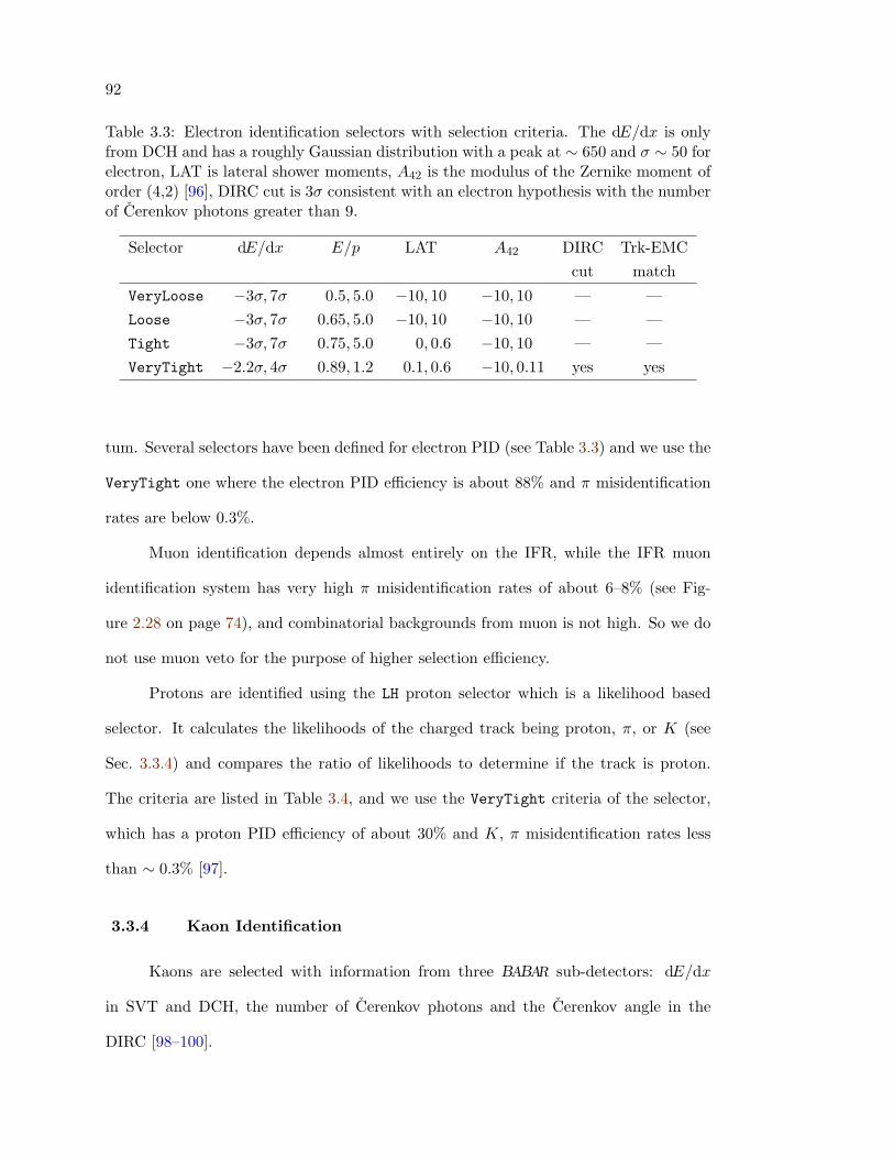
92

Table 3.3: Electron identification selectors with selection criteria. The dE/dx is onlyfrom DCH and has a roughly Gaussian distribution with a peak at ∼ 650 and σ ∼ 50 forelectron, LAT is lateral shower moments, A42 is the modulus of the Zernike moment oforder (4,2) [96], DIRC cut is 3σ consistent with an electron hypothesis with the numberof Cerenkov photons greater than 9.

Selector dE/dx E/p LAT A42 DIRC Trk-EMCcut match

VeryLoose −3σ, 7σ 0.5, 5.0 −10, 10 −10, 10 — —Loose −3σ, 7σ 0.65, 5.0 −10, 10 −10, 10 — —Tight −3σ, 7σ 0.75, 5.0 0, 0.6 −10, 10 — —VeryTight −2.2σ, 4σ 0.89, 1.2 0.1, 0.6 −10, 0.11 yes yes

tum. Several selectors have been defined for electron PID (see Table 3.3) and we use the

VeryTight one where the electron PID efficiency is about 88% and π misidentification

rates are below 0.3%.

Muon identification depends almost entirely on the IFR, while the IFR muon

identification system has very high π misidentification rates of about 6–8% (see Fig-

ure 2.28 on page 74), and combinatorial backgrounds from muon is not high. So we do

not use muon veto for the purpose of higher selection efficiency.

Protons are identified using the LH proton selector which is a likelihood based

selector. It calculates the likelihoods of the charged track being proton, π, or K (see

Sec. 3.3.4) and compares the ratio of likelihoods to determine if the track is proton.

The criteria are listed in Table 3.4, and we use the VeryTight criteria of the selector,

which has a proton PID efficiency of about 30% and K, π misidentification rates less

than ∼ 0.3% [97].

3.3.4 Kaon Identification

Kaons are selected with information from three BABAR sub-detectors: dE/dx

in SVT and DCH, the number of Cerenkov photons and the Cerenkov angle in the

DIRC [98–100].

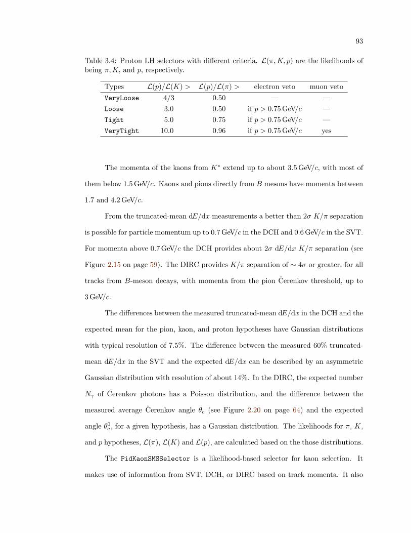
93

Table 3.4: Proton LH selectors with different criteria. L(π,K, p) are the likelihoods ofbeing π,K, and p, respectively.

Types L(p)/L(K) > L(p)/L(π) > electron veto muon veto

VeryLoose 4/3 0.50 — —Loose 3.0 0.50 if p > 0.75 GeV/c —Tight 5.0 0.75 if p > 0.75 GeV/c —VeryTight 10.0 0.96 if p > 0.75 GeV/c yes

The momenta of the kaons from K∗ extend up to about 3.5 GeV/c, with most of

them below 1.5 GeV/c. Kaons and pions directly from B mesons have momenta between

1.7 and 4.2 GeV/c.

From the truncated-mean dE/dx measurements a better than 2σ K/π separation

is possible for particle momentum up to 0.7 GeV/c in the DCH and 0.6 GeV/c in the SVT.

For momenta above 0.7GeV/c the DCH provides about 2σ dE/dx K/π separation (see

Figure 2.15 on page 59). The DIRC provides K/π separation of ∼ 4σ or greater, for all

tracks from B-meson decays, with momenta from the pion Cerenkov threshold, up to

3 GeV/c.

The differences between the measured truncated-mean dE/dx in the DCH and the

expected mean for the pion, kaon, and proton hypotheses have Gaussian distributions

with typical resolution of 7.5%. The difference between the measured 60% truncated-

mean dE/dx in the SVT and the expected dE/dx can be described by an asymmetric

Gaussian distribution with resolution of about 14%. In the DIRC, the expected number

Nγ of Cerenkov photons has a Poisson distribution, and the difference between the

measured average Cerenkov angle θc (see Figure 2.20 on page 64) and the expected

angle θ0c , for a given hypothesis, has a Gaussian distribution. The likelihoods for π, K,

and p hypotheses, L(π), L(K) and L(p), are calculated based on the those distributions.

The PidKaonSMSSelector is a likelihood-based selector for kaon selection. It

makes use of information from SVT, DCH, or DIRC based on track momenta. It also

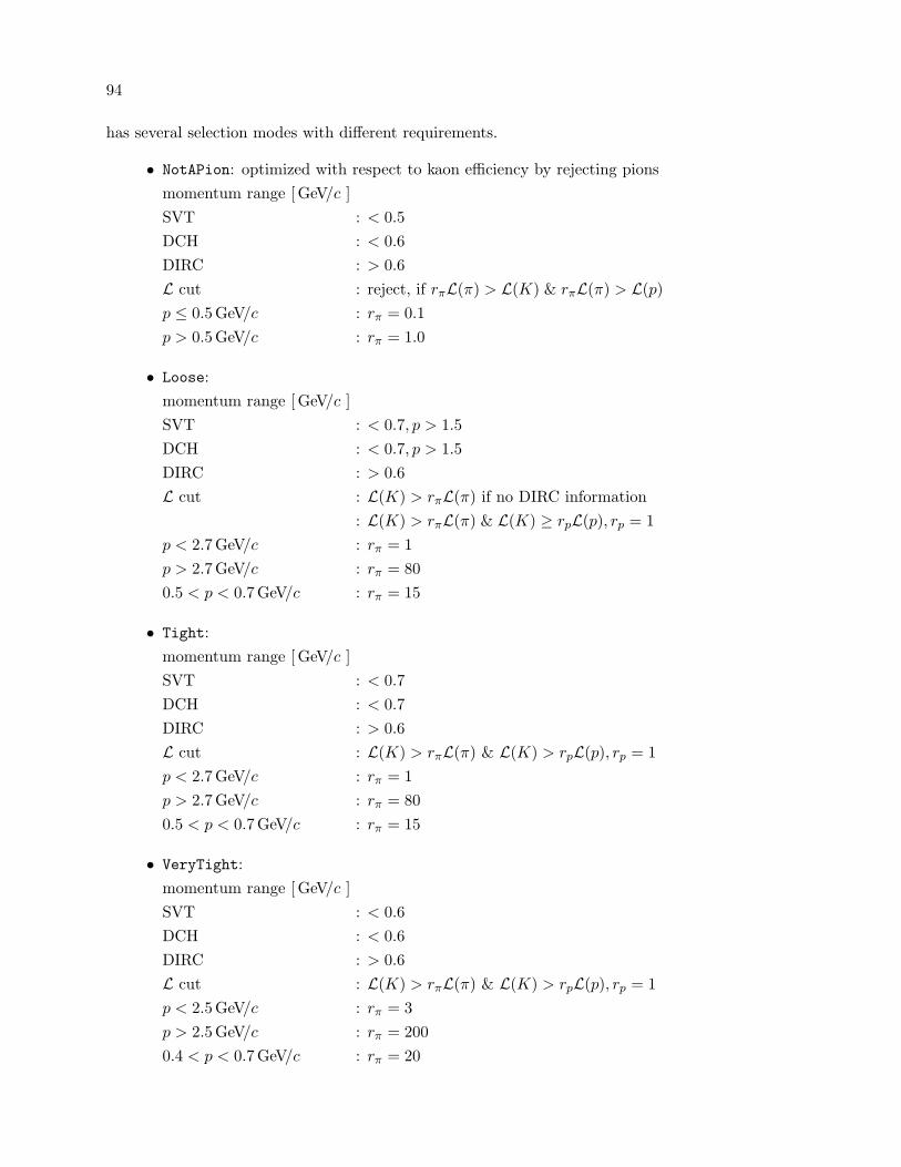
94

has several selection modes with different requirements.

• NotAPion: optimized with respect to kaon efficiency by rejecting pionsmomentum range [ GeV/c ]SVT : < 0.5DCH : < 0.6DIRC : > 0.6L cut : reject, if rπL(π) > L(K) & rπL(π) > L(p)p ≤ 0.5 GeV/c : rπ = 0.1p > 0.5 GeV/c : rπ = 1.0

• Loose:momentum range [ GeV/c ]SVT : < 0.7, p > 1.5DCH : < 0.7, p > 1.5DIRC : > 0.6L cut : L(K) > rπL(π) if no DIRC information

: L(K) > rπL(π) & L(K) ≥ rpL(p), rp = 1p < 2.7 GeV/c : rπ = 1p > 2.7 GeV/c : rπ = 800.5 < p < 0.7 GeV/c : rπ = 15

• Tight:momentum range [ GeV/c ]SVT : < 0.7DCH : < 0.7DIRC : > 0.6L cut : L(K) > rπL(π) & L(K) > rpL(p), rp = 1p < 2.7 GeV/c : rπ = 1p > 2.7 GeV/c : rπ = 800.5 < p < 0.7 GeV/c : rπ = 15

• VeryTight:momentum range [ GeV/c ]SVT : < 0.6DCH : < 0.6DIRC : > 0.6L cut : L(K) > rπL(π) & L(K) > rpL(p), rp = 1p < 2.5 GeV/c : rπ = 3p > 2.5 GeV/c : rπ = 2000.4 < p < 0.7 GeV/c : rπ = 20

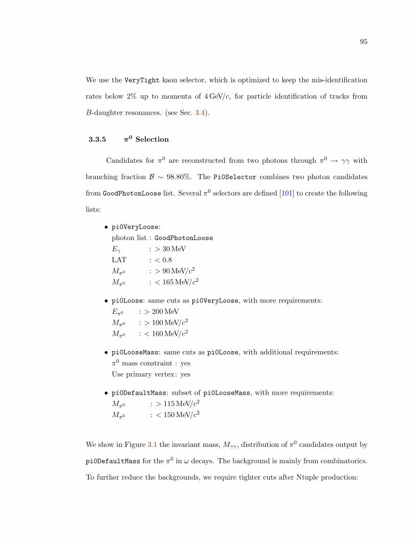
95

We use the VeryTight kaon selector, which is optimized to keep the mis-identification

rates below 2% up to momenta of 4 GeV/c, for particle identification of tracks from

B-daughter resonances. (see Sec. 3.4).

3.3.5 π0 Selection

Candidates for π0 are reconstructed from two photons through π0 → γγ with

branching fraction B ∼ 98.80%. The Pi0Selector combines two photon candidates

from GoodPhotonLoose list. Several π0 selectors are defined [101] to create the following

lists:

• pi0VeryLoose:photon list : GoodPhotonLooseEγ : > 30 MeVLAT : < 0.8Mπ0 : > 90 MeV/c2

Mπ0 : < 165 MeV/c2

• pi0Loose: same cuts as pi0VeryLoose, with more requirements:Eπ0 : > 200 MeVMπ0 : > 100 MeV/c2

Mπ0 : < 160 MeV/c2

• pi0LooseMass: same cuts as pi0Loose, with additional requirements:π0 mass constraint : yesUse primary vertex: yes

• pi0DefaultMass: subset of pi0LooseMass, with more requirements:Mπ0 : > 115 MeV/c2

Mπ0 : < 150 MeV/c2

We show in Figure 3.1 the invariant mass, Mγγ , distribution of π0 candidates output by

pi0DefaultMass for the π0 in ω decays. The background is mainly from combinatorics.

To further reduce the backgrounds, we require tighter cuts after Ntuple production:

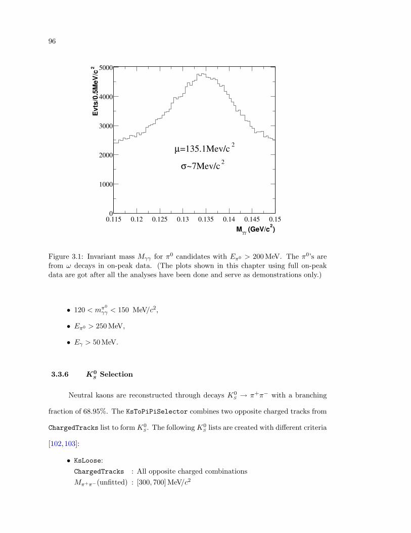
96

)2 (GeV/cγγM0.115 0.12 0.125 0.13 0.135 0.14 0.145 0.15

2E

vts/

0.5M

eV/c

0

1000

2000

3000

4000

5000

2~7Mev/cσ

2=135.1Mev/cµ

Figure 3.1: Invariant mass Mγγ for π0 candidates with Eπ0 > 200 MeV. The π0’s arefrom ω decays in on-peak data. (The plots shown in this chapter using full on-peakdata are got after all the analyses have been done and serve as demonstrations only.)

• 120 < mπ0

γγ < 150 MeV/c2,

• Eπ0 > 250 MeV,

• Eγ > 50 MeV.

3.3.6 K0S

Selection

Neutral kaons are reconstructed through decays K0S → π+π− with a branching

fraction of 68.95%. The KsToPiPiSelector combines two opposite charged tracks from

ChargedTracks list to formK0S . The followingK0

S lists are created with different criteria

[102,103]:

• KsLoose:ChargedTracks : All opposite charged combinationsMπ+π−(unfitted) : [300, 700]MeV/c2

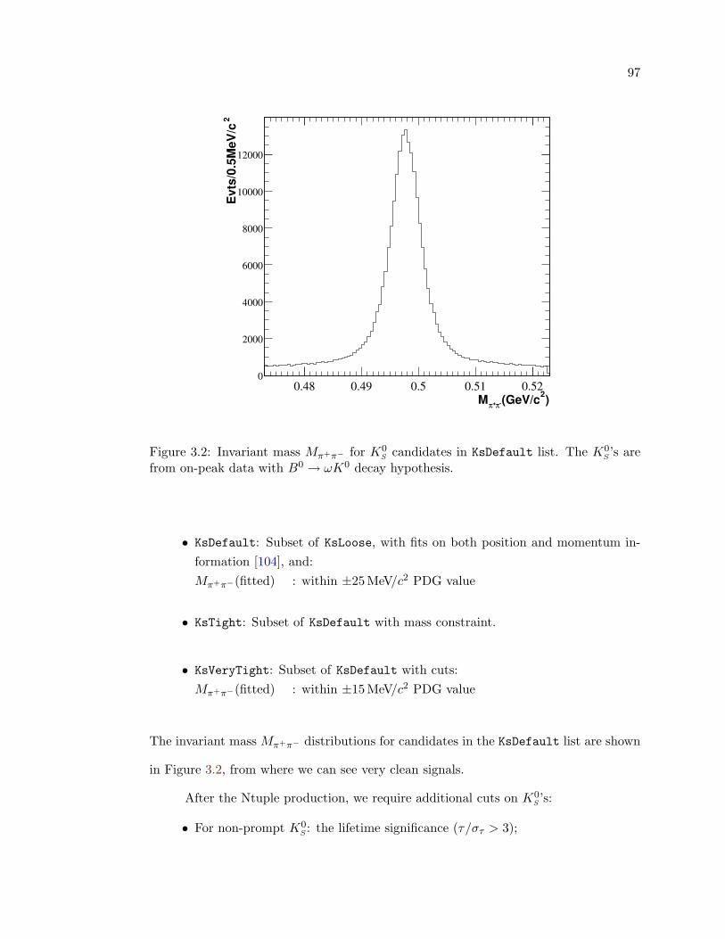
97

)2(GeV/c-π+πM0.48 0.49 0.5 0.51 0.52

2E

vts/

0.5M

eV/c

0

2000

4000

6000

8000

10000

12000

Figure 3.2: Invariant mass Mπ+π− for K0S candidates in KsDefault list. The K0

S ’s arefrom on-peak data with B0 → ωK0 decay hypothesis.

• KsDefault: Subset of KsLoose, with fits on both position and momentum in-formation [104], and:Mπ+π−(fitted) : within ±25 MeV/c2 PDG value

• KsTight: Subset of KsDefault with mass constraint.

• KsVeryTight: Subset of KsDefault with cuts:Mπ+π−(fitted) : within ±15 MeV/c2 PDG value

The invariant mass Mπ+π− distributions for candidates in the KsDefault list are shown

in Figure 3.2, from where we can see very clean signals.

After the Ntuple production, we require additional cuts on K0S ’s:

• For non-prompt K0S : the lifetime significance (τ/στ > 3);

98

• For prompt K0S :

∗ Primary vertex is used in the KsDefault selector,

∗ three-dimensional flight distance from the primary vertex > 2 mm,

∗ two-dimensional angle between flight and momentum vectors < 40 mrad.

We also set tighter mass range of K0S for both cases: 488 < M

K0S

ππ < 508 MeV/c2, but do

not apply any further PID cuts to its π+π− daughters.

3.4 B Daughter Selection

We will discuss the reconstruction and selection of B decay products in this

section. The distributions of the invariant masses of B daughters and other physics

quantities, which can be described by probability density functions (PDFs), are very

important to distinguish signals from backgrounds, and we rely on their discriminating

power to get final results.

3.4.1 ω Selection

The ω mesons are reconstructed from two charged tracks in GoodTracksLoose list

and a π0 in pi0DefaultMass list through the channel ω → π+π−π0 with a branching

fraction of 89.1%. After combining two charged tracks and one neutral track, the

ω selector does kinematic and geometric fits to the candidates and also requires the

invariant mass within a [−50, 50]MeV/c2 range of the ω mass [12]. We make additional

cuts after finishing the Beta job and require:

• 735 < mωπππ < 825 MeV/c2,

• Additional cuts on π0 as in Sec. 3.3.5,

• Charge π’s must NOT satisfy the VeryTight criteria of the electron Micro

selector, or the VeryTight criteria of the proton LH selector (see Sec. 3.3.3),

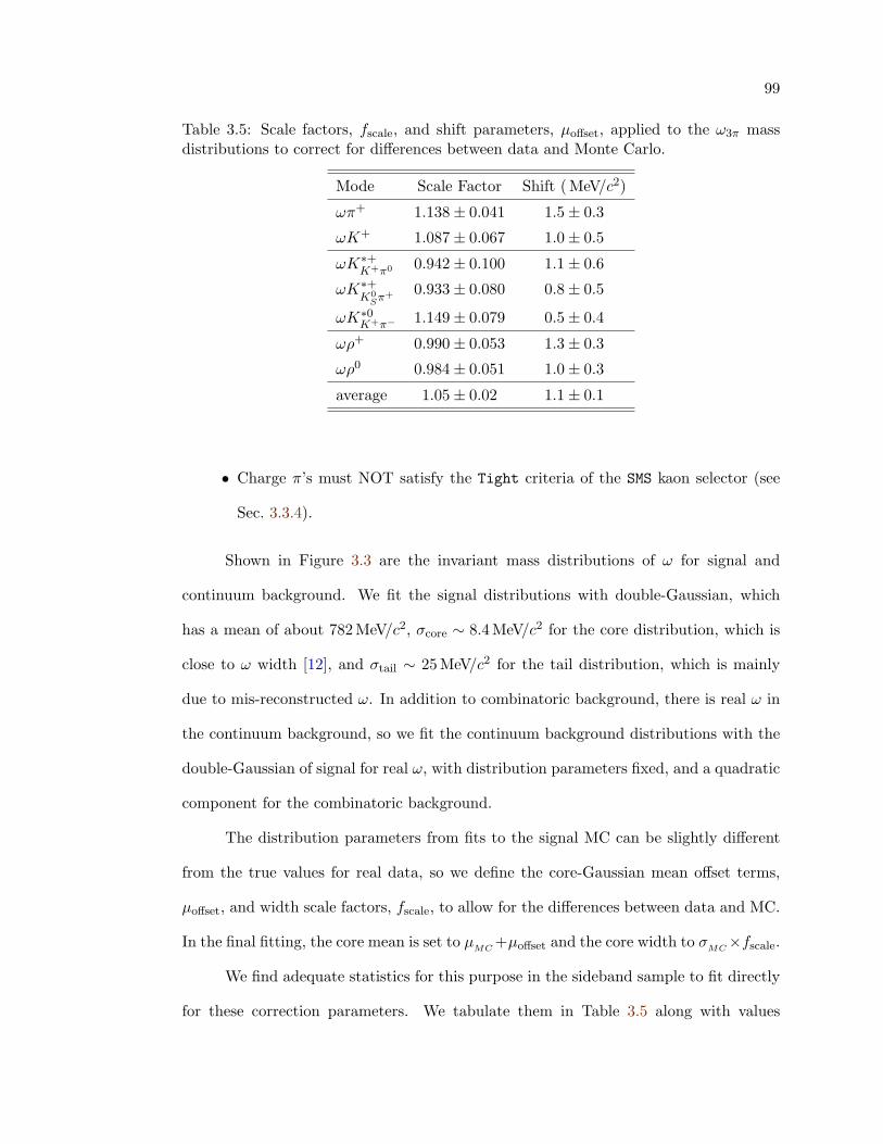
99

Table 3.5: Scale factors, fscale, and shift parameters, µoffset, applied to the ω3π massdistributions to correct for differences between data and Monte Carlo.

Mode Scale Factor Shift ( MeV/c2)

ωπ+ 1.138± 0.041 1.5± 0.3

ωK+ 1.087± 0.067 1.0± 0.5

ωK∗+K+π0 0.942± 0.100 1.1± 0.6

ωK∗+K0

Sπ+ 0.933± 0.080 0.8± 0.5

ωK∗0K+π− 1.149± 0.079 0.5± 0.4

ωρ+ 0.990± 0.053 1.3± 0.3

ωρ0 0.984± 0.051 1.0± 0.3

average 1.05± 0.02 1.1± 0.1

• Charge π’s must NOT satisfy the Tight criteria of the SMS kaon selector (see

Sec. 3.3.4).

Shown in Figure 3.3 are the invariant mass distributions of ω for signal and

continuum background. We fit the signal distributions with double-Gaussian, which

has a mean of about 782 MeV/c2, σcore ∼ 8.4 MeV/c2 for the core distribution, which is

close to ω width [12], and σtail ∼ 25 MeV/c2 for the tail distribution, which is mainly

due to mis-reconstructed ω. In addition to combinatoric background, there is real ω in

the continuum background, so we fit the continuum background distributions with the

double-Gaussian of signal for real ω, with distribution parameters fixed, and a quadratic

component for the combinatoric background.

The distribution parameters from fits to the signal MC can be slightly different

from the true values for real data, so we define the core-Gaussian mean offset terms,

µoffset, and width scale factors, fscale, to allow for the differences between data and MC.

In the final fitting, the core mean is set to µMC +µoffset and the core width to σMC×fscale.

We find adequate statistics for this purpose in the sideband sample to fit directly

for these correction parameters. We tabulate them in Table 3.5 along with values

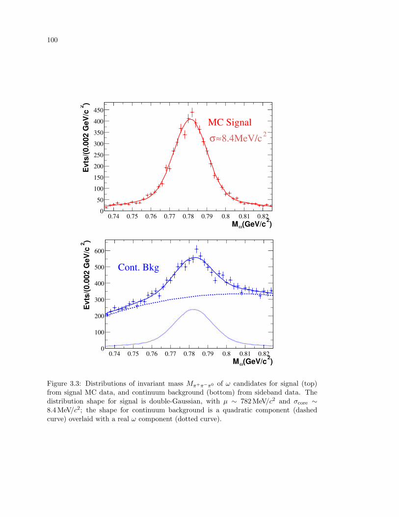
100

)2(GeV/cωM0.74 0.75 0.76 0.77 0.78 0.79 0.8 0.81 0.82

)2E

vts/

(0.0

02 G

eV/c

0

50

100

150

200

250

300

350

400

450

MC Signal28.4MeV/c≈σ

)2(GeV/cωM0.74 0.75 0.76 0.77 0.78 0.79 0.8 0.81 0.82

)2E

vts/

(0.0

02 G

eV/c

0

100

200

300

400

500

600

Cont. Bkg

Figure 3.3: Distributions of invariant mass Mπ+π−π0 of ω candidates for signal (top)from signal MC data, and continuum background (bottom) from sideband data. Thedistribution shape for signal is double-Gaussian, with µ ∼ 782 MeV/c2 and σcore ∼8.4 MeV/c2; the shape for continuum background is a quadratic component (dashedcurve) overlaid with a real ω component (dotted curve).

101

averaged over the several fits [105,106]. These averages become fixed parameters in the

final fits.

3.4.2 K/π Separation

As we have discussed in Sec. 2.3.3, and 3.3.4, the high momentum K/π tracks

directly from B mesons are identified mainly through information from DIRC. When

a high momentum charged track with β = v/c passes the DIRC, Cerenkov photons

are emitted to form a light cone in the particle flight direction with open angle θc, the

Cerenkov angle, being cos−1(1/nβ), where n = 1.473 is the index of refraction of the

DIRC quartz bar. The DIRC measures θc with an error of σθc , and for each particle

identification hypothesis, there is an expected Cerenkov angle, θci, where i = K,π. We

define the DIRC pull Si as:

Si =θc − θc

i

σθc

, i = K,π. (3.1)

The pull Si distributions for particle with correct hypotheses are normal Gaussian with

µ = 0, and σ = 1, while those for wrong hypotheses are shifted from zero, with wider

widths, as shown in Figure 3.4.

We include the pull distributions in our final fits for modes with a bachelor track

directly from B’s and fit the modes with K/π together, so we make very loose cuts on

the pulls after Beta jobs:

• −3.5 < SK < 24.5,

• −24.5 < Sπ < 3.5

and let the fitter resolve the ambiguity of K/π identification for the overlapped region

between the two distributions. We also require the number of measured Cerenkov

photons (DIRC PMT hits) for the bachelor track > 5 to ensure the quality of θc.

The DIRC pull calculation is done actually after Beta jobs and just before we

make additional cuts, using information of θc, θcK/π, track momentum, charge, etc.,

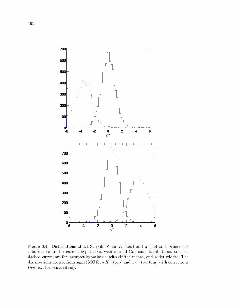
102

KS-6 -4 -2 0 2 4 60

100

200

300

400

500

600

700

πS-6 -4 -2 0 2 4 60

100

200

300

400

500

600

700

Figure 3.4: Distributions of DIRC pull Si for K (top) and π (bottom), where thesolid curves are for correct hypotheses, with normal Gaussian distributions, and thedashed curves are for incorrect hypotheses, with shifted means, and wider widths. Thedistributions are got from signal MC for ωK+ (top) and ωπ+ (bottom) with corrections(see text for explanation).

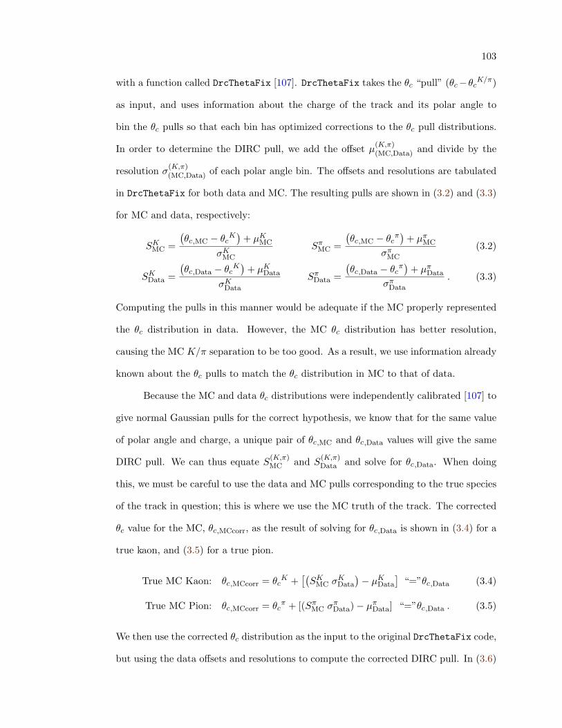
103

with a function called DrcThetaFix [107]. DrcThetaFix takes the θc “pull” (θc−θcK/π)

as input, and uses information about the charge of the track and its polar angle to

bin the θc pulls so that each bin has optimized corrections to the θc pull distributions.

In order to determine the DIRC pull, we add the offset µ(K,π)(MC,Data) and divide by the

resolution σ(K,π)(MC,Data) of each polar angle bin. The offsets and resolutions are tabulated

in DrcThetaFix for both data and MC. The resulting pulls are shown in (3.2) and (3.3)

for MC and data, respectively:

SKMC =

(θc,MC − θc

K)

+ µKMC

σKMC

SπMC =

(θc,MC − θc

π)

+ µπMC

σπMC

(3.2)

SKData =

(θc,Data − θc

K)

+ µKData

σKData

SπData =

(θc,Data − θc

π)

+ µπData

σπData

. (3.3)

Computing the pulls in this manner would be adequate if the MC properly represented

the θc distribution in data. However, the MC θc distribution has better resolution,

causing the MC K/π separation to be too good. As a result, we use information already

known about the θc pulls to match the θc distribution in MC to that of data.

Because the MC and data θc distributions were independently calibrated [107] to

give normal Gaussian pulls for the correct hypothesis, we know that for the same value

of polar angle and charge, a unique pair of θc,MC and θc,Data values will give the same

DIRC pull. We can thus equate S(K,π)MC and S

(K,π)Data and solve for θc,Data. When doing

this, we must be careful to use the data and MC pulls corresponding to the true species

of the track in question; this is where we use the MC truth of the track. The corrected

θc value for the MC, θc,MCcorr, as the result of solving for θc,Data is shown in (3.4) for a

true kaon, and (3.5) for a true pion.

True MC Kaon: θc,MCcorr = θcK +

[(SK

MC σKData

)− µK

Data

]“=”θc,Data (3.4)

True MC Pion: θc,MCcorr = θcπ + [(Sπ

MC σπData)− µπ

Data] “=”θc,Data . (3.5)

We then use the corrected θc distribution as the input to the original DrcThetaFix code,

but using the data offsets and resolutions to compute the corrected DIRC pull. In (3.6)

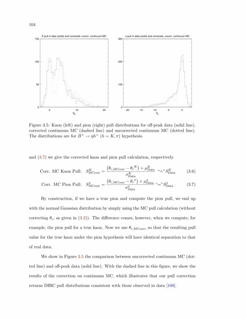
104

K pull in data (solid) and corrected, uncorr. continuum MC

0 10 20SK

0

50

100

150π pull in data (solid) and corrected, uncorr. continuum MC

-20 -15 -10 -5 0Sπ

0

100

200

300

Figure 3.5: Kaon (left) and pion (right) pull distributions for off-peak data (solid line),corrected continuum MC (dashed line) and uncorrected continuum MC (dotted line).The distributions are for B+ → ηh+ (h = K,π) hypothesis.

and (3.7) we give the corrected kaon and pion pull calculation, respectively.

Corr. MC Kaon Pull: SKMCcorr =

(θc,MCcorr − θc

K)

+ µKData

σKData

“=”SKData (3.6)

Corr. MC Pion Pull: SπMCcorr =

(θc,MCcorr − θc

π)

+ µπData

σπData

“=”SπData . (3.7)

By construction, if we have a true pion and compute the pion pull, we end up

with the normal Gaussian distribution by simply using the MC pull calculation (without

correcting θc, as given in (3.2)). The difference comes, however, when we compute, for

example, the pion pull for a true kaon. Now we use θc,MCcorr, so that the resulting pull

value for the true kaon under the pion hypothesis will have identical separation to that

of real data.

We show in Figure 3.5 the comparison between uncorrected continuum MC (dot-

ted line) and off-peak data (solid line). With the dashed line in this figure, we show the

results of the correction on continuum MC, which illustrates that our pull correction

returns DIRC pull distributions consistent with those observed in data [108].

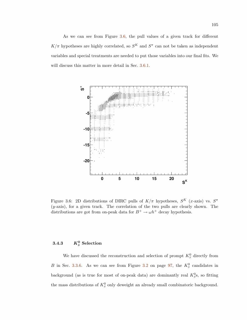
105

As we can see from Figure 3.6, the pull values of a given track for different

K/π hypotheses are highly correlated, so SK and Sπ can not be taken as independent

variables and special treatments are needed to put those variables into our final fits. We

will discuss this matter in more detail in Sec. 3.6.1.

KS0 5 10 15 20

πS

-20

-15

-10

-5

0

Figure 3.6: 2D distributions of DIRC pulls of K/π hypotheses, SK (x-axis) vs. Sπ

(y-axis), for a given track. The correlation of the two pulls are clearly shown. Thedistributions are got from on-peak data for B+ → ωh+ decay hypothesis.

3.4.3 K0S

Selection

We have discussed the reconstruction and selection of prompt K0S directly from

B in Sec. 3.3.6. As we can see from Figure 3.2 on page 97, the K0S candidates in

background (as is true for most of on-peak data) are dominantly real K0Ss, so fitting

the mass distributions of K0S only deweight an already small combinatoric background.

106

Thus we only apply the cuts listed in Sec. 3.3.6 to K0S in the Ntuples and do not include

K0S masses in our final fits.

3.4.4 K∗ Selection

We reconstruct K∗+ from two channels: K∗+ → K0Sπ

+ and K∗+ → K+π0,

both with branching fractions of 33.3%, and K∗0 from K∗0 → K+π− with a branching

fraction of 66.7%.

One charged track from GoodTracksLoose list of π hypothesis and one K0S from

KsDefault list are combined to form K∗+ candidates, or K∗+ are selected from com-

binations of one charged track from GoodTracksLoose with K hypothesis and one π0

from pi0DefaultMass list. Two opposite charged tracks from GoodTracksLoose are

combined to form K∗0 candidates. The selectors require the invariant masses of K+π−

andK0Sπ

+ to be within [−100, 100]MeV/c2 range of the known value [12] of the K∗ mass,

and K+π0 combinations within [−150, 150] MeV/c2 range. The selectors do vertex fits

on the candidates using both kinematic and geometric information. Combinations with

good fit quality are stored in candidate lists KstarKsPiLoose, KstarKPi0Loose, and

KstarKPiLoose, for K∗+K0

Sπ+ , K∗+K+π0 , and K∗0

K+π− candidates, respectively, for recon-

struction of B mesons.

We make additional cuts on the K∗ candidates after the Beta jobs have been

finished:

• 755 < mK∗Kπ < 1035 MeV/c2,

• Additional π0 cuts are made for modes with π0 (see Sec. 3.3.5 on page 95), but

without any cut on π0 energy. To reject soft π0s, we use decay angle cuts (see

Sec. 3.4.6.2),

• K0S ’s lifetime significance τ/στ > 3 for mode with K0

S ,

• Charged K’s or π’s must NOT satisfy the VeryTight criteria of the electron

Micro selector, or the VeryTight criteria of the proton LH selector (see Sec. 3.3.3),

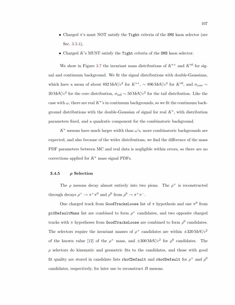
107

• Charged π’s must NOT satisfy the Tight criteria of the SMS kaon selector (see

Sec. 3.3.4),

• Charged K’s MUST satisfy the Tight criteria of the SMS kaon selector.

We show in Figure 3.7 the invariant mass distributions of K∗+ and K∗0 for sig-

nal and continuum background. We fit the signal distributions with double-Gaussians,

which have a mean of about 892 MeV/c2 for K∗+, ∼ 896 MeV/c2 for K∗0, and σcore ∼

20 MeV/c2 for the core distribution, σtail ∼ 50 MeV/c2 for the tail distribution. Like the

case with ω, there are realK∗’s in continuum backgrounds, so we fit the continuum back-

ground distributions with the double-Gaussian of signal for real K∗, with distribution

parameters fixed, and a quadratic component for the combinatoric background.

K∗ mesons have much larger width than ω’s, more combinatoric backgrounds are

expected, and also because of the wider distributions, we find the difference of the mass

PDF parameters between MC and real data is negligible within errors, so there are no

corrections applied for K∗ mass signal PDFs.

3.4.5 ρ Selection

The ρ mesons decay almost entirely into two pions. The ρ+ is reconstructed

through decays ρ+ → π+π0 and ρ0 from ρ0 → π+π−.

One charged track from GoodTracksLoose list of π hypothesis and one π0 from

pi0DefaultMass list are combined to form ρ+ candidates, and two opposite charged

tracks with π hypotheses from GoodTracksLoose are combined to form ρ0 candidates.

The selectors require the invariant masses of ρ+ candidates are within ±320 MeV/c2

of the known value [12] of the ρ+ mass, and ±300 MeV/c2 for ρ0 candidates. The

ρ selectors do kinematic and geometric fits to the candidates, and those with good

fit quality are stored in candidate lists rhoCDefault and rho0Default for ρ+ and ρ0

candidates, respectively, for later use to reconstruct B mesons.

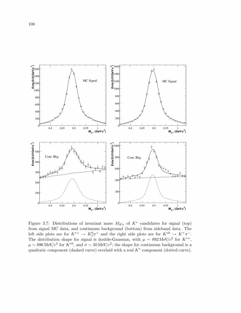
108

)2 (GeV/c+K*M0.8 0.85 0.9 0.95 1

)2E

vts/

(0.0

1GeV

/c

0

200

400

600

800

1000

1200

1400

1600

MC Signal

)2 (GeV/c0K*M

0.8 0.85 0.9 0.95 1

)2E

vts/

(0.0

1GeV

/c

0

200

400

600

800

1000

1200

1400

1600

MC Signal

)2 (GeV/c+K*M0.8 0.85 0.9 0.95 1

)2E

vts/

(0.0

1GeV

/c

0

100

200

300

400

500

Cont. Bkg

)2 (GeV/c0K*M

0.8 0.85 0.9 0.95 1

)2E

vts/

(0.0

1GeV

/c

0

200

400

600

800

1000

Cont. Bkg

Figure 3.7: Distributions of invariant mass MKπ of K∗ candidates for signal (top)from signal MC data, and continuum background (bottom) from sideband data. Theleft side plots are for K∗+ → K0

Sπ+ and the right side plots are for K∗0 → K+π−.

The distribution shape for signal is double-Gaussian, with µ ∼ 892 MeV/c2 for K∗+,µ ∼ 896 MeV/c2 for K∗0, and σ ∼ 50 MeV/c2; the shape for continuum background is aquadratic component (dashed curve) overlaid with a real K∗ component (dotted curve).

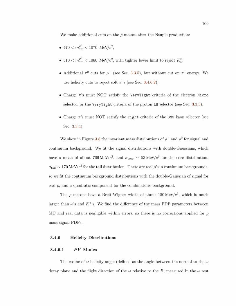
109

We make additional cuts on the ρ masses after the Ntuple production:

• 470 < mρ+

ππ < 1070 MeV/c2,

• 510 < mρ0

ππ < 1060 MeV/c2, with tighter lower limit to reject K0S ,

• Additional π0 cuts for ρ+ (see Sec. 3.3.5), but without cut on π0 energy. We

use helicity cuts to reject soft π0s (see Sec. 3.4.6.2),

• Charge π’s must NOT satisfy the VeryTight criteria of the electron Micro

selector, or the VeryTight criteria of the proton LH selector (see Sec. 3.3.3),

• Charge π’s must NOT satisfy the Tight criteria of the SMS kaon selector (see

Sec. 3.3.4),

We show in Figure 3.8 the invariant mass distributions of ρ+ and ρ0 for signal and

continuum background. We fit the signal distributions with double-Gaussians, which

have a mean of about 766 MeV/c2, and σcore ∼ 53 MeV/c2 for the core distribution,

σtail ∼ 170 MeV/c2 for the tail distribution. There are real ρ’s in continuum backgrounds,

so we fit the continuum background distributions with the double-Gaussian of signal for

real ρ, and a quadratic component for the combinatoric background.

The ρ mesons have a Breit-Wigner width of about 150 MeV/c2, which is much

larger than ω’s and K∗’s. We find the difference of the mass PDF parameters between

MC and real data is negligible within errors, so there is no corrections applied for ρ

mass signal PDFs.

3.4.6 Helicity Distributions

3.4.6.1 PV Modes

The cosine of ω helicity angle (defined as the angle between the normal to the ω

decay plane and the flight direction of the ω relative to the B, measured in the ω rest

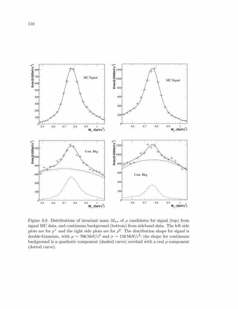
110

)2

(GeV/c+ρM0.5 0.6 0.7 0.8 0.9 1

)2E

vts/

(0.0

3GeV

/c

0

100

200

300

400

500

600

700

800

MC Signal

)2 (GeV/c0ρM

0.6 0.7 0.8 0.9 1

)2E

vts/

(0.0

29G

eV/c

0

200

400

600

800

1000

1200

MC Signal

)2

(GeV/c+ρM0.5 0.6 0.7 0.8 0.9 1

)2E

vts/

(0.0

3GeV

/c

0

200

400

600

800

1000

1200Cont. Bkg

)2 (GeV/c0ρM

0.6 0.7 0.8 0.9 1

)2E

vts/

(0.0

29G

eV/c

0

200

400

600

800

1000

1200

Cont. Bkg

Figure 3.8: Distributions of invariant mass Mππ of ρ candidates for signal (top) fromsignal MC data, and continuum background (bottom) from sideband data. The left sideplots are for ρ+ and the right side plots are for ρ0. The distribution shape for signal isdouble-Gaussian, with µ ∼ 766 MeV/c2 and σ ∼ 150 MeV/c2; the shape for continuumbackground is a quadratic component (dashed curve) overlaid with a real ρ component(dotted curve).

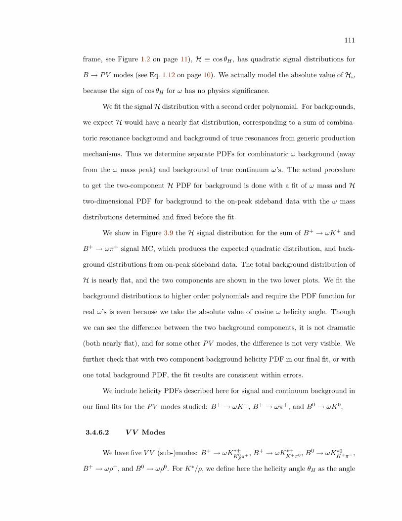
111

frame, see Figure 1.2 on page 11), H ≡ cos θH , has quadratic signal distributions for

B → PV modes (see Eq. 1.12 on page 10). We actually model the absolute value of Hω

because the sign of cos θH for ω has no physics significance.

We fit the signalH distribution with a second order polynomial. For backgrounds,

we expect H would have a nearly flat distribution, corresponding to a sum of combina-

toric resonance background and background of true resonances from generic production

mechanisms. Thus we determine separate PDFs for combinatoric ω background (away

from the ω mass peak) and background of true continuum ω’s. The actual procedure

to get the two-component H PDF for background is done with a fit of ω mass and H

two-dimensional PDF for background to the on-peak sideband data with the ω mass

distributions determined and fixed before the fit.

We show in Figure 3.9 the H signal distribution for the sum of B+ → ωK+ and

B+ → ωπ+ signal MC, which produces the expected quadratic distribution, and back-

ground distributions from on-peak sideband data. The total background distribution of

H is nearly flat, and the two components are shown in the two lower plots. We fit the

background distributions to higher order polynomials and require the PDF function for

real ω’s is even because we take the absolute value of cosine ω helicity angle. Though

we can see the difference between the two background components, it is not dramatic

(both nearly flat), and for some other PV modes, the difference is not very visible. We

further check that with two component background helicity PDF in our final fit, or with

one total background PDF, the fit results are consistent within errors.

We include helicity PDFs described here for signal and continuum background in

our final fits for the PV modes studied: B+ → ωK+, B+ → ωπ+, and B0 → ωK0.

3.4.6.2 V V Modes

We have five V V (sub-)modes: B+ → ωK∗+K0

Sπ+ , B+ → ωK∗+K+π0 , B0 → ωK∗0

K+π− ,

B+ → ωρ+, and B0 → ωρ0. For K∗/ρ, we define here the helicity angle θH as the angle

112

ωH0 0.1 0.2 0.3 0.4 0.5 0.6 0.7 0.8 0.9 1

Evt

s/(0

.02)

0

200

400

600

800

1000 MC Signal

flat≈Cont. Bkg

2 H∝

ωH0 0.1 0.2 0.3 0.4 0.5 0.6 0.7 0.8 0.9 1

Evt

s/0.

02

0

50

100

150

200

250

sideband bkgω

ωH0 0.1 0.2 0.3 0.4 0.5 0.6 0.7 0.8 0.9 1

Evt

s/0.

02

0

50

100

150

200

250

300

350

400

sideband subtracted bkgω

Figure 3.9: Distributions of cosine ω helicity angles for B → PV modes as in B+ →ωh+ decays. The top plots show the signal MC distributions fitted to a second orderpolynomial, and the total background distribution which is nearly flat. Two lowertwo plots show the two components of the background PDF. The left plot shows thedistribution of ω mass sideband for pure combinatorial background; the right plot showthe distribution of ω mass sideband subtracted background for real ω’s.

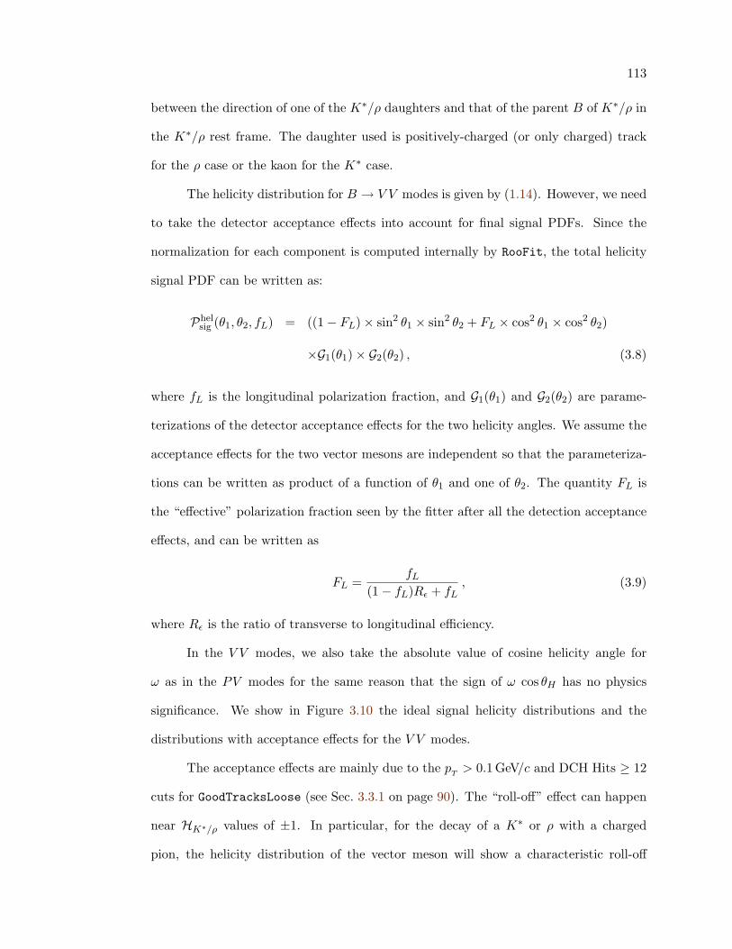
113

between the direction of one of the K∗/ρ daughters and that of the parent B of K∗/ρ in

the K∗/ρ rest frame. The daughter used is positively-charged (or only charged) track

for the ρ case or the kaon for the K∗ case.

The helicity distribution for B → V V modes is given by (1.14). However, we need

to take the detector acceptance effects into account for final signal PDFs. Since the

normalization for each component is computed internally by RooFit, the total helicity

signal PDF can be written as:

Phelsig (θ1, θ2, fL) = ((1− FL)× sin2 θ1 × sin2 θ2 + FL × cos2 θ1 × cos2 θ2)

×G1(θ1)× G2(θ2) , (3.8)

where fL is the longitudinal polarization fraction, and G1(θ1) and G2(θ2) are parame-

terizations of the detector acceptance effects for the two helicity angles. We assume the

acceptance effects for the two vector mesons are independent so that the parameteriza-

tions can be written as product of a function of θ1 and one of θ2. The quantity FL is

the “effective” polarization fraction seen by the fitter after all the detection acceptance

effects, and can be written as

FL =fL

(1− fL)Rε + fL, (3.9)

where Rε is the ratio of transverse to longitudinal efficiency.

In the V V modes, we also take the absolute value of cosine helicity angle for

ω as in the PV modes for the same reason that the sign of ω cos θH has no physics

significance. We show in Figure 3.10 the ideal signal helicity distributions and the

distributions with acceptance effects for the V V modes.

The acceptance effects are mainly due to the pT > 0.1 GeV/c and DCH Hits ≥ 12

cuts for GoodTracksLoose (see Sec. 3.3.1 on page 90). The “roll-off” effect can happen

near HK∗/ρ values of ±1. In particular, for the decay of a K∗ or ρ with a charged

pion, the helicity distribution of the vector meson will show a characteristic roll-off

114

ωH0 0.2 0.4 0.6 0.8 1ρ

K*/

H

-1-0.5

00.5

102468

101214

ωH0 0.2 0.4 0.6 0.8 1ρ

K*/

H

-1-0.5

00.5

10

2

4

6

8

10

12

Figure 3.10: The 2D signal H distributions for P → V V decays with perfect acceptance(left) and real acceptance effects (right), with the polarization fraction fL =0.5. The leftplot is got using distribution (1.14); the right plot is got using (3.8) with parametersof G1(θ1) and G2(θ2) determined from fits to B → ωρ signal MC with fL =0.5. Forcomparison purpose, the distributions are plotted over the full ranges of H. Due toacceptance effects, we have to make cuts on HK∗/ρ, so the actual ranges of H for K∗/ρin the final fits are narrower. See text for more detail.

in the region populated by low momentum pions because of the cuts on the pions by

the selector (see Figure 3.11). This effect is also present for low momentum charged

kaons but is negligible due to the shifted momentum fraction distribution of the strange

quarks. Those stringent quality requirements to the GoodTracksLoose list, however, are

necessary to reduce combinatorial background under the broad K∗ and ρ resonances.

The ω mesons can also have such soft pions, but the H angle is defined differently here

as the angle between the ω flight direction and the normal to the ω decay plane (see

Figure1.2 on page 11), so the soft pions dominate around H =0. For the Hω distribution

of the longitudinal component, the effects are invisible because of the quadratic nature

of the distribution, and for the transverse component, the effects are less severe because

the decay plane is less sensitive to the soft pions, as we show also in Figure 3.11, the ω

helicity distributions for longitudinal and transverse components.

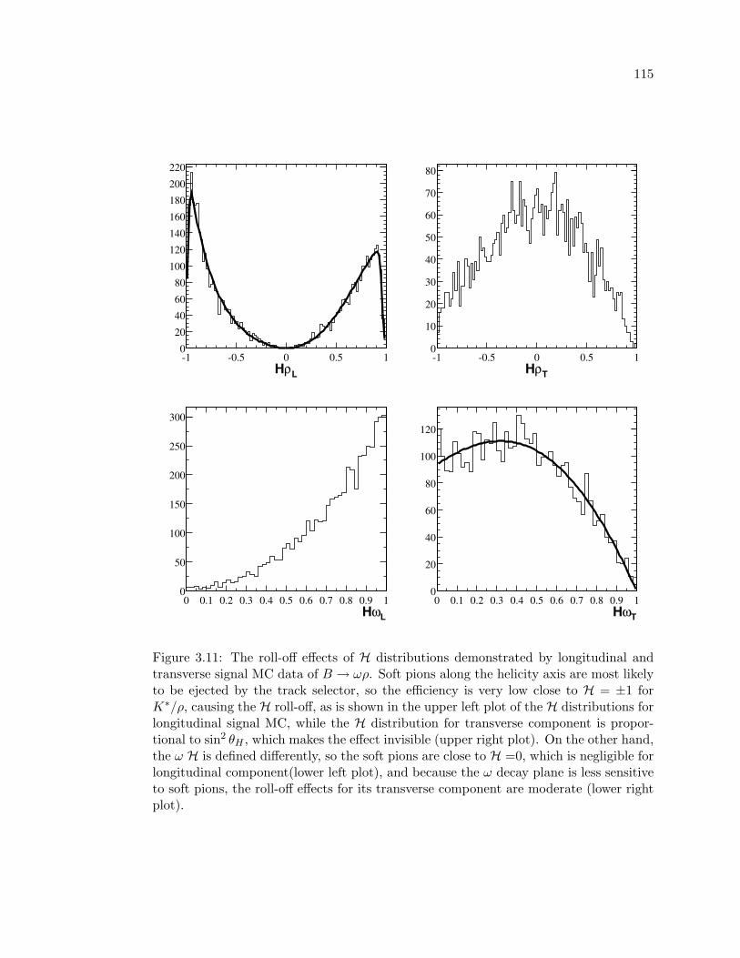
115

LρH-1 -0.5 0 0.5 10

20

40

60

80

100

120

140

160

180

200

220

TρH-1 -0.5 0 0.5 10

10

20

30

40

50

60

70

80

LωH0 0.1 0.2 0.3 0.4 0.5 0.6 0.7 0.8 0.9 1

0

50

100

150

200

250

300

TωH0 0.1 0.2 0.3 0.4 0.5 0.6 0.7 0.8 0.9 1

0

20

40

60

80

100

120

Figure 3.11: The roll-off effects of H distributions demonstrated by longitudinal andtransverse signal MC data of B → ωρ. Soft pions along the helicity axis are most likelyto be ejected by the track selector, so the efficiency is very low close to H = ±1 forK∗/ρ, causing the H roll-off, as is shown in the upper left plot of the H distributions forlongitudinal signal MC, while the H distribution for transverse component is propor-tional to sin2 θH , which makes the effect invisible (upper right plot). On the other hand,the ω H is defined differently, so the soft pions are close to H =0, which is negligible forlongitudinal component(lower left plot), and because the ω decay plane is less sensitiveto soft pions, the roll-off effects for its transverse component are moderate (lower rightplot).

116

The roll-off effects in the signal or background can be modeled by multiplying the

primary PDF shape by an appropriate Fermi function, which can be written as

GF (H;µthres, σslope) =1

1 + e±(H−µthres)/σslope, (3.10)

where µthres describes the position of the roll-off, σslope determines the sharpness of the

roll-off, and depending on the direction of roll-off, there is ‘+’ sign for the right-side

roll-off and ‘−’ sign for the left one.

Another source of acceptance effects is due to soft π0s for modes decaying to π0,

K∗+K+π0 and ρ+. Soft π0s are mainly background and we usually require energy cut to

get rid of soft π0s. For K∗+K+π0 or ρ+, the soft π0s are concentrating at H = −1 by

definition. We could cut on π0 energy, which has been done to π0s from ω, but we

prefer to cut directly on H so that we can directly get rid of the low acceptance range

of H due to soft π0 cuts. Requirement of H > −0.5 is effectively to have π0 energy cut

of > 350 MeV. To be conservative, we require H > −0.6 for these two modes.

It is inevitable either to model the acceptance effects, or to have cuts to remove

those low acceptance ranges. We choose a combined method. We reject those ranges as

much as possible to eliminate the uncertainty in modeling them, and also keep as much

as possible not to have the selection efficiency too low.

We list the cuts we apply to the H in Table 3.6. We choose the (±)0.85 K∗/ρ

helicity fiducial cut to remove as much as possible the region where the efficiency rolls

off. The efficiency loss from this is < 10% for longitudinal component which is more

sensitive to this cut. For modes with π0s, we need tighter cut, −0.6, to reject soft π0s.

Unlike some other V V modes, for example, ρρ, this cut will not lose as much efficiency

because there is only one such π0.

The residual acceptance effects are parameterized by G1(θ1) and G2(θ2) as high

order polynomials (up to seventh order) and/or the “roll-off” functions. We fit the total

PDF as in (3.8) to a cocktail of longitudinal and transverse signal MC data, the fL and

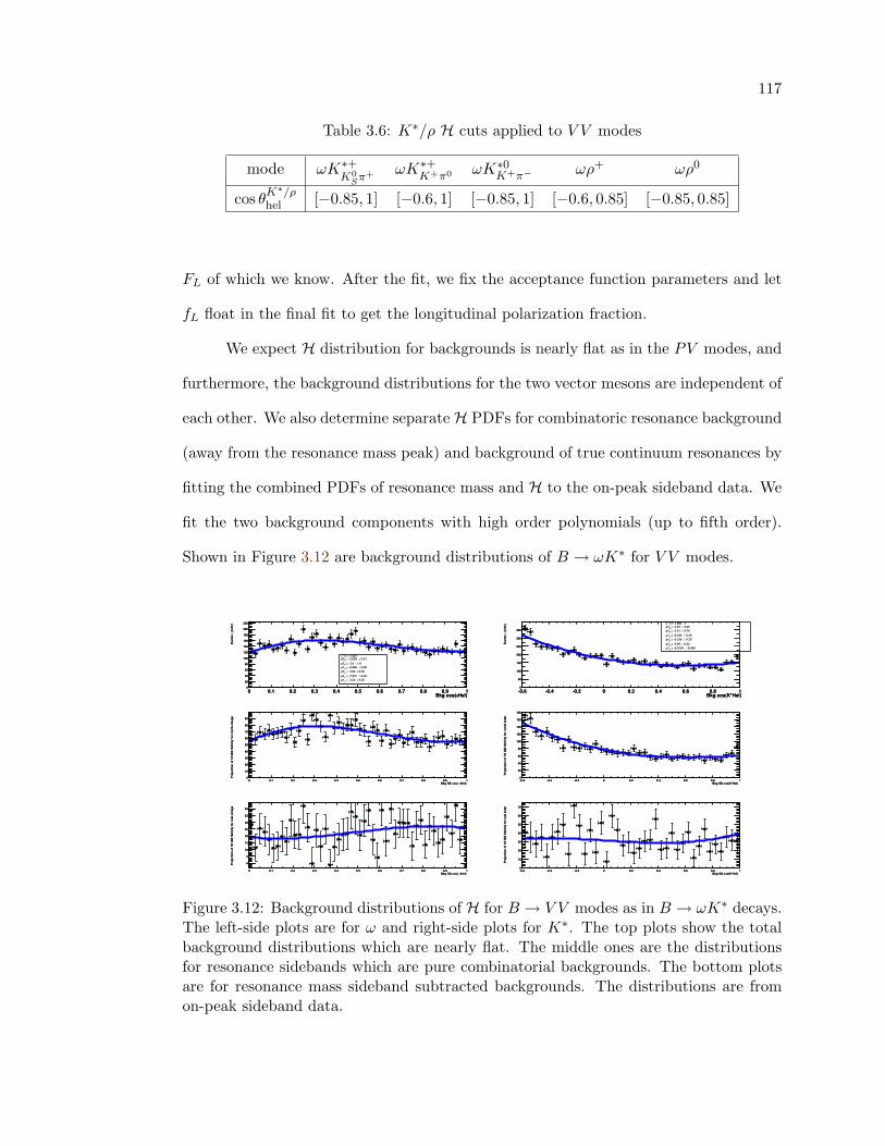
117

Table 3.6: K∗/ρ H cuts applied to V V modes

mode ωK∗+K0

Sπ+ ωK∗+K+π0 ωK∗0

K+π− ωρ+ ωρ0

cos θK∗/ρhel [−0.85, 1] [−0.6, 1] [−0.85, 1] [−0.6, 0.85] [−0.85, 0.85]

FL of which we know. After the fit, we fix the acceptance function parameters and let

fL float in the final fit to get the longitudinal polarization fraction.

We expect H distribution for backgrounds is nearly flat as in the PV modes, and

furthermore, the background distributions for the two vector mesons are independent of

each other. We also determine separate H PDFs for combinatoric resonance background

(away from the resonance mass peak) and background of true continuum resonances by

fitting the combined PDFs of resonance mass and H to the on-peak sideband data. We

fit the two background components with high order polynomials (up to fifth order).

Shown in Figure 3.12 are background distributions of B → ωK∗ for V V modes.

Hel)ωBkg cos(0 0.1 0.2 0.3 0.4 0.5 0.6 0.7 0.8 0.9 1

Eve

nts

/ ( 0

.02

)

0

20

40

60

80

100

120

140

160

180

200

220

0.24± = 3.23 Cp1 0.40± = -7.031 Cp2

0.30± = 3.82 Cp3 0.80± = -0.866 Rp1

1.0± = 3.8 Rp2 0.91± = -2.602 Rp3

/n = 1.5572χ

Hel)ωBkg cos(0 0.1 0.2 0.3 0.4 0.5 0.6 0.7 0.8 0.9 1

Eve

nts

/ ( 0

.02

)

0

20

40

60

80

100

120

140

160

180

200

220

Bkg cos(K*Hel)-0.6 -0.4 -0.2 0 0.2 0.4 0.6 0.8 1

Eve

nts

/ ( 0

.04

)

0

50

100

150

200

250

300

350

0.080± = -0.9754 Cp1 0.22± = 0.99 Cp2

0.25± = -0.226 Cp3 0.30± = -0.294 Rp1

0.70± = 0.01 Rp2 0.85± = 0.53 Rp3

/n = 1.8522

χ

Bkg cos(K*Hel)-0.6 -0.4 -0.2 0 0.2 0.4 0.6 0.8 1

Eve

nts

/ ( 0

.04

)

0

50

100

150

200

250

300

350

Hel)ωBkg SB cos(0 0.1 0.2 0.3 0.4 0.5 0.6 0.7 0.8 0.9 1

Pro

ject

ion

of 1

D Q

Q H

elic

ity fo

r co

mb

omeg

a

0

10

20

30

40

50

60

70

80

90

Hel)ωBkg SB cos(0 0.1 0.2 0.3 0.4 0.5 0.6 0.7 0.8 0.9 1

Pro

ject

ion

of 1

D Q

Q H

elic

ity fo

r co

mb

omeg

a

0

10

20

30

40

50

60

70

80

90

Bkg SB cos(K*Hel)-0.6 -0.4 -0.2 0 0.2 0.4 0.6 0.8 1

Pro

ject

ion

of 1

D Q

Q H

elic

ity fo

r co

mb

ksta

r

0

20

40

60

80

100

120

140

160

180

Bkg SB cos(K*Hel)-0.6 -0.4 -0.2 0 0.2 0.4 0.6 0.8 1

Pro

ject

ion

of 1

D Q

Q H

elic

ity fo

r co

mb

ksta

r

0

20

40

60

80

100

120

140

160

180

Hel)ωBkg SG cos(0 0.1 0.2 0.3 0.4 0.5 0.6 0.7 0.8 0.9 1

Pro

ject

ion

of 1

D Q

Q H

elic

ity fo

r re

al o

meg

a

0

5

10

15

20

25

30

35

40

Hel)ωBkg SG cos(0 0.1 0.2 0.3 0.4 0.5 0.6 0.7 0.8 0.9 1

Pro

ject

ion

of 1

D Q

Q H

elic

ity fo

r re

al o

meg

a

0

5

10

15

20

25

30

35

40

Bkg SG cos(K*Hel)-0.6 -0.4 -0.2 0 0.2 0.4 0.6 0.8 1

Pro

ject

ion

of 1

D Q

Q H

elic

ity fo

r re

al k

star

0

10

20

30

40

50

60

70

Bkg SG cos(K*Hel)-0.6 -0.4 -0.2 0 0.2 0.4 0.6 0.8 1

Pro

ject

ion

of 1

D Q

Q H

elic

ity fo

r re

al k

star

0

10

20

30

40

50

60

70

Hel)ωFeed cos(0 0.1 0.2 0.3 0.4 0.5 0.6 0.7 0.8 0.9 1

Eve

nts

/ ( 0

.02

)

0

2

4

6

8

10

12

5.9± = 1.6 Cp1 11± = 11 Cp2

7.7± = -12.33 Cp3/n = 0.4182χ

Hel)ωFeed cos(0 0.1 0.2 0.3 0.4 0.5 0.6 0.7 0.8 0.9 1

Eve

nts

/ ( 0

.02

)

0

2

4

6

8

10

12

Feed cos(K*Hel)-0.6 -0.4 -0.2 0 0.2 0.4 0.6 0.8 1

Eve

nts

/ ( 0

.04

)

0

2

4

6

8

10

12

14

16

0.49± = -1.377 Cp1 1.7± = 3.1 Cp2

1.7± = -1.01 Cp3/n = 1.4022χ

Feed cos(K*Hel)-0.6 -0.4 -0.2 0 0.2 0.4 0.6 0.8 1

Eve

nts

/ ( 0

.04

)

0

2

4

6

8

10

12

14

16

Figure 3.12: Background distributions of H for B → V V modes as in B → ωK∗ decays.The left-side plots are for ω and right-side plots for K∗. The top plots show the totalbackground distributions which are nearly flat. The middle ones are the distributionsfor resonance sidebands which are pure combinatorial backgrounds. The bottom plotsare for resonance mass sideband subtracted backgrounds. The distributions are fromon-peak sideband data.

118

3.5 B Reconstruction

We fully reconstruct B mesons by combining an ω candidate with another lightmeson, K, π, K∗, or ρ candidate through decay chains:

B+ → ωK+, B+ → ωK∗+K0

Sπ+ ,

B+ → ωK∗+K+π0 ,

B0 → ωK0, B0 → ωK∗0K+π− ,

B+ → ωπ+, B+ → ωρ+π+π0 ,

B0 → ωρ0π+π− .

Each selector for these modes combines two B daughter candidates from appropriate

lists. The invariant mass range is set very loose to 4.5 < MB < 6.0 GeV/c2, and the

selectors require beam energy cut ∆E < 400 MeV (see below for the definition of ∆E).

Kinematic and geometric fits are applied to the decay trees, and finally the output form

the B candidate lists.

In this section we describe distributions of variables characteristic of B meson

decays, and their uses to suppress backgrounds and to get the final results.

3.5.1 ∆E and mES

B mesons are characterized kinematically by two invariant variables: energy dif-

ference ∆E, defined as

∆E = E∗B −

12√s , (3.11)

where E∗B is the energy of B candidate in the c.m. frame, and

√s is the c.m. energy,

and beam-energy-substituted mass mES, defined as

mES =

√(12s+ p0 · pB)2/E2

0 − p2B , (3.12)

where the subscripts 0 and B refer to the Υ (4S) and to the B candidate, respectively.

The distribution of ∆E for real B is expected to be centered at zero with a typical

resolution of about 30 MeV to the analyses performed here, mainly due to errors of B

119

energy reconstruction [109], while that for continuum background is expected to be

flat due to random combinations. We show in Figure 3.13 the distributions of ∆E for

signal with peak at zero and continuum backgrounds with a rather flat distribution. The

PDFs we use for signal are double-Gaussian and second order polynomial for continuum

background.

The mES distribution for real B is expected to peak at its mass central value,

5.279GeV/c2, with a width of about 3 MeV/c2, mainly due to the beam energy spread

and quite independent of individual decay modes [109]. The distribution for continuum

background is expected to spread over the whole mass range and not to have any peaking

structure. Figure 3.14 shows such distributions. We model the signal PDF by double-

Gaussian and the continuum background distributions can be described well by the

ARGUS function [110]:

Pargus(mES;Ebeam, ξ) = A x√

1− x2 expξ(1− x2) , (3.13)

where x = mES/Ebeam, ξ, the ARGUS exponent, controls the slope of the shape with a

typical fitted value of about −23, and A is a normalization factor.

Our signal region is defined as an area of 5.27 < mES < 5.29 GeV/c2 and |∆E| <

100 MeV. We use a much wider range for the purpose of continuum background study,

so we require loose cuts on ∆E and mES to the Ntuples from Beta jobs:

|∆E| < 200 MeV, 5.20 < mES < 5.29 GeV/c2.

To study continuum background, we define grand sideband region (of mES) as mES <

5.27 GeV/c2 and ∆E sideband region as |∆E| > 100 MeV.

Studies of B → D control samples [111,112] show that the MC data is a reasonable

representation of the data with respect to the ∆E and mES distributions. Only very

small corrections are needed. For ∆E, the width of the core distribution from MC is

scaled by a factor of 1.05 in order to have appropriate width, and for mES, we find that

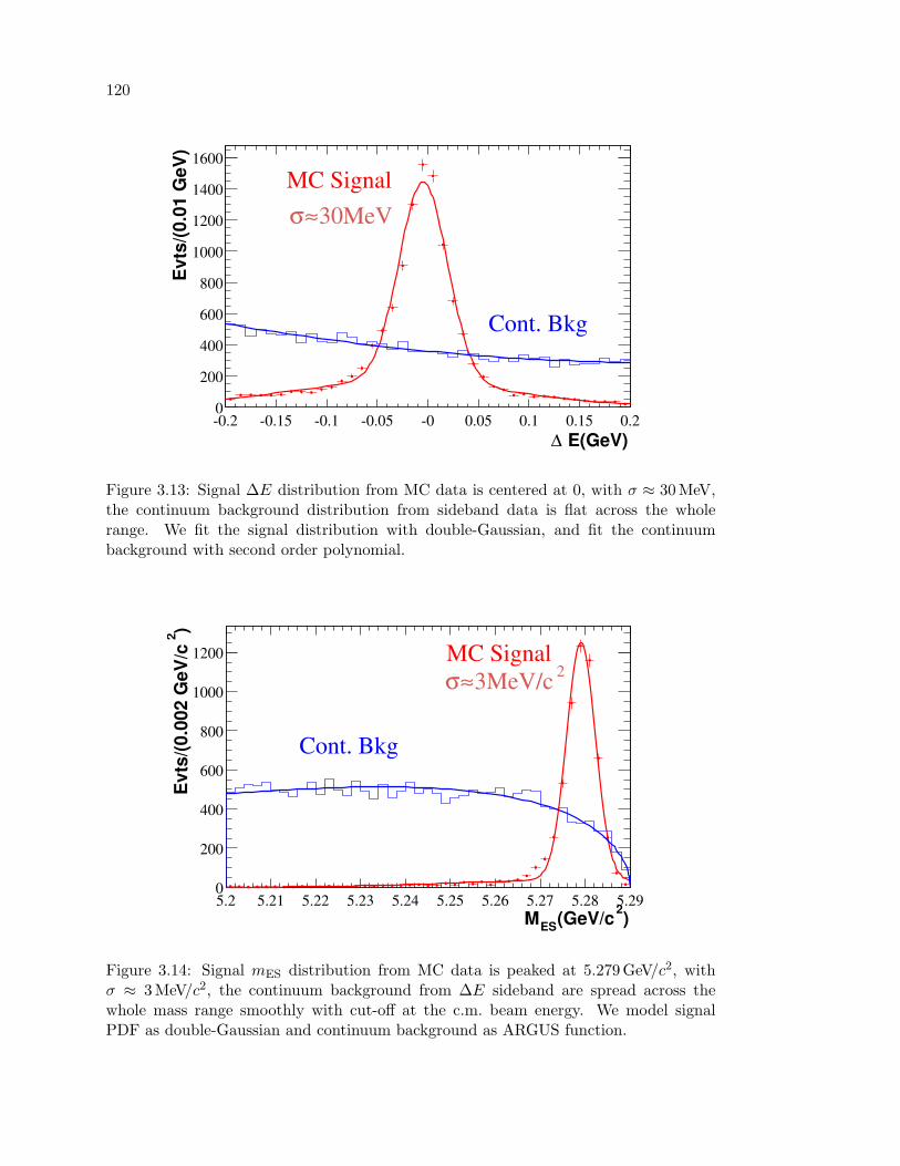
120

E(GeV)∆-0.2 -0.15 -0.1 -0.05 -0 0.05 0.1 0.15 0.2

Evt

s/(0

.01

GeV

)

0

200

400

600

800

1000

1200

1400

1600

30MeV≈σMC Signal

Cont. Bkg

Figure 3.13: Signal ∆E distribution from MC data is centered at 0, with σ ≈ 30 MeV,the continuum background distribution from sideband data is flat across the wholerange. We fit the signal distribution with double-Gaussian, and fit the continuumbackground with second order polynomial.

)2(GeV/cESM5.2 5.21 5.22 5.23 5.24 5.25 5.26 5.27 5.28 5.29

)2E

vts/

(0.0

02 G

eV/c

0

200

400

600

800

1000

1200 MC Signal23MeV/c≈σ

Cont. Bkg

Figure 3.14: Signal mES distribution from MC data is peaked at 5.279 GeV/c2, withσ ≈ 3 MeV/c2, the continuum background from ∆E sideband are spread across thewhole mass range smoothly with cut-off at the c.m. beam energy. We model signalPDF as double-Gaussian and continuum background as ARGUS function.

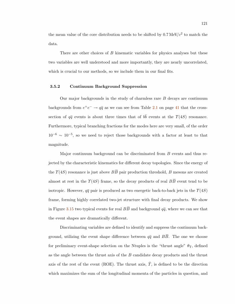
121

the mean value of the core distribution needs to be shifted by 0.7 MeV/c2 to match the

data.

There are other choices of B kinematic variables for physics analyses but these

two variables are well understood and more importantly, they are nearly uncorrelated,

which is crucial to our methods, so we include them in our final fits.

3.5.2 Continuum Background Suppression

Our major backgrounds in the study of charmless rare B decays are continuum

backgrounds from e+e− → qq as we can see from Table 2.1 on page 41 that the cross-

section of qq events is about three times that of bb events at the Υ (4S) resonance.

Furthermore, typical branching fractions for the modes here are very small, of the order

10−6 ∼ 10−5, so we need to reject those backgrounds with a factor at least to that

magnitude.

Major continuum background can be discriminated from B events and thus re-

jected by the characteristic kinematics for different decay topologies. Since the energy of

the Υ (4S) resonance is just above BB pair production threshold, B mesons are created

almost at rest in the Υ (4S) frame, so the decay products of real BB event tend to be

isotropic. However, qq pair is produced as two energetic back-to-back jets in the Υ (4S)

frame, forming highly correlated two-jet structure with final decay products. We show

in Figure 3.15 two typical events for real BB and background qq, where we can see that

the event shapes are dramatically different.

Discriminating variables are defined to identify and suppress the continuum back-

ground, utilizing the event shape difference between qq and BB. The one we choose

for preliminary event-shape selection on the Ntuples is the “thrust angle” θT, defined

as the angle between the thrust axis of the B candidate decay products and the thrust

axis of the rest of the event (ROE). The thrust axis, T , is defined to be the direction

which maximizes the sum of the longitudinal momenta of the particles in question, and

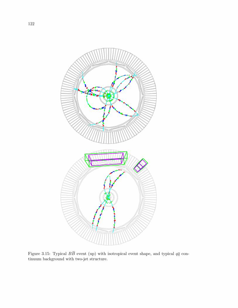
122

Figure 3.15: Typical BB event (up) with isotropical event shape, and typical qq con-tinuum background with two-jet structure.

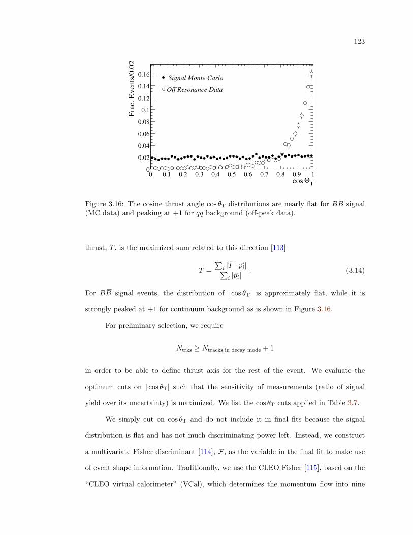
123

TΘcos 0 0.1 0.2 0.3 0.4 0.5 0.6 0.7 0.8 0.9 1

Frac

. Eve

nts/

0.02

0

0.02

0.04

0.06

0.08

0.1

0.12

0.14

0.16 Signal Monte Carlo

Off Resonance Data

Figure 3.16: The cosine thrust angle cos θT distributions are nearly flat for BB signal(MC data) and peaking at +1 for qq background (off-peak data).

thrust, T , is the maximized sum related to this direction [113]

T =∑

i |T · ~pi|∑i |~pi|

. (3.14)

For BB signal events, the distribution of | cos θT| is approximately flat, while it is

strongly peaked at +1 for continuum background as is shown in Figure 3.16.

For preliminary selection, we require

Ntrks ≥ Ntracks in decay mode + 1

in order to be able to define thrust axis for the rest of the event. We evaluate the

optimum cuts on | cos θT| such that the sensitivity of measurements (ratio of signal

yield over its uncertainty) is maximized. We list the cos θT cuts applied in Table 3.7.

We simply cut on cos θT and do not include it in final fits because the signal

distribution is flat and has not much discriminating power left. Instead, we construct

a multivariate Fisher discriminant [114], F , as the variable in the final fit to make use

of event shape information. Traditionally, we use the CLEO Fisher [115], based on the

“CLEO virtual calorimeter” (VCal), which determines the momentum flow into nine

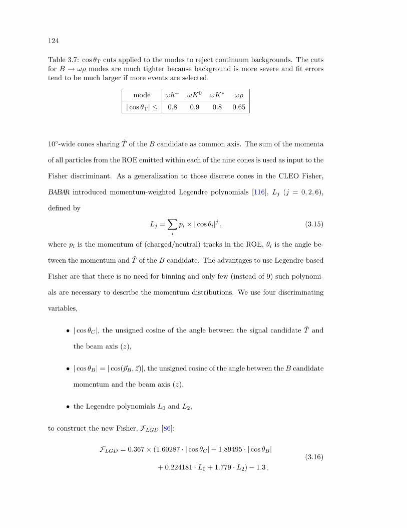
124

Table 3.7: cos θT cuts applied to the modes to reject continuum backgrounds. The cutsfor B → ωρ modes are much tighter because background is more severe and fit errorstend to be much larger if more events are selected.

mode ωh+ ωK0 ωK∗ ωρ

| cos θT| ≤ 0.8 0.9 0.8 0.65

10-wide cones sharing T of the B candidate as common axis. The sum of the momenta

of all particles from the ROE emitted within each of the nine cones is used as input to the

Fisher discriminant. As a generalization to those discrete cones in the CLEO Fisher,

BABAR introduced momentum-weighted Legendre polynomials [116], Lj (j = 0, 2, 6),

defined by

Lj =∑

i

pi × | cos θi|j , (3.15)

where pi is the momentum of (charged/neutral) tracks in the ROE, θi is the angle be-

tween the momentum and T of the B candidate. The advantages to use Legendre-based

Fisher are that there is no need for binning and only few (instead of 9) such polynomi-

als are necessary to describe the momentum distributions. We use four discriminating

variables,

• | cos θC |, the unsigned cosine of the angle between the signal candidate T and

the beam axis (z),

• | cos θB| = | cos(~pB, ~z)|, the unsigned cosine of the angle between theB candidate

momentum and the beam axis (z),

• the Legendre polynomials L0 and L2,

to construct the new Fisher, FLGD [86]:

FLGD = 0.367× (1.60287 · | cos θC |+ 1.89495 · | cos θB|

+ 0.224181 · L0 + 1.779 · L2)− 1.3 ,(3.16)

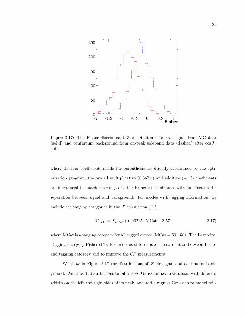
125

Fisher-2 -1.5 -1 -0.5 0 0.5 10

50

100

150

200

250

Figure 3.17: The Fisher discriminant F distributions for real signal from MC data(solid) and continuum background from on-peak sideband data (dashed) after cos θTcuts.

where the four coefficients inside the parenthesis are directly determined by the opti-

mization program, the overall multiplicative (0.367×) and additive (−1.3) coefficients

are introduced to match the range of other Fisher discriminants, with no effect on the

separation between signal and background. For modes with tagging information, we

include the tagging categories in the F calculation [117]

FLTC = FLGD + 0.06225 ·MCat− 3.57 , (3.17)

where MCat is a tagging category for all tagged events (MCat = 50−58). The Legendre-

Tagging-Category Fisher (LTCFisher) is used to remove the correlation between Fisher

and tagging category and to improve the CP measurements.

We show in Figure 3.17 the distributions of F for signal and continuum back-

ground. We fit both distributions to bifurcated Gaussian, i.e., a Gaussian with different

widths on the left and right sides of its peak, and add a regular Gaussian to model tails

126

for backgrounds. The shape of Fisher is correlated with cos θT cut because they both

use the same kind of information, and tighter cos θT cut means less discriminating power

for F . Every time cos θT cut changes, the F PDF parameters need to be adjusted.

For preliminary selection on Ntuples, we require wide range of −3 < F < 4 (the

scale of Figure 3.17 is enlarged to see the detail of the distributions).

3.5.3 BB Background

Other major backgrounds for our analyses are from real B events, including the

dominant b→ c decays of B and other rare B decays with similar decay topologies.

Usually b → c decays have negligible effects on charmless B decays, because the

products of charmless (quasi-)two-body decays have very high momenta compared with

those from charmed decays. But the charmed backgrounds could be a problem if the

two charmless mesons from B are not very light, which is the case for B → ωK∗ and

B → ωρ decays. We use generic BB MC samples to study the charmed backgrounds

for our modes, and find that peaking charmed backgrounds are really negligible to all

of our modes studied here. We just need to include systematic errors for this type of

backgrounds.

Studies using charmless BB MC data indicate that cross-feeds from other rare B

decays to the PV modes are also negligible, however, these BB backgrounds can not

be neglected in our V V modes because of heavier masses and broader mass widths of

K∗ and ρ. For the V V modes, we need to model the BB background distributions and

include them in our final fits.

First, we run Q2BApp jobs using the charmless BB MC sample with the same

settings as to our signal MC samples, then we apply the same preliminary cuts as

on real data or signal MC on the Ntuples from charmless BB MC, and we also veto

signal events or overestimated JETSET events by scanning the MC truth trees. Only

a few events (several hundred – ∼2K) in the charmless BB Ntuples pass those cuts

127

for each mode, and we go through the decay trees of those charmless events to identify

the dominant charmless backgrounds. Finally, we use exclusive SP4 MC (typical size

of 40k–80K events) of these dominant background modes and apply the preliminary

selection requirements. Those exclusive MC data provide higher statistics samples to

search for backgrounds at a level below 1%, and allow determination of their selection

efficiency with greater accuracy than provided by the charmless MC sample. Table 3.8

and 3.9 show the dominant backgrounds for each of the five V V (sub-)modes. The

estimated branching ratios are from other measurements or a guess guided by theory

when there are no measurements, and we also re-estimate the cross-feeds from modes

we are measuring after we unblind.

For each V V mode, we combine all its major BB background decays to make a

cocktail sample with appropriate proportion of number of events for each of them. The

cocktail data are then used to get BB background PDFs. Those BB background PDFs

usually do not have typical shapes common to all the five modes. Unlike continuum

backgrounds, distributions of ∆E and mES do have peaking structures, with shifted

∆E central value and broader widths for ∆E and mES. The reason for this is mainly

due to mis-reconstructed real B’s. BB background can also have the real B daughter

resonances in question, especially for ω, because of its narrow width and decay topol-

ogy. K∗/ρ have much larger widths, so the distributions are much wider and flatter,

mostly due to combinatorial and mis-reconstructed contributions. The Fisher for BB

backgrounds is also fitted with bifurcated Gaussian with the mean of the distribution in

between those of signals and continuum backgrounds. Helicity distributions are pretty

flat, and we do not expect much difference between real and combinatorial resonance, so

we just fit them with one high order polynomial component. We show in Figure 3.18 ex-

ample distributions of ∆E, mES, two resonance masses, H, and F for BB backgrounds.

Due to limited statistics, parameters of BB background PDFs have large errors. We

include this effect in our systematic studies.

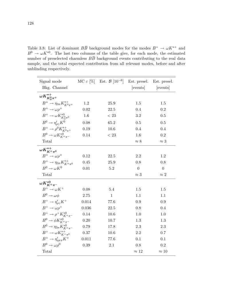
128

Table 3.8: List of dominant BB background modes for the modes B+ → ωK∗+ andB0 → ωK∗0. The last two columns of the table give, for each mode, the estimatednumber of preselected charmless BB background events contributing to the real datasample, and the total expected contribution from all relevant modes, before and afterunblinding respectively.

Signal mode MC ε [%] Est. B [10−6] Est. presel. Est. presel.Bkg. Channel [events] [events]

ωK∗+K0

Sπ+

B+ → η3πK∗+K0π+ 1.2 25.9 1.5 1.5

B+ → ωρ+ 0.02 22.5 0.4 0.2B+ → ωK∗0

K0Sπ0 1.6 < 23 3.2 0.5

B0 → η′ργK0 0.08 65.2 0.5 0.5

B+ → ρ0K∗+K0π+ 0.19 10.6 0.4 0.4

B0 → ωK∗0K+π− 0.14 < 23 1.6 0.2

Total ≈ 8 ≈ 3

ωK∗+K+π0

B+ → ωρ+ 0.12 22.5 2.2 1.2B+ → η3πK

∗+K+π0 0.45 25.9 0.8 0.8

B0 → ωK0 0.01 5.2 0 0Total ≈ 3 ≈ 2

ωK∗0K+π−

B+ → ωK+ 0.08 5.4 1.5 1.5B0 → ωφ 2.75 1 1.1 1.1B+ → η′ργK

+ 0.014 77.6 0.9 0.9B+ → ωρ+ 0.036 22.5 0.8 0.4B+ → ρ+K∗0

K+π− 0.14 10.6 1.0 1.0B0 → φK∗0

K+π− 0.20 10.7 1.3 1.3B0 → η3πK

∗0K+π− 0.79 17.8 2.3 2.3

B+ → ωK∗+K+π0 0.37 10.6 2.2 0.7

B+ → η′ηππK+ 0.011 77.6 0.1 0.1

B0 → ωρ0 0.39 2.1 0.8 0.2Total ≈ 12 ≈ 10

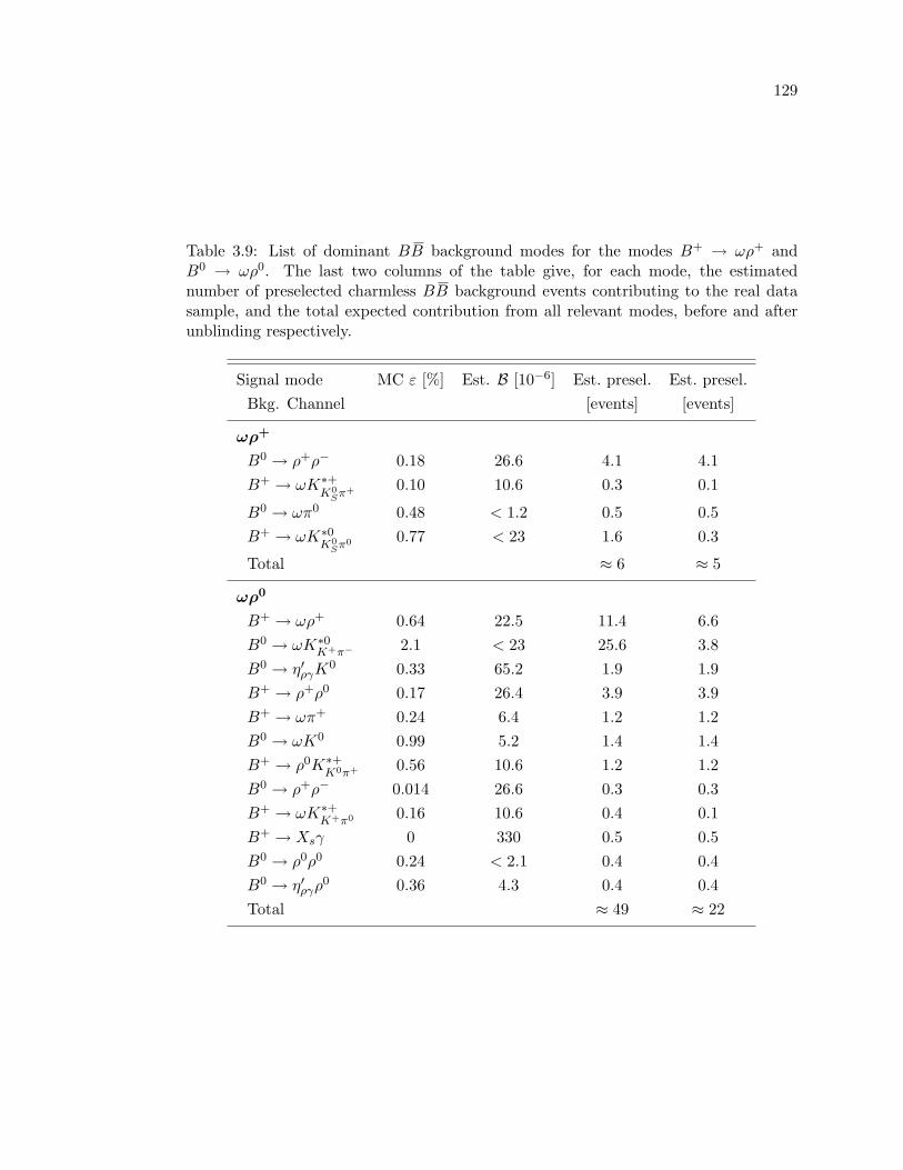
129

Table 3.9: List of dominant BB background modes for the modes B+ → ωρ+ andB0 → ωρ0. The last two columns of the table give, for each mode, the estimatednumber of preselected charmless BB background events contributing to the real datasample, and the total expected contribution from all relevant modes, before and afterunblinding respectively.

Signal mode MC ε [%] Est. B [10−6] Est. presel. Est. presel.Bkg. Channel [events] [events]

ωρ+

B0 → ρ+ρ− 0.18 26.6 4.1 4.1B+ → ωK∗+

K0Sπ+ 0.10 10.6 0.3 0.1

B0 → ωπ0 0.48 < 1.2 0.5 0.5B+ → ωK∗0

K0Sπ0 0.77 < 23 1.6 0.3

Total ≈ 6 ≈ 5

ωρ0

B+ → ωρ+ 0.64 22.5 11.4 6.6B0 → ωK∗0

K+π− 2.1 < 23 25.6 3.8B0 → η′ργK

0 0.33 65.2 1.9 1.9B+ → ρ+ρ0 0.17 26.4 3.9 3.9B+ → ωπ+ 0.24 6.4 1.2 1.2B0 → ωK0 0.99 5.2 1.4 1.4B+ → ρ0K∗+

K0π+ 0.56 10.6 1.2 1.2B0 → ρ+ρ− 0.014 26.6 0.3 0.3B+ → ωK∗+

K+π0 0.16 10.6 0.4 0.1B+ → Xsγ 0 330 0.5 0.5B0 → ρ0ρ0 0.24 < 2.1 0.4 0.4B0 → η′ργρ

0 0.36 4.3 0.4 0.4Total ≈ 49 ≈ 22

130

)2(E) (GeV/c∆-0.2 -0.15 -0.1 -0.05 -0 0.05 0.1 0.15 0.2

Eve

nts

/ ( 0

.01

GeV

)

0

2

4

6

8

10

12

14

16

18

0.092± = 0.278 coref 0.0086± = -0.07135 coreµ

0.36± = -0.200 tailµ 0.011± = 0.036 coreσ

0.20± = 0.44 tailσ/n = 1.1322χ

)2(E) (GeV/c∆-0.2 -0.15 -0.1 -0.05 -0 0.05 0.1 0.15 0.2

Eve

nts

/ ( 0

.01

GeV

)

0

2

4

6

8

10

12

14

16

18a)

)2 (GeV/cesm5.2 5.21 5.22 5.23 5.24 5.25 5.26 5.27 5.28 5.29

Eve

nts

/ ( 0

.002

GeV

)

0

2

4

6

8

10

12

14

0.0019± = 5.2751 µ 0.0043± = 0.0122 σ

1.0±Tail = 1.4 /n = 0.7182χ

)2 (GeV/cesm5.2 5.21 5.22 5.23 5.24 5.25 5.26 5.27 5.28 5.29

Eve

nts

/ ( 0

.002

GeV

)

0

2

4

6

8

10

12

14b)

)2 (GeV/cωm0.74 0.75 0.76 0.77 0.78 0.79 0.8 0.81 0.82

Eve

nts

/ ( 0

.002

)

0

2

4

6

8

10

12

14

16

18

0.26±Cub = 0.35 0.096± = 0.589 sigf

0.0010± = 0.7837 coreµ 0.38±Quad = 0.23 0.0011± = 0.0078 coreσ 0.23±Slope = 0.05

/n = 0.6212χ

)2 (GeV/cωm0.74 0.75 0.76 0.77 0.78 0.79 0.8 0.81 0.82

Eve

nts

/ ( 0

.002

)

0

2

4

6

8

10

12

14

16

18

c)

)2 (GeV/cρm0.6 0.7 0.8 0.9 1

Eve

nts

/ ( 0

.028

9474

)

0

5

10

15

20

25

0.35±Cub = 0.22 0.39± = 0.37 sigf

0.060± = 0.636 coreµ 0.76±Quad = -0.561

0.046± = 0.088 coreσ 1.1±Slope = -0.06

/n = 0.4562χ

)2 (GeV/cρm0.6 0.7 0.8 0.9 1

Eve

nts

/ ( 0

.028

9474

)

0

5

10

15

20

25 d)

Hel)ωcos(0 0.1 0.2 0.3 0.4 0.5 0.6 0.7 0.8 0.9 1

Eve

nts

/ ( 0

.02

)

0

2

4

6

8

10

12

0.048± = -0.7151 Cp1 0.051± = -0.0404 Cp2 0.055± = -0.3032 Cp3

/n = 0.9312χ

Hel)ωcos(0 0.1 0.2 0.3 0.4 0.5 0.6 0.7 0.8 0.9 1

Eve

nts

/ ( 0

.02

)

0

2

4

6

8

10

12

e)

Hel)ρcos(-0.6 -0.4 -0.2 -0 0.2 0.4 0.6 0.8

Eve

nts

/ ( 0

.036

25 )

0

2

4

6

8

10 0.73± = 0.97 Cp1

1.5± = 2.2 Cp2 2.4± = -1.27 Cp3

/n = 0.7582χ

Hel)ρcos(-0.6 -0.4 -0.2 -0 0.2 0.4 0.6 0.8

Eve

nts

/ ( 0

.036

25 )

0

2

4

6

8

10f)

Fisher-3 -2 -1 0 1 2 3 4

Eve

nts

/ ( 0

.2 )

0

5

10

15

20

25

30 0.087± = -0.4879 coreµ

0.057± = 0.452 lCoreσ 0.055± = 0.355 rCoreσ

/n = 0.1152χ

Fisher-3 -2 -1 0 1 2 3 4

Eve

nts

/ ( 0

.2 )

0

5

10

15

20

25

30g)

Figure 3.18: BB background distributions of a) ∆E, b) mES, c) ω mass, d) ρ mass, e)ω H, f) ρ H, and g) F , for B → ωρ modes using cocktails of exclusive charmless signalMC data.

131

3.6 Maximum Likelihood Fit

In this section, we will discuss the main method, maximum likelihood [118] (ML)

fit, that we use to extract final results. We will also describe several details with respect

to the fit not explained in previous sections, and finally we discuss the validation of these

methods. For general information on the statistic tools, methods, or terminologies, see

for example, Ref. 119, and the Statistics Review of Ref. 12.

From an experimental point of view, the branching fraction of a B decay can be

written as

B =Nobs

ε×NBB

, (3.18)

where Nobs is the ML fit bias corrected (see Sec. 3.6.4.1) number of observed signal

events, NBB is the total number of BB pairs in the sample, and ε is the total efficiency

of the analysis, i.e., the ratio of Nobs to the number of signal events in the sample. For

a given sample, we may have already known NBB, and we can use MC simulation to

study the efficiencies of our analyses, which is not too difficult. Our main task is to

extract the signal yields, Nobs.

Two methods are mainly used to get the signal yields: “Cut & Count” method and

parameter estimation method based on likelihood function. In “Cut & Count” method,

one needs to make much tighter cuts then we have applied in previous sections, and

those cuts can be optimized, for example, to maximize the signal-to-background ratioN2

S

NS +NB, where NS and NB are the numbers of (expected) signal and background

events. The signal region for this method is usually much smaller (typical within ∼ 2σ

of the mean values) than we defined (see Sec. 3.5.1) in order to have clean signals. So

the efficiency for this method is very low which is not suitable for rare decay studies

performed here, and we mainly, if any, use this method as cross check.

To extract signal yields for charmless rare B decays, we primarily use an unbinned,

extended multivariate ML fit [120] based on the maximum likelihood method. A number

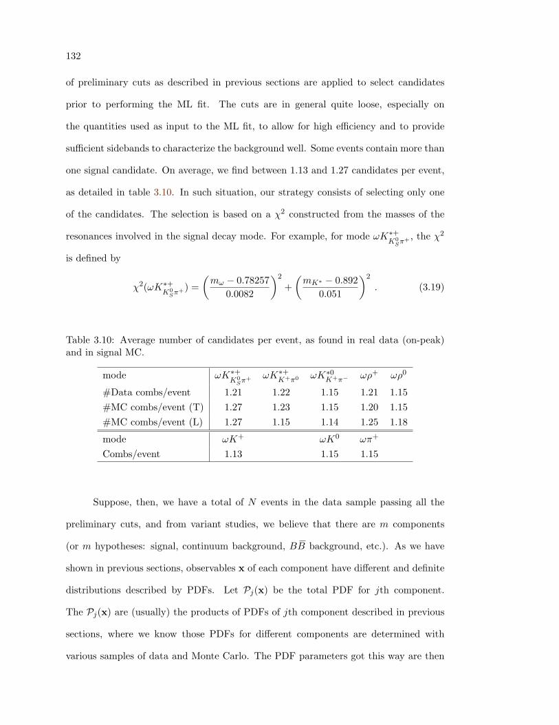
132

of preliminary cuts as described in previous sections are applied to select candidates

prior to performing the ML fit. The cuts are in general quite loose, especially on

the quantities used as input to the ML fit, to allow for high efficiency and to provide

sufficient sidebands to characterize the background well. Some events contain more than

one signal candidate. On average, we find between 1.13 and 1.27 candidates per event,

as detailed in table 3.10. In such situation, our strategy consists of selecting only one

of the candidates. The selection is based on a χ2 constructed from the masses of the

resonances involved in the signal decay mode. For example, for mode ωK∗+K0

Sπ+ , the χ2

is defined by

χ2(ωK∗+K0

Sπ+) =(mω − 0.78257

0.0082

)2

+(mK∗ − 0.892

0.051

)2

. (3.19)

Table 3.10: Average number of candidates per event, as found in real data (on-peak)and in signal MC.

mode ωK∗+K0


K+π− ωρ+ ωρ0

#Data combs/event 1.21 1.22 1.15 1.21 1.15#MC combs/event (T) 1.27 1.23 1.15 1.20 1.15#MC combs/event (L) 1.27 1.15 1.14 1.25 1.18

mode ωK+ ωK0 ωπ+

Combs/event 1.13 1.15 1.15

Suppose, then, we have a total of N events in the data sample passing all the

preliminary cuts, and from variant studies, we believe that there are m components

(or m hypotheses: signal, continuum background, BB background, etc.). As we have

shown in previous sections, observables x of each component have different and definite

distributions described by PDFs. Let Pj(x) be the total PDF for jth component.

The Pj(x) are (usually) the products of PDFs of jth component described in previous

sections, where we know those PDFs for different components are determined with

various samples of data and Monte Carlo. The PDF parameters got this way are then

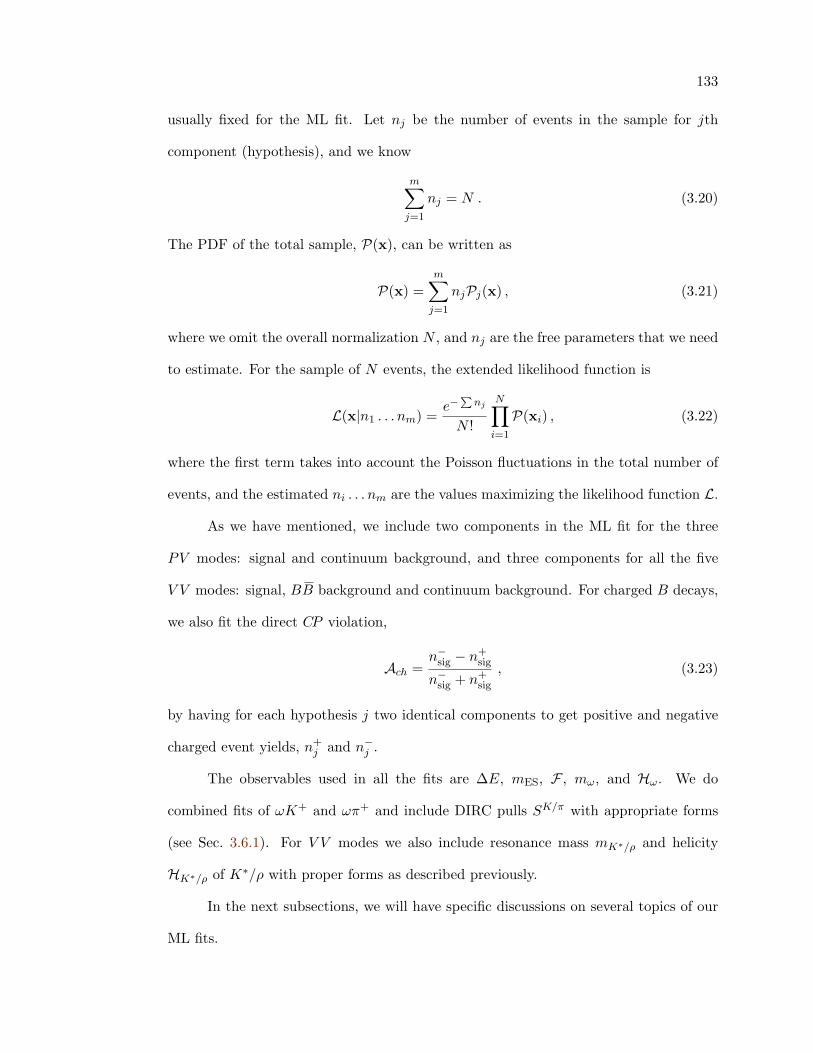
133

usually fixed for the ML fit. Let nj be the number of events in the sample for jth

component (hypothesis), and we know

m∑j=1

nj = N . (3.20)

The PDF of the total sample, P(x), can be written as

P(x) =m∑

j=1

njPj(x) , (3.21)

where we omit the overall normalization N , and nj are the free parameters that we need

to estimate. For the sample of N events, the extended likelihood function is

L(x|n1 . . . nm) =e−

Pnj

N !

N∏i=1

P(xi) , (3.22)

where the first term takes into account the Poisson fluctuations in the total number of

events, and the estimated ni . . . nm are the values maximizing the likelihood function L.

As we have mentioned, we include two components in the ML fit for the three

PV modes: signal and continuum background, and three components for all the five

V V modes: signal, BB background and continuum background. For charged B decays,

we also fit the direct CP violation,

Ach =n−sig − n+

sig

n−sig + n+sig

, (3.23)

by having for each hypothesis j two identical components to get positive and negative

charged event yields, n+j and n−j .

The observables used in all the fits are ∆E, mES, F , mω, and Hω. We do

combined fits of ωK+ and ωπ+ and include DIRC pulls SK/π with appropriate forms

(see Sec. 3.6.1). For V V modes we also include resonance mass mK∗/ρ and helicity

HK∗/ρ of K∗/ρ with proper forms as described previously.

In the next subsections, we will have specific discussions on several topics of our

ML fits.

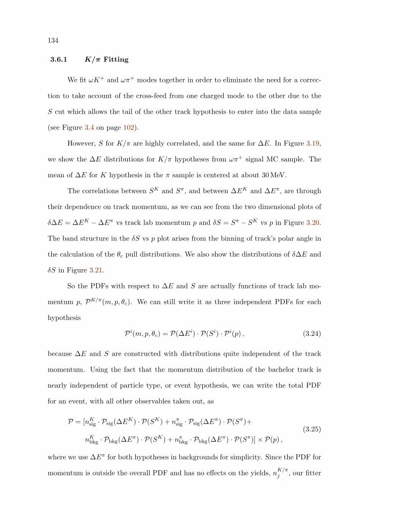
134

3.6.1 K/π Fitting

We fit ωK+ and ωπ+ modes together in order to eliminate the need for a correc-

tion to take account of the cross-feed from one charged mode to the other due to the

S cut which allows the tail of the other track hypothesis to enter into the data sample

(see Figure 3.4 on page 102).

However, S for K/π are highly correlated, and the same for ∆E. In Figure 3.19,

we show the ∆E distributions for K/π hypotheses from ωπ+ signal MC sample. The

mean of ∆E for K hypothesis in the π sample is centered at about 30 MeV.

The correlations between SK and Sπ, and between ∆EK and ∆Eπ, are through

their dependence on track momentum, as we can see from the two dimensional plots of

δ∆E = ∆EK −∆Eπ vs track lab momentum p and δS = Sπ − SK vs p in Figure 3.20.

The band structure in the δS vs p plot arises from the binning of track’s polar angle in

the calculation of the θc pull distributions. We also show the distributions of δ∆E and

δS in Figure 3.21.

So the PDFs with respect to ∆E and S are actually functions of track lab mo-

mentum p, PK/π(m, p, θc). We can still write it as three independent PDFs for each

hypothesis

P i(m, p, θc) = P(∆Ei) · P(Si) · P i(p) , (3.24)

because ∆E and S are constructed with distributions quite independent of the track

momentum. Using the fact that the momentum distribution of the bachelor track is

nearly independent of particle type, or event hypothesis, we can write the total PDF

for an event, with all other observables taken out, as

P = [nKsig · Psig(∆EK) · P(SK) + nπ

sig · Psig(∆Eπ) · P(Sπ)+

nKbkg · Pbkg(∆Eπ) · P(SK) + nπ

bkg · Pbkg(∆Eπ) · P(Sπ)]× P(p) ,(3.25)

where we use ∆Eπ for both hypotheses in backgrounds for simplicity. Since the PDF for

momentum is outside the overall PDF and has no effects on the yields, nK/πj , our fitter

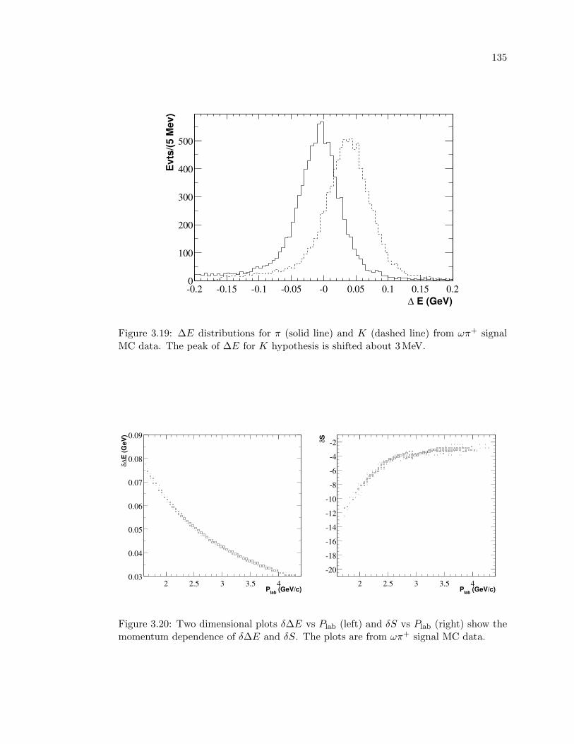
135

E (GeV)∆-0.2 -0.15 -0.1 -0.05 -0 0.05 0.1 0.15 0.2

Evt

s/(5

Mev

)

0

100

200

300

400

500

Figure 3.19: ∆E distributions for π (solid line) and K (dashed line) from ωπ+ signalMC data. The peak of ∆E for K hypothesis is shifted about 3 MeV.

(GeV/c)labP2 2.5 3 3.5 4

E (G

eV)

∆δ

0.03

0.04

0.05

0.06

0.07

0.08

0.09

(GeV/c)labP2 2.5 3 3.5 4

Sδ

-20

-18

-16

-14

-12

-10

-8

-6

-4

-2

Figure 3.20: Two dimensional plots δ∆E vs Plab (left) and δS vs Plab (right) show themomentum dependence of δ∆E and δS. The plots are from ωπ+ signal MC data.

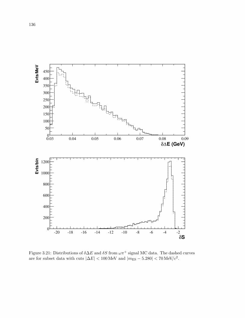
136

E (GeV)∆δ0.03 0.04 0.05 0.06 0.07 0.08 0.09

Evt

s/M

eV

0

50

100

150

200

250

300

350

400

450

Sδ-20 -18 -16 -14 -12 -10 -8 -6 -4 -2

Evt

s/bi

n

0

200

400

600

800

1000

1200

Figure 3.21: Distributions of δ∆E and δS from ωπ+ signal MC data. The dashed curvesare for subset data with cuts |∆E| < 100 MeV and |mES − 5.280| < 70 MeV/c2.

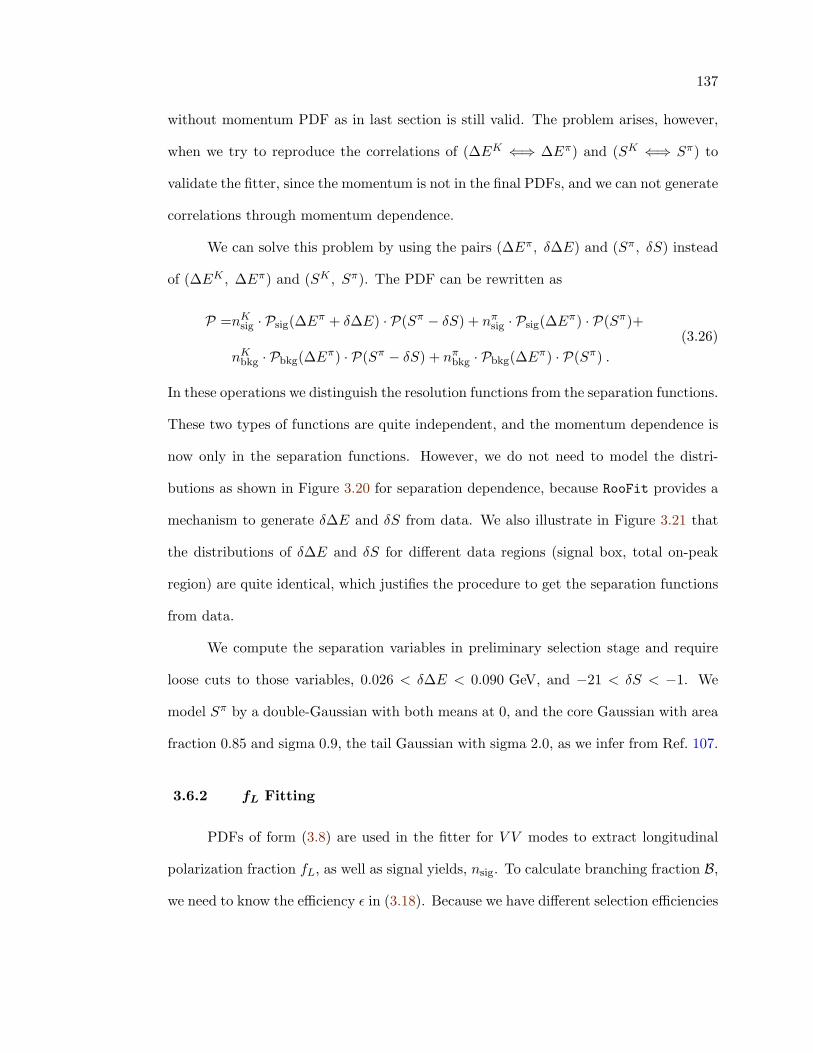
137

without momentum PDF as in last section is still valid. The problem arises, however,

when we try to reproduce the correlations of (∆EK ⇐⇒ ∆Eπ) and (SK ⇐⇒ Sπ) to

validate the fitter, since the momentum is not in the final PDFs, and we can not generate

correlations through momentum dependence.

We can solve this problem by using the pairs (∆Eπ, δ∆E) and (Sπ, δS) instead

of (∆EK , ∆Eπ) and (SK , Sπ). The PDF can be rewritten as

P =nKsig · Psig(∆Eπ + δ∆E) · P(Sπ − δS) + nπ

sig · Psig(∆Eπ) · P(Sπ)+

nKbkg · Pbkg(∆Eπ) · P(Sπ − δS) + nπ

bkg · Pbkg(∆Eπ) · P(Sπ) .(3.26)

In these operations we distinguish the resolution functions from the separation functions.

These two types of functions are quite independent, and the momentum dependence is

now only in the separation functions. However, we do not need to model the distri-

butions as shown in Figure 3.20 for separation dependence, because RooFit provides a

mechanism to generate δ∆E and δS from data. We also illustrate in Figure 3.21 that

the distributions of δ∆E and δS for different data regions (signal box, total on-peak

region) are quite identical, which justifies the procedure to get the separation functions

from data.

We compute the separation variables in preliminary selection stage and require

loose cuts to those variables, 0.026 < δ∆E < 0.090 GeV, and −21 < δS < −1. We

model Sπ by a double-Gaussian with both means at 0, and the core Gaussian with area

fraction 0.85 and sigma 0.9, the tail Gaussian with sigma 2.0, as we infer from Ref. 107.

3.6.2 fL Fitting

PDFs of form (3.8) are used in the fitter for V V modes to extract longitudinal

polarization fraction fL, as well as signal yields, nsig. To calculate branching fraction B,

we need to know the efficiency ε in (3.18). Because we have different selection efficiencies

138

for longitudinal and transverse components, the total efficiency ε is a function of fL:

ε = fL · εL + (1− fL) · εT , (3.27)

where εL and εT are MC efficiencies for longitudinal and transverse components, respec-

tively. So the uncertainty of fL can transfer to ε, and to the branching fraction B, as

well as from nsig to B. It is then convenient to fit branching fraction instead of signal

yields in the ML fit. For this purpose, we write nsig as a function of εL, εT , fL, B, and

NBB, where fL and B are free parameters to fit. We actually have two fit options for

V V modes, one is the regular fitter to get signal yields and significance, another one

fits directly to get branching fractions.

3.6.3 Floating Continuum Background Parameters

Within the framework of RooFit we have the ability to float some of the PDF

parameters in the final ML fit. By doing this, continuum background parameters can

be determined by making use of the larger statistics available in the full on-peak sample

rather than restricting the data to on-peak sidebands. When we initially determine

PDFs for our variables, we project onto a specific variable. As a result, the fitter must

minimize only a handful of parameters. When we choose to float background parameters

in the final ML fit, our fitter must be able to find a minimum in a larger-parameter

space. We have tested that our fitter can handle the number of degrees of freedom we

use in our final fits (typically 12 ∼ 16).

For the analyses described here, we choose to float the most important parameters

in the continuum background, including ARGUS exponent ξ, ∆E coefficients, core

parameters of Fisher, combinatorial background fractions and slopes for resonances. We

do not, however, float parameters for signal components, but determine them from the

signal Monte Carlo (including appropriate corrections as described in previous sections.

Additionally, we do not float parameters to which our signal yields are insensitive (such

139

as tail components of peaking backgrounds). For all parameters floated in our analyses,

we initialize their values to those determined from sideband data.

3.6.4 Fit Validation

We build our ML fitter based on several assumptions, and we use this fitter to

get our final results. The correctness of our results relies on the correctness of those

assumptions and the fitter itself. We must make sure that the analysis is fully validated

before we fit to get the results.

We include one or two background components in the fitter and assume others

are negligible, which we have to test carefully. We use various data and Monte Carlo

samples to check for possible backgrounds. Usually we run our physics analysis job

Q2BApp on those samples with the same setting as on real or signal MC data and apply

the same preliminary selection cuts to the Ntuples of those samples. If the number of

events passing the cuts is really small, the background from that particular sample can

be neglected safely. Otherwise, we have to include a component in the ML fit for that

background, or find a method to suppress it.

The PDF for each component included in the ML fit is usually the product of

several PDFs of individual observables. By doing this, we assume that the observables

are independent to each other. We choose observables so as to minimize the correla-

tion between them, but these observables are not totally independent. We check the

correlation between observables by measuring the correlation coefficients, r(x, y),

r(x, y) =

∑i

(xi − x)(yi − y)√∑i

(xi − x)2∑

i

(yi − y)2. (3.28)

We find that for all the modes studied here, none of the coefficients is larger than 6%,

and by far most are below 1%, justifying our procedure. (Detailed studies on observable

correlations are performed for individual modes if particular correlations are expected

140

for those modes. See Chapter 4 for detailed discussions.) Correlation between ARGUS

exponent and Fisher [121] is found common to most of our analyses and Q2BFit has

been modified to allow fitting for such a correlation [112]. The effects on the final results

are found negligible for modes in this work.

We model our signal PDFs mainly from signal MC samples, which could give us

parameters slightly different from what they should be in the real data. We use control

samples, or if the statistics allow, use our data sample directly to correct any differences.

As we have discussed, we have applied ω mass scale and shift corrections, ∆E width

scale, mES mean shift, S shape corrections, etc., to our PDF parameters.

3.6.4.1 Fit Bias

The residual effects due to the correlations in the signal and other imperfection in

modeling the PDFs are taken into account in the “ML-fit bias”, or the ML fit efficiency,

correction.

One of our tests for bias in the fit method is to generate samples of events drawn

from the background PDFs into which we embed a known number of events selected

randomly from the signal MC sample. We express the fit bias factor as the ratio of

(and/or the difference between) the mean yield from the fit to the number of embedded

signal events.

3.6.4.2 Goodness-of-Fit Test

One test of the overall fitting procedure is to check the goodness-of-fit [122].

This is defined as how well the χ2 of the fit to the on-peak data compares with the

distribution of fit χ2 obtained from fit to the data samples generated from the fitter

itself. One should expect the measured value to lie with a few sigma of the mean of the

generated distributions. The goodness-of-fit test is performed after unblinding.

141

3.6.5 Signal Significance and Upper Limit

Once we fit the final results, we make the test of signal significance [123], which is

the maximum likelihood ratio of the central yield value against the null hypothesis. The

ratio is the number of standard deviations of a Gaussian distribution at which point the

probability corresponds to that for a null hypothesis to fluctuate to the observed yield.

We may claim an observation if the signal significance is greater than 4σ. Otherwise,

we calculate the 90% confidence level (CL) upper limit (UL) for the branching fraction,

which means a probability of 90% that the real branching fraction is below that limit.

We use a procedure described in Sec. 3.7.1 to calculate the ULs with systematics included

in the calculation.

3.7 Systematic Errors

The branching fractions measured have systematic as well as statistical uncertain-

ties, including those from the number of NBB (Eq. 3.18), ML fits, various efficiencies

and production rates.

B Counting Errors

We take the number of produced BB pairs in the sample from the luminosity

and B counting script [124], which selects inclusive hadronic events in both on- and

off-peak data sets and measures the number of BB pairs through the increase in the

ratio of hadronic events to muon pairs between on- and off-peak data sets due to Υ (4S)

production. We assume equal numbers of charged and neutral B’s, and determine the

error on the number of BB events from the script to be 1.1%, which is mainly due to

the uncertainty of the MC simulation for the GoodTracksLoose candidate list.

142

ML Fit Errors

We divide systematic errors from ML fit into two categories: the fit bias (or fit

efficiency), which is mainly due to observable correlations, as described in Sec. 3.6.4.1,

and yield error, which is due to the uncertainties of PDF parameters. We take one-half

of the fit bias as systematic errors from the fit bias.

In order to determine the ML fit yield systematic, we would like to float PDF

signal parameters in the fit. For modes with a small number of signal events, however,

this is not practical. As an alternative, we use control samples, or the on-peak sideband

data if statistics allowed, to study how well the MC models the data, and apply ap-

propriate corrections (see Sec. 3.6.4). From these studies, we also determine values by

which to vary our signal parameters around these nominal values. We set the variations

for signal PDF parameters which have no such studies to their errors from parameter

fitting procedures. We then apply these variations, one at a time, to our signal PDFs

and re-run the ML fit. We quote the changes in the yields as systematic errors for the

parameter uncertainties, and add all these errors quadratically to get the ML fit yield

error.

Efficiency Errors

The MC signal efficiency is determined by the ratio of the events used in the fit

and the total number of generated MC signal events. To obtain the final efficiency,

the MC efficiency has to be corrected for the overestimate of the tracking and neutral

efficiencies in the simulation. For the K0S efficiency we take the correction determined

for the selection we use from Ref. 103. We apply no correction for the K0S tracks since

the ChargedTracks list is used. Finally, the efficiency must be corrected for resonance

branching fractions since the channel of interest is forced in signal MC.

We summarize below systematic errors from efficiencies and all other sources.

143

• Trigger efficiency: The trigger efficiency for multi-hadron events is in excess of

0.9993 [124]. We neglect the systematic error on the tiny inefficiency from this

source.

• Track multiplicity: This is for the cut on the minimum number of tracks in the

event. We require the reconstruction of at least one track from the other B decay.

The signal MC inefficiency for this cut is a few percent. We assign an uncertainty

of 1%.

• Track finding/efficiency: The study of absolute tracking efficiency in Ref. 125 pro-

vides a systematic error associated with the correction tables for GoodTracksLoose

tracks of 0.8% per track.

• γ, π0 finding: The photon efficiency is overestimated in MC [94]. Following the

recommendations, we have therefore “smeared” the MC to match the data, and

calculate the systematic error per photon by adding in quadrature a fixed contri-

bution of 2.5%.

• K0S finding/efficiency: The K0

S efficiency systematic error due to displaced track

origins is conservatively estimated to be 3% [103]. The additional contribution

from different effects between GoodTracksLoose and ChargedTracks was evalu-

ated and found to be a negligible 0.25% [126]. The systematic for finding (prompt)

ChargedTracks is 1.3% per track [125]; the total K0S efficiency systematic includ-

ing this is 4%.

• Event shape cuts: There are two variables used for event shape cuts, cos θT and

F . For cos θT, the systematic uncertainty estimate is straightforward, since the

expectation is that the distribution of signal MC for this variable should be nearly

flat. We take the systematic uncertainty to be one-half of the difference between

the observed signal MC efficiency of the cos θT cut used for each analysis and the

144

expectation of a flat distribution. For F , the systematic uncertainty is included

in the ML fit yield error discussed above.

• Particle ID: The PID killing efficiency is determined from the PID tables where

data control samples determine efficiencies with an uncertainty of ∼0.1% [95] when

integrated over our samples. Thus we take the PID killing systematic error to be

negligible. For analyses with a charged kaon, we estimate that the uncertainty of

the tight kaon selector (again determined from data) to be 1%.

As we include the DIRC pull for the prompt charged track in the ML fit for ωh+,

we use the uncertainties on the PID parameterization, as determined from data

control samples [107], to vary the PDF in our fit. The resulting change in fit yield

is quoted here as the PID systematic.

• BB background: BB background is included in the fits for V V modes. In principle

this accounts for uncertainty in this yield in the statistical error. We quote the

BB background systematic to be one half the measured change in the signal yield

when the number of fit BB events is changed by one standard deviation, to allow

for uncertainties in the BB PDFs.

For PV modes in this work, we estimate the BB background is small and assign

±1 event as systematic error.

• Polarization fraction fL: Based on the BABAR measurements for ρρ and K∗ρ

modes [127], we fix the longitudinal polarization fraction fL to 0.9 for all the

V V modes at first, and if we find significant signal yield after unblinding, we will

float fL eventually.

For the results obtained from fits with fixed fL we assign the systematic on the

yield to be the measured change in branching ratio when fL is changed by 0.3

(' 1/√

12).

145

For the fit with fL free, we obtain the final branching fraction result directly from

ML fit (see Sec. 3.6.2), which gives a statistical error that fully contains the error

of branching fraction from fL.

The dominant systematic on fL itself when floated, comes from any unmodeled

correlations or other effects in the PDFs; we estimate its systematic error based on

the observed difference between the fitted means of distributions from pure PDF

generated samples and generated background with embedded signal MC samples.

• Charge Asymmetry Systematics: Systematic effects in charge asymmetry mea-

surements with similar kinematics to ωh+ decays were studied in detail in the

B+ → η′K+ analyses [86], and we assign the same systematic error of 1.1% to the

charge asymmetries.

For the analyses with a K∗ or ρ, the charged K or π used for the asymmetry has

a much wider momentum spectrum. We assign 2% systematic uncertainty for Ach

that was determined in the study of decay B → φK∗ [13].

• MC statistics: Analyses use about 40K events from the 10 series SP4 production.

With a typical efficiency of 20%, this gives a relative error of 1.0%. Actual values

are given for each mode.

• Branching fractions of daughters: This is simply taken as the uncertainty on the

branching fraction from the world averages [12].

3.7.1 Combining Results

We combine branching fractions from different decay sub-modes using their log-

likelihood curves to get one branching fraction value [112]. When combining, these

curves should be adjusted with the effects of systematic uncertainties, which can be

grouped into three types: additive systematic uncertainties, which affect the fit yield

146

and thus the statistical significance of a result, uncorrelated systematic uncertainties,

which are mode-independent, and generally are a superset of the additive systematic

uncertainties, and correlated systematic uncertainties, which affect all modes in the

same direction. Correlated errors are not applied to individual curves before combining,

because they shift all curves in the same direction due to common uncertainties on

efficiency and thus have a different effect on the combined log-likelihood curve.

Including a uncorrelated systematic uncertainty σsyst involves convoluting the

likelihood with a Gaussian of width σsyst. If the original likelihood curve is Gaussian

with width σstat, this produces a new Gaussian likelihood curve with σ2 = σ2syst + σ2

stat.

Equivalently, this adjusts the log-likelihood curve by:

χ2 =χ2

stat χ2syst

χ2stat + χ2

syst

, (3.29)

where χ2stat = (x − µ)2/σ2

stat and similarly for χ2syst. This has the effect of broadening

the log-likelihood curve to account for the systematic uncertainty. Log-likelihood curves

corrected by uncorrelated systematic errors are then added together and the new mini-

mum of the combined curve is readjusted to 0. The significance of the combined results

is

signif(σ) =√−2 ln(L/Lmax) , (3.30)

evaluated at nsig = 0. To include correlated systematic errors, the curves for individual

modes are shifted down one sigma and the mean of the combined curve is found. This

is repeated for individual curves shifting up one sigma. The average change of the

combined means is the weighted correlated systematic error. And this error is then

applied to the original combined curve with uncorrelated systematic errors included to

get the final log-likelihood curve including all systematic errors.

The combining procedure is done with a root script, combine.cc, making use of

likelihood scan curves output by Q2BFit. Detailed usage of the package can be found

in Ref. 128.

Chapter 4

Analysis Results

We present in this chapter our analyses results for charmless two-body rare B

decays with ω mesons based on BABAR Run 1 and Run 2 data with 88.9×106 BB pairs,

using analysis techniques described in the previous chapter. The results for PV modes:

B+ → ωK+, ωπ+, and B0 → ωK0, are summarized in Sec. 4.1, and V V results for

B → ωK∗ and B → ωρ are presented in Sec. 4.2. Analysis details for individual modes

are also addressed in both sections.

4.1 B+ → ωK+, ωπ+ and B0 → ωK0

The observables in the ML fit for B0 → ωK0 mode are: ∆E, mES, F , mω, and

H. We fit B+ → ωK+ and ωπ+ modes simultaneously∗ with three more observables:

δ∆E, S, and δS. A set of preliminary selection cuts appropriate for each mode are

applied to real and MC data to get final datasets. We include for each mode two

PDF components: signal and continuum background. Signal PDFs are got from signal

MC data with corrections to take account of the difference between signal and MC

data if necessary, and background PDFs are from on-peak sideband data, with major

background parameters floated to make use of larger statistics of the full on-peak data

in the final fit.

∗ For historical reason, we first implemented B+ → ωK+ and ωπ+ as separate fits [129] and laterdid K/π combined fitting.

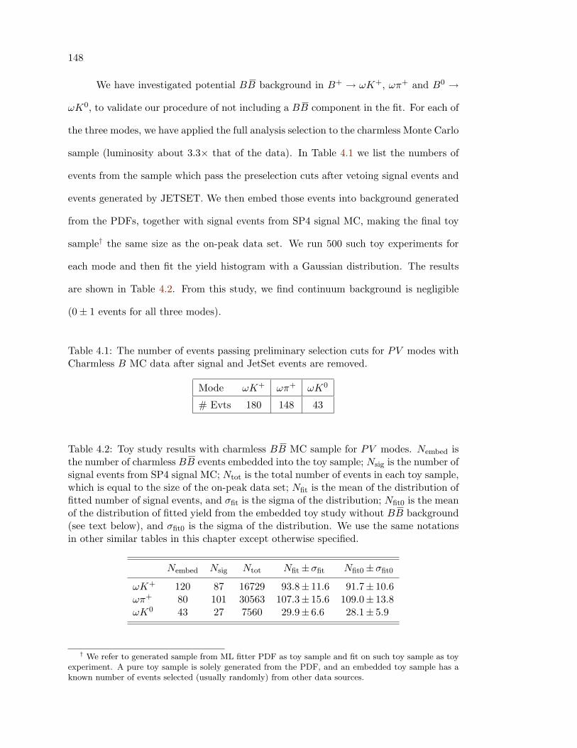
148

We have investigated potential BB background in B+ → ωK+, ωπ+ and B0 →

ωK0, to validate our procedure of not including a BB component in the fit. For each of

the three modes, we have applied the full analysis selection to the charmless Monte Carlo

sample (luminosity about 3.3× that of the data). In Table 4.1 we list the numbers of

events from the sample which pass the preselection cuts after vetoing signal events and

events generated by JETSET. We then embed those events into background generated

from the PDFs, together with signal events from SP4 signal MC, making the final toy

sample† the same size as the on-peak data set. We run 500 such toy experiments for

each mode and then fit the yield histogram with a Gaussian distribution. The results

are shown in Table 4.2. From this study, we find continuum background is negligible

(0± 1 events for all three modes).

Table 4.1: The number of events passing preliminary selection cuts for PV modes withCharmless B MC data after signal and JetSet events are removed.

Mode ωK+ ωπ+ ωK0

# Evts 180 148 43

Table 4.2: Toy study results with charmless BB MC sample for PV modes. Nembed isthe number of charmless BB events embedded into the toy sample; Nsig is the number ofsignal events from SP4 signal MC; Ntot is the total number of events in each toy sample,which is equal to the size of the on-peak data set; Nfit is the mean of the distribution offitted number of signal events, and σfit is the sigma of the distribution; Nfit0 is the meanof the distribution of fitted yield from the embedded toy study without BB background(see text below), and σfit0 is the sigma of the distribution. We use the same notationsin other similar tables in this chapter except otherwise specified.

Nembed Nsig Ntot Nfit±σfit Nfit0±σfit0

ωK+ 120 87 16729 93.8± 11.6 91.7± 10.6ωπ+ 80 101 30563 107.3± 15.6 109.0± 13.8ωK0 43 27 7560 29.9± 6.6 28.1± 5.9

† We refer to generated sample from ML fitter PDF as toy sample and fit on such toy sample as toyexperiment. A pure toy sample is solely generated from the PDF, and an embedded toy sample has aknown number of events selected (usually randomly) from other data sources.

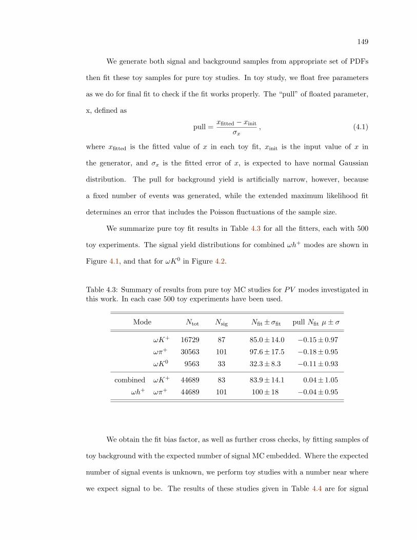
149

We generate both signal and background samples from appropriate set of PDFs

then fit these toy samples for pure toy studies. In toy study, we float free parameters

as we do for final fit to check if the fit works properly. The “pull” of floated parameter,

x, defined as

pull =xfitted − xinit

σx, (4.1)

where xfitted is the fitted value of x in each toy fit, xinit is the input value of x in

the generator, and σx is the fitted error of x, is expected to have normal Gaussian

distribution. The pull for background yield is artificially narrow, however, because

a fixed number of events was generated, while the extended maximum likelihood fit

determines an error that includes the Poisson fluctuations of the sample size.

We summarize pure toy fit results in Table 4.3 for all the fitters, each with 500

toy experiments. The signal yield distributions for combined ωh+ modes are shown in

Figure 4.1, and that for ωK0 in Figure 4.2.

Table 4.3: Summary of results from pure toy MC studies for PV modes investigated inthis work. In each case 500 toy experiments have been used.

Mode Ntot Nsig Nfit±σfit pull Nfit µ± σ

ωK+ 16729 87 85.0± 14.0 −0.15± 0.97

ωπ+ 30563 101 97.6± 17.5 −0.18± 0.95

ωK0 9563 33 32.3± 8.3 −0.11± 0.93

combined ωK+ 44689 83 83.9± 14.1 0.04± 1.05

ωh+ ωπ+ 44689 101 100± 18 −0.04± 0.95

We obtain the fit bias factor, as well as further cross checks, by fitting samples of

toy background with the expected number of signal MC embedded. Where the expected

number of signal events is unknown, we perform toy studies with a number near where

we expect signal to be. The results of these studies given in Table 4.4 are for signal

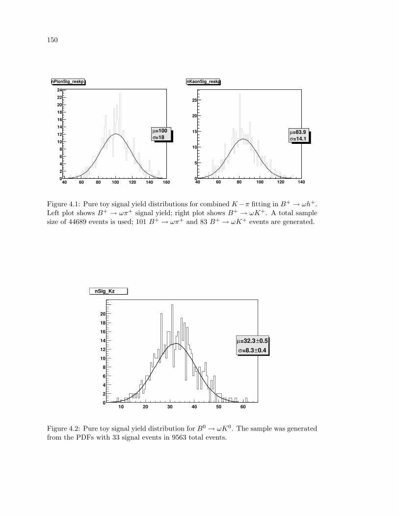
150

40 60 80 100 120 140 1600

2

4

6

8

10

12

14

16

18

20

22

24

nPionSig_reskp

=100µ=18σ

40 60 80 100 120 1400

5

10

15

20

25

nKaonSig_reskp

=83.9µ=14.1σ

Figure 4.1: Pure toy signal yield distributions for combined K−π fitting in B+ → ωh+.Left plot shows B+ → ωπ+ signal yield; right plot shows B+ → ωK+. A total samplesize of 44689 events is used; 101 B+ → ωπ+ and 83 B+ → ωK+ events are generated.

10 20 30 40 50 600

2

4

6

8

10

12

14

16

18

20

nSig_Kz

0.5±=32.3µ0.4±=8.3σ

Figure 4.2: Pure toy signal yield distribution for B0 → ωK0. The sample was generatedfrom the PDFs with 33 signal events in 9563 total events.

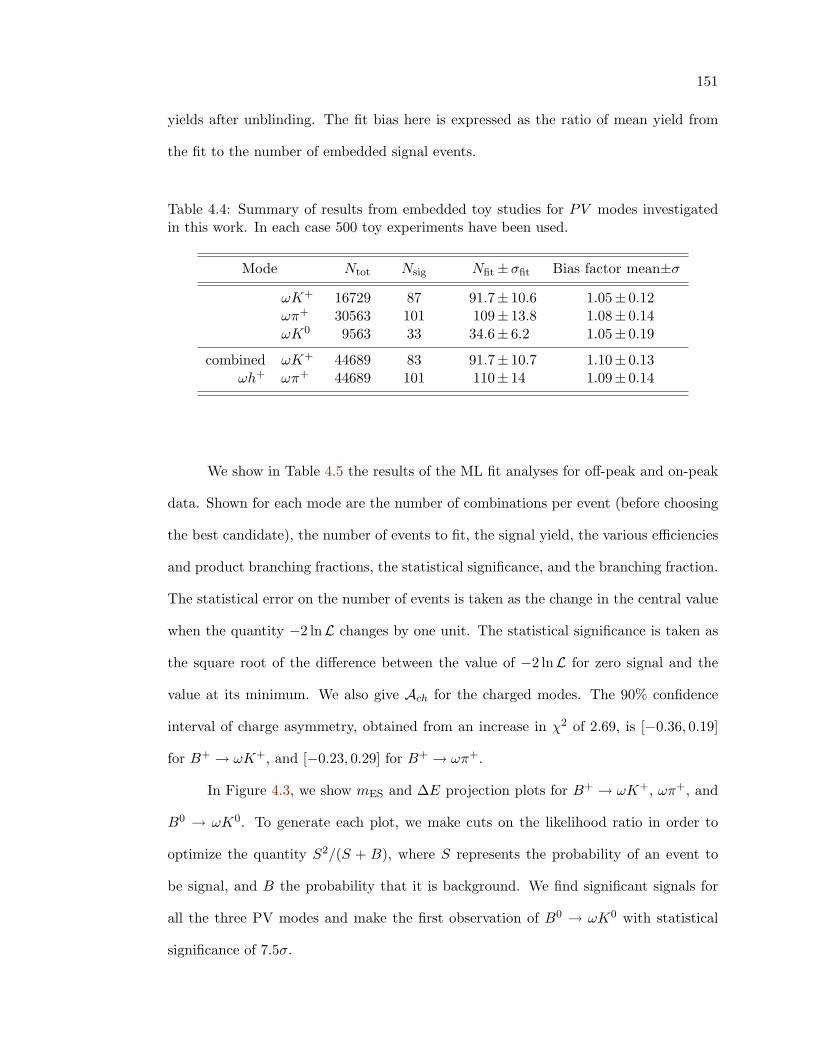
151

yields after unblinding. The fit bias here is expressed as the ratio of mean yield from

the fit to the number of embedded signal events.

Table 4.4: Summary of results from embedded toy studies for PV modes investigatedin this work. In each case 500 toy experiments have been used.

Mode Ntot Nsig Nfit±σfit Bias factor mean±σ

ωK+ 16729 87 91.7± 10.6 1.05± 0.12ωπ+ 30563 101 109± 13.8 1.08± 0.14ωK0 9563 33 34.6± 6.2 1.05± 0.19

combined ωK+ 44689 83 91.7± 10.7 1.10± 0.13ωh+ ωπ+ 44689 101 110± 14 1.09± 0.14

We show in Table 4.5 the results of the ML fit analyses for off-peak and on-peak

data. Shown for each mode are the number of combinations per event (before choosing

the best candidate), the number of events to fit, the signal yield, the various efficiencies

and product branching fractions, the statistical significance, and the branching fraction.

The statistical error on the number of events is taken as the change in the central value

when the quantity −2 lnL changes by one unit. The statistical significance is taken as

the square root of the difference between the value of −2 lnL for zero signal and the

value at its minimum. We also give Ach for the charged modes. The 90% confidence

interval of charge asymmetry, obtained from an increase in χ2 of 2.69, is [−0.36, 0.19]

for B+ → ωK+, and [−0.23, 0.29] for B+ → ωπ+.

In Figure 4.3, we show mES and ∆E projection plots for B+ → ωK+, ωπ+, and

B0 → ωK0. To generate each plot, we make cuts on the likelihood ratio in order to

optimize the quantity S2/(S + B), where S represents the probability of an event to

be signal, and B the probability that it is background. We find significant signals for

all the three PV modes and make the first observation of B0 → ωK0 with statistical

significance of 7.5σ.

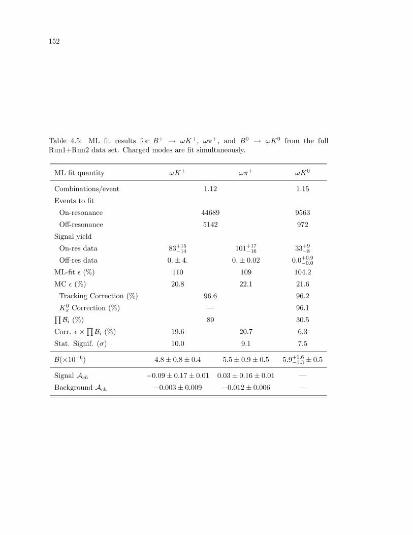
152

Table 4.5: ML fit results for B+ → ωK+, ωπ+, and B0 → ωK0 from the fullRun1+Run2 data set. Charged modes are fit simultaneously.

ML fit quantity ωK+ ωπ+ ωK0

Combinations/event 1.12 1.15

Events to fit

On-resonance 44689 9563

Off-resonance 5142 972

Signal yield

On-res data 83+15−14 101+17

−16 33+9−8

Off-res data 0.± 4. 0.± 0.02 0.0+0.9−0.0

ML-fit ε (%) 110 109 104.2

MC ε (%) 20.8 22.1 21.6

Tracking Correction (%) 96.6 96.2

K0S Correction (%) — 96.1∏Bi (%) 89 30.5

Corr. ε×∏Bi (%) 19.6 20.7 6.3

Stat. Signif. (σ) 10.0 9.1 7.5

B(×10−6) 4.8± 0.8± 0.4 5.5± 0.9± 0.5 5.9+1.6−1.3 ± 0.5

Signal Ach −0.09± 0.17± 0.01 0.03± 0.16± 0.01 —

Background Ach −0.003± 0.009 −0.012± 0.006 —

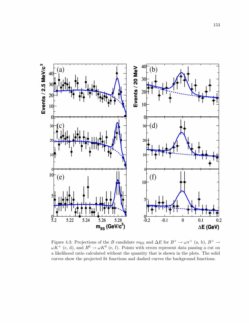
153

2E

ven

ts /

2.5

MeV

/c

0

10

20

30

40

2E

ven

ts /

2.5

MeV

/c

0

10

20

30

40

Eve

nts

/ 20

MeV

0

10

20

30

40

Eve

nts

/ 20

MeV

0

10

20

30

40

0

10

20

30

0

10

20

30

0

10

20

30

0

10

20

30

) 2 (GeV/cESm5.2 5.22 5.24 5.26 5.280

5

10

) 2 (GeV/cESm5.2 5.22 5.24 5.26 5.280

5

10

E (GeV)∆-0.2 -0.1 0 0.1 0.20

5

10

E (GeV)∆-0.2 -0.1 0 0.1 0.20

5

10

(a) (b)

(c) (d)

(e) (f)

Figure 4.3: Projections of the B candidate mES and ∆E for B+ → ωπ+ (a, b), B+ →ωK+ (c, d), and B0 → ωK0 (e, f). Points with errors represent data passing a cut ona likelihood ratio calculated without the quantity that is shown in the plots. The solidcurves show the projected fit functions and dashed curves the background functions.

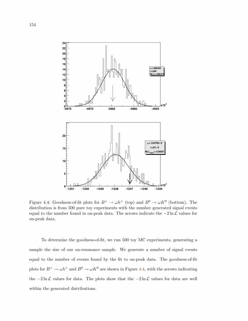
154

-4975 -4970 -4965 -4960 -4955

2x100

2

4

6

8

10

12

14

16

18

20

22

24

=-496462µ=266σ

NLL=-496474

-1251 -1250 -1249 -1248 -1247 -1246 -1245

2x100

5

10

15

20

5±=-124795µ

5±=91σ

=-124697dataNLL

Figure 4.4: Goodness-of-fit plots for B+ → ωh+ (top) and B0 → ωK0 (bottom). Thedistribution is from 500 pure toy experiments with the number generated signal eventsequal to the number found in on-peak data. The arrows indicate the −2 lnL values foron-peak data.

To determine the goodness-of-fit, we run 500 toy MC experiments, generating a

sample the size of our on-resonance sample. We generate a number of signal events

equal to the number of events found by the fit to on-peak data. The goodness-of-fit

plots for B+ → ωh+ and B0 → ωK0 are shown in Figure 4.4, with the arrows indicating

the −2 lnL values for data. The plots show that the −2 lnL values for data are well

within the generated distributions.

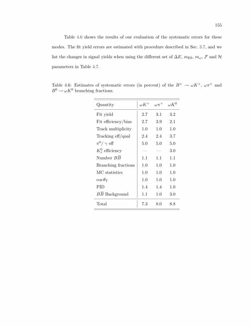
155

Table 4.6 shows the results of our evaluation of the systematic errors for these

modes. The fit yield errors are estimated with procedure described in Sec. 3.7, and we

list the changes in signal yields when using the different set of ∆E, mES, mω, F and H

parameters in Table 4.7.

Table 4.6: Estimates of systematic errors (in percent) of the B+ → ωK+, ωπ+ andB0 → ωK0 branching fractions.

Quantity ωK+ ωπ+ ωK0

Fit yield 2.7 3.1 3.2

Fit efficiency/bias 2.7 3.9 2.1

Track multiplicity 1.0 1.0 1.0

Tracking eff/qual 2.4 2.4 3.7

π0/ γ eff 5.0 5.0 5.0

K0S efficiency — — 3.0

Number BB 1.1 1.1 1.1

Branching fractions 1.0 1.0 1.0

MC statistics 1.0 1.0 1.0

cos θT 1.0 1.0 1.0

PID 1.4 1.4 1.0

BB Background 1.1 1.0 3.0

Total 7.3 8.0 8.8

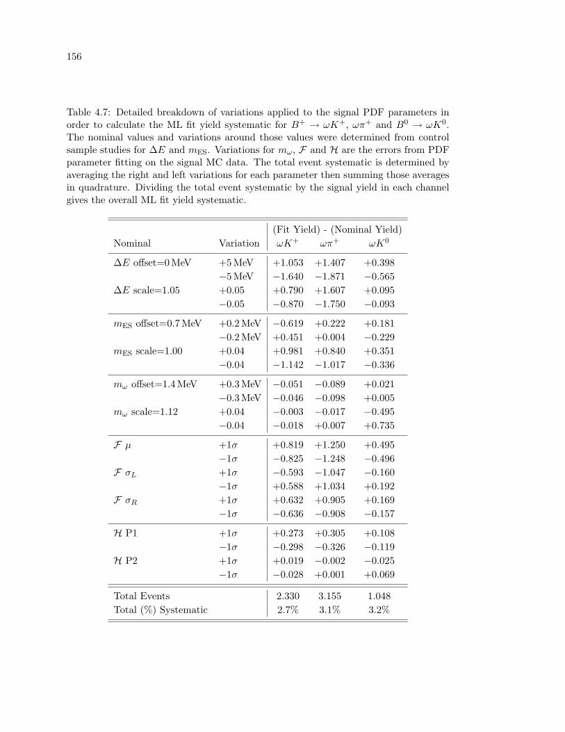
156

Table 4.7: Detailed breakdown of variations applied to the signal PDF parameters inorder to calculate the ML fit yield systematic for B+ → ωK+, ωπ+ and B0 → ωK0.The nominal values and variations around those values were determined from controlsample studies for ∆E and mES. Variations for mω, F and H are the errors from PDFparameter fitting on the signal MC data. The total event systematic is determined byaveraging the right and left variations for each parameter then summing those averagesin quadrature. Dividing the total event systematic by the signal yield in each channelgives the overall ML fit yield systematic.

(Fit Yield) - (Nominal Yield)Nominal Variation ωK+ ωπ+ ωK0

∆E offset=0 MeV +5 MeV +1.053 +1.407 +0.398−5 MeV −1.640 −1.871 −0.565

∆E scale=1.05 +0.05 +0.790 +1.607 +0.095−0.05 −0.870 −1.750 −0.093

mES offset=0.7 MeV +0.2 MeV −0.619 +0.222 +0.181−0.2 MeV +0.451 +0.004 −0.229

mES scale=1.00 +0.04 +0.981 +0.840 +0.351−0.04 −1.142 −1.017 −0.336

mω offset=1.4MeV +0.3 MeV −0.051 −0.089 +0.021−0.3 MeV −0.046 −0.098 +0.005

mω scale=1.12 +0.04 −0.003 −0.017 −0.495−0.04 −0.018 +0.007 +0.735

F µ +1σ +0.819 +1.250 +0.495−1σ −0.825 −1.248 −0.496

F σL +1σ −0.593 −1.047 −0.160−1σ +0.588 +1.034 +0.192

F σR +1σ +0.632 +0.905 +0.169−1σ −0.636 −0.908 −0.157

H P1 +1σ +0.273 +0.305 +0.108−1σ −0.298 −0.326 −0.119

H P2 +1σ +0.019 −0.002 −0.025−1σ −0.028 +0.001 +0.069

Total Events 2.330 3.155 1.048Total (%) Systematic 2.7% 3.1% 3.2%

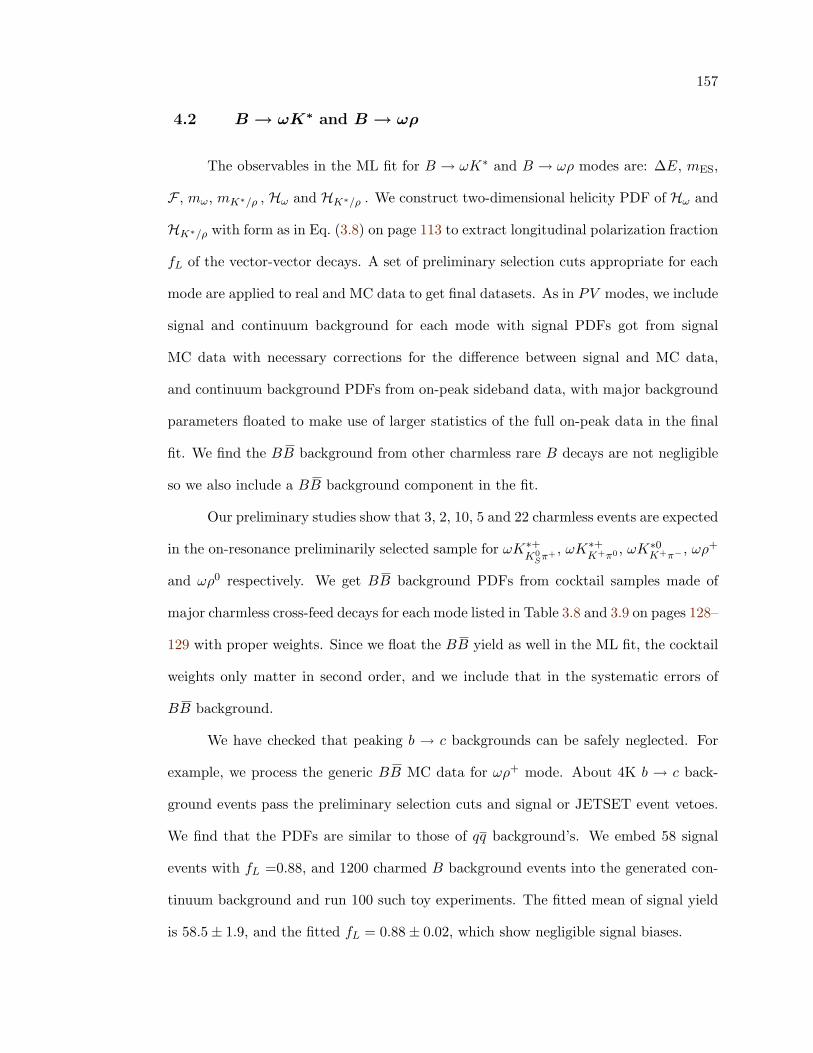
157

4.2 B → ωK∗ and B → ωρ

The observables in the ML fit for B → ωK∗ and B → ωρ modes are: ∆E, mES,

F , mω, mK∗/ρ , Hω and HK∗/ρ . We construct two-dimensional helicity PDF of Hω and

HK∗/ρ with form as in Eq. (3.8) on page 113 to extract longitudinal polarization fraction

fL of the vector-vector decays. A set of preliminary selection cuts appropriate for each

mode are applied to real and MC data to get final datasets. As in PV modes, we include

signal and continuum background for each mode with signal PDFs got from signal

MC data with necessary corrections for the difference between signal and MC data,

and continuum background PDFs from on-peak sideband data, with major background

parameters floated to make use of larger statistics of the full on-peak data in the final

fit. We find the BB background from other charmless rare B decays are not negligible

so we also include a BB background component in the fit.

Our preliminary studies show that 3, 2, 10, 5 and 22 charmless events are expected

in the on-resonance preliminarily selected sample for ωK∗+K0

Sπ+ , ωK∗+K+π0 , ωK∗0

K+π− , ωρ+

and ωρ0 respectively. We get BB background PDFs from cocktail samples made of

major charmless cross-feed decays for each mode listed in Table 3.8 and 3.9 on pages 128–

129 with proper weights. Since we float the BB yield as well in the ML fit, the cocktail

weights only matter in second order, and we include that in the systematic errors of

BB background.

We have checked that peaking b → c backgrounds can be safely neglected. For

example, we process the generic BB MC data for ωρ+ mode. About 4K b → c back-

ground events pass the preliminary selection cuts and signal or JETSET event vetoes.

We find that the PDFs are similar to those of qq background’s. We embed 58 signal

events with fL =0.88, and 1200 charmed B background events into the generated con-

tinuum background and run 100 such toy experiments. The fitted mean of signal yield

is 58.5± 1.9, and the fitted fL = 0.88± 0.02, which show negligible signal biases.

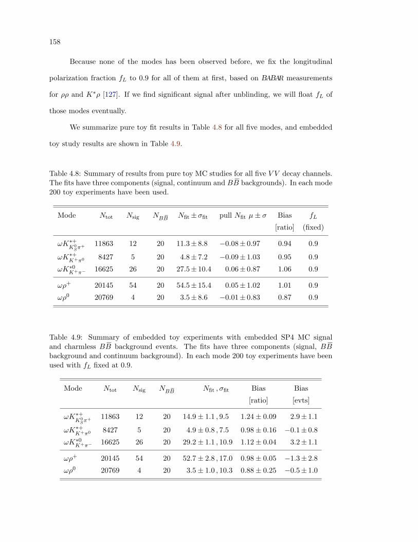
158

Because none of the modes has been observed before, we fix the longitudinal

polarization fraction fL to 0.9 for all of them at first, based on BABAR measurements

for ρρ and K∗ρ [127]. If we find significant signal after unblinding, we will float fL of

those modes eventually.

We summarize pure toy fit results in Table 4.8 for all five modes, and embedded

toy study results are shown in Table 4.9.

Table 4.8: Summary of results from pure toy MC studies for all five V V decay channels.The fits have three components (signal, continuum and BB backgrounds). In each mode200 toy experiments have been used.

Mode Ntot Nsig NBB Nfit±σfit pull Nfit µ± σ Bias fL

[ratio] (fixed)

ωK∗+K0

Sπ+ 11863 12 20 11.3± 8.8 −0.08± 0.97 0.94 0.9

ωK∗+K+π0 8427 5 20 4.8± 7.2 −0.09± 1.03 0.95 0.9

ωK∗0K+π− 16625 26 20 27.5± 10.4 0.06± 0.87 1.06 0.9

ωρ+ 20145 54 20 54.5± 15.4 0.05± 1.02 1.01 0.9

ωρ0 20769 4 20 3.5± 8.6 −0.01± 0.83 0.87 0.9

Table 4.9: Summary of embedded toy experiments with embedded SP4 MC signaland charmless BB background events. The fits have three components (signal, BBbackground and continuum background). In each mode 200 toy experiments have beenused with fL fixed at 0.9.

Mode Ntot Nsig NBB Nfit , σfit Bias Bias

[ratio] [evts]

ωK∗+K0

Sπ+ 11863 12 20 14.9± 1.1 , 9.5 1.24± 0.09 2.9± 1.1

ωK∗+K+π0 8427 5 20 4.9± 0.8 , 7.5 0.98± 0.16 −0.1± 0.8

ωK∗0K+π− 16625 26 20 29.2± 1.1 , 10.9 1.12± 0.04 3.2± 1.1

ωρ+ 20145 54 20 52.7± 2.8 , 17.0 0.98± 0.05 −1.3± 2.8

ωρ0 20769 4 20 3.5± 1.0 , 10.3 0.88± 0.25 −0.5± 1.0

159

From above toy experiment results, we estimate the sensitivity of on-peak sample

measurements. The upper limit estimation assumes that the measured signal yield is

zero and the statistical error is given by the average for zero embedded signal events.

So if we embed Nsig signal events and we get σtot as the sigma of the distribution, the

sigma for zero embedded signal events is estimated as σ =√σ2

tot −Nsig. The 90%

upper limit estimation is calculated as 1.28 σ/(ε×NBB). The central value sensitivity

is determined for assumed branching ratios of 9×10−6 for ωρ+ and 3.3×10−6 for the

other four modes. The expected results are summarized in table 4.10.

Table 4.10: Expected 90% upper limit (UL) with null observations and statistic sig-nificance with assumed branch fractions. The UL is determined using the preliminaryselection efficiencies listed in table 4.13 and 4.14. The CLEO results are from Ref. 51.

Mode σ 90% UL CLEO 90% UL Nsig Nfit±σfit signif

(B = 0) [10−6] [10−6] [σ]

ωK∗+K0

Sπ+ 8.4 4.4 109 10 10.5± 9.0 1.2

ωK∗+K+π0 4.5 3.0 129 7 8.3± 5.2 1.6

ωK∗0K+π− 11.6 2.1 23 22 25.1± 12.5 2.0

ωρ+ 13.7 4.4 61 50 57.8± 15.4 3.8

ωρ0 14.8 2.1 11 31 38.3± 15.8 2.4

After we unblind the yield-only fits, we find significant signal for B+ → ωρ+

mode, we then check the full fit with toy studies with fL floated in the range [0,1] for

B+ → ωρ+ mode before we unblind to get fL. Table 4.11 summarizes the pure toy

study results for different fL of ωρ+ mode. Table 4.12 summarizes the embedded toy

study results for different fL of ωρ+ mode.

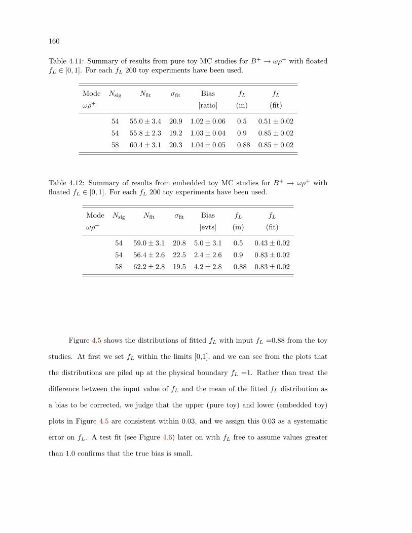
160

Table 4.11: Summary of results from pure toy MC studies for B+ → ωρ+ with floatedfL ∈ [0, 1]. For each fL 200 toy experiments have been used.

Mode Nsig Nfit σfit Bias fL fL

ωρ+ [ratio] (in) (fit)

54 55.0± 3.4 20.9 1.02± 0.06 0.5 0.51± 0.02

54 55.8± 2.3 19.2 1.03± 0.04 0.9 0.85± 0.02

58 60.4± 3.1 20.3 1.04± 0.05 0.88 0.85± 0.02

Table 4.12: Summary of results from embedded toy MC studies for B+ → ωρ+ withfloated fL ∈ [0, 1]. For each fL 200 toy experiments have been used.

Mode Nsig Nfit σfit Bias fL fL

ωρ+ [evts] (in) (fit)

54 59.0± 3.1 20.8 5.0± 3.1 0.5 0.43± 0.02

54 56.4± 2.6 22.5 2.4± 2.6 0.9 0.83± 0.02

58 62.2± 2.8 19.5 4.2± 2.8 0.88 0.83± 0.02

Figure 4.5 shows the distributions of fitted fL with input fL =0.88 from the toy

studies. At first we set fL within the limits [0,1], and we can see from the plots that

the distributions are piled up at the physical boundary fL =1. Rather than treat the

difference between the input value of fL and the mean of the fitted fL distribution as

a bias to be corrected, we judge that the upper (pure toy) and lower (embedded toy)

plots in Figure 4.5 are consistent within 0.03, and we assign this 0.03 as a systematic

error on fL. A test fit (see Figure 4.6) later on with fL free to assume values greater

than 1.0 confirms that the true bias is small.

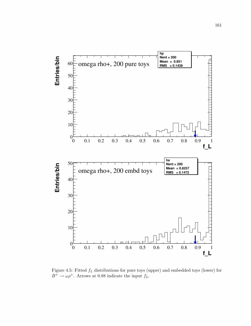
161

f_L0 0.1 0.2 0.3 0.4 0.5 0.6 0.7 0.8 0.9 1

Ent

ries

/bin

0

10

20

30

40

50

60

hpNent = 200 Mean = 0.851RMS = 0.1438omega rho+, 200 pure toys

hpNent = 200 Mean = 0.851RMS = 0.1438

f_L0 0.1 0.2 0.3 0.4 0.5 0.6 0.7 0.8 0.9 1

Ent

ries

/bin

0

10

20

30

40

50heNent = 200 Mean = 0.8257RMS = 0.1472omega rho+, 200 embd toys

heNent = 200 Mean = 0.8257RMS = 0.1472

Figure 4.5: Fitted fL distributions for pure toys (upper) and embedded toys (lower) forB+ → ωρ+. Arrows at 0.88 indicate the input fL.

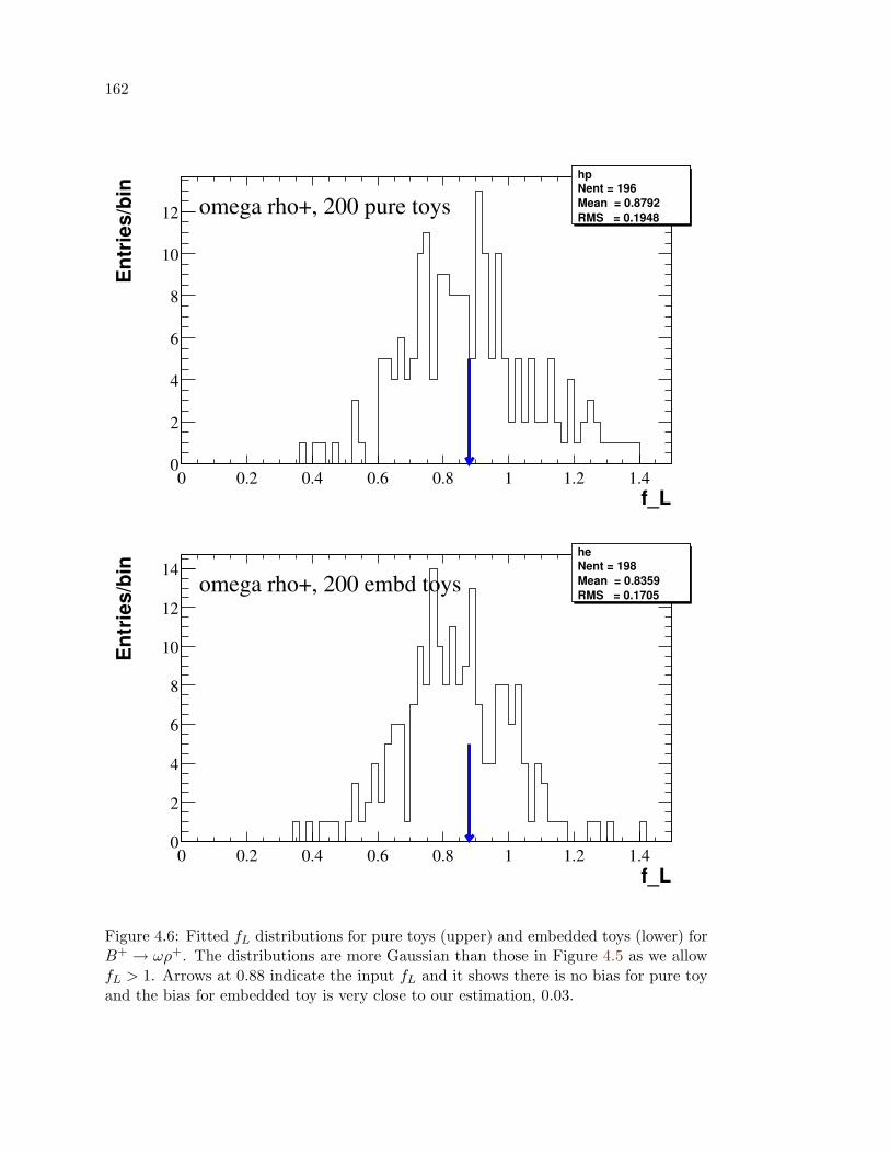
162

f_L0 0.2 0.4 0.6 0.8 1 1.2 1.4

Ent

ries

/bin

0

2

4

6

8

10

12

hpNent = 196 Mean = 0.8792RMS = 0.1948

omega rho+, 200 pure toys

hpNent = 196 Mean = 0.8792RMS = 0.1948

f_L0 0.2 0.4 0.6 0.8 1 1.2 1.4

Ent

ries

/bin

0

2

4

6

8

10

12

14heNent = 198 Mean = 0.8359RMS = 0.1705

omega rho+, 200 embd toys

heNent = 198 Mean = 0.8359RMS = 0.1705

Figure 4.6: Fitted fL distributions for pure toys (upper) and embedded toys (lower) forB+ → ωρ+. The distributions are more Gaussian than those in Figure 4.5 as we allowfL > 1. Arrows at 0.88 indicate the input fL and it shows there is no bias for pure toyand the bias for embedded toy is very close to our estimation, 0.03.

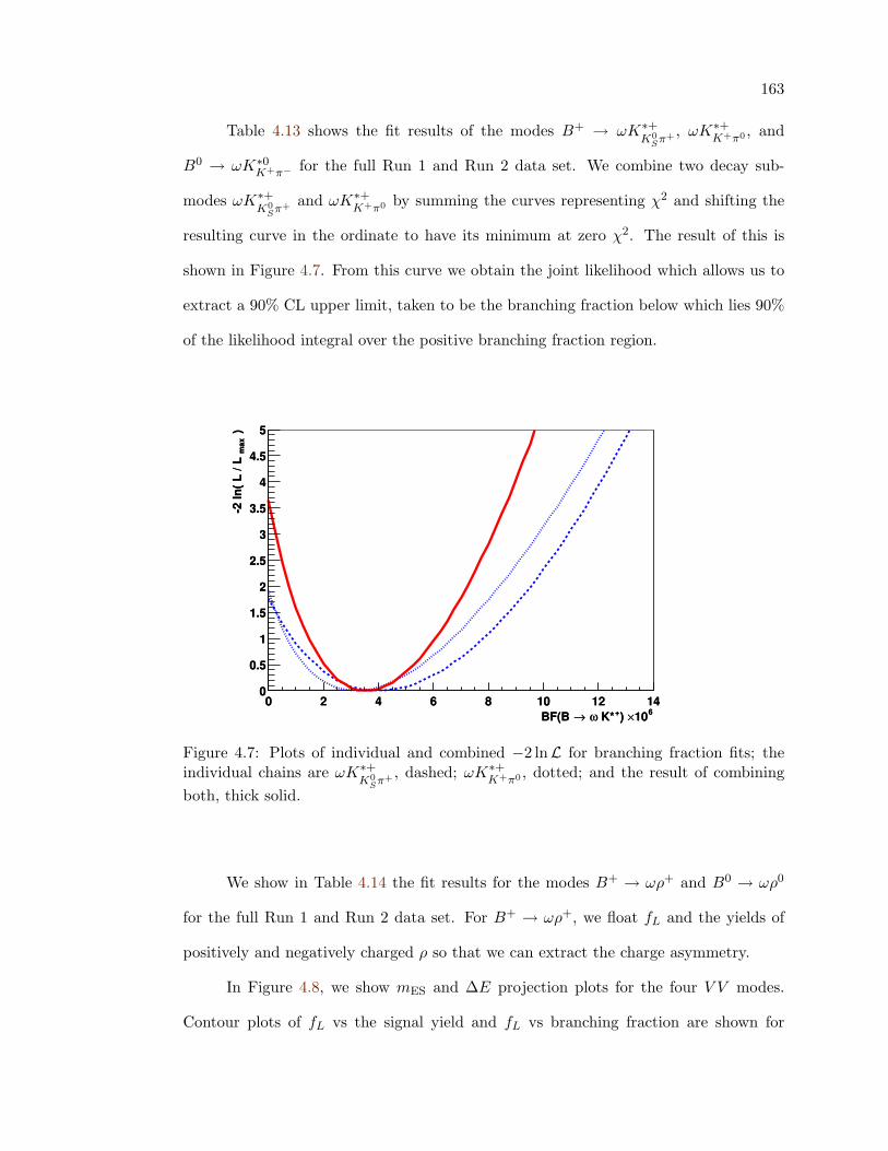
163

Table 4.13 shows the fit results of the modes B+ → ωK∗+K0

Sπ+ , ωK∗+K+π0 , and

B0 → ωK∗0K+π− for the full Run 1 and Run 2 data set. We combine two decay sub-

modes ωK∗+K0

Sπ+ and ωK∗+K+π0 by summing the curves representing χ2 and shifting the

resulting curve in the ordinate to have its minimum at zero χ2. The result of this is

shown in Figure 4.7. From this curve we obtain the joint likelihood which allows us to

extract a 90% CL upper limit, taken to be the branching fraction below which lies 90%

of the likelihood integral over the positive branching fraction region.

610×) + K*ω →BF(B 0 2 4 6 8 10 12 14

) m

ax-2

ln( L

/ L

0

0.5

1

1.5

2

2.5

3

3.5

4

4.5

5

610×) + K*ω →BF(B 0 2 4 6 8 10 12 14

) m

ax-2

ln( L

/ L

0

0.5

1

1.5

2

2.5

3

3.5

4

4.5

5

Figure 4.7: Plots of individual and combined −2 lnL for branching fraction fits; theindividual chains are ωK∗+

K0Sπ+ , dashed; ωK∗+

K+π0 , dotted; and the result of combiningboth, thick solid.

We show in Table 4.14 the fit results for the modes B+ → ωρ+ and B0 → ωρ0

for the full Run 1 and Run 2 data set. For B+ → ωρ+, we float fL and the yields of

positively and negatively charged ρ so that we can extract the charge asymmetry.

In Figure 4.8, we show mES and ∆E projection plots for the four V V modes.

Contour plots of fL vs the signal yield and fL vs branching fraction are shown for

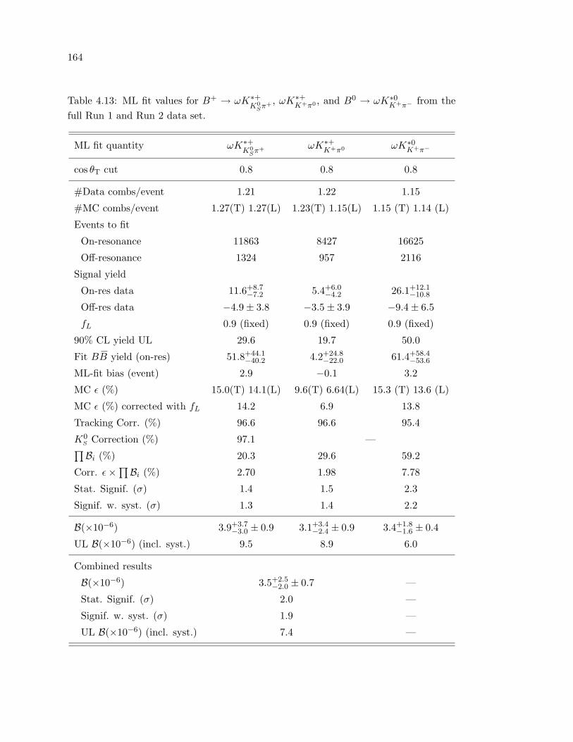
164

Table 4.13: ML fit values for B+ → ωK∗+K0

Sπ+ , ωK∗+K+π0 , and B0 → ωK∗0

K+π− from thefull Run 1 and Run 2 data set.

ML fit quantity ωK∗+K0


K+π−

cos θT cut 0.8 0.8 0.8

#Data combs/event 1.21 1.22 1.15

#MC combs/event 1.27(T) 1.27(L) 1.23(T) 1.15(L) 1.15 (T) 1.14 (L)

Events to fit

On-resonance 11863 8427 16625

Off-resonance 1324 957 2116

Signal yield

On-res data 11.6+8.7−7.2 5.4+6.0

−4.2 26.1+12.1−10.8

Off-res data −4.9± 3.8 −3.5± 3.9 −9.4± 6.5

fL 0.9 (fixed) 0.9 (fixed) 0.9 (fixed)

90% CL yield UL 29.6 19.7 50.0

Fit BB yield (on-res) 51.8+44.1−40.2 4.2+24.8

−22.0 61.4+58.4−53.6

ML-fit bias (event) 2.9 −0.1 3.2

MC ε (%) 15.0(T) 14.1(L) 9.6(T) 6.64(L) 15.3 (T) 13.6 (L)

MC ε (%) corrected with fL 14.2 6.9 13.8

Tracking Corr. (%) 96.6 96.6 95.4

K0S Correction (%) 97.1 —∏Bi (%) 20.3 29.6 59.2

Corr. ε×∏Bi (%) 2.70 1.98 7.78

Stat. Signif. (σ) 1.4 1.5 2.3

Signif. w. syst. (σ) 1.3 1.4 2.2

B(×10−6) 3.9+3.7−3.0 ± 0.9 3.1+3.4

−2.4 ± 0.9 3.4+1.8−1.6 ± 0.4

UL B(×10−6) (incl. syst.) 9.5 8.9 6.0

Combined results

B(×10−6) 3.5+2.5−2.0 ± 0.7 —

Stat. Signif. (σ) 2.0 —

Signif. w. syst. (σ) 1.9 —

UL B(×10−6) (incl. syst.) 7.4 —

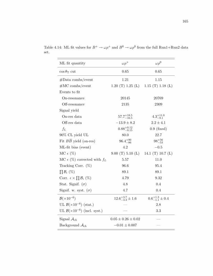
165

Table 4.14: ML fit values for B+ → ωρ+ and B0 → ωρ0 from the full Run1+Run2 dataset.

ML fit quantity ωρ+ ωρ0

cos θT cut 0.65 0.65

#Data combs/event 1.21 1.15

#MC combs/event 1.20 (T) 1.25 (L) 1.15 (T) 1.18 (L)

Events to fit

On-resonance 20145 20769

Off-resonance 2135 2309

Signal yield

On-res data 57.7+18.5−16.5 4.3+11.0

−9.1

Off-res data −13.9± 8.2 2.2± 4.1

fL 0.88+0.12−0.15 0.9 (fixed)

90% CL yield UL 80.0 22.7

Fit BB yield (on-res) 96.4+90−86 98+56

−53

ML-fit bias (event) 4.2 −0.5

MC ε (%) 9.00 (T) 5.10 (L) 14.1 (T) 10.7 (L)

MC ε (%) corrected with fL 5.57 11.0

Tracking Corr. (%) 96.6 95.4∏Bi (%) 89.1 89.1

Corr. ε×∏Bi (%) 4.79 9.32

Stat. Signif. (σ) 4.8 0.4

Signif. w. syst. (σ) 4.7 0.4

B(×10−6) 12.6+3.7−3.3 ± 1.6 0.6+1.3

−1.1 ± 0.4

UL B(×10−6) (stat.) — 2.8

UL B(×10−6) (incl. syst.) — 3.3

Signal Ach 0.05± 0.26± 0.02 —

Background Ach −0.01± 0.007 —

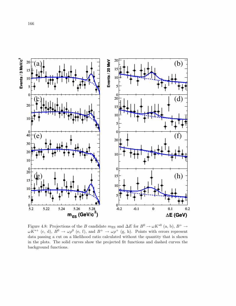
1662

Eve

nts

/ 3 M

eV/c

0

5

10

15

20

2E

vent

s / 3

MeV

/c

0

5

10

15

20

Eve

nts

/ 20

MeV

0

5

10

15

20

Eve

nts

/ 20

MeV

0

5

10

15

20

0

10

20

0

10

20

0

5

10

15

20

0

5

10

15

20

0

10

20

30

40

0

10

20

30

40

0

10

20

0

10

20

) 2 (GeV/cESm5.2 5.22 5.24 5.26 5.280

5

10

15

20

) 2 (GeV/cESm5.2 5.22 5.24 5.26 5.280

5

10

15

20

E (GeV)∆-0.2 -0.1 0 0.1 0.20

5

10

15

E (GeV)∆-0.2 -0.1 0 0.1 0.20

5

10

15

(a) (b)

(c) (d)

(e) (f)

(g) (h)

Figure 4.8: Projections of the B candidate mES and ∆E for B0 → ωK∗0 (a, b), B+ →ωK∗+ (c, d), B0 → ωρ0 (e, f), and B+ → ωρ+ (g, h). Points with errors representdata passing a cut on a likelihood ratio calculated without the quantity that is shownin the plots. The solid curves show the projected fit functions and dashed curves thebackground functions.

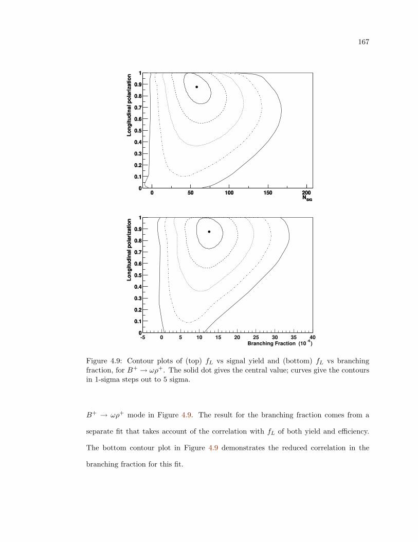
167

SIGN0 50 100 150 200

Long

itudi

nal p

olar

izat

ion

0

0.1

0.2

0.3

0.4

0.5

0.6

0.7

0.8

0.9

1

SIGN0 50 100 150 200

Long

itudi

nal p

olar

izat

ion

0

0.1

0.2

0.3

0.4

0.5

0.6

0.7

0.8

0.9

1

Long

itudi

nal p

olar

izat

ion

0

0.1

0.2

0.3

0.4

0.5

0.6

0.7

0.8

0.9

1

Long

itudi

nal p

olar

izat

ion

0

0.1

0.2

0.3

0.4

0.5

0.6

0.7

0.8

0.9

1

)-6Branching Fraction (10-5 0 5 10 15 20 25 30 35 40

Figure 4.9: Contour plots of (top) fL vs signal yield and (bottom) fL vs branchingfraction, for B+ → ωρ+. The solid dot gives the central value; curves give the contoursin 1-sigma steps out to 5 sigma.

B+ → ωρ+ mode in Figure 4.9. The result for the branching fraction comes from a

separate fit that takes account of the correlation with fL of both yield and efficiency.

The bottom contour plot in Figure 4.9 demonstrates the reduced correlation in the

branching fraction for this fit.

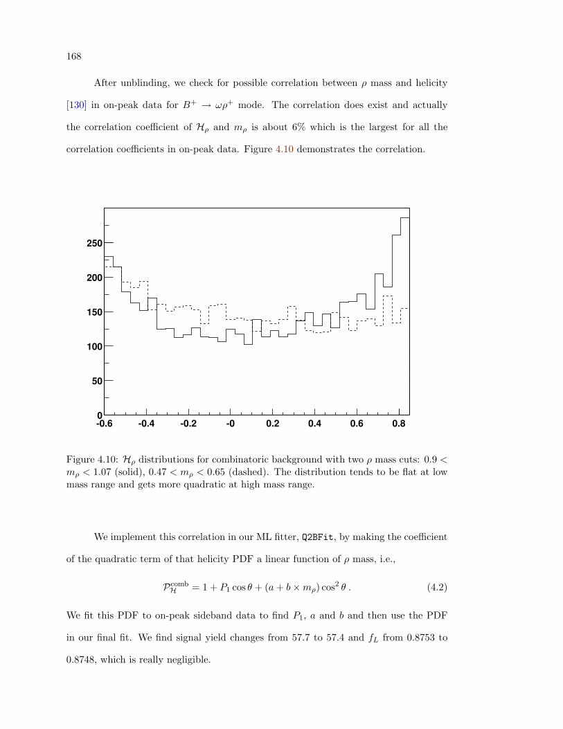
168

After unblinding, we check for possible correlation between ρ mass and helicity

[130] in on-peak data for B+ → ωρ+ mode. The correlation does exist and actually

the correlation coefficient of Hρ and mρ is about 6% which is the largest for all the

correlation coefficients in on-peak data. Figure 4.10 demonstrates the correlation.

-0.6 -0.4 -0.2 -0 0.2 0.4 0.6 0.80

50

100

150

200

250

Figure 4.10: Hρ distributions for combinatoric background with two ρ mass cuts: 0.9 <mρ < 1.07 (solid), 0.47 < mρ < 0.65 (dashed). The distribution tends to be flat at lowmass range and gets more quadratic at high mass range.

We implement this correlation in our ML fitter, Q2BFit, by making the coefficient

of the quadratic term of that helicity PDF a linear function of ρ mass, i.e.,

PcombH = 1 + P1 cos θ + (a+ b×mρ) cos2 θ . (4.2)

We fit this PDF to on-peak sideband data to find P1, a and b and then use the PDF

in our final fit. We find signal yield changes from 57.7 to 57.4 and fL from 0.8753 to

0.8748, which is really negligible.

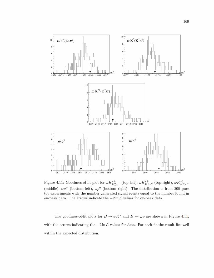
169

-1674 -1673 -1672 -1671 -1670 -1669 -1668 -1667

2x100

2

4

6

8

10 )+π(Ks* Kω

-1177 -1176 -1175 -1174 -1173 -1172

2x100

2

4

6

8

10

)0π+(K* Kω

-2719 -2718 -2717 -2716 -2715 -2714 -2713 -2712 -2711

2x100

2

4

6

8

10

)-π+(K*0 Kω

-2877 -2876 -2875 -2874 -2873 -2872 -2871 -2870

2x100

1

2

3

4

5

6

7

+ρ ω

-2948 -2946 -2944 -2942 -2940

2x100

1

2

3

4

5

6

7

8

9

0ρ ω

Figure 4.11: Goodness-of-fit plot for ωK∗+K0

Sπ+ (top left), ωK∗+K+π0 (top right), ωK∗0

K+π−

(middle), ωρ+ (bottom left), ωρ0 (bottom right). The distribution is from 200 puretoy experiments with the number generated signal events equal to the number found inon-peak data. The arrows indicate the −2 lnL values for on-peak data.

The goodness-of-fit plots for B → ωK∗ and B → ωρ are shown in Figure 4.11,

with the arrows indicating the −2 lnL values for data. For each fit the result lies well

within the expected distribution.

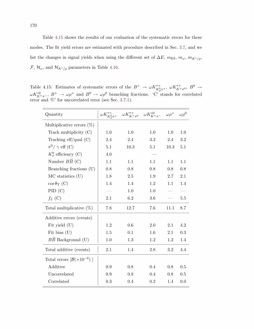
170

Table 4.15 shows the results of our evaluation of the systematic errors for these

modes. The fit yield errors are estimated with procedure described in Sec. 3.7, and we

list the changes in signal yields when using the different set of ∆E, mES, mω, mK∗/ρ,

F , Hω, and HK∗/ρ parameters in Table 4.16.

Table 4.15: Estimates of systematic errors of the B+ → ωK∗+K0

Sπ+ , ωK∗+K+π0 , B0 →

ωK∗0K+π− , B+ → ωρ+ and B0 → ωρ0 branching fractions. ‘C’ stands for correlated

error and ‘U’ for uncorrelated error (see Sec. 3.7.1).

Quantity ωK∗+K0


K+π− ωρ+ ωρ0

Multiplicative errors (%)

Track multiplicity (C) 1.0 1.0 1.0 1.0 1.0

Tracking eff/qual (C) 2.4 2.4 3.2 2.4 3.2

π0/ γ eff (C) 5.1 10.3 5.1 10.3 5.1

K0S efficiency (C) 4.0 —

Number BB (C) 1.1 1.1 1.1 1.1 1.1

Branching fractions (U) 0.8 0.8 0.8 0.8 0.8

MC statistics (U) 1.8 2.5 1.9 2.7 2.1

cos θT (C) 1.4 1.4 1.2 1.1 1.4

PID (C) — 1.0 1.0 — —

fL (C) 2.1 6.2 3.6 — 5.5

Total multiplicative (%) 7.8 12.7 7.6 11.1 8.7

Additive errors (events)

Fit yield (U) 1.2 0.6 2.0 2.1 4.2

Fit bias (U) 1.5 0.1 1.6 2.1 0.3

BB Background (U) 1.0 1.3 1.2 1.2 1.4

Total additive (events) 2.1 1.4 2.8 3.2 4.4

Total errors [B(×10−6) ]

Additive 0.9 0.8 0.4 0.8 0.5

Uncorrelated 0.9 0.8 0.4 0.8 0.5

Correlated 0.3 0.4 0.2 1.4 0.0

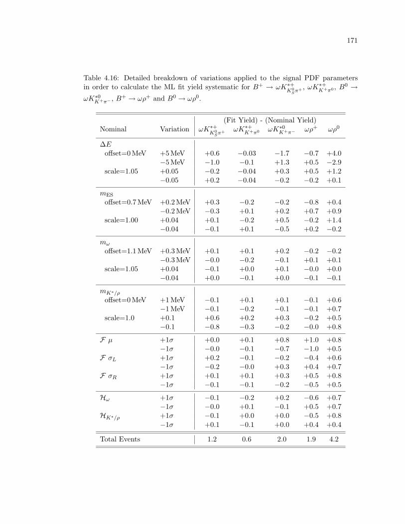
171

Table 4.16: Detailed breakdown of variations applied to the signal PDF parametersin order to calculate the ML fit yield systematic for B+ → ωK∗+

K0Sπ+ , ωK∗+

K+π0 , B0 →ωK∗0

K+π− , B+ → ωρ+ and B0 → ωρ0.

(Fit Yield) - (Nominal Yield)Nominal Variation ωK∗+

K0Sπ+ ωK∗+

K+π0 ωK∗0K+π− ωρ+ ωρ0

∆Eoffset=0 MeV +5 MeV +0.6 −0.03 −1.7 −0.7 +4.0

−5 MeV −1.0 −0.1 +1.3 +0.5 −2.9scale=1.05 +0.05 −0.2 −0.04 +0.3 +0.5 +1.2

−0.05 +0.2 −0.04 −0.2 −0.2 +0.1

mES

offset=0.7 MeV +0.2 MeV +0.3 −0.2 −0.2 −0.8 +0.4−0.2 MeV −0.3 +0.1 +0.2 +0.7 +0.9

scale=1.00 +0.04 +0.1 −0.2 +0.5 −0.2 +1.4−0.04 −0.1 +0.1 −0.5 +0.2 −0.2

mω

offset=1.1MeV +0.3 MeV +0.1 +0.1 +0.2 −0.2 −0.2−0.3 MeV −0.0 −0.2 −0.1 +0.1 +0.1

scale=1.05 +0.04 −0.1 +0.0 +0.1 −0.0 +0.0−0.04 +0.0 −0.1 +0.0 −0.1 −0.1

mK∗/ρ

offset=0 MeV +1 MeV −0.1 +0.1 +0.1 −0.1 +0.6−1 MeV −0.1 −0.2 −0.1 −0.1 +0.7

scale=1.0 +0.1 +0.6 +0.2 +0.3 −0.2 +0.5−0.1 −0.8 −0.3 −0.2 −0.0 +0.8

F µ +1σ +0.0 +0.1 +0.8 +1.0 +0.8−1σ −0.0 −0.1 −0.7 −1.0 +0.5

F σL +1σ +0.2 −0.1 −0.2 −0.4 +0.6−1σ −0.2 −0.0 +0.3 +0.4 +0.7

F σR +1σ +0.1 +0.1 +0.3 +0.5 +0.8−1σ −0.1 −0.1 −0.2 −0.5 +0.5

Hω +1σ −0.1 −0.2 +0.2 −0.6 +0.7−1σ −0.0 +0.1 −0.1 +0.5 +0.7

HK∗/ρ +1σ −0.1 +0.0 +0.0 −0.5 +0.8−1σ +0.1 −0.1 +0.0 +0.4 +0.4

Total Events 1.2 0.6 2.0 1.9 4.2

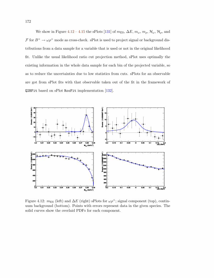
172

We show in Figure 4.12 – 4.15 the sPlots [131] of mES, ∆E, mω, mρ, Hω, Hρ, and

F for B+ → ωρ+ mode as cross-check. sPlot is used to project signal or background dis-

tributions from a data sample for a variable that is used or not in the original likelihood

fit. Unlike the usual likelihood ratio cut projection method, sPlot uses optimally the

existing information in the whole data sample for each bin of the projected variable, so

as to reduce the uncertainties due to low statistics from cuts. sPlots for an observable

are got from sPlot fits with that observable taken out of the fit in the framework of

Q2BFit based on sPlot RooFit implementation [132].

)2 (GeV/cESM5.2 5.21 5.22 5.23 5.24 5.25 5.26 5.27 5.28 5.29

Eve

nts

/ ( 0

.004

5 G

eV )

-10

0

10

20

30

40

50

)2 (GeV/cESM5.2 5.21 5.22 5.23 5.24 5.25 5.26 5.27 5.28 5.29

Eve

nts

/ ( 0

.004

5 G

eV )

-10

0

10

20

30

40

50

)2 (GeV/cESM5.2 5.21 5.22 5.23 5.24 5.25 5.26 5.27 5.28 5.29

Eve

nts

/ ( 0

.004

5 G

eV )

0

200

400

600

800

1000

1200

)2 (GeV/cESM5.2 5.21 5.22 5.23 5.24 5.25 5.26 5.27 5.28 5.29

Eve

nts

/ ( 0

.004

5 G

eV )

0

200

400

600

800

1000

1200

(E) (GeV)∆-0.2 -0.15 -0.1 -0.05 -0 0.05 0.1 0.15 0.2

Eve

nts

/ ( 0

.026

6667

GeV

)

-5

0

5

10

15

(E) (GeV)∆-0.2 -0.15 -0.1 -0.05 -0 0.05 0.1 0.15 0.2

Eve

nts

/ ( 0

.026

6667

GeV

)

-5

0

5

10

15

(E) (GeV)∆-0.2 -0.15 -0.1 -0.05 -0 0.05 0.1 0.15 0.2

Eve

nts

/ ( 0

.026

6667

GeV

)

0

200

400

600

800

1000

1200

1400

1600

1800

(E) (GeV)∆-0.2 -0.15 -0.1 -0.05 -0 0.05 0.1 0.15 0.2

Eve

nts

/ ( 0

.026

6667

GeV

)

0

200

400

600

800

1000

1200

1400

1600

1800

Figure 4.12: mES (left) and ∆E (right) sPlots for ωρ+; signal component (top), contin-uum background (bottom). Points with errors represent data in the given species. Thesolid curves show the overlaid PDFs for each component.

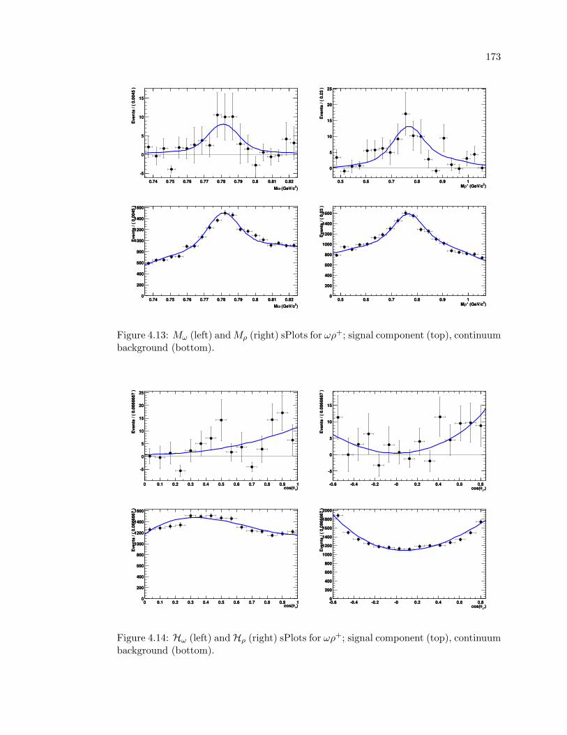
173

)2 (GeV/cωM0.74 0.75 0.76 0.77 0.78 0.79 0.8 0.81 0.82

Eve

nts

/ ( 0

.004

5 )

-5

0

5

10

15

)2 (GeV/cωM0.74 0.75 0.76 0.77 0.78 0.79 0.8 0.81 0.82

Eve

nts

/ ( 0

.004

5 )

-5

0

5

10

15

)2 (GeV/cωM0.74 0.75 0.76 0.77 0.78 0.79 0.8 0.81 0.82

Eve

nts

/ ( 0

.004

5 )

0

200

400

600

800

1000

1200

1400

1600

)2 (GeV/cωM0.74 0.75 0.76 0.77 0.78 0.79 0.8 0.81 0.82

Eve

nts

/ ( 0

.004

5 )

0

200

400

600

800

1000

1200

1400

1600

)2 (GeV/c+ρM0.5 0.6 0.7 0.8 0.9 1

Eve

nts

/ ( 0

.03

)

0

5

10

15

20

25

)2 (GeV/c+ρM0.5 0.6 0.7 0.8 0.9 1

Eve

nts

/ ( 0

.03

)

0

5

10

15

20

25

)2 (GeV/c+ρM0.5 0.6 0.7 0.8 0.9 1

Eve

nts

/ ( 0

.03

)

0

200

400

600

800

1000

1200

1400

1600

)2 (GeV/c+ρM0.5 0.6 0.7 0.8 0.9 1

Eve

nts

/ ( 0

.03

)

0

200

400

600

800

1000

1200

1400

1600

Figure 4.13: Mω (left) andMρ (right) sPlots for ωρ+; signal component (top), continuumbackground (bottom).

)ωθcos(0 0.1 0.2 0.3 0.4 0.5 0.6 0.7 0.8 0.9 1

Eve

nts

/ ( 0

.066

6667

)

-5

0

5

10

15

20

25

)ωθcos(0 0.1 0.2 0.3 0.4 0.5 0.6 0.7 0.8 0.9 1

Eve

nts

/ ( 0

.066

6667

)

-5

0

5

10

15

20

25

)ωθcos(0 0.1 0.2 0.3 0.4 0.5 0.6 0.7 0.8 0.9 1

Eve

nts

/ ( 0

.066

6667

)

0

200

400

600

800

1000

1200

1400

1600

)ωθcos(0 0.1 0.2 0.3 0.4 0.5 0.6 0.7 0.8 0.9 1

Eve

nts

/ ( 0

.066

6667

)

0

200

400

600

800

1000

1200

1400

1600

)+ρθcos(-0.6 -0.4 -0.2 -0 0.2 0.4 0.6 0.8

Eve

nts

/ ( 0

.096

6667

)

-5

0

5

10

15

)+ρθcos(-0.6 -0.4 -0.2 -0 0.2 0.4 0.6 0.8

Eve

nts

/ ( 0

.096

6667

)

-5

0

5

10

15

)+ρθcos(-0.6 -0.4 -0.2 -0 0.2 0.4 0.6 0.8

Eve

nts

/ ( 0

.096

6667

)

0

200

400

600

800

1000

1200

1400

1600

1800

2000

)+ρθcos(-0.6 -0.4 -0.2 -0 0.2 0.4 0.6 0.8

Eve

nts

/ ( 0

.096

6667

)

0

200

400

600

800

1000

1200

1400

1600

1800

2000

Figure 4.14: Hω (left) andHρ (right) sPlots for ωρ+; signal component (top), continuumbackground (bottom).

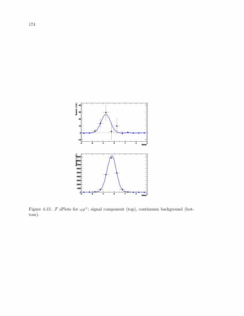
174

fisher -3 -2 -1 0 1 2 3

Eve

nts

/ ( 0

.5 )

-10

0

10

20

30

40

fisher -3 -2 -1 0 1 2 3

Eve

nts

/ ( 0

.5 )

-10

0

10

20

30

40

fisher -3 -2 -1 0 1 2 3

Eve

nts

/ ( 0

.5 )

0

1000

2000

3000

4000

5000

6000

7000

8000

9000

fisher -3 -2 -1 0 1 2 3

Eve

nts

/ ( 0

.5 )

0

1000

2000

3000

4000

5000

6000

7000

8000

9000

Figure 4.15: F sPlots for ωρ+; signal component (top), continuum background (bot-tom).

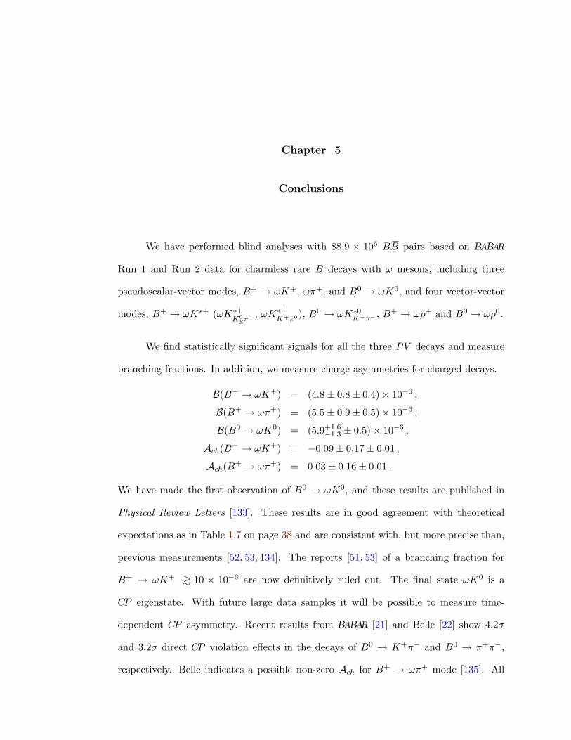
Chapter 5

Conclusions

We have performed blind analyses with 88.9 × 106 BB pairs based on BABAR

Run 1 and Run 2 data for charmless rare B decays with ω mesons, including three

pseudoscalar-vector modes, B+ → ωK+, ωπ+, and B0 → ωK0, and four vector-vector

modes, B+ → ωK∗+ (ωK∗+K0

Sπ+ , ωK∗+K+π0), B0 → ωK∗0

K+π− , B+ → ωρ+ and B0 → ωρ0.

We find statistically significant signals for all the three PV decays and measure

branching fractions. In addition, we measure charge asymmetries for charged decays.

B(B+ → ωK+) = (4.8± 0.8± 0.4)× 10−6 ,

B(B+ → ωπ+) = (5.5± 0.9± 0.5)× 10−6 ,

B(B0 → ωK0) = (5.9+1.6−1.3 ± 0.5)× 10−6 ,

Ach(B+ → ωK+) = −0.09± 0.17± 0.01 ,

Ach(B+ → ωπ+) = 0.03± 0.16± 0.01 .

We have made the first observation of B0 → ωK0, and these results are published in

Physical Review Letters [133]. These results are in good agreement with theoretical

expectations as in Table 1.7 on page 38 and are consistent with, but more precise than,

previous measurements [52, 53, 134]. The reports [51, 53] of a branching fraction for

B+ → ωK+ >∼ 10 × 10−6 are now definitively ruled out. The final state ωK0 is a

CP eigenstate. With future large data samples it will be possible to measure time-

dependent CP asymmetry. Recent results from BABAR [21] and Belle [22] show 4.2σ

and 3.2σ direct CP violation effects in the decays of B0 → K+π− and B0 → π+π−,

respectively. Belle indicates a possible non-zero Ach for B+ → ωπ+ mode [135]. All

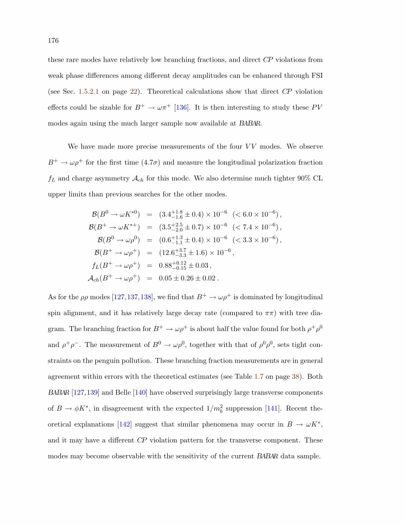
176

these rare modes have relatively low branching fractions, and direct CP violations from

weak phase differences among different decay amplitudes can be enhanced through FSI

(see Sec. 1.5.2.1 on page 22). Theoretical calculations show that direct CP violation

effects could be sizable for B+ → ωπ+ [136]. It is then interesting to study these PV

modes again using the much larger sample now available at BABAR.

We have made more precise measurements of the four V V modes. We observe

B+ → ωρ+ for the first time (4.7σ) and measure the longitudinal polarization fraction

fL and charge asymmetry Ach for this mode. We also determine much tighter 90% CL

upper limits than previous searches for the other modes.

B(B0 → ωK∗0) = (3.4+1.8−1.6 ± 0.4)× 10−6 (< 6.0× 10−6) ,

B(B+ → ωK∗+) = (3.5+2.5−2.0 ± 0.7)× 10−6 (< 7.4× 10−6) ,

B(B0 → ωρ0) = (0.6+1.3−1.1 ± 0.4)× 10−6 (< 3.3× 10−6) ,

B(B+ → ωρ+) = (12.6+3.7−3.3 ± 1.6)× 10−6 ,

fL(B+ → ωρ+) = 0.88+0.12−0.15 ± 0.03 ,

Ach(B+ → ωρ+) = 0.05± 0.26± 0.02 .

As for the ρρ modes [127,137,138], we find that B+ → ωρ+ is dominated by longitudinal

spin alignment, and it has relatively large decay rate (compared to ππ) with tree dia-

gram. The branching fraction for B+ → ωρ+ is about half the value found for both ρ+ρ0

and ρ+ρ−. The measurement of B0 → ωρ0, together with that of ρ0ρ0, sets tight con-

straints on the penguin pollution. These branching fraction measurements are in general

agreement within errors with the theoretical estimates (see Table 1.7 on page 38). Both

BABAR [127,139] and Belle [140] have observed surprisingly large transverse components

of B → φK∗, in disagreement with the expected 1/m2b suppression [141]. Recent the-

oretical explanations [142] suggest that similar phenomena may occur in B → ωK∗,

and it may have a different CP violation pattern for the transverse component. These

modes may become observable with the sensitivity of the current BABAR data sample.

Bibliography

[1] J. J. Thomson, Philosophical Magazine 44, 293 (1897).

[2] T.D. Lee and C.N. Yang, Phys. Rev. 104, 254 (1956).

[3] C.S. Wu, E. Ambler, R. Hayward, D. Hoppes, and R. Hudson, Phys. Rev. 105,1413 (1957).

[4] M. Goldhaber, L. Grodzins, and A. Sunyar, Phys. Rev. 109, 1015 (1958).

[5] J. H. Christenson, J. W. Cronin, V. L. Fitch, and R. Turlay, Phys. Rev. Lett. 13,138 (1964).

[6] A. D. Sakharov, ZhETF Pis. Red. 5, 32 (1967); JETP Lett. 5, 24 (1967).

[7] W. Pauli, Phys. Rev. 58, 716 (1940).

[8] S. L. Glashow, Nucl. Phys. 22, 579 (1961); S. Weinberg, Phys. Rev. Lett. 19,1264 (1967); A. Salam, Elementary Particle Theory, (Stockholm: Almquist andWiksells, 1967).

[9] D. H. Perkins, Introduction to High Energy Physics, (Cambridge University Press,2000).

[10] BABAR Collaboration, edited by P. F. Harrison and H. R. Quinn, The BABAR

Physics Book, SLAC-R-504 (1998).

[11] G. Kramer, W. F. Palmer, Phys. Rev. D 45, 193 (1992).

[12] S. Eidelman et al., Review of Particle Physics, Phys. Lett. B 592, 1 (2004).http://pdg.lbl.gov.

[13] A. V. Gritsan, BABAR (internal) Analysis Document #498, (2003).

[14] M. Kobayashi and T. Maskawa, Prog. Th. Phys. 49, 652 (1973).

[15] N. Cabibbo, Phys. Rev. Lett. 10, 531 (1963).

[16] L.L. Chau and W.Y. Keung, Phys. Rev. Lett. 53, 1802 (1984).

[17] L. Wolfenstein, Phys. Rev. Lett. 51, 1945 (1983).

[18] NA48 Collaboration, J. R. Batley et al., Phys. Lett. B 544, 97 (2002).

http://web.lemoyne.edu/~giunta/thomson1897.html

http://link.aps.org/volpage/?journal=PR&volume=104&id=254




http://link.aps.org/volpage/?journal=PRL&volume=13&id=138


http://www.slac.stanford.edu/spires/find/hep/www?rawcmd=fin+j+ZFPRA,5,32

http://www.slac.stanford.edu/spires/find/hep/www?rawcmd=fin+j+JTPLA,5,24


http://dx.doi.org/10.1016/0029-5582(61)90469-2



http://www.slac.stanford.edu/cgi-wrap/pubpage?slac-r-504.html

http://link.aps.org/volpage/?journal=PRD&volume=45&id=193

http://dx.doi.org/10.1016/j.physletb.2004.06.001

http://pdg.lbl.gov.

http://babar-hn.slac.stanford.edu:5090/babar-internal/BAD/doc/detail.html?docNum=498

http://www2.yukawa.kyoto-u.ac.jp/~ptpwww/Contents/pdf49-2/492-km.html




http://dx.doi.org/10.1016/S0370-2693(02)02476-0

178

[19] KTeV Collaboration, A. Alavi-Harati et al., Phys. Rev. D 67, 012005 (2003).

[20] BABAR Collaboration, B. Aubert et al., Phys. Rev. Lett. 89, 281802 (2002).

[21] BABAR Collaboration, B. Aubert et al., hep-ex/0407057, (2004).

[22] Belle Collaboration, K. Abe et al., Phys. Rev. Lett. 93, 021601 (2004). hep-ex/0401029

[23] ARGUS Collaboration, H. Albrecht et al., Phys. Lett. B 192, 245 (1987).

[24] UA1 Collaboration, C. Albajar et al., Phys. Lett. B 186, 247 (1987).

[25] M. Bander, S. Silverman and A. Soni, Phys. Rev. Lett. 43, 242 (1979).

[26] A. Ali, G. Kramer, and C.D. Lu,Phys. Rev. D 59, 014005 (1999). hep-ph/9805403

[27] A. B. Carter and A. I. Sanda, Phys. Rev. Lett. 45, 952 (1980); Phys. Rev. D 23,1567 (1981).

[28] I. I. Bigi and A. I. Sanda, Nucl. Phys. B 193, 85 (1981); Nucl. Phys. B 281, 41(1987).

[29] I. Dunietz and J. Rosner, Phys. Rev. D 34, 1404 (1986).

[30] Ya. I. Azimov, N. G. Uraltsev and V. A. Khoze, Sov. J. Nucl. Phys. 45, 878(1987).

[31] I. I. Bigi et al., CP Violation, ed. C. Jarlskog, World Scientific (1992).

[32] M. K. Gaillard and B. W. Lee, Phys. Rev. Lett. 33, 108 (1974);G. Altarelli and L. Maiani, Phys. Lett. B 52, 351 (1974);J. Ellis, M. K. Gaillard, and D. V. Nanopoulos, Nucl. Phys. B 100, 313 (1975);A. I. Vainshtein, V. I. Zakharov, and M. A. Shifman, ZhETF Pis. Red. 22, 123(1975); JETP Lett. 22, 55 (1975).

[33] R. Fleischer, Z. Phys. C 62, 81 (1994);N. G. Deshpande and X.-G. He, Phys. Lett. B 336, 471 (1994).

[34] A. Ali, G. Kramer, and C.D. Lu,Phys. Rev. D 58, 094009 (1998). hep-ph/9804363

[35] M. Gronau, O. F. Hernandez, D. London, J.L. Rosner, Phys. Rev. D 50, 4529(1994).

[36] M. Gronau, J. L. Rosner, Phys. Rev. D 53, 2516 (1996).

[37] R. Fleischer, Int. J. Mod. Phys. A12, 2459 (1997). hep-ph/9612446

[38] K. G. Wilson, Phys. Rev. 179, 1499 (1969).

[39] W.-S. Hou and K.-C. Yang, Phys. Rev. D 61, 073014 (2000). hep-ph/9908202

[40] Y.H. Chen et al., Phys. Rev. D 60, 094014 (1999). hep-ph/9903453

[41] H.-Y. Chang and K.-C. Yang, Phys. Lett. B 511, 40 (2001). hep-ph/0104090



http://www.arxiv.org/abs/hep-ex/0407057




http://dx.doi.org/10.1016/0370-2693(87)91177-4

http://dx.doi.org/10.1016/0370-2693(87)90288-7



http://www.arxiv.org/abs/hep-ph/9805403




http://dx.doi.org/10.1016/0550-3213(81)90519-8

http://dx.doi.org/10.1016/0550-3213(87)90246-X

http://dx.doi.org/10.1016/0550-3213(87)90246-X


http://www.slac.stanford.edu/spires/find/hep/www?rawcmd=fin+j+SJNCA,45,878

http://www.slac.stanford.edu/spires/find/hep/www?rawcmd=fin+j+SJNCA,45,878


http://dx.doi.org/10.1016/0370-2693(74)90060-4

http://dx.doi.org/10.1016/0550-3213(75)90621-5



http://link.aip.org/link/?jtp/22/55

http://www.slac.stanford.edu/spires/find/hep/www?rawcmd=fin+j+ZEPYA,62C,81

http://dx.doi.org/10.1016/0370-2693(94)90560-6






http://dx.doi.org/10.1142/S0217751X97001432







http://dx.doi.org/10.1016/S0370-2693(01)00606-2


179

[42] A. Abada et al., (APE Collaboration), Phys. Lett. B 365, 275 (1996);J. M. Flynn et al., (UKQCD Collaboration), Nucl. Phys. B 461, 327 (1996);L. Del Debbio et al., (UKQCD Collaboration), Phys. Lett. B 416, 392 (1998).

[43] A. Ali, V. M. Braun, H. Simma, Z. Phys. C 63, 437 (1994), hep-ph/9401277;P. Ball and V. M. Braun, Phys. Rev. D 55, 5561 (1997), hep-ph/9701238.

[44] M. Neubert and B. Stech, in Heavy Flavors, 2nd ed. (World Scientific, Singapore,1998).

[45] R. Aleksan et al., Phys. Rev. D 67, 094019 (2003). hep-ph/0301165

[46] L.-L. Chau et al., Phys. Rev. D 43, 2176 (1991).

[47] A. Deandrea, N. Di Bartolomeo, R. Gatto, and G. Nardulli, Phys. Lett. B 318, 549(1993), hep-ph/9308210; A. Deandrea, N. Di Bartolomeo, R. Gatto, F. Feruglio,and G. Nardulli, Phys. Lett. B 320, 170 (1994), hep-ph/9310326.

[48] G. Kramer, W. F. Palmer, and H. Simma, Nucl. Phys. B 428, 77 (1994). hep-ph/9402227

[49] G. Kramer, W. F. Palmer, H. Simma, Z. Phys. C 66, 429 (1995). hep-ph/9410406

[50] D. Du and L. Guo, Z. Phys. C 75, 9 (1997). hep-ph/9510259

[51] CLEO Collaboration, T. Bergfeld et al., “Observation of B+ → ωK+ and Searchfor Related B Decays Modes,” Phys. Rev. Lett. 81, 272 (1998). hep-ex/9803018

[52] CLEO Collaboration, C. P. Jessop et al., “Study of Charmless Hadronic B MesonDecays to Pseudoscalar-Vector Final States,” Phys. Rev. Lett. 85, 2881 (2000).hep-ex/0006008

[53] Belle collaboration, K. Abe et al., “Observation of B± → ωK± Decay,” Phys.Rev. Lett. 89, 191801 (2002). hep-ex/0207019

[54] J. D. Bjorken, Nucl. Phys. B Proc. Suppl. 11, 325 (1989).

[55] “PEP-II: An Asymmetric B Factory. Conceptual Design Report,” SLAC-R-418,(1993).

[56] BABAR Collaboration, D. Boutigny, et al., “BABAR Technical Design Report,”SLAC-R-457, (1995).

[57] BABAR Collaboration, B. Aubert et al., “The BABAR Detector,” Nucl. Instr.Meth. A 479, 1 (2002). hep-ex/0105044

[58] P. Oddone, in Proceedings of the UCLA Workshop: Linear Collider BB FactoryConceptual Design, p.243, edited by D. Stork, (World Scientific, 1987).

[59] M. Sullivan, “B Factory Interaction Region Design,” SLAC-PUB-7563, Pro-ceedings of the IEEE Particle Accelerator Conference (PAC97), Vancouver, BC,Canada (1997).

http://dx.doi.org/10.1016/0370-2693(95)01236-2

http://dx.doi.org/10.1016/0550-3213(95)00595-1

http://dx.doi.org/10.1016/S0370-2693(97)01350-6








http://dx.doi.org/10.1016/0370-2693(93)91554-Z

http://dx.doi.org/10.1016/0370-2693(93)91554-Z


http://dx.doi.org/10.1016/0370-2693(94)90842-7


http://dx.doi.org/10.1016/0550-3213(94)90192-9





http://dx.doi.org/10.1007/s002880050441









http://www.slac.stanford.edu/spires/find/hep/www?rawcmd=fin+j+NUPHZ,11,325



http://dx.doi.org/10.1016/S0168-9002(01)02012-5

http://dx.doi.org/10.1016/S0168-9002(01)02012-5


http://www.slac.stanford.edu/cgi-wrap/pubpage?slac-pub-7563.html

180

[60] J. Seeman et al., “Results and plans of the PEP-II B-factory,” SLAC-PUB-10547,Presented at 9th European Particle Accelerator Conference (EPAC 2004), Lucerne,Switzerland, 5-9 Jul 2004.

[61] P. Billoir, Nucl. Instr. and Methods 225, 352 (1984).

[62] D. Barbieri et al., Nuo. Cim. A112, 113 (1999).

[63] B. N. Ratcliff, SLAC-PUB-5946 (1992); B. N. Ratcliff, SLAC-PUB-6047 (1993);P. Coyle et al., Nucl. Instr. Meth. A 343, 292 (1994), (SLAC-PUB-6371).

[64] A. Drescher et al., Nucl. Instr. Meth. A 237, 464 (1985).

[65] L. Lista and F. Fabozzi, “Muon Identification in the BABAR Experiment,” BABAR

(internal) Analysis Document #60, (2000).

[66] “The VxWorks realtime operating system and Tornado Development interface,”Wind River Systems, Inc., Alameda, CA, USA. http://www.windriver.com/

[67] P. F. Harrison, “Blind analysis,” J. Phys. G28, 2679 (2002).

[68] B. Stroustrup, The C++ Programming Language, (Addison-Wesley Pub Co,2000).

[69] “The BABAR Application Framework,” http://www.slac.stanford.edu/BFROOT/www/doc/workbook/framework1/framework1.html

[70] J. K. Ousterhout, Tcl and the Tk Toolkit, (Addison-Wesley Professional, 1994);P. Raines, Tcl/Tk Pocket Reference, (O’Reilly & Associates, 1998);http://www.tcl.tk.

[71] “GenFwkInt,” http://www.slac.stanford.edu/BFROOT/www/Physics/Tools/generators/GenFwkInt/GenFwkInt.html

[72] D. J. Lange, “The EvtGen particle decay simulation package,” Nucl. Instr.Meth. A 462, 152 (2001). http://www.slac.stanford.edu/~lange/EvtGen/

[73] T. Sjostrand, “PYTHIA 5.7 and JETSET 7.4 Physics and Manual,” CERN-TH-7112-93-REV (1995). hep-ph/9508391

[74] “BgsApp–Detector Geometry, Particle Tracking and Hit Scoring,” http://www.slac.stanford.edu/BFROOT/www/Computing/Offline/Simulation/web/simcodes/bgsapp/bgsapp_main.html

[75] S. Agostinelli et al., “Geant4—a simulation toolkit,” Nucl. Instr. Meth. A 506,250 (2003). SLAC-PUB-9350. http://wwwasd.web.cern.ch/wwwasd/geant4/

[76] Sh. Rahatlou, “Moose: BABAR Simulation Application,” http://www.slac.stanford.edu/BFROOT/www/Computing/Documentation/CM2/intro/030_run_executables/Moose.html

[77] B. Jacobsen, “Beta: A package for analysis access to reconstructed data,” http://www.slac.stanford.edu/BFROOT/www/Computing/Offline/Beta/Beta.html


http://dx.doi.org/10.1016/0167-5087(84)90274-6

http://www.slac.stanford.edu/spires/find/hep/www?rawcmd=fin+j+NUCIA,A112,113



http://dx.doi.org/10.1016/0168-9002(94)90568-1


http://dx.doi.org/10.1016/0168-9002(85)91055-1



http://www.windriver.com/

http://dx.doi.org/10.1088/0954-3899/28/10/312

http://www.slac.stanford.edu/BFROOT/www/doc/workbook/framework1/framework1.html

http://www.slac.stanford.edu/BFROOT/www/doc/workbook/framework1/framework1.html

http://www.tcl.tk.

http://www.slac.stanford.edu/BFROOT/www/Physics/Tools/generators/GenFwkInt/GenFwkInt.html

http://www.slac.stanford.edu/BFROOT/www/Physics/Tools/generators/GenFwkInt/GenFwkInt.html

http://dx.doi.org/10.1016/S0168-9002(01)00089-4

http://dx.doi.org/10.1016/S0168-9002(01)00089-4

http://www.slac.stanford.edu/~lange/EvtGen/


http://www.slac.stanford.edu/BFROOT/www/Computing/Offline/Simulation/web/simcodes/bgsapp/bgsapp_main.html



http://dx.doi.org/10.1016/S0168-9002(03)01368-8

http://dx.doi.org/10.1016/S0168-9002(03)01368-8


http://wwwasd.web.cern.ch/wwwasd/geant4/

http://www.slac.stanford.edu/BFROOT/www/Computing/Documentation/CM2/intro/030_run_executables/Moose.html



http://www.slac.stanford.edu/BFROOT/www/Computing/Offline/Beta/Beta.html

http://www.slac.stanford.edu/BFROOT/www/Computing/Offline/Beta/Beta.html

181

[78] J. Back, “The BetaTools and BetaCoreTools Packages,” http://www.slac.stanford.edu/BFROOT/www/Physics/Tools/BetaTools/BetaTools.html

[79] W. C. van Hoek, “Quasi2Body Ntuple,” http://www.slac.stanford.edu/~mirna/internal/new_ntuple_quasi2body.html

[80] “CompositionTools User’s Guide,” http://www.slac.stanford.edu/BFROOT/www/Physics/Tools/Vertex/CompGuide/index.html

[81] R. Brun, O. Couet, N. Cremel-Somon, and P. Zanarini, “PAW, Physics AnalysisWorkstation User’s Guide,” CERN-Q-121, (1999). http://wwwasd.web.cern.ch/wwwasd/paw/

[82] R. Brun, F. Rademakers et al., “The ROOT Users Guide, V4.08,” http://root.cern.ch.

[83] M. Goto, “The CINT C/C++ interpreter,” http://root.cern.ch/root/Cint.html

[84] W. Verkerke and D. Kirkby, “The RooFit Toolkit for Data Modeling,” http://roofit.sourceforge.net.

[85] W. C. van Hoek, http://www.slac.stanford.edu/~mirna/internal/Q2BFit_time.html

[86] F. Blanc et al., BABAR (internal) Analysis Document #490, (2004).

[87] Per Cederqvist et al., “Version Management with CVS,” http://www.gnu.org/software/cvs/

[88] L. Dalesio et al., “The Experimental Physics and Industrial Control System Ar-chitecture: past, present and future,” Nucl. Instr. Meth. A 352, 179 (1994).

[89] A. S. Johnson, “Java analysis studio,” SLAC-PUB-7963, Presented at Interna-tional Conference on Computing in High-Energy Physics, (CHEP 98), Chicago,IL, (1998). http://jas.freehep.org/

[90] H. Schildt, Java 2: The Complete Reference, fifth ed., (McGraw-Hill OsborneMedia, 2002); http://java.sun.com.

[91] A. Ballaminut et al., “WIRED - World Wide Web Interactive RemoteEvent Display,” SLAC-REPRINT-2000-033, Prepared for International Con-ference on Computing in High-Energy Physics and Nuclear Physics (CHEP2000), Padova, Italy, (2000). http://www.slac.stanford.edu/BFROOT/www/Computing/Graphics/Wired/index.html

[92] “BABAR Database Summaries,” http://www.slac.stanford.edu/BFROOT/www/doc/workbook/nanomicro/nanomicro.html

[93] “The Kanga Home Page,” http://www.slac.stanford.edu/BFROOT/www/Computing/Offline/Kanga/index.html

http://www.slac.stanford.edu/BFROOT/www/Physics/Tools/BetaTools/BetaTools.html

http://www.slac.stanford.edu/BFROOT/www/Physics/Tools/BetaTools/BetaTools.html

http://www.slac.stanford.edu/~mirna/internal/new_ntuple_quasi2body.html

http://www.slac.stanford.edu/~mirna/internal/new_ntuple_quasi2body.html

http://www.slac.stanford.edu/BFROOT/www/Physics/Tools/Vertex/CompGuide/index.html

http://www.slac.stanford.edu/BFROOT/www/Physics/Tools/Vertex/CompGuide/index.html

http://wwwasd.web.cern.ch/wwwasd/paw/

http://wwwasd.web.cern.ch/wwwasd/paw/

http://root.cern.ch.

http://root.cern.ch.

http://root.cern.ch/root/Cint.html

http://root.cern.ch/root/Cint.html

http://roofit.sourceforge.net.

http://roofit.sourceforge.net.

http://www.slac.stanford.edu/~mirna/internal/Q2BFit_time.html

http://www.slac.stanford.edu/~mirna/internal/Q2BFit_time.html


http://www.gnu.org/software/cvs/

http://www.gnu.org/software/cvs/

http://dx.doi.org/10.1016/0168-9002(94)91493-1


http://jas.freehep.org/

http://java.sun.com.

http://www.slac.stanford.edu/spires/find/hep/www?r=slac-reprint-2000-033

http://www.slac.stanford.edu/BFROOT/www/Computing/Graphics/Wired/index.html

http://www.slac.stanford.edu/BFROOT/www/Computing/Graphics/Wired/index.html

http://www.slac.stanford.edu/BFROOT/www/doc/workbook/nanomicro/nanomicro.html

http://www.slac.stanford.edu/BFROOT/www/doc/workbook/nanomicro/nanomicro.html

http://www.slac.stanford.edu/BFROOT/www/Computing/Offline/Kanga/index.html

http://www.slac.stanford.edu/BFROOT/www/Computing/Offline/Kanga/index.html

182

[94] “Systematic corrections for the neutrals,” http://www.slac.stanford.edu/BFROOT/www/Physics/Tools/BetaTools/MicroNeutralKilling-RUN2.html

[95] F. Yumiceva, “PID Killing and Tables,” http://www.slac.stanford.edu/BFROOT/www/Physics/Tools/Pid/PidKilling/PidKilling.html

[96] R. Sinkus and T. Voss, Nucl. Instr. Meth. A 391, 360 (1997).

[97] “Proton Selectors Performance,” http://www.slac.stanford.edu/BFROOT/www/Physics/Tools/Pid/Protons/performance.html

[98] A. Hocker, “A Maximum Likelihood Method for DIRC Particle Identification,”BABAR (internal) Analysis Document #23, (2000).

[99] G. Mancinelli and S. Spanier, “Kaon Selection at BABAR,” BABAR (internal) Anal-ysis Document #116, (2001).

[100] G. Mancinelli and S. Yellin, “An Event Likelihood Algorithm for DIRC-BasedParticle Identification,” BABAR (internal) Analysis Document #165, (2003).

[101] Pi0 lists (before release 12), http://www.slac.stanford.edu/BFROOT/www/Physics/Analysis/AWG/Neutrals/doc/pi0lists-beforerelease12.html

[102] M. Bona, R. Faccini, and M. Langer, “Studies on K0S → π+π− reconstruction,”

BABAR (internal) Analysis Document #19, (2000).

[103] A. V. Telnov and A. V. Gritsan, “K0S → π+π− Reconstruction Efficiency in

BABAR: Release-10 Data vs. SP4 Monte Carlo,” BABAR (internal) Analysis Doc-ument #677, (2003).

[104] “The Vertexing User’s Guide,” http://www.slac.stanford.edu/BFROOT/www/Physics/Tools/Vertex/VtxGuide/index.html

[105] F. Blanc et al., “Exclusive Charmless Two-Body B decays to ω mesons in Run 1and Run 2 Data,” BABAR (internal) Analysis Document #528, (2003).

[106] F. Blanc et al., “Exclusive Charmless Two-Body B decays to ωK∗ and ωρ inRun 1 and Run 2 Data,” BABAR (internal) Analysis Document #641, (2004).

[107] M. Bona et al., “Measurement of Branching Fractions and CP -Violating Asymme-tries in B → h+h

′− Decays,” BABAR (internal) Analysis Document #446, (2002).Supporting document to Ref. 20.

[108] F. Blanc et al., “Exclusive Charmless Two-Body B Decays to ηh+, η′h+, andωh+,” BABAR (internal) Analysis Document #642, (2003).

[109] J. Smith, A. Soffer, and R. Waldi, “Recommendation for Exclusive B Reconstruc-tion Analysis Variables,” BABAR Analysis Note #497, (1999).

[110] ARGUS Collaboration, H. Albrecht et al., Z. Phys. C 48, 543 (1990).

[111] F. Blanc et al., “Exclusive Charmless Two-Body B decays to η, η′ and ω mesonsin 1999-2001 Data,” BABAR (internal) Analysis Document #390, (2002).

http://www.slac.stanford.edu/BFROOT/www/Physics/Tools/BetaTools/MicroNeutralKilling-RUN2.html

http://www.slac.stanford.edu/BFROOT/www/Physics/Tools/BetaTools/MicroNeutralKilling-RUN2.html

http://www.slac.stanford.edu/BFROOT/www/Physics/Tools/Pid/PidKilling/PidKilling.html

http://www.slac.stanford.edu/BFROOT/www/Physics/Tools/Pid/PidKilling/PidKilling.html

http://dx.doi.org/10.1016/S0168-9002(97)00524-X

http://www.slac.stanford.edu/BFROOT/www/Physics/Tools/Pid/Protons/performance.html

http://www.slac.stanford.edu/BFROOT/www/Physics/Tools/Pid/Protons/performance.html





http://www.slac.stanford.edu/BFROOT/www/Physics/Analysis/AWG/Neutrals/doc/pi0lists-beforerelease12.html

http://www.slac.stanford.edu/BFROOT/www/Physics/Analysis/AWG/Neutrals/doc/pi0lists-beforerelease12.html




http://www.slac.stanford.edu/BFROOT/www/Physics/Tools/Vertex/VtxGuide/index.html

http://www.slac.stanford.edu/BFROOT/www/Physics/Tools/Vertex/VtxGuide/index.html





https://oraweb.slac.stanford.edu:8080/pls/slacquery/BABAR_DOCUMENTS.DetailedIndex?P_BP_ID=2131



183

[112] F. Blanc et al., “Exclusive Charmless Two-Body B Decays to η and η′ Mesons,”BABAR (internal) Analysis Document #521, (2004).

[113] S. Brandt et al., Phys. Lett. 12, 57 (1964);E. Fahri, Phys. Rev. Lett. 39, 1587 (1977).

[114] R. A. Fisher, Ann. Eugenics 7, 179 (1936).

[115] CLEO Collaboration, D. M. Asner et al., Phys. Rev. D 53, 1039 (1996). hep-ex/9508004

[116] A. Hocker et al., “Search for B0 → a±0 (980)π∓”, BABAR (internal) Analysis Doc-ument #141, (2001); BABAR Collaboration, B. Aubert et al., SLAC-PUB-8930,(BABAR-CONF-01-07), (2001). hep-ex/0107075

[117] A. Bevan et al., “A Search for the decay B0 → π0π0,” BABAR (internal) AnalysisDocument #432, (2002); BABAR Collaboration, B. Aubert et al., Phys. Rev. Lett.91, 021801 (2003). hep-ex/0303028

[118] J. W. Harris and H. Stocker, “Maximum Likelihood Method,” in Handbook ofMathematics and Computational Science, p.824, (Springer-Verlag 1998).

[119] P.G. Hoel, Introduction to Mathematical Statistics, fifth ed., (Wiley Text Books,1984).

[120] P. Bloom et al., “Maximum likelihood fit analyses of quasi-two-body charmless Bdecay modes,” BABAR (internal) Analysis Document #117, (2001);P. Bloom et al., “‘Charmless B meson decays with ω or η′ mesons,” BABAR (in-ternal) Analysis Document #178, (2001).

[121] A. V. Gritsan, Y. Groysman, and L-M. Mir, BABAR (internal) Analysis Document#604, (2003). Supporting document to Ref. 137.

[122] G. W. Snedecor and W. G. Cochran, Statistical Methods, 8th ed., (Iowa StateUniversity Press, 1989).

[123] P. K. Sinervo, “Signal significance in particle physics,” in the proceedings of Con-ference on Advanced Statistical Techniques in Particle Physics, Durham, England,(2002). hep-ex/0208005

[124] C. Hearty, “Measurement of the Number of Υ (4S) Mesons Produced in Run 1 (BCounting),” BABAR (internal) Analysis Document #134, (2001).

[125] M. Bona et al., “Report of the Tracking Efficiency Task Force for 2001,” BABAR


[126] A. V. Telnov and A. V. Gritsan, “Branching Fractions in B → φh and Search forDirect CP Violation in B± → φK±,” BABAR (internal) Analysis Document #406,(2002); BABAR Collaboration, B. Aubert et al., Phys. Rev. D 69, 011102 (2004).hep-ex/0309025

[127] BABAR Collaboration, B. Aubert et al., Phys. Rev. Lett. 91, 171802 (2003).hep-ex/0307026


http://dx.doi.org/10.1016/0031-9163(64)91176-X


http://library.adelaide.edu.au/digitised/fisher/138.pdf




























184

[128] S. J. Bailey, “Combining Likelihood Curves,” http://www.slac.stanford.edu/~bailey/combine/ (2004).

[129] BABAR Collaboration, B. Aubert et al., “Observation of B Meson Decays to ωπ+,ωK+, and ωK0,” SLAC-PUB-9693, (BABAR-CONF-03-010), (2003). hep-ex/0303040

[130] L.-M. Mir, A. V. Gritsan, and A. Breon, “Search for the decay B → ρ0ρ0,” BABAR


[131] M. Pivk and F. R. Le Diberder, “sPlots: a statistical tool to unfold data distri-butions,” LAL-04-07, (2004). physics/0402083

[132] N. Danielson, “Making sPlots in RooFit with RhhSPlot,”http://www.slac.stanford.edu/BFROOT/www/Physics/Analysis/AWG/chrmls_hadronic/TwoBody/RooFithh/splots/splots.htmlQ2BSPlot in Q2BFit is based on RhhSPlot.

[133] BABAR Collaboration, B. Aubert et al., “Observation of B0 → ωK0, B+ → ηπ+,and B+ → ηK+ and Study of Related Decays,” Phys. Rev. Lett. 92, 061801(2004). hep-ex/0311016

[134] BABAR Collaboration, B. Aubert et al., “Measurements of the Branching Fractionsof Exclusive Charmless B Meson Decays with η′ or ω Mesons,” Phys. Rev. Lett.87, 221802 (2001). hep-ex/0108017

[135] Belle Collaboration, C.H. Wang et al., “Measurement of the Branching Fractionsfor B → ωK and B → ωπ,” Phys. Rev. D 70, 012001 (2004). hep-ex/0403033

[136] S. Barshay, G. Kreyerhoff, and L. M. Sehgal, “Direct CP Violation in B∓ → π∓ω,π∓ρ0, π0ρ∓, and in B0(B0) → π∓ρ± With an Enhanced Branching Ratio forπ0ρ0,” Phys. Lett. B 595, 318 (2004). hep-ph/0405012

[137] BABAR Collaboration, B. Aubert et al., “Observation of the Decay B0 → ρ+ρ−

and Measurement of the Branching Fraction and Polarization,” Phys. Rev. D 69,031102 (2004). hep-ex/0311017

[138] Belle Collaboration, J. Zhang et al., “Observation of B+ → ρ+ρ0,” Phys. Rev.Lett. 91, 221801 (2003). hep-ex/0306007

[139] BABAR Collaboration, B. Aubert et al., “Measurement of the B0 → φK∗0 DecayAmplitudes,” SLAC-PUB-10564, (2004). hep-ex/0408017

[140] Belle Collaboration, K.-F. Chen et al., “Measurement of Branching Fractions andPolarization in B → φK(∗) Decays,” Phys. Rev. Lett. 91, 201801 (2003). hep-ex/0307014

[141] A. L. Kagan, “Polarization in B → V V Decays,” UCTP-102-04, (2004). hep-ph/0405134

[142] W.-S. Hou and M. Nagashima, “Resolving the B → φK∗ Polarization Anomaly,”hep-ph/0408007

http://www.slac.stanford.edu/~bailey/combine/

http://www.slac.stanford.edu/~bailey/combine/






http://www.arxiv.org/abs/physics/0402083

http://www.slac.stanford.edu/BFROOT/www/Physics/Analysis/AWG/chrmls_hadronic/TwoBody/RooFithh/splots/splots.html

http://www.slac.stanford.edu/BFROOT/www/Physics/Analysis/AWG/chrmls_hadronic/TwoBody/RooFithh/splots/splots.html









http://dx.doi.org/10.1016/j.physletb.2004.06.062
















Documents

Rare B Meson Decays With Omega Mesons · Rare B Meson Decays With Omega Mesons Lei Zhang Stanford Linear Accelerator Center Stanford University Stanford, CA 94309 SLAC-Report-821