Rasch Measurement Transactions 22:1 - Institute for Objective

Rasch Measurement Transactions 22:1 Summer 2008 1145

Measurement and Causation

RASCH MEASUREMENT

Transactions of the Rasch Measurement SIG American Educational Research Association

Vol. 22 No. 1 Summer 2008 ISSN 1051-0796

The Rasch Model as a Construct Validation ToolThe definition of validity has undergone many changes. Kelley (1927:14) defined validity as the extent to which a test measures what it purports to measure. Guilford (1946: 429) argued that “a test is valid for any thing with which it correlates”. In 1955, Cronbach and Meehl wrote the classic article, Construct Validity in Psychological Tests, where they divided test validity into four types: predictive, concurrent, content and construct, this last one being the most important one. Predictive and concurrent validity were also referred to as criterion-related validity.

Threats to construct validity

One important aspect of construct validity is the trustworthiness of score meaning and its interpretation. The scientific inquiry aiming at establishing this aspect of validity is called the evidential basis of test validity.

A major threat to construct validity that obscures score meaning and its interpretation, according to Messick (1989), is construct under-representation. This refers to the imperfectness of tests in accessing all features of the construct. Whenever we embark on developing a test, we glean some features of the construct according to our definition of the construct (which itself might be faulty and poorly defined) which we plan to measure. And it is very probable that we leave out some important features that we should have included. This narrows the test in terms of the focal construct, and limits the score meaning and interpretation. Messick argues that “the breadth of content specifications for a test should reflect the breadth of the construct invoked in score interpretation” (p.35). The issue has been referred to as authenticity by Messick. “The major measurement concern of authenticity is that nothing important be left out of the assessment of the focal construct” (Messick 1996: 243).

Another threat to construct validity is referred to as construct-irrelevant variance by Messick. There are always some unrelated sub-dimensions that creep into measurement and contaminate it. These sub-dimensions are irrelevant to the focal construct and in fact we do not want to measure them, but their inclusion in the measurement is inevitable. They produce reliable (reproducible) variance in test scores, but it is irrelevant to the construct. Construct irrelevant variance may arise in

Table of Contents Cash value of reliability, WP Fisher..........................1158 Construct validation, P Baghaei ................................1145 Constructing a variable, M Enos ...............................1155 Expected point-biserial, JM Linacre..........................1154 Formative and reflective, Stenner et al. .....................1153 ICOM program ..........................................................1148 IMEKO symposium, WP Fisher................................1147 Tuneable fit statistics, G Engelhard, Jr. .....................1156 Variance explained, JM Linacre ................................1162 Figure 1. Person-item map.

1146 Rasch Measurement Transactions 22:1 Summer 2008

two forms: construct-irrelevant easiness and construct-irrelevant difficulty. As the terms imply, construct-irrelevant difficulty means inclusion of some tasks that make the construct difficult and results in invalidly low scores for some people. Construct-irrelevant easiness, on the other hand, lessens the difficulty of the test. For instance, construct-irrelevant easy items include items that are susceptible to ‘test-wise’ solutions, so giving an advantage to ‘test-wise’ examinees who obtain scores which are invalidly high for them (Messick, 1989).

Rasch measurement issues

The items which do not fit the Rasch model are instances of multidimensionality and candidates for modification, discard or indications that our construct theory needs amending. The items that fit are likely to be measuring the single dimension intended by the construct theory.

One of the advantages of the Rasch model is that it builds a hypothetical unidimensional line along which items and persons are located according to their difficulty and ability measures. The items that fall close enough to the hypothetical line contribute to the measurement of the single dimension defined in the construct theory. Those that fall far from it are measuring another dimension which is irrelevant to the main Rasch dimension. Long distances between the items on the line indicate that there are big differences between item difficulties so people who fall in ability close to this part of the line are not as precisely measured by means of the test. It is argued

here that misfitting items are indications of construct-

irrelevant variance and gaps along the unidimensional

continuum are indications of construct under-

representation.

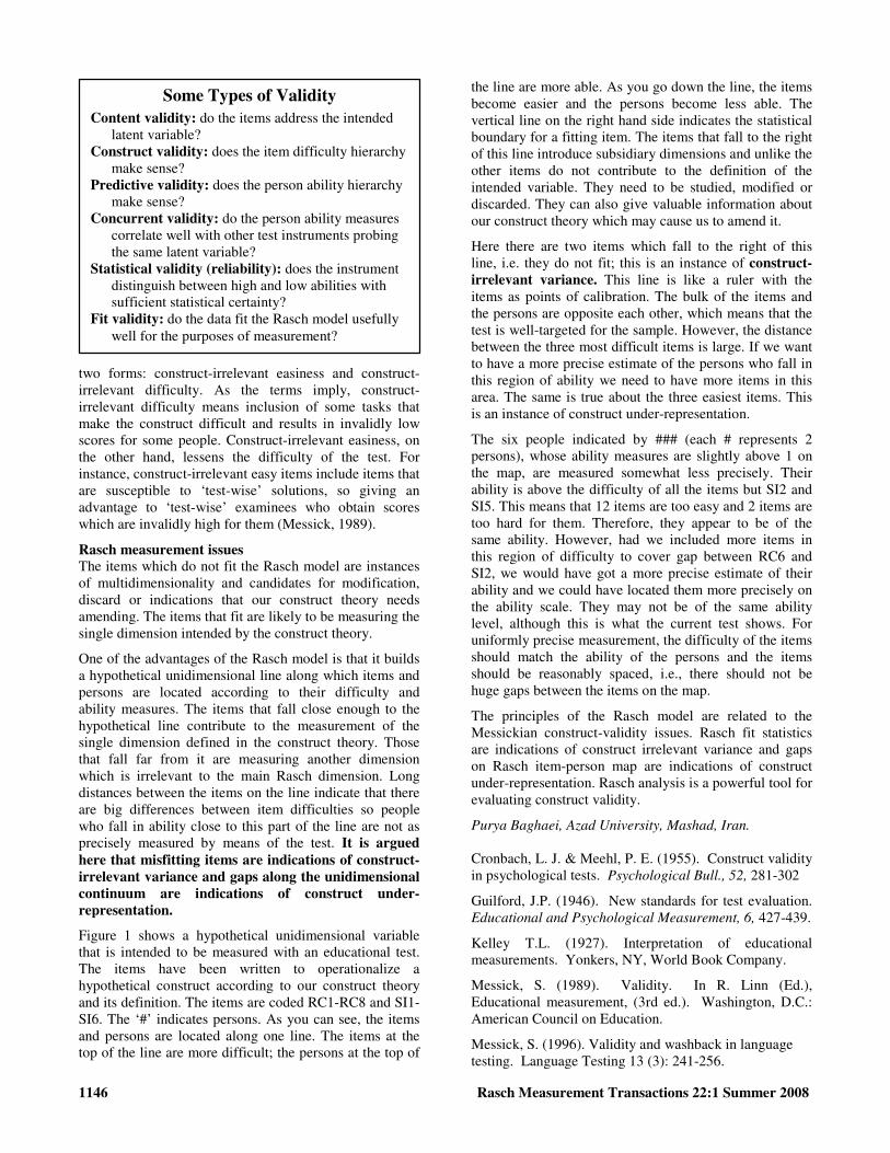
Figure 1 shows a hypothetical unidimensional variable that is intended to be measured with an educational test. The items have been written to operationalize a hypothetical construct according to our construct theory and its definition. The items are coded RC1-RC8 and SI1-SI6. The ‘#’ indicates persons. As you can see, the items and persons are located along one line. The items at the top of the line are more difficult; the persons at the top of

the line are more able. As you go down the line, the items become easier and the persons become less able. The vertical line on the right hand side indicates the statistical boundary for a fitting item. The items that fall to the right of this line introduce subsidiary dimensions and unlike the other items do not contribute to the definition of the intended variable. They need to be studied, modified or discarded. They can also give valuable information about our construct theory which may cause us to amend it.

Here there are two items which fall to the right of this line, i.e. they do not fit; this is an instance of construct-

irrelevant variance. This line is like a ruler with the items as points of calibration. The bulk of the items and the persons are opposite each other, which means that the test is well-targeted for the sample. However, the distance between the three most difficult items is large. If we want to have a more precise estimate of the persons who fall in this region of ability we need to have more items in this area. The same is true about the three easiest items. This is an instance of construct under-representation.

The six people indicated by ### (each # represents 2 persons), whose ability measures are slightly above 1 on the map, are measured somewhat less precisely. Their ability is above the difficulty of all the items but SI2 and SI5. This means that 12 items are too easy and 2 items are too hard for them. Therefore, they appear to be of the same ability. However, had we included more items in this region of difficulty to cover gap between RC6 and SI2, we would have got a more precise estimate of their ability and we could have located them more precisely on the ability scale. They may not be of the same ability level, although this is what the current test shows. For uniformly precise measurement, the difficulty of the items should match the ability of the persons and the items should be reasonably spaced, i.e., there should not be huge gaps between the items on the map.

The principles of the Rasch model are related to the Messickian construct-validity issues. Rasch fit statistics are indications of construct irrelevant variance and gaps on Rasch item-person map are indications of construct under-representation. Rasch analysis is a powerful tool for evaluating construct validity.

Purya Baghaei, Azad University, Mashad, Iran.

Cronbach, L. J. & Meehl, P. E. (1955). Construct validity in psychological tests. Psychological Bull., 52, 281-302

Guilford, J.P. (1946). New standards for test evaluation. Educational and Psychological Measurement, 6, 427-439.

Kelley T.L. (1927). Interpretation of educational measurements. Yonkers, NY, World Book Company.

Messick, S. (1989). Validity. In R. Linn (Ed.), Educational measurement, (3rd ed.). Washington, D.C.: American Council on Education.

Messick, S. (1996). Validity and washback in language testing. Language Testing 13 (3): 241-256.

Some Types of Validity

Content validity: do the items address the intended latent variable?

Construct validity: does the item difficulty hierarchy make sense?

Predictive validity: does the person ability hierarchy make sense?

Concurrent validity: do the person ability measures correlate well with other test instruments probing the same latent variable?

Statistical validity (reliability): does the instrument distinguish between high and low abilities with sufficient statistical certainty?

Fit validity: do the data fit the Rasch model usefully well for the purposes of measurement?


Notes on the 12th IMEKO TC1-TC7 Joint Symposium on Man, Science & Measurement

Held in Annecy, France, September 3-5, 2008

Two technical committees of the International Measurement Confederation, IMEKO, recently held their 12th symposium on philosophical and social issues associated with measurement and metrology, including psychosocial measurement applications, in Annecy, France. The committees involved were TC-1 (Education and Training in Measurement and Instrumentation) and TC-7 (Measurement Science). The meeting was conducted in English, with participants from 21 countries around the world. For this symposium, 77 papers were submitted, of which 60 were accepted. There were three plenary keynote lectures, and 74 registered attendees. A detailed program is available at http://imeko2008.scientific-symposium.com/fileadmin/progIMEKO2008V1.pdf .

In the first plenary session, Ludwik Finkelstein introduced himself as an elder preserving the organizational memory of the TC-7 on Measurement Science. Finkelstein touched on personal relationships from the past before describing new potentials for the technical committee beyond technical measurement issues. He was particularly interested in making the point that measurement theory

has been more thoroughly and rigorously grounded in

psychology, education and other fields than it has been

by metrological technologists. He contrasted strong versus weak measurement theories, and positivist versus anti-positivist philosophies of measurement, referring to the mathematical metaphysics of Galileo and Kelvin. Postmodernism was presented as anti-objective. The difference between metrological and psychometric reliability was pointed out, with an apparent assumption of inherent opposition and probable irreconcilability. Finkelstein also touched on issues of validity, public verifiability, standards, and traceability. He called for the introduction of traceability in psychosocial measurement.

William Fisher’s presentation on “New Metrological Horizons” began by referring to Finkelstein’s observations concerning the complementary potentials presented by probabilistic measurement theory’s articulation of invariance and parameter separation as criteria for objectivity, on the one hand, and by metrology’s focus on the traceability of individual measures to global reference standards. Evidence of the potential for traceability was offered in the form of the cross-sample invariance of item calibrations, the cross-instrument invariance of measures, and the cross-instrument/cross-sample invariance of constructs. Finkelstein responded to the presentation, saying that he was greatly encouraged and that his hopes for the future of measurement and metrology had been elevated.

In other presentations, subjective evaluations of sensory perceptions were compared with objective optical, haptic (tactual), and auditory measures. One presentation in this category was in effect a multifaceted judged visual

inspection. Another presentation involved a probabilistic model for dichotomous observations quite similar to a Rasch model. The majority of the papers concerned the design and optimization of practical measurement networks and systems. A natural place for Rasch measurement emerged in the context of evaluating the effectiveness of metrology education programs.

The second day’s plenary keynote was delivered by Paul De Bièvre, the Editor-In-Chief of the journal, Accreditation and Quality Assurance: Journal for

Quality, Comparability, and Reliability in Chemical

Measurement. His topic concerned the International Standards Organization’s (ISO) International Metrology Vocabulary. De Bièvre was enthused enough about Fisher’s presentation to invite an article introducing Rasch’s probabilistic models to the Accreditation and

Quality Assurance journal readership. Because of its similarity to De Bièvre’s own work in clarifying the vocabulary of metrology, Fisher offered his work on the ASTM E 2171 - 02 Standard Practice for Rating Scale

Measures for consideration.

TC-7 publishes Metrology & Measurement Systems, and prides itself on moving articles from submission to review to publication within three months. A recent special issue, “The Evolving Science of Measurement”, included articles with titles such as “Rankings as Ordinal Scale

Measurement Results” (outlining an elaborate two-dimensional analysis), “Advances and Generic Problems

in Instrument Design Methodology,” and “Self-

Configuring Measurement Networks.”

IMEKO membership is structured with member countries (39), friends of one or more technical committees, and honorary members.

TC-7 will participate in the XIX IMEKO World Congress that will be held in Lisbon, Portugal, September 6-11, 2009, with the theme of “Fundamental and Applied

Metrology.” Information on abstract submission is available on the site: http://www.imeko2009.it.pt/call.php through which abstracts can be submitted electronically. These are due December 15, 2008. Notification of acceptance will be made by April 15, 2009, and final paper submissions are due by June 1, 2009.

The next joint TC1-TC7 symposium on Man, Science &

Measurement will be held in London at City University, September 1-3, 2010, with the theme “Without

Measurement, There is No Science, and Without Science,

There is No Measurement.” Ludwik Finkelstein and Sanowar Khan will host the meeting. Professor Kahn indicated that there is interest in having a session on psychosocial measurement theory and practice.

William P. Fisher, Jr.

http://imeko2008.scientific

http://www.imeko2009.it.pt/call.php


ICOM International Conference on Outcomes Measurement Program Bethesda, Maryland - September 11-13, 2008

Thursday, September 11, 2008

Welcome and Opening Remarks: Thomas F. Hilton, Program Official at National Institute on Drug Abuse (NIDA), ICOM Host

Plenary Session 1 a. John Ware: ‘Advances in Health Measurement Models

and Data Collection Technologies: Implications for Standardizing Metrics & Making Assessment Tools More Practical.’

b. Michael Dennis: ‘Measurement Challenges in Substance Use and Dependency.’

c. A. Jackson Stenner: ‘Substantive Theory, General Objectivity and an Individual Centered Psychometrics.’

1A.1: IRT/Rasch in the Assessment of Change Chair: Rita Bode Discussant: Karon Cook a. Julie Carvalho: ‘Value Choices as Indicators of Healthy

Changes.’ b. Ken Conrad: ‘Measuring Change on the GAIN

Substance Problems Scale Using a Rasch Ruler.’ c. Donald Hedeker: ‘Application of Item Response

Theory Models for Intense Longitudinal Data on Smoking.’

1A.2: Theory and Importance of IRT/Rasch Chair: A. Jackson Stenner Discussant: David Andrich a. Robert Massof: ‘A Physical Metaphor for Explaining

the Mechanics of Rasch and IRT Models.’ b. Ann Doucette: ‘The Role of Measurement in

Evaluating the Effectiveness of Psychotherapy Outcomes.’

1A.3: Mental Health and Differential Item Functioning Chair: Benjamin Brodey Discussant: Paul Pilkonis a. Lohrasb Ahmadian, Robert Massof: ‘Validity of

Depression Measurement in Visually Impaired People - Investigating Differential Item Functioning by Chronic Diseases.’

b. Neusa Rocha, Marcelo Fleck, Mick Power, Donald Bushnell: ‘Cross-cultural evaluation of the WHOQOL-Bref domains in primary care depressed patients using Rasch Analysis.’

c. Heidi Crane, Laura E. Gibbons, Mari Kitahata, Paul K. Crane: ‘The PHQ-9 depression scale - Psychometric characteristics and differential item functioning (DIF) impact among HIV-infected individuals.’

1A.4: CAT Demonstration Barth Riley: ‘Application of computerized adaptive

testing in clinical substance abuse practice: Issues and strategies.’

1A.5: Demonstration LaVerne Hanes-Stevens: Teaching Clinicians How to

Relate Measurement Models to Clinical Practice: An example using the Global Appraisal of Individual Needs (GAIN).

Lunch a. Mark Wilson: ‘Latent Growth Item Response Models.’ b. Ronald Hambleton: ‘A Personal History of Computer-

Adaptive Testing - Short Version.’

1B.1: Health-related Quality of Life Chair: Alan Tennant Discussants: David Cella and John Ware a. David Feeny, Suzanne Mitchell, Bentson McFarland:

‘What are the key domains of health-related quality of life for methamphetamine users? Preliminary results using the Multi-Attribute System for Methamphetamine Use (MAS-MA) Questionnaire.’

b. Francisco Luis Pimentel, Jose Carlos Lopes: ‘HRQOL Instrument Construction Using Rasch Model.’

c. I-Chan Huang, Caprice A. Knapp, Dennis Revicki, Elizabeth A. Shenkman: ‘Differential item functioning in pediatric quality of life between children with and without special health care needs.’

1B.2: Measurement of Substance Use Disorders - I Chair: Brian Rush Discussant: A. Thomas McLellan a. Maria Orlando Edelen, Andrew Morral, Daniel

McCaffrey: ‘Creating an IRT-based adolescent substance use outcome measure.’

b. Betsy Feldman, Katherine E. Masyn: ‘Measuring and Modeling Adolescent Alcohol Use - A Simulation Study.’

1B.3: Demonstration David Andrich: ‘Interactive data analysis using the Rasch

Unidimensional Measurement Model - RUMM - Windows Software.’

1B.4: Demonstration Christine Fox, Svetlana Beltyukova: ‘Constructing Linear

Measures from Ordinal Data - An Example from Psychotherapy Research.’

1C.1: Assessing Physical Impairment and Differential Item Functioning

Chair: Barth Riley Discussant: Svetlana Beltyukova a. Gabrielle van der Velde, Dorcas E. Beaton, Sheilah

Hogg-Johnson, Eric Hurwitz, Alan Tennant: ‘Rasch Analysis of the Neck Disability Index.’

b. Sara Mottram, Elaine Thomas, George Peat: ‘Measuring locomotor disability in later life - do we need gender-specific scores?’

c. Kenneth Tang, Dorcas Beaton, Monique Gignac, Diane Lacaille, Elizabeth Badley, Aslam Anis, Claire Bombardier: ‘The Work Instability Scale for Rheumatoid Arthritis - Evaluation of Differential Item


Functioning in workers with Osteoarthritis and Rheumatoid Arthritis using Rasch Analysis.’

1C.2: Applications of the Global Appraisal of Individual Need (GAIN)

Chair: Michael Dennis Discussant: LaVerne Hanes-Stevens a. Sean Hosman, Sarah Kime: ‘Using the GAIN-SS in an

online format for screening, brief intervention and referral to treatment in King County.’

b. Richard Lennox, Michael Dennis, Mark Godley, Dave Sharar: ‘Behavioral Health Risk Assessment - Predicting Absenteeism and Workman’s Compensation Claims with the Gain Short Screener.’

1C.3: Item Functioning and Validation Issues Chair: Allen Heinemann Discussant: Bryce Reeve a. Benjamin Brodey, R.J. Wirth, D. Downing, J. Koble:

‘DIF analysis between publicly - and privately-funded persons receiving mental health treatment.’

b. Pey-Shan Wen, Craig A. Velozo, Shelley Heaton, Kay Waid-Ebbs, Neila Donovan: ‘Comparison of Patient, Caregiver and Health Professional Rating of a Functional Cognitive Measure.’

c. Mounir Mesbah: ‘A Empirical Curve to Check Unidimensionality and Local dependence of items.’

1C.4: Methodological Issues in Measurement Validation Chair: Tulshi Saha Discussant: Susan Embretson a. Richard Sawatzky, Jacek A. Kopec: ‘Examining

Sample Heterogeneity with Respect to the Measurement of Health Outcomes Relevant to Adults with Arthritis.’

b. Craig Velozo, Linda J. Young, Jia-Hwa Wang: ‘Developing Healthcare Measures - Monte Carlo Simulations to Determine Sample Size Requirements.’

c. Leigh Harrell, Edward W. Wolfe: ‘Effect of Correlation Between Dimensions on Model Recovery using AIC.’

1C.5: Questions and Answers for Those New to IRT/Rasch

Wine & Cheese Reception, and Poster Session a. Katherine Bevans, Christopher Forrest: ‘Polytomous

IRT analysis and item reduction of a child-reported wellbeing scale.’

b. Shu-Pi Chen. Bezruczko, N., Maher, J. M., Lawton, C. S., & Gulley, B. S.: ‘Functional Caregiving Item hierarchy Statistically Invariant across Preschoolers.’

c. Michael A. Kallen, DerShung Yang: ‘When increasing the number of quadrature points in parameter and score estimation no longer increases accuracy.’

d. Ian Kudel, Michael Edwards, Joel Tsevat: ‘Using the Nominal Model to Correct for Violations of Local Independence.’

e. Lisa M. Martin, Lori E. Stone, Linda L. Henry, Scott D. Barnett, Sharon L. Hunt, Eder L. Lemus, Niv Ad: ‘Resistance to Computerized Adaptive Testing (CAT) in Cardiac Surgery Patients.’

f. Michael T. McGill, Edward W. Wolfe: ‘Assessing Unidimensionality in Item Response Data via Principal Component Analysis of Residuals from the Rasch Model.’

g. Mesfin Mulatu: ‘Internal Mental Distress among Adolescents Entering Substance Abuse Treatment - Examining Measurement Equivalence across Racial/Ethnic and Gender Groups.’

Friday, September 12, 2008

Plenary Session 2 a. David Cella: ‘Patient-Reported Outcomes Measurement

Information System (PROMIS) Objectives and Progress Report.’

b. Expert Panel on PROMIS Methods and Results, including Karon Cook, Paul Pilkonis, and David Cella.

c. Robert Gibbons: ‘CAT Testing for Mood Disorder Screening.’

2A.1: Applications of Person Fit Statistics Chair/Discussant: A. Jackson Stenner a. Augustin Tristan, Claudia Ariza, María Mercedes

Durán: ‘Use of the Rasch model on cardiovascular post- surgery patients and nursing treatment.’

b. Ken Conrad: ‘Identifying Atypicals At Risk for Suicide Using Rasch Fit Statistics.’

c. Ya-Fen Chan, Barth Riley, Karen Conrad, Ken Conrad, Michael Dennis: ‘Crime, Violence and IRT/Rasch Measurement.’

2A.2: Applications of Computerized Adaptive Testing - I Chair/Discussant: Barth Riley a. Milena Anatchkova, Matthias Rose, Chris Dewey,

Catherine Sherbourne, John Williams: ‘A Mental Health Computerized Adaptive Test (MH-CAT) for Community Use.’

b. Ying Cheng: ‘When CAT meets CD - Computerized adaptive testing for cognitive diagnosis.’

c. Neila Donovan, Craig A. Velozo, Pey-Shan Wen, Shelley C. Heaton, Kay Waid-Ebbs: ‘Item Level Psychometric Properties of the Social Communication Construct Developed for a Computer Adaptive Measure of Functional Cognition for Traumatic Brain Injury.’

2A.3: Applications of IRT/Rasch in Mental Health Chair: Michael Fendrich Discussant: David Thissen a. Susan Faye Balaban, Aline Sayer, Sally I. Powers:

‘Refining the Measurement of Post Traumatic Stress Disorder Symptoms - An Application of Item Response Theory.’

b. Dennis Hart, Mark W. Werneke, Steven Z. George, James W. Matheson, Ying-Chih Wang, Karon F. Cook, Jerome E. Mioduski, Seung W. Choi: ‘Single items of fear-avoidance beliefs scales for work and physical activities accurately identified patients with high fear.’

c. Monica Erbacher, Karen M. Schmidt, Cindy Bergeman, Steven M. Boker: ‘Partial Credit Model Analysis of


the Positive and Negative Affect Schedule with Additional Items.’

2A.4: Assessing Education of Clinicians Chair: Craig Velozo Discussant: Mark Wilson a. Erick Guerrero: ‘Measuring Organizational Cultural

Competence in Substance Abuse Treatment.’ b. Ron Claus: ‘Using Rasch Modeling to Develop a

Measure of 12-Step Counseling Practices.’ c. Jean-Guy Blais, Carole Lambert, Bernard Charlin, Julie

Grondin, Robert Gagnon: ‘Scoring the Concordance of Script Test using a two-steps Rasch Partial Credit Modeling.’

d. Megan Dalton, Jenny Keating, Megan Davidson, Natalie de Morten: ‘Development of the Assessment of Physiotherapy Practice (APP) instrument - investigation of the psychometric properties using Rasch analysis.’

2A.5: CAT Demonstration a. Otto Walter: ‘Transitioning from fixed-questionnaires

to computer-adaptive tests: Balancing the items and the content.’

b. Matthias Rose: ‘Experiences with Computer Adaptive Tests within Clinical Practice.’

2A.6: Panel - Applying Unidimensional Models to Inherently Multidimensional Data

a. R. Darrell Bock: ‘Item Factor Analysis with the New POLYFACT Program.’

b. Robert Gibbons: ‘Bifactor IRT Models.’ c. Steven Reise: ‘The Bifactor Model as a Tool for

Solving Many Challenging Psychometric Issues.’

Lunch a. Alan Tennant: ‘Current issues in cross cultural

validity.’ b. A. Thomas McLellan: ‘Serving Clinical Measurement

Needs in Addiction - Translating the Science of Measurement into Clinical Value.’

2B.1: Applications of Computerized Adaptive Testing - II Chair: William Fisher Discussant: Otto Walter a. Karen Schmidt, Andrew J. Cook, David A. Roberts,

Karen C. Nelson, Brian R. Clark, B Eugene Parker, Jr., Susan E. Embretson: ‘Calibrating a Multidimensional CAT for Chronic Pain Assessment’.

b. Milena Anatchkova, Jason Fletcher, Mathias Rose, Chris Dewey, Hanne Melchior: ‘A Clinical Feasibility Test of Heart Failure Computerized Adaptive Test (HF-CAT).’

2B.2: Discerning Typologies with IRT/Rasch Chair: Kendon Conrad Discussant: Peter Delany a. Michael Dennis: ‘Variation in DSM-IV Symptom

Severity Depending on Type of Drug and Age: A Facets Analysis.’

b. Tulshi Saha, Bridget F. Grant: ‘Trajectories of Alcohol Use Disorder - An Application of a Repeated Measures, Hierarchical Rasch Model.’

c. James Henson, Brad T. Conner: ‘Substance Use and Different Types of Sensation Seekers - A Rasch Mixture Analysis.’

2B.3: Measurement of Treatment Processes Chair: Thomas Hilton Discussant: Paul Pilkonis a. Craig Henderson, Faye S. Taxman, Douglas W. Young:

‘A Rasch Model Analysis of Evidence-Based Treatment Practices Used in the Criminal Justice System.’

b. Panagiota Kitsantas, Faye Taxman: ‘Uncovering complex relationships of factors that impact offenders’ access to substance abuse programs - A regression tree analysis.’

c. Jason Chapman, Ashli J. Sheidow, Scott W. Henggeler: ‘Rasch-Based Development and Evaluation of a Test for Measuring Therapist Knowledge of Contingency Management for Adolescent Substance Use.’

2B.4: Measurement of Substance Use Disorders - II Chair: Michael Fendrich Discussant: Robert Massof a. Brian Rush, Saulo Castel: ‘Validation and comparison

of screening tools for mental disorders among people accessing substance abuse treatment.’

b. Allen Heinemann: ‘Using the Rasch Model to develop a substance abuse screening instrument for vocational rehabilitation agencies.’

2B.5: Demonstration Mark Wilson: ‘Constructing Measures: The BEAR

Assessment System.’

2C.1: Psychometric Issues in Measurement Validation Chair: Ya-Fen Chan Discussant: Craig Velozo a. Laura Stapleton, Tiffany A. Whittaker: ‘Obtaining item

response theory information from confirmatory factor analysis results.’

b. Jean-Guy Blais, Éric Dionne. ‘Skewed items responses distribution for the VF-14 visual functioning test - using Rasch models to explore collapsing of rating categories.’

c. Michelle Woodbury, Craig A. Velozo: ‘A Novel Application of Rasch Output - A Keyform Recovery Map to Guide Stroke Rehabilitation Goal-Setting and Treatment-Planning.’

d. Zhushan Li: ‘Rasch Related Loglinear Models with Ancillary Variables in Aggression Research.’

2C.2: Methodological Issues in Differential Item Functioning (DIF)

Chair/Discussant: Allen Heinemann a. Hao Song, Rebecca S. Lipner: ‘Exploring Practice

Setting Effects with Item Difficulty Variation on a Recertification Exam - Application of Two-Level Rasch Model.’


b. Barth Riley, Michael Dennis: ‘Distinguishing between Treatment Effects and the Influence of DIF in a Substance Abuse Outcome Measure Using Multiple Indicator Multiple Causes (MIMIC) Models.’

c. Rita Bode, Trudy Mallinson: ‘Consistency Across Samples in the Identification of DIF.’

2C.3: Perspectives on Current Practice and Beyond Chair: John Ware Discussant: David Andrich a. Stephen F. Butler, Ann Doucette: ‘Inflexxion’s

Computer Administered Addiction Severity Index - Successes, Challenges, and Future Directions.’

b. William Fisher: Uncertainty, the Welfare Economics of Medical Care, and New Metrological Horizons

2C.4: World Health Organization Measures Chair: Francisco Luis Pimentel Discussant: Alan Tennant a. T. Bedirhan Ustun: ‘World Health Organization

Disability Assessment Schedule II (WHODAS II) - Development, Psychometric Testing, and Applications.’

b. Neusa S. Rocha: ‘Measurement Properties of WHOQOL-Bref in Alcoholics Using Rasch Models.’

2C.5: Meet the Authors Chair: Barth Riley David Andrich, Susan Embretson, Christine Fox, Ronald

Hambleton, David Thissen and Mark Wilson.

Saturday, September 13, 2008

Plenary Session 3 a. David Andrich: ‘The polytomous Rasch model and

malfunctioning assessments in ordered categories - Implications for the responsible analysis of such assessments.’

b. Susan Embretson: ‘Item Response Theory Models for Complex Constructs.’

c. David Thissen: ‘The Future of Item Response Theory for Health Outcomes Measurement.’

Panel Session 3A The Future of Measurement in Behavioral Health Care Chair: Ken Conrad David Andrich, Michael Dennis, Thomas Hilton, A.

Thomas McLellan, Bryce Reeve, Alan Tennant and T. Bedirhan Ustun.Applying the Rasch Model

in the Human Sciences A hands-on introductory workshop

University of Johannesburg, South Africa

1, 2 and 3 December 2008

Conducted by Prof. Trevor Bond http://www.bondandfox.com/

The workshop will introduce participants to the conceptual underpinnings of the Rasch model and will support them to start analyzing their own data with Rasch analysis software. Participants will receive a copy of Trevor Bond’s co-authored book Applying the Rasch

Model: Fundamental Measurement in the Human

Sciences (LEA, 2007), which contains Bond&FoxSteps, the software used in the workshop. The structure of the workshop is:

Day 1: Introduction to the model. Analyzing tests with dichotomous items (including multiple choice items).

Day 2: Analyzing tests with polytomous items (such as Likert-type items)

Day 3: Evaluating the fit of data to the requirements of the model. Evaluating item and test functioning across demographic groups. Linking different forms of a test on a common scale. Publishing a Rasch measurement research paper.

The UJ Department of Human Resource Management and the People Assessment in Industry interest group invite you, your colleagues, and students to attend the workshop. A certificate of attendance will be issued to participants who attend all three days of the workshop. For more information please contact Deon de Bruin on 011 559 3944 or deondb /at/ uj.ac.za

Journal of Applied Measurement

Volume 9, Number 3. Fall 2008

Formalizing Dimension and Response Violations of Local Independence in the Unidimensional Rasch Model. Ida Marais and David Andrich, 200-215.

Calibration of Multiple-Choice Questionnaires to Assess Quantitative Indicators. Paola Annoni and Pieralda

Ferrari, 216-228.

The Impact of Data Collection Design, Linking Method, and Sample Size on Vertical Scaling Using the Rasch Model. Insu Paek, Michael J. Young, and Qing Yi,

229-248

Understanding the Unit in the Rasch Model. Stephen M.

Humphry and David Andrich, 249-264

Factor Structure of the Developmental Behavior Checklist using Confirmatory Factor Analysis of Polytomous Items. Daniel E. Bontempo, Scott. M. Hofer, Andrew

Mackinnon, Andrea M. Piccinin, Kylie Gray, Bruce

Tonge, and Stewart Einfeld, 265-280

Overcoming Vertical Equating Complications in the Calibration of an Integer Ability Scale for Measuring Outcomes of a Teaching Experiment. Andreas

Koukkoufis and Julian Williams, 281-304.

Understanding Rasch Measurement: Estimation of Decision Consistency Indices for Complex Assessments: Model Based Approaches. Matthew

Stearns and Richard M. Smith, 305-315

Richard M. Smith, Editor

JAM web site: www.jampress.org

http://www.bondandfox.com/

http://www.jampress.org


Formative and Reflective Models: Can a Rasch Analysis Tell the Difference?

Structural equation modeling (SEM) distinguishes two measurement models: reflective and formative (Edwards & Bagozzi, 2000). Figure 1 contrasts the very different causal structure hypothesized in the two models. In a reflective model (left panel), a latent variable (e.g., temperature, reading ability, or extraversion) is posited as the common cause of item or indicator behavior. The causal action flows from the latent variable to the indicators. Manipulation of the latent variable via changing pressure, instruction, or therapy causes a change in indicator behavior. Contrariwise, direct manipulation of a particular indicator is not expected to have a causal effect on the latent variable.

Reflective Formative

Figure 1. Causal Structures.

A formative model, illustrated on the right-hand side of Figure 1, posits a composite variable that summarizes the common variation in a collection of indicators. A composite variable is considered to be composed of independent, albeit correlated, variables. The causal action flows from the independent variables (indicators) to the composite variable. As noted by Bollen and Lennox (1991), these two models are conceptually, substantively, and psychometrically different. We suggest that the distinction between these models requires a careful consideration of the basis for inferring the direction of causal flow between the construct and its indicators.

Given the primacy of the causal story we tell about indicators and constructs, what kind of experiment, data, or analysis could differentiate between a latent variable story and a composite variable story? For example, does a Rasch analysis or a variable map or a set of fit statistics distinguish between these two different kinds of constructs? We think not! A Rasch model is an associational (think: correlational) model and as such is incapable of distinguishing between the latent-variable-causes-indicators story and the indicators-cause-composite-variable story.

Some examples from without and within the Rasch literature should help illustrate the distinction between formative and reflective models. The paradigmatic example of a formative or composite variable is

socioeconomic status (SES). Suppose the four indicators are education, occupational prestige, income, and neighborhood. Clearly, these indicators are the causes of SES rather than the reverse. If a person finishes four years of college, SES increases even if where the person lives, how much they earn, and their occupation stay the same. The causal flow is from indicators to construct because an increase in SES (job promotion) does not imply a simultaneous change in the other indicators. Bollen and Lennox (1991) gave another example: life stress. The four indicators are job loss, divorce, recent bodily injury, and death in the family. These indicators cause life stress. Change in life stress does not imply a uniform change in probabilities across the indicators. Lastly, the construct could be accuracy of eyewitness identification and its indicators could be recall of specific characteristics of the person of interest. These characteristics might include weight, hair style, eye color, clothing, facial hair, voice timber, and so on. Again, these indicators cause accuracy; they are not caused by changes in the probability of correct identification.

The examples of formative models presented above are drawn from the traditional test theory, factor analysis, and SEM literatures. Are Rasch analyses immune to confusion of formative and reflective models?

Imagine constructing a reading rating scale. A teacher might complete the rating scale at the beginning of the school year for each student in the class. Example items (rating structure) might include: (1) free or reduced price lunch (1,0), (2) periodicals in the home (0,1,2,3), (3) daily newspaper delivered at home, (4) student read a book for fun during the previous summer (1,0), (5) student placement in reading group (0,1,2,3), (6) student repeated a grade (1,0), (7) students current grade (1,2,3,…), (8) English is student’s first language (1,0), and so on. Now, suppose that each student, in addition to being rated by the teacher, took a Lexile-calibrated reading test. The rating scale items and reading test items could be jointly analyzed using WINSTEPS or RUMM2020. The analysis could be anchored so that all item calibrations for the reading rating items would be denominated in Lexiles. After calibration, the best-fitting rating scale items might be organized into a final scale and accompanied by a scoring guide that converts raw counts on the rating scale into Lexile reader measures. The reading scale is conceptually a composite formative model. The causal action flows from the indicators to the construct. Arbitrary removal of two or three of the rating items could have a disastrous effect on the predictive power of the set and, thus, on the very definition of the construct, whereas, removal of two or three reading items from a reading test will not alter the construct’s definition. Indicators (e.g., items) are exchangeable in the reflective case and definitional in the formative case.


Perline, Wainer, and Wright (1979), in a classic paper, used parole data to “measure a latent trait which might be labeled ‘the ability to successfully complete parole without any violations’” (p. 235). Nine dichotomously scored items rated for each of 490 participants were submitted to a BICAL analysis. The items were rated for presence or absence of: high school diploma or GED, 18 years or older at first incarceration, two or less prior convictions, no history of opiate or barbiturate use, release plan to live with spouse or children, and so on. The authors concluded, “In summary, the parole data appeared to fit [the Rasch Model] overall. . . . However, when the specific test for item stability over score groups was performed . . . there were serious signs of item

instability” (p. 249). For our purposes, we simply note that the Rasch analysis was interpreted as indicating a latent variable when it seems clear that it is likely a composite or formative construct.

A typical Rasch analysis carries no implication of manipulation and thus can make no claim about causal action. This means that there may be little information in a traditional Rasch analysis that speaks to whether the discovered regularity in the data is best characterized as reflective (latent variable) or formative (composite variable).

Rasch models are associational (i.e., correlational) models and because correlation is necessary but not sufficient for causation, a Rasch analysis cannot distinguish between composite and latent variable models. The Rubin-Holland framework for causal inference specifies: no causation

without manipulation. It seems that many Rasch calibration efforts omit the crucial last step in a latent variable argument: that is, answering the question, “What causes the variation that the measurement instrument detects?” (Borsboom, 2005). We suggest that there is no single piece of evidence more important to a construct’s definition than the causal relationship between the construct and its indicators.

A. Jackson Stenner, Donald S. Burdick, & Mark H. Stone

Bollen, K. A., & Lennox, R. (1991). Conventional wisdom on measurement: A structural equation perspective. Psychological Bulletin, 100, 305-314.

Borsboom, D. (2005). Measuring the Mind. Cambridge, MA: Cambridge University Press.

Burdick, D. S., Stone, M. H., & Stenner, A. J. (2006). The combined gas law and a Rasch reading law. Rasch

Measurement Transactions, 20(2), 1059-1060.

Edwards, J. R., & Bagozzi, R. P. (2000). On the nature and direction of relationships between constructs and measures. Psychological Methods, 5, 155-174.

Perline, R., Wainer H., & Wright, B. D. (1979). The Rasch model as additive conjoint measurement. Applied Psychological Measurement, 3(2), 237-255.

Perils of Ratings

Numeric ratings are one of the most abused components of any measurement and assessment system. They make people angry, destroy fragile working relationships, make one employee judge another, and create an artificial, thoroughly uncomfortable situation for both the rater and the person whose work is being rated.

The wonder to me, the way most numeric rating systems are designed, is why you would expect anything different from their use. If an organization takes unsubstantiated, undocumented, uncommunicated, secret numbers and springs a numeric rating on employees periodically, expect the worst.

Susan M. Heathfield, About.com

Rasch-related Coming Events

Sept. 11-13, 2008, Thurs.-Sat. International Conference on Outcomes Measurement (ICOM) , Washington D.C. http://icom-2008.org/

Sept. 17-19, 2008, Wed.-Fri. 1st International Conference on High School and College Educational Evaluation, Veracruz, Mexico http://www.ieia.mx.com

Sept. 2008 - Dec. 2009 3-day Rasch courses (A. Tennant, RUMM2020), Leeds, UK

http://www.leeds.ac.uk/medicine/rehabmed/psychometric

Oct. 14-15, 2008, Tues.-Wed. International Symposium on Measurement of Participation in Rehabilitation Research, Toronto, Canada

http://www.acrm.org/annual_conference/Precourses.cfm

Oct. 18-19, 2008, Sat.-Sun. An Introduction to Rasch Measurement: Theory and Applications (Smith & Smith, Winsteps, etc.), Chicago http://www.jampress.org/

Oct. 21-23, 2008, Tues.-Thurs. CAESL Center for the Assessment and Evaluation of Student Learning 2008, San Francisco CA http://www.caesl.org/

Oct. 31 - Nov. 28, 2008, Fri.-Fri. Many-Facet Rasch Measurement online course (M. Linacre, Facets), http://www.statistics.com/

Nov. 10, 2008, Monday III Workshop “Modelos de Rasch en Administración de Empresas”, Tenerife, Spain. http://www.iude.ull.es/

Dec. 1-3, 2008, Mon.-Wed. Workshop: Applying the Rasch Model in the Human Sciences (T. Bond, Bond&FoxSteps), deondb -at- uj.ac.za

Jan. 2-30, 2009, Fri.-Fri. Practical Rasch Measurement - Core Topics online course (M. Linacre, Winsteps), http://www.statistics.com/

April 13-17, 2009, Mon.-Fri. AERA Annual Meeting, San Diego, CA, USA, http://www.aera.net/

August, 2010 Probabilistic models for Measurement - 50 years, Conference, Copenhagen, Denmark

http://icom

http://www.ieia.mx.com

http://www.leeds.ac.uk/medicine/rehabmed/psychometric

http://www.acrm.org/annual_conference/Precourses.cfm

http://www.jampress.org/

http://www.caesl.org/

http://www.statistics.com/

http://www.iude.ull.es/

http://www.statistics.com/

http://www.aera.net/


The Expected Value of a Point-Biserial (or Similar) CorrelationInterpreting the observed value of a point-biserial correlation is made easier if we can compare the observed value with its expected value. Is the observed value much higher than the expected value (indicating dependency in the data) or much lower than expected (indicating unmodeled noise)? With knowledge of how the observed value compares with its expected value, there is no need for arbitrary rules such as “Delete items with point-biserials less than 0.2.”

The general formula for a Pearson correlation coefficient is:

Point-Biserial Correlation (including all observations

in the correlated raw score)

Suppose that Xn is Xni the observation of person n on item i. Yn is Rn, the raw score of person n, then the point-biserial correlation is:

where X i is the mean of the {Xni} for item i, and R is the mean of the Rn.

According to the Rasch model, the expected value of Xni is Eni and the model variance of Xni around its expectation is Wni. The model variances of X i, Rn, R are ignored here. Σ(Eni) = Σ(Xni), so that E i = X i.

Thus an estimate of the expected value of the point-measure correlation is given by the Rasch model proposition that: Xni = Eni ±√Wni

Since ±√Wni is a random residual, its cross-product with any other variable is modeled to be zero. Thus

which provides a convenient formula for computing the expected value of the point-biserial correlation.

Point-Biserial Correlation (excluding the current

observation in the correlated raw score)

where R' is the mean of the Rn-Xni.

is the expected value of the point-biserial correlation excluding the current observation.

Point-Measure Correlation

Similarly, suppose that Yn is Bn, the ability measure of person n, then the point-measure correlation is:

where B is the mean of the Bn.

Thus an estimate of the expected value of the point-measure correlation is:

which provides a convenient formula for computing the expected value of a point-measure correlation.

John Michael Linacre

Here is a worked example for a point-measure correlation:


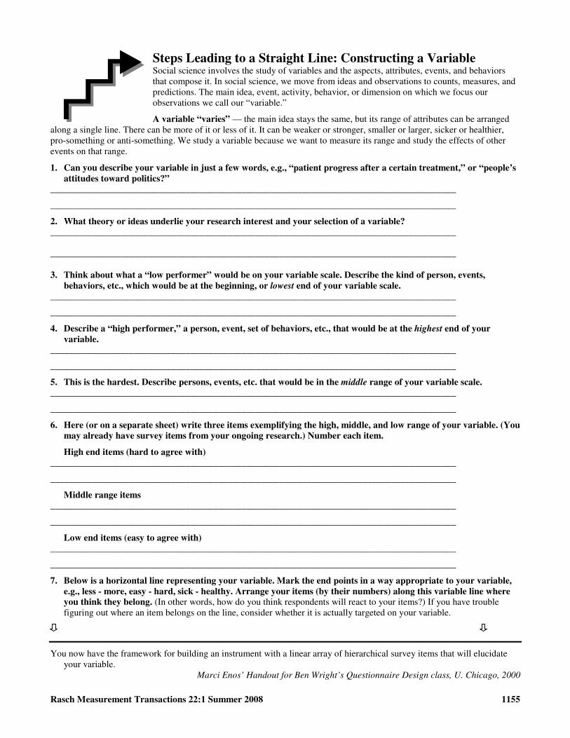
Steps Leading to a Straight Line: Constructing a Variable Social science involves the study of variables and the aspects, attributes, events, and behaviors that compose it. In social science, we move from ideas and observations to counts, measures, and predictions. The main idea, event, activity, behavior, or dimension on which we focus our observations we call our “variable.”

A variable “varies” — the main idea stays the same, but its range of attributes can be arranged along a single line. There can be more of it or less of it. It can be weaker or stronger, smaller or larger, sicker or healthier, pro-something or anti-something. We study a variable because we want to measure its range and study the effects of other events on that range.

1. Can you describe your variable in just a few words, e.g., “patient progress after a certain treatment,” or “people’s

attitudes toward politics?” _______________________________________________________________________________________

_______________________________________________________________________________________

2. What theory or ideas underlie your research interest and your selection of a variable?

_______________________________________________________________________________________

_______________________________________________________________________________________

3. Think about what a “low performer” would be on your variable scale. Describe the kind of person, events,

behaviors, etc., which would be at the beginning, or lowest end of your variable scale.

_______________________________________________________________________________________

_______________________________________________________________________________________

4. Describe a “high performer,” a person, event, set of behaviors, etc., that would be at the highest end of your

variable.

_______________________________________________________________________________________

_______________________________________________________________________________________

5. This is the hardest. Describe persons, events, etc. that would be in the middle range of your variable scale.

_______________________________________________________________________________________

_______________________________________________________________________________________

6. Here (or on a separate sheet) write three items exemplifying the high, middle, and low range of your variable. (You

may already have survey items from your ongoing research.) Number each item.

High end items (hard to agree with)

_______________________________________________________________________________________

_______________________________________________________________________________________

Middle range items _______________________________________________________________________________________

_______________________________________________________________________________________

Low end items (easy to agree with)

_______________________________________________________________________________________

_______________________________________________________________________________________

7. Below is a horizontal line representing your variable. Mark the end points in a way appropriate to your variable,

e.g., less - more, easy - hard, sick - healthy. Arrange your items (by their numbers) along this variable line where

you think they belong. (In other words, how do you think respondents will react to your items?) If you have trouble figuring out where an item belongs on the line, consider whether it is actually targeted on your variable.

You now have the framework for building an instrument with a linear array of hierarchical survey items that will elucidate your variable.

Marci Enos’ Handout for Ben Wright’s Questionnaire Design class, U. Chicago, 2000


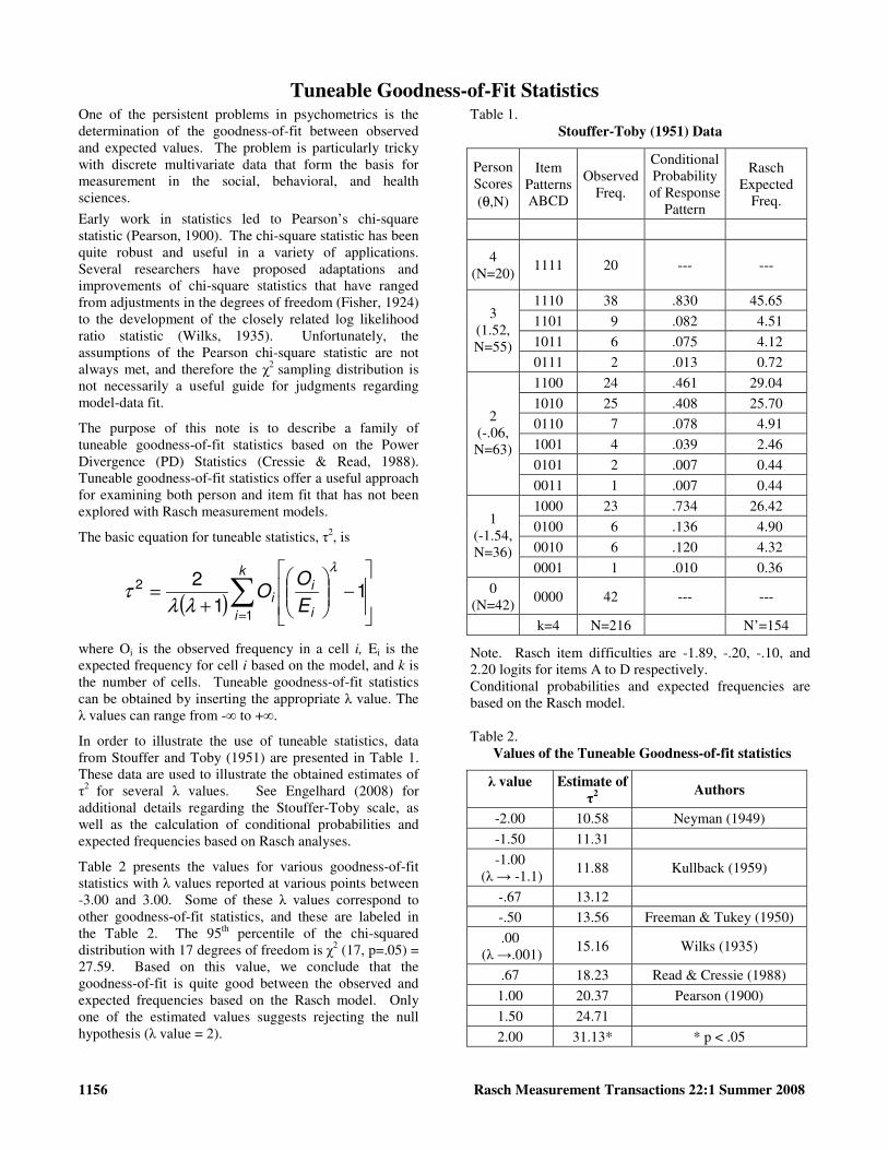
Tuneable Goodness-of-Fit StatisticsOne of the persistent problems in psychometrics is the determination of the goodness-of-fit between observed and expected values. The problem is particularly tricky with discrete multivariate data that form the basis for measurement in the social, behavioral, and health sciences.

Early work in statistics led to Pearson’s chi-square statistic (Pearson, 1900). The chi-square statistic has been quite robust and useful in a variety of applications. Several researchers have proposed adaptations and improvements of chi-square statistics that have ranged from adjustments in the degrees of freedom (Fisher, 1924) to the development of the closely related log likelihood ratio statistic (Wilks, 1935). Unfortunately, the assumptions of the Pearson chi-square statistic are not always met, and therefore the χ2 sampling distribution is not necessarily a useful guide for judgments regarding model-data fit.

The purpose of this note is to describe a family of tuneable goodness-of-fit statistics based on the Power Divergence (PD) Statistics (Cressie & Read, 1988). Tuneable goodness-of-fit statistics offer a useful approach for examining both person and item fit that has not been explored with Rasch measurement models.

The basic equation for tuneable statistics, τ2, is

( )∑=

−

+=

k

i i

ii

E

OO

1

21

1

2λ

λλτ

where Oi is the observed frequency in a cell i, Ei is the expected frequency for cell i based on the model, and k is the number of cells. Tuneable goodness-of-fit statistics can be obtained by inserting the appropriate λ value. The λ values can range from -∞ to +∞.

In order to illustrate the use of tuneable statistics, data from Stouffer and Toby (1951) are presented in Table 1. These data are used to illustrate the obtained estimates of τ2 for several λ values. See Engelhard (2008) for additional details regarding the Stouffer-Toby scale, as well as the calculation of conditional probabilities and expected frequencies based on Rasch analyses.

Table 2 presents the values for various goodness-of-fit statistics with λ values reported at various points between -3.00 and 3.00. Some of these λ values correspond to other goodness-of-fit statistics, and these are labeled in the Table 2. The 95th percentile of the chi-squared distribution with 17 degrees of freedom is χ2 (17, p=.05) = 27.59. Based on this value, we conclude that the goodness-of-fit is quite good between the observed and expected frequencies based on the Rasch model. Only one of the estimated values suggests rejecting the null hypothesis (λ value = 2).

Table 1. Stouffer-Toby (1951) Data

Person Scores (θ,N)

Item Patterns ABCD

Observed Freq.

Conditional Probability of Response

Pattern

Rasch Expected

Freq.

4 (N=20)

1111 20 --- ---

1110 38 .830 45.65

1101 9 .082 4.51

1011 6 .075 4.12

3 (1.52, N=55)

0111 2 .013 0.72

1100 24 .461 29.04

1010 25 .408 25.70

0110 7 .078 4.91

1001 4 .039 2.46

0101 2 .007 0.44

2 (-.06, N=63)

0011 1 .007 0.44

1000 23 .734 26.42

0100 6 .136 4.90

0010 6 .120 4.32

1 (-1.54, N=36)

0001 1 .010 0.36

0 (N=42)

0000 42 --- ---

k=4 N=216 N’=154

Note. Rasch item difficulties are -1.89, -.20, -.10, and 2.20 logits for items A to D respectively. Conditional probabilities and expected frequencies are based on the Rasch model. Table 2.

Values of the Tuneable Goodness-of-fit statistics

λ value

Estimate of

τ2

Authors

-2.00 10.58 Neyman (1949)

-1.50 11.31

-1.00 (λ → -1.1)

11.88 Kullback (1959)

-.67 13.12

-.50 13.56 Freeman & Tukey (1950)

.00 (λ →.001)

15.16 Wilks (1935)

.67 18.23 Read & Cressie (1988)

1.00 20.37 Pearson (1900)

1.50 24.71

2.00 31.13* * p < .05


This note describes a potentially useful set of tuneable goodness-of-fit statistics. It is important to recognize that explorations of goodness-of-fit should not involve a simple decision (e.g., reject the null hypothesis), but also require judgments and “cognitive evaluations of propositions” (Rozeboom, 1960, p. 427).

Additional research is needed on the utility of these tuneable statistics for making judgments regarding overall goodness-of-fit, item and person fit, and various approaches for defining and conducting residual analyses within the framework of Rasch measurement. This research should include research on the sampling distributions for various tuneable statistics applied to different aspects of goodness-of-fit, research on appropriate degrees of freedom, and research on the versions of the τ2 statistic that yield the most relevant substantive interpretations within the context of Rasch measurement theory and the construct being measured.

George Engelhard, Jr.

Emory University

Engelhard, G. (2008). Historical perspectives on invariant measurement: Guttman, Rasch, and Mokken. Measurement: Interdisciplinary Research and

Perspectives (6), 1-35.

Fisher, R.A. (1924). The conditions under which χ2 measures the discrepancy between observations and hypothesis. Journal of the Royal Statistical Society, 87, 442-450.

Freeman, D.H., & Tukey, J.W. (1950). Transformations related to the angular and the square root. Annals of

Mathematical Statistics, 21, 607-611.

Kullback, S. (1959). Information theory and statistics. New York: John Wiley.

Neyman, J. (1949). Contribution to the theory of the χ2

test. Proceedings of the First Berkeley Symposium on

Mathematical statistics and Probability, 239-273.

Pearson, K. (1900). On the criterion that a given system of deviations from the probable in the case of a correlated system of variables is such that it can be reasonably supposed to have arisen from random sampling. Philosophy Magazine, 50, 157-172.

Read, T.R.C., & Cressie, N.A.C. (1988). Goodness-of-fit

for discrete multivariate data. New York: Springer-Verlag.

Rozeboom, W.W. (1960). The fallacy of the null-hypothesis significance test. Psychological Bulletin, 57, 416-428.

Stouffer, S.A. & Toby, J. (1951). Role conflict and personality. The American Journal of Sociology, 56, 395-406.

Wilks, S.S. (1935). The likelihood test of independence in contingency tables. Annals of Mathematical Statistics,

6, 190-196.

Invariance and Item Stability

Kingsbury’s (2003) study of the long term stability of item parameter estimates in achievement testing has a number of important features.

First, rather than using parameter estimates from a set of items used in a single test, it investigated the stability of item parameter estimates in two large item banks used by the Northwest Evaluation Association (NWEA) to measure achievement in mathematics (> 2300 items) and reading (c.1400 items) with students from school years 2-10 in seven US states. Sample sizes for the 1999-2000 school year item calibrations ranged from 300 to 10,000 students.

Second, the elapsed time since initial calibration ranged from 7 to 22 years.

Third, and most importantly (for these purposes), “the one-parameter logistic (1PL) IRT model (Wright, 1977) was used to create and maintain the underlying measurement scales used with these banks.” While thousands of items have been added to these item banks over the course of time, each item has been connected to the original measurement scale through the use of IRT procedures and systematic Rasch measurement practices (Ingebo, 1997).

The observed correlations between the original and new item difficulties were extremely high (.967 in mathematics, .976 in reading), more like what would be expected if items were given to two samples at the same time, rather than samples separated by a time span from 7 to 20 years. Over that period, the average drift in the item difficulty parameters was .01 standard deviations of the mean item difficulty estimate. In Rasch measurement terms (i.e., focusing on impact on the measurement scales), the largest observed change in student scores moving from the original calibrations to the new calibrations was at the level of the minimal possible difference detectable by the tests, with over 99% of expected changes being less than the minimal detectable difference (Kingsbury, 2003).

NWEA have demonstrated measure-invariance beyond anything achieved anywhere else in the human sciences.

Trevor Bond

Hong Kong Institute of Education

Ingebo, G. S. (1997). Probability in the measure of achievement. Chicago, IL: MESA Press.

Kingsbury, G. (2003, April). A long-term study of the stability of item parameter estimates. Paper presented at the annual meeting of the American Educational Research Association, Chicago.

Wright, B.D. (1977). Solving Measurement Problems with the Rasch model. Journal of Educational Measurement, 14(2), 97-116.


The Cash Value of ReliabilityThe relationships among survey response rates, sample size, confidence intervals, reliability, and measurement error are often confused. Each of these are examined in turn, with an eye toward a systematic understanding of the role each plays in measurement. Reliability and precision estimates are of considerable utility, but their real cash value for practical applications is only rarely appreciated. This article aims to rectify confusions and provide practical guidance in the design and calibration of quality precision instruments.

Response Rates, Sample Size,

and Statistical Confidence

First, contrary to the concerns of many consumers of survey data, response rates often have little to do with the validity or reliability of survey data.

To see why, consider the following contrast of two extreme examples. Imagine that 1,000 survey responses are obtained from 1,000 persons selected as demographically representative of a population of 1 million, for a 100% response rate. Also imagine that 1,000 responses from exactly the same people are obtained, but this time in response to surveys that were mailed to a representative cross-section of 100,000 possible respondents, for a 1% response rate.

In either case, with both the 100% and the 1% response rates, the sample of 1,000 provides a confidence interval of, at worst, 3.1%, at 95% confidence for a dichotomous proportion, e.g., in an opinion poll, 52% ± 3.1% prefer one political candidate to another. As long as the relevant demographics of the respondents (sex, age, ethnicity, etc.) are in the same proportions as they are in the population, and there is no self-selection bias, then the 1% response rate is as valid as the 100% response rate. This insight underlies all sampling methodology.

The primary importance of response rates, then, concerns the cost of obtaining a given confidence interval and of avoiding selection bias. If 1,000 representative responses can be obtained from 1,000 mailed surveys, the cost of the 3.1% confidence interval in the response data is 1% of what the same confidence interval would cost when 1,000 representative responses are obtained from 100,000 mailed surveys.

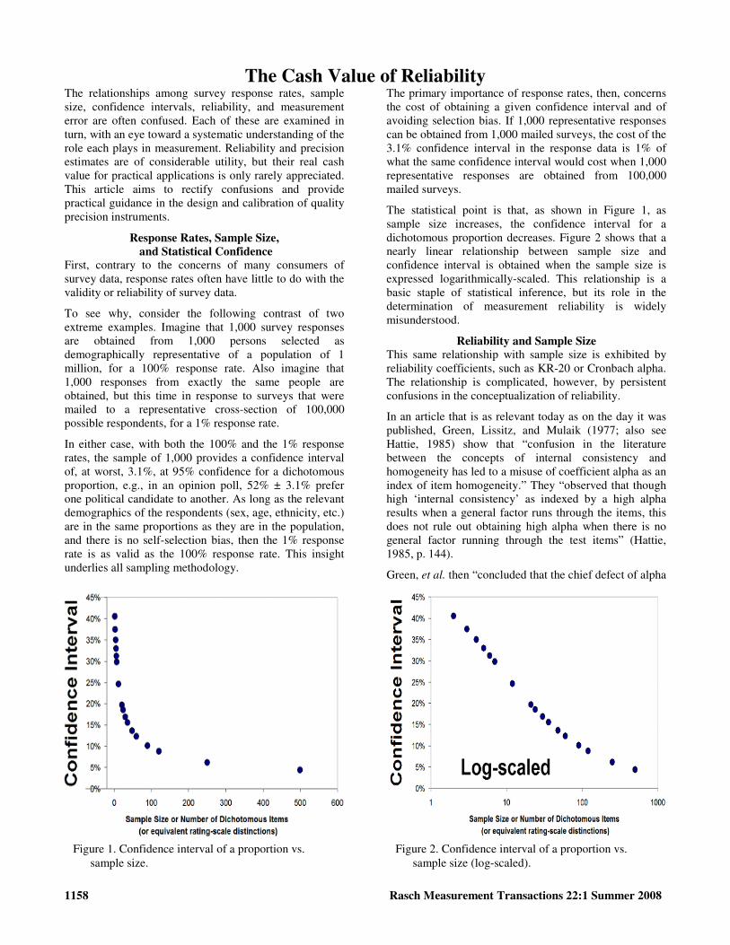
The statistical point is that, as shown in Figure 1, as sample size increases, the confidence interval for a dichotomous proportion decreases. Figure 2 shows that a nearly linear relationship between sample size and confidence interval is obtained when the sample size is expressed logarithmically-scaled. This relationship is a basic staple of statistical inference, but its role in the determination of measurement reliability is widely misunderstood.

Reliability and Sample Size

This same relationship with sample size is exhibited by reliability coefficients, such as KR-20 or Cronbach alpha. The relationship is complicated, however, by persistent confusions in the conceptualization of reliability.

In an article that is as relevant today as on the day it was published, Green, Lissitz, and Mulaik (1977; also see Hattie, 1985) show that “confusion in the literature between the concepts of internal consistency and homogeneity has led to a misuse of coefficient alpha as an index of item homogeneity.” They “observed that though high ‘internal consistency’ as indexed by a high alpha results when a general factor runs through the items, this does not rule out obtaining high alpha when there is no general factor running through the test items” (Hattie, 1985, p. 144).

Green, et al. then “concluded that the chief defect of alpha

Figure 1. Confidence interval of a proportion vs. sample size.

Figure 2. Confidence interval of a proportion vs. sample size (log-scaled).


as an index of dimensionality is its tendency to increase as the number of items increase” (Hattie, 1985, p. 144). Hattie (1985, p. 144) summarizes the state of affairs, saying that, “Unfortunately, there is no systematic relationship between the rank of a set of variables and how far alpha is below the true reliability. Alpha is not a monotonic function of unidimensionality.”

The desire for some indication of reliability, as expressed in terms of precision or repeatably reproducible measures, is, of course, perfectly reasonable. But interpreting alpha and other reliability coefficients as an index of data consistency or homogeneity is missing the point. To test data for the consistency needed for meaningful measurement based in sufficient statistics, one must first explicitly formulate and state the desired relationships in a mathematical model, and then check the data for the extent to which it actually embodies those relationships.

Model fit statistics (Smith, 2000) are typically employed for this purpose, not reliability coefficients.

However, what Hattie, and Green, et al., characterize as the “chief defect” of coefficient alpha, “its tendency to increase as the number of items increase,” has its productive place and positive purpose. This becomes apparent as one appreciates the extent to which the estimation of measurement and calibration errors in Rasch measurement is based in standard statistical sampling theory. The Spearman-Brown prophecy formula asserts a monotonic relationship between sample size and measurement reliability, expressed in the ratio of the error to the true standard deviation, as is illustrated in Linacre’s (1993) Rasch generalizability nomograph.

Reliability and Confidence Intervals

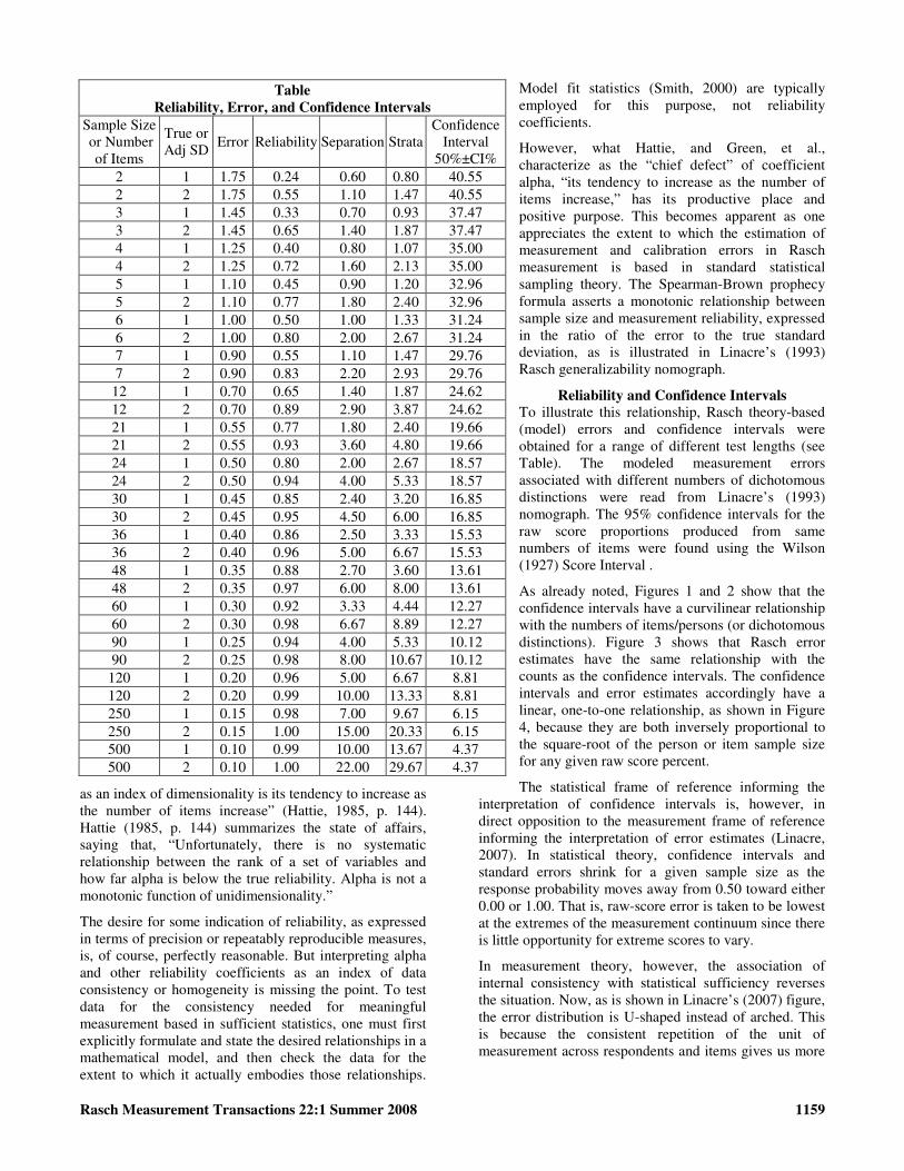
To illustrate this relationship, Rasch theory-based (model) errors and confidence intervals were obtained for a range of different test lengths (see Table). The modeled measurement errors associated with different numbers of dichotomous distinctions were read from Linacre’s (1993) nomograph. The 95% confidence intervals for the raw score proportions produced from same numbers of items were found using the Wilson (1927) Score Interval .

As already noted, Figures 1 and 2 show that the confidence intervals have a curvilinear relationship with the numbers of items/persons (or dichotomous distinctions). Figure 3 shows that Rasch error estimates have the same relationship with the counts as the confidence intervals. The confidence intervals and error estimates accordingly have a linear, one-to-one relationship, as shown in Figure 4, because they are both inversely proportional to the square-root of the person or item sample size for any given raw score percent.

The statistical frame of reference informing the interpretation of confidence intervals is, however, in direct opposition to the measurement frame of reference informing the interpretation of error estimates (Linacre, 2007). In statistical theory, confidence intervals and standard errors shrink for a given sample size as the response probability moves away from 0.50 toward either 0.00 or 1.00. That is, raw-score error is taken to be lowest at the extremes of the measurement continuum since there is little opportunity for extreme scores to vary.

In measurement theory, however, the association of internal consistency with statistical sufficiency reverses the situation. Now, as is shown in Linacre’s (2007) figure, the error distribution is U-shaped instead of arched. This is because the consistent repetition of the unit of measurement across respondents and items gives us more

Table

Reliability, Error, and Confidence Intervals

Sample Size or Number

of Items

True or Adj SD

Error Reliability Separation Strata Confidence

Interval 50%±CI%

2 1 1.75 0.24 0.60 0.80 40.55 2 2 1.75 0.55 1.10 1.47 40.55 3 1 1.45 0.33 0.70 0.93 37.47 3 2 1.45 0.65 1.40 1.87 37.47 4 1 1.25 0.40 0.80 1.07 35.00 4 2 1.25 0.72 1.60 2.13 35.00 5 1 1.10 0.45 0.90 1.20 32.96 5 2 1.10 0.77 1.80 2.40 32.96 6 1 1.00 0.50 1.00 1.33 31.24 6 2 1.00 0.80 2.00 2.67 31.24 7 1 0.90 0.55 1.10 1.47 29.76 7 2 0.90 0.83 2.20 2.93 29.76

12 1 0.70 0.65 1.40 1.87 24.62 12 2 0.70 0.89 2.90 3.87 24.62 21 1 0.55 0.77 1.80 2.40 19.66 21 2 0.55 0.93 3.60 4.80 19.66 24 1 0.50 0.80 2.00 2.67 18.57 24 2 0.50 0.94 4.00 5.33 18.57 30 1 0.45 0.85 2.40 3.20 16.85 30 2 0.45 0.95 4.50 6.00 16.85 36 1 0.40 0.86 2.50 3.33 15.53 36 2 0.40 0.96 5.00 6.67 15.53 48 1 0.35 0.88 2.70 3.60 13.61 48 2 0.35 0.97 6.00 8.00 13.61 60 1 0.30 0.92 3.33 4.44 12.27 60 2 0.30 0.98 6.67 8.89 12.27 90 1 0.25 0.94 4.00 5.33 10.12 90 2 0.25 0.98 8.00 10.67 10.12

120 1 0.20 0.96 5.00 6.67 8.81 120 2 0.20 0.99 10.00 13.33 8.81 250 1 0.15 0.98 7.00 9.67 6.15 250 2 0.15 1.00 15.00 20.33 6.15 500 1 0.10 0.99 10.00 13.67 4.37 500 2 0.10 1.00 22.00 29.67 4.37


confidence in the amounts indicated in the middle of the scale than they can at its extremes.

What this means is that the one-to-one correspondence of confidence intervals and error estimates shown in Figure 4 will hold only for any one response probability. As the probability of success or agreement, for instance, moves away from 0.50 (or as the difference between the measure and the calibration moves away from 0), the confidence interval will shrink while the Rasch measurement error will increase.

That said, plotting the errors and confidence intervals with Cronbach’s alpha reveals the effect of the true standard deviation in the measures or calibrations on the numbers of items associated with various errors or confidence intervals (Figures 5 and 6). Again, as the number of items increases, alpha for the person sample increases, and the confidence intervals and errors decrease, all else being equal. Similarly when the number of persons increases, an equivalent to alpha for the items increases.

The point of these exercises is to bring home the cash value of reliably reproducible precision in measurement. Hattie (1985, pp. 143-4) points out that,

“In his description of alpha Cronbach (1951) proved (1) that alpha is the mean of all possible split-half coefficients, (2) that alpha is the value expected when two random samples of items from a pool like those in the given test are correlated, and (3) that alpha is a lower bound to the proportion of test variance attributable to common factors among the items.”

This is why item estimates calibrated on separate samples correlate to about the mean of the scales’ reliabilities, and why person estimates measured using different samples of items correlate to about the mean of the measures’ reliabilities. (This statement is predicated on estimates of alpha that are based in the Rasch framework’s individualized error terms. Alpha assumes a single standard error derived from that proportion of the variance not attributable to a common factor. It accordingly is insensitive to off-target measures that will inflate Rasch error estimates to values often considerably higher than the modeled expectation. This means that alpha can over-estimate reliability, and that Rasch reliabilities will often be more conservative. This is especially the case in the presence of large proportions of missing data. For more information, see Linacre (1996).)

That is, the practical utility of reliability and Rasch separation statistics is that they indicate how many ranges there are in the measurement continuum that are repeatedly reproducible (Fisher, 1992). When reliability is lower than about 0.60, the top measure cannot be statistically distinguished from the bottom one with any confidence. Two instruments each measuring the same thing with a 0.60 reliability will produce measures that correlate about 0.60, less well than individual height and weight correlate.

Conversely, as reliability increases, so does the number of ranges in the scale that can be confidently distinguished. Measures from two instruments with reliabilities of

• 0.67 will tend to vary within two groups that can be separated with 95% confidence;

• 0.80 will vary within three groups;

• 0.90, four groups;

• 0.94, five groups;

• 0.96, six groups;

• 0.97, seven groups, and so on.

Figure 8 shows the theoretical relationship between strata (measurement or calibration ranges with centers three errors apart, Wright & Masters, 2002), Cronbach’s alpha, and sample size or the number of dichotomous distinctions. High reliability, combined with satisfactory model fit, makes it possible to realize the goal of creating measures that not only stay put while your back is turned, but that stay put even when you change instruments!

William P. Fisher, Jr., Ph.D.

Avatar International LLC

Fisher, W. P., Jr. (1992). Reliability statistics. Rasch Measurement Transactions, 6(3), 238 http://www.rasch.org/rmt/rmt63i.htm

Green, S. B., Lissitz, R. W., & Mulaik, S. A. (1977, Winter). Limitations of coefficient alpha as an index of test unidimensionality. Educational and Psychological Measurement, 37(4), 827-833.

Hattie, J. (1985, June). Methodology review: Assessing unidimensionality of tests and items. Applied Psychological Measurement, 9(2), 139-64.

Linacre, J. M. (1993). Rasch-based generalizability theory. Rasch Measurement Transactions, 7(1), 283-284; http://www.rasch.org/rmt/rmt71h.htm

Linacre, J. M. (1996). True-score reliability or Rasch statistical validity? Rasch Measurement Transactions, 9(4), 455 http://www.rasch.org/rmt/rmt94a.htm

Linacre, J. M. (2007). Standard errors and reliabilities: Rasch and raw score. Rasch Measurement Transactions, 20(4), 1086 http://www.rasch.org/rmt/rmt204f.htm

Smith, R. M. (2000). Fit analysis in latent trait measurement models. Journal of Applied Measurement, 1(2), 199-218.

Wilson, E. B. (1927). Probable inference, the law of succession, and statistical inference. Journal of the American Statistical Association 22: 209-212.

Wright B.D. & Masters G.N. (2002). Number of Person or Item Strata (4G+1)/3. Rasch Measurement Transactions, 2002, 16:3 p.888 http://www.rasch.org/rmt/rmt163f.htm

http://www.rasch.org/rmt/rmt63i.htm

http://www.rasch.org/rmt/rmt71h.htm

http://www.rasch.org/rmt/rmt94a.htm

http://www.rasch.org/rmt/rmt204f.htm

http://www.rasch.org/rmt/rmt163f.htm


Figure 3. Measurement error vs. sample size (log-scaled).

Figure 4. Measurement error vs. confidence interval of

proportion.

Figure 5. Reliability and confidence interval.

SD=1 on the left. SD=2 on the right.

Figure 6. Reliability and measurement error

Figure 7. Reliability and sample size.

Figure 8. Strata (measurements 3 errors apart).


Variance in Data Explained by Rasch MeasuresA Rasch model predicts that there will be a random aspect to the data. This is well understood. But what does sometimes surprise us is how large the random fraction is. The Figure shows the proportion of randomness predicted to exist in dichotomous data under various conditions.

The x-axis is the absolute difference between the mean of the person and item distributions, from 0 logits to 5 logits. The y-axis is the percent of variance in the data explained by the Rasch measures.

Each plotted line corresponds to one combination of standard deviations. The lesser of the person S.D. and the item S.D. is first, 0 to 5 logits, followed by “~”. Then the greater of the person S.D. and the item S.D.

Thus, the arrows indicate the line labeled “0-3”. This corresponds to a person S.D. of 0 logits and an item S.D. of 3 logits, or a person S.D. of 0 logits and an item S.D. of 3 logits. The Figure indicates that, with these measure distributions about 50% of the variance in the data is explained by the Rasch measures.

When the person and item S.D.s, are around 1 logit, then only 25% of the variance in the data is explained by the Rasch measures, but when the S.D.s are around 4 logits, then 75% of the variance is explained. Even with very wide person and item distributions with S.D.s of 5 logits only 80% of the variance in the data is explained.

Here are some percentages for empirical datasets:

% Variance

Explained Dataset

Winsteps

File name

71.1% Knox Cube Test exam1.txt

29.5% CAT test exam5.txt

0.0% coin tossing -

50.8% Liking for Science

(3 categories) example0.txt

37.5% NSF survey

(3 categories) interest.txt

30.0% NSF survey

(4 categories) agree.txt

78.7% FIM®

(7 categories) exam12.txt

Please email me your own percentages to add to this list.

John Michael Linacre

Editor, Rasch Measurement Transactions

The Rehabilitation Research and Training Center on

Measuring Outcomes and Effectiveness

at the Rehabilitation Institute of Chicago

International Symposium on

Measurement of Participation in

Rehabilitation Research

Tuesday-Wednesday, 14-15 October 2008

http://www.acrm.org/annual_conference/Preliminary_Program.cfm

Pre-Meeting Symposium to the 2008 ACRM-ASNR Joint Educational Conference in Toronto, Ontario, Canada at the Delta Chelsea Hotel, October 15-19, 2008.

This symposium will examine the construct of participation and its measurement, and nurture the development of an international consortium on the measurement of this important outcome by bringing together leaders in the field and establishing working groups on the key issues of participation measurement: conceptualization, operationalization, environmental influences, and personal characteristics.

Its objectives are to define and discuss the state-of-the-art in the measurement of participation, as well as its utility as an outcome measure for individuals with physical and cognitive disabilities who receive rehabilitation services.

Its faculty include: Allen Heinemann, PhD, ABPP (RP), FACRM, Tim Muzzio, PhD, Marcel Dijkers, PhD, FACRM, Marcel Post, PhD, Susan Magasi, PhD, Trudy Mallinson, PhD, OTR/L, NZROT, Margaret Brown, PhD, Jennifer Bogner, PhD, Rita Bode, PhD, Joy Hammel, PhD, OTR, Gale Whiteneck, PhD, FACRM, Alarcos Cieza, PhD, MPH, Susan Connors, Don Lollar, EdD, Mary Ann McColl, PhD, Alan Jette, PhD, David Tulsky, PhD, Luc Noreau, PhD, Carolyn Schwartz, ScD

http://www.acrm.org/annual_conference/Preliminary_Program.cfm

Documents

Rasch Measurement Transactions 22:1 - Institute for Objective