Embed Size (px)
Citation preview

RASPBERRY PI ASSEMBLER
Roger Ferrer IbanezCambridge, Cambridgeshire, U.K.
William J. PervinDallas, Texas, U.S.A.
September 11, 2017
i

Contents
1 Raspberry Pi Assembler 11.1 Writing Assembler . . . . . . . . . . . . . . . . . . . . . . . . . . . . . . 11.2 Our first program . . . . . . . . . . . . . . . . . . . . . . . . . . . . . . . 21.3 First program results . . . . . . . . . . . . . . . . . . . . . . . . . . . . . 3
2 ARM Registers 72.1 Basic arithmetic . . . . . . . . . . . . . . . . . . . . . . . . . . . . . . . . 7
3 Memory 93.1 Memory . . . . . . . . . . . . . . . . . . . . . . . . . . . . . . . . . . . . 93.2 Addresses . . . . . . . . . . . . . . . . . . . . . . . . . . . . . . . . . . . 93.3 Data . . . . . . . . . . . . . . . . . . . . . . . . . . . . . . . . . . . . . . 103.4 Sections . . . . . . . . . . . . . . . . . . . . . . . . . . . . . . . . . . . . 113.5 Load . . . . . . . . . . . . . . . . . . . . . . . . . . . . . . . . . . . . . . 113.6 Store . . . . . . . . . . . . . . . . . . . . . . . . . . . . . . . . . . . . . . 143.7 Programming style . . . . . . . . . . . . . . . . . . . . . . . . . . . . . . 15
4 Debugging 194.1 gdb . . . . . . . . . . . . . . . . . . . . . . . . . . . . . . . . . . . . . . . 19
5 Branching 255.1 A special register . . . . . . . . . . . . . . . . . . . . . . . . . . . . . . . 255.2 Unconditional branches . . . . . . . . . . . . . . . . . . . . . . . . . . . . 265.3 Conditional branches . . . . . . . . . . . . . . . . . . . . . . . . . . . . . 26
6 Control structures 316.1 If, then, else . . . . . . . . . . . . . . . . . . . . . . . . . . . . . . . . . . 316.2 Loops . . . . . . . . . . . . . . . . . . . . . . . . . . . . . . . . . . . . . 326.3 1 + 2 + 3 + 4 + · · · + 22 . . . . . . . . . . . . . . . . . . . . . . . . . . 326.4 3n + 1 . . . . . . . . . . . . . . . . . . . . . . . . . . . . . . . . . . . . . 35
7 Addressing modes 397.1 Indexing modes . . . . . . . . . . . . . . . . . . . . . . . . . . . . . . . . 397.2 Shifted operand . . . . . . . . . . . . . . . . . . . . . . . . . . . . . . . . 40
ii

Contents
8 Arrays and structures 438.1 Arrays and structures . . . . . . . . . . . . . . . . . . . . . . . . . . . . . 438.2 Defining arrays and structs . . . . . . . . . . . . . . . . . . . . . . . . . . 448.3 Naive approach without indexing modes . . . . . . . . . . . . . . . . . . 448.4 Indexing modes . . . . . . . . . . . . . . . . . . . . . . . . . . . . . . . . 45
8.4.1 Non-updating indexing modes . . . . . . . . . . . . . . . . . . . . 458.4.2 Updating indexing modes . . . . . . . . . . . . . . . . . . . . . . 468.4.3 Post-indexing modes . . . . . . . . . . . . . . . . . . . . . . . . . 478.4.4 Pre-indexing modes . . . . . . . . . . . . . . . . . . . . . . . . . . 48
8.5 Back to structures . . . . . . . . . . . . . . . . . . . . . . . . . . . . . . 498.6 Strings . . . . . . . . . . . . . . . . . . . . . . . . . . . . . . . . . . . . . 49
9 Functions 519.1 Do’s and don’ts of a function . . . . . . . . . . . . . . . . . . . . . . . . 51
9.1.1 New specially named registers . . . . . . . . . . . . . . . . . . . . 519.1.2 Passing parameters . . . . . . . . . . . . . . . . . . . . . . . . . . 529.1.3 Well behaved functions . . . . . . . . . . . . . . . . . . . . . . . . 529.1.4 Calling a function . . . . . . . . . . . . . . . . . . . . . . . . . . . 529.1.5 Leaving a function . . . . . . . . . . . . . . . . . . . . . . . . . . 529.1.6 Returning data from functions . . . . . . . . . . . . . . . . . . . . 53
9.2 Hello world . . . . . . . . . . . . . . . . . . . . . . . . . . . . . . . . . . 539.3 Real interaction! . . . . . . . . . . . . . . . . . . . . . . . . . . . . . . . 559.4 Our first function . . . . . . . . . . . . . . . . . . . . . . . . . . . . . . . 569.5 Unified Assembler Language . . . . . . . . . . . . . . . . . . . . . . . . . 59
10 Searching and Sorting 6110.1 Binary Search . . . . . . . . . . . . . . . . . . . . . . . . . . . . . . . . . 6110.2 Insertion Sort . . . . . . . . . . . . . . . . . . . . . . . . . . . . . . . . . 6410.3 Random Numbers . . . . . . . . . . . . . . . . . . . . . . . . . . . . . . . 6710.4 More Debugging . . . . . . . . . . . . . . . . . . . . . . . . . . . . . . . . 69
11 Recursion and the Stack 7111.1 Dynamic activation . . . . . . . . . . . . . . . . . . . . . . . . . . . . . . 7111.2 The stack . . . . . . . . . . . . . . . . . . . . . . . . . . . . . . . . . . . 7211.3 Factorial . . . . . . . . . . . . . . . . . . . . . . . . . . . . . . . . . . . . 7411.4 Load and Store Multiple . . . . . . . . . . . . . . . . . . . . . . . . . . . 7711.5 Factorial again . . . . . . . . . . . . . . . . . . . . . . . . . . . . . . . . 7811.6 Tail-recursion . . . . . . . . . . . . . . . . . . . . . . . . . . . . . . . . . 8011.7 Dynamic Programming . . . . . . . . . . . . . . . . . . . . . . . . . . . . 82
12 Conditional Execution 8712.1 Predication . . . . . . . . . . . . . . . . . . . . . . . . . . . . . . . . . . 8712.2 The pipe line of instructions . . . . . . . . . . . . . . . . . . . . . . . . . 8812.3 Predication in ARM . . . . . . . . . . . . . . . . . . . . . . . . . . . . . 90
iii

Contents
12.4 Collatz conjecture revisited . . . . . . . . . . . . . . . . . . . . . . . . . . 9012.5 Adding predication . . . . . . . . . . . . . . . . . . . . . . . . . . . . . . 9212.6 Does it make any difference in performance? . . . . . . . . . . . . . . . . 9212.7 The s suffix . . . . . . . . . . . . . . . . . . . . . . . . . . . . . . . . . . 93
13 Floating-point Numbers 9713.1 IEEE-754 Standard . . . . . . . . . . . . . . . . . . . . . . . . . . . . . . 9713.2 Examples . . . . . . . . . . . . . . . . . . . . . . . . . . . . . . . . . . . 9913.3 Extremes . . . . . . . . . . . . . . . . . . . . . . . . . . . . . . . . . . . 10013.4 Exceptions . . . . . . . . . . . . . . . . . . . . . . . . . . . . . . . . . . . 10113.5 Accuracy . . . . . . . . . . . . . . . . . . . . . . . . . . . . . . . . . . . . 10113.6 *Fixed-point Numbers . . . . . . . . . . . . . . . . . . . . . . . . . . . . 103
14 Real Computations 10514.1 VFPv2 Registers . . . . . . . . . . . . . . . . . . . . . . . . . . . . . . . 10514.2 Arithmetic operations . . . . . . . . . . . . . . . . . . . . . . . . . . . . 10614.3 Load and Store . . . . . . . . . . . . . . . . . . . . . . . . . . . . . . . . 10814.4 Movements between registers . . . . . . . . . . . . . . . . . . . . . . . . . 10914.5 Conversions . . . . . . . . . . . . . . . . . . . . . . . . . . . . . . . . . . 11014.6 Modifying the fpscr . . . . . . . . . . . . . . . . . . . . . . . . . . . . . . 11114.7 Function call convention and floating-point registers . . . . . . . . . . . . 11114.8 Printing Floating-point Numbers . . . . . . . . . . . . . . . . . . . . . . 112
15 Pointers 11315.1 Passing data to functions . . . . . . . . . . . . . . . . . . . . . . . . . . . 11315.2 What is a pointer? . . . . . . . . . . . . . . . . . . . . . . . . . . . . . . 11315.3 Passing large amounts of data . . . . . . . . . . . . . . . . . . . . . . . . 11615.4 Passing a big array by value . . . . . . . . . . . . . . . . . . . . . . . . . 11715.5 Passing a big array by reference . . . . . . . . . . . . . . . . . . . . . . . 12115.6 Modifying data through pointers . . . . . . . . . . . . . . . . . . . . . . 12315.7 Returning more than one piece of data . . . . . . . . . . . . . . . . . . . 126
16 System Calls 12716.1 File I/O . . . . . . . . . . . . . . . . . . . . . . . . . . . . . . . . . . . . 12816.2 lseek . . . . . . . . . . . . . . . . . . . . . . . . . . . . . . . . . . . . . . 131
17 Local data 13317.1 The frame pointer . . . . . . . . . . . . . . . . . . . . . . . . . . . . . . . 13317.2 Dynamic link of the activation record . . . . . . . . . . . . . . . . . . . . 13417.3 What about parameters passed in the stack? . . . . . . . . . . . . . . . . 13717.4 Indexing through the frame pointer . . . . . . . . . . . . . . . . . . . . . 137
18 Inline Assembler in C Code 14318.1 The asm Statement . . . . . . . . . . . . . . . . . . . . . . . . . . . . . . 14318.2 Simple Example . . . . . . . . . . . . . . . . . . . . . . . . . . . . . . . . 144
iv
Contents
19 Thumb 14719.1 The Thumb instruction set . . . . . . . . . . . . . . . . . . . . . . . . . . 14719.2 Support of Thumb in Raspbian . . . . . . . . . . . . . . . . . . . . . . . 14719.3 Instructions . . . . . . . . . . . . . . . . . . . . . . . . . . . . . . . . . . 14719.4 From ARM to Thumb . . . . . . . . . . . . . . . . . . . . . . . . . . . . 14819.5 Calling functions in Thumb . . . . . . . . . . . . . . . . . . . . . . . . . 14919.6 From Thumb to ARM . . . . . . . . . . . . . . . . . . . . . . . . . . . . 15119.7 To know more . . . . . . . . . . . . . . . . . . . . . . . . . . . . . . . . . 152
20 Additional Topics 15320.1 ARM Instruction Set . . . . . . . . . . . . . . . . . . . . . . . . . . . . . 15320.2 Interrupt Handling . . . . . . . . . . . . . . . . . . . . . . . . . . . . . . 15420.3 To know more . . . . . . . . . . . . . . . . . . . . . . . . . . . . . . . . . 155
A ASCII Standard Character Set 157
B Integers 159B.1 Unsigned Integers . . . . . . . . . . . . . . . . . . . . . . . . . . . . . . . 159B.2 Signed-Magnitude Integers . . . . . . . . . . . . . . . . . . . . . . . . . . 159B.3 One’s Complement . . . . . . . . . . . . . . . . . . . . . . . . . . . . . . 160B.4 Two’s Complement . . . . . . . . . . . . . . . . . . . . . . . . . . . . . . 161B.5 Arithmetic and Overflow . . . . . . . . . . . . . . . . . . . . . . . . . . . 162B.6 Bitwise Operations . . . . . . . . . . . . . . . . . . . . . . . . . . . . . . 163
C Matrix Multiplication (R.F.I.) 165C.1 Matrix multiply . . . . . . . . . . . . . . . . . . . . . . . . . . . . . . . . 165C.2 Accessing a matrix . . . . . . . . . . . . . . . . . . . . . . . . . . . . . . 167C.3 Naive matrix multiply of 4×4 single-precision . . . . . . . . . . . . . . . 168C.4 Vectorial approach . . . . . . . . . . . . . . . . . . . . . . . . . . . . . . 172C.5 Fill the registers . . . . . . . . . . . . . . . . . . . . . . . . . . . . . . . . 174C.6 Reorder the accesses . . . . . . . . . . . . . . . . . . . . . . . . . . . . . 177C.7 Comparing versions . . . . . . . . . . . . . . . . . . . . . . . . . . . . . . 182
D Subword Data 185D.1 Loading . . . . . . . . . . . . . . . . . . . . . . . . . . . . . . . . . . . . 185D.2 Storing . . . . . . . . . . . . . . . . . . . . . . . . . . . . . . . . . . . . . 188D.3 Alignment restrictions . . . . . . . . . . . . . . . . . . . . . . . . . . . . 188
E GPIO 193E.1 Onboard led . . . . . . . . . . . . . . . . . . . . . . . . . . . . . . . . . . 193E.2 wiringPi . . . . . . . . . . . . . . . . . . . . . . . . . . . . . . . . . . . . 195E.3 GPIO pins . . . . . . . . . . . . . . . . . . . . . . . . . . . . . . . . . . . 195E.4 Light an LED . . . . . . . . . . . . . . . . . . . . . . . . . . . . . . . . . 196
Index 197
v


Preface
This text is based on the first author’s tutorial:
http : //thinkingeek.com/arm− assembler − raspberry − pi/
and the second author’s MIPS assembler book:
A Programmer′s Guide to Assembler
(McGraw-Hill Custom Publishing).
This work is licenced under the Creative Commons Attribution-NonCommercial-Share-Alike 4.0 International Licence. To view a copy of that licence, visit
http : //creativecommons.org/licences/by − nc− sa/4.0/
or send a letter to Creative Commons, PO Box 1866, Mountain View, CA 94042, USA.
Note to reader: Be sure to look at all the Projects, even if you do not try them out.They may contain new information that is used in later chapters.
Caveat: There is a new Raspberry Pi 3 with a 64-bit architecture and other greatfeatures for the same price! In this work we will continue to give the Raspberry Pi2 information and, fortunately, the 3 seems to be backward compatible; that is, ourprograms run on it as well. In particular, the GNU assembler as works as described.Unfortunately, it does not support the additional registers or other improvements inthe architecture. This book will be completely rewritten as soon as better software isavailable.
Emulator: There is a very nice free emulator for the Raspberry Pi available throughthe web called QEMU. It’s easy to use and comes in handy when you do not have youractual Pi with you and want to try something out.
Disclaimer: Don’t use any of our code for commercial purposes and expect it to work.The authors, ARM Ltd., and the Raspberry Pi Foundation take no responsibility forphysical or mental damage caused by using this text.
vii


1 Raspberry Pi Assembler
You will see that our explanations do not aim at being very thorough when describingthe architecture. We will try to be pragmatic.
ARM is a 32-bit architecture that has a simple goal in mind: flexibility. While this isgreat for integrators (as they have a lot of freedom when designing their hardware), itis not so good for system developers who have to cope with the differences in the ARMhardware. So in this text we will assume that everything is done on a Raspberry
Pi 2 Model B running Raspbian (the one with at least 2 USB ports and 512 MB ofRAM).
Some parts will be ARM-generic but others will be Raspberry Pi specific. We will notmake a distinction. The ARM website (http://infocenter.arm.com/) has a lot ofdocumentation. Use it!
1.1 Writing Assembler
An assembler language is just a thin syntactic layer on top of its binary code. Un-fortunately, while somewhat similar in concept, they differ greatly between differentarchitectures. Learning one will certainly help in learning others, but it will still requirelots of work.
Binary code is what a computer can run. Each architecture requires different binarycode which is why the assembler languages also differ. The code we generate will not runon an Intel c© processor, for example. It is composed of instructions that are encodedin a binary representation (such encodings are documented in the ARM manuals). Youcould write binary coded instructions but that would be painstaking (besides some othertechnicalities related to Linux itself that we can happily ignore now).
So we will write assembler – ARM assembler. Since the computer cannot run assemblercode, we have to get binary code from it. We use a tool called, well, an assembler toassemble the assembler code into binary code that we can run.
The program to do this is called as and we will use it to assemble our programs. Inparticular it is the GNU Assembler, which is the program from the GNU project andsometimes it is also known as gas for this reason.
1

1. Raspberry Pi Assembler
To prepare an assembler language program for the assembler, just open an editor likevim, nano, or emacs in Raspbian. Our assembler language files (called source files)will have a suffix .s. That is the usual convention for the ARM (some architecturesmay use .asm or some other convention).
1.2 Our first program
We have to start with something, so we will start with a ridiculously simple programwhich does nothing but return an error code.
1 /* -- first.s */
2 /* This is a comment */
3 .global main /* entry point must be global */
4 .func main /* ’main’ is a function */
5
6 main: /* This is main */
7 mov r0, #2 /* Put a 2 into register r0 */
8 bx lr /* Return from main */
The numbers in the left column are just line numbers so that we can refer to them inthis text. They are not part of the program. Create a file called first.s and enter thecontents (without line numbers) exactly as shown above. Save it.
To assemble the file enter the following command (write exactly what comes after the$ prompt), ignoring the line numbers as usual.
1 $ as -g -mfpu=vfpv2 -o first.o first.s
This will create a file named first.o. Now link this file to get an executable file inbinary. (This actually uses the GNU C compiler!)
2 $ gcc -o first first.o
If everything goes as expected, you will get an executable binary file called first. Thisis your program. Run it.
3 $ ./first
[Note: The prefix ./ tells the system to look in the current directory for the executablefile.] It should seem to do nothing. Yes, it is a bit disappointing, but it actually doessomething. Get its error code this time.
4 $ ./first ; echo $?
5 2
2

1.3. First program results
Great! That error code of 2 is not by chance, it is due to that #2 in line 7 of theassembler source code.
Since running the assembler and the linker soon becomes boring, it is recommendedthat you use the following Makefile file or the Windows batch file instead.
1 # Makefile
2 all: first
3 first: first.o
4 gcc -o $@ $+
5 first.o : first.s
6 as -g -mfpu=vfpv2 -o $@ $<
7 clean:
8 rm -vf first *.o
1 #!/bin/bash
2 as -g -mfpu=vfpv2 -o $1.o $1.s
3 gcc -o $1 $1.o
4 rm $1.o
5 ./$1 ; echo $?
1.3 First program results
We cheated a bit just to make things a bit easier. We wrote a C main function inassembler which only does return 2; . This way our assembler program was easierto write since the C runtime system would handle initialization and termination of theprogram for us. We will use this approach almost all the time since the Raspberry Pisystem comes with a C compiler and we might as well use it.
Let’s review every line of our minimal assembler file.
1 /* -- first.s */
2 /* This is a comment */
These are comments. Comments are enclosed in /* and */. Use them to document yourassembler code as they are ignored. As usual, do not nest /* and */ inside /* becauseit does not work. Assembler code is very hard to read so helpful comments are quitenecessary.
3 .global main /* entry point and must be global */
This is a directive for the GNU Assembler. Directives tell the GNU Assembler to dosomething special other than emit binary code. They start with a period ( . ) followedby the name of the directive and possibly some arguments. In this case we are sayingthat main is a global name; i.e., recognizable outside our program. This is neededbecause the C linker will call main at runtime. If it is not global, it will not be callableand the linking phase will fail.
4 .func main /* ’main’ is a function */
3

1. Raspberry Pi Assembler
Here we have another GNU assembler directive and it states that main is a function.This is important because an assembler program usually contains instructions (i.e.,code) but may also contain data. We need to explicitly state that main actually refersto a function, because it is code.
6 main: /* This is main */
Every line in the GNU Assembler language that is not a directive will be of the form
label: instruction parameters comments
We can omit any part or all four fields (since blank lines are ignored). A line with onlylabel: applies that label to the next line (you can have more than one label referringto the same thing that way). The instruction part is the ARM assembler languageitself. Of course if there is no instruction there would be no parameters. In this casewe are just defining main since there is no instruction to be emitted by the assembler.
7 mov r0, #2 /* Put a 2 inside the register r0 */
Whitespace (spaces or tabs) is ignored at the beginning of the line, but the indentationsuggests visually that this instruction belongs to the main function. Since assemblercode is very hard to read, such regular indentation is strongly recommended. Line 7is the mov instruction which means move. We move the integer 2 into the register r0.In the next chapter we will see more about registers, do not worry now. The syntaxmay seem awkward because the destination is actually at the left. In ARM syntax itis almost always at the left (just as in an assignment statement like: r0 = 2;) so weare saying something like move to register r0 the immediate value 2. We will see whatimmediate value means in ARM in the next chapter but obviously the # mark is beingused to indicate an actual number.
In summary, this instruction puts the number 2 inside the register r0 (this effectivelyoverwrites whatever register r0 may have had at that point).
8 bx lr /* Return from main */
This instruction bx means Branch and eXchange. We do not really care at this pointabout the exchange part. Branching means that we will change the flow of the instruc-tion execution. An ARM processor runs instructions sequentially, one after the other.Thus after the mov above, this bx instruction will be run (this sequential execution is notspecific to ARM, but what happens in almost all architectures). A branch instructionis used to change this implicit sequential execution. In this case we branch to whateveraddress the lr register contains. We do not care now what lr contains. It is enough tounderstand that this instruction just leaves the main function, thus effectively endingour program.
And the error code? Well, the result of main is the error code of the program and whenleaving the function such result must be stored in the register r0, so the mov instructionperformed by our main is actually setting the error code to 2.
4

1.3. First program results
Projects
1. Experiment with returning other numbers than just 2.
2. How large a return code gives the correct answer?
3. How large an integer can you use in line 7 and have it accepted by the assembler?
4. Since comments explaining each line are often recommended, there is another formof comment. In as and the QEMU emulator, the symbol used is the “at” sign( @ ) to indicate that the rest of the line is a comment and is to be ignored bythe assembler. Test your assembler and see what character is used – and thenuse it! Real assembler programmers almost always only use the /* . . . */
construct for multi-line or special comments.
5. Although it will be very useful to go through the GNU C Compiler gcc whenwe start studying input and output, at this stage we may just use the linker orLoaDer (ld) that comes with the system.
In addition, to avoid the C compiler completely, we may use a complicated callon the operating system (Raspbian) to exit. The input to the assembler as wouldbe the following program.s:
1 /* -- program.s */
2 .global _start
3 _start:
4 mov r0, #2
5 mov r7, #1
6 svc 0 @ or SWI 0 -- both work
Note that we are not writing a main program for the C compiler. We will treatthis much later. The call on the assembler followed by the loader appears in thefollowing.
1 # Makefile
2 all: first
3 first: first.o
4 ld -o $@ $+
5 first.o : first.s
6 as -g -mfpu=vfpv2 -o $@ $<
7 clean:
8 rm -vf first *.o
1 #!/bin/bash
2 as -g -mfpu=vfpv2 -o $1.o $1.s
3 ld -o $1 $1.o
4 rm $1.o
5 ./$1 ; echo $?
Note: The -g parameter to as will be important when we study debugging inChapter 4. The -mfpu=vfpv2 parameter will be necessary starting in Chapter 14.
5

1. Raspberry Pi Assembler
6. In order to avoid putting the prefix ./ in front of all our programs, we maychange the path of our operating system with the command:
export PATH=$PATH:/home/pi/code,
assuming that we have put all our code in the subdirectory “code”. Try it, butremember that commands like this one can really mess up your system!
6

2 ARM Registers
At its core, the processor in a computer is nothing but a powerful calculator. Calcula-tions can only be carried out using values stored in very tiny memories called registers.The ARM processor in a Raspberry Pi 2 has, in addition to some specialized registersto be discussed later, 16 integer registers and 32 floating point registers. The processoruses these registers to perform integer computations and floating point computations,respectively. We will put floating registers aside for now and eventually we will get backto them in a future chapter. Let’s focus on the integer registers.
Those 16 integer registers in our ARM processor have names from r0 to r15. They canhold 32 bits each. Of course these 32 bits can encode whatever you want. That said, itis convenient to represent integers in two’s complement form (see Appendix B) as thereare instructions which perform computations assuming this encoding. So from now on,except as noted, we will assume our registers contain integer values encoded in two’scomplement form.
Not all the registers from r0 to r15 can be used in exactly the same way – some arereserved for special purposes – but we will not care about that for now. Just assumewhat we do is correct.
2.1 Basic arithmetic
Almost every processor can do some basic arithmetic computations using the integerregisters. The same is true for ARM processors. You can ADD two registers. Let’smodify our example from the previous chapter.
1 /* -- sum01.s */
2 .global main
3 .func main
4
5 main:
6 mov r1, #3 /* r1 <- 3 */
7 mov r2, #4 /* r2 <- 4 */
8 add r0, r1, r2 /* r0 <- r1 + r2 */
9 bx lr
7

2. ARM Registers
If we assemble, compile, and run this program, the error code returned is, as expected,7 – the sum of the 3 in register r1 and the 4 in register r2.
$ ./sum01 ; echo $?
7
We note immediately that the add instruction takes three registers as parameters. Wewill treat this and other instructions in more detail soon but it is clear that the firstparameter must be where the result of the addition is placed while the other two pa-rameters are the registers whose contents are to be added.
Nothing prevents us from using r0 in a more clever and efficient way.
1 /* -- sum02.s */
2 .global main
3 .func main
4
5 main:
6 mov r0, #3 /* r0 <- 3 */
7 mov r1, #4 /* r1 <- 4 */
8 add r0, r0, r1 /* r0 <- r0 + r1 */
9 bx lr
Which behaves as expected but uses only two registers instead of three which may bean important consideration later.
$ ./sum02 ; echo $?
7
Projects
1. Try adding other values than just 3 and 4.
2. Can you do subtraction by adding a negative number?
3. Is a negative return code possible?
4. The term “immediate” prefixed to “value” comes from the fact that small numbersmay, in some computers and assemblers, be placed within the machine instructionand thus save a reference to memory (as described later). The “pound” or “hash”sign (#) is used to indicate that the following actually a number. Test to seewhat happens if it is omitted.
5. Rewrite sum02.s so that it does not require the C compiler.
8

3 Memory
We saw in Chapters 1 and 2 that we can move values to registers (using the mov instruc-tion) and add two registers (using add instruction). If our processor were only able towork on registers it would be rather limited.
3.1 Memory
A computer has a memory where code (.text in the assembler) and data are stored sothere must be some way to access it from the processor. A bit of digression here: In386 and x86-64 architectures, instructions can access registers or memory, so we couldadd two numbers, one of which is in memory. You cannot do this in an ARM processorwhere all operands must be in registers. We can work around this problem (not reallya problem but a deliberate design decision that goes beyond the scope of this text –but see the Project) by loading data to a register from memory and storing data froma register to memory.
These two special operations, loading and storing, that are instructions on their ownare usually called load and store. There are several ways to load and store data from/tomemory but in this chapter we will focus on the simplest ones: LoaD to Register (ldr)from memory and STore from Register (str) to memory.
Loading data from memory is a bit complicated because we need to talk about addresses.
3.2 Addresses
To access data in memory we need to give it a name. Otherwise we could not refer towhat piece of data we want. Fortunately, a computer does have a name for every byteof memory. It is the address. An address is a number – in our Raspberry Pi 2 a 32-bitnumber – that identifies every byte (that is 8 bits) of the memory. (See Figure 3.1)
When loading or storing data from/to memory we need to compute an address. Thisaddress can be computed in many ways. Each of this ways is called an addressing mode.The ARM processor in a Raspberry Pi 2 has several of these addressing modes and it
9

3. Memory
will take a while to explain them all later, so here we will consider just one: addressingthrough a register.
It is not by chance that the processor has integer registers of 32 bits and the addressesof the memory are 32 bit numbers. That means that we can keep an address inside aregister. Once we have an address inside a register, we can use that register to find theaddress in memory in which to load or store some piece of data.
Figure 3.1
3.3 Data
When running a program, memory contains not only the code emitted by the assembler(called text), but also the data to be used by the program. We were deliberately loosewhen describing labels of the assembler. Now we can unveil their deep meaning: labelsin the assembler are just symbolic names for addresses in your program. These addressesmay refer either to data or code. So far we have used only one label (main) to designatethe address of our main function. A label only denotes an address, never its contents.Bear that in mind.
We said that an assembler is a thin layer on top of the binary code. Well, that thinlayer may now look to you a bit thicker since the assembler tool (as) is left responsiblefor assigning values to the addresses of the labels. This way we can use these labels andthe assembler will do some magic to make it work.
Thus, we can define some datum and attach a label to its address. It is up to us,as assembler programmers, to ensure that the storage referenced by the label has theappropiate size and value.
Let’s define a 4 byte variable and initialize it to 3. We will give it the label myvar1.
10

3.4. Sections
.balign 4
myvar1:
.word 3
There are two new assembler directives in the example above: .balign and .word.When the assembler as encounters a .balign directive with parameter 4, it ensures thatthe next address will start on a 4-byte boundary. That is, the address of the next datumemitted (either an instruction or data) will be a multiple of 4 bytes. This is importantbecause the ARM processor imposes some restrictions on the addresses of the data withwhich you may work. This directive does nothing if the address was already aligned to4. Otherwise the assembler will emit some padding bytes, which are not used at all bythe program, so the alignment requested is fulfilled. It is possible that we could omitthis directive if all the entities emitted by the assembler were 4 bytes wide (4 bytes is32 bits), but as soon as we want to use multiple sized data this directive will becomemandatory.
Now we define the address of myvar1. Thanks to the previous .balign directive, weknow its address will be aligned on a 4 byte boundary.
The .word directive states that the assembler should emit the value of the argument ofthe directive as a 4 byte integer. In this case it will emit 4 bytes containing the value3. Note that we rely on the fact that .word emits 4 bytes because that is defined to bethe size of a word in the ARM architecture.
3.4 Sections
Data resides in memory like code but, due to some practical technicalities that we donot care about very much now, it is usually kept together in what is called the datasection. The .data directive tells the assembler to emit the entities in the data section.The .text directive makes a similar thing happen for code (The .func directive madethat unnecessary in the preceding code.) So we will put data after a .data directiveand code after a .text directive.
3.5 Load
Now we shall retrieve our example from Chapter 2 and enhance it with some accessesto memory. We first define two 4 byte variables myvar1 and myvar2, initialized to 3and 4 respectively. We will load their values using ldr, and perform an addition. Theresulting error code should be 7, just as in Chapter 2.
1 /* -- load01.s */
2
3 /* -- Data section */
4 .data
11

3. Memory
5
6 /* Ensure variable is 4-byte aligned */
7 .balign 4
8 /* Define storage for myvar1 */
9 myvar1:
10 /* Contents of myvar1 is 4 bytes containing the value 3 */
11 .word 3
12
13 /* Ensure variable is 4-byte aligned */
14 .balign 4
15 /* Define storage for myvar2 */
16 myvar2:
17 /* Contents of myvar2 is 4 bytes containing the value 4 */
18 .word 4
19
20 /* -- Code section */
21 .text
22
23 /* Ensure code is 4 byte aligned */
24 .balign 4
25 .global main
26 main:
27 ldr r1, addr_of_myvar1 /* r1 <- &myvar1 */
28 ldr r1, [r1] /* r1 <- *r1 */
29 ldr r2, addr_of_myvar2 /* r2 <- &myvar2 */
30 ldr r2, [r2] /* r2 <- *r2 */
31 add r0, r1, r2 /* r0 <- r1 + r2 */
32 bx lr
33
34 /* Labels needed to access data */
35 addr_of_myvar1: .word myvar1
36 addr_of_myvar2: .word myvar2
We have a complication in the example above because of limitations of the assembler(see the Projects for a simple solution available in our assembler). As you can see thereare four ldr instructions. We will try to explain their meaning. First, though, we haveto discuss the following two labels.
34 /* Labels needed to access data */
35 addr_of_myvar1: .word myvar1
36 addr_of_myvar2: .word myvar2
These two labels are addresses of memory locations that contain the addresses of myvar1and myvar2. You may be wondering why we need them if we already have the addressesof our data in labels myvar1 and myvar2. A detailed explanation is a bit long, but
12

3.5. Load
what happens here is that myvar1 and myvar2 are in a different section – in the .data
section. That section exists so that the program can modify it. That is why variablesare kept there. On the other hand, code is not usually modified by the program (forefficiency and for security reasons). That is one reason to have two different sectionswith different properties attached to them. But, we cannot directly access a symbol inone section from another one. Thus, we need some locations in the .code section thatcontain the addresses of enties in the .data section. The assembler as helps us.
When the assembler emits the binary code, .word myvar1 will not actually be theaddress of myvar1 but instead it will be a relocation. A relocation is the way theassembler emits an address, the exact value of which is unknown but will known whenthe program is linked (i.e., when generating the final executable). It is like saying “Ihave no idea where this variable will actually be, let the linker patch this value for melater”. So this addr of myvar1 will be used instead. The address of addr of myvar1
is in the same .text section. That value will be patched by the linker during thelinking phase (when the final executable is created and it knows where all the entitiesof our program will definitely be laid out in memory). This is why the linker (invokedinternally by the C compiler gcc) is called ld . It stands for Link eDitor.
27 ldr r1, addr_of_myvar1 /* r1 <- &myvar1 */
28 ldr r1, [r1] /* r1 <- *r1 */
Again, there are two loads. The first one in line 27 actually loads the relocation valueof the address of myvar1. That is, there is some data in memory, the address of whichis addr of myvar1, with a size of 4 bytes containing the real address of myvar1. Afterthe first ldr, in r1 we have the real address of myvar1. But we do not want the addressat all, but the contents of the memory at that address, thus we do a second ldr.
Figure 3.2
13

3. Memory
The two loads obviously have different syntaxes. The first ldr uses the symbolic addressof addr of myvar1 label. The second ldr uses the value stored in the register as theaddressing mode. So, in the second case we are using the value inside r1 as the addressas indicated by the square brackets. In the first case, we do not actually know what theassembler uses as the addressing mode, so we will ignore it for now.
The program finally loads the two 32 bit values from myvar1 and myvar2, that hadinitial values 3 and 4, adds them, and sets the result of the addition as the error codeof the program in the r0 register just before leaving main.
$ ./load01 ; echo $?
7
3.6 Store
We now take the previous example but instead of setting the initial values of myvar1and myvar2 to 3 and 4 respectively, we will set both to 0. We will then reuse the existingcode but prepend some assembler code to store the 3 and 4 in the variables.
1 /* -- store01.s */
2
3 /* -- Data section */
4 .data
5
6 /* Ensure variable is 4-byte aligned */
7 .align 4
8 /* Define storage for myvar1 */
9 myvar1:
10 /* Contents of myvar1 is just ’0’ */
11 .word 0
12
13 /* Ensure variable is 4-byte aligned */
14 .align 4
15 /* Define storage for myvar2 */
16 myvar2:
17 /* Contents of myvar2 is just ’0’ */
18 .word 0
19
20 /* -- Code section */
21 .text
22
23 /* Ensure code section starts 4 byte aligned */
14

3.7. Programming style
24 .balign 4
25 .global main
26 main:
27 ldr r1, addr_of_myvar1 /* r1 <- &myvar1 */
28 mov r3, #3 /* r3 <- 3 */
29 str r3, [r1] /* *r1 <- r3 */
30 ldr r2, addr_of_myvar2 /* r2 <- &myvar2 */
31 mov r3, #4 /* r3 <- 4 */
32 str r3, [r2] /* *r2 <- r3 */
33
34 /* Same instructions as above */
35 ldr r1, addr_of_myvar1 /* r1 <- &myvar1 */
36 ldr r1, [r1] /* r1 <- *r1 */
37 ldr r2, addr_of_myvar2 /* r2 <- &myvar2 */
38 ldr r2, [r2] /* r2 <- *r2 */
39 add r0, r1, r2
40 bx lr
41
42 /* Labels needed to access data */
43 addr_of_myvar1: .word myvar1
44 addr_of_myvar2: .word myvar2
Note an important oddity in the str instructions in lines 29 and 32 of this code. Thedestination operand of the instruction is not the first operand. Instead the first operandis the source register and the second operand is the destination register.
$ ./store01; echo $?
7
3.7 Programming style
While the code emitted by the assembler will probably remain the same, the style withwhich one programs can have an effect. First of all, most programming is done inan environment in which many programmers work together and so have to read otherpeople’s code. Assembler is notoriously hard to read so many comments are appropriate.In order to encourage having a comment on almost every line of assembler code, theas assembler (and most others) makes available another form of comment. Everythingfollowing the “at” symbol ( @ ) is ignored by the assembler. This is the preferredmethod of making comments, leaving the /* . . . */ construct for multiline orspecial comments.
Another simplification is made available to the programmer by the as assembler. Justas compilers usually do more than just compile code, assemblers often do much morethan just translate mnemonics into code. For example, the need to obtain the address of
15

3. Memory
data in the .data section happens so often that a special symbol is used for that ratherthan the cumbersome method outlined above. If one refers to =myvar in, say, a load(ldr) operation, all that relocation and other duties are taken care of by the assemblerand there is no need for the extra labels as we used in lines 43 and 44.
There are other assumptions one can usually make about what the assembler does. Forexample, we would expect that both the .data and the .text sections are started on4-byte boundaries, at least. In addition, if we know that the datum for which space isbeing reserved takes exactly four bytes, we don’t have to bother telling the assemblerthe redundant directive .balign again and again.
Here is a version of the same program that we will use in the next chapter.
1 /* -- store02.s */
2 .data
3 myvar1: .word 0
4 myvar2: .word 0
5 .text
6 .global main
7 main:
8 ldr r1, =myvar1 @ r1 <- &myvar1
9 mov r3, #3 @ r3 <- 3
10 str r3, [r1] @ *r1 <- r3
11 ldr r2, =myvar2 @ r2 <- &myvar2
12 mov r3, #4 @ r3 <- 4
13 str r3, [r2] @ *r2 <- r3
14 ldr r1, =myvar1 @ r1 <- &myvar1
15 ldr r1, [r1] @ r1 <- *r1
16 ldr r2, =myvar2 @ r2 <- &myvar2
17 ldr r2, [r2] @ r2 <- *r2
18 add r0, r1, r2
19 bx lr
Even more simplification is possible. If we are careful, we might notice times in whichthe contents of a register are not changed between two commands and so reloading theregister is not necessary. We will not go that far yet (but see the Projects).
Note: If the company for which you work has standards, follow them carefully. Otheremployees (and your boss) will expect your code to meet those standards.
Note: Try to avoid using any “tricks” in your code. If you feel you must, at leastdocument them very explicitly. Even if you think no one else will ever see your code,you will forget what you did by tomorrow.
Note: Be careful about using any special knowledge you have about the hardware,operating system, or compiler (or assembler) on your system. When a new and im-
16

3.7. Programming style
proved version of the operating system is installed, any “undocumented” features maydisappear. The same is true about all software. If your company changes hardware -what will happen to your code?
Projects
1. Test to see if the .balign directive is really needed at the beginning of either the.data or the .text sections in store01.s.
2. Between lines 5 and 6 in store01.s, add the line
S: .asciz "string"
and see what happens. Is it different if "string" is replaced by "string!"? [Note:The directive .asciz actually means emit the string of characters in its parameterusing the ASCII encoding and terminating it with zero (null) character as used inthe C language.]
3. Look up the definition and history of the Reduced Instruction Set Computer(RISC). In addition, consider the design decision made by the inventors to limitaccess to memory to the load and store operations. Investigate the relative speedsof programs that highly access memory to those that do not.
4. Explain why the instructions in lines 35 and 37 of store01.s are not necessary(try it out). Can lines 14 and 16 be eliminated in store02.s?
17


4 Debugging
As we learn the foundations of ARM assembler language programming, our exampleswill become longer and longer. Since it is easy to make mistakes, it is worth learning howto use the GNU Debugger gdb to debug your assembler code. If you have developedC/C++ programs in Linux and have never used gdb, shame on you. If you know gdb
this small chapter will explain to you how to debug assembler directly.
4.1 gdb
We will use the example store02 from Chapter 3. Start gdb specifying the programyou are going to debug. We will show the results from one run on our system. Similarresponses will be had by your program using the Raspberry Pi or the QEMU emulatorbut some of the numbers may change slightly.
$ gdb --args ./store02
GNU gdb (GDB) 7.4.1-debian
Copyright (C) 2012 Free Software Foundation, Inc.
License GPLv3+: GNU GPL version 3 or later <http://gnu.org/licenses/gpl.html>
This is free software: you are free to change and redistribute it.
There is NO WARRANTY, to the extent permitted by law. Type "show copying"
and "show warranty" for details.
This GDB was configured as "arm-linux-gnueabihf".
For bug reporting instructions, please see:
<htp://www.gnu.org/software/gdb/bugs/> ...
Reading symbols from /home/RPiA/Chapter03/store02 ... done.
(gdb)
We are in the interactive mode of gdb. In this mode you communicate with gdb usingcommands. There is a builtin help command called help. Or you can check the GNUDebugger Documentation
http://sourceware.org/gdb/current/onlinedocs/gdb/.
The first command to learn is
(gdb) quit
19

4. Debugging
Ok, now start gdb again. The program is not running yet. In fact gdb will not be ableto tell you many things about it since it does not have any debugging information. Butthat is fine, we are debugging assembler, so we do not need much debugging information.As a first step let’s start the program.
(gdb) start
Temporary breakpoint 1 at 0x8394 : file store02.s, line 14.
Starting program: /home/RPiA/Chapter03/store02
Temporary breakpoint 1, main () at store02.s : 9
9 mov r3, #3 @ r3 <- 3
This tells us that, gdb ran our program up to and including the first instruction main
(note that some systems may not execute the first instruction). This is great becausewe have skipped all the initialization steps of the C library and have only run the firstinstruction of our main function. Let’s see what’s there. We will use the disassemble
command to translate the binary code back into assembler code.
(gdb) disassemble
Dump of assembler code for function main:
0x00008390 <+0>: ldr r1, [pc, #40] ; 0x83c0 <main+48>
=> 0x00008394 <+4>: mov r3, #3
0x00008398 <+8>: str r3, [r1]
0x0000839c <+12>: ldr r2, [pc, #32] ; 0x83c4 <main+52>
0x000083a0 <+16>: mov r3, #4
0x000083a4 <+20>: str r3, [r2]
0x000083a8 <+24>: ldr r1, [pc, #16] ; 0x83c0 <main+48>
0x000083ac <+28>: ldr r1, [r1]
0x000083b0 <+32>: ldr r2, [pc, #12] ; 0x83c4 <main+52>
0x000083b4 <+36>: ldr r2, [r2]
0x000083b8 <+40>: add r0, r1, r2
0x000083bc <+44>: bx lr
0x000083c0 <+48>: andeq r0,r1,r4,ror #10
0x000083C4 <+52>: andeq r0,r1,r8,ror #10
End of assembler dump.
This is very complicated but gives us a great deal of information. First, we see thatour program main has been placed in memory at location 0x00008390. Next, the firstinstruction in our code was ldr r1, =myvar1 but that has been linked to the actualaddress of myvar1 at 0x83c0 which is 48 bytes from where main begins. Down therewe see a strange instruction (andeq r0,r1,r4,ror #10) right after the last of our codeinstructions (bx lr). Had we continued with store01.s instead, we would rememberthat there were two more things in the .code section: places to keep the real addressesof myvar1 and myvar2. The assembler has actually done that for us but the debugger -that can’t know everything - has just translated those addresses into presumed assemblercode for some instructions.
20

4.1. gdb
Later we will also consider those addresses of the form [pc, #40] that are “pc-relative”addressing.
There is an arrow => pointing to the instruction we are going to run (it has not beenrun yet). Before running it, let’s inspect some registers. The commands should beself-explanatory (but the results may differ slightly on other systems).
(gdb) info registers r0 r1 r2 r3
r0 0x1 1
r1 0x10564 66916
r2 0xbefff86c 3204445692
r3 0x8390 33680
We see that the contents of the registers are given to us both in hex and decimal. Wecan modify registers using p which means print but also evaluates side effects. Forinstance, the following sets the value of register r0 to 2 and prints the result.
(gdb) p $r0 = 2
$1 = 2
gdb has printed $1, this is the counter it uses for the printed result and we can use itwhen needed, so we can skip some typing. The numbering system is not very usefulnow but it may be when we print a complicated expression.
Now we can again look at the registers (one could up-arrow twice).
(gdb) info registers r0 r1 r2 r3
r0 0x2 2
r1 0x10564 66916
r2 0xbefff86c 3204445692
r3 0x8390 33680
(gdb) p $1
$2 = 2
Now we could also use $2 to denote the second printed result, and so on. Now it is timeto run the second instruction and halt again.
(gdb) stepi
10 str r3, [r1] @ *r1 <- r3
In order to see what happened, let’s use disassemble, again.
(gdb) disassemble
Dump of assembler code for function main:
0x00008390 <+0>: ldr r1, [pc, #40] ; 0x83c0 <main+48>
0x00008394 <+4>: mov r3, #3
21

4. Debugging
=> 0x00008398 <+8>: str r3, [r1]
0x0000839c <+12>: ldr r2, [pc, #32] ; 0x83c4 <main+52>
0x000083a0 <+16>: mov r3, #4
0x000083a4 <+20>: str r3, [r2]
0x000083a8 <+24>: ldr r1, [pc, #16] ; 0x83c0 <main+48>
0x000083ac <+28>: ldr r1, [r1]
0x000083b0 <+32>: ldr r2, [pc, #12] ; 0x83c4 <main+52>
0x000083b4 <+36>: ldr r2, [r2]
0x000083b8 <+40>: add r0, r1, r2
0x000083bc <+44>: bx lr
0x000083c0 <+48>: andeq r0,r1,r4,ror #10
0x000083c4 <+52>: andeq r0,r1,r8,ror #10
End of assembler dump.
Again, let’s see what happened in the registers.
(gdb) info registers r0 r1 r2 r3
r0 0x2 2
r1 0x10564 66916
r2 0xbefff86c 3204445692
r3 0x3 3
That is exactly what we expected from the instruction mov r3, #3. Register r3 nowcontains the number 3. Now let’s perform the next instruction.
(gdb) stepi
11 ldr r2, =myvar2 @ r2 <- &myvar2
Let’s see what happened in register r1.
(gdb) info register r1
r1 0x10564 66919
Great, it has changed. In fact this is the address of myvar1. Let’s check that using itssymbolic name and C syntax.
(gdb) p &myvar1
$3 = (<data variable, no debug info> *) 0x10564
That again agrees with our expectations! In addition we can see what is in that variable:
(gdb) p myvar1
$4 = 3
Perfect. This was as expected since in this example we set zero as the initial value ofmyvar1 and then stored the number 3 there in this last instruction.
Now let us run until the end.
22

4.1. gdb
(gdb) continue
Continuing.
[Inferior 1 (process 2899) exited with code 07]
Which is, of course, the return code we wanted.
Projects
1. Step through more instructions of our program.
2. Download some manuals or quick reference cards from the web for future use.Look up other commands for gdb.
3. Look at memory locations in the .data section.
4. The ability to set breakpoints in gdb is very helpful. Note that when we give thedisassemble command we see on the left the addresses of the commands. In laterwork we will call on C functions for such things as reading and writing and wewill not want to stepi through the code for those functions when debugging ourcode. By setting breakpoints we can have the debugger stop right after performingthe action and see what’s in the registers or memory. Try setting and removingbreakpoints from your code.
23


5 Branching
Until now our small assembler programs execute one instruction after the other. If ourARM processor were only able to run this way it would be of limited use. It could notreact to existing conditions which may require different sequences of instructions. Thatis the purpose of the branch instructions.
5.1 A special register
In Chapter 2 we learned that our Raspberry Pi 2 ARM processor has 16 integer generalpurpose registers and we also said that some of them play special roles in our program.We deliberately ignored which registers were special as it was not relevant at that time.
But now it is relevant, at least for register r15. This register is very special, so special italso has another name: pc. It is unlikely that you see it termed r15 since it is confusing(although correct from the point of view of the ARM architecture). From now on wewill only use pc to name it.
pc stands for Program Counter. In general, the pc register (sometimes called theinstruction pointer in other architectures like the 386 or x86 64) contains the addressof the next instruction expected to be executed.
When the ARM processor executes an instruction, two things may happen during itsexecution. If the instruction does not modify the pc (and most instructions do not),the pc is just incremented by 4 (as if we did add pc, pc, #4). Why 4? Because inthe ARM architecture, instructions are 32 bits or 4 bytes wide, and so there are 4 bytesbetween every two instruction addresses. If the instruction modifies the pc then thenew value for the pc is used to address the next instruction instead.
Once the processor has fully executed an instruction, it uses the value in the pc asthe address for the next instruction to execute. This way, an instruction that does notmodify the pc will be followed by the next contiguous instruction in memory (since it hasbeen automatically increased by 4). This is called implicit sequencing of instructions:after one has run, usually the next one in memory runs. But if an instruction doesmodify the pc; for instance to a value other than pc + 4, then we can be running adifferent instruction of the program. This process of changing the value of pc is called
25

5. Branching
branching. In our processor this done using branch instructions.
5.2 Unconditional branches
You can tell the processor to branch unconditionally by using the instruction b (forBranch) and a label. Consider the following program.
/* -- branch01.s */
.text
.global main
main:
mov r0, #2 @ r0 <- 2
b end @ branch to ’end’
mov r0, #3 @ r0 <- 3
end:
bx lr
If you execute this program you will see that it returns an error code of 2.
$ ./branch01 ; echo $?
2
What happened is that instruction b end branched (modifying the pc register) to theinstruction at the label end, which is bx lr, the instruction we execute at the end ofour program. This way the instruction mov r0, #3 was not actually executed at all(the processor jumped over that instruction).
At this point the unconditional branch instruction b may look a bit useless but that isnot the case. In fact this instruction is essential in some contexts; in particular, whenlinked with conditional branching. But before we can talk about conditional branchingwe need to talk about conditions.
5.3 Conditional branches
If our processor were only able to branch when we put the unconditional branch b inour program, it would not be very useful. It is much more useful to branch when somecondition is met. So a processor should be able to evaluate some sort of conditions.
Before continuing, we need to unveil another register called the cpsr (for Current Pro-gram Status Register). This register is a bit special and directly modifying it is out ofthe scope of this chapter. That said, it keeps some values that can be read and updatedwhen executing an instruction. The contents of that register include four condition codebits, called flags, named N (Negative), Z (Zero), C (Carry) and V (oVerflow). These
26

5.3. Conditional branches
four condition code flags are usually read by branch instructions. Arithmetic instruc-tions and special testing and comparison instructions can update these condition codestoo if requested.
The semantics of these four condition codes in instructions updating the cpsr areroughly the following:
N Will be enabled (N == 1) if the result of the instruction yields a negative numberand will be disabled (N == 0) otherwise.
Z Will be enabled (Z == 1) if the result of the instruction yields a zero value and willbe disabled (Z == 0) if nonzero.
C Will be enabled if the result of the instruction is a value that requires a 33rd bit tobe fully represented. For instance an addition that overflows the 32 bit range ofintegers. There is a special case for C and subtractions where a non-borrowingsubtraction enables it, and it is disabled otherwise: subtracting a larger numberfrom a smaller one enables C, but it will be disabled if the subtraction is done inthe other order.
V Will be enabled if the result of the instruction yields a value that cannot be repre-sented in 32 bit two’s complement form and will be disabled otherwise.
So we have all the pieces needed to perform branches conditionally. But first, let’sstart comparing two values. We use the instruction cmp, standing for CoMPare, for thispurpose.
cmp r1, r2 /* updates the cpsr by doing "r1 - r2",
but r1 and r2 are not modified */
This instruction subtracts the value in the second register from the value in the firstregister setting the flags as appropriate. Consider the following examples of what couldhappen in the comparison instruction above?
• If r2 had a value (strictly) greater than r1 then N would be enabled because r1-r2would yield a negative result.
• If r1 and r2 had the same value, then Z would be enabled because r1-r2 would bezero.
• If r1 was 1 and r2 was 0 then r1-r2 would not borrow, so in this case C wouldbe enabled. If the values were swapped (r1 was 0 and r2 was 1) then C would bedisabled because the subtraction does borrow.
27
5. Branching
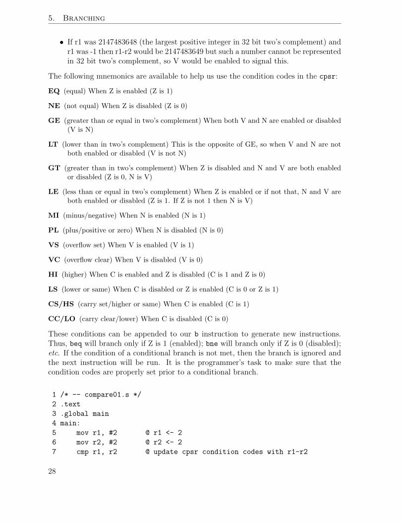
• If r1 was 2147483648 (the largest positive integer in 32 bit two’s complement) andr1 was -1 then r1-r2 would be 2147483649 but such a number cannot be representedin 32 bit two’s complement, so V would be enabled to signal this.
The following mnemonics are available to help us use the condition codes in the cpsr:
EQ (equal) When Z is enabled (Z is 1)
NE (not equal) When Z is disabled (Z is 0)
GE (greater than or equal in two’s complement) When both V and N are enabled or disabled(V is N)
LT (lower than in two’s complement) This is the opposite of GE, so when V and N are notboth enabled or disabled (V is not N)
GT (greater than in two’s complement) When Z is disabled and N and V are both enabledor disabled (Z is 0, N is V)
LE (less than or equal in two’s complement) When Z is enabled or if not that, N and V areboth enabled or disabled (Z is 1. If Z is not 1 then N is V)
MI (minus/negative) When N is enabled (N is 1)
PL (plus/positive or zero) When N is disabled (N is 0)
VS (overflow set) When V is enabled (V is 1)
VC (overflow clear) When V is disabled (V is 0)
HI (higher) When C is enabled and Z is disabled (C is 1 and Z is 0)
LS (lower or same) When C is disabled or Z is enabled (C is 0 or Z is 1)
CS/HS (carry set/higher or same) When C is enabled (C is 1)
CC/LO (carry clear/lower) When C is disabled (C is 0)
These conditions can be appended to our b instruction to generate new instructions.Thus, beq will branch only if Z is 1 (enabled); bne will branch only if Z is 0 (disabled);etc. If the condition of a conditional branch is not met, then the branch is ignored andthe next instruction will be run. It is the programmer’s task to make sure that thecondition codes are properly set prior to a conditional branch.
1 /* -- compare01.s */
2 .text
3 .global main
4 main:
5 mov r1, #2 @ r1 <- 2
6 mov r2, #2 @ r2 <- 2
7 cmp r1, r2 @ update cpsr condition codes with r1-r2
28

5.3. Conditional branches
8 beq case_equal @ branch to case_equal only if Z = 1
9 case_different:
10 mov r0, #2 @ r0 <- 2
11 b end @ branch to end
12 case_equal:
13 mov r0, #1 @ r0 <- 1
14 end:
15 bx lr
If you run this program it will return an error code of 1 because both r1 and r2 have thesame value. Now change mov r1, #2 in line 5 to be mov r1, #3 and the returned errorcode should be 2. Note that after case different we do not want to run the case equal
instructions, thus we have to branch to end (otherwise the error code would always be1).
Projects
1. Try out every one of the above mneumonics in the compare01 program withdifferent values for the immediate values!
2. Consider what you have to do if you want to change your code from using GE toLT.
3. There is a bal instruction which stands for Branch ALways. Compare it with b
and try to give a reason for its existence.
4. In addition to the cmp instruction, the ARM has other compare-like instructions.One example is cmn which is CoMpare Negative. Investigate the use of this andother test-like instructions.
29

6 Control structures
In the previous chapter we learned about branch instructions. They are really powerfultools because they allow us to express control structures. Structured programmingis an important milestone in better computing engineering so being able to map allthe usual structured programming constructs in assembler, in our processor, is a GoodThingTM.
6.1 If, then, else
This is one of the most basic control structures. In fact, we already used this structurein the previous chapter. Consider the following structure, where E is an expression andS1 and S2 are statements (they may be compound statements like { SA; SB; SC; })
if (E) then
S1
else
S2
A possible way to express this in ARM assembler could be the following
if_eval:
/* Assembler that evaluates E and updates the cpsr accordingly */
bXX else_part /* Here XX is the appropriate condition */
then_part:
/* assembler code for S1, the "then" part */
b end_of_if
else_part:
/* assembler code for S2, the "else" part */
end_of_if:
If there is no else part statement, we can replace bXX else part with bYY end of if
and omit the b end of if and the next two lines.
31

6. Control structures
6.2 Loops
This is another basic control structure in structured programming. While there areseveral types of loops, actually all can be reduced to the following structure.
while (E)
S
Supposedly S executes some instructions so than E eventually becomes false and theloop is left. Otherwise we would stay in the loop forever (sometimes this is what youwant but not in our examples). A way to implement these loops is as follows.
while_condition:
/* assembler code to evaluate E and update cpsr */
bXX end_of_loop /* If E is false, leave the loop right now */
/* assembler code for the statement S */
b while_condition /* Unconditional branch to the beginning */
end_of_loop:
A common loop involves iterating over a single range of integers, as in
for (i = L; i < N; i += K)
S
But this is nothing but
i = L;
while (i < N)
{
S;
i += K;
}
So we do not have to learn a new way to implement the loop itself.
6.3 1 + 2 + 3 + 4 + · · · + 22
As a first example let’s sum all the numbers from 1 to 22 (it will be explained shortlywhy we chose 22). The result of the sum is 253 (check it with a calculator). Of course itmakes little sense to compute something the result of which we know already, but thisis just an example.
01 /* -- loop01.s */
02 .text
03 .global main
32

6.3. 1 + 2 + 3 + 4 + · · · + 22
04 main:
05 mov r1, #0 @ r1 <- 0
06 mov r2, #1 @ r2 <- 1
07 loop:
08 cmp r2, #22 @ compare r2 and 22
09 bgt end @ branch if r2 > 22 to end
10 add r1, r1, r2 @ r1 <- r1 + r2
11 add r2, r2, #1 @ r2 <- r2 + 1
12 b loop
13 end:
14 mov r0, r1 @ r0 <- r1
15 bx lr
Here we are counting from 1 to 22. We will use register r2 as the counter. As you cansee in line 6 we initialize it to 1. The sum will be accumulated in register r1 and at theend of the program we move the contents of r1 into r0 to return the result of the sumas the error code of the program (we could have used r0 in all the code and avoidedthis final mov but we think it might be clearer this way).
In line 8 we compare r2 (remember, that is the counter that will go from 1 to 22) to22. This will update the cpsr so that we can check in line 9 if the comparison was suchthat r2 was greater than 22. If this is the case, we end the loop by branching to end.Otherwise we add the current value of r2 to the current value of r1 (remember, in r1
we accumulate the sum from 1 to 22).
Line 11 is an important one. We increase the value of r2, because we are counting from1 to 22 and we already added the current counter value in r2 to the result of the sumin r1. Then at line 12 we branch back at the beginning of the loop. Note that if line11 was not there we would hang as the comparison in line 8 would always be false andwe would never leave the loop in line 9!
$ ./loop01; echo $?
253
Now you could change the value in line 8 and try the program with, say, #100. Theresult should be 5050.
$ ./loop01; echo $?
186
What happened? Well, it happens that in Raspbian the error code of a program is anumber from 0 to 255 (8 bits). If the result is 5050, only the lower 8 bits of the numberare used. 5050 in binary is 1001110111010, its lower 8 bits are 10111010 which is exactly186. How can we check that the computed r1 is 5050 before ending the program? Let’suse gdb and display the first 9 instructions with disassemble.
33

6. Control structures
$ gdb loop01
...
(gdb) start
Temporary breakpoint 1 at 0x8390
Starting program: /home/RPiA/chapter07/loop01
Temporary breakpoint 1, 0x00008390 in main ()
(gdb) disas main,+(9*4)
Dump of assembler code from 0x8390 to 0x83b4:
0x00008390 <main+0>: mov r1, #0
0x00008394 <main+4>: mov r2, #1
0x00008398 <loop+0>: cmp r2, #100 ; 0x64
0x0000839c <loop+4>: bgt 0x83ac <end>
0x000083a0 <loop+8>: add r1, r1, r2
0x000083a4 <loop+12>: add r2, r2, #1
0x000083a8 <loop+16>: b 0x8398 <loop>
0x000083ac <end+0>: mov r0, r1
0x000083b0 <end+4>: bx lr
End of assembler dump.
Now that we know exactly where the instruction mov r0, r1 is, we may tell gdb to stopat 0x000083ac, right before executing that instruction. Here’s how to do it:
(gdb) break *0x000083ac
(gdb) cont
Continuing.
Breakpoint 2, 0x000083ac in end ()
(gdb) disas
Dump of assembler code for function end:
=> 0x000083ac <+0>: mov r0, r1
0x000083b0 <+4>: bx lr
End of assembler dump.
(gdb) info register r1
r1 0x13ba 5050
Great, this is what we expected. r1 actually contains 5050 but we could not see it dueto the limit in the size of the error code.
Maybe you have noticed that something odd happens with our labels being identifiedas functions. We will address this issue in a future chapter, but it is mostly harmlesshere.
34

6.4. 3n + 1
6.4 3n + 1
Let’s consider a bit more complicated example. This will be the famous 3n + 1 problem(also known as the Collatz conjecture). Given a number n we will divide it by 2 if itis even and multiply it by 3 and add one if it is odd.
if (n % 2 == 0)
n = n / 2;
else
n = 3*n + 1;
Before continuing, we should note that our ARM processor is able to multiply twonumbers together but we would have to learn about a somewhat complicated new in-struction (mul) which would detour us a bit. Instead we will use the following identity3n = 2n+n. We learned how to multiply or divide by two in Appendix B (using shifts).
The Collatz conjecture states that, for any number n, repeatedly applying this procedurewill eventually give us the number 1. Theoretically it could happen that this is not thecase: that there is a number for which the procedure never reaches 1. So far, no suchnumber has been found, but it has not been proven that one does not exist. If we wantto apply the previous procedure repeatedly, our program is to do something like this.
n = ...;
while (n != 1)
{
if (n % 2 == 0) n = n / 2;
else n = 3*n + 1;
}
If the Collatz conjecture were false, there would exist some n for which the code abovewould hang, never reaching 1. But as we said, no such number has been found.
1 /* -- collatz.s */
2 .text
3 .global main
4 main:
5 mov r1, #123 @ r1 <- 123 a trial number
6 mov r2, #0 @ r2 <- 0 the # of steps
7 loop:
8 cmp r1, #1 @ compare r1 and 1
9 beq end @ branch to end if r1 == 1
10
11 and r3, r1, #1 @ r3 <- r1 & 1 [mask]
12 cmp r3, #0 @ compare r3 and 0
13 bne odd @ branch to odd if r3 != 0
35

6. Control structures
14 even:
15 mov r1, r1, ASR #1 @ r1 <- (r1 >> 1) [divided by 2]
16 b end_loop
17 odd:
18 add r1, r1, r1, LSL #1 @ r1 <- r1 + (r1 << 1) [3n]
19 add r1, r1, #1 @ r1 <- r1 + 1 [3n+1]
20
21 end_loop:
22 add r2, r2, #1 @ r2 <- r2 + 1
23 b loop @ branch to loop
24
25 end:
26 mov r0, r2 @ number of steps
27 bx lr
In r1 we will keep the current value of the number n. In this case we will start withthe number 123. 123 reaches 1 in 46 steps: [123, 370, 185, 556, 278, 139, 418, 209, 628,314, 157, 472, 236, 118, 59, 178, 89, 268, 134, 67, 202, 101, 304, 152, 76, 38, 19, 58, 29,88, 44, 22, 11, 34, 17, 52, 26, 13, 40, 20, 10, 5, 16, 8, 4, 2, 1]. We will count the numberof steps in register r2. So we initialize r1 with 123 and r2 with 0 (no step has beenperformed yet).
At the beginning of the loop, in lines 8 and 9, we check if r1 is 1. We compare it to 1and if they are equal we leave the loop by branching to end.
Now that we know that r1 is not 1, we proceed to check if it is even or odd. To do thiswe use a new instruction which performs a bitwise and operation. An even number willhave its least significant bit (LSB) equal to 0, while an odd number will have the LSBequal to 1. So a bitwise and using the mask #1 will return 0 or 1 indicating even orodd numbers, respectively. In line 11 we keep the result of the bitwise and in registerr3 and then, in line 12, we compare it to 0. If it is not zero we branch to the label odd,otherwise we continue on to the even case.
Now some magic happens in line 15. This is a combined operation that ARM allows usto do. This is a mov but we do not move the value of r1 directly to r1 (which wouldbe doing nothing) but first we apply the operation Arithmetic Shift Right (ASR) to thevalue of r1 (to the value, not changing the register itself). Then this shifted value ismoved to the register r1. As described in Appendix B, an arithmetic shift right shiftsall the bits of a register to the right: the rightmost bit is effectively discarded and theleftmost is set to the same value as the leftmost bit prior the shift. Shifting a numberright one bit is the same as dividing that number by 2. So this mov r1, r1, ASR #1 isactually doing the integer operation r1 <- r1 / 2; .
Some similar magic happens for the even case in line 18. In this case we are doing anadd. The first and second operands must be registers (destination operand and the first
36

6.4. 3n + 1
source operand). The third operand (the second source operand) is combined with aLogical Shift Left (LSL). The value of the operand is shifted left 1 bit: the leftmost bitis discarded and the rightmost bit is set to 0. This is effectively multiplying the valueby 2. So we are adding r1 (which holds the value of n) to 2*r1. This is 3*r1, so 3 ∗ n.We keep this value in r1 again. In line 19 we add 1 to that value, so r1 ends up havingthe value 3n+ 1 that we wanted.
In the next chapter we will treat the shift operators LSL and ASR in more detail.
Finally, at the end of the loop, in line 22 we update r2 (remember it keeps the counterof our steps) and then we branch back to the beginning of the loop. Before ending theprogram we move the counter to r0 so we return the number of steps we used to reach1.
$ ./collatz; echo $?
46
Projects
1. Look up the original definition of the IF statement in FORTRAN. Since it had noelse clause, show how the unconditional branch ( b ) was necessary. Comment onhow that translates into the goto statement whose existance was highly criticisedin software engineering circles. Note that Java, while it does not have a goto
statement, reserves the word so that it cannot be used as an identifier but is keptjust in case there is such a statement added to the language someday.
2. Rewrite the if eval: code in our first example so that the else clause precedesthe if clause.
3. Note that both the while and the for statements test the condition before per-forming the loop body. Compare that to the until statement that always triesto perform the loop body at least once. Note that the original construct in FOR-TRAN always performed the body at least once, even if the condition failed.Rewrite a general until statement using a while statement instead.
4. Try out the Collatz conjecture with some larger numbers. Do you think you canstart with any number?
5. Can you think of any reason not to use r0 to hold the count in code collatz.s?If not, rewrite the code and test it.
Postscript
Kevin Millikin rightly pointed that usually a loop is not implemented in the way shownabove. He recommends a better way to do the loop of loop01.s as follows.
37

6. Control structures
1 /* -- loop02.s */
2 .text
3 .global main
4 main:
5 mov r1, #0 @ r1 <- 0
6 mov r2, #1 @ r2 <- 1
7 b check_loop @ unconditionally jump to end of loop
8 loop:
9 add r1, r1, r2 @ r1 <- r1 + r2
10 add r2, r2, #1 @ r2 <- r2 + 1
11 check_loop:
12 cmp r2, #22 @ compare r2 and 22
13 ble loop @ if r2 <= 22 goto beginning of loop
14 end:
15 mov r0, r1 @ r0 <- r1
16 bx lr
If you count the number of instruction in the two codes, there are 9 instructions inboth. But if you look carefully at Kevin’s proposal you will see that by unconditionallybranching to the end of the loop, and reversing the condition check, we can skip onebranch thus reducing the number of instructions of the loop itself from 5 to 4. One ofthe recommendations for good programming practices in any language has always beento have as few instructions within a loop as possible.
There is another advantage of this second version, though: there is only one branch inthe loop itself as we resort to implicit sequencing to reach again the two instructionsperforming the check. For reasons beyond the scope of this chapter, the execution of abranch instruction may negatively affect the performance of our programs. Processorshave mechanisms to mitigate the performance loss due to branches (and in fact theprocessor in the Raspberry Pi does have them). However, avoiding a branch instructionentirely avoids the potential performance penalization of executing a branch instruction.
While we do not care very much now about the performance of the code our assembleremits, we will return to this question when we look at pipelining. However, it is worthstarting to think about that problem.
38

7 Addressing modes
The ARM architecture has been targeted for embedded systems. Embedded systemsusually end up being used in massively manufactured products (dishwashers, mobilephones, TV sets, etc.). In this context margins are very tight so a designer will alwaystry to use as few components as possible (a cent saved in hundreds of thousands or evenmillions of appliances may pay off). One relatively expensive component is memoryalthough every day memory is less and less expensive. Anyway, in constrained memoryenvironments being able to save memory is good and the ARM instruction set wasdesigned with this goal in mind. It will take us several chapters to learn all of thesetechniques. In this chapter we will start with one feature usually named shifted operand.
7.1 Indexing modes
We have seen that, except for load (ldr), store (str) and branches (b and bXX), ARMinstructions take as operands either registers or immediate values. We have also seenthat the first operand is usually the destination register (where str is a notable exceptionas there it plays the role of source because the destination is now the memory). Theinstruction mov has another operand, a register or an immediate value. Arithmeticinstructions like add and logical instructions like and (and many others) have two sourceregisters, the first of which is always a register and the second can be a register or animmediate value.
These sets of allowed operands in instructions are collectively called indexing modes.This concept will look a bit unusual since we will not index anything. The name indexingmakes sense in memory operands but ARM instructions, except load and store, do nothave memory operands. This is the nomenclature you will find in ARM documentationso it seems sensible to use theirs.
We can summarize the syntax of most of the ARM instructions in the following pattern
instruction Rdest, Rsource1, source2
There are some exceptions, mainly move (mov), branches, loads and stores. In fact moveis not so different actually.
mov Rdest, source2
39

7. Addressing modes
Both Rdest and Rsource must be Registers. In the next section we will talk aboutsource2.
We will discuss the indexing modes of load and store instructions in the next chapter.Branches, on the other hand, are surprisingly simple and their single operand is just alabel in our program, so there is little to discuss on indexing modes for branches.
7.2 Shifted operand
What is this mysterious source2 in the instruction patterns above? As you recall, inthe previous chapters we have used registers or immediate values. So at least source2
can be one of these: a register or an immediate value. You can use an immediate or aregister where a source2 is expected. Some examples follow, but we have already usedthem in the examples of previous chapters.
mov r0, #1
mov r1, r2
add r3, r4, r5
add r6, r7, #4
But source2 can be much more than just a simple register or an immediate. In fact,when it is a register we can combine it with a shift operation. We already saw one ofthese shift operations in Chapter 6 in the Collatz program. Now it is time to unveil allof them.
LSL #n Logical Shift Left. Shifts bits n times left. The n leftmost bits are lost andthe n rightmost are set to zero.
LSL Rsource3 Like the previous one but instead of an immediate value the lower byteof the register specifies the amount of shifting.
LSR #n Logical Shift Right. Shifts bits n times right. The n rightmost bits are lostand the n leftmost bits are set to zero,
LSR Rsource3 Like the previous one but instead of an immediate value the lower byteof the register specifies the amount of shifting.
ASR #n Arithmetic Shift Right. Like LSR but the leftmost bit before shifting is usedinstead of zero in the n leftmost ones.
ASR Rsource3 Like the previous one but instead of an immediate value the lowerbyte of the register specifies the amount of shifting.
ROR #n ROtate Right. Like LSR but the n rightmost bits are not lost but pushedonto the n leftmost bits
40

7.2. Shifted operand
ROR Rsource3 Like the previous one but instead of an immediate value the lowerbyte of the register specifies the amount of shifting.
In the listing above, n is an immediate integer between 1 and 31. These extra operationsmay be applied to the value in the second source register (to the value, not to the registeritself) so we can perform some more operations in a single instruction. For instance,ARM does not have any shift right or left instructions. You just use the mov instruction.
mov r1, r1, LSL #1 @ Shifts r1 left 1 bit
You may be wondering why one would want to shift left or right the value in a register.If you recall Appendix B we saw that shifting left (LSL) a value gives a value thatthe same as multiplying it by 2. Conversely, shifting it right (ASR if we use two’scomplement, LSR otherwise) is the same as dividing by 2. A shift of n is the same asdoing n shifts of 1, and so actually multiplies or divides a value by 2n.
mov r1, r2, LSL #1 @ r1 <- (r2*2)
mov r1, r2, LSL #2 @ r1 <- (r2*4)
mov r1, r3, ASR #3 @ r1 <- (r3/8)
mov r3, #4
mov r1, r2, LSL r3 @ r1 <- (r2*16)
We can combine these operations with add to get some useful cases.
add r1, r2, r2, LSL #1 @ r1 <- r2 + (r2*2) equivalent to r1 <- r1*3
add r1, r2, r2, LSL #2 @ r1 <- r2 + (r2*4) equivalent to r1 <- r1*5
You can do something similar with sub (obviously SUBtract).
sub r1, r2, r2, LSL #3 /* r1 <- r2 - (r2*8)
equivalent to r1 <- r2*(-7) */
ARM comes with a handy rsb (Reverse SuBstract) instruction which let us avoid movingvalues around in the registers by computing Rdest <- source2 - Rsource1 (compareit to sub which computes Rdest <- Rsource1 - source2).
rsb r1, r2, r2, LSL #3 /* r1 <- (r2*8) - r2
equivalent to r1 <- r2*7 */
Here is another example, a bit more contrived:
/* Complicated way to multiply the initial
value of r1 by 42 = 7*3*2 */
rsb r1, r1, r1, LSL #3 @ r1 <- (r1*8) - r1 equivalent to r1 <- 7*r1
add r1, r1, r1, LSL #1 @ r1 <- r1 + (2*r1) equivalent to r1 <- 3*r1
add r1, r1, r1 @ r1 <- r1 + r1 equivalent to r1 <- 2*r1
41

7. Addressing modes
You are probably wondering why would we want to use shifts to perform multiplications.Well, the generic multiplication instruction always works but it is usually much harderto compute by our ARM processor so it may take more time. There are times whenthere is no other option but for many small constant values a few simple instructionsusing shifts may be more efficient.
Rotations are less useful than shifts in everyday use. They are usually used in cryptog-raphy, to reorder bits and “scramble” them. ARM does not provide a way to rotate leftbut we can do n rotates left by doing 32− n rotates right.
/* Assume r1 is 0x12345678 */
mov r1, r1, ROR #4 @ r1 <- r1 ror 4. This is r1 <- 0x81234567
mov r1, r1, ROR #28 @ r1 <- r1 ror 28. This is r1 <- 0x23456781
Projects
1. Look up the ARM documentation concerning a Logical Shift Left (lsl) opera-tion. Try using that instruction in your code. Using gdb, find out what machineinstruction is actually emitted by the assembler. Compare lsl r0, #1 with mov
r0, r0, lsl #1.
2. What happens if you give a number greater than 31 as the immediate value in ashift or rotate?
3. Using immediates between n = 1 and n = 8, what values can you obtain with theinstruction add r1, r1, r1, LSL n?
4. What values in addition to 42 can you obtain by repeated adds or subtracts withshifts limited to n = 1 to n = 7?
42

8 Arrays and structures
In the previous chapter we saw that the second source operand of most arithmeticinstructions can use a shift operator which allows us to shift and rotate bits. In thischapter we will learn about additional indexing modes available to ARM instructions.This time we will focus on load and store instructions.
8.1 Arrays and structures
So far we have been able to move 32 bits from memory to registers (load) and back tomemory (store). But working on single items of 32 bits (usually called scalars) is a bitlimiting. Soon we would find ourselves working on arrays and structures, even if we didnot know their names.
An array is a sequence of items of the same kind in memory. Arrays are a fundamentaldata structure in almost every low level language. Every array has a base address,usually denoted by the name of the array. Each of its items has associated with it anindex, usually ranging from 0 to N−1 when the array contains N items. Using the baseaddress and the index we can access an item of the array. We mentioned in Chapter 3that memory could be viewed as an array of bytes. An array in memory is the same,except an item may take more than one single byte.
A structure (or record or tuple) is a sequence of items of possibly different kinds. Eachitem of a structure is usually called a field. Fields do not have an associated indexbut an offset with respect to the beginning of the structure. Structures are laid out inmemory in an array that ensures that the proper alignment is used in every field. Thebase address of a structure is the address of its first field. If the base address is aligned,the structure should be laid out in a way that all the field are properly aligned as well.
What do arrays and structure have to do with indexing modes of load and store? Well,these indexing modes are designed to make accessing arrays and structures easier.
43

8. Arrays and structures
8.2 Defining arrays and structs
To illustrate how to work with arrays and structures we will use the following C decla-rations and implement them in assembler.
int a[100];
struct my_struct
{
char f0;
int f1;
} b;
Let’s first define in our assembler the array “a”. It is just 100 integers. An integer inARM is 32-bits wide so in our assembler code we must make room for exactly 400 bytes(4 * 100).
1 /* -- array01.s */
2 .data
3 a: .skip 400
In line 3 we define the symbol “a” and then we make room for 400 bytes. The directive.skip tells the assembler to advance the given number of bytes before emitting the nextdatum. Again, we are skipping 400 bytes because our array of integers takes 400 bytes(4 bytes per each of the 100 integers). Declaring a structure is not much different.
4 b: .skip 8
Right now you should wonder why we skipped 8 bytes when the structure itself takesjust 5 bytes. Well, it does need only 5 bytes to store useful information. The first fieldf0 is a char. A character takes one byte of storage. The next field f1 is an int. Aninteger takes 4 bytes but it must be aligned at a 4 byte boundary as well, so we haveto leave 3 unused bytes between the field f0 and the field f1. This unused storage isinserted just to have the correct alignment is called padding. The bytes within paddingshould never be used by your program.
8.3 Naive approach without indexing modes
Now let’s write some code to initialize every item of the array a[i]. We will do some-thing equivalent to the following C code.
for (i = 0; i < 100; i++) a[i] = i;
5 .text
6 .global main
7 main:
8 ldr r1, =a @ r1 <- &a
44

8.4. Indexing modes
9 mov r2, #0 @ r2 <- 0
10
Loop:
11 cmp r2, #100 @ Have we reached 100 yet?
12 beq end @ If so, leave the loop
13 add r3, r1, r2, LSL #2 @ r3 <- r1 + (r2*4)
14 str r2, [r3] @ *r3 <- r2
15 add r2, r2, #1 @ r2 <- r2 + 1
16 b Loop @ Goto beginning of the Loop
17 end:
18 bx lr
We are using many things we learned in earlier chapters. In line 8 we load the baseaddress of the array into r1. The address of the array will not change so we load itonce. In register r2 we will keep the index that will range from 0 to 99. In line 11 wecompare it to 100 to see if we have reached the end of the loop.
Line 13 is the interesting one. Here we compute the address of the item. We have in r1
the base address and we know each item is 4 bytes wide. We know also that r2 keepsthe index of the loop which we will use to access the array element. Given an itemwith index i its address must be &a + 4*i, since there are 4 bytes between every twoelements of this array. Thus, we are storing the address of the current element into r3
at this step of the loop. In line 14 we store r2, which is i, into the memory pointed toby r3, that is the i-th array item: a[i]. We then proceed to increment r2 and branchback for the next step of the loop.
As you can see, accessing an array involves calculating the address of the accessed item.The ARM instruction set provide a more compact way to do this. In fact, it providesseveral indexing modes to automate this frequently used process.
8.4 Indexing modes
In the previous chapter the concept of indexing mode was unnatural because we werenot indexing anything. Now it makes much more sense since we are indexing an arrayitem. ARM provides nine of these indexing modes. We will distinguish two types ofindexing modes: non-updating and updating depending on whether the side-effect ofupdating the index takes place.
8.4.1 Non-updating indexing modes
1. [Resource1, #±immediate]
It just adds (or subtracts) the immediate value to form the address. This is veryuseful for array items the index of which is a constant in the code or fields ofa structure, since their offset is always constant. In Rsource1 we put the base
45

8. Arrays and structures
address and in immediate the offset we want in bytes. The immediate cannot belarger than 12 bits (0..4095). When the immediate is #0 it is just like the usualaddressing we have been using: [Rsource1].
For example, we can set a[3] to 3 this way (we assume that r1 already containsthe base address of a). Note that the offset is in bytes so we need an offset of 12(4 bytes * 3 items skipped). Important! r1 is not changed!
mov r2, #3 @ r2 <- 3
str r2, [r1, #+12] @ *(r1 + 12) <- r2
2. [Rsource1, ±Rsource2]
This is like the previous one, but the added (or subtracted) offset is the value in aregister. This is useful when the offset is too big for the immediate. Note that forthe +Rsource2 case, the two registers can be swapped (as this would not affectthe address computed).
Example: The same as above but using a register this time.
mov r2, #3 @ r2 <- 3
mov r3, #12 @ r3 <-12
str r2, [r1, +r3] @ *(r1 + r3) <- r2
3. [Rsource1, ±Rsource2, shift operation #±immediate]
This one is similar to the usual shift operation we can do with other instructions.A shift operation (remember: LSL, LSR, ASR or ROR) is applied to Rsource2,
Rsource1 is then added (or subtracted) to the result of the shift operation appliedto Rsource2. This is useful when we need to multiply the address by some fixedamount. When accessing the items of the integer array a we had to multiply theresult by 4 to get a meaningful address.
For this example, let’s first recall how we computed above the address in the arrayof the item in position r2.
13 add r3, r1, r2, LSL #2 @ r3 <- r1 + r2*4
14 str r2, [r3] @ *r3 <- r2
We can express this in a much more compact way (without the need of the registerr3). Note that register r2 is not changed.
str r2, [r1, +r2, LSL #2] @ *(r1 + r2*4) <- r2
8.4.2 Updating indexing modes
In these indexing modes the Rsource2 register is updated with the address synthesizedby the load or store instruction. You may be wondering why one would want to do this.A bit of detour first. Recheck the code where we load the array. Why do we have tokeep around the base address of the array if we are always effectively moving 4 bytesaway from it? Would not it make much more sense to keep the address of the currententity? So instead of
46

8.4. Indexing modes
13 add r3, r1, r2, LSL #2 @ r3 <- r1 + r2*4
14 str r2, [r3] @ *r3 <- r2
we might want to do something like (r1 contains the current address):
str r2, [r1] @ *r1 <- r2
add r1, r1, #4 @ r1 <- r1 + 4
because there is no need to compute everytime from the beginning the address of thenext item as we are accessing them sequentially. Even if this looks slightly better, itstill can be improved a bit more. What if our instruction were able to update r1 forus? Something like this (obviously the exact syntax is not as shown)
/* Illegal syntax but potentially one instruction */
str r2, [r1] "and then" add r1, r1, #4
Such indexing modes exist. There are two kinds of updating indexing modes dependingon at which time Rsource1 is updated. If Rsource1 is updated after the load or storeitself (meaning that the address to load or store is the initial Rsource1 value) this is apost-indexing accessing mode. If Rsource1 is updated before the actual load or store(meaning that the address to load or store is the final value of Rsource1) this is apre-indexing accessing mode. In all cases, at the end of the instruction Rsource1 willhave the value of the computation of the indexing mode. Now this may sound a bitconvoluted, but just look in the example above: we first load using r1 and then we dothe instruction r1 <- r1 + 4. This was post-indexing: we first use the value of r1 asthe address where we store the value of r2. Then r1 is updated with r1 + 4. Nowconsider another hypothetic syntax.
/* Illegal syntax but potentially one instruction */
add r1, r1, #4 "and then" str r2, [r1]
This was pre-indexing: we first compute r1 + 4, store it in r1, and then use it as theaddress where we store the value of r2. At the end of the instruction r1 has effectivelybeen updated as before, but the updated value has already been used as the address ofthe load or store.
8.4.3 Post-indexing modes
1. [Rsource1], #±immediate
The value of Rsource1 is used as the address for the load or store. Then Rsource1
is updated with the value of immediate after adding (or subtracting) it to (or from)Rsource1. Using this indexing mode we can rewrite the loop of our first exampleas follows:
16 loop:
17 cmp r2, #100 @ Have we reached 100 yet?
47

8. Arrays and structures
18 beq end @ If so, leave the loop, otherwise continue
19 str r2, [r1], #+4 @ *r1 <- r2 then r1 <- r1 + 4
20 add r2, r2, #1 @ r2 <- r2 + 1
21 b loop @ Go to the beginning of the loop
end:
2. [Rsource1], ±Rsource2
Like the previous one but instead of an immediate, the value of Rsource2 is used.As usual this can be used as a workaround when the offset is too big for theimmediate value (it must be less than 4096).
3. [Rsource1], ±Rsource2, shift operation #±immediate
The value of Rsource1 is used as the address for the load or store. Then a shiftoperation (LSL, LSR, ASR or ROL) is applied to Rsource2. The resulting valueof that shift is added (or subtracted) to (or from) Rsource1. Rsource1 is finallyupdated with this last value.
8.4.4 Pre-indexing modes
Pre-indexing modes may look a bit weird at first but they are useful when the computedaddress is going to be reused soon. Instead of recomputing it we can reuse the updatedRsource1. Mind the ! symbol in these indexing modes which distinguishes them fromthe non-updating indexing modes.
1. [Rsource1, #±immediate]!
This mode behaves like the similar non-updating indexing mode but Rsource1
gets updated with the computed address before being used. Imagine we wantto compute a[3] = a[3] + a[3]. We could do that as follows (we assume that r1
already has the base address of the array):
ldr r2, [r1, #+12]! @ r1 <- r1 + 12 then r2 <- *r1
add r2, r2, r2 @ r2 <- r2 + r2
str r2, [r1] @ *r1 <- r2 where r1 now has the address of a[3]
2. [Rsource1, ±Rsource2]!Similar to the previous one but using a register Rsource2 instead of an immediate.
3. [Rsource1, ±Rsource2, shift operator #±immediate]!
Like the non-indexing equivalent but Rsource2 will first be updated with theaddress used for the load or store instruction.
48

8.5. Back to structures
8.5 Back to structures
All the examples in this chapter have used an array. Structures are a bit simpler: theoffset to the fields is always constant: once we have the base address of the structure(the address of the first field) accessing a field is just an indexing mode with an offset(usually an immediate). Our current structure features, on purpose, a char as its firstfield f0. Currently we cannot work on scalars in memory of different size than 4 bytes.So we will postpone working on that first field until a later chapter.
Now imagine that we wanted to increment the field f1 like this (in C):
b.f1 = b.f1 + 7;
If r1 contains the base address of our structure, accessing the field f1 is pretty easynow that we have all the indexing modes available.
1 ldr r2, [r1, #+4]! @ r1 <- r1 + 4 and then r2 <- *r1
2 add r2, r2, #7 @ r2 <- r2 + 7
3 str r2, [r1] @ *r1 <- r2 where r1 has the correct address
Note that we use a pre-indexing mode to keep in r1 the address of the field f1. Thatway the second store does not need to compute that address again.
8.6 Strings
We have assumed that it was obvious that the declaration char f0; in our C codemeant that an ASCII character was intended. We must also mention that the ARMimplementation of the equivalent assembler code f0: skip #1 leaves room for a singlebyte and is intended to hold a single character that can be referenced by f0.
A string is an array of characters. Each character takes one byte of memory and sohas a unique address. The string, as an array, is addressed in memory by the addressof its first character.
Some of the functions we use from the C library take the address of a string (the firstcharacter or byte) in r0. For example, if we declare the string S by
S: .asciz "This is a string"
we have reserved 17 bytes of memory and initialized them to the string This is a stringfollowed by a zero or null byte (0x00) that terminates the string for C functions. If weload the address of the string in r0 by
ldr r0, =S
then the call
bl puts
49

8. Arrays and structures
on the C function puts will print out the string on our terminal. We will start to usestrings in the next chapter.
Projects
1. Try out all the possible indexing modes.
2. Define
struct mystruct2
{
int f1;
char f0;
} b;
similar - but significantly different from mystruct in Section 8.2. How many bytesare necessary to store b? (b: .skip ?)
50
9 Functions
In previous chapters we learned the foundations of ARM assembler: registers, somearithmetic operations, loads and stores and branches. Now it is time to put everythingtogether and add another level of abstraction to our assembler skills: functions. Whyfunctions? Functions are a way to reuse code. If we have some code that will be neededmore than once, being able to reuse it is a Good Thing c©. That way, we only have toensure once that the code being reused is correct. If we tried to repeat the code in manyprograms we should verify it is correct at every point. That clearly would not scale.Functions can also get parameters. That way not only do we reuse code but we can useit in several ways, by passing different parameters. All this magic, though, comes atsome price. A function must be a well-behaved citizen.
9.1 Do’s and don’ts of a function
Programming in assembler gives us a lot of power. But with a lot of power also comes alot of responsibility. We can break lots of things in assembler, because we are at a verylow level. Errors and nasty things may happen. In order to make all functions behavein the same way, there are conventions in every environment that dictate how a functionmust behave. Since we are using a Raspberry Pi running the Raspbian operating system,we will use the AAPCS (ARM Architecture Procedure Call Standard) but chances arethat other ARM operating systems like RISCOS or Windows RT follow it. You mayfind documentation in the ARM website but we will try to summarize it in this chapter.
9.1.1 New specially named registers
When discussing branches we learnt that r15 was also called pc and we never called itr15 anymore. Let’s rename r14 as lr and r13 as sp from now on. lr stands for LinkRegister and it is the address of the instruction following the instruction that called us(we will see later how this is used). sp stands for Stack Pointer. The stack is an areaof memory owned only by the current function, the sp register stores the top address ofthat stack. The reader should be familiar with stacks from experience with high-levellanguages such as C/C++/Java. However, for now, let’s put the stack aside. We willget it back in the next chapter.
51

9. Functions
9.1.2 Passing parameters
Functions can receive parameters. The first 4 parameters must, if it is to follow conven-tion, be stored sequentially in the registers r0, r1, r2 and r3. You may be wonderinghow to pass more than 4 parameters. We can, of course, but we need to use the stack,but we will discuss it in Chapter 11. Until then, we will only pass up to 4 parameters.
9.1.3 Well behaved functions
A function must adhere, at least, to the following rules if we want it to be AAPCScompliant.
• A function should not make any assumption about the contents of the cpsr. So,when we enter a function the condition codes N, Z, C and V are unknown.
• A function can freely modify registers r0, r1, r2 and r3.
• A function cannot assume anything about the contents of r0, r1, r2 and r3
unless they are playing the role of a parameter.
• A function can freely modify lr but the value upon entering the function willbe needed when leaving the function (so such value must be kept somewhere ifchanged within the function).
• A function can modify all the remaining general purpose registers as long as theirvalues are restored before leaving the function. This includes sp and registers r4
to r11. That means that, after calling a function, we have to assume that (only)registers r0, r1, r2, r3, lr and pc may have been overwritten and changed.
9.1.4 Calling a function
There are two ways to call a function. If the function is statically known (meaning weknow exactly which function is being called) we will use the bl label command. blstands for Branch and Link. That label must be a label defined in the .text section.This is called a direct (or immediate) call. We may do indirect calls by first storing theaddress of the function into a register and then using the blx Rsource1 command.
In both cases the behaviour is as follows: The address of the instruction followingthe bl or blx instruction is copied into the lr register. The address of the function(immediately encoded in the bl or using the value of the register in blx) is stored inthe pc which means we branch to that function’s code.
9.1.5 Leaving a function
A well behaved function, as stated above, will have to keep the initial value of lr
somewhere if it is changed during processing of the function - for example, if it calls on
52

9.2. Hello world
another (or the same) function. When leaving the function, we will retrieve that valueand put it in some register RXX (it can be lr again but that is not mandatory). Thenwe will give the command bx RXX (we could use blx as well but the latter would updateblr which is useless here). Of course we would have ensured that all the registers thatmust be preserved have their correct values before returning.
9.1.6 Returning data from functions
Functions should use r0 for a datum that fits in 32 bits (or less). Those are C typessuch as: char, short, int, long (and float though we have not seen floating pointyet) and they will be returned in r0. For basic types of 64 bits, such as C types long
long and double, they will be returned in r1 and r0. Any other data are returnedthrough the stack unless they are 32 bits or less, in which case they will be returned inr0. This now makes sense. C’s main returns an int, which is used as the value of theerror code of our program.
9.2 Hello world
Usually this is the first program you write in any high level programming language. Inour case we had to learn lots of things first. Anyway, here it is. A “Hello world” inARM assembler.
(Note to experts: since we will not discuss the stack until the next chapter, this codemay look very dumb to you)
1 /* -- hello01.s */
2 .data
3
4 greeting:
5 .asciz "Hello world"
6
7 .balign 4
8 return: .word 0
9
10 .text
11
12 .global main
13 main:
14 ldr r1, =return @ r1 <- &return
15 str lr, [r1] @ *r1 <- lr
16
17 ldr r0, =greeting @ r0 <- &greeting
18 @ First parameter of puts
19
53

9. Functions
20 bl puts @ Call to puts
21 @ lr <- address of next instruction
22
23 ldr r1, =return @ r1 <- &return
24 ldr lr, [r1] @ lr <- *r1
25 bx lr @ return from main
26
27 /* External */
28 .global puts @ The C function puts
We are going to call the puts function. That function is defined in the C library and hasthe following prototype: int puts(const char*). From that we see that it receives,as its first (and only) parameter, the address of a C-string (that is, an array of ASCIIcharacters, terminated by the zero [0x00] byte). When executed it outputs that stringto stdout (so it should appear by default on our terminal). Finally it returns (in r0 ofcourse) an integer containing the number of bytes written.
We start by defining in the .data section the label greeting in lines 4 and 5. Thatlabel will contain the address of our greeting message. GNU as provides a convenient.asciz directive for that purpose. That directive emits ASCII characters of as manybytes as are needed to represent the string plus a final zero or null byte. We could haveused another directive, .ascii, as long as we explicitly added the final zero byte.
After the bytes of the greeting message, we make sure the next label will be 4 bytesaligned and we define a label return in line 8. This is place where we finally really needto be careful about alignment. In that label we will keep the value of lr that we havereceived from main. As stated above, this is a requirement for a well behaved function:to be able to retrieve the original value of lr that it had upon entering. Since we willchange lr when we call on puts, we must save it somewhere. Therefore, we reservesome room for it.
The first two instructions, lines 14 and 15, of our main function keep the value of lr inthat return variable defined above. Then in line 17 we prepare the arguments for thecall to puts. We load the address of the greeting message into the r0 register. Thatregister will hold the first (and only) parameter of puts. Then in line 20 we call thefunction. Recall that bl will put in lr the address of the instruction following it (thatis the instruction in line 23). That is the reason why we copied the value of lr into avariable at the beginning of the main function, because it was going to be overwrittenby this bl.
When puts runs, the message is printed on the stdout (our terminal). Next we mustget the initial value of lr so we can return successfully from main. Finally, we return.
Is our main function well behaved? Yes, it keeps and restores lr before leaving. It onlymodifies registers r0 and r1. We can assume that puts is behaved as well, so everythingshould work fine. In addition, we have the bonus of seeing how many bytes have been
54
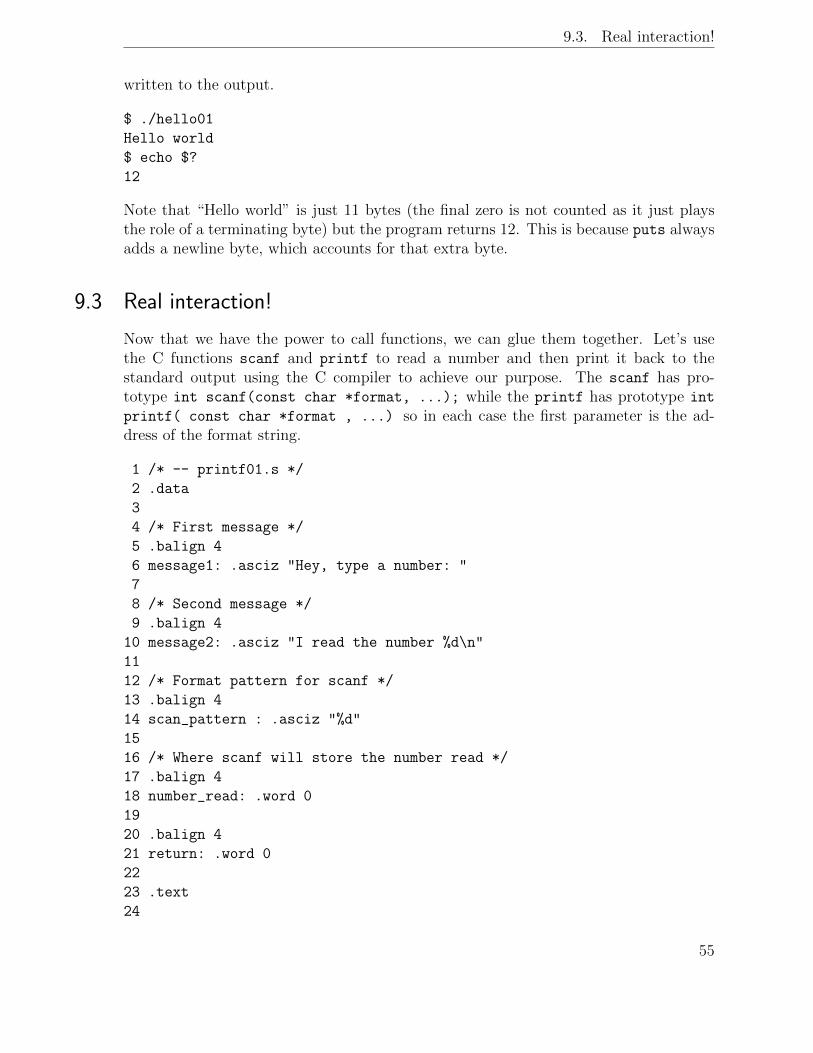
9.3. Real interaction!
written to the output.
$ ./hello01
Hello world
$ echo $?
12
Note that “Hello world” is just 11 bytes (the final zero is not counted as it just playsthe role of a terminating byte) but the program returns 12. This is because puts alwaysadds a newline byte, which accounts for that extra byte.
9.3 Real interaction!
Now that we have the power to call functions, we can glue them together. Let’s usethe C functions scanf and printf to read a number and then print it back to thestandard output using the C compiler to achieve our purpose. The scanf has pro-totype int scanf(const char *format, ...); while the printf has prototype int
printf( const char *format , ...) so in each case the first parameter is the ad-dress of the format string.
1 /* -- printf01.s */
2 .data
3
4 /* First message */
5 .balign 4
6 message1: .asciz "Hey, type a number: "
7
8 /* Second message */
9 .balign 4
10 message2: .asciz "I read the number %d\n"
11
12 /* Format pattern for scanf */
13 .balign 4
14 scan_pattern : .asciz "%d"
15
16 /* Where scanf will store the number read */
17 .balign 4
18 number_read: .word 0
19
20 .balign 4
21 return: .word 0
22
23 .text
24
55

9. Functions
25 .global main
26 main:
27 ldr r1, =return @ r1 <- &return
28 str lr, [r1] @ *r1 <- lr ; save return address
29
30 ldr r0, =message1 @ r0 <- &message1
31 bl printf @ call to printf
32
33 ldr r0, =scan_pattern @ r0 <- &scan_pattern
34 ldr r1, =number_read @ r1 <- &number_read
35 bl scanf @ call to scanf
36
37 ldr r0, =message2 @ r0 <- &message2
38 ldr r1, =number_read @ r1 <- &number_read
39 ldr r1, [r1] @ r1 <- *r1
40 bl printf @ call to printf
41
42 ldr r0, =number_read @ r0 <- &number_read
43 ldr r0, [r0] @ r0 <- *r0
44
45 ldr lr, =return @ lr <- &return
46 ldr lr, [lr] @ lr <- *lr
47 bx lr @ return from main using lr
48
49 /* External */
50 .global printf
51 .global scanf
In this example we will ask the user to type a number and then we will print it back.We also return the number in the error code, so we can check twice if everything goes asexpected. For the error code check, make sure your number is lower than 255 (otherwisethe error code will show only its lower 8 bits).
$ ./printf01 ; echo $?
Hey, type a number: 124<CR>
I read the number 124
124
9.4 Our first function
Let’s define our first function. We will extend the previous example by multiplying thenumber by 5.
14 .balign 4
56

9.4. Our first function
15 return2: .word 0
16
17 .text
18
19 /* mult_by_5 function */
20 mult_by_5:
21 ldr r1, =return2 @ r1 <- &return2
22 str lr, [r1] @ *r1 <- lr
23
24 add r0, r0, r0, LSL #2 @ r0 <- r0 + 4*r0
25
26 ldr lr, =return2 @ lr <- &return2
27 ldr lr, [lr] @ lr <- *lr
28 bx lr @ return to main using lr
This function will need another “return” variable like the one main uses. But this isonly for the sake of the example. Actually this function does not call another function.When that happens it does not need to keep lr as no bl or blx instruction is goingto modify it. If the function wanted to use lr as the general purpose register r14, theprocess of keeping the value would then be mandatory.
As you can see, once the function has computed the value, it is enough to keep it in r0.In this case it was pretty easy and a single instruction was enough.
The whole example follows.
1 /* -- printf02.s */
2 .data
3
4 .balign 4 @ First message
5 message1: .asciz "Hey, type a number: "
6 .balign 4 @ Second message
7 message2: .asciz "%d times 5 is %d\n"
8 .balign 4 @ Format pattern for scanf
9 scan_pattern: .asciz "%d"
10 .balign 4 @ Where scanf will store the number read
11 number_read: .word 0
12 .balign 4
13 return: .word 0
14 .balign 4
15 return2: .word 0
16
17 .text
18
19 /* mult_by_5 function */
57

9. Functions
20 mult_by_5:
21 ldr r1, =return2 @ r1 <- &return2
22 str lr, [r1] @ *r1 <- lr
23
24 add r0, r0, r0, LSL #2 @ r0 <- r0 + 4*r0
25
26 ldr lr, =return2 @ lr <- &return2
27 ldr lr, [lr] @ lr <- *lr
28 bx lr @ return to main using lr
29
30 .global main
31 main:
32 ldr r1, =return @ r1 <- &return
33 str lr, [r1] @ *r1 <- lr
34
35 ldr r0, =message1 @ r0 <- &message1
36 bl printf @ call to printf
37
38 ldr r0, =scan_pattern @ r0 <- &scan_pattern
39 ldr r1, =number_read @ r1 <- &number_read
40 bl scanf @ call to scanf
41
42 ldr r0, =number_read @ r0 <- &number_read
43 ldr r0, [r0] @ r0 <- *r0
44 bl mult_by_5
45
46 mov r2, r0 @ r2 <- r0
47 ldr r1, =number_read @ r1 <- &number_read
48 ldr r1, [r1] @ r1 <- *r1
49 ldr r0, =message2 @ r0 <- &message2
50 bl printf @ call to printf
51
52 ldr lr, =return @ lr <- &return
53 ldr lr, [lr] @ lr <- *lr
54 bx lr @ return from main using lr
55
56 /* External */
57 .global printf
58 .global scanf
Notice lines 46 to 49. There we prepare the call to printf which receives three pa-rameters: the format and the two integers referenced in the format. We want the firstinteger be the number entered by the user. The second one will be that same numbermultiplied by 5. After the call to mult by 5, r0 contains the number entered by the
58

9.5. Unified Assembler Language
user multiplied by 5. We want it to be the third parameter so we move it to r2. Thenwe load the value of the number entered by the user into r1. Finally we load in r0 theaddress to the format message of printf. Note that here the order of preparing thearguments of a call is not relevant as long as the values are correct at the point of thecall. We use the fact that we will have to overwrite r0, so for convenience we first copyr0 to r2.
$ ./printf02
Hey, type a number: 1234<CR>
1234 times 5 is 6170
9.5 Unified Assembler Language
As we write functions in the future, we will find that an efficient programming techniqueis to divide up the processes we wish to encode into individual functions that perform, ifpossible, just one of the needed operations. We can then test each part of the programseparately and when we are done have many useful, already tested, functions to use inother programs. This technique is called Functional Programming.
One problem arises when we combine many well-tested functions into one larger pro-gram: repeated use of the same label. Looking ahead we see programs with loops andoften the label loop:. Other common labels are exit:, error:, and next:. If we usethe same label in different functions, we will get an assembler error.
A modern syntax called Unified Assembler Language (UAL) allows for numerical labelsthat may be repeated throughout a program.
The syntax is to add the directive .syntax unified as in the following trivial example:
/* -- numericalLabels.s */
.global main /* entry point must be global */
.syntax unified /* modern syntax (UAL=Unified Assembler Language) */
.text
main: /* This is main */
push {r4, lr}
ldr r0, =message1
bl puts
b 1f /* Goto the first label 1 forward */
b 2f /* Goto the first label 2 forward */
1:
ldr r0, =message2
bl puts
1:
mov r0, 43 /* The # is optional in UAL */
59

9. Functions
pop {r4, pc} /* Return from main */
2:
ldr r0, =errmessage
bl puts
b 1b /* Goto the first label 1 backward */
.data
message1: .asciz "Numerical Label Test\n"
message2: .asciz "Success\n"
errmessage: .asciz "Failure!\n"
.global puts
Projects
1. Simplify the rest of the comments in the above example.
2. Write some other simple functions and test them. In particular, include somefunctions that operate on strings (Section 8.6).
3. Interchange lines 5 and 8 in hello01.s and show that there is no need for extraalignment. Does this give a general rule for more efficient coding? Can you thinkof any disadvantages of doing that?
4. Look up details of the prototypes for such functions as printf and scanf. Justifywhat is placed in the registers r0 and r1.
5. There are many other C functions we may use in the same way as printf andscanf. Look up their prototypes and write simple programs using them.
6. The .data sections in printf01.s and printf02.s have many unnecessary .align
statements. Rewrite them without any such statements. [Hint: .word before.asciz.]
7. Try out the UAL syntax and look up more information about it.
60
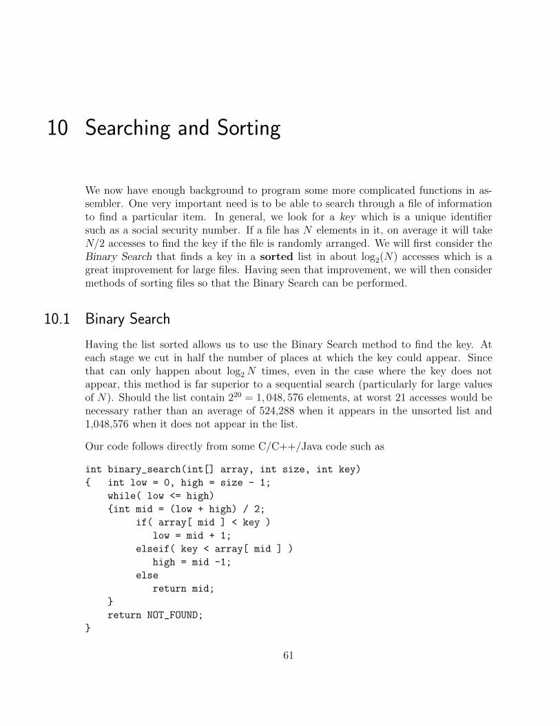
10 Searching and Sorting
We now have enough background to program some more complicated functions in as-sembler. One very important need is to be able to search through a file of informationto find a particular item. In general, we look for a key which is a unique identifiersuch as a social security number. If a file has N elements in it, on average it will takeN/2 accesses to find the key if the file is randomly arranged. We will first consider theBinary Search that finds a key in a sorted list in about log2(N) accesses which is agreat improvement for large files. Having seen that improvement, we will then considermethods of sorting files so that the Binary Search can be performed.
10.1 Binary Search
Having the list sorted allows us to use the Binary Search method to find the key. Ateach stage we cut in half the number of places at which the key could appear. Sincethat can only happen about log2N times, even in the case where the key does notappear, this method is far superior to a sequential search (particularly for large valuesof N). Should the list contain 220 = 1, 048, 576 elements, at worst 21 accesses would benecessary rather than an average of 524,288 when it appears in the unsorted list and1,048,576 when it does not appear in the list.
Our code follows directly from some C/C++/Java code such as
int binary_search(int[] array, int size, int key)
{ int low = 0, high = size - 1;
while( low <= high)
{int mid = (low + high) / 2;
if( array[ mid ] < key )
low = mid + 1;
elseif( key < array[ mid ] )
high = mid -1;
else
return mid;
}
return NOT_FOUND;
}
61

10. Searching and Sorting
Since the input of the values is not significant in this example, we will “hard-wire” intoour code the list of integers using the .word directive. The line
array: .word 2,5,11,23,47,95,191,383,767,998
both reserves 10 words in memory labeled by the name “array”, but also initializes thosewords to the given values.
1 @ BinarySearch.s
2 @
3 @ Demonstrates binary search on a fixed list of integers
4 .data @ Data declaration section
5 return: .word 0
6 array: .word 2,5,11,23,47,95,191,383,767,998
7 num_read: .word 0
8 prompt: .asciz "\nInsert integer key (key < 0 to quit): "
9 scanFMT: .asciz "%d" @ Format pattern for scanf
10 echo: .asciz "\nYou entered: %d\n"
11 ymsg: .asciz "\nKey was found at position %d\n"
12 nmsg: .asciz "\nKey not found! a near index is: %d\n"
13
14 .text @ Start of code section
15 .global main
16 main:
17 ldr r1, =return @ r1 <- &return
18 str lr, [r1] @ *r1 <- lr save return address
19
20 input:
21 ldr r0, =prompt @ r0 <- &prompt
22 bl puts @ Print prompt
23
24 ldr r0, =scanFMT @ r0 <- &scanFMT
25 ldr r1, =num_read @ r1 <- &num_read
26 bl scanf @ Call to scanf; puts value in num_read
27 @echo
28 ldr r0, =echo
29 ldr r1, =num_read
30 ldr r1, [r1]
31 bl printf @ echo the key
32
33 @check sentinal
34 ldr r1, =num_read @ r1 <- &num_read
35 ldr r1, [r1] @ r1 <- *r1
36 cmp r1, #0 @ Look for sentinal (negative)
37 blt exit @ quit if num_read is negative
62
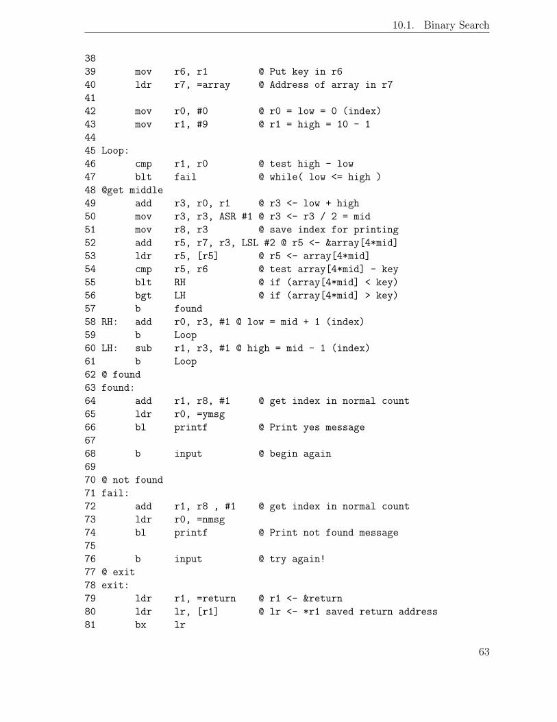
10.1. Binary Search
38
39 mov r6, r1 @ Put key in r6
40 ldr r7, =array @ Address of array in r7
41
42 mov r0, #0 @ r0 = low = 0 (index)
43 mov r1, #9 @ r1 = high = 10 - 1
44
45 Loop:
46 cmp r1, r0 @ test high - low
47 blt fail @ while( low <= high )
48 @get middle
49 add r3, r0, r1 @ r3 <- low + high
50 mov r3, r3, ASR #1 @ r3 <- r3 / 2 = mid
51 mov r8, r3 @ save index for printing
52 add r5, r7, r3, LSL #2 @ r5 <- &array[4*mid]
53 ldr r5, [r5] @ r5 <- array[4*mid]
54 cmp r5, r6 @ test array[4*mid] - key
55 blt RH @ if (array[4*mid] < key)
56 bgt LH @ if (array[4*mid] > key)
57 b found
58 RH: add r0, r3, #1 @ low = mid + 1 (index)
59 b Loop
60 LH: sub r1, r3, #1 @ high = mid - 1 (index)
61 b Loop
62 @ found
63 found:
64 add r1, r8, #1 @ get index in normal count
65 ldr r0, =ymsg
66 bl printf @ Print yes message
67
68 b input @ begin again
69
70 @ not found
71 fail:
72 add r1, r8 , #1 @ get index in normal count
73 ldr r0, =nmsg
74 bl printf @ Print not found message
75
76 b input @ try again!
77 @ exit
78 exit:
79 ldr r1, =return @ r1 <- &return
80 ldr lr, [r1] @ lr <- *r1 saved return address
81 bx lr
63

10. Searching and Sorting
82
83 /* External */
84 .global puts
85 .global printf
86 .global scanf
As often happens in moving from C/C++/Java to assembler, we must take specialpains to distinguish between indexes in the high level language and memory addresses(4 bytes to each word). In particular, in line 52 we shift left two places in order tomultiply by four thus counting in words instead of bytes. In addition, we have to watchfor alignment problems.
10.2 Insertion Sort
There are many algorithms for sorting arrays. Details can be found in any Data Struc-tures text. The “best” ones run in asymptotic time proportional to N log2N , whereN is the size of the array. That is, as N gets large, the time to sort the data growsas a constant times the factor N log2N . The criteria for being “best”, however, differwidely. One can consider the worst case or the average case or other situations. Infact the entire idea of “best” is rather meaningless when the answer is given in terms ofasymptotic time since real data sets, while large, are not infinite.
A particular example of a sorting algorithm that works well for small data sets is theinsertion sort. While its worst case behavior grows as N2 (as does its average casebehavior), for sets which are small its simplicity makes it better than complicated al-gorithms that require extensive machinery to work and the corresponding extra timeneeds to be amortized over large data sets to achieve their purported N log2N behavior.In fact, insertion sort will achieve a performance proportional to N if the data happensto be almost sorted already (which is often the case).
Here is a complete program that takes input from the keyboard for a change, sorts itusing the insertion sort algorithm, and then prints out the sorted array:
/* -- isort.s **********************
* Demonstrates insertion sort *
***********************************/
.text
.global main
main:
@@@@@@@@@@@@@@@@@ INITIALIZE
ldr r7, =return @ get ready to save
str lr, [r7] @ link register for return
mov r6, #0 @ keep count in r6
ldr r4, =array @ keep constant &array in r4
64

10.2. Insertion Sort
@@@@@@@@@@@@@@@@@ INPUT
input:
ldr r0, =prompt
bl puts
ldr r0, =scanFMT @ r0 <- &scan format
ldr r1, =number @ r1 <- &number
bl scanf @ call to scanf
ldr r1, =number
ldr r1, [r1]
cmp r1, #0 @ look for sentinal (negative)
blt isort @ goto isort function
add r0, r4, r6, LSL #2 @ r0 <- &array[4*count]
str r1, [r0] @ array[4*count] <- number
add r6, r6, #1 @ count = count + 1
b input
@@@@@@@@@@@@@@@@@ ISORT
/*
@@ sort the integers
@ C/C++/Java Code:
@ null insertion(int[] a, int n)
@ { for (int i = 1; i < n; i++)
@ { temp = a[i];
@ j = i-1;
@ while (j >= 0 && temp < a[j])
@ { a[j+1] = a[j];
@ j = j-1;
@ }
@ a[j+1] = temp;
@ }
@ }
@@
*/
isort:
mov r0, r4 @ r0 <- &array (a)
mov r1, r6 @ r1 <- count = length (n)
@
mov r2, #1 @ i = 1
iloop: @ for-loop as while loop
cmp r2, r1 @ i - n
bge iloopend @ i >= n => loopend
65

10. Searching and Sorting
add r10, r0, r2, LSL #2 @ temp = &array[4*i]
ldr r10, [r10] @ temp = array[4*i]
sub r3, r2, #1 @ j = i - 1
jloop: @ while-loop
cmp r3, #0 @ j >= 0 ?
blt jloopend
add r9, r0, r3, LSL #2 @ r9 <- &array[4*j]
ldr r9, [r9] @ r9 <- array[4*j]
cmp r10, r9 @ temp < array[4*j] ?
bge jloopend
add r8, r0, r3, LSL #2
add r8, r8, #4 @ r8 <- &array[4*(j+1)]
str r9, [r8] @ a[j+1] <- a[j]
sub r3, r3, #1 @ j <- j - 1
b jloop
@ end jloop
jloopend:
add r3, r3, #1 @ j <- j+1
add r8, r0, r3, LSL #2 @ r8 <- &array[4*(j+1)]
str r10, [r8] @ a[j+1] <- temp
add r2, r2, #1 @ i++
b iloop
@ end iloop
iloopend:
@ end isort
@@@@@@@@@@@@@@@@ OUTPUT
output:
ldr r0, =result
bl puts
mov r5, #0 @ r5 counter
ploop: cmp r6, r5 @ n - counter
ble exit @ done printing
add r3, r4, r5, LSL #2 @ r3 <- &array[4*counter]
ldr r1, [r3] @ r1 <- array[4*counter]
ldr r0, =printFMT @ r0 <- &print format
bl printf
add r5, r5, #1 @ n++
b ploop
@@@@@@@@@@@@@@@@ EXIT
exit:
mov r0, r6 @ r0 = r6 return code = n
ldr r1, =return @ r1 <- &return
ldr lr, [r1] @ lr <- *r1 saved return address
bx lr
66

10.3. Random Numbers
@@@@@@@@@@@@@@@@@
.data
number: .word 0 @ place to hold input number
array: .space 100 @ room for 25 integers = 100 bytes
return: .word 0 @ place for return address of main
prompt: .asciz "Input a positive integer (negative to quit): "
result: .asciz "Sorted, those integers are: \n"
scanFMT: .asciz "%d"
printFMT: .asciz " %d\n"
@@@@@@@@@@@@@@@@@
/* External */
.global printf
.global scanf
.global puts
The actual assembler code follows the C/C++/Java code rather closely. Again, themost frequent error in this type of program is to confuse indices with addresses. Inparticular, when using integer data from an array, one must carefully watch for placeswhere an increment or decrement must be 4 (bytes) rather than 1 (word) as in i+ +; ,i+ = 1; , or i = i+ 1; .
Notice how the inclusion of shifts in ARM instructions allows for a easy change fromindex to address (multiple of four).
10.3 Random Numbers
Simulations are an important part of system design. Before building a million dollarpiece of equipment, such as a switching network, it is customary to write a computerprogram that would simulate the operation of the device to see if it has a chance ofsatisfying the constraints imposed on it. For the example of a switching network thatwould mean simulate the arrival of millions of calls at various times and see if the systemseems to handle the load. For this purpose, large numbers of “random” numbers mustbe generated to simulate the “random” arrival of calls.
Let us generate an array of “random” numbers that might be used as test data for someother program. For more information about “random” numbers, see Knuth, Chapter 3(Volume 2) and the Projects. Here is some code:
/* -- rand.s
rand.s gives us an array of 100 pseudo-random numbers
in the range 0 <= n < 100 based on Knuth’s advice.
X[n+1] <- (aX[n] + c) mod m
67

10. Searching and Sorting
using m = 2^16 = 65536 which works on a 16-bit machine well
using a = 32445 so that a mod 8 = 5 and 99m/100 > a > m/100
using c = 1
using X0 = 31416 in r0 as seed (could be input)
*/
.text
.global main
main:
ldr r1, =return @ save return address
str lr, [r1]
/* ldr r0, #31416 @ X0 - initialized (could be input) */
mov r0, #0x7a
mov r0, r0, LSL #8
add r0, r0, #0x68 @ X0 = r0 = 0x7a68 = 31416
/* ldr r4, #32445 @ a - initialized */
mov r4, #0x7e
mov r4, r4, LSL #8
add r4, r4, #0xbd @ a = r4 = 0x7ebd = 32445
/* ldr r5, #0x0000FFFF @ mask to do modulo (m-1) - initialized */
mov r5, #0xFF
mov r5, r5, LSL #8
add r5, r5, #0xFF @ mask = m-1 = 0x0000FFFF
ldr r6, #396 @ counter - initialized 4*100-4 for 100 ints
ldr r7, #100 @ limit - initialized so values 0-99
Loop: @ while counter < 100
cmp r6, #0 @ check counter
blt Exit @ Stop when counter passes zero
mul r0, r0, r4 @ X = aX (mul works like this)
add r0, #1 @ now X = aX+c
and r0, r0, r5 @ now X = (aX+c) mod m
mov r8, r0 @ save X in r8 temporarily
lsr a0, a0, 8 @ divide by 256 (use upper 8 bits)
cmp a0, r7 @ check size
bge Loop @ only want those < 100
ldr r0, =format
mov r1, r8 @ prepare to print
bl printf
@Store
mov r0, r8 @ put X back
ldr r1, =list @ prepare to store
str r0, r1, [r6 -#4] @ store and then decrement counter
@End_of_Loop
68

10.4. More Debugging
b Loop
Exit:
ldr lr, =return
lrd lr, [lr] @ standard return to OS
bx lr
@
.data
list: .space 400 @ room for 100 integers
return: .word 0 @ save return address
format: .asciz " %d "
@
/* External */
.global printf
When we run this code we find 100 integers stored in array in the reverse order to whichthey were printed (for no obvious reason). While they may look somewhat “random”,they obviously cannot be truly random numbers since we will get exactly the sameresults every time we run this code! Again it is suggested that a careful reading ofKnuth’s material would be helpful and will justify a recommendation that any randomnumber generator a programmer uses (including those in expensive packages) should betested as much as possible.
Note that the loads during the initialization of main are carried out in three steps ratherthan the commented out one instruction. If one tries to assemble the obvious instructionldr r0, #31416, one gets an error message of some kind. On the Raspberry Pi it notonly gives the error message but also explains what number (in hex) it was unable to putin the part of the ldr - immediate machine instruction that stores the number. Withthe three instructions shown, we can obtain the desired result. You will investigateimmediate operands in a project.
10.4 More Debugging
Now that our programs are much more complicated, it is harder and harder to debugthem. There are a few additional helpful things gdb can do to assist us.
For example, the gdb command x/Nuf expression, where x stands for eXamine, willdisplay the contents of N units (u) of memory (where units could be b for byte or w
for word - four bytes) and f gives the format (which could be x for hexadecimal, c forcharacter, u for unsigned decimal, and some others) at the location decribed by theexpression.
Another importand help is the ability to set breakpoints that are locations at whichexecution will stop and wait for the user to do whatever will give them informationabout the registers and memory at that point of the program. They are set by the
69

10. Searching and Sorting
command break line or break function (and other methods) where the line is aline number from the original program and function is a label.
We now see why, in Chapter 1, we called on the assembler as with the parameter -g.That asked the assembler to keep all the debugging information available for gdb to beable to work with the original source code.
Projects
1. The isort.s code has been written in a form where it is obvious that the actualsorting code could have been separated out as a function taking the address of thearray and its length as parameters (in r0 and r1). Rewrite the code in that way.
2. Looking at the ASCII table in Appendix A, notice the values of the differentcharacters. Modify the isort.s code to act on the characters in a string.
3. There are many obvious inefficiencies in the programs given as examples in thischapter. Improve some of the obvious ones.
4. Rewrite rand.s so that it takes input from the user as the first “seed”. Run manytests of the rand program with different seeds.
5. Expand the usefulness of rand by allowing the user to pick the range of valuesreturned by the program and also how many values it returns.
6. Save the results from rand by calling the program using ./rand > data.dat andwork on the file data.dat that is created.
7. Make the data file data.dat the input to the isort program by calling it with./isort < data.dat > sorted.dat and check the results in the file sorted.dat.Note that you must append a negative number to the end of data.dat to signalthe end of input to isort.
8. Practice using gdb to watch what is an array as the program runs. Set somebreakpoints to get snapshots of what is in the various registers as the programprogresses. Note that labels are treated a function names by the debugger.
9. Try other three instruction loads similar to those used in rand.s. Using gdb,watch the behavior of the memory locations.
10. Investigate how immediate operands are formed by looking at detailed documen-tation.
70
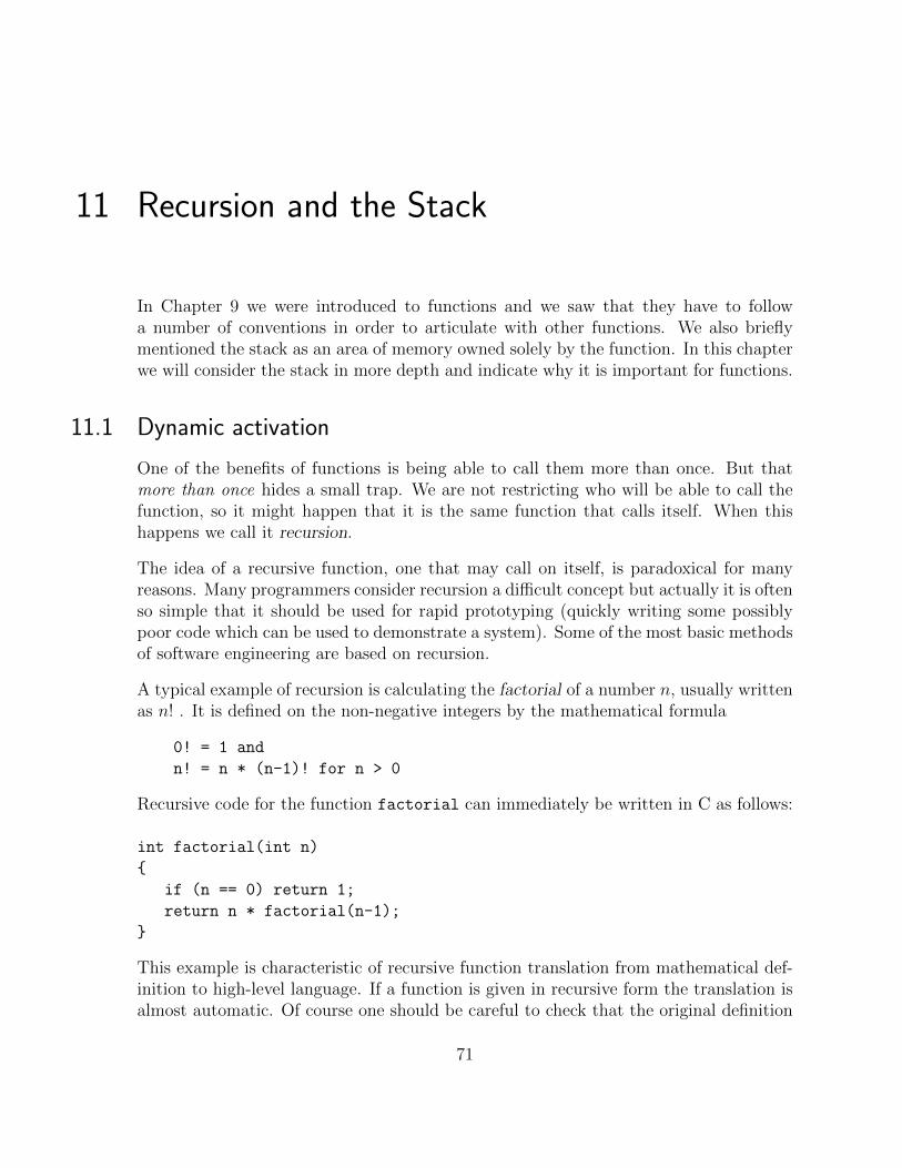
11 Recursion and the Stack
In Chapter 9 we were introduced to functions and we saw that they have to followa number of conventions in order to articulate with other functions. We also brieflymentioned the stack as an area of memory owned solely by the function. In this chapterwe will consider the stack in more depth and indicate why it is important for functions.
11.1 Dynamic activation
One of the benefits of functions is being able to call them more than once. But thatmore than once hides a small trap. We are not restricting who will be able to call thefunction, so it might happen that it is the same function that calls itself. When thishappens we call it recursion.
The idea of a recursive function, one that may call on itself, is paradoxical for manyreasons. Many programmers consider recursion a difficult concept but actually it is oftenso simple that it should be used for rapid prototyping (quickly writing some possiblypoor code which can be used to demonstrate a system). Some of the most basic methodsof software engineering are based on recursion.
A typical example of recursion is calculating the factorial of a number n, usually writtenas n! . It is defined on the non-negative integers by the mathematical formula
0! = 1 and
n! = n * (n-1)! for n > 0
Recursive code for the function factorial can immediately be written in C as follows:
int factorial(int n)
{
if (n == 0) return 1;
return n * factorial(n-1);
}
This example is characteristic of recursive function translation from mathematical def-inition to high-level language. If a function is given in recursive form the translation isalmost automatic. Of course one should be careful to check that the original definition
71

11. Recursion and the Stack
is correct and should note restrictions on the type and range of input variables. In ourfactorial example the function is only correctly defined for non-negative integers.
A recursive definition of a function always includes some base cases which, for somereason, are so trivial that their values are known or can be calculated without furtherrecursion. The recursive cases, on the other hand, must make some progress toward thebase cases. This means that the arguments for the recursive call are usually smaller insome sense (possibly smaller sets rather than always smaller integers). All our exampleswill be such that they are independent of the language we use.
Note that there is only one function factorial, but it may be called several times. Forinstance: factorial(3) → factorial(2) → factorial(1) → factorial(0), where→ means “calls”. A function, thus, is dynamically activated each time it is called. Thespan of a dynamic activation goes from the point where the function is called until itreturns. At a given time, more than one function can be dynamically activated. Thewhole dynamic activation set of functions includes the current function and the dynamicactivation set of the function that called it (the current function).
We now have a function that calls itself. That would not be a problem if it weren’t forthe rules that a function must observe. Let’s quickly recall them.
• Only r0, r1, r2 and r3 can be freely modified.
• The lr value at the entry of the function must be kept somewhere because we willneed it to leave the function (to return to the caller).
• All other registers r4 to r11 and sp may be modified but they must be restoredto their original values upon leaving the function.
In Chapter 9 we used a global variable to save lr. But if we attempted to use a globalvariable in our factorial(3) example, it would be overwritten at the next dynamic acti-vation of factorial. We would only be able to return from factorial(0) to factorial(1).After that we would be stuck in factorial(1), as lr would always have the same value.
So it looks like we need some way to keep at least the value of lr for each dynamicactivation. And not only lr; if we wanted to use registers from r4 to r11 we wouldalso need to keep them somehow for each dynamic activation. Clearly, global variableswould not be enough either. This is where the stack comes into play.
11.2 The stack
In computing, a stack is a data structure (a way to organize data that provides someinteresting properties). A stack typically has two basic operations: push informationonto the top of the stack and pop information from the top of the stack. Dependingon the context (for example, if you are not managing the stack yourself), you can only
72

11.2. The stack
access the top of the stack. In our case we will easily be able to access more elementsthan just the top. That’s because we are programming in assembler.
But, what is the stack? We already said in Chaper 9 that the stack is a region ofmemory owned solely by the function. We can now reword this a bit better: the stackis a region of memory owned solely by the current dynamic activation. And how dowe control the stack? Well, in Chapter 9 we said that the register sp stands for StackPointer. This register will contain the address of (point to) the top of the stack. Theregion of memory owned by the dynamic activation is the extent of bytes containedbetween the current value of sp and the initial value that sp had when the functionwas called. We will call that region the local memory of a function (more precisely, ofa dynamic activation of it). We will put there whatever has to be saved at entry intoa function and restored before leaving. We will also keep there the local variables of afunction (dynamic activation) which also must be removed upon exit from the function.
Our function also has to adhere to some rules when handling the stack.
The stack pointer (sp) must always be 4 byte aligned. This is absolutely mandatory.However, due to the Procedure Call Standard for the ARM architecture (AAPCS), thestack pointer will have to be 8 byte aligned, otherwise funny things may happen whenwe call what the AAPCS terms public interfaces (that is, code written by other people).The value of sp when leaving the function should be the same value it had upon enteringthe function. The first rule is consistent with the alignment constraints of ARM, wheremost times addresses must be 4 byte aligned. Due to AAPCS we will stick to the extra8 byte alignment constraint. The second rule states that, no matter how large ourlocal memory is, it will always disappear when we return from the function. This isimportant, because local variables of a dynamic activation must not have any storageassigned after that dynamic activation ends. Otherwise, repeated function calls wouldfill up the stack and cause the program to fail.
It is a convention how the stack, and thus the local memory, has its size defined. Thestack can grow upwards or downwards. If it grows upwards it means that we have toincrease the value of the sp register in order to enlarge the local memory. If it growsdownwards we have to do the opposite, the value of the sp register must be decreased byas many bytes as the size of the local storage. In our Raspberry Pi under Raspbian, thestack grows downwards, towards zero (although it never should reach zero). Addressesof local variables have very large values in the 32 bit range. They are usually close to232.
Another convention when using the stack concerns whether the sp register containsthe address of the top of the stack or some bytes above. In Raspian, the sp registerdirectly points to the top of the stack: in the memory addressed by sp there is usefulinformation.
We will now assume that the stack grows downwards and the address of top of the
73

11. Recursion and the Stack
stack must always be in sp. Clearly, to enlarge the local memory it should be enoughto decrease sp. The local memory is then defined by the range of memory from thecurrent sp value to the original value that sp had at the beginning of the function.
One register we almost always have to keep is lr. Let’s see how we can save it in thestack.
sub sp, sp, #8 @ sp <- sp - 8. This enlarges the stack by 8 bytes
str lr, [sp] @ *sp <- lr
... << Code of the function >> ...
ldr lr, [sp] @ lr <- *sp
add sp, sp, #8 @ sp <- sp + 8. This reduces the stack by 8
@ bytes, restoring the stack
@ pointer to its original value
bx lr @ return
A well behaved function may modify sp but must ensure that at the end it has thesame value it had when we entered the function. That is what we did here. We firstsubtracted 8 bytes from sp and at the end we added back the 8 bytes.
This sequence of instructions would do adequately. But maybe you remember Chapter8 and the indexing modes that you could use in load and store. Note that the first twoinstructions behave exactly like a preindexing. We first update sp and then we use sp
as the address where we store lr. This is exactly a preindex mode! Likewise for the lasttwo instructions. We first load lr using the current address of sp and then we decreasesp. This is exactly a postindex mode! The usual way to accomplish our objective is thefollowing:
str lr, [sp, #-8]! @ preindex: sp <- sp - 8; *sp <- lr
... << Code of the function >> ...
ldr lr, [sp], #+8 @ postindex; lr <- *sp; sp <- sp + 8
bx lr
Yes, those addressing modes were invented to support these sorts of things. Using asingle instruction is better in terms of code size. This may not seem relevant, but itis when we realize that the stack bookkeeping is required in almost every function wewrite!
11.3 Factorial
Let’s implement the factorial function above. First we have to learn a new instructionto multiply two numbers:
mul Rdest, Rsource1, Rsource2
74

11.3. Factorial
Note that multiplying two 32 bit values may require up to 64 bits for the result. Thisinstruction only computes the lower 32 bits. Because we are not going to use 64 bitvalues in this example, the maximum factorial we will be able to compute is 12! (13! isbigger than 232). We will not check that the entered number is lower than 13 to keep theexample simple (you are encouraged to add this check to the example, though). [Note:In versions of the ARM architecture prior to ARMv6 this instruction could not haveRdest the same as Rsource1. The GNU assembler may print a warning if you don’tuse the parameter −march = armv6.]
/* -- factorial01.s */
.data
message1: .asciz "Type a number: "
format: .asciz "%d"
message2: .asciz "The factorial of %d is %d\n"
.text
factorial: @ Assume the input n is in r0
str lr, [sp,#-4]! @ Push lr onto the top of the stack
str r0, [sp,#-4]! @ Push r0 = n onto the top of the stack
@ Note that after that, sp is 8 byte aligned
cmp r0, #0 @ Compare r0 and 0
bne is_nonzero @ if r0 != 0 then branch
mov r0, #1 @ r0 <- 1. This returns the base case
b end
is_nonzero: @ Prepare the call to factorial(n-1)
sub r0, r0, #1 @ r0 <- r0 - 1
bl factorial @ After the call r0 contains factorial(n-1)
/* Load n (that we kept in the stack) into r1 */
ldr r1, [sp] @ r1 <- *sp
mul r0, r0, r1 @ r0 <- r0 * r1 [See Project]
end:
add sp, sp, #+4 @ Discard the r0 we kept in the stack
ldr lr, [sp], #+4 @ Pop the top of the stack and put it in lr
bx lr @ Leave factorial
.globl main
main:
str lr, [sp,#-4]! @ Push lr onto the top of the stack
sub sp, sp, #4 @ Make room for one 4 byte integer on the stack
@ We will keep the number entered by the user there
75

11. Recursion and the Stack
@ Note that after that the stack is 8-byte aligned
ldr r0, =message1 @ Set &message1 as the first parameter of printf
bl printf @ Call printf
ldr r0, =format @ Set &format as the first parameter of scanf
mov r1, sp @ Set the top of the stack as the second parameter
@ of scanf
bl scanf @ Call scanf
ldr r0, [sp] @ Load the integer read by scanf into r0
@ So we set it as the first parameter of factorial
bl factorial @ Call factorial
mov r2, r0 @ Get the result of factorial and move it to r2
@ So we set it as the third parameter of printf
ldr r1, [sp] @ Load the integer read by scanf into r1
@ So we set it as the second parameter of printf
ldr r0, =message2 @ Set &message2 as the first parameter of printf
bl printf @ Call printf
add sp, sp, #+4 @ Discard the integer read by scanf
ldr lr, [sp], #+4 @ Pop the top of the stack and put it in lr
bx lr @ Leave main
Most of the code is pretty straightforward. In both functions, main and factorial, weallocate 4 extra bytes on the top of the stack. In factorial, to keep the value of r0,because it will be overwritten during the recursive call (twice, as a first parameter andas the result of the recursive function call). In main, to keep the value entered by theuser (if you recall Chapter 9 we used a global variable here).
It is important to bear in mind that in a stack, like a real stack, the last element stacked(pushed onto the top) will be the first one to be taken out from the stack (popped fromthe top). We store lr and make room for a 4 byte integer. Since this is a stack, theopposite order must be used to return the stack to its original state. We first discardthe integer and then we restore the lr. Note that this happens as well when we reservethe stack storage for the integer using a sub and then we discard such storage doing theopposite operation add.
Almost every recursive program will start with pushing onto the stack all the registersthat must be saved including, in particular, the return address. We must save lr sincethis function may call on some other (or the same) function and write over that register.Then we check to see if we have reached one of the base cases. If so, we do whateveris necessary to return the base case value. Otherwise we prepare the arguments for therecursive call. Upon return from the recursive call we just assume that the function hasperformed properly. Of course it is the programmer’s duty to ensure that fact. Finally,
76

11.4. Load and Store Multiple
we restore all the registers that were stored on the stack and return to the originalreturn address.
11.4 Load and Store Multiple
Note that the number of instructions that we need to push and pop data to and from thestack grows linearly with respect to the number of data items. Since the ARM processorwas designed for embedded systems, ARM designers devised a way to reduce the numberof instructions we need for the “bookkeeping” of the stack. These instructions are loadmultiple, ldm, and store multiple, stm.
These two instructions are rather powerful and allow a single instruction to performa lot of things. Their syntax is shown as follows. Elements enclosed in curly braces“{” and “}” (that do not appear in the actual code) may be omitted from the syntax(however, the effect of the instruction will change).
ldm addressing-mode Rbase{!}, register-set
stm addressing-mode Rbase{!}, register-set
We will consider addressing-mode later. Rbase is the base address used to load to or storefrom the register-set which is a list of registers in curly braces. All 16 ARM registersmay be specified in register-set (except pc in stm). A set of addresses is generatedwhen executing these instructions – one address per register in the register-set. Then,each register, in ascending order, is paired with one of these addresses, also in ascendingorder. This way the lowest-numbered register gets the lowest memory address, andthe highest-numbered register gets the highest memory address. Each pair (registerand address) is then used to perform the memory operation: load or store. Specifying !
means that Rbase will be updated. The updated value depends on the addressing-mode.
Note that if the registers are paired with addresses depending on their register number,then they will always be loaded and stored in the same way. For instance a register-set containing r4, r5 and r6 will always store r4 in the lowest address generated bythe instruction and r6 in the highest one. We can, though, specify what is consideredthe lowest address or the highest address. So, is Rbase actually the highest address orthe lowest address of the multiple load/store? This is one of the two aspects that iscontrolled by addressing-mode. The second aspect relates to when the address of thememory operation changes between each memory operation.
If the value in Rbase is to be considered the highest address it means that it will first de-crease Rbase as many bytes as required by the number of registers in the register-set
(that is 4 times the number of registers) to form the lowest address. Then it will load orstore each register consecutively, starting from that lowest address, always in ascendingorder of the register number. This addressing mode is called Decreasing and is specifiedusing the letter d. Conversely, if Rbase is to be considered the lowest address, thenthis is a bit easier as it can use its value as the lowest address already. We proceed as
77

11. Recursion and the Stack
usual, loading or storing each register in ascending order of their register number. Thisaddressing mode is called Increasing and is specified using the letter i.
At each load or store, the address generated for the memory operation may be updatedAfter or Before the memory operation itself. We can specify this using the letters a orb, respectively.
If we specify !, after the instruction Rbase will have the highest address generated inthe increasing mode and the lowest address generated in the decreasing mode. Thefinal value of Rbase will include the final addition or subtraction if we use a mode thatupdates After (an a mode).
So we have four addressing modes, namely: ia, ib, da and db. These addressingmodes are specified as suffixes of the stm and ldm instructions. So the full set ofnames is stmia, stmib, stmda, stmdb, ldmia, ldmib, ldmda, ldmdb. Now youmay think that this is overly complicated, but we need not use all the eight modes.Only two of them are of interest to us now.
When we push something onto the stack we actually decrease the stack pointer (becausein Raspian the stack grows downwards). More precisely, we first decrease the stackpointer as many bytes as needed before doing the actual store on that just computedstack pointer. So the appropiate addressing-mode when pushing onto the stack is stmdb.Conversely when popping from the stack we will use ldmia: we increment the stackpointer after we have performed the load.
11.5 Factorial again
Before illustrating these two instructions, we will first slightly rewrite our factorialfunction.
If you go back to the code of our factorial function, there is a moment, when computingn ∗ factorial(n− 1), where the initial value of r0 is required. The value of n was in r0
at the beginning of the function, but r0 can be freely modified by called functions. Wechose, in the example above, to keep a copy of r0 in the stack. Later, we loaded it fromthe stack into r1, just before computing the multiplication.
In our second version of factorial, we will keep a copy of the initial value of r0 in r4.But r4 is a register the value of which must be restored upon leaving a function. So wewill keep the value of r4 at the entry of the function in the stack. At the end we willrestore it back from the stack. That way we can use r4 without breaking the rules ofwell-behaved functions.
factorial:
str lr, [sp,#-4]! @ Push lr onto the top of the stack
str r4, [sp,#-4]! @ Push r4 onto the top of the stack
78

11.5. Factorial again
@ The stack is now 8 byte aligned
mov r4, r0 @ Keep a copy of the initial value of r0 in r4
cmp r0, #0 @ compare r0 and 0
bne is_nonzero @ if r0 != 0 then branch
mov r0, #1 @ r0 <- 1. This is the base case; return
b end
is_nonzero: @ Prepare the call to factorial(n-1)
sub r0, r0, #1 @ r0 <- r0 - 1
bl factorial
@ After the call r0 contains factorial(n-1)
@ Load initial value of r0 (kept in r4) into r1
mov r1, r4 @ r1 <- r4
mul r0, r0, r1 @ r0 <- r0 * r1 [See Project]
end:
ldr r4, [sp], #+4 @ Pop the top of the stack and put it in r4
ldr lr, [sp], #+4 @ Pop the top of the stack and put it in lr
bx lr @ Leave factorial
Note that the remainder of the program does not have to change. That is the cool thingabout functions.
Now pay attention to these two sequences in our new factorial version above.
str lr, [sp,#-4]! /* Push lr onto the top of the stack */
str r4, [sp,#-4]! /* Push r4 onto the top of the stack */
ldr r4, [sp], #+4 /* Pop the top of the stack and put it in r4 */
ldr lr, [sp], #+4 /* Pop the top of the stack and put it in lr */
Now, let’s replace them with stmdb and ldmia as explained in the previous section.
stmdb sp!, {r4, lr} /* Push r4 and lr onto the stack */
ldmia sp!, {r4, lr} /* Pop lr and r4 from the stack */
Note that the order of the registers in the set of registers is not relevant, but the processorwill handle them in ascending order, so we should write them in ascending order. TheGNU assembler will emit a warning otherwise. In addition, it is good programmingpractice to have them look exactly alike. Since lr is actually r14 it must go after r4.This means that our code is 100% equivalent to the previous one since r4 will end ina lower address than lr: remember our stack grows toward lower addresses, thus r4
which is in the top of the stack in factorial has the lowest address.
79

11. Recursion and the Stack
Remembering stmdb sp! and ldmia sp! may be a bit difficult. Also, given that thesetwo instructions will be relatively common when entering and leaving functions, theGNU assembler provides two mnemonics : push and pop for stmdb sp! and ldmia sp!,respectively. Note that these are not ARM instructions actually, just convenient namesthat are easier to remember (actually “macros” in the terminology of other languages).
push {r4, lr}
pop {r4, lr}
11.6 Tail-recursion
Once we have written, tested, and demonstrated some quick prototype code using recur-sion, we must turn to optimizing the code that we will actually deliver for production.The example above for calculating factorials will show us one type of optimization thatis possible.
Let us consider what return addresses are pushed onto the stack as we run a testprogram using our code. The test program will call on factorial once passing n as itsargument and we store the address of the next instruction of the test program away onthe stack. After that there will be many recursive calls on factorial with decreasingarguments from n− 1 down to 0 but in every case the return address will be the same:the instruction mov r1, r4 which follows the bl factorial within factorial. In away the repeated return addresses on the stack are little more than counters telling ushow many times the function has been called.
Each time we return from the factorial function we must then multiply the result bythe corresponding argument n. In particular, we have something else to do.
If the recursive call is the very last thing we need to do, we call the function tail-recursive. In such a case we can directly turn our recursive calls into simple jumps andso have a loop (which is faster since we would not be using the stack at all). Even whena function is not itself tail-recursive, with the aid of an auxiliary function we can oftenobtain the same benefit. Again, this technique may be used with high-level languagesjust as well. Here is our improved factorial function in C/C++/Java.
public int factorial(int n)
{
return facAux(n,1);
}
int facAux(int n, int ans)
{
if (n == 0) return ans;
facAux(n-1, n*ans);
}
80
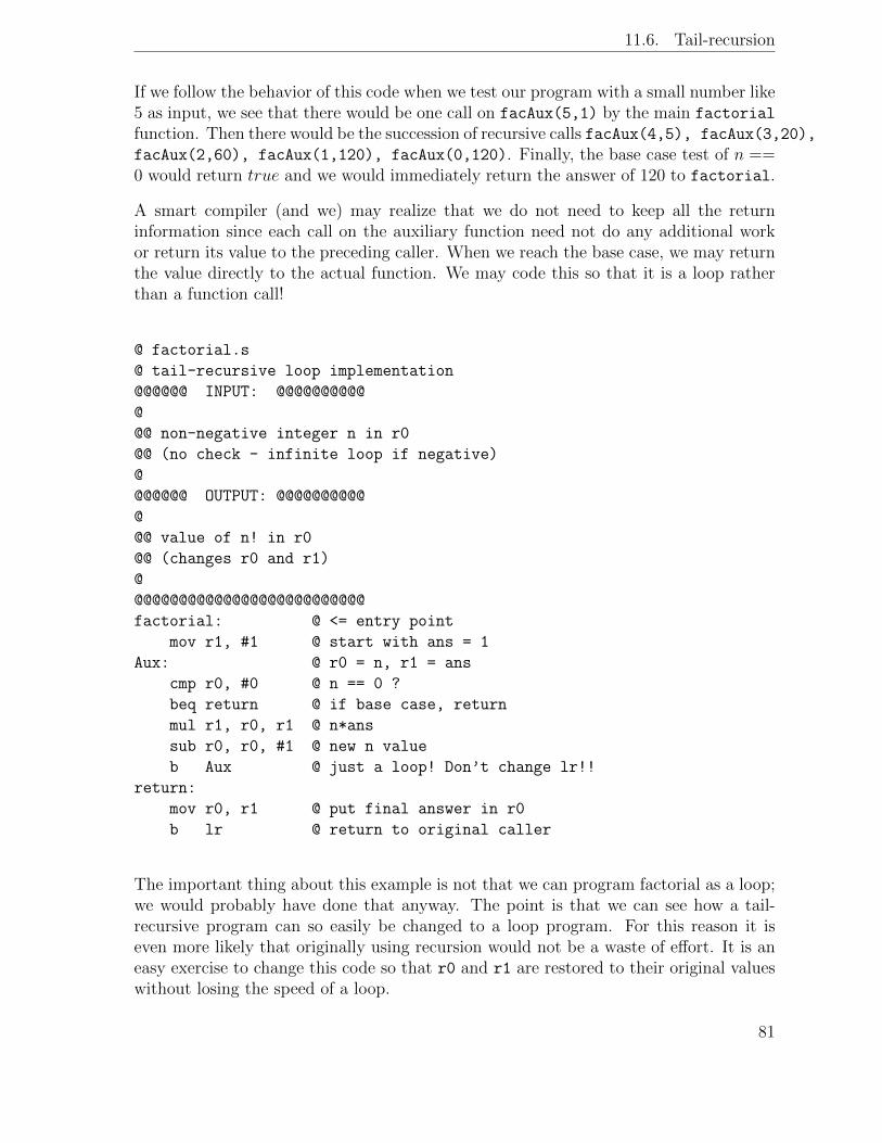
11.6. Tail-recursion
If we follow the behavior of this code when we test our program with a small number like5 as input, we see that there would be one call on facAux(5,1) by the main factorial
function. Then there would be the succession of recursive calls facAux(4,5), facAux(3,20),
facAux(2,60), facAux(1,120), facAux(0,120). Finally, the base case test of n ==0 would return true and we would immediately return the answer of 120 to factorial.
A smart compiler (and we) may realize that we do not need to keep all the returninformation since each call on the auxiliary function need not do any additional workor return its value to the preceding caller. When we reach the base case, we may returnthe value directly to the actual function. We may code this so that it is a loop ratherthan a function call!
@ factorial.s
@ tail-recursive loop implementation
@@@@@@ INPUT: @@@@@@@@@@
@
@@ non-negative integer n in r0
@@ (no check - infinite loop if negative)
@
@@@@@@ OUTPUT: @@@@@@@@@@
@
@@ value of n! in r0
@@ (changes r0 and r1)
@
@@@@@@@@@@@@@@@@@@@@@@@@@@
factorial: @ <= entry point
mov r1, #1 @ start with ans = 1
Aux: @ r0 = n, r1 = ans
cmp r0, #0 @ n == 0 ?
beq return @ if base case, return
mul r1, r0, r1 @ n*ans
sub r0, r0, #1 @ new n value
b Aux @ just a loop! Don’t change lr!!
return:
mov r0, r1 @ put final answer in r0
b lr @ return to original caller
The important thing about this example is not that we can program factorial as a loop;we would probably have done that anyway. The point is that we can see how a tail-recursive program can so easily be changed to a loop program. For this reason it iseven more likely that originally using recursion would not be a waste of effort. It is aneasy exercise to change this code so that r0 and r1 are restored to their original valueswithout losing the speed of a loop.
81
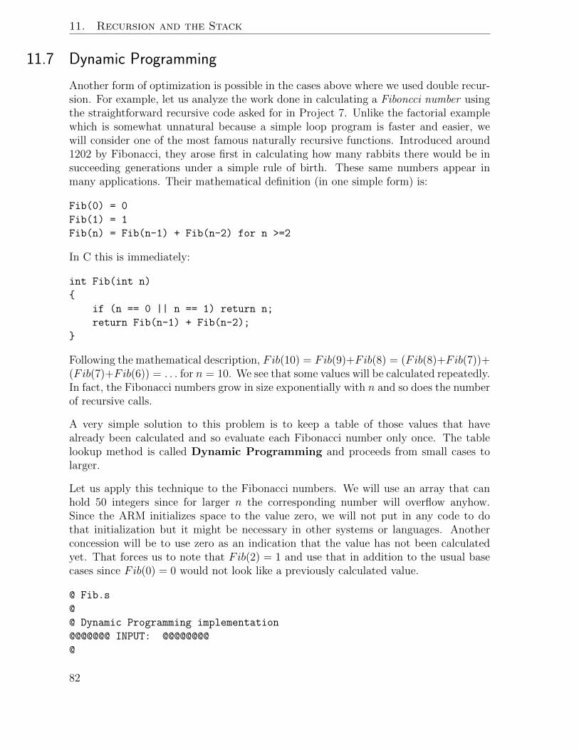
11. Recursion and the Stack
11.7 Dynamic Programming
Another form of optimization is possible in the cases above where we used double recur-sion. For example, let us analyze the work done in calculating a Fiboncci number usingthe straightforward recursive code asked for in Project 7. Unlike the factorial examplewhich is somewhat unnatural because a simple loop program is faster and easier, wewill consider one of the most famous naturally recursive functions. Introduced around1202 by Fibonacci, they arose first in calculating how many rabbits there would be insucceeding generations under a simple rule of birth. These same numbers appear inmany applications. Their mathematical definition (in one simple form) is:
Fib(0) = 0
Fib(1) = 1
Fib(n) = Fib(n-1) + Fib(n-2) for n >=2
In C this is immediately:
int Fib(int n)
{
if (n == 0 || n == 1) return n;
return Fib(n-1) + Fib(n-2);
}
Following the mathematical description, Fib(10) = Fib(9)+Fib(8) = (Fib(8)+Fib(7))+(Fib(7)+Fib(6)) = . . . for n = 10. We see that some values will be calculated repeatedly.In fact, the Fibonacci numbers grow in size exponentially with n and so does the numberof recursive calls.
A very simple solution to this problem is to keep a table of those values that havealready been calculated and so evaluate each Fibonacci number only once. The tablelookup method is called Dynamic Programming and proceeds from small cases tolarger.
Let us apply this technique to the Fibonacci numbers. We will use an array that canhold 50 integers since for larger n the corresponding number will overflow anyhow.Since the ARM initializes space to the value zero, we will not put in any code to dothat initialization but it might be necessary in other systems or languages. Anotherconcession will be to use zero as an indication that the value has not been calculatedyet. That forces us to note that Fib(2) = 1 and use that in addition to the usual basecases since Fib(0) = 0 would not look like a previously calculated value.
@ Fib.s
@
@ Dynamic Programming implementation
@@@@@@@ INPUT: @@@@@@@@
@
82

11.7. Dynamic Programming
@@ non-negative integer n in r0
@@ (no test: negative values address locations outside array)
@
@@@@@@@ OUTPUT: @@@@@@@@@@@
@
@@ nth Fibonacci number in r0
@
@@@@@@@ TO USE: @@@@@@@@@@@
@
@@ mov r0, n @ Put the n in r0
@@ bl Fib @ Returns with answer in r0
@
Fib: @ <= entry point
@ save registers
push {r4, r5, r6, lr} @ 8 byte aligned
@ check for zero
cmp r0, #0
beq return @ Fib(0) = 0
@ check FibArray for answer
mov r4, r0 @ save n in r4
mov r1, r0, LSL #2 @ take r0 = n and get r1 = 4*n
ldr r0, =FibArray @ get array address
add r0, r1, r0 @ actual location address
mov r6, r0 @ save that location address in r6
ldr r0, [r0] @ what’s there
cmp r0, #0 @ has it been calculated yet?
bne return @ if not zero, found it already
@ otherwise we have to actually do the calculation
@ adjust input parameter
sub r0, r4, #1 @ n-1 new argument
bl Fib @ first recursive call
mov r5, r0 @ save result in r5
sub r0, r4, #2 @ now use n-2 as argument
bl Fib @ second recursive call
add r0, r5, r0 @ new result
str r0, [r6] @ save it in FibArray at correct location
@ restore registers
return:
pop {r4, r5, r6, lr}
bx lr
.data
FibArray:
.word 0 @ Fib(0) = 0
.word 1 @ Fib(1) = 1
83

11. Recursion and the Stack
.word 1 @ Fib(2) = 1
.space 188 @ room for 47 more
Even on a fairly fast processor we can finally do so large a calculation that the timelag will be quite noticeable. The straight recursive Fib function will take a significantamount of time to run when given, for example, an n value of 40. With most of therecursive calls removed by Dynamic Programming, it should be instantaneous.
Projects
1. When using the mul instruction, we wrote mul r0, r0, r1. Compare that to mul
r0, r1, r0.
2. It is frequently needed to find out what is the information at the top of the stack.Write a simple function top that returns that value but does not (permanently)change the stack, using only push and pop. This shows that a built-in functiontop is not necessary but it might be available.
3. Modify the factorial function code to check for input greater than 12. Whathappens with larger values? Why?
4. Write and test a program to reverse an input list of numbers using recursion.
5. Write and test a tail-recursive function to calculate the product of two integersproduct(n,m) = n ∗ m using only addition and subtraction as if there were nomultiply hardware and it must be done in software.
6. Write and test a tail-recursive function to calculate the sum of two integerssum(n,m) = n+m using only increment (adding 1) and decrement (subtracting1) as if there were no adding hardware and it must be done in software using onlyincrement and decrement hardware.
7. (Fibonacci Numbers) Write a recursive (but not tail-recursive) assembler languageprogram to calculate the Fibonacci number of a non-negative input integer bydirect translation of the C code. How large an integer can your program handle?How slow is it?
8. (Binomial Coefficients) The number of combinations of n identical objects taken kat a time, denoted by C(n, k), can be calculated using the recursive formula givenin C/C++/Java code by
public int C(int n, int k)
{
if (n == 0 || k == 0 || k == n) return 1;
return C(n-1,k) + C(n-1,k-1); // 0 < k < n
}
84

11.7. Dynamic Programming
In our study of Discrete Mathematics we will see that C(n, k) is the kth coefficientin the expansion of the expression (x+y)n. These numbers are called the binomialcoefficients. Again it is easy to translate this directly into ARM assembly code.Write a program that prompts for n and k and returns C(n, k). Add checks forincorrect input in your code for C(n, k); return −1 if 0 ≤ k ≤ n fails in any way.
9. Using the function C(n, k) as a model, write assembler code to calculate therecursive function J defined by J(0) = 0, J(1) = 1, and
J(n) = 2nJ(n− 1)− J(n− 2)
for n ≥ 2. Assume, as usual, that r0 contains n and the answer is returned in r0.Write a driver program to print out the values of J(n) for n = 0 to n = 25. (Also,assume the values are small integers.)
10. Fix the tail-recursive version of factorial so that registers r0 and r1 are notchanged.
11. Write a “driver” program to call on our tail-recursive Fib.s program and printout values.
12. Look up the simple closed-form equation for the nth Fibonacci number.
85


12 Conditional Execution
Several times, in earlier chapters, we stated that the ARM architecture was designedwith the embedded world in mind. Although the cost of the memory becomes lowereveryday, it still may account for an important part of the budget of an embeddedsystem. The ARM instruction set has several features meant to reduce the impact ofcode size and, as we shall see, branching. One of those features is predication.
12.1 Predication
We saw in earlier chapters how to use branches in our program in order to modify theexecution flow of instructions and implement useful control structures. Branches canbe unconditional, for instance when calling a function, or conditional when we want tojump to some part of the code only when a previously tested condition is met.
Predication is related to conditional branches. What if, instead of branching to somepart of our code meant to be executed only when a condition C holds, we were able toturn off some instructions when the C condition does not hold? Consider some caselike this:
if (C)
T();
else
F();
Using predication (and with some invented syntax to express it) we could write theabove if-else statement as follows:
P = C; @ get the predicate
[P] T(); @ if P is true, do T(), otherwise, do nothing
[!P] F(); @ if P is false, do F(), otherwise, do nothing
This way we avoid branches. But, why would be want to avoid branches? Well, exe-cuting a conditional branch involves a bit of uncertainty as to what will happen in thefuture. This deserves a bit of explanation.
87

12. Conditional Execution
12.2 The pipe line of instructions
Imagine an assembly line. In that assembly line there are 5 workers, each one fullyspecialized to a single task. That assembly line executes instructions. Every instructionenters the assembly line from the left and leaves it at the right. Each worker does sometask on the instruction and passes it to the next worker to the right. Also, imagineall workers are more or less synchronized, each one ends its task in exactly 6 seconds.This means that at every 6 seconds there is an instruction leaving the assembly line, aninstruction being fully executed. It also means that at any given time there may be upto 5 instructions being processed (although not fully executed, we only have one fullyexecuted instruction at every 6 seconds).
The assembly line of instructions
Figure 12.1
The first worker fetches instructions and puts them in the assembly line. It fetchesthe instruction at the address specified by the register pc. By default, unless told, thisworker next fetches the instruction physically following the one previously fetched (thisis implicit sequencing again).
In this assembly line, suppose the worker that checks the condition of a conditionalbranch is not the first one but the third one. Now consider what happens when the firstworker fetches a conditional branch and puts it in the assembly line. The second workerwill process it and pass it to the third one. The third one will process it by checking thecondition of the conditional branch. If it does not hold, nothing happens, the branchhas no effect. But if the condition holds, the third worker must notify the first onethat the next instruction fetched should have been the instruction at the address of thebranch.
But now there are two instructions in the assembly line that should not be fully executed(the ones that were physically after the conditional branch). There are several optionshere. The third worker may pick up two stickers labeled as do nothing, and stick themon the two next instructions. Another approach would be for the third worker to tell thefirst and second workers: “Hey guys, stick a do nothing on your current instruction”.Later workers, when they see these do nothing stickers will do, naturally, nothing.This way each do nothing instruction will never be fully executed.
But by doing this, that nice property of our assembly line is gone: now we do not havea fully executed instruction every 6 seconds. In fact, after the conditional branch there
88

12.2. The pipe line of instructions
are two do nothing instructions. A program that is constantly doing branches maywell reduce the performance of our assembly line from one (useful) instruction each 6seconds to one instruction each 18 seconds. This is three times slower!
The third worker realizes that a branch is taken. Next two instructionswill get a do nothing sticker
Figure 12.2
The truth is that modern processors, including the one in the Raspberry Pi, have branchpredictors which are able to mitigate these problems: they try to predict whether thecondition will hold, so the branch is to be taken or not. Branch predictors, though,predict the future like stock brokers and weather forecasters, using the past and, whenthere is no past information, using some sensible assumptions. So branch predictorsmay work very well with relatively predictable codes but may work not so well if thecode has unpredictable behaviour.
Back to the assembly line example, it would be the first worker who attempts to predictwhether the branch will be taken or not. It is the third worker who verifies if the firstworker did the right prediction. If the first worker mispredicted the branch, then wehave to apply two stickers again and notify the first worker what is the right address ofthe next instruction. If the first worker predicted the branch right, nothing special hasto be done, which is great.
If we avoid branches, we avoid the uncertainty of whether the branch is taken or not.So it looks like that predication is the way to go. It is not a perfect answer, however.Processing a bunch of instructions that are actually turned off is not an efficient usageof a processor.
89

12. Conditional Execution
Back to our assembly line, the third worker will check the predicate. If it does not hold,the current instruction will get a do nothing sticker but in contrast to a branch, itdoes not have to notify the first worker.
So it ends, as usual, that no approach is perfect on its own. Of course we use theassembly line analogy because that is what actually happens in computer processors.Different processors have different numbers of stages in their “pipelines”, but all dodivide up the work that appears as a single instruction into stages in order to increaseperformance.
12.3 Predication in ARM
In ARM, predication is very simple to use: almost all instructions can be predicated.The predicate is specified as a suffix to the instruction name. The suffix is exactly thesame as those used in branches in Chapter 6: eq, ne, le, lt, ge and gt. Instructionsthat are not predicated are assumed to have a suffix al standing for ALways. Thatpredicate always holds and we do not write it for the sake of economy (it is validthough). You can understand conditional branches as predicated branches if you feellike it.
12.4 Collatz conjecture revisited
In Section 7.4 we implemented an algorithm that computed the length of the Collatz (orHailstone) sequence of a given number. Though not proved yet, no number has beenfound that has an infinite Collatz sequence. Given our knowledge of functions fromChapter 10, we have encapsulated the code that computes the length of the Collatzsequence in a function.
1 /* -- collatz02.s */
2 .data
3
4 message: .asciz "Type a number: "
5 scan_format: .asciz "%d"
6 message2: .asciz "Length of the Collatz sequence for %d is %d\n"
7
8 .text
9
10 collatz:
11 @ r0 contains the first argument
12 @ Only r0, r1 and r2 are modified, so
12 @ we do not need to keep anything in the stack
13 @ Since we do not do any calls, we do not have to keep lr either
14 mov r1, r0 @ r1 <- r0
90

12.4. Collatz conjecture revisited
15 mov r0, #0 @ r0 <- 0
16 collatz_loop:
17 cmp r1, #1 @ compare r1 and 1
18 beq collatz_end @ if r1 == 1 branch to collatz_end
19 and r2, r1, #1 @ r2 <- r1 & 1 (even or odd)
20 cmp r2, #0 @ compare r2 and 0
21 bne collatz_odd @ if r2 != 0 (odd) branch to collatz_odd
22 collatz_even:
23 mov r1, r1, ASR #1 @ r1 <- r1 >> 1. [r1 <- r1/2]
24 b collatz_end_loop @ branch to collatz_end_loop
25 collatz_odd:
26 add r1, r1, r1, LSL #1 @ r1 <- r1 + (r1 << 1). [r1 <- 3*r1]
27 add r1, r1, #1 @ r1 <- r1 + 1.
28 collatz_end_loop:
29 add r0, r0, #1 @ r0 <- r0 + 1
30 b collatz_loop @ branch back to collatz_loop
31 collatz_end:
32 bx lr
33
34 .global main
35 main:
36 push {lr} @ keep lr
37 sub sp, sp, #4 @ make room for 4 bytes in the stack
38 @ The stack is now 8 byte aligned
39
40 ldr r0, =message @ 1st parameter of printf: &message
41 bl printf @ call printf
42
43 ldr r0, =scan_format @ 1st parameter of scanf: &scan_format
44 mov r1, sp @ 2nd parameter of scanf:
45 address of the top of the stack
46 bl scanf @ call scanf
47
48 ldr r0, [sp] @ 1st parameter of collatz:
49 @ the value stored (by scanf) in
50 @ the top of the stack
51 bl collatz @ call collatz
52
53 mov r2, r0 @ 3rd parameter of printf:
54 @ the result of collatz
55 ldr r1, [sp] @ 2nd parameter of printf:
56 @ the value stored (by scanf) in
57 @ the top of the stack
58 ldr r0, =message2 @ 1st parameter of printf: &message2
91

12. Conditional Execution
59 bl printf
60
61 add sp, sp, #4 @ return space from stack
62 pop {lr} @ prepare to return and fix stack
63 bx lr
12.5 Adding predication
Now, let’s add some predication. There is an if-then-else construct in lines 22 to 31.There we check if the number is even or odd. If even we divide it by 2, if odd we multiplyit by 3 and add 1.
19 and r2, r1, #1 @ r2 <- r1 & 1 (even or odd)
20 cmp r2, #0 @ compare r2 and 0
21 bne collatz_odd @ if r2 != 0 (odd) branch to collatz_odd
22 collatz_even:
23 mov r1, r1, ASR #1 @ r1 <- r1 >> 1. [r1 <- r1/2]
24 b collatz_end_loop @ branch to collatz_end_loop
25 collatz_odd:
26 add r1, r1, r1, LSL #1 @ r1 <- r1 + (r1 << 1). [r1 <- 3*r1]
27 add r1, r1, #1 @ r1 <- r1 + 1
28 collatz_end_loop:
Note in line 21 that there is a bne (Branch if Not Equal) instruction. We can use thiscondition (and its opposite beq) to predicate this if-then-else construct. Instructions inthe then part will be predicated using eq, instructions in the else part will be predicatedusing ne. The resulting code is shown below.
cmp r2, #0 @ Compare r2 and 0
moveq r1, r1, ASR #1 @ if r2 == 0, r1 <- r1 >> 1. [r1 <- r1/2]
addne r1, r1, r1, LSL #1 @ if r2 != 0, r1<-r1+(r1<<1). [r1 <- 3*r1]
addne r1, r1, #1 @ if r2 != 0, r1 <- r1 + 1
As you can see, there are no labels in the predicated version. We do not branch nowso they are not needed anymore. Note also that we actually removed two branches:the one that branches from the condition test code to the else part and the one thatbranches from the end of the then part to the instruction after the whole if-then-else.This leads to a more compact code and the “pipeline” will not be stalled by possiblebranches.
12.6 Does it make any difference in performance?
Taken as it is, this program is too small to be able to accurately consider the time ittakes to run, so we modified it to run the same calculation inside the Collatz function
92

12.7. The s suffix
4,194,304 (that is 222) times. That number was chosen after some tests, so the executiondid not take so much time as to be tedious. We used the number 123 as n expecting 46steps as the answer.
It is very difficult to actually time the execution, even trying to use tools that areavailable. However, after much tribulation we obtained:
The version with branches gives the following results:
3359.953200 cpu-clock ( +- 0.01
3.365263737 seconds time elapsed ( +- 0.01
The version with predication gives the following results:
2318.217200 cpu-clock ( +- 0.01
2.322732232 seconds time elapsed ( +- 0.01
So the answer is, “yes”. In this case it does make a difference. The predicated versionruns 1.44 times faster than the version using branches. It would be bold, though, toassume that in general predication outperforms branches. Always measure your time.
12.7 The s suffix
So far, when checking the condition of an if or while, we have evaluated the conditionand then used the cmp intruction to update the cpsr. The update of the cpsr ismandatory for our conditional codes, no matter if we use branching or predication. Butcmp (and other such instructions) is not the only way to update the cpsr. In fact manyinstructions can update it.
By default an instruction does not update the cpsr unless we append the suffix s.So instead of the instruction add or sub we write adds or subs. The result of theinstruction (what is being stored in the destination register) is used to update the cpsr.Note that if we also use predication, the s follows it.
How can we use this? Well, consider this simple loop counting backwards.
/* for (int i = 100 ; i >= 0; i--) */
mov r1, #100
loop:
/* do something */
sub r1, r1, #1 @ r1 <- r1 - 1
cmp r1, #0 @ update cpsr with r1 - 0
bge loop @ branch if r1 >= 0
If we replace sub by subs then the cpsr will be updated with the result of the subtration.
93
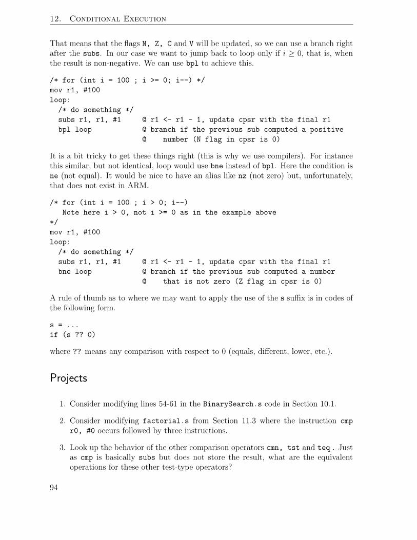
12. Conditional Execution
That means that the flags N, Z, C and V will be updated, so we can use a branch rightafter the subs. In our case we want to jump back to loop only if i ≥ 0, that is, whenthe result is non-negative. We can use bpl to achieve this.
/* for (int i = 100 ; i >= 0; i--) */
mov r1, #100
loop:
/* do something */
subs r1, r1, #1 @ r1 <- r1 - 1, update cpsr with the final r1
bpl loop @ branch if the previous sub computed a positive
@ number (N flag in cpsr is 0)
It is a bit tricky to get these things right (this is why we use compilers). For instancethis similar, but not identical, loop would use bne instead of bpl. Here the condition isne (not equal). It would be nice to have an alias like nz (not zero) but, unfortunately,that does not exist in ARM.
/* for (int i = 100 ; i > 0; i--)
Note here i > 0, not i >= 0 as in the example above
*/
mov r1, #100
loop:
/* do something */
subs r1, r1, #1 @ r1 <- r1 - 1, update cpsr with the final r1
bne loop @ branch if the previous sub computed a number
@ that is not zero (Z flag in cpsr is 0)
A rule of thumb as to where we may want to apply the use of the s suffix is in codes ofthe following form.
s = ...
if (s ?? 0)
where ?? means any comparison with respect to 0 (equals, different, lower, etc.).
Projects
1. Consider modifying lines 54-61 in the BinarySearch.s code in Section 10.1.
2. Consider modifying factorial.s from Section 11.3 where the instruction cmp
r0, #0 occurs followed by three instructions.
3. Look up the behavior of the other comparison operators cmn, tst and teq . Justas cmp is basically subs but does not store the result, what are the equivalentoperations for these other test-type operators?
94
12.7. The s suffix
4. Check whether the s suffix works on your system.
5. In addition to the operations add, sub, rsb, adc, sbc, rsc (what are theyall?), note that the mov instruction also can take an s suffix. Test out all theseARM operators. Try ldrs and see if it works.
95


13 Floating-point Numbers
So far we have only treated numbers that are integers. As we saw, their size (assuminga 32-bit 2’s-complement representation) is limited to the range of -2,147,483,648 to+2,147,483,647. For scientific purposes, even larger numbers are necessary. At theother end of the scale, very small numbers (anything less than one in absolute value!)play an equally important role. While there are many possible ways to obtain a widerrange and finer accuracy than considering only the nearest integer, we will concentrateon the representation standardized by the IEEE in 1985 and rather universally used.
13.1 IEEE-754 Standard
We should be used to what is called “scientific notation” from courses in chemistryand physics. For example, Avogadro’s number is about 6.023 × 10²³ atoms/mole andPlanck’s constant is near 6.62×10⁻²⁷ erg-seconds. The general rule in decimal notationis to pick a power of 10 for which there is exactly one non-zero digit to the left of thedecimal point. Such numbers are called normalized. Thus, from the choice of
· · · , 6023× 1020, 602.3× 10²¹, 60.23× 10²², 6.023× 10²³, 0.6023× 1024, 0.06023× 1025, · · ·
we will pick the representation used above.
The same rule will be applied to binary numbers. Each non-zero number will be writtenas a 1 to the left of the binary point, a binary fraction to its right, all multiplied bya power of two. For example, 25.75DEC would be 11001.11BIN or 1.100111BIN × 24 innormalized form. Conversions between base 10 and base 2 are quite straightforward.
The next question is how to represent these numbers in a computer. Much carefulanalysis was made about that problem and in 1985 a standard was agreed to under thedirection of the IEEE. Assuming a 32-bit word, the decision must be made as to whatthe various bits stand for. As with integers, one bit must be used to indicate the signof the number and, again, bit 31 will be used for that purpose. Now the other 31 bitsmust be assigned.
Clearly, the choice must be how many are to be assigned to the exponent of 2 andhow many (the remainder) to the binary fraction part of the number, often called themantissa. The more we allow in the exponent, the larger and smaller the numbers can
97
13. Floating-point Numbers
be. The more we allow in the mantissa, the more accurate our approximations will be.Obviously, we must trade off between range and accuracy.
The choice made by the numerical analysts was to use 8 bits for the exponent part andthe remaining 23 bits for the fractional part. Just to show how important each bit is,it was noted that every non-zero number had a single 1 to the left of the binary point.Since it must be there, it need not actually appear in the word. Thus, bits 22 downto 0 are the binary fractional part of the number with “1.” understood before it. Thusthere is the equivalent of 24 bits of accuracy rather than just 23 bits!
The choice just made affects the other 8 exponent bits from 30 down to 23, however.There are just 256 different bit patterns for those bits and again we must decide ontheir meanings. Both positive and negative exponents are needed and two’s complementrepresentation would have worked, but that wasn’t the decision for various reasons. Asunsigned integers, those 8 bits would be representations of numbers from 0 to 255. Inorder to allow negative exponents, a bias of -127 is applied to these numbers. That is,127 is subtracted from the unsigned value giving a range of exponents of the base 2 from-127 to +128.
In summary, the form of a non-zero floating-point number will be
(−1)S × 2E−127 × (1.M)
where S is the sign bit (31), E is the exponent field (30-23) as an unsigned integer, andM is the mantissa (22-0).
The number zero does not have a 1 before the binary bit and so could not be expressedin this way. Another detail was added to the rules. The unbiased exponents of 0 and255 were reserved for special cases. For example, a zero exponent is associated with thefloating-point number 0.0 and some “unnormalized” numbers smaller than those thatcan be expressed in normalized form. They have the general form
(−1)S × 20−127 × (0.M)
The exponent 11111111BIN is associated with such special values as “infinity” and“NotANumber” (0/0, for example). We will not go into these special values in any detailsince the regular numbers are interesting enough. They are the “floats” of C/C++/Java.
In case the 24-bit accuracy is not sufficient, double precision numbers were also defined.They use two consecutive words (64 bits) in a similar way. The high order bit of thefirst word is the sign bit as before. The next 11 bits of the first word are the exponent of2 biased by -1023. Finally, the remaining 52 bits consisting of the last 20 bits of the firstword and all the 32 bits of the second word are the fractional part with an understood“1.” in front as before. The unbiased exponents of 0 and 2047 are reserved for specialcases as with single precision numbers. The general form of these numbers is
(−1)S × 2E−1023 × (1.MW2)
98

13.2. Examples
where S is the sign bit (31) from the first word, E is the exponent field (30-20) fromthe first word as an unsigned integer, M is the mantissa field (19-0) of the first wordwhich is concatenated with W2, the entire second word. These are the “doubles” ofC/C++/Java.
13.2 Examples
The number 25.75DEC = 1.100111BIN × 24 described above has an exponent of 4 =131 − 127 and a fractional part of .100111BIN . Since 131DEC = 10000011BIN and thenumber is positive, the full representation of that floating-point number would be
25.75DEC = 01000001110011100000000000000000BIN = 0x41CE0000
Starting with the floating-point representation of a number such as
10111110001011000000000000000000BIN = 0xBE2C0000
we see that the sign bit is on and so the number is negative. The exponent bits formthe unsigned integer 124 and so, after subtracting 127, the exponent of 2 is -3. Puttingthe understood 1. in front of the fractional part we get 1.01011BIN , which means 1 +1/4 + 1/16 + 1/32 = 43/32. Multiplying by 2−3 = 1/8, we get the fraction 43/256 orthe decimal number −0.16796875DEC as our final answer. Our assembler can do thesecalculations for us so we will not practice many of them by hand.
An important example we should consider immediately is the decimal value 1/10 =0.1DEC . A simple method for converting base ten fractions to base two is to repeatedlydouble the fractional part of the value and take the integer part (0 or 1, obviously) asthe next bit. Thus, we obtain (0).2, (0).4, (0).8, (1).6, (1).2, (0).4, (0).8, (1).6, (1).2,(0).4, (0).8, (1).6, etc. The binary fraction, then, is
0.000110011001 . . .BIN = 2−4 × 1.10011001 . . .BIN
whick is obviously a repeating fraction. When we try to represent this number we musttruncate it to as many bits as are available. In normalized IEEE-754 form we wouldhave
+2123−127(1 + .10011001 . . .BIN) = 0011110111001100110011001100110?BIN
where the last place is in question since there must be round-off error when truncatinga repeating fraction of this type. The bit in the question mark place is a zero but thenext bit would be a one. That means that the remainder would be more than one-halfand so we should round the value to a one in the last place. Our final answer would be
0.1DEC ≈ 00111101110011001100110011001101BIN = 0x3DCCCCCD
This number is slightly more than 1/10 but 0x3DCCCCCC is slightly less than 1/10.We cannot express the simple fraction 1/10 exactly in our binary system! We have,however, exactly expressed the fraction 13421773/134217728 (check this!).
99
13. Floating-point Numbers
In many computers there are additional bits carried along with the stated 32 to improvethe accuracy of computations. That is a subject of more advanced study. For us theimportant thing is that no matter how many bits are used, there will be errors inour values since not all numbers can be exactly represented. Indeed, only at most 232
different numbers could possibly be represented with only 32 bits. Doing everything indouble precision may be more accurate (and slower), but is not the entire answer since,again, not all values can be represented.
13.3 Extremes
Since one of the reasons for using floating-point numbers rather than just integers was toextend the range of values which could be described, we will now consider exactly whatthe largest and smallest values available are. Using the 32-bit IEEE-754 standard, wemust remember that the unbiased exponents of 0 and 255 are reserved so the smallestwe may use is 1 and the largest 254.
The smallest (positive) number would have an unbiased exponent field of 00000001BIN
and a mantissa of all zeros. The true exponent of 2 would be 1-127 = -126 whilethe fractional part would be just the virtual 1. we assume present. In other words, thedecimal value of the smallest positive number would be 2−126(1.0) ≈ 1.175494351×10−38.
It is interesting to also consider what would be the very next larger positive numberthat can be represented. The unbiased exponent would still be 1 but the fraction wouldhave a 1 in the last place, corresponding to a term of 2−23. The result, then, is
2−126(1 + 2−23) = 2−126 + 2−149 ≈ 1.175494211× 10−38,
the numbers differing by about 1.401298464 × 10−45. Notice that the smallest and thenext larger number agree in their first seven digits (1175494). We would say that theyare the same to seven “significant figures.”
At the other end of the range of values, the largest positive number would have anunbiased exponent of 254 so the true exponent would be 254-127=127. The fractionalpart would have all ones and the number would look like
01111111011111111111111111111111BIN = 0x7F7FFFFF
Recognizing the positions in the fraction stand for negative powers of two, we see thatif we add one in the last or least significant position (2−23) to the number, we would geta sum of 2 (since there is already a virtual “1.” in front of the fraction). Putting thesefacts together we have the value
2127 × (2− 2−23) = 2128 − 2104 ≈ 3.402823669× 1038 − 2.028240960× 1031
and that is approximately 3.402823466× 1038. Now let us find the very next (smaller)number in this representation. It would look like 0x7F7FFFFE, differing by having a
100

13.4. Exceptions
zero in the last place. The calculation we just did tells us that the change will be thevalue of 2104 found above or about 2×1031, which is a very large number. The fact thatany number in the entire range of over 1031 reals from one number to the next must berounded-off to one of these numbers differing by so much is surprising. On the otherhand, we note that we still have the same seven significant figures as we had before!
While there can be no exact representation of all the integers between the largest andthe next largest number, it is interesting to note that every integer less than 16,777,216has an exact IEEE-754 representation. It is an exercise to show why that is true.
13.4 Exceptions
Although we now can express numbers over a very large range, it is still possible to havethe same overflow problem we had with integers. If the result of a calculation (or anyof its intermediate steps) is larger in size than the 3.402823466× 1038 we found above,the system must take some special action. As with integers, the behavior of a systemdepends on the hardware and software involved. In some cases an exception is raised(as in Java’s try-catch statements) and can be handled by special code written by theprogrammer. In other cases the hardware may automatically transfer control to code inthe operating system that may or may not allow the program to continue.
With floating-point numbers there is another problem that can arise. The result of acalculation (or, again, any of its intermediate steps) may be smaller in size than the1.175494351 × 10−38 we calculated above. If that happens, we say that underflow hasoccurred. Again the behavior of the system depends on both the hardware and thesoftware involved.
A very frustrating situation can occur when one’s program contains a loop in which bet-ter and better approximations to the correct answer are being calculated. The error termis getting smaller and smaller. On some systems the language/compiler/OS/hardwarecombination is such that if the approximation gets too good, the error term causesunderflow and the program is aborted without any way for the user to retrieve thatexcellent approximation. (See Chapter 16 for more on exceptions.)
13.5 Accuracy
Unlike integers in which their arithmetic is exact, the operations of addition, subtraction,multiplication, and division will usually yield only approximations to the correct answer.As we saw above, we cannot represent 0.1DEC exactly and so adding it to itself 10 timeswill probably not yield 1.0DEC exactly. Consider the simple for-loops in C/C++/Javapseudo-code:
for (float x = 0.0; x < 1.0; x += 0.1) {do something involving x}
101

13. Floating-point Numbers
versus
for (int i = 0; i < 10; i++) {do something involving x=i/10.0}
While the second will definitely loop ten times, the first might not! In fact, an evenmore dangerous idea is to test two float numbers for equality. While we could replacei < 10 by i != 10, the expression x != 1.0 would probably always be true and give usan infinite loop! As a general rule in C/C++/Java, never test floats for equality!
As mentioned before, we will not spend time now on hand calculations that involvefloating-point numbers since the GNU assembler actually supports them and allows usto use them quite easily. However, even before writing programs which use floating-point numbers in the next chapter, we can consider another major problem that canoccur with them.
Suppose we are doing decimal calculations involving π = 3.141592654 . . . and also a veryaccurate fractional approximation 355/113 = 3.14159292 . . . . [Note: That’s a lot betterthan 22/7.] If we actually have, as calculated above, just 7 significant digits, these twovalues would be stored as 3.141593 and 3.141593 — exactly the same! Indeed, if wewere able to store them to 8 significant figures, they would be 3.1415927 and 3.1415929.Their difference would be 0.0000002 a figure with just 1 significant digit in it!
This behavior is called catastrophic cancellation. When we take the difference betweentwo numbers of approximately the same size, we lose significant digits in the answer.The ill-conditioned Hilbert matrices are an excellent example of this problem. The nth
Hilbert matrix is defined to be
1 1/2 1/3 · · · 1/n1/2 1/3 1/4 · · · 1/(n+ 1)1/3 1/4 1/5 · · · 1/(n+ 2)
......
.... . .
...1/n 1/(n+ 1) 1/(n+ 2) · · · 1/(2n− 1)
Expanding the determinant of such a matrix we find it has n! terms, half positive andhalf negative, and all about the same size. Trying to calculate the determinant of evensmall cases of the Hilbert matrix is difficult.
A common behavior is using 22/7 = 3.142857143 . . . and keeping all those figures pastthe third when approximating π. The problem is that a computer will print out thesame large number of digits, even if most of them are meaningless. That leads peopleto believe in their accuracy quite unjustifiably.
Let us look at the simple act of adding two floating-point numbers together. If theirsizes are nearly the same, we saw above that subtracting can cause loss of precision.Now suppose that the two numbers are quite different in size and we wish to add them.Since they are assumed to be different in size, their exponents will be very different. Inorder to add them we must first shift the smaller one (with the smaller exponent) to
102

13.6. *Fixed-point Numbers
the right, thus “un-normalizing” it, until it has the same exponent as the larger. Onlythen can we add the fractional parts. That result may need renormalization but that iseasy to do. The problem is that when we shifted the smaller number right we may havelost some of the important information those lower bits contained. Obviously, if thenumbers differ by more than the seven significant decimal digits we have, the smallerwill look just like zero!
13.6 *Fixed-point Numbers
While the floating-point numbers have the advantage in range, the integers we consideredearlier had the advantage of allowing for exact calculations. Our integers in two’scomplement form are just one example of another general way in which we may representnumbers in a computer. Fixed-point numbers are used in many Digital Signal Processing(DSP) systems [but NOT the ARM processor we are studying].
Since they are not really part of our use of ARM as an example for the study of assemblerand computer architecture, we will introduce them as they would appear on a 16-bitmachine just to emphasize this point. A general notation for a fixed-point format is m.n(mQ.n and Qn are also used in the literature) where m is the number of bits (includinga sign bit) assumed to the left of the binary point and n is the number of bits to theright. Thus, m+n always equals the total number of bits available (we will use 16 here).
For negative numbers we will still use the two’s complement method of representation.Thus, the 16-bit integers may be considered fixed-point numbers with format 16.0; allsixteen bits appear before the virtual binary point. Were we to need to consider exactcalculations concerning dollars and cents, we might use the equivalent of a 14.2 formatin a decimal computer, carrying two digits after the decimal point.
In many cases, we know that our data is of absolute value less than one (sine or cosine,maybe). An interesting format for such numbers would be 1.15 (also called Q15); onesign bit and 15 fractional bits. Let us consider the details of such numbers.
The largest 16-bit positive fixed-point number expressible in 1.15 format would be0111111111111111BIN . That is, the sign bit of zero followed by a binary point andthe fractional part consisting of all ones. The value of this number would be 1–2−15 ≈.9999694824DEC , very close to 1. On the other hand, the smallest positive number wouldbe 0000000000000001BIN whose value is 2−15 ≈ .00003051757812DEC .
These numbers act like integers in that each successive number differs by exactly that2−15 we found above and their arithmetic is exact. For many purposes, particularlyin DSP calculations, fixed-point numbers fit the problem very well and the hardwareshould be made available to support such numbers and their calculations. All that wehave discussed concerning 16-bit numbers applies to our usual 32-bit numbers. A pointto notice is that there are just 65536 different 16-bit patterns and it is up to us to decidehow to interpret them.
103

13. Floating-point Numbers
Projects
1. Justify the doubling method described for converting decimal fractions to binary.
2. Express 1.0DEC in IEEE-754 form. What is the next larger number expressible inthat representation?
3. What integers can be exactly expressed in IEEE-754 form?
4. What is the decimal value of the floating-point number 0xD52C0000?
5. What are the values of the two approximations to 0.1DEC found above?
6. What are the largest and smallest positive numbers in double precision?
7. In C/C++/Java, add up the terms of the infinite series 1 + 1/2 + 1/3 + 1/4 + . . .until the partial sums no longer change. At what point did that happen? Whatvalue for the partial sum did you get? What is the correct sum of this infiniteseries? Try starting at the place you found above and adding them together inreverse order. Is the answer the same?
8. What are the largest and smallest 32-bit fixed-point numbers in 1.31(or Q31)format?
9. Calculate the determinant of some of the small cases of the Hilbert matrices.
10. Look up the new enhancements to the IEEE754-2008 requirements as used by theARM 3.
104

14 Real Computations
In the early days of computers, there was no hardware support for floating-point com-putations. If they were needed, software routines had to be written to perform anyoperations desired. The 8087 chip which was added later and served as a coprocessorto the 8088 processor in the original PC was extremely powerful and demonstrated theadvantages of having floating-point numbers fully supported in hardware. Neverthe-less, many DSP chips today, although fantastically powerful, only support fixed-pointnumbers.
The ARM processor has a floating-point coprocessor with it and so does an excellentjob of supporting such computations. As we stated several times in earlier chapters,the ARM was designed to be very flexible. We can see this in the fact that the ARMarchitecture provides a generic coprocessor interface. Manufacturers of a “system-on-a-chip” may bundle additional coprocessors. Each coprocessor is identified by a numberand provides specific instructions. For instance the Raspberry Pi SoC is a BCM2835which provides a multimedia coprocessor (which we will not discuss here).
That said, there are two standard coprocessors in the ARMv6 architecture: 10 and 11.These two coprocessors provide floating point support for single and double precision,respectively. Although the floating point instructions have their own specific names,they are actually mapped to generic coprocessor instructions targeting coprocessors 10and 11.
The ARMv6 defines a floating point subarchitecture called the Vector Floating-Point v2(VFPv2). Version 2 because earlier ARM architectures supported a simpler form callednow v1. As stated above, the VFP is implemented on top of two standarized coprocessors10 and 11. The ARMv6 does not require VFPv2 be implemented in hardware (one canalways resort to a slower software implementation). Fortunately, the Raspberry Pi 2does provide a hardware implementation of VFPv2.
14.1 VFPv2 Registers
We already know that the ARM architecture provides 16 general purpose registers r0
to r15, where some of them play special roles: r13, r14 and r15. Despite their name,these general purpose registers do not allow operating on floating point numbers in them,
105
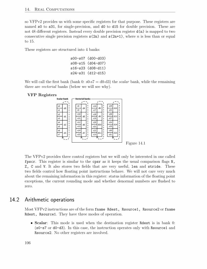
14. Real Computations
so VFPv2 provides us with some specific registers for that purpose. These registers arenamed s0 to s31, for single-precision, and d0 to d15 for double precision. These arenot 48 different registers. Instead every double precision register d(n) is mapped to twoconsecutive single precision registers s(2n) and s(2n+1), where n is less than or equalto 15.
These registers are structured into 4 banks:
s00-s07 (d00-d03)
s08-s15 (d04-d07)
s16-s23 (d08-d11)
s24-s31 (d12-d15)
We will call the first bank (bank 0: s0-s7 = d0-d3) the scalar bank, while the remainingthree are vectorial banks (below we will see why).
VFP Registers
Figure 14.1
The VFPv2 provides three control registers but we will only be interested in one calledfpscr. This register is similar to the cpsr as it keeps the usual comparison flags N,
Z, C and V. It also stores two fields that are very useful, len and stride. Thesetwo fields control how floating point instructions behave. We will not care very muchabout the remaining information in this register: status information of the floating pointexceptions, the current rounding mode and whether denormal numbers are flushed tozero.
14.2 Arithmetic operations
Most VFPv2 instructions are of the form fname Rdest, Rsource1, Rsource2 or fnameRdest, Rsource1. They have three modes of operation.
• Scalar: This mode is used when the destination register Rdest is in bank 0:(s0-s7 or d0-d3). In this case, the instruction operates only with Rsource1 andRsource2. No other registers are involved.
106

14.2. Arithmetic operations
• Vectorial: This mode is used when the destination register Rdest and Rsource2
(or Rsource1 for instructions with only one source register) are not in bank 0.In this case the instruction will operate on as many registers (starting from thegiven register in the instruction and wrapping around the bank of the register)as defined in field len of the fpscr (at least 1). The next register operated on isdefined by the stride field of the fpscr (at least 1). If wrap-around happens, noregister can be operated on twice.
• Scalar expanded (also called mixed vector/scalar): This mode is used if Rsource2(or Rsource1 if the instruction only has one source register) is in bank 0, but thedestination is not. In this case Rsource2 (or Rsource1 for instructions with onlyone source) is left fixed as the source. The remaining registers are operated on asin the vectorial case (that is, using len and stride from the fpscr).
This looks rather complicated, so let’s see some examples. Most instructions have asuffix of .f32 if they operate on single-precision and .f64 if they operate on double-precision numbers. We can add two single-precision numbers using
vadd.f32 Rdest, Rsource1, Rsource2
and two double-precision numbers using
vadd.f64 Rdest, Rsource1, Rsource2
Note also that we can use predication in these instructions (but be aware that, as usual,predication uses the flags in cpsr not in fpscr). Predication would be specified beforethe suffix as in vaddne.f32.
/* In the following examples, assume that len = 4, stride = 2 */
vadd.f32 s1, s2, s3 /* s1 <- s2 + s3. Scalar operation because
Rdest = s1 is in bank 0 */
vadd.f32 s1, s8, s15 /* s1 <- s8 + s15. Same as previous */
vadd.f32 s8, s16, s24 /* s8 <- s16 + s24
s10 <- s18 + s26
s12 <- s20 + s28
s14 <- s22 + s30
or more compactly {s8,s10,s12,s14} <-
{s16,s18,s20,s22} + {s24,s26,s28,s30}
Vectorial, since Rdest and Rsource2
are not in bank 0
*/
vadd.f32 s10, s16, s24 /* {s10,s12,s14,s8} <-
{s16,s18,s20,s22} + {s24,s26,s28,s30}
Vectorial, but note the wraparound
inside the bank after s14.
*/
107

14. Real Computations
vadd.f32 s8, s16, s3 /* {s8,s10,s12,s14} <-
{s16,s18,s20,s22} + {s3,s3,s3,s3}
Scalar expanded since Rsource2 is in bank 0
*/
14.3 Load and Store
Once we have a rough idea of how we can operate floating points in VFPv2, a questionremains: how do we load/store floating point values from/to memory? VFPv2 providesseveral specific load/store instructions.
We load/store one single-precision floating point using vldr/vstr. The address of thedatum must already be in a general purpose register, although we can apply an offsetin bytes which must be a multiple of 4 (this applies to double-precision as well).
vldr s1, [r3] @ s1 <- *r3
vldr s2, [r3, #4] @ s2 <- *(r3 + 4)
vldr s3, [r3, #8] @ s3 <- *(r3 + 8)
vldr s4, [r3, #12] @ s3 <- *(r3 + 12)
vstr s10, [r4] @ *r4 <- s10
vstr s11, [r4, #4] @ *(r4 + 4) <- s11
vstr s12, [r4, #8] @ *(r4 + 8) <- s12
vstr s13, [r4, #12] @ *(r4 + 12) <- s13
We can load/store several registers with a single instruction. In contrast to generalload/store, we cannot load an arbitrary set of registers but instead they must be asequential set of registers.
/*
Here precision can be s or d for single-precision or double-precision.
The floating-point-register-set is {sFirst-sLast} for
single-precision and {dFirst-dLast} for double-precision.
*/
vldm indexing-mode precision Rbase{!}, floating-point-register-set
vstm indexing-mode precision Rbase{!}, floating-point-register-set
The behaviour is similar to the indexing modes we saw in Chapter 8. There is an Rbaseregister used as the base address of several load/store to/from floating point registers.There are only two indexing modes: increment after and decrement before. Whenusing increment after, the address used to load/store the floating point value register isincreased by 4 after the load/store has happened. When using decrement before, thebase address is first decremented by as many bytes as floating point values are going tobe loaded/stored. Rbase is always updated by decrementing before but it is optional toupdate it by incrementing after.
108

14.4. Movements between registers
vldmias r4, {s3-s8} /* s3 <- *r4
s4 <- *(r4 + 4)
s5 <- *(r4 + 8)
s6 <- *(r4 + 12)
s7 <- *(r4 + 16)
s8 <- *(r4 + 20)
*/
vldmias r4!, {s3-s8} /* Like the previous instruction
but at the end r4 <- r4 + 24
*/
vstmdbs r5!, {s12-s13} /* *(r5 - 4 * 2) <- s12
*(r5 - 4 * 1) <- s13
r5 <- r5 - 4*2
*/
For the usual stack operations when we push onto the stack several floating point reg-isters we will use vstmdb with sp! as the base register. To pop from the stack we willuse vldmia again with sp! as the base register. Given that these instructions namesare very hard to remember we can use the mnemonics vpush and vpop, respectively.
vpush {s0-s5} /* Equivalent to vstmdb sp!, {s0-s5} */
vpop {s0-s5} /* Equivalent to vldmia sp!, {s0-s5} */
14.4 Movements between registers
Another operation that may be required is moving data between registers. Similar tothe mov instruction for general purpose registers, there is the vmov instruction. Severalmovements are possible.
We can move floating point values between two floating point registers of the sameprecision:
vmov s2, s3 /* s2 <- s3 */
vmov d3, d4 /* d3 <- d4 */
We can also move data between one general purpose register and one single-precisionregister as follows. Note, however, that the data is not converted. Only bits are copied,so be careful not to mix floating point values with integer instructions or the other wayaround.
vmov s2, r3 /* s2 <- r3 */
vmov r4, s5 /* r4 <- s5 */
Similar to the previous case but between two general purpose registers and two consec-utive single-precision registers we have:
109

14. Real Computations
vmov s2, s3, r4, r10 /* s2 <- r4
s3 <- r10 */
Finally, consider moving between two general purpose registers and one double-precisionregister. Again, note that the data are not converted.
vmov d3, r4, r6 /* Lower32BitsOf(d3) <- r4; Higher32BitsOf(d3) <- r6 */
vmov r5, r7, d4 /* r5 <- Lower32BitsOf(d4); r7 <- Higher32BitsOf(d4) */
14.5 Conversions
Sometimes we need to convert from an integer to a floating-point and the reverse. Notethat some conversions may potentially lose precision, in particular when a floating pointis converted to an integer. There is a single instruction vcvt with a suffix .T.S whereT (target) and S (source) can be u32, s32, f32 or f64 (S must be different from T).Both registers must be floating point registers, so in order to convert an integer to afloating point or a floating point to an integer value an extra vmov instruction will berequired from or to an integer register before or after the conversion. Because of this, fora moment (between the two instructions) a floating point register will contain a valuewhich is not an IEEE 754 value; bear this in mind. Here are some examples:
vcvt.f64.f32 d0, s0 /* Converts a single-precision value in s0 to a
double-precision value and stores it in d0 */
vcvt.f32.f64 s0, d0 /* Converts a double-precision value in d0 to a
single-precision value and stores it in s0 */
vmov s0, r0 /* Bit copy from integer register r0 to s0 */
vcvt.f32.s32 s0, s0 /* Converts a signed integer value in s0 to a
single-precision value and stores it in s0 */
vmov s0, r0 /* Bit copy from integer register r0 to s0 */
vcvt.f32.u32 s0, s0 /* Converts an unsigned integer value in s0 to a
single-precision value and stores in s0 */
vmov s0, r0 /* Bit copy from integer register r0 to s0 */
vcvt.f64.s32 d0, s0 /* Converts a signed integer value in r0 to a
double-precision value and stores in d0 */
vmov s0, r0 /* Bit copy from integer register r0 to s0 */
vcvt.f64.u32 d0, s0 /* Converts an unsigned integer value in s0 to a
double-precision value and stores in d0 */
110
14.6. Modifying the fpscr
14.6 Modifying the fpscr
The special register fpscr, where len and stride are set, cannot be modified directly.Instead we have to load fpscr into a general purpose register using the vmrs instruction.Then we operate on the register and move it back to the fpscr, this time using thevmsr instruction.
The value of len is indirectly stored in bits 16 to 18 of the fpscr. The value of len isnot directly stored in those bits. Instead, we have to subtract 1 before setting the bits.This is because len cannot be 0 (it does not make sense to operate 0 floating points).This way the value 000 in these bits means len = 1, 001 means len = 2, . . ., 111 meanslen = 8. The following is an example of code that sets len to 8.
/* Set the len field of fpscr to be 8 (bits: 111) */
mov r5, #7 @ r5 <- 7. 7 is 111 in binary
mov r5, r5, LSL #16 @ r5 <- r5 << 16
vmrs r4, fpscr @ r4 <- fpscr
orr r4, r4, r5 @ r4 <- r4 | r5. Bitwise OR
vmsr fpscr, r4 @ fpscr <- r4
The value of stride is indirectly stored in bits 20 to 21 of fpscr in a manner similarto len: a value of 00 in these bits means stride = 1, 01 means stride = 2, 10 meansstride = 3 and 11 means stride = 4.
14.7 Function call convention and floating-point registers
Since we have introduced new registers we should state how to use them when callingfunctions. The following rules apply for VFPv2 registers.
• Fields len and stride of fpscr are zero at the entry of a function and must bezero when leaving it.
• We can pass floating point parameters using registers s0-s15 and d0-d7. Notethat passing a double-precision after a single-precision may involve discarding anodd-numbered single-precision register (for instance we can use s0, and d1 butnote that s1 will be unused).
• All other floating point registers (s16-s31 and d8-d15) must have their valuespreserved upon leaving the function. Instructions vpush and vpop can be used forthat.
• If a function returns a floating-point value, the return register will be s0 or d0.
Finally a note about functions like printf that can take a variable number of arguments:you cannot pass a single-precision floating point to one of such functions. Only doubles
111

14. Real Computations
can be passed. So you will need to convert the single-precision values into double-precision values. Note also that usual integer registers are used (r0-r3), so you willonly be able to pass up to 2 double-precision values in registers, the remaining must bepassed on the stack. In particular for printf, since r0 contains the address of the stringformat, you will only be able to pass a single double-precision number in {r2,r3} andany others on the stack.
14.8 Printing Floating-point Numbers
We will continue to use the C function printf to print values but its behavior forfloating-point numbers is a bit different as described above. First of all, it only printsdouble-precision numbers. Since r0 contains, as before, the address of the ASCII stringgiving the format information, we will have to store the first value to be printed in{r2,r3}. Additional values to be printed must be placed on the stack as usual. Thecode for one value would be
ldr r0, =format
vmov r2, r3, Dx @ x is the number of the register holding the value
bl printf
Assembler Note
Make sure you pass the flag -mfpu=vfpv2 to the assembler as, otherwise it will notrecognize the VFPv2 instructions.
Projects
1. Try out various combinations of conversions.
2. Modify earlier programs that worked for integers so that they can handle floating-point numbers. In particular, functions in such programs as factorial andFibonacci were limited by the size of integers. How much larger values willwork if we are using floating-point numbers?
3. See Appendix C for a very long but valuable example of Matrix Multiplication forfloating-point numbers.
4. Try out various combinations of len and stride and test the results.
112

15 Pointers
In Chapter 9 we saw the basics of how to call a function. In this chapter we will covermore topics related to functions.
15.1 Passing data to functions
We already know how to call a function and pass it parameters. We also know howto return data from a function. Nevertheless, there are some issues which we have notfully solved yet.
• Passing large amounts of data
• Returning more than one piece of data
There are several ways to tackle these problems, but most of them involve pointers.Pointers are dreaded by many people who do not fully understand them, but they are acrucial part of the way computers work. That said, most of the troubles with pointersare actually related to using dynamic memory rather than the pointers themselves. Wewill not consider dynamic memory here.
15.2 What is a pointer?
A pointer is some location in memory the contents of which are simply the address of(“points to”) some location in memory.
This definition may be confusing, but we have already been using pointers in previouschapters. It is just that we usually did not name them that way. We usually talkedabout addresses and/or labels in the assembler. Consider this very simple program:
/* first_pointer.s */
.data
Number1: .word 3
.text
113

15. Pointers
.globl main
main:
ldr r0, pointerToNumber1 @ r0 <- &Number1
ldr r0, [r0] @ r0 <- *r0. So r0 <- Number1 */
bx lr
pointerToNumber1: word Number1 @ The address of Number1
As you can see, we deliberatedly used the name pointerToNumber1 to express the factthat this location in memory is actually a pointer. It is a pointer to Number1 becauseit holds the address of Number1.
Imagine we add another number, let’s call it Number2 and want pointerToNumber1 tobe able to point to Number2, that is, contain the address of Number2 as well. Let’s makea first attempt.
.data
Number1 : .word 3
Number2 : .word 4
.text
.globl main
main:
ldr r1, addressOfNumber2 @ r1 <- &Number2
str r1, pointerToNumber1 @ pointerToNumber <- r1,
@ this is pointerToNumber_1 <- &Number2
bx lr
pointerToNumber_1: .word Number1
addressOfNumber_2: .word Number2
But if you run this you will get a rude Segmentation fault. We cannot actually modifypointerToNumber1 because, even if it is a memory location that contains an address(and it would contain another address after the store) it is not in the data section, butin the text section. So this is a statically defined pointer, whose value (i.e., the addressit contains) cannot change. So, how can we have a pointer that can change? Well, wewill have to put it in the data section, where we usually put all the data of our program.
.data
number_1: .word 3
number_2: .word 4
pointer_to_number: .word 0
114

15.2. What is a pointer?
.text
.globl main
main:
ldr r0, addr_of_pointer_to_number @ r0 <- &pointer_to_number
ldr r1, addr_of_number_2 @ r1 <- &number_2
str r1, [r0] @ *r0 <- r1.
/* This is actually pointer_to_number <- &number_2 */
ldr r1, [r0] @ r1 <- *r0.
/* This is actually r1 <- pointer_to_number
Since pointer_to_number has the value &number_2
then this is like r1 <- &number_2 */
ldr r0, [r1] @ r0 <- *r1
/* Since r1 had as value &number_2 then this is
like r0 <- number_2 */
bx lr
addr_of_number_1: .word number_1
addr_of_number_2: .word number_2
addr_of_pointer_to_number: .word pointer_to_number
From this last example several things should be clear. We have static pointers tonumber 1, number 2 and pointer to number (called, respectively, addr of number 1,
addr of number 2 and addr of pointer to number). Note that the rather complicatedaddr of pointer to number is actually a pointer to a pointer! Why are these pointersstatically defined? Well, we can name memory locations (i.e., addresses) using labels(this way we do not have to really know the exact address and at the same time wecan use a descriptive name). These memory locations, named through labels, willnever change during the execution of the program so they are somehow predefinedbefore the program starts. That is why the addresses of number 1, number 2 andpointer to number are statically defined and stored in a part of the program that
cannot change (the .text section cannot be modified when the program runs).
This means that accessing pointer to number using addr of pointer to number in-volves using a pointer to a pointer. Nothing fancy here, a pointer to a pointer is just amemory location that contains the address of another memory location that we knowcontains a pointer too.
The program simply loads the value 4, stored in number 2 using pointer to number. Wefirst load the address of the pointer (this is, the pointer to the pointer, but the address of
115

15. Pointers
the pointer may be clearer) into r0. Then we do the same with the address of number 2,storing it in r1. Then in we update the value pointer to number (remember, the valueof a pointer will always be an address) with the address of number 2. Finally, we actuallyget the value of pointer to number loading it into r1. It is important to understand:the value of pointer to number is an address, so now r1 contains an address. That isthe reason why we can then load into r0 the value in the location described in r1.
See Section 3.7 for the fact that as will handle the pointers for us in a simpler way thanwhat we have been using.
15.3 Passing large amounts of data
When we pass data to functions we follow the conventions defined in the AAPCS. Wetry to fill the first 4 registers r0 to r3. If more data is expected we must use the stack.That means that if we were to pass a large amount of data to a function we may end upspending more time just preparing the call (setting registers r0 to r3 and then pushingall the data on top of the stack; and remember, in reverse order!) rather than runningthe code of the function itself.
There are several cases when this situation arises. In a language like C, all parametersare passed by value. That means that the function receives a copy of the value. Thisway the function may freely modify this value and the caller will not see any changesin it. This may seem inefficient but from a productivity point of view, a function thatdoes not cause any side effect to its inputs may be regarded as easier to understandthan one that does.
struct A
{
@ big structure
};
/* This function returns a value of type ’some_type’
when passed an object of type ’struct’. */
some_type compute_something(struct A);
void my_code(void)
{
struct A a;
some_type something;
a = ...;
something = compute_something(a)
/* a is unchanged here! */
}
116

15.4. Passing a big array by value
Note that in C, array types are not passed by value but this is by design: there are noarray values in C although there are array types (you may need to repeat to yourselfthis last sentence several times before fully understanding it).
If our function is going to modify the parameter and we do not want to see the changesafter the call, there is little that we can do. We have to invest some time in the parameterpassing.
But what if our function does not actually modify the data? Or, what if we are interestedin the changes the function did? Or even better, what if the parameter being modifiedis actually another output of the function?
Well, all these scenarios involve pointers.
15.4 Passing a big array by value
Consider an array of 32-bit integers and we want to sum all the elements. Our arraywill be in memory, it is just a contiguous sequence of 32-bit integers. We want to pass,somehow, the array to the function (together with the length of the array if the lengthmay not be constant), sum all the integers and return the sum. Note that in this casethe function does not modify the array, it just reads it.
Let’s define a function sum array value that must have the array of integers passedby value. The first parameter, in r0 will be the number of items of the integer array.Registers r1 to r3 may (or may not) have a value depending on the number of itemsin the array. So the first three elements must be handled differently. Then, if there arestill items left, they must be loaded from the stack.
sum_array_value: /* We have passed all the data by value */
push {r4, r5, r6, lr}
/* r4 will hold the sum so far */
mov r4, #0 @ r4 <- 0
/* In r0 we have the number of items of the array */
cmp r0, #1 @ r0 - #1 and update cpsr
blt End_of_sum_array @ if r0 < 1 branch to End_of_sum_array
add r4, r4, r1 @ add the first item
cmp r0, #2 @ r0 - #2 and update cpsr
blt End_of_sum_array @ if r0 < 2 branch to End_of_sum_array
add r4, r4, r2 @ add the second item
cmp r0, #3 @ r0 - #3 and update cpsr
117
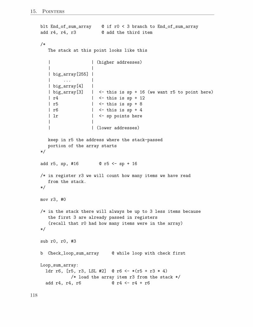
15. Pointers
blt End_of_sum_array @ if r0 < 3 branch to End_of_sum_array
add r4, r4, r3 @ add the third item
/*
The stack at this point looks like this
| | (higher addresses)
| |
| big_array[255] |
| ... |
| big_array[4] |
| big_array[3] | <- this is sp + 16 (we want r5 to point here)
| r4 | <- this is sp + 12
| r5 | <- this is sp + 8
| r6 | <- this is sp + 4
| lr | <- sp points here
| |
| | (lower addresses)
keep in r5 the address where the stack-passed
portion of the array starts
*/
add r5, sp, #16 @ r5 <- sp + 16
/* in register r3 we will count how many items we have read
from the stack.
*/
mov r3, #0
/* in the stack there will always be up to 3 less items because
the first 3 are already passed in registers
(recall that r0 had how many items were in the array)
*/
sub r0, r0, #3
b Check_loop_sum_array @ while loop with check first
Loop_sum_array:
ldr r6, [r5, r3, LSL #2] @ r6 <- *(r5 + r3 * 4)
/* load the array item r3 from the stack */
add r4, r4, r6 @ r4 <- r4 + r6
118

15.4. Passing a big array by value
/* accumulate in r4 */
add r3, r3, #1 @ r3 <- r3 + 1
/* move to the next item */
Check_loop_sum_array:
cmp r3, r0 @ r0 - r3 and update cpsr */
blt Loop_sum_array @ if r3 < r0 branch to Loop_sum_array */
End_of_sum_array:
mov r0, r4 @ r0 <- r4, to return the value of the sum */
pop {r4, r5, r6, lr}
bx lr
The function is not particularly complex except for the special handling of the first 3items (stored in r1 to r3) and that we have to be careful when locating elements ofthe array inside the stack. Upon entering the function the items of the array passedthrough the stack are laid out consecutively starting from sp. The push instruction atthe beginning pushes onto the stack four registers (r4, r5, r6 and lr) so our arrayis now in sp + 16 (see the diagram) and is eight byte aligned. Beside these details, wejust loop through the items of the array and accumulate the sum in register r4. Finally,we move r4 into r0 for the return value of the function.
In order to call this function we have to put an array into the stack. Consider thefollowing program.
.data
big_array:
.word 0, 1, 2, 3, 4, 5, 6, 7, 8, 9, 10, 11, 12, 13, 14, 15, 16, 17, 18
.word 19, 20, 21, 22, 23, 24, 25, 26, 27, 28, 29, 30, 31, 32, 33, 34, 35
.word 36, 37, 38, 39, 40, 41, 42, 43, 44, 45, 46, 47, 48, 49, 50, 51, 52
.word 53, 54, 55, 56, 57, 58, 59, 60, 61, 62, 63, 64, 65, 66, 67, 68, 69
.word 70, 71, 72, 73, 74, 75, 76, 77, 78, 79, 80, 81, 82, 83, 84, 85, 86
.word 87, 88, 89, 90, 91, 92, 93, 94, 95, 96, 97, 98, 99, 100, 101, 102
.word 103, 104, 105, 106, 107, 108, 109, 110, 111, 112, 113, 114, 115
.word 116, 117, 118, 119, 120, 121, 122, 123, 124, 125, 126, 127
message: .asciz "The sum of 0 to 127 is %d\n"
.text
.globl main
sum_array_value :
/* code shown above */
119

15. Pointers
main:
push {r4, r5, r6, r7, r8, lr}
/* we will not use r8 but we need to keep the function 8-byte aligned */
ldr r4, =big_array
/* Prepare call */
mov r0, #128 @ r0 <- 128
/* Load in the 1st parameter the number of items */
ldr r1, [r4] @ load in the 2nd parameter the 1st array item
ldr r2, [r4, #4] @ load in the 3rd parameter the 2nd array item
ldr r3, [r4, #8] @ load in the 4th parameter the 3rd array item
/* before pushing anything in the stack keep its position */
mov r7, sp
/* We cannot use more registers, now we have to push them
onto the stack (in reverse order) */
mov r5, #127 @ r5 <- 127
/* This is the last item position
(note that the first would be in position 0) */
b Check_pass_parameter_loop @ while loop testing first
Pass_parameter_loop:
ldr r6, [r4, r5, LSL #2] @ r6 <- *(r4 + r5 * 4).
/* loads the item in position r5 into r6.
Note that we have to multiply by 4 because that is
the size of each item in the array */
push {r6} @ push the loaded value to the stack */
sub r5, r5, #1
/* we are done with the current item,
go to the previous index of the array */
Check_pass_parameter_loop:
cmp r5, #2 @ compute r5 - #2 and update cpsr
bne Pass_parameter_loop @ if r5 != #2 => Pass_parameter_loop
/* We are done, we have passed all the values of the array,
now call the function */
bl sum_array_value @ Finally we call the function
120

15.5. Passing a big array by reference
/* restore the stack position */
mov sp, r7
/* prepare the call to printf */
mov r1, r0 /* second parameter, the sum itself */
ldr r0, =message /* first parameter, the message */
bl printf
pop {r4, r5, r6, r7, r8, lr}
bx lr
We start by preparing the call to sum array value. The first parameter, passed inregister r0, is the number of items of this array (in the example hardcoded to 128items). Then we pass the first three items of the array (if there are that many) inregisters r1 to r3. Any remaining items must be passed on the stack. Remember thatin a stack the last item pushed will be the first popped, so if we want our array be laidin the same order we have to push it in backwards. So we start from the last item, themov r5, #127, and then we load every item and push it onto the stack. Once all theelements have been pushed onto the stack we can finally call sum array value.
A very important caveat when manipulating the stack in this way is that it is critical torestore it and leave it in the same state as it was before preparing the call. This is thereason we keep sp in r7 before pushing anything onto the stack and we restore it rightafter the call to sum array values. Forgetting to do this will make further operationson the stack push data onto the wrong place or pop the wrong data from the stack.Keeping the stack synchronized is essential when calling functions.
15.5 Passing a big array by reference
Now you are probably thinking that passing a big array through the stack (along withall the boilerplate that this requires) to a function that does not modify it, is, to saythe least, wasteful.
Note that, when the amount of data is small, registers r0 to r3 are usually enough, sopass by value is affordable. Passing some data in the stack is fine too, but passing bigstructures on the stack may harm the performance (especially if our function is beingcalled lots of times).
Can we do better? Yes. Instead of passing copies of the values of the array, would it bepossible to pass the address of the array? The answer is, again, yes. This is the conceptof pass by reference. When we pass by value, the value of the data passed is somehowcopied (either in a register or a stack). Here we will pass a reference (i.e., an address)to the data. So now all we need do is just pass the number of items and then the address
121

15. Pointers
of the array, and let the function use this address to perform its computation.
Consider the following program, which also sums an array of integers but now passingthe array by reference.
.data
big_array:
/* Same as above */
message: .asciz "The sum of 0 to 255 is %d\n"
.text
.globl main
sum_array_ref: /* We have passed all the data by reference */
/* Parameters:
r0 = Number of items
r1 = Address of the array
*/
push {r4, r5, r6, lr}
mov r4, #0 @ r4 <- 0 @ the sum so far
mov r5, #0 @ r5 <- 0 @ number of items processed
b Check_loop_array_sum @ while loop, check first
Loop_array_sum:
ldr r6, [r1, r5, LSL #2] @ r6 <- *(r1 + r5 * 4)
add r4, r4, r6 @ r4 <- r4 + r6
add r5, r5, #1 @ r5 <- r5 + 1
Check_loop_array_sum:
cmp r5, r0 @ r5 - r0 and update cpsr
bne Loop_array_sum @ if r5 != r0 go to Loop_array_sum
mov r0, r4 @ r0 <- r4, to return the value of the sum
pop {r4, r5, r6, lr}
bx lr
main:
push {r4, lr}
/* we will not use r4 but we need to keep the stack 8-byte aligned */
122

15.6. Modifying data through pointers
mov r0, #128
ldr r1, =big_array
bl sum_array_ref
/* prepare the call to printf */
mov r1, r0 @ second parameter, the sum itself
ldr r0, =message @ first parameter, the message
bl printf
pop {r4, lr}
bx lr
Now the code is much simpler (and faster) as we avoid copying the values of the arrayin the stack. We simply pass the address of the array as the second parameter of thefunction and then we use it to access the array and compute the sum.
15.6 Modifying data through pointers
We saw at the beginning of this chapter that we could modify data through pointers.If we pass a pointer to a function we can let the function modify it as well. Imaginea function that takes an integer and increments it. We could do this by returning thevalue, for instance.
increment:
add r0, r0, #1 @ r0 <- r0 + 1
This takes the first parameter (in r0) increments it and returns it (recall that we returnintegers in r0).
An alternative approach, could be receiving a pointer to some data and let the functionincrement the data at the position defined by the pointer.
increment_ptr:
ldr r1, [r0] @ r1 <- *r0
add r1, r1, #1 @ r1 <- r1 + 1
str r1, [r0] @ *r0 <- r1
For a more elaborate example, let’s revisit the array code above but this time insteadof computing the sum of all the values, we will multiply each item by two and keep itin the same array. To prove that we have modified it, we will also print each item.
/* double_array.s */
.data
123

15. Pointers
big_array:
/* Same as above */
message: .asciz "Item at position %d has value %d\n"
.text
double_array:
/* Parameters:
r0 Number of items
r1 Address of the array
*/
push {r4, r5, r6, lr}
mov r4, #0 @ r4 <- 0
b Check_loop_array_double
Loop_array_double:
ldr r5, [r1, r4, LSL #2] @ r5 <- *(r1 + r4 * 4)
mov r5, r5, LSL #1 @ r5 <- r5 * 2 @ double
str r5, [r1, r4, LSL #2] @ *(r1 + r4 * 4) <- r5
add r4, r4, #1 @ r4 <- r4 + 1
Check_loop_array_double:
cmp r4, r0 @ r4 - r0 and update cpsr
bne Loop_array_double @ if r4 != r0 go to Loop_array_double
pop {r4, r5, r6, lr}
bx lr
print_each_item:
push {r4, r5, r6, r7, r8, lr} /* r8 is unused */
mov r4, #0 @ r4 <- 0
mov r6, r0 @ r6 <- r0. Keep r0 because we will overwrite it
mov r7, r1 @ r7 <- r1. Keep r1 because we will overwrite it
b Check_loop_print_items
Loop_print_items:
ldr r5, [r7, r4, LSL #2] @ r5 <- *(r7 + r4 * 4)
/* Prepare the call to printf */
ldr r0, =message @ 1st parameter of the call to printf
124

15.6. Modifying data through pointers
mov r1, r4 @ 2nd parameter: item position
mov r2, r5 @ 3rd parameter: item value
bl printf @ call printf
add r4, r4, #1 @ r4 <- r4 + 1
Check_loop_print_items:
cmp r4, r6 @ r4 - r6 and update cpsr
bne Loop_print_items @ if r4 != r6 goto Loop_print_items
pop {r4, r5, r6, r7, r8, lr}
bx lr
.globl main
main:
push {r4, lr}
/* we will not use r4 but we need to keep the stack 8-byte aligned */
/* first call print_each_item */
mov r0, #128 @ first_parameter: number of items
ldr r1, =big_array @ second parameter: address of the array
bl print_each_item @ call to print_each_item
/* call to double_array */
mov r0, #128 @ first_parameter: number of items
ldr r1, =big_array @ second parameter: address of the array
bl double_array @ call to double_array
/* second call print_each_item */
mov r0, #128 @ first_parameter: number of items
ldr r1, =big_array @ second parameter: address of the array
bl print_each_item @ call to print_each_item
pop {r4, lr}
bx lr
If you run this program you will see that the items of the array have been effectivelydoubled.
...
Item at position 123 has value 123
Item at position 124 has value 124
Item at position 125 has value 125
Item at position 126 has value 126
Item at position 127 has value 127
Item at position 0 has value 0
125

15. Pointers
Item at position 1 has value 2
Item at position 2 has value 4
Item at position 3 has value 6
Item at position 4 has value 8
...
15.7 Returning more than one piece of data
Functions, per the AAPCS convention, return their values in register r0 (and r1 if thereturned item is 8 bytes long). We can return more than one thing if we just pass apointer to some storage (possibly in the stack) as a parameter to the function. Someelementary practice with this idea appears in the Projects.
Projects
1. Modify the isort.s program to sort a file inplace passing the address of the fileas a parameter.
2. Write some programs that demonstrate returning more than one piece of datafrom a function.
3. Write some programs that demonstrate printing an array of floats.
126

16 System Calls
In Chapter 9 we saw the basics of how to call on Input/Output (I/O) functions availablethrough the C compiler. We used scanf(), printf(), puts() and, as C program-mers, we know there are many more such functions. They may, and should, be used byassembler programmers.
In embedded systems, however, we may find ourselves limited to using the assemblerand loader without the assistance of the C compiler. In the Projects in Chapter 1 wementioned how to perform the operations of assembling, linking/loading, and executingprograms directly. Looking back there we note another assembler operator: svc. Themneumonic stands for SerVice Call. Closely related is the operator swi standing forSoftWare Interrupt.
Although swi has been generally replaced by the equivalent svc, it still works andactually makes it easier to explain its function. The idea is that while the processor ofyour computer is running your program, it is (and must be) able to handle interruptionsby the hardware. For example, while computing your Fibonacci numbers, it must beable to react to a keystroke or a message from your printer. The system must carefullyinterrupt what it has been doing, handle the interruption (do whatever is necessary torespond), and then go back to doing your calculations.
We will look at these hardware interrupts later. Now we will consider the obvious otherkind of interrupt, the software interrupt. In that case, your program has in it codeto ask the processor to interrupt its usual flow of instructions and perform some codewritten into the Operating System (Raspbian for us).
There is a very long list of such code (functions) that are available and a search of theweb will let you find out what they all are. For us, only a few are of immediate interest.For example, the method of exiting a program was described in Chapter 1 and involves- as in all cases - storing in r7 the number of the service desired (#1 in the case ofexit) and then issuing the instruction svc 0.
In this chapter we will cover a few other services available, particularly those associatedwith file I/O functions. We will not use the C compiler in our examples.
127

16. System Calls
16.1 File I/O
Let’s look at the basic operations of opening a file, reading and/or writing from/to a file,and, finally, closing a file. The following program also uses our monitor and keyboard.
01 /* -- create.s -- */
02
03 .text
04 .global _start @ assemble, link/load, execute this code
05_start: @ see Chapter 1 Projects for instructions
06 push {r4, lr}
07
08 /* OPEN (CREATE) FILE */
09 ldr r0, =newfile
10 mov r1, #0x42 @ create R/W
11 mov r2, #384 @ = 600 octal (me)
12 mov r7, #5 @ open (create)
13 svc 0
14
15 cmp r0, #-1 @ file descriptor
16 beq err
17
18 mov r4, r0 @ save file_descriptor
19
20 /* PROMPT (WRITE) */
21 mov r0, #1 @ stdout (monitor)
22 ldr r1, =prompt @ address of prompt
23 mov r2, #(promptend - prompt) @ length of prompt
24 mov r7, #4 @ write
25 svc 0
26
27 /* READ */
28 mov r0, #0 @ stdin (keyboard)
29 ldr r1, =buffer @ address of buffer
30 mov r2, #26 @ maximum length of input
31 mov r7, #3 @ read
32 svc 0
33 mov r5, r0 @ save number of characters
34
35 /* WRITE TO FILE */
36 mov r0, r4 @ file_descriptor
37 ldr r1, =buffer @ address of buffer
38 mov r2, r5 @ length from read
39 mov r7, #4 @ write
128

16.1. File I/O
40 svc 0
41
42 /* CLOSE FILE */
43 mov r7, #6 @ close
44 svc 0
45 mov r0, r4 @ return file_descriptor as error code
46
47 exit: pop {r4, lr}
48 mov r7, #1 @ exit
49 svc 0
50
51 err: mov r4, r0
52 mov r0, #1
53 ldr r1, =errmsg
54 mov r2, #(errmsg - errmsgend)
55 mov r7, #4
56 svc 0
57
58 mov r0, r4
59 b exit
60
61 .data
62
63 errmsg: .asciz "create failed"
64 errmsgend:
65 newfile: .asciz "/home/pi/code/newfile"
66 prompt: .asciz "Input a string: \n"
67 promptend:
68 buffer: .byte 100
Here are descriptions of the operations performed in this sample program.
In lines 9-13 we create a new file. We use the OPEN operation which is service call #5placed in r7. The parameters for that call are as follows. r0 contains the address of astring with the fully qualified name of the desired file. r1 contains some flags (bits) todescribe what type of file it is to be. In hex they are concatenated together with 0 =read-only, 1 = write-only, and 2 = read and write. In addition, 0x40 = create if the filedoes not exist. Thus, we use 0x42 for a file which allows both reading and writing and,in addition, will be created if it does not exist.
Finally, in r2 we put some permission bits. The value we must insert is based on theRaspbian history of being a LINUX based system. File management in UNIX dividedusers up into three categories: owner, group, others. The permissions also includedthree classes: Read, Write, and eXecute. The command ls -la gives a listing of filesand shows on the left their permissions in the form of a string such as rwxrwxrwx. It
129

16. System Calls
is preceded by a “d” if it is a directory, while a “-” indicates the premission is lacking.Looking at that string as a nine bit binary number, we can set permissions for the threeclasses going left to right. In our example we used 600OCT to indicate read and writepermissions for the user (me) [note that 700 would have allowed execution also]. Wegave no permissions to the group or others (but could have).
This OPEN operation returns (in r0 of course) a number which is called the file de-scriptor. It is by that number that one refers to the file in the future. If there is anerror while trying to OPEN the file, it returns -1 so the user can handle the problem.
The WRITE operation in lines 21-25 uses the service call #4 in r7. The parameters are:In r0 is the file descriptor #1 which is always the stdout ; i.e., the monitor. In r1 we putaddress of the string we want to display. Finally, in r2 we put how many characters wewant to write. In our case we let the assembler calculate how many characters thereare in our prompt (it can do that!) since we might change the prompt later and thecalculation method avoids human error in counting again.
The READ in lines 28-33 uses the service call #3 in r7. The parameters are similar tothe WRITE operation. In r0 we place the file descriptor #0 which is always the stdin;i.e., the keyboard. In r1 we put the address of where we want to place the input string.Finally, in r2 we put how many characters (at most) we want to read. Note that in line68 we made room for 100 bytes (just in case) and then only asked for 26 characters online 30 (for no particular reason).
The READ operation returns the number of characters actually read (before the carriagereturn) and we saved that number in r5 on line 33. Since we had room in buffer, wemight have allowed it to try to read more characters.
The interesting WRITE TO FILE operation on lines 36-40 shows how easy it is toperform the task. Since it is a WRITE we again use service call #4. As before r0
contains the file descriptor but this time it is the one returned by the OPEN (CREATE)and saved in r4. r1 gets the address of the buffer where the string to be written is.r2 gets the number of characters we want to write that we saved in r5.
When programming in a high-level language such as C or Python, users often expectand use the fact that when their program terminates all the files they used are carefullysaved by the operating system. For assembler language programmers we might be moreaware of how systems actually operate and be wary of any assumptions. It is possiblethat when we think we are writing to a file we are actually only writing the informationinto a buffer maintained by the operating system so that it can optimize its accesses tothe file by waiting for additional data.
While it’s usually not necessary, for good programming practice we should CLOSEthe file when we are done with it, thus telling the system to make sure all data hasbeen saved. It’s very simple. As on lines 43-45, we merely use service call #6 with r0
containing the file descriptor for the file (here we assume it’s still there from line 36).
130

16.2. lseek
Obviously we have included some code to handle a case where the OPEN (CREATE)operation did not succeed.
16.2 lseek
The system calls we have described in detail can be given in C notation as follows:
int open ( char* full_path_name , int flags , int permissions );
int write ( int file_descriptor , char* buffer , int length );
int read ( int file_descriptor , char* buffer , int length );
void close ( int file_descriptor );
Another very valuable call useful when reading and writing files is lseek. It allows us tomove to a particular spot in a file. Without it, we might have to start at the beginningof every file and then read through the file until reaching the data we want and then westill might not be able to change the data without further complications.
The form of this call in C is
int lseek ( int file_descriptor , int offset , int mode );
The file descriptor is, of course, the one we used before associated with the file. Thevalues of mode can be 0, 1, or 2. The offset is the number of bytes to move dependingon the mode. If the mode is 0, then the offset is from the beginning of the file. If modeis 1, then the offset is from the present position in the file. Finally, if mode is 2, theoffset is relative to the end of the file.
The system call associated with this C function is #19. The parameters can be figuredout by looking at the above functions and the C prototype.
Note that this function allows us to go directly to the end of a file and append additionaldata when we open the file by concatenating 0x400 to the flags on line 10 of our create.scode.
Projects
1. Modify the isort.s program to sort a file whose name is input by the user.
2. Write some programs that demonstrate reading and printing an array of floatsthat are in a file.
3. There are many other system calls available such as getting the time (#13) or mak-ing a directory (mkdir = #39). Look up such calls and note how the parametersusually follow those of the associated C code.
131

16. System Calls
4. Try some file manipulations that use lseek that has system call number #19.
5. In the create.s program, test to see what happens if the file already exists. Howmany characters are actually written into the file?
132

17 Local data
Most of our examples involving data stored in memory (in contrast to data stored inregisters) have used global variables. Global variables are global names, i.e., addressesof the memory that we use through labels. These addresses, somehow, pre-exist beforethe program runs. This is because we define them when defining the program itself.
Sometimes, though, we may want data stored in memory the existence of which is nottied to the program existence but to the dynamic activation of a function. You mayrecall from previous chapters, that the stack allows us to store data the lifetime of whichis the same as the dynamic activation of a function. This is where we will store localvariables, which in contrast to global variables, only exist because the function theybelong has been dynamically activated (i.e. called/invoked).
In Chapter 15 we passed a very big array through the stack in order to pass the arrayby value. This will lead us to the conclusion that, somehow, parameters act as localdata, in particular when they are passed through the stack.
17.1 The frame pointer
In the ARM processor, we have plenty of general-purpose registers (up to 16, albeitsome of them with very narrow semantics, so actually about 12 are actually useable asgeneral-purpose) and the AAPCS forces us to use registers for the first four parameters(r0 to r3). Note how this is consistent with the fact that these four registers are caller-saved while all other registers are callee-saved. Other architectures, like the 386, havea lower number of general purpose registers (about 6) and the usual approach whenpassing data to functions always involves the stack. This is so because with such asmall number of registers, passing parameters through registers, would force the callerto save them, usually in the stack or some other memory, which in turn will usuallyrequire at least another register for indexing! By using the stack a few more registersare easily available.
Up to this point one might wonder why we don’t always pass everything through thestack and forget about registers r0 to r3. Well, passing through registers is going to befaster as we do not have to mess with loads and stores from or to the memory whichis much slower than register accesses. In addition, most functions receive just a few
133

17. Local data
parameters, or at least not many more than four, so it makes sense to exploit thisfeature.
But then a problem arises, what if we are passing parameters through the stack and atthe same time we have local variables. Both entities will be stored in the stack. Howcan we deal with the two sources of data which happen to be stored in the same memoryarea?
Here is where the concept of frame pointer appears. A frame pointer is a sort of markerin the stack that we will use to tell apart local variables from parameters. We mustemphasize the fact that a frame register is almost always unnecessary and one canalways devise ways to avoid it. That said, a frame pointer gives us a consistent solutionto accessing local data and parameters in the stack. Of course, most good things comewith a price, and the frame pointer is not an exception: we need to use a register forit. Sometimes this restriction may be unacceptable so we can, almost always, get rid ofthe frame pointer.
Due to its optional nature, the frame pointer is not specified nor mandated by theAAPCS. That said, the usual approach is using register r11. As an extension (appar-ently undocumented, as far as we have been able to tell) we can use the name fp whichis far more informative than just r11. Nothing enforces this choice, we can use anyother register as frame pointer. Since we will use fp (i.e., r11) we will have to refrainfrom using r11 for any other purpose.
17.2 Dynamic link of the activation record
Activation record is a fancy name to specify the context of a called function. That is,the local data and parameters (if passed through the stack) of that function. Whena function is written using a frame pointer some bookkeeping is required to correctlymaintain the activation record.
First let’s examine the typical structure of a function.
function:
push {r4, lr} /* Keep the callee saved registers */
... /* code of the function */
pop {r4, lr} /* Restore the callee saved registers */
bx lr /* Return from the function */
Now let’s modify the function to use a frame pointer (in the code snippet below do notmind the r5 register that only appears here to keep the stack 8-byte aligned).
function:
push {r4, r5, fp, lr} /* Keep the callee saved registers.
We added r5 to keep the stack 8-byte aligned
134

17.2. Dynamic link of the activation record
but the important thing here is fp */
mov fp, sp /* fp <- sp. Keep dynamic link in fp */
... /* code of the function */
mov sp, fp /* sp <- fp. Restore dynamic link in fp */
pop {r4, r5, fp, lr} /* Restore the callee saved registers.
This will restore fp as well */
bx lr /* Return from the function */
Focus on the mov instructions just before and after the function code. We first keep theaddress of the top of the stack in fp. After the function call we restore the value ofthe stack using the value kept in fp. Now you should see why we said that the framepointer is usually unnecessary: if the sp register does not change between those moves,having a frame pointer will be pointless, why should we restore a register that didn’tchange?
Let’s assume for now that the frame pointer is going to be useful. What we did in thefirst mov instruction was setting the dynamic link. The stack and registers will look likethis after we have set it.
Figure 17-1
As you can see, the fp register will point to the top of the stack. But note that in thestack we have the value of the old fp (the value of the fp in the function that calledus). If we assume that our caller also uses a frame pointer, then the fp we kept in thestack of the callee points to the top of the stack when our caller was called.
But still this looks useless because both registers fp and sp in the current function pointto the same position in the stack.
Let’s proceed with the example and be sure to check the sub command where we enlargethe stack.
135

17. Local data
function:
/* Keep callee-saved registers */
push {r4, r5, fp, lr} /* Keep the callee saved registers.
We added r5 to keep the stack 8-byte aligned
but the important thing here is fp */
mov fp, sp /* fp <- sp. Keep dynamic link in fp */
sub sp, sp, #8 /* Enlarge the stack by 8 bytes */
... /* code of the function */
mov sp, fp /* sp <- fp. Restore the dynamic link in fp */
pop {r4, r5, fp, lr} /* Restore the callee saved registers.
This will restore fp as well */
bx lr /* Return from the function */
Now, after enlarging the stack, the stack and registers will look like this.
Figure 17-2
Can you see the range of data from sp to fp? This is the local data of our function.We will keep local variables of a function in this space when using a frame pointer. Wesimply have to allocate stack space by decreasing the value of sp (and ensuring it is8-byte aligned per AAPCS requirements).
Now consider the instruction mov sp, fp near the end of the function. What it doesis leaving the state of the registers just like before we enlarged the stack (before thesub sp, sp, #8). And voila, we have freed all the area of the stack that our functionwas using. A bonus of this approach is that it does not require keeping anywhere thenumber of bytes we reserved on the stack. Neat, isn’t it?
136

17.3. What about parameters passed in the stack?
17.3 What about parameters passed in the stack?
A player is still missing in our frame pointer approach: parameters passed through thestack. Let’s assume that our function may receive parameters in the stack and we haveenlarged the stack by subtracting from sp. The whole picture looks like this.
Figure 17-3
Notice that we lied a bit in the two first figures. In them, the old fp pointer kept inthe stack pointed to the top of the stack of the caller. Not exactly, it will point to thebase of the local data of the caller, exactly like what happens with the fp register inthe current function.
17.4 Indexing through the frame pointer
When we are using a frame pointer a nice property (that maybe you have alreadydeduced from the figures above) holds: local data is always at lower addresses than theaddress pointed by fp while parameters passed in the stack (if any) will always be athigher addresses than the one pointed by fp. It must be possible to access both kindsof local data through fp.
In the following example we will use a function that receives an integer by reference(i.e., an address to an integer) and then squares that integer. In C that is:
void sq(int *c)
{
(*c) = (*c) * (*c);
}
137

17. Local data
You may be wondering why the function sq has a reference parameter (should it not beeasier to return a value?), but bear with us for now. We can (should?) implement sq
without using a frame pointer due to its simplicity.
sq:
ldr r2, [r0] @ r2 <- (*r0)
ldr r3, [r0] @ r3 <- (*r0)
mul r1, r2, r3 @ r1 <- r2 * r3
str r1, [r0] @ (*r0) <- r1
bx lr @ Return from the function
Now consider the following function that returns the sum of the squares of its fiveparameters. It uses the function sq defined above.
int sq_sum5(int a, int b, int c, int d, int e)
{
sq(&a);
sq(&b);
sq(&c);
sq(&d);
sq(&e);
return a + b + c + d + e;
}
Parameters a, b, c and d will be passed through registers r0, r1, r2, and r3 respec-tively. The parameter e will be passed through the stack. The function sq, though,expects a reference, i.e., an address, to an integer and registers do not have an address.This means we will have to allocate temporary local storage for these registers. At leastone integer will have to be allocated in the stack in order to be able to call sq but forsimplicity we will allocate four of them.
This time we will use a frame pointer to access both the local storage and the parametere.
sq_sum5:
push {fp, lr} /* Keep fp and all callee-saved registers. */
mov fp, sp /* Set the dynamic link */
sub sp, sp, #16 /* Allocate space for 4 integers in the stack */
/* Keep parameters in the stack */
str r0, [fp, #-16] @ *(fp - 16) <- r0
str r1, [fp, #-12] @ *(fp - 12) <- r1
str r2, [fp, #-8] @ *(fp - 8) <- r2
str r3, [fp, #-4] @ *(fp - 4) <- r3
138

17.4. Indexing through the frame pointer
/* At this point the stack looks like this
| Value | Address(es)
+--------+-----------------------
| r0 | [fp, #-16], [sp]
| r1 | [fp, #-12], [sp, #4]
| r2 | [fp, #-8], [sp, #8]
| r3 | [fp, #-4], [sp, #12]
| fp | [fp], [sp, #16]
| lr | [fp, #4], [sp, #20]
| e | [fp, #8], [sp, #24]
v
Higher
addresses
*/
sub r0, fp, #16 @ r0 <- fp - 16
bl sq @ call sq(&a);
sub r0, fp, #12 @ r0 <- fp - 12
bl sq @ call sq(&b);
sub r0, fp, #8 @ r0 <- fp - 8
bl sq @ call sq(&c);
sub r0, fp, #4 @ r0 <- fp - 4
bl sq @ call sq(&d)
add r0, fp, #8 @ r0 <- fp + 8
bl sq @ call sq(&e)
ldr r0, [fp, #-16] @ r0 <- *(fp - 16). Loads a into r0
ldr r1, [fp, #-12] @ r1 <- *(fp - 12). Loads b into r1
add r0, r0, r1 @ r0 <- r0 + r1
ldr r1, [fp, #-8] @ r1 <- *(fp - 8). Loads c into r1
add r0, r0, r1 @ r0 <- r0 + r1
ldr r1, [fp, #-4] @ r1 <- *(fp - 4). Loads d into r1
add r0, r0, r1 @ r0 <- r0 + r1
ldr r1, [fp, #8] @ r1 <- *(fp + 8). Loads e into r1
add r0, r0, r1 @ r0 <- r0 + r1
mov sp, fp /* Undo the dynamic link */
pop {fp, lr} /* Restore fp and callee-saved registers */
bx lr /* Return from the function */
As you can see, we first store all parameters (but e) in the local storage. That meansthat we need to enlarge the stack enough, as usual, by subtracting from sp. Once wehave the storage then we can do the actual store by using the fp register. Note the
139
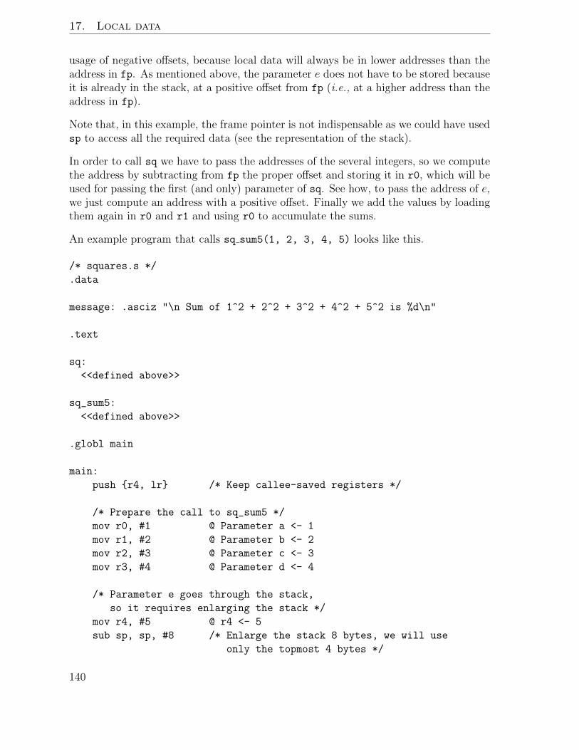
17. Local data
usage of negative offsets, because local data will always be in lower addresses than theaddress in fp. As mentioned above, the parameter e does not have to be stored becauseit is already in the stack, at a positive offset from fp (i.e., at a higher address than theaddress in fp).
Note that, in this example, the frame pointer is not indispensable as we could have usedsp to access all the required data (see the representation of the stack).
In order to call sq we have to pass the addresses of the several integers, so we computethe address by subtracting from fp the proper offset and storing it in r0, which will beused for passing the first (and only) parameter of sq. See how, to pass the address of e,we just compute an address with a positive offset. Finally we add the values by loadingthem again in r0 and r1 and using r0 to accumulate the sums.
An example program that calls sq sum5(1, 2, 3, 4, 5) looks like this.
/* squares.s */
.data
message: .asciz "\n Sum of 1^2 + 2^2 + 3^2 + 4^2 + 5^2 is %d\n"
.text
sq:
<<defined above>>
sq_sum5:
<<defined above>>
.globl main
main:
push {r4, lr} /* Keep callee-saved registers */
/* Prepare the call to sq_sum5 */
mov r0, #1 @ Parameter a <- 1
mov r1, #2 @ Parameter b <- 2
mov r2, #3 @ Parameter c <- 3
mov r3, #4 @ Parameter d <- 4
/* Parameter e goes through the stack,
so it requires enlarging the stack */
mov r4, #5 @ r4 <- 5
sub sp, sp, #8 /* Enlarge the stack 8 bytes, we will use
only the topmost 4 bytes */
140

17.4. Indexing through the frame pointer
str r4, [sp] @ Parameter e <- 5
bl sq_sum5 @ call sq_sum5(1, 2, 3, 4, 5)
add sp, sp, #8 @ Shrink back the stack
/* Prepare the call to printf */
mov r1, r0 @ The result of sq_sum5
ldr r0, =message
bl printf @ Call printf
pop {r4, lr} /* Restore callee-saved registers */
bx lr
$ ./squares
Sum of 1ˆ 2 + 2ˆ 2 + 3ˆ 2 + 4ˆ 2 + 5ˆ 2 is 55
Projects
1. Rewrite some earlier programs to pass the parameters by reference.
2. Rewrite some earlier programs to reference variables using the frame pointer,even if it is not necessary.
141


18 Inline Assembler in C Code
Although we have concentrated on Assembler programming, we must admit that almostevery microprocessor system comes with an excellent C compiler and it is expected thatprogrammers will write in C. Sometimes, however, it is necessary to optimize the codeby manually inserting assembler code into the C source code. Based on the GNUC compiler, most manufacturers allow for inline assembler code. Unfortunately, eachcompany does it slightly differently so one must learn the details of each system thatone uses.
18.1 The asm Statement
The format of the new asm statement is as follows:
asm("<list of assembler instructions>"
: <list of write-only parameter formats and names>
: <list of read-only parameter formats and names>
: <list of registers that are changed (clobbered) by the code>
);
The details of using this instruction are many and complicated. Some requirements areunfortunate but depended on the whim of the compiler writer.
If there are no registers that are modified, the third colon “:” is not necessary. If thereare no write-only parameters but some read-only ones, they must be preceded by twocolons. The following is an example where there are no parameters at all:
int return1(void) {asm("mov r0, #1");}
This trivial function returns the integer value 1 in the usual register r0. No colons arenecessary. It is not necessary to inform the compiler that r0 is being changed.
Another simple example is the following complete C program that initializes two globalvariables “i” and “j ” and takes no parameters and returns nothing. The output shouldbe “i = 100 and j = 200” after running the program.
int i, j;
143

18. Inline Assembler in C Code
void Initialization(void)
{
asm("mov r0, #0; add %0, r0, #100 ; add %1, r0, #200" : "+r" (i), "+r" (j));
}
void main(void)
{
Initalization();
printf("\n i = %d and j = %d \n", i , j);
}
Since there is just one colon before the parameter formats and names, they are write-only. Because of the ordering of the list, variable “i” is referenced by “%0” and variable“j” by “%1”. This count may be continued for additional parameters. [This is an oldermethod that still works. A more recent way to refer to names is given below.] Theformats are both “+r” (the strings themselves) in this case (the “+r” means it is read-write). The choices include “=r” for a write-only parameter with an integer registerassociated with it, and “=f” for a write-only parameter with a floating point registerassociated. By the way, they may be either global or local variables in general. We alsonote that the number of colons and the prefix “=” are redundant but that’s how to doit.
The style of programming we will use here will be to write the I/O portion of the programin C and do most of the actual processing in called functions written in assembler. Thisfollows the HIPO (Hierarchical Input Process Output) model nicely.
18.2 Simple Example
We have said that multiplication is much slower than such operations as addition orshifting. If we wish to multiply a number by three, we might improve our performanceby using the trick shown earlier.
#include <stdio.h>
int triple(int n)
{
asm("add %[value], %[value], %[value], LSL #1" : [value] "+r" (n));
}
int main(void)
{
int n;
printf("\nTriple Program!\n");
printf("\nEnter an integer: ");
144
18.2. Simple Example
scanf(%d, &n);
printf("\nThree times %d is %d", n, triple(n));
}
In this code section we refer to the operands by the percent sign (%) followed bya symbolic name in square brackets. These names are independent of names usedelsewhere in the program.
Of course a very intelligent C compiler might optimize the code for us but this issupposed to be a trivial example. The general idea is that in many large programs, onlya very small amount of the code takes up most of the processing time. Optimizing thatpart can give big savings.
We will not go into great detail concerning inline code since good C compilers areavailable and good references, such as those given in the Projects, are also available.
Projects
1. Rewrite some earlier programs using some inline assembler code.
2. Look up more detailed information concerning inline assembler using the GCCcompiler at locations such as:
a) https://www.fdi.ucm.es/profesor/mendias/PSyD/docs/ARM GCC Inline As-sembler Cookbook.pdf
b) http://www.ethernut.de/en/documents/arm-inline-asm.html.
145


19 Thumb
Several times in previous chapters we have talked about ARM as an architecture thathas several features aimed at embedded systems. In such systems memory is scarce andexpensive, so designs that help reduce the memory footprint are very welcome. Here wewill see another of these features: the Thumb instruction set.
19.1 The Thumb instruction set
In earlier chapters we have been working with the ARMv6 instruction set (the oneimplemented in the Raspberry Pi). In this instruction set, all instructions are 32-bitswide, so every instruction takes 4 bytes. This is a common design since the arrival ofRISC processors. That said, in some scenarios such codification is overkill in terms ofmemory consumption: many platforms are very simple and rarely need all the featuresprovided by the instruction set. If only they could use a subset of the original instructionset that can be encoded in a smaller number of bits!
So, that is what the Thumb instruction set is all about. It is a reencoded subset ofthe ARM instructions that takes only 16 bits per instruction. That means that we willhave to do away with some instructions. As a benefit our code density is higher: mostof the time we will be able to encode the code of our programs in half the space.
19.2 Support of Thumb in Raspbian
While the processor of the Raspberry Pi properly supports Thumb, there is still somesoftware support that unfortunately is not provided by Raspbian. That means that wewill be able to write some snippets in Thumb but in general this is not supported (ifyou try to use Thumb for a full C program you will end with a sorry, unimplemented
message by the compiler).
19.3 Instructions
Thumb provides about 45 instructions (of about 115 in ARMv6). The narrower codi-fication of 16 bits means that we will be more limited in what we can do in our code.
147

19. Thumb
Registers are split into two sets: low registers, r0 to r7, and high registers, r7 to r15.Most instructions can only fully work with low registers and some others have limitedbehaviour when working with high registers.
Also, Thumb instructions cannot be predicated. Recall that almost every ARM instruc-tion can be made conditional depending on the flags in the cpsr register. That is notthe case in Thumb where only the branch instruction is conditional.
Mixing ARM and Thumb is only possible at the function level: a function must bewholly ARM or Thumb, it cannot be a mix of the two instruction sets. Recall thatour Raspbian system does not totally support Thumb so at some point we will have tojump from ARM code to Thumb code. This is done using the instruction (available inboth instruction sets) blx. This instruction behaves like the bl instruction we use forfunction calls but changes the state of the processor from ARM to Thumb (or Thumbto ARM).
We also have to tell the assembler that some portion of assembler is actually Thumbwhile the other is ARM. Since by default the assembler expects ARM, we will have tochange to Thumb at some point.
19.4 From ARM to Thumb
Let’s start with a very simple program returning an error code of 2 set in Thumb.
/* thumb-first.s */
.text
.code 16 /* Here we say we will use Thumb */
.align 2 /* Make sure instructions are aligned at 2-byte boundary */
thumb_function:
mov r0, #2 /* r0 <- 2 */
bx lr /* return */
.code 32 /* Here we say we will use ARM */
.align 4 /* Make sure instructions are aligned at 4-byte boundary */
.globl main
main:
push {r4, lr}
blx thumb_function /* From ARM to Thumb we use blx */
pop {r4, lr}
bx lr
Thumb instructions in our thumb function actually resemble ARM instructions. In fact
148

19.5. Calling functions in Thumb
most of the time there will not be much difference. As stated above, Thumb instructionsare more limited in features than their ARM counterparts.
If we run the program, it does what we expect.
$ ./thumb-first; echo $?
2
How can we tell our program actually mixes ARM and Thumb? We can use objdump
-d to dump the instructions of our thumb-first.o file.
$ objdump -d thumb-first.o
thumb-first.o: file format elf32-littlearm
Disassembly of section .text:
00000000 <thumb_function>:
0: 2002 movs r0, #2
2: 4770 bx lr
4: e1a00000 nop ; (mov r0, r0)
8: e1a00000 nop ; (mov r0, r0)
c: e1a00000 nop ; (mov r0, r0)
00000010 <main>:
10: e92d4010 push {r4, lr}
14: fafffff9 blx 0 <thumb_function>
18: e8bd4010 pop {r4, lr}
1c: e12fff1e bx lr
Check thumb function: its two instructions are encoded in just two bytes (instructionbx lr is at offset 2 from mov r0, #2). Compare this to the instructions in main: eachone is at offset 4 from its predecessor instruction. Note that some padding was addedby the assembler at the end of the thumb function in form of nops (that should not beexecuted, anyway).
19.5 Calling functions in Thumb
In Thumb we want to follow the AAPCS convention like we do when in ARM mode, butthen some oddities happen. Consider the following snippet where thumb function 1
calls thumb function 2.
.code 16 /* Here we say we will use Thumb */
.align 2 /* Make sure instructions are aligned at 2-byte boundary */
thumb_function_2:
149

19. Thumb
/* Do something here */
bx lr
thumb_function_1:
push {r4, lr}
bl thumb_function_2
pop {r4, lr} /* ERROR: cannot use lr in pop in Thumb mode */
bx lr
Unfortunately, this will be rejected by the assembler. If you recall from Chapter 11, inARM push and pop are mnemonics for stmdb sp! and ldmia sp!, respectively. But inThumb mode push and pop are instructions on their own and so they are more limited:push can only use low registers and lr, while pop can only use low registers and pc.The behaviour of these two instructions are almost the same as the ARM mnemonics.So, you are now probably wondering why these two special cases for lr and pc. This isthe trick: in Thumb mode pop {pc} is equivalent to pop the value val from the stackand then do bx val. So the two instruction sequence: pop {r4, lr} followed by bx
lr becomes simply pop {r4, pc}.
So, our code will look like this.
/* thumb-call.s */
.text
.code 16 /* Here we say we will use Thumb */
.align 2 /* Make sure instructions are aligned at 2-byte boundary */
thumb_function_2:
mov r0, #2
bx lr /* A leaf Thumb function (i.e. a function that does not call
any other function so it did not have to keep lr in the
stack) returns using "bx lr" */
thumb_function_1:
push {r4, lr}
bl thumb_function_2 /* From Thumb to Thumb we use bl */
pop {r4, pc} /* How we return from a non-leaf Thumb function */
.code 32 /* Here we say we will use ARM */
.align 4 /* Make sure instructions are aligned at 4-byte boundary */
.globl main
main:
push {r4, lr}
blx thumb_function_1 /* From ARM to Thumb we use blx */
150

19.6. From Thumb to ARM
pop {r4, lr}
bx lr
19.6 From Thumb to ARM
Finally we may want to call an ARM function from Thumb. As long as we stick toAAPCS everything should work correctly. The Thumb instruction to call an ARMfunction is again blx. Following is an example of a small program that says “Helloworld” four times calling printf, a function in the C library that in Raspbian is ofcourse implemented using ARM instructions.
/* thumb-first.s */
.data
message: .asciz "Hello world %d\n"
.text
.code 16 /* Here we say we will use Thumb */
.align 2 /* Make sure instructions are aligned at 2-byte boundary */
thumb_function:
push {r4, lr} /* keep r4 and lr in the stack */
mov r4, #0 /* r4 <- 0 */
b check_loop /* unconditional branch to check_loop */
loop:
/* prepare the call to printf */
ldr r0, =message /* r0 <- &message */
mov r1, r4 /* r1 <- r4 */
blx printf /* From Thumb to ARM we use blx.
printf is a function in the C library that is
implemented using ARM instructions */
add r4, r4, #1 /* r4 <- r4 + 1 */
check_loop:
cmp r4, #4 /* compute r4 - 4 and update the cpsr */
blt loop /* if r4 < 4 then branch to loop */
pop {r4, pc} /* restore registers and return from Thumb function */
.code 32 /* Here we say we will use ARM */
.align 4 /* Make sure instructions are aligned at 4-byte boundary */
.globl main
main:
push {r4, lr} /* keep r4 and lr in the stack */
151

19. Thumb
blx thumb_function /* from ARM to Thumb we use blx */
pop {r4, lr} /* restore registers */
bx lr /* return */
19.7 To know more
You may want to check the Thumb 16-bit Instruction Set Quick Reference Card providedby ARM:
http://infocenter.arm.com/help/topic/com.arm.doc.qrc0006e/QRC0006_UAL16.pdf
When checking that card, be aware that the processor of the Raspberry Pi only imple-ments ARMv6T, not ARMv6T2.
Finally, even more information is available from ARM in its “ARM Architecture Refer-ence Manual” (copies are available at many sites on-line).
Projects
1. Rewrite some earlier programs using Thumb code.
2. Look up more detailed information concerning Thumb code using the GCC com-piler.
152

20 Additional Topics
If the reader has covered most of the preceding chapters, he or she should be preparedto practice another important ability: to be able to read and understand the manualsconcerning the hardware and software they wish to use. For our purposes, the “ARMArchitecture Reference Manual” (often called the “ARM ARM”) mentioned in the lastchapter is important. It may be down-loaded from the web but, since it is 642 pages,probably not printed out.
20.1 ARM Instruction Set
In Part A we find described the CPU Architecture. More information is given formany of the topics we have already covered. In Chapter A3, however, is detailed materialon the ARM Instruction Set. This subject is very important for engineers interestedin the hardware of a computer.
ARM Instruction Set
Although some explanations of the letters that appear in the table are needed, this gives
153

20. Additional Topics
us an idea of the complexity of designing the instruction set of a computer. Detailsof the actual instruction encoding appears in the rest of that chapter of the “‘ARMARM”. Since the chapter is 42 pages long, we will let the reader use the manual to gaininformation about those details. Note that Chapter A4 gives a total of 290 pages ofdetails for each of the instructions!
20.2 Interrupt Handling
Another critical topic concerning computer architecture is how the system handles In-terrupts, also called Exceptions. Programmers should be aware that the operatingsystem is being interrupted constantly by (at least) the system clock. In addition, everyperipheral device must check in with the operating system regularly. Finally, as we sawpreviously, the operating system must handle our SerVice Calls (svc) or, equivalently,SoftWare Interrupts (swi).
We have mentioned the Current Program Status Register (cpsr) before. Its format,from A2-11 of the “ARM ARM” is:
CPSR
and the meanings of the fields are described there.
The four bits 31-28 are those associated with the condition codes we have used before.Bits 4-0 give the mode of operation.
Mode bits
There are seven modes in which the system may be running as shown above. All themodes other than User are privileged ; that is, they are able to use all the system’sresources. In order to handle exceptions quickly, the processor has more registers thanwe have admitted before. In particular, each of the first five privileged modes (that is,not including the System mode) has a separate spsr (Saved Program Status Register)in which the cpsr of the process that was running when the exception arose is stored.In addition they also have their own r13 and r14 registers so that they will not corrupt
154

20.3. To know more
those of the user’s process while they run. In addition, in order to make the FastInterrupt not have to save registers, that mode has its own r8 through r12 registers.See Figure A2-1 Register organization from the “ARM ARM”:
Register Organization
Clearly, the designers of the ARM processor gave great attention to the problem of howto handle interrupts quickly.
20.3 To know more
Read the entire “ARM ARM”! Of course that’s more than one wants to know aboutthe processor but scanning the manual to see what’s available is reasonable.
For advanced information about such topics as pipelining and cache handling, see thetext by Patterson and Hennessy, Computer Organization and Design, (ARM Edition),Morgan Kaufmann (Elsevier), 2017.
Projects
1. If you have taken an Operating Systems course, consider how the ARM allows foruninterruptable operations leading to having semaphores.
155

20. Additional Topics
2. Look up more detailed information concerning Java code using the Jazelle stateof the processor.
156
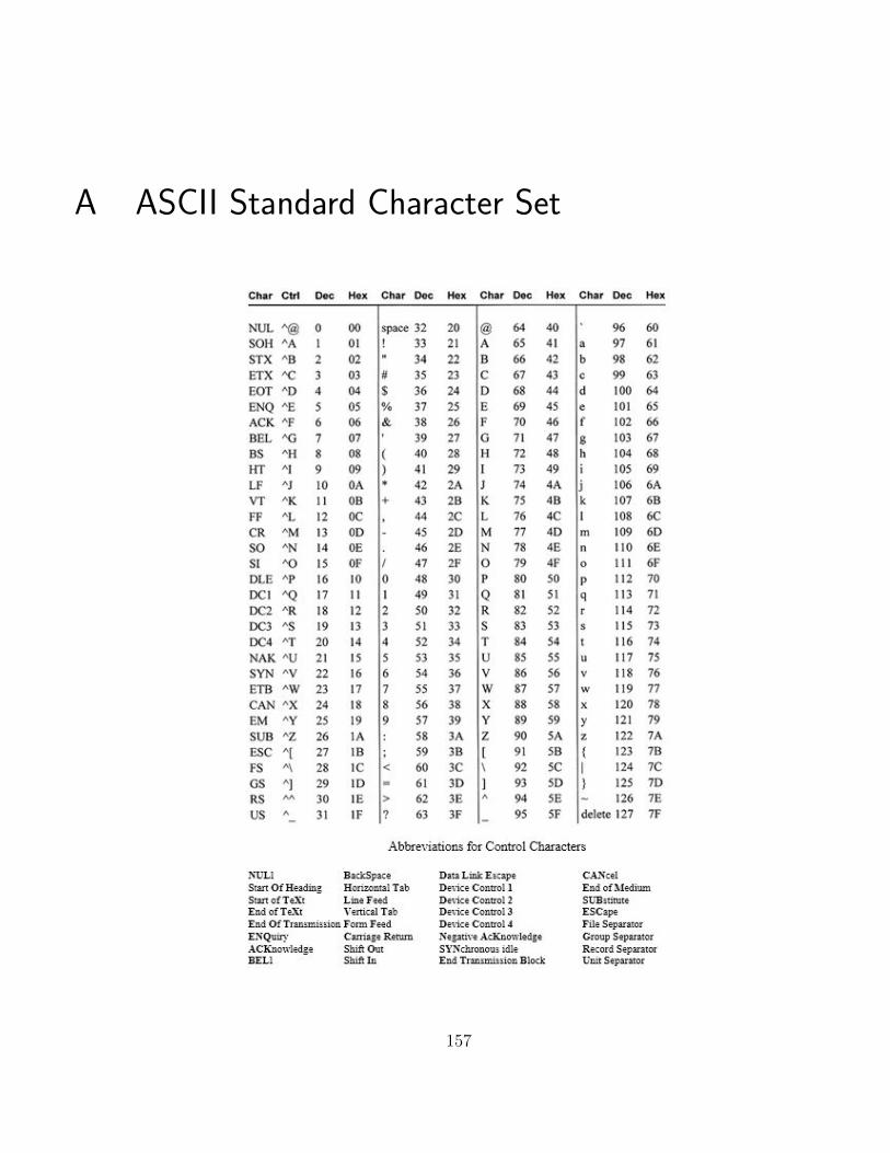
A ASCII Standard Character Set
157


B Integers
For scientists and engineers, computers are used to do arithmetic computations. In thischapter we will discuss the basics of how integer numbers are stored and manipulated.Later we will see that real numbers are stored quite differently.
B.1 Unsigned Integers
We may give an interpretation of bit patterns in an eight-bit byte as the integers from0x00 = 0DEC to 0xFF = 255DEC = 28–1. The ARM processor that we study in ChapterOne has registers in which one can store integers that are 32 bits in size so we willusually work with these longer groupings. It is easy to see that these four byte (32bit) configurations may be taken to represent all the unsigned integers from 0DEC =0x00000000 to 232–1 = 4, 294, 967, 295DEC = 0xFFFFFFFF.
Of course we do not want to be limited to non-negative integers so the interestingquestion is how to represent negative numbers using some of the 232 patterns available.In the next sections we will look at two simple ways that are rarely used and thenthe actual standard system (2’s complement). Still another system will be treated inChapter 13 since it is part of the standard method used for representing real numbers(IEEE-754).
B.2 Signed-Magnitude Integers
Before considering one of the many ways to represent integers so as to allow for bothpositive and negative numbers we will agree on a numbering scheme for the bits. It doesnot matter which decision we make in terminology but it may be convenient to use zerofor the least significant bit. Thus in a 32-bit register we will call the right most or leastsignificant “bit 0” and count towards the left up to “bit 31” for the most significant.One advantage is that for the unsigned integers described above the nth bit is associatedwith the power 2n.
|31|30292827262524232221201918171615141312111009080706050403020100|
159

B. Integers
In order to allow for signed numbers we may choose to use bit 31 to indicate the signof the number and the other 31 bits to give its magnitude. This system is called thesigned-magnitude association. It is convenient and traditional to use bit 31 equalingzero to indicate positive numbers and one to indicate negative numbers. Thus,
0x00000000 = +0DEC ,0x00000001 = +1DEC ,
· · · ,0x7FFFFFFF= 2, 147, 483, 647DEC = +(231–1)
while
0x80000000 = −0DEC ,0x80000001 = −1DEC ,
· · · ,0xFFFFFFFF= −2, 147, 483, 647DEC = −(231–1)
Although this interpretation is simple for humans to use, the existence of both a +0and a -0 makes it somewhat difficult for computer use. Testing whether a number isequal to zero is probably one of the most frequent operations and it might require twotests using the signed-magnitude system.
B.3 One’s Complement
Another reasonable system is to invert every bit in a number to represent its negative.This is called the 1’s complement of a number. Since bit 31 would change from 0to 1 we could keep our convention that 0 means positive and 1 means negative. Forexample,
11111111111111111111111111110101BIN = 0xFFFFFFF5
would be the 1’s complement of
00000000000000000000000000001010BIN = 0x0000000A= 10DEC
and so would represent −10DEC . Taking the 1’s complement a second time would returnthe original number and so satisfies a natural requirement for consistency. However,there would still be the problem of having both a positive zero (0x00000000) and anegative zero (0xFFFFFFFF).
160

B.4. Two’s Complement
B.4 Two’s Complement
Finally, we reach a somewhat more complicated (for humans) system which turns outto be easy to implement in hardware and is used in almost all computers. Again bit31 is used to indicate the sign of the number and positive numbers are associated withtheir magnitude. Negative numbers are obtained by taking the 1’s complement and thenadding one to the result (ignoring any carry into the non-existent 33rd bit position).This defines the 2’s complement of a number.
The non-negative integers are then associated as before:
0x00000000 = +0DEC ,
0x00000001 = +1DEC ,
· · · ,
0x7FFFFFFF = +2, 147, 483, 647DEC = +(231–1)
Now consider 0xFFFFFFFF. Its 1’s complement is 0x00000000 and so its 2’s complementis 0x00000001. Hence we associate 0xFFFFFFFF with −1DEC . Next, 0xFFFFFFFEhas 1’s complement of 0x00000001 and so adding one yields 0x00000002 thus associatingit with −2DEC . We may continue in this way down to 0x80000001 with 1’s complementof 0x7FFFFFFE, 2’s complement of 0x7FFFFFFF which is 231 − 1, and so the valueassigned is –(231–1). There is still the pattern 0x80000000 to deal with. Its 1’s com-plement is 0x7FFFFFFF and so its 2’s complement is itself! Since it is in the form ofa negative number (bit 31 is one), we will associate it with −231, the next number inorder. In summary,
0x80000000 = −2, 147, 483, 648DEC = −231
0x80000001 = −2, 147, 483, 647DEC = −(231–1)
· · ·
0xFFFFFFFE = −2DEC
0xFFFFFFFF = −1DEC
In this system there is now only one zero: 0x00000000. On the other hand, there is onenegative number with no corresponding positive number. This explains why we are toldin C/C++/Java that an int variable can take on all values between –231 and +(231–1)and so the range is not symmetric about zero. We should note, however, that the 2’scomplement of the 2’s complement does return the original number as required.
161

B. Integers
B.5 Arithmetic and Overflow
In addition to the law of double negation (- - x == x), we may check that the sum ofa positive and a negative integer in 2’s complement form does yield the correct result(again ignoring any carry into the (non-existant) 32nd bit position). For example, thesum
0xFFFFFAD3 = 11111111111111111111101011010011BIN = −1325DEC
+0x00001666 = 00000000000000000001011001100110BIN = +5734DEC
= 0x00001139 = 00000000000000000001000100111001BIN = +4409DEC
is correct. Although addition is always correct in this case, it is important to note thatadding two positive or two negative numbers may give an incorrect result.
Let us consider a simple example of the problem. Adding
0x7FFFFFFF = 01111111111111111111111111111111BIN = +(231 − 1)
+0x7FFFFFFF = 01111111111111111111111111111111BIN = +(231 − 1)
= 0xFFFFFFFE = 11111111111111111111111111111110BIN = −2DEC
We see that in general adding two large positive numbers together may give a negativenumber (we may check that adding small numbers is correct). The same type problemcan occur when adding two negative numbers together; it might produce a positivenumber. The cause in each case is overflow; that is, bits are carried into the sign bitincorrectly when a result should be larger than can be represented in 31 bits.
The overflow problem can occur with most high-level languages. In any problem inwhich large numbers can appear one should check for this condition. Depending onthe language, compiler, operating system, and supporting hardware, different resultsmay be obtained. In some cases the problem is ignored and it is completely up tothe programmer to watch for errors. We will demonstrate this later. At the otherextreme, in some cases the system will terminate our program, giving us no opportunityto take corrective action after it happens. An intermediate case is when an exception issignaled and our program can decide on what action to take (see try-catch statementsin Java).
Another law of arithmetic we want satisfied by the 2’s complement representation isthat x–y = x + (−y) should always be true, where –y is the negative of y. In otherwords, we would expect to do subtraction by doing an addition. It is easy to see thatthe 1’s complement representation would lead to a simple hardware solution since allthat would be needed would be to invert each of the bits in the subtrahend. It turnsout that the 2’s complement representation is equally easy to implement.
162

B.6. Bitwise Operations
In a study of arithmetic circuits we see that an integer adder could be made from 32adders of individual bits. Each of these would give as output both the one bit sum ofthe two inputs and the “carry” bit sent to the next adder. This reminds us that each bitadder actually has three inputs: the two input bits to be added together and the carrybit from the lower order adder. The 0-bit, however, has no lower order adder attachedso when subtracting rather than adding one can use that input wire to complete thefinal step of adding one to the 1’s complement.
B.6 Bitwise Operations
In addition to arithmetic operations, almost all computers include some operationswhich act on the individual bits in bytes. The logical functions AND, OR, XOR andNOT used in C/C++/Java are one type of example. We will use the AND operationwith a predetermined set of bits on (equal to one) to pick out the values of those certainbits from a byte or group of bytes. Thus, 0x000000FF, when used as one of the two32-bit operands to AND, will give a result equal to exactly what is in the lowest ordereight bits of the other operand. We call a pattern such as 0x000000FF a mask whenused in this way.
In a similar way, we may use the OR operation to turn on certain bits. For example,the mask 0x80000000 would turn on the highest order bit of the other 32-bit operandof OR giving us a negative number no matter what the sign was originally. (Note thatin 2’s complement notation it would not be the negative of the original number.)
Another group of bitwise operations consists of the shift operations. Again, almost allcomputers have such operations. There are two types of shifts: to the right and to theleft. Let us consider the right shifts first (as applied to 32-bit operands). The srl (ShiftRight Logical) operation usually takes as one of its operands the count of how far eachbit is shifted to the right while zeros are inserted on the left end. Bits that are shifted offthe end to the right are lost (fall into the “bit bucket” is sometimes said). For example,a series of one bit right shifts of 0x01010101 would give 0x00808080, then 0x00404040,then 0x00202020, then 0x00101010, then 0x00080808, etc. It is an exercise to contrastthese right shifts with division by two.
A problem arises if we consider the result of starting with 0x80808080. Then the veryfirst right shift would give us 0x40404040. That’s fine if we are only considering thebits but not if we look at the values as two’s complement integers! The first is negativewhile the second is positive! This shift is no longer the same as division by two asmentioned above. Because of this, there is another right shift operation sra (Shift RightArithmetic). There is no difference if the high-order bit is zero (a positive number) butwhen the high-order bit is one (a negative number), ones are inserted on the left insteadof zeros. For example, the 0x80808080 would give 0xC0404040, then 0xE0202020, then0xF0101010, then 0xF8080808, etc. It is an exercise to contrast these arithmetic rightshifts with division by two.
163

B. Integers
For left shifts, there is no choice but to bring in zeros from the right and so there is nodifference between sll (Shift Left Logical) and sla (Shift Left Arithmetic) and theremay or may not be two different mnemonics for this operation. It is an exercise tocontrast this left shift with multiplication by two. Note, however, that there may beoverflow just as with actual multiplication by two! Thus 0x40404040 would shift into0x80808080 and change from positive to negative. In some machines such a change isnoted in some way and can be checked for in software; in others, it is ignored.
Projects
1. Prove that the two’s complement of the two’s complement is the original number(Law of Double Negation).
2. Explain why the sum of any positive 2’s complement integer and any negative 2’scomplement integer gives the correct value (no overflow).
3. Justify all the comments regarding shift operations. In particular, compare themto multiplying or dividing by two.
4. There are also “rotate” operations which shift left or right but, instead of losingthe bits which go off one side, have the bits appear on the other side. They areror (ROtate Right) and rol (ROtate Left). Justify a use for such instructions.
164

C Matrix Multiplication (R.F.I.)
In Chapter 14 we saw the basic elements of the VFPv2, the floating point subarchitectureof the ARMv6. In this Appendix, I (R.F.I.) will implement a floating point matrixmultiply using the VFPv2.
Disclaimer: I advise you against using the code in this Appendix in commercial-gradeprojects unless you fully review it for both correctness and precision.
C.1 Matrix multiply
Given two vectors v and w of rank r where
v =< v0, v1, · · · , vr−1 > and w =< w0, w1, · · · , wr−1 >,
we define the dot product of v by w as the scalar
v •w = v0 × w0 + v1 × w1 + · · ·+ vr−1 × wr−1.
We can multiply a matrix A of n rows and m columns (n×m) by a matrix B of m rowsand p columns (m× p). The result is a matrix of n rows and p columns (n× p). Matrixmultiplication may seem complicated but actually it is not. Every element in the resultmatrix it is just the dot product (defined in the paragraph above) of the correspondingrow of the matrix A by the corresponding column of the matrix B (that is why theremust be as many columns in A as there are rows in B). (See Figure C-1 following.)
A straightforward implementation of the matrix multiplication in C is as follows.
float A[N][M]; // N rows of M columns each row
float B[M][P]; // M rows of P columns each row
// Result
float C[N][P]; // N rows of P columns each row
for (int i = 0; i < N; i++) // for each row of the result
{
for (int j = 0; j < P; j++) // and for each column
{
165

C. Matrix Multiplication (R.F.I.)
C[i][j] = 0; // Initialize to zero
// Now calculate the dot product of the row by the column
for (int k = 0; k < M; k++)
C[i][j] += A[i][k] * B[k][j];
}
}
Figure C-1
In order to simplify the example, we will assume that both matrices A and B are squarematrices of size N ×N . This simplifies the algorithm just a bit.
float A[N][N];
float B[N][N];
// Result
float C[N][N];
for (int i = 0; i < N; i++)
{
for (int j = 0; j < N; j++)
{
C[i][j] = 0;
for (int k = 0; k < N; k++)
C[i][j] += A[i][k] * B[k][j];
}
}
Matrix multiplication is an important operation used in many areas. For instance, incomputer graphics it is usually performed on 3× 3 and 4× 4 matrices representing 3Dgeometry. So we will try to make a reasonably fast version of it (we do not aim at getingthe best one, though).
166

C.2. Accessing a matrix
The first improvement we want to make in this algorithm is making all the loops perfectlynested. There are some technical reasons beyond the scope of this Appendix for that.So we will move the initialization of C[i][j] to 0 outside of the multiple loop.
float A[N][N];
float B[M][N];
// Result
float C[N][N];
for (int i = 0; i < N; i++)
for (int j = 0; j < N; j++)
C[i][j] = 0;
for (int i = 0; i < N; i++)
for (int j = 0; j < N; j++)
for (int k = 0; k < N; k++)
C[i][j] += A[i][k] * B[k][j];
After this change, the interesting part of our algorithm, the last line, is inside a perfectnest of loops of depth 3.
C.2 Accessing a matrix
It is relatively straightforward to access an element of an array of just one dimension, asin a[i]. To find the address of a[i], multiply i by the size in bytes of each element ofthe array and then add the address of a (the base address of the array). So, the addressof a[i] is just a + ELEMENTSIZE * i.
Things get a bit more complicated when our array has more than one dimension, like asquare or a cube. Given an access like a[i][j][k] we have to compute which elementis addressed by [i][j][k]. This depends on whether the language is row-major orderor column-major order. We assume row-major order here (as in the C language - butnot FORTRAN). So [i][j][k] must be calculated by k + j * NK + i * NK * NJ,where NK and NJ are the number of elements in those dimensions. For instance, a threedimensional array of 3×4×5 elements, the element [1][2][3] is 3+2∗5+1∗5∗4 = 23(here NK = 5 and NJ = 4. Note that NI = 3 but we do not need it at all). We assumethat our language indexes arrays starting from 0 (like C). If the language allows a lowerbound other than 0, we first have to subtract the lower bound to get the position.
We can compute the position in a slightly better way if we reorder it. Instead ofcalculating k + j * NK + i * NK * NJ, we will do k + NK * (j + NJ * i). Thatway all the arithmetic is just a repeated set of steps calculating x + Ni * y as in theexample below.
167

C. Matrix Multiplication (R.F.I.)
/* Calculating the address of C[i][j][k] declared as int C[NI][NJ][NK]
with NI = 3, NJ = 4, NK = 5, as above: &C[i][j][k] is, then,
C + ELEMENTSIZE * ( k + NK * (j + NJ * i) )
Assume i is in r4, j in r5, k in r6 and the base address of C in r3
*/
mov r8, #4 @ r8 <- NJ = 4
mul r7, r8, r4 @ r7 <- NJ * i
add r7, r5, r7 @ r7 <- j + NJ * i
mov r8, #5 @ r8 <- NK = 5
mul r7, r8, r7 @ r7 <- NK * (j + NJ * i)
add r7, r6, r7 @ r7 <- k + NK * (j + NJ + i)
mov r8, #4 @ r8 <- ELEMENTSIZE (Recall ints are 4 bytes)
mul r7, r8, r7 @ r7 <- ELEMENTSIZE * ( k + NK * (j + NJ * i) )
add r7, r3, r7 @ r7 <- C + ELEMENTSIZE * ( k + NK * (j + NJ * i) )
C.3 Naive matrix multiply of 4×4 single-precision
As a first step, let’s implement a naive matrix multiply that follows the C algorithmabove to the letter.
/* -- matmul.s */
.data
mat_A: .float 0.1, 0.2, 0.0, 0.1
.float 0.2, 0.1, 0.3, 0.0
.float 0.0, 0.3, 0.1, 0.5
.float 0.0, 0.6, 0.4, 0.1
mat_B: .float 4.92, 2.54, -0.63, -1.75
.float 3.02, -1.51, -0.87, 1.35
.float -4.29, 2.14, 0.71, 0.71
.float -0.95, 0.48, 2.38, -0.95
mat_C: .float 0.0, 0.0, 0.0, 0.0
.float 0.0, 0.0, 0.0, 0.0
.float 0.0, 0.0, 0.0, 0.0
.float 0.0, 0.0, 0.0, 0.0
format_result:
.ascii "Matrix result is:\n%5.2f %5.2f %5.2f %5.2f\n%5.2f %5.2f "
.asciz "%5.2f %5.2f\n%5.2f %5.2f %5.2f %5.2f\n%5.2f %5.2f %5.2f %5.2f\n"
.text
naive_matmul_4x4:
/* r0 address of A
r1 address of B
168

C.3. Naive matrix multiply of 4×4 single-precision
r2 address of C
*/
push {r4, r5, r6, r7, r8, lr} /* Keep integer registers */
/* First zero 16 single floating point */
/* In IEEE 754, all bits cleared means 0 */
mov r4, r2
mov r5, #16
mov r6, #0
b Loop_init_test
Loop_init:
str r6, [r4], +#4 @ *r4 <- r6 then r4 <- r4 + 4
Loop_init_test:
subs r5, r5, #1
bge Loop_init
/* We will use r4 as i ; r5 as j ; r6 as k */
mov r4, #0 @ r4 <- 0
Loop_i: /* loop header of i */
cmp r4, #4 @ if r4 == 4 goto end of the loop i
beq End_loop_i
mov r5, #0 @ r5 <- 0
Loop_j: /* loop header of j */
cmp r5, #4 @ if r5 == 4 goto end of the loop j
beq End_loop_j
/* Compute the address of C[i][j] = C + 4*(4 * i + j) */
mov r7, r5 @ r7 <- r5. This is r7 <- j
adds r7, r7, r4, LSL #2 @ r7 <- r7 + (r4 << 2).
/* This is r7 <- j + i * 4. Multiply i by the row size */
adds r7, r2, r7, LSL #2 @ r7 <- r2 + (r7 << 2).
/* This is r7 <- C + 4*(j + i * 4)
We multiply (j + i * 4) by the size of the element.
A single-precision floating point takes 4 bytes.
*/
vldr s0, [r7] / @ s0 <- *r7 = C[i][j]
mov r6, #0 @ r6 <- 0
Loop_k: /* loop header of k */
cmp r6, #4 @ if r6 == 4 goto end of the loop k
beq End_loop_k
/* Compute the address of a[i][k] = a + 4*(4 * i + k) */
mov r8, r6 @ r8 <- r6. This is r8 <- k
adds r8, r8, r4, LSL #2 @ r8 <- r8 + (r4 << 2) = k + i * 4
adds r8, r0, r8, LSL #2 @ r8 <- r0 + (r8 << 2) = a+4*(k+i*4)
169

C. Matrix Multiplication (R.F.I.)
vldr s1, [r8] @ s1 <- *r8 = a[i][k]
/* Compute the address of b[k][j] = b + 4*(4 * k + j) */
mov r8, r5 @ r8 <- r5. This is r8 <- j
adds r8, r8, r6, LSL #2 @ r8 <- r8 + (r6 << 2) = j + k * 4
adds r8, r1, r8, LSL #2 @ r8 <- r1 + (r8 << 2) = b+4*(j+k*4)
vldr s2, [r8] @ s2 < *r8 = b + 4*(4 * k + j)
vmul.f32 s3, s1, s2 @ s3 <- s1 * s2
vadd.f32 s0, s0, s3 @ s0 <- s0 + s3
add r6, r6, #1 @ r6 <- r6 + 1
b Loop_k @ next iteration of loop k
End_loop_k: @ Here ends loop k
vstr s0, [r7] @ Store s0 back to C[i][j]
add r5, r5, #1 @ r5 <- r5 + 1
b Loop_j @ next iteration of loop j
End_loop_j: @ Here ends loop j
add r4, r4, #1 @ r4 <- r4 + 1
b Loop_i @ next iteration of loop i
End_loop_i: @ Here ends loop i
pop {r4, r5, r6, r7, r8, lr} @ Restore integer registers
bx lr @ Leave function
.globl main
main:
push {r4, r5, r6, lr} @ Keep integer registers
vpush {d0-d1} @ Keep floating point registers
/* Prepare call to naive_matmul_4x4 */
ldr r0, =mat_A @ r0 <- &a
ldr r1, =mat_B @ r1 <- &b
ldr r2, =mat_C @ r2 <- &c
bl naive_matmul_4x4
/* Now print the result matrix */
ldr r4, =mat_C @ r4 <- &C
vldr s0, [r4] @ s0 <- *r4 = C[0][0]
vcvt.f64.f32 d1, s0 @ Convert it into a double-precision
vmov r2, r3, d1 @ {r2,r3} <- d1
mov r6, sp @ Remember the SP to restore it later
170

C.3. Naive matrix multiply of 4×4 single-precision
mov r5, #1 /* We will iterate from 1 to 15 (because the
0th item has already been handled */
add r4, r4, #60 /* Go to last item of C = C[3][3] */
Mloop:
vldr s0, [r4] @ s0 <- *r4. Load the current item
vcvt.f64.f32 d1, s0 @ Convert to a double-precision: d1 <- s0
sub sp, sp, #8 @ Make room in the stack for it
vstr d1, [sp] @ Push it on top of the stack
sub r4, r4, #4 @ Move to the previous element in the matrix
add r5, r5, #1 @ One more item has been handled
cmp r5, #16 @ if r5 != 16 go to next loop iteration
bne Mloop
ldr r0, =format_result @ r0 <- &format_result
bl printf @ call printf
mov sp, r6 @ Restore the stack after the call
mov r0, #0
vpop {d0-d1}
pop {r4, r5, r6, lr}
bx lr
That’s a lot of code but it is not complicated. Unfortunately computing the address ofthe array takes an large number of instructions. In our naive matmul 4x4 we have thethree loops i, j and k of the C algorithm. We compute the address of C[i][j] in the jloop (there is no need to compute it every time in the k loop). The value contained inC[i][j] is then loaded into s0. In each iteration of the k loop, we load A[i][k] andB[k][j] in s1 and s2, respectively. After the k loop ends, we can store s0 back to thearray position (kept in r7).
In order to print the result matrix we have to pass 16 floating point numbers to printf.Unfortunately, as stated in Chapter 14, we have to first convert them into double-precision before passing them. Note also that the first single-precision numbers can bepassed using registers r2 and r3.
All the remaining numbers must be passed on the stack and do not forget that thestack parameters must be passed in opposite order. This is why once the first elementof the C matrix has been loaded into {r2,r3} we advance 60 bytes by adding 60 to r4.That is C[3][3], the last element of the matrix C. We load the single-precision value,convert it into double-precision, push it on the stack and then decrement register r4, soit points to the previous element in the matrix. Observe that we use r6 as a marker ofthe stack, since we need to restore the stack once printf returns. Of course we couldavoid using r6 and instead do add sp, sp, #120 since that is exactly the number of
171

C. Matrix Multiplication (R.F.I.)
bytes we push to the stack (15 values of double-precision, each taking 8 bytes).
I have not chosen the values of the two matrices randomly. The second one is (approxi-mately) the inverse of the first. This way we will get the identity matrix (a matrix withall zeros but a diagonal of ones). Due to rounding issues the result matrix will not bethe identity, but it will be pretty close. Let’s run the program.
$ ./matmul
Matrix result is:
1.00 -0.00 0.00 0.00
-0.00 1.00 0.00 -0.00
0.00 0.00 1.00 0.00
0.00 -0.00 0.00 1.00
C.4 Vectorial approach
The algorithm we are trying to implement is fine but it is not optimal. The problemlies in the way the k loop accesses the elements. When accessing A[i][k] it is eligiblefor a multiple load since A[i][k] and A[i][k+1] are contiguous elements in memory.That way we can entirely avoid the k loop and perform a 4 element load from A[i][0]
to A[i][3]. The access of B[k][j] does not allow that since elements B[k][j] andB[k+1][j] have a full row between them. That would be a strided access (the stridehere is a full row of 4 elements or 16 bytes). VFPv2 does not allow a strided multipleload, so we will have to load one by one. Once we have all the elements of the k looploaded, we can do a vector multiplication and a sum.
naive_vectorial_matmul_4x4:
/* r0 address of A
r1 address of B
r2 address of C
*/
push {r4, r5, r6, r7, r8, lr} /* Keep integer registers */
vpush {s16-s19} /* Floating point registers starting from */
vpush {s24-s27} /* s16 must be preserved */
/* First zero 16 single floating point */
/* In IEEE 754, all bits cleared means 0 */
mov r4, r2
mov r5, #16
mov r6, #0
b Loop_init_test
Loop_init:
str r6, [r4], +#4 @ *r4 <- r6 then r4 <- r4 + 4
Loop_init_test:
172

C.4. Vectorial approach
subs r5, r5, #1
bge Loop_init
/* Set the LEN field of FPSCR to be 4 (value 3) */
mov r5, #0b011 @ r5 <- 3
mov r5, r5, LSL #16 @ r5 <- r5 << 16
fmrx r4, fpscr @ r4 <- fpscr
orr r4, r4, r5 @ r4 <- r4 | r5
fmxr fpscr, r4 @ fpscr <- r4
/* We will use
r4 as i
r5 as j
r6 as k
*/
mov r4, #0 @ r4 <- 0
Loop_i: /* loop header of i */
cmp r4, #4 @ if r4 == 4 goto end of i loop
beq End_loop_i
mov r5, #0 @ r5 <- 0
Loop_j: /* loop header of j */
cmp r5, #4 @ if r5 == 4 goto end of j loop
beq End_loop_j
/* Compute the address of C[i][j] and load it into s0 */
/* Address of C[i][j] is C + 4*(4 * i + j) */
mov r7, r5 @ r7 <- r5 = j
adds r7, r7, r4, LSL #2 @ r7 <- r7 + (r4 << 2) = j + i * 4
adds r7, r2, r7, LSL #2 @ r7 <- r2 + (r7 << 2) = C + 4*(j+i*4)
/* Compute the address of a[i][0] */
mov r8, r4, LSL #2
adds r8, r0, r8, LSL #2
/* Load {s8,s9,s10,s11} <- {a[i][0],a[i][1],a[i][2],a[i][3]} */
vldmia r8, {s8-s11}
/* Compute the address of b[0][j] */
mov r8, r5 @ r8 <- r5 = j
adds r8, r1, r8, LSL #2 @ r8 <- r1 + (r8 << 2) = b + 4*(j)
vldr s16, [r8] @ s16 <- *r8 = b[0][j]
vldr s17, [r8, #16] @ s17 <- *(r8 + 16) = b[1][j]
vldr s18, [r8, #32] @ s18 <- *(r8 + 32) = b[2][j]
vldr s19, [r8, #48] @ s19 <- *(r8 + 48) = b[3][j]
/* {s24,s25,s26,s27} <- {s8,s9,s10,s11} * {s16,s17,s18,s19} */
vmul.f32 s24, s8, s16
173

C. Matrix Multiplication (R.F.I.)
vmov.f32 s0, s24 @ s0 <- s24
vadd.f32 s0, s0, s25 @ s0 <- s0 + s25
vadd.f32 s0, s0, s26 @ s0 <- s0 + s26
vadd.f32 s0, s0, s27 @ s0 <- s0 + s27
vstr s0, [r7] @ Store s0 back to C[i][j]
add r5, r5, #1 @ r5 <- r5 + 1 */
b Loop_j /* next iteration of loop j */
End_loop_j: /* Here ends loop j */
add r4, r4, #1 @ r4 <- r4 + 1 */
b Loop_i /* next iteration of loop i */
End_loop_i: /* Here ends loop i */
/* Set the LEN field of FPSCR back to 1 (value 0) */
mov r5, #0b011 @ r5 <- 3
mvn r5, r5, LSL #16 @ r5 <- ~(r5 << 16)
fmrx r4, fpscr @ r4 <- fpscr
and r4, r4, r5 @ r4 <- r4 & r5
fmxr fpscr, r4 @ fpscr <- r4
vpop {s24-s27} /* Restore floating registers */
vpop {s16-s19}
pop {r4, r5, r6, r7, r8, lr} /* Restore integer registers */
bx lr /* Leave function */
With this approach we can entirely remove the k loop, as we do 4 operations at once.Note that we have to modify the fpscr so the field len is set to 4 (and restore it backto 1 when leaving the function).
C.5 Fill the registers
In the previous version we were not exploiting all the registers of VFPv2. Each rowtakes 4 registers and so does each column, so we end up using only 8 registers plus 4 forthe result and one in the bank 0 for the summation. We got rid the k loop to processC[i][j] at once. What if we processed C[i][j] and C[i][j+1] at the same time?That way we can fill all the 8 registers in each bank.
naive_vectorial_matmul_2_4x4:
/* r0 address of A
r1 address of B
r2 address of C
*/
push {r4, r5, r6, r7, r8, lr} /* Keep integer registers */
174

C.5. Fill the registers
vpush {s16-s31} /* Floating point registers starting
from s16 must be preserved */
/* First zero 16 single floating point */
/* In IEEE 754, all bits cleared means 0 */
mov r4, r2
mov r5, #16
mov r6, #0
b Loop_init_test
Loop_init:
str r6, [r4], +#4 /* *r4 <- r6 then r4 <- r4 + 4 */
Loop_init_test:
subs r5, r5, #1
bge Loop_init
/* Set the LEN field of FPSCR to be 4 (value 3)
mov r5, #0b011 @ r5 <- 3
mov r5, r5, LSL #16 @ r5 <- r5 << 16
fmrx r4, fpscr @ r4 <- fpscr
orr r4, r4, r5 @ r4 <- r4 | r5
fmxr fpscr, r4 @ fpscr <- r4
/* We will use
r4 as i
r5 as j
*/
mov r4, #0 @ r4 <- 0
Loop_i: /* loop header of i */
cmp r4, #4 /* if r4 == 4 goto end of the loop i */
beq End_loop_i
mov r5, #0 @ r5 <- 0
Loop_j: /* loop header of j */
cmp r5, #4 /* if r5 == 4 goto end of the loop j */
beq End_loop_j
/* Compute the address of C[i][j] and load it into s0 */
/* Address of C[i][j] is C + 4*(4 * i + j) */
mov r7, r5 @ r7 <- r5 = j
adds r7, r7, r4, LSL #2 @ r7 <- r7 + (r4 << 2) = j + i * 4
adds r7, r2, r7, LSL #2 @ r7 <- r2 + (r7 << 2) = C + 4*(j+i*4)
/* Compute the address of a[i][0] */
mov r8, r4, LSL #2
adds r8, r0, r8, LSL #2
/* Load {s8,s9,s10,s11} <- {a[i][0],a[i][1],a[i][2],a[i][3]} */
vldmia r8, {s8-s11}
175

C. Matrix Multiplication (R.F.I.)
/* Compute the address of b[0][j] */
mov r8, r5 @ r8 <- r5 = j
adds r8, r1, r8, LSL #2 @ r8 <- r1 + (r8 << 2) = b + 4*(j)
vldr s16, [r8] @ s16 <- *r8 = b[0][j]
vldr s17, [r8, #16] @ s17 <- *(r8 + 16) = b[1][j]
vldr s18, [r8, #32] @ s18 <- *(r8 + 32) = b[2][j]
vldr s19, [r8, #48] @ s19 <- *(r8 + 48) = b[3][j]
/* Compute the address of b[0][j+1] */
add r8, r5, #1 @ r8 <- r5 + 1 = j + 1
adds r8, r1, r8, LSL #2 @ r8 <- r1 + (r8 << 2) = b + 4*(j + 1)
vldr s20, [r8] @ s20 <- *r8 = b[0][j + 1]
vldr s21, [r8, #16] @ s21 <- *(r8 + 16) = b[1][j + 1]
vldr s22, [r8, #32] @ s22 <- *(r8 + 32) = b[2][j + 1]
vldr s23, [r8, #48] @ s23 <- *(r8 + 48) = b[3][j + 1]
/* {s24,s25,s26,s27} <- {s8,s9,s10,s11} * {s16,s17,s18,s19} */
vmul.f32 s24, s8, s16
vmov.f32 s0, s24 @ s0 <- s24
vadd.f32 s0, s0, s25 @ s0 <- s0 + s25
vadd.f32 s0, s0, s26 @ s0 <- s0 + s26
vadd.f32 s0, s0, s27 @ s0 <- s0 + s27
/* {s28,s29,s30,s31} <- {s8,s9,s10,s11} * {s20,s21,s22,s23} */
vmul.f32 s28, s8, s20
vmov.f32 s1, s28 @ s1 <- s28
vadd.f32 s1, s1, s29 @ s1 <- s1 + s29
vadd.f32 s1, s1, s30 @ s1 <- s1 + s30
vadd.f32 s1, s1, s31 @ s1 <- s1 + s31
/* {C[i][j], C[i][j+1]} <- {s0, s1} */
vstmia r7, {s0-s1}
add r5, r5, #2 @ r5 <- r5 + 2
b Loop_j /* next iteration of loop j */
End_loop_j: /* Here ends loop j */
add r4, r4, #1 @ r4 <- r4 + 1
b Loop_i /* next iteration of loop i */
End_loop_i: /* Here ends loop i */
/* Set the LEN field of FPSCR back to 1 (value 0) */
176

C.6. Reorder the accesses
mov r5, #0b011 @ r5 <- 3
mvn r5, r5, LSL #16 @ r5 <- ~(r5 << 16)
fmrx r4, fpscr @ r4 <- fpscr
and r4, r4, r5 @ r4 <- r4 & r5
fmxr fpscr, r4 @ fpscr <- r4
vpop {s16-s31} /* Restore preserved floating registers */
pop {r4, r5, r6, r7, r8, lr} /* Restore integer registers */
bx lr /* Leave function */
Note that because we now process j and j + 1 together, r5 (=j) is now increased by2 at the end of the loop. This is usually known as loop unrolling and it is always legalto do. We do more than one iteration of the original loop in the unrolled loop. Thenumber of iterations of the original loop we do in the unrolled loop is the unroll factor.In this case since the number of iterations (4) is perfectly divisable by the unrollingfactor (2) we do not need an extra loop for any remainder iterations (the remainderloop has one less iteration than the value of the unrolling factor).
As you can see, the accesses to b[k][j] and b[k][j+1] are starting to become tedious.Maybe we should make more changes to the matrix multiply algorithm.
C.6 Reorder the accesses
Is there a way we can mitigate the strided accesses to the matrix B? Yes, there is one,we only have to permute the ordering of the loop nesting variables i, j, k into the orderk, i, j. Now you may be wondering if this is legal. Well, checking for the legality ofthese things is beyond the scope of this book so you will have to trust me here. Suchpermutation is fine. What does this mean? Well, it means that our algorithm will nowlook like this in C:
float A[N][N];
float B[M][N];
// Result
float C[N][N];
for (int i = 0; i < N; i++)
for (int j = 0; j < N; j++)
C[i][j] = 0;
for (int k = 0; k < N; k++)
for (int i = 0; i < N; i++)
for (int j = 0; j < N; j++)
C[i][j] += A[i][k] * B[k][j];
177

C. Matrix Multiplication (R.F.I.)
This may not seem very useful, but note that, since now k is in the outermost loop, itis easier to use vectorial instructions.
for (int k = 0; k < N; k++)
for (int i = 0; i < N; i++)
{
C[i][0] += A[i][k] * B[k][0];
C[i][1] += A[i][k] * B[k][1];
C[i][2] += A[i][k] * B[k][2];
C[i][3] += A[i][k] * B[k][3];
}
If you remember Chapter 14, VFPv2 instructions have a mixed mode when the Rsource2register is in bank 0. This case makes a perfect match: we can load C[i][0..3] andB[k][0..3] with a load multiple and then load A[i][k] into a register in bank 0. Thenwe can make multiply A[i][k]*B[k][0..3] and add the result to C[i][0..3]. As abonus, the number of instructions is much smaller.
better_vectorial_matmul_4x4:
/* r0 address of A
r1 address of B
r2 address of C
*/
push {r4, r5, r6, r7, r8, lr} /* Keep integer registers */
/* Floating point registers starting from s16 must be preserved */
vpush {s16-s19}
vpush {s24-s27}
/* First zero 16 single floating point */
/* In IEEE 754, all bits cleared means 0 */
mov r4, r2
mov r5, #16
mov r6, #0
b Loop_init_test
Loop_init:
str r6, [r4], +#4 @ *r4 <- r6 then r4 <- r4 + 4
Loop_init_test:
subs r5, r5, #1
bge Loop_init
/* Set the LEN field of FPSCR to be 4 (value 3) */
mov r5, #0b011 @ r5 <- 3
mov r5, r5, LSL #16 @ r5 <- r5 << 16
fmrx r4, fpscr @ r4 <- fpscr
orr r4, r4, r5 @ r4 <- r4 | r5
fmxr fpscr, r4 @ fpscr <- r4
178

C.6. Reorder the accesses
/* We will use
r4 as k
r5 as i
*/
mov r4, #0 @ r4 <- 0
Loop_k: /* loop header of k */
cmp r4, #4 /* if r4 == 4 goto end of the loop k */
beq End_loop_k
mov r5, #0 @ r5 <- 0
Loop_i: /* loop header of i */
cmp r5, #4 /* if r5 == 4 goto end of the loop i */
beq End_loop_i
/* Compute the address of C[i][0] */
/* Address of C[i][0] is C + 4*(4 * i) */
add r7, r2, r5, LSL #4 @ r7 <- r2 + (r5 << 4) = c + 4*4*i
/* Load {s8,s9,s10,s11} <- {c[i][0],c[i][1],c[i][2],c[i][3]} */
vldmia r7, {s8-s11}
/* Compute the address of A[i][k] = A + 4*(4*i + k) */
add r8, r4, r5, LSL #2 @ r8 <- r4 + r5 << 2 = k + 4*i
add r8, r0, r8, LSL #2 @ r8 <- r0 + r8 << 2 = a + 4*(k + 4*i)
vldr s0, [r8] @ Load s0 <- a[i][k]
/* Compute the address of B[k][0] */
/* Address of B[k][0] is B + 4*(4*k) */
add r8, r1, r4, LSL #4 @ r8 <- r1 + r4 << 4 = b + 4*(4*k)
/* Load {s16,s17,s18,s19} <- {b[k][0],b[k][1],b[k][2],b[k][3]} */
vldmia r8, {s16-s19}
/* {s24,s25,s26,s27} <- {s16,s17,s18,s19} * {s0,s0,s0,s0} */
vmul.f32 s24, s16, s0
/* {s8,s9,s10,s11} <- {s8,s9,s10,s11} + {s24,s25,s26,s7} */
vadd.f32 s8, s8, s24
/* Store {c[i][0],c[i][1],c[i][2],c[i][3]} <- {s8,s9,s10,s11} */
vstmia r7, {s8-s11}
add r5, r5, #1 @ r5 <- r5 + 1; i.e., i = i + 1
b Loop_i /* next iteration of loop i */
End_loop_i: /* Here ends loop i */
add r4, r4, #1 @ r4 <- r4 + 1; i.e., k = k + 1
b Loop_k /* next iteration of loop k */
179

C. Matrix Multiplication (R.F.I.)
End_loop_k: /* Here ends loop k */
/* Set the LEN field of FPSCR back to 1 (value 0) */
mov r5, #0b011 @ r5 <- 3
mvn r5, r5, LSL #16 @ r5 <- ~(r5 << 16)
fmrx r4, fpscr @ r4 <- fpscr
and r4, r4, r5 @ r4 <- r4 & r5
fmxr fpscr, r4 @ fpscr <- r4
vpop {s24-s27} /* Restore preserved floating registers */
vpop {s16-s19}
pop {r4, r5, r6, r7, r8, lr} /* Restore integer registers */
bx lr /* Leave function */
Since adding after a multiplication is a frequent sequence of operarions, we can replacethe sequence
vmul.f32 s24, s16, s0
/* {s24,s25,s26,s27} <- {s16,s17,s18,s19} * {s0,s0,s0,s0} */
vadd.f32 s8, s8, s24
/* {s8,s9,s10,s11} <- {s8,s9,s10,s11} + {s24,s25,s26,s27} */
with the single instruction vmla (multiply and add).
vmla.f32 s8, s16, s0
/* {s8,s9,s10,s11} <- {s8,s9,s10,s11}+({s16,s17,s18,s19}*{s0,s0,s0,s0}) */
Now we can also unroll the i loop, again with an unrolling factor of 2. This would giveus our best version.
best_vectorial_matmul_4x4:
/* r0 address of A
r1 address of B
r2 address of C
*/
push {r4, r5, r6, r7, r8, lr} /* Keep integer registers */
vpush {s16-s19} /* Floating point registers
starting from s16 must be preserved */
/* First zero 16 single floating point */
/* In IEEE 754, all bits cleared means 0 */
mov r4, r2
mov r5, #16
mov r6, #0
b Loop_init_test
Loop_init:
180

C.6. Reorder the accesses
str r6, [r4], +#4 @ *r4 <- r6 then r4 <- r4 + 4 */
Loop_init_test:
subs r5, r5, #1
bge Loop_init
/* Set the LEN field of FPSCR to be 4 (value 3)
mov r5, #0b011 @ r5 <- 3
mov r5, r5, LSL #16 @ r5 <- r5 << 16
fmrx r4, fpscr @ r4 <- fpscr
orr r4, r4, r5 @ r4 <- r4 | r5
fmxr fpscr, r4 @ fpscr <- r4
/* We will use
r4 as k
r5 as i
*/
mov r4, #0 @ r4 <- 0
Loop_k: /* loop header of k */
cmp r4, #4 /* if r4 == 4 goto end of k loop */
beq End_loop_k
mov r5, #0 @ r5 <- 0
Loop_i: /* loop header of i */
cmp r5, #4 /* if r5 == 4 goto end of i loop */
beq End_loop_i
/* Compute the address of C[i][0] */
/* Address of C[i][0] is C + 4*(4 * i) */
add r7, r2, r5, LSL #4 @ r7 <- r2 + (r5 << 4) = c + 4*4*i
/* Load {s8,s9,s10,s11,s12,s13,s14,s15}
<- {c[i][0], c[i][1], c[i][2], c[i][3],
c[i+1][0], c[i+1][1], c[i+1][2], c[i+1][3]} */
vldmia r7, {s8-s15}
/* Compute the address of A[i][k] = A + 4*(4*i + k) */
add r8, r4, r5, LSL #2 /* r8 <- r4 + r5 << 2 = k + 4*i */
add r8, r0, r8, LSL #2 /* r8 <- r0 + r8 << 2 = a+4*(k+4*i) */
vldr s0, [r8] /* Load s0 <- a[i][k] */
vldr s1, [r8, #16] /* Load s1 <- a[i+1][k] */
/* Compute the address of B[k][0] */
/* Address of B[k][0] is B + 4*(4*k) */
add r8, r1, r4, LSL #4 /* r8 <- r1 + r4 << 4 = b + 4*(4*k) */
/* Load {s16,s17,s18,s19} <- {b[k][0],b[k][1],b[k][2],b[k][3]} */
vldmia r8, {s16-s19}
181

C. Matrix Multiplication (R.F.I.)
/* {s8,s9,s10,s11} <-
{s8,s9,s10,s11} + ({s16,s17,s18,s19} * {s0,s0,s0,s0}) */
vmla.f32 s8, s16, s0
/* {s12,s13,s14,s15} <-
{s12,s13,s14,s15} + ({s16,s17,s18,s19} * {s1,s1,s1,s1}) */
vmla.f32 s12, s16, s1
/* Store {c[i][0], c[i][1], c[i][2], c[i][3],
c[i+1][0], c[i+1][1], c[i+1][2]}, c[i+1][3] }
<- {s8,s9,s10,s11,s12,s13,s14,s15} */
vstmia r7, {s8-s15}
add r5, r5, #2 /* r5 <- r5 + 2; i.e., i = i + 2 */
b Loop_i /* next iteration of loop i */
End_loop_i: /* Here ends loop i */
add r4, r4, #1 /* r4 <- r4 + 1; i.e., k = k + 1 */
b Loop_k /* next iteration of loop k */
End_loop_k: /* Here ends loop k */
/* Set the LEN field of FPSCR back to 1 (value 0)
mov r5, #0b011 @ r5 <- 3
mvn r5, r5, LSL #16 @ r5 <- ~(r5 << 16)
fmrx r4, fpscr @ r4 <- fpscr
and r4, r4, r5 @ r4 <- r4 & r5
fmxr fpscr, r4 @ fpscr <- r4
vpop {s16-s19} /* Restore preserved floating registers */
pop {r4, r5, r6, r7, r8, lr} /* Restore integer registers */
bx lr /* Leave function */
C.7 Comparing versions
Out of curiosity I tested the versions, to see which one was faster.
The benchmark consists of repeatedly calling the multiplication matrix function 221times (actually 221-1 because of a typo, see the code) in order to magnify differences.While the input should be randomized as well for a better benchmark, the benchmarkmore or less models contexts where a matrix multiplication is performed many times(for instance in graphics).
This is the skeleton of the benchmark.
main:
push {r4, lr}
182

C.7. Comparing versions
ldr r0, addr_mat_A /* r0 <- a */
ldr r1, addr_mat_B /* r1 <- b */
ldr r2, addr_mat_C /* r2 <- c */
mov r4, #1
mov r4, r4, LSL #21
Main_loop_test:
/* Insert here the matmul you want to test */
bl <<tested-matmul-routine>>
subs r4, r4, #1
bne Main_loop_test /* I should have written ’bge’ here, but I
cannot change it without having to run
the benchmarks again :) */
mov r0, #0
pop {r4, lr}
bx lr
Here are the results. The one we named the best turned to actually deserve that name.
Timing Comparisons
Figure C-2
183


D Subword Data
We already know that the ARM processor in our Raspberry Pi 2 has a 32-bit archi-tecture: general purpose registers are 32-bits wide and addresses in memory are 32-bitnumbers. The natural integer size for an architecture is usually called a word and in ourARM is obviously a 32-bit integer. Sometimes, though, we need to deal with subworddata: integers of size smaller than 32 bits.
In this Appendix subword data will refer either to a byte or to a halfword. A byte isan integer of 8-bits and a halfword is an integer of 16-bits. Thus, a halfword occupies 2bytes and a word 4 bytes.
To define storage for a byte in the data section we have to use .byte. For a halfwordthe syntax is .hword.
.align 4
one_byte: .byte 205
/* This number in binary is 11001101 */
.align 4
one_halfword: .hword 42445
/* This number in binary is 1010010111001101 */
Note that, as usual, we are aligning data to 4 bytes. Later on we will see that forsubword data alignment restrictions are slightly more relaxed.
D.1 Loading
Before we start operating on a subword integer we need to get it somewhere. If we arenot going to load/store it from/to memory, we may simply use a register. We may haveto check that we do not overflow the range of the subword, but that’s all.
But if the data is in memory then it is important to load it properly since we do notwant to read more data than actually needed. Recall that an address actually identifiesa single byte of the memory: it is not possible to address anything smaller than a byte.Depending on the width of the load/store, the address will load/store 1 byte, 2 bytes or4 bytes. A regular ldr loads a word, so we need some other instruction.
185

D. Subword Data
The ARM processor provides the instructions ldrb and ldrh to load a byte and ahalfword respectively. The destination is a general purpose register, of 32-bits, so thisinstruction must extend the value from 8 or 16 bits to 32 bits. Both ldrb and ldrh
perform zero-extension, which means that all the extra bits, not loaded, will be set tozero.
.text
.globl main
main:
push {r4, lr}
ldr r0, =one_byte @ r0 <- &one_byte
ldrb r0, [r0] @ r0 <- *{byte}r0
ldr r1, =one_halfword @ r1 <- &one_halfword
ldrh r1, [r1] @ r1 <- *{half}r1
pop {r4, lr}
mov r0, #0
bx lr
In the example above note the difference between the ldr and the subsequent ldrb/ldrh.The ldr instruction is needed to load an address into the register. Addresses in ourARM processor are 32-bit integers so a regular ldr must be used here. Then, once wehave the address in the register we use ldrb or ldrh to load the byte or the halfword. Asstated above, the destination register is 32-bits so the loaded integer is zero-extended.The following table shows what happens with zero-extension.
Figure SubwordData-1
The ARM in the Raspberry Pi has the little endian architecture, that means that bytesin memory are laid in memory (from lower to higher addresses) starting from the leastsignificant byte to the most significant byte. Load and store instructions preserve this
186

D.1. Loading
ordering. That fact is usually not important unless viewing the memory as a sequenceof bytes. That is the reason why in the table above 11001101 always appears in the firstcolumn even if the number 42445 is 1010010111001101 in binary.
Now loading using ldrb and ldrh is fine as long as we only use natural numbers.Integral numbers include negative numbers and are commonly represented using two’scomplement. If we zero-extend a negative number, the sign bit (the most significantbit of a two’s complement) will not be propagated and we will end with an unrelatedpositive number. When loading two’s complement subword integers we need to performsign-extension using instructions ldrsb and ldrsh.
ldr r0, addr_of_one_byte @ r0 <- &one_byte
ldrsb r0, [r0] @ r0 <- *{signed byte}r0
ldr r1, addr_of_one_halfword @ r1 <- &one_halfword
ldrsh r1, [r1] @ r1 <- *{signed half}r1
Note that sign-extension is the same as zero-extension when the sign bit is zero, as ithappens in the two last rows of the following table that shows the effect of ldrsb andldrsh.
Figure SubwordData-2
It is very important not to mix both instructions when loading subword data. Whenloading natural numbers, lrb and lrh are the correct choice. If the number is an integerthat could be negative always use ldrsb and ldrsh. The following table summarizeswhat happens when you mix interpretations and the different load instructions.
187

D. Subword Data
Figure SubwordData-3
D.2 Storing
While a load requires us to take care of whether the loaded subword is a binary ora two’s complement encoded number, a store instruction does not require any suchconsideration. The reason is that the corresponding strb and strh instructions willsimply take the least significant 8 or 16 bits of the register and store them in memory.
ldr r1, addr_of_one_byte @ r0 <- &one_byte
ldrsb r0, [r1] @ r0 <- *{signed byte}r1
strb r0, [r1] @ *{byte}r1 <- r0
ldr r0, addr_of_one_halfword @ r0 <- &one_halfword
ldrsh r1, [r0] @ r1 <- *{signed half}r0
strh r1, [r0] @ *{half}r0 <- r1
D.3 Alignment restrictions
When loading or storing a 32-bit integer from/to memory, the address must be 4 bytealigned. That means that the two least significant bits of the address must be 0. Suchrestriction is relaxed if the memory operation (load or store) is a subword one. Forhalfwords the address must be 2 byte aligned. For bytes, no restriction applies. Thatway we can reinterpret words and halfwords as either halfwords or bytes if we want.
Consider the following example, where we traverse a single word reinterpreting its bytesand halfwords (and finally the word itself).
188

D.3. Alignment restrictions
01 .data
02
03 .align 4
04 a_word: .word 0x11223344
05
06 .align 4
07 message_bytes: .asciz "byte #%d is 0x%x\n"
08 message_halfwords: .asciz "halfword #%d is 0x%x\n"
09 message_words: .asciz "word #%d is 0x%x\n"
10
11 .text
12
13 .globl main
14 main:
15 push {r4, r5, r6, lr} /* keep callee saved registers */
16
17 ldr r4, =a_word /* r4 <- &a_word */
18
19 mov r5, #0 /* r5 <- 0 */
20 b check_loop_bytes /* branch to check_loop_bytes */
21
22 loop_bytes:
23 /* prepare call to printf */
24 ldr r0, =message_bytes
25 /* r0 <- &message_bytes
26 first parameter of printf */
27 mov r1, r5 /* r1 <- r5
28 second parameter of printf */
29 ldrb r2, [r4, r5] /* r2 <- *{byte}(r4 + r5)
30 third parameter of printf */
31 bl printf /* call printf */
32 add r5, r5, #1 /* r5 <- r5 + 1 */
33 check_loop_bytes:
34 cmp r5, #4 /* compute r5 - 4 and update cpsr */
35 bne loop_bytes /* if r5 != 4 branch to loop_bytes */
36
37 mov r5, #0 /* r5 <- 0 */
38 b check_loop_halfwords /* branch to check_loop_halfwords */
39
40 loop_halfwords:
41 /* prepare call to printf */
42 ldr r0, =message_halfwords
43 /* r0 <- &message_halfwords
44 first parameter of printf */
189

D. Subword Data
45 mov r1, r5 /* r1 <- r5
46 second parameter of printf */
47 mov r6, r5, LSL #1 /* r6 <- r5 * 2 */
48 ldrh r2, [r4, r6] /* r2 <- *{half}(r4 + r6)
49 this is r2 <- *{half}(r4 + r5 * 2)
50 third parameter of printf */
51 bl printf /* call printf */
52 add r5, r5, #1 /* r5 <- r5 + 1 */
53 check_loop_halfwords:
54 cmp r5, #2 /* compute r5 - 2 and update cpsr */
55 bne loop_halfwords /* if r5 != 2 branch to loop_halfwords */
56
57 /* prepare call to printf */
58 ldr r0, =message_words /* r0 <- &message_words
59 first parameter of printf */
60 mov r1, #0 /* r1 <- 0
61 second parameter of printf */
62 ldr r2, [r4] /* r1 <- *r4
63 third parameter of printf */
64 bl printf /* call printf */
65
66 pop {r4, r5, r6, lr} /* restore callee saved registers */
67 mov r0, #0 /* set error code */
68 bx lr /* return to system */
Our word is the number 0x11223344 (this is 287454020DEC). We load the address ofthe word, line 17, as usual with a ldr and then we perform different sized loads. Thefirst loop, lines 19 to 35, loads each byte and prints it. Note that the ldrb, line 29,just adds the current byte (in r5) to the address of the word (in r4). We do not haveto multiply r5 by anything. In fact ldrb and ldrh, unlike ldr, do not allow a shiftoperand of the form LSL #x. You can see how to dodge this restriction in the loopthat prints halfwords, lines 37 to 55. In the instruction ldrh, line 48, we use r6 thatis just r4 + r5*2, computed in line 47. Since the original word was 4 byte aligned, wecan read its two halfwords because they will be 2-byte aligned. It would be an error toattempt to load a halfword using the address of the byte 1; only the halfwords startingat bytes 0 and 2 can be loaded as a halfword.
190

D.3. Alignment restrictions
This is the output of the program
$ ./reinterpret
byte #0 is 0x44
byte #1 is 0x33
byte #2 is 0x22
byte #3 is 0x11
halfword #0 is 0x3344
halfword #1 is 0x1122
word #0 is 0x11223344
As we stated above, the ARM processor in the Raspberry Pi has the little endian archi-tecture, so for integers of more than one byte, they are laid out (from lower addressesto higher addresses) starting from the less significant bytes. That is why the first byteis 0x44 and not 0x11. Similarly for halfwords, the first halfword will be 0x3344 insteadof 0x1122.
191


E GPIO
The Raspberry Pi has easily accessable General Purpose Input/Output (GPIO) pinsavailable so engineering students can test out actual hardware using the computer. Asusual, there is plenty of information on the web to help users take advantage of thesepins. We will only discuss a few interesting projects.
E.1 Onboard led
Before getting involved with wires and breadboards, let’s put one of the onboard leds(Light Emitting Diodes) under our control. There are a few on the Raspberry Pi boardbut we will only turn on and off the green led beside the red power diode. It indicatesactivity in the SD card.
One important safety feature of the Raspberry Pi is that it will not allow anyone exceptthe superuser to do anything with the leds or the GPIO pins. Thus, in order todemonstrate making the light blink, we must first become the superuser. Generally webecome superuser to execute a single command by prefixing it by sudo and become thesuperuser for the future by the command su. In our case, to become the superuser and,in fact, become the root user, we give the command
sudo su
Note that the prompt changes from
pi@raspberrypi: ~/code $
to
root@raspberrypi:home/pi/code#
(since we were and still are in the code subdirectory). Now our name is root and weare the superuser and can access anything.
Anyone can look at the following file that belongs to root:
cat /sys/class/leds/led0/trigger
and, in the long list of information we see, in particular, [mmc0]. Now, as root wemay give the command:
193

E. GPIO
echo none > /sys/class/leds/led0/trigger/
and if we look again, the square brackets are no longer around the mmc0. We can nowchange the brightness of that led. The following shell script OnOffACT.sh will turn iton and off. Note that we have included lots of unnecessary stuff in it to indicate waysin which shell scripts can be used.
echo OnOffACT.sh
echo none > sys/class/leds/led0/trigger
echo "\033[31m"
echo "\033[7m Starting to blink ACT 5 times!"
n=5
for n in 5 4 3 2 1
do
echo $n
echo 1 > /sys/class/leds/led0/brightness
sleep 1
echo 0 > /sys/class/leds/led0/brightness
sleep 1
done
echo "\033[7m Done blinking ACT!"
echo "\033[0m"
echo mmc0 > /sys/class/leds/led0/trigger
Of course the file OnOffACT.sh will not run unless we give it the correct permission sowe change its mode to allow All users to eXecute the file (but actually only root assuperuser can successfully change the values in that file and hence have it work).
chmod a+x OnOffACT.sh
and then root can run it.
Try the following command and watch the green light.
./OnOffACT.sh
Notice that we put the trigger back when done because we want to leave everything theway we found it. The extra echos are just fooling around showing how one can changebackground, foreground, bold face, blinking, colors, and other effects in shell scripts. Ifyou are interested, look up some tutorials on the web.
By the way, to go back to being your usual self (named pi) instead of root and nolonger being the superuser, you can issue the command
root@raspberrypi:/home/pi/code# su pi
pi@raspberrypi:~/code $
and be back to your usual prompt.
194

E.2. wiringPi
E.2 wiringPi
Gordon Henderson has made a library of GPIO functions available through wiringPi.com.There can be found instructions on how to download and install it plus additional doc-umentation. It is designed for the BCM2815 processor in our Raspberry Pi.
E.3 GPIO pins
Here is a diagram (taken from the web, of course) of the GPIO pins on the RaspberryPi 3
GPIO Pins
195

E. GPIO
E.4 Light an LED
There are many tutorials available to show how to light up an led. For example, see
https://www.raspberrypi.org/magpi-issues/MagPi47.pdf
Projects
1. If your Raspberry Pi is Model 2 you can also control the red power led throughsoftware (the Model 3 is wired differently and cannot be so controlled). If youlook at /sys/class/leds, you will find both the led0 and a led1 on a Model 2.Change the code in OnOffACT.sh to a new OnOffPWR.sh and test it (as superuser,of course). Be sure to add a line to turn the red power led back on in this case.
196

Index
AAPCS, 51, 73Activation record, 134Address, 9Addressing modes, 9, 39ARM, 1ARM ARM, 153ARM Instruction Set, 153Array, 43array01.s, 44as, 1as parameters, 5
Batch file, 3Binary search, 61BinarySearch.s, 62branch01.s, 26Breakpoint, 34Breakpoints, 23Byte, 185
C compiler, 2Collatz, 35, 37, 40, 90Collatz.s, 35collatz02.s, 90Comments, 3, 5, 15Compare, 27Compare negative, 29compare01.s, 28Condition codes, 26, 154
mnemonics, 28Coprocessor, 105cpsr, 26, 154create.s, 128Current Program Status Register, 26
Debugging, 19, 69
Directives, 3asciz, 17, 49balign, 11data, 11float, 168func, 4global, 3skip, 44text, 11word, 11
Disassemble, 20double array.s, 123Dynamic activation, 72Dynamic programming, 82
Embedded systems, 39Error code, 2, 4, 33Exceptions, 154
factorial.s, 81factorial01.s, 75, 78Fast interrupt, 155fib.s, 82first.s, 2first pointer.s, 113Flags, 26fp, 134fpscr, 106
len, 106stride, 106
Frame pointer, 134Functional Programming, 59
gdb, 19GNU assembler, 1
197

Index
GNU Debugger, 19GPIO pins, 193
Halfword, 185hello01.s, 53Henderson, Gordon, 195Hilbert matrices, 102
IEEE-754 standard, 97Immediate value, 8Indentation, 4Indexing modes, 39, 45
Non-updating, 45Updating, 46
inline assembler, 143Insertion sort, 64Instruction format, 4Instructions
add, 8and, 36b, 26Bitwise, 163bl, 52blx, 52bx, 4cmn, 29cmp, 27ldm, 77ldr, 9mov, 4mul, 74stm, 77str, 9svc, 5, 127swi, 5, 127teq, 94tst, 94vcvt, 110vldr, 108vmov, 109vmrs, 111vmsr, 111vstr, 108
Integers, 159
One’s Complement, 160Signed-Magnitude, 159Two’s Complement, 161
Interrupts, 154Software, 127
isort.s, 64
Key, 61Knuth, Donald, 67
Labels, 10ld, 5leds, 193line numbers, 2Load, 9load01.s, 11Local memory, 73loop01.s, 32loop02.s, 37lr, 51
main, 3Makefile, 3Memory, 9Millikin, Kevin, 37Mode, 106, 154
scalar, 106Scalar expanded, 107Vectorial, 107
numericalLabels.s, 59
OnOffACT.sh, 194Overflow, 162
Padding, 44PATH, 6Patterson and Hennessy, 155pc, 25Pipeline, 88Pointers, 113Post-indexing, 47Pre-indexing, 47, 48Predication, 87printf01.s, 55printf02.s, 57
198
Index
privileged mode, 154Program counter, 25program.s, 5
QEMU, vii, 19
r15, 25rand.s, 67Raspbian, 1Recursion, 71Reduced Instruction Set Computer, 17Registers, 7, 106Relocation, 13, 16RISC, 17root, 193Rotations, 42
Shell scripts, 194Shift operations, 40Shifted operand, 40sp, 51spsr, 154squares.s, 140Stack, 72Store, 9store01.s, 14store02.s, 16, 19Strings, 49Structure, 43Structured programming, 31Structures, 49su, 193Subword data, 185sudo, 193Suffix s, 93sum01.s, 7sum02.s, 8Superuser, 193
Tail-recursion, 80Thumb, 147thumb-first.s, 148, 151Two’s complement, 7, 161
UAL, 59
wiringPi, 195
199