RASTER-BASED HYDROLOGIC MODELING OF SPATIALLY-VARIED SURFACE RUNOFF

WATER RESOURCES BULLETINVOL. 31, NO.3 AMERICAN WATERRESOURCES ASSOCIATION JUNE 1995

RASTER-BASED HYDROLOGIC MODELING OFSPATIALLY-VARIED SURFACE RUNOFF'

Pierre Y. Julien, Bahram Saghafian, and Fred L. Ogden2

ABSTRACT: The proliferation of watershed databases in rasterGeographic Information System (GIS) format and the availability ofradar-estimated rainfall data foster rapid developments in raster-based surface runoff simulations. The two-dimensional physically-based rainfall-runoff model CASC2D simulates spatially-variedsurface runoff while fully utilizing raster GIS and radar-rainfalldata. The model uses the Green and Ampt infiltration method, andthe diffusive wave formulation for overland and channel flow rout-ing enables overbank flow storage and routing. CASC2D offersunique color capabilities to display the spatio-temporal variabilityof rainfall, cumulative infiltrated depth, and surface water depth asthunderstorms unfold. The model has been calibrated and indepen-dently verified to provide accurate simulations of catchmentresponse to moving rainstorms on watersheds with spatially-variedinfiltration. The model can accurately simulate surface runoff fromflashfloods caused by intense thunderstorms moving across partialareas of a watershed.(KEY TERMS: hydrologic model; surface runoff; GIS hydrology;radar hydrology; flashfloods; moving rainstorms.)

INTRODUCTION

Recent developments in Geographic InformationSystem (GIS) and micro-computer technology enhanceour capabilities to handle large databases describingthe detailed spatial configuration of land-surface. Asopposed to a vector-based format, a raster-based GISoffers a practical method for storing land-surfacecharacteristics with digital values of a parameter onsquare grid elements. A watershed is divided intosquare cells of specified grid size, and a single value ofa land-surface parameter is assigned to each cell.Land-surface characteristics such as elevation, soiltype, and land-use are obtained by field sampling(in the case of soil classification) or remote sen sing

(photogrammetry for elevation, satellite imagery forland-use classification).

There is an extensive effort in many states toestablish a raster database of soil classification with200 m spatial resolution. The U.S. Geological Surveymaintains an on-line Internet accessible Digital Ele-vation Model (DEM) of raster elevations for the entireU.S., primarily at a 90 m horizontal resolution and1 m vertical resolution. Advances are also being madein the field of rainfall remote sensing, which allowwidespread estimation of rainfall rates at spatial res-olutions ranging from 1 to 4 km. The U.S. NationalWeather Service is presently updating its weatherradar capabilities with the deployment of over 120WSR-88D radars, known as NEXRAD (Kiazura andImy, 1993). The NEXRAD precipitation processingsystem produces hourly accumulated rainfall esti-mates on a 4 x 4 km grid. Furthermore, there are sev-eral regions covered by research weather radarswhich can provide rainfall rate estimates at spatialand temporal resolutions as fine as 1 km every 5 min-utes.

Physically-based distributed hydrologic models typ-ically employ field-measured or remotely-sensed val-ues describing the spatially-varied nature ofwatershed topography, soils, vegetation, drainage net-works, and rainfall. These variables are used as inputto numerical algorithms based on the physics of infil-tration and overland and channel flow to model thetransient response of a watershed. Two-dimensionalphysically-based numerical models are gaining popu-larity among hydrologists concerned with simulatingthe non-linear response of watersheds to spatially-varied rainfall and infiltration. Models of this type

1Paper No. 94057 of the Water Resources Bulletin. Discussions are open until February 1, 1996.2Respectively, Associate Professor of Civil Engineering, Engineering Research Center, Colorado State University, Fort Collins, Colorado

80523; formerly at the Civil Engineering Department, Engineering Research Center, Colorado State University, Fort Collins, Colorado; andAssistant Professor, Department of Civil Engineering, University of Connecticut, Storrs, Connecticut (formerly at Colorado State University).

523 WATER RESOURCES BULLETIN

Julien, Saghafian, and Ogden

incorporate a description of watershed and rainfallspatial variability at resolutions considerably finerthan contemporary lumped parameter models.

Abbott et al. (1986) reported on the structure of aphysically-based distributed modeling system namedSystème Hydrologique Européen (SHE), which usesmodular construction for the addition of new compo-nents. Two-dimensional overland flow routing is per-formed using an explicit finite difference scheme,while one-dimensional channel flow routing is carriedout by an implicit method. Other SHE componentsinclude interception, evapotranspiration, saturatedand unsaturated zone flows, and snowmelt. Abbott etal. (1986) predicted that technological advances inremote sensing and radar measurement wouldenhance data handling for SHE.

More recent developments in two-dimensionalhydra dynamic modeling of runoff routing include,among others, Zhang and Cundy (1989) and Jamesand Kim (1990). The first model considers the spatialvariation in hilislope physical characteristics andnumerically solves the general hydrodynamic equa-tions of continuity and motion using a finite differ-ence scheme. The second model simulates uncoupledoverland and channel flow routing for a single stormevent. Excess rainfall calculated by the Green-Amptinfiltration equation is routed as overland flow usinga two-dimensional diffusive wave implicit scheme.

Two-dimensional overland flow modeling using thefinite element approach was reported by Goodrich etal. (1991). They developed a method using the kine-matic wave equations approximated in space by finiteelements on a topographic triangular irregular net-work (TIN). The resulting ordinary differential equa-tions were then solved in time via finite differences.Goodrich et al. (1991) hinted at the need for furtherresearch to incorporate infiltration and refinement oftheir numerical techniques. Marcus (1991) developeda distributed finite element overland flow model tosimulate moving rainstorms event on natural water-sheds subdivided by quadrilateral elements. A two-dimensional kinematic wave approximation combinedwith the Manning resistance equation was formulatedto compute the surface runoff. The model was linkedto a one-dimensional full dynamic channel networkmodel (Choi and Molinas, 1993) for the simulation offlashfloods in semi-arid watersheds.

'While models exist which use a format consistentwith recent developments in GIS and rainfall remotesensing technologies, none have been developedexpressly for the purpose of fully utilizing raster-based GIS and radar capabilities. Additionally, noneof the above-mentioned models include capabilities forvisualizing the spatial variability of rainfall, surfacewater, or cumulative infiltrated depth during a simu-lation.

WATER RESOURCES BULLETIN 524

Data manipulation and visualization capabilitiesgained in GIS-hydrologic model linkage were demon-strated by Cline et al. (1989) and Vieux (1991), wholinked distributed process-based models with GIS.Past efforts and trends in the application of GIS forhydrologic analysis, comparison and grid-, TIN-, andcontour-based GIS, and the use of remotely senseddata in GIS and hydrologic modeling were extensivelyreviewed by DeVantier and Feldman (1993).

This paper describes the distributed watershedmodel CASC2D. CASC2D is fully compatible with araster-based GIS and raster weather radar rainfallestimates, and it simulates Hortonian surface runofffrom moving rainstorms in semi-arid and humidregions. The objectives for developing this modelinclude the need for: (a) spatial data handling linkedwith raster-based GIS; (b) hydrologic modeling linkedwith remotely sensed rainfall data; (c) accurate flash-flood simulation for intense thunderstorms movingacross partial areas of a watershed; and (d) graphicaldisplay capability for educational, scientific, and diag-nostic applications which illustrate the spatio-tempo-ral variability of rainfall, infiltration, and surfacewater depth.

This paper demonstrates the capabilities and limi-tations of CASC2D with emphasis on model formula-tion, features, calibration, verification, independenttesting, and numerical stability. Two examples illus-trate the capabilities: (a) the calibration run withrainfall data from a dense raingauge network, and (b)research results using dual-Doppler weather radar.

MODEL FORMULATION

CASC2D is designed to operate on watershed datadiscretized into square raster elements of desired spa-tial resolution. The selection of an appropriate gridsize for simulations is not a trivial matter. Inselecting a grid size, the user must balance betweenaccuracy, data availability, and computational effort.The availability and accuracy of the data used for cal-ibration and verification should also be considered.Values of model grid size used with CASC2D to daterange from 30 m to 800 m, with typical valuesbetween 100 and 200 m. Small grid sizes are usedwhen the spatial variability of relevant parameters isknown in detail. Larger grid sizes may be preferredwhen the spatial variability of watershed characteris-tics is not significant or when computational efficien-cy is a concern, such as simulations of very largewatersheds or large numbers of storms — e.g., Monte-Carlo simulations. A raster-based GIS proves to beextremely useful when data sets need to be rescaledto larger grid resolutions.

Raster-Based Hydrologic Modeling of Spatially-Varied Surface Runoff

at ax ay

(2)


The geographic region which bounds the watershedis divided into raster cells of size W Each grid cell isidentified by its row and column numbers (j,k). Amask map is developed which describes whether ornot a particular grid cell lies within the boundary ofthe watershed. The mask map resembles a matrixwhere 1 denotes a grid cell within the watershed,while a value of 0 indicates that the grid cell lies out-side the watershed. Cells on the boundary are consid-ered inside the watershed if more than 50 percent oftheir area is contained within the watershed bound-ary line.

The following sections contain algorithmic descrip-tions of the three main components of CASC2D.These main components include: infiltration, overlandflow routing, and channel routing.

In filtration

The Green and Ampt equation is used to determineinfiltration rates, assuming the soils are homoge-neous, deep, and well-drained within each grid cell(Rawis et al., 1983):

f=K1l+H1M,:1 (1)F)where f = infiltration rate; K = hydraulic conductivity;Hf = capillary pressure head at the wetting front;Md = soil moisture deficit equal to (Oe-Oi); °e = effectiveporosity equal to (4Or); 4) = total soil porosity; Or =residual saturation; 9 = initial soil moisture content;and F = total infiltrated depth. The degree of initialsoil saturation S in percent is given by S = °i"°e Thehead due to surface depth is neglected because Hf istypically much greater than the overland flow depth.Based on soil textural classification, Rawls et al.(1983) provided average values for the Green andAmpt parameters.

Starting from an initial surface water depth, usual-ly zero at the beginning of a storm, the rainfall depthduring the time step i\t is first added to the surfacewater depth. The infiltration rate is then calculatedfor each grid cell from Equation (1). The actual infil-tration rate is taken as the lesser of the infiltrationcapacity and the maximum available rate calculatedby dividing the surface water depth by the time step.Solving Equation (1) for the middle of the time stepyields:

in which \t = time step, and the superscripts corre-spond to time. This model essentially simulates theHortonian surface runoff mechanism. There is no pro-vision for the recovery of infiltration capacity betweenstorms because of soil-moisture redistribution. Thishas little effect on single storm simulations butshould be reset for multiple storm simulations. Atthis time, this formulation does not include provisionsfor sub-surface storage or routing. For this reason, theCASC2D simulates surface runoff from watersheds;baseflow contributions from subsurface flow should beadded when appropriate.

The required input data for the infiltration routineincludes raster maps of textural classification (Rawlset al. 1983) and initial soil moisture deficit. Thesedata may be derived from field estimates or manuallydigitized county soil surveys at the desired spatialresolution or obtained from the Soil Conservation Ser-vice within a particular state in raster GIS format.

Overland Flow

A two-dimensional explicit finite difference formu-lation was selected to model overland flow. Topo-graphical data from a DEM are assigned to eachraster grid cell as conceptualized in Figure 1. This fig-ure illustrates the description of topography withinCASC2D and is consistent with raster GIS formula-tions. In general, each raster cell is assumed a homo-geneous unit with one representative value of anyhydraulic or hydrologic parameter (e.g., hydraulicconductivity, roughness coefficient, elevation, etc).

The Saint-Venant equations of continuity andmomentum describe the physics of gradually-variedoverland flow. The two-dimensional continuity equa-tion in partial differential form is:

(3)

where h = surface flow depth; q, = unit discharge inx-direction; q = unit discharge in y-direction; e =excess rainfa'l equal to (i-f); i = rainfall intensity;x and y = rectangular coordinates; and t = time.

Application of a first order approximation to thecontinuity equation for element (j,k) results in:

1/2ft+Lt/2 = _—_J(it —

2Ft)+[(KL\t—

2Ft)2 + 8(Icit +KHfMd)L\t] }2L\t


where ht+ t(j,k) and ht(j,k) denote flow depths at ele-ment (j,k) at time t+ \t and t, respectively; le is theaverage excess rainfall rate over one time step begin-ning from time t; qt(k*k+1) and qt(k1_k) describeunit flow rates in x-direction at time t, from (j,k) to(j,k+1), and from (j,k-1) to (j,k), consecutively; likewiseqt(jj+1), qt(j1_*j) denote unit flow rates in y-direc-tion at time t, from (j,k) to (j+1,k), and from (j-1,k) to(j,k), respectively; and W = grid size.

The momentum equations in the x and y directionsmay be derived by relating the net forces per unitmass to flow acceleration. The diffusive wave approxi-mation of the momentum equation in the x-directionis:

Sfx = Sox—ax

where Sf = friction slope in the x-direction; and S0, =land surface slope in the x-direction. With reference toFigure 1, the land surface slope in the x- and y-direc-tions is calculated as the difference in elevationbetween two adjacent cells divided by the grid size, W.

The unit discharge at any position and any timedepends primarily upon the flow direction, which isdetermined by the sign of the friction slope. For exam-ple, in the x-direction, first the friction slope based onthe diffusive wave approximation is computed as:


htt(j,k)= ht(j,k)+ eL\t[xt(k

— k + 1)- qxt(k -i— k) qt(j j+ 1)_qyt(j_ 1-4 j)l+JL\tW W

CASC 2-D

Figure 1. Topographical Representation inOverland Flow Routing Scheme.

(4)

Srt(k_ 14 k) s0(k - 1*k)- ht(j,k)_ht(j,k_ 1)

(6)

in which the bed slope is given by:

S0(k—1-—*k)=E(j,k—1)—E(j,k) (7)

where B represents the ground surface elevation ofthe element, and the arrows imply the computationaldirection. From the three equations of continuity andmomentum, five hydraulic variables must be deter-mined. Therefore, a resistance law in terms of depth-discharge relationship is required such as:

a = ah (8)

where a,,1 varies with the derivative of depth in diffu-sive formulation and 3 is a constant. Both a and 3depend on flow regime — i.e., laminar or turbulent.

For turbulent flow over a rough boundary, theManning resistance equation, in SI units, is used:

1/2(9)

where n=Manning roughness coefficient. Notice thatthe parameter 13 remains constant while the coeffi-cient a varies during a rainstorm simulation accord-ing to Sf from Equation (6).

The calculated unit discharge for turbulent flow isthen given by:

qxt(k_ 1-4k)=n(j,k—

1)[h(j,k -

[sfxt(k_1_k)J"2 jf Sfxt(k_14k)�o (10)

qt(k_ 1-4k)=

[sfxt(k -1 k)]"2 Sft(k - 1 k) <0 (11)

Equation (11) corresponds to a negative friction slopeand negative unit discharge and therefore impliesthat the flow direction is actually from (j,k) to (j,k-1).

(5)


The flow rates in the y-direction are calculated basedon the sign of the friction slopes in the y-direction.Backwater effects are handled in Equations (10), (11),and (4) whenever the sign of bed slope S0 and frictionslope Sf happen to be opposite. Wherever microscaletopography within a cell prevents the surface waterfrom flowing after soil saturation, a retention sthragedepth specified for each cell causes ponding of surfacewater without runoff until the specified retentiondepth is exceeded.

Data requirements for the overland flow portion ofCASC2D include raster maps of topography, retentionstorage depth, and surface roughness coefficient. Theland-surface slope map is derived from the topograph-ical map. Each of these raster maps may be generatedeither manually or with a raster GIS.

This formulation has several unique features.Firstly, it enables the simulation of run on, whichoccurs when surface runoff from one cell flows onto anadjacent cell where it is infiltrated. Secondly, the dif-fusive wave formulation allows flow on adverse slopesdue to backwater effects. The upstream boundary con-dition for overland flow allows no inflow into thewatershed across its boundary. The coupling of over-land flow and channel flow is addressed in the nextsection.

Channel Flow

The one-dimensional diffusive wave formulation isapplied to the following one-dimensional continuityequation:

aAx aQ_+—— q1at ax (12)

where A = channel flow cross section; Q = total dis-charge in the channel; and q1 = lateral inflow rate perunit length, in (+) or out (—) ofthe channel. The appli-cation of the Manning resistance equation to thechannel flow can be described as:

Q = !AxRIS1/2 (13)

where R = channel hydraulic radius; and Sf = channelfriction slope. The solution of Equation (12) usingEquations (13) and (6) is similar to Equation (4),although only in one-dimension.

Grid cells which contain channel segments arereferred to as "drainage cells." The connectivitybetween the overland flow and channel network isspecified by the user in a raster map. Channels areassumed to flow between the center of two successive

drainage cells. The length of the channel segmentbetween two successive drainage cells may be speci-fied as a length other than the grid size to account forchannel sinuosity or flow along the diagonal (relativeto the grid directions) lines.

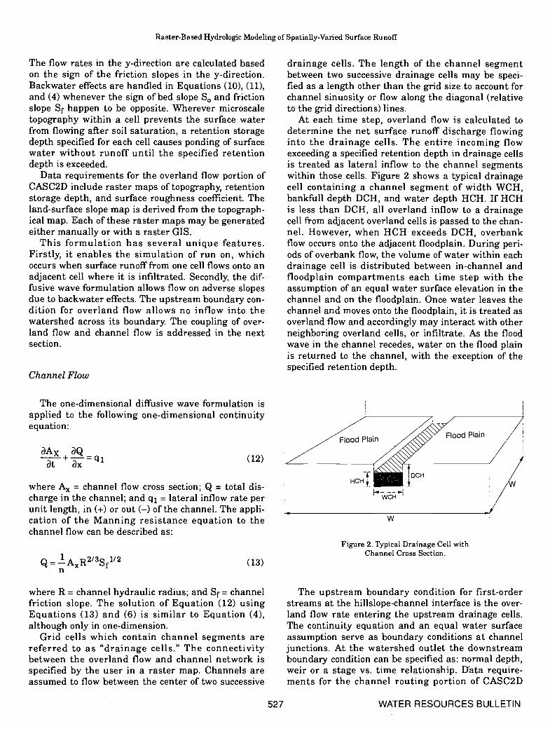
At each time step, overland flow is calculated todetermine the net surface runoff discharge flowinginto the drainage cells. The entire incoming flowexceeding a specified retention depth in drainage cellsis treated as lateral inflow to the channel segmentswithin those cells. Figure 2 shows a typical drainagecell containing a channel segment of width WCH,bankfiill depth DCH, and water depth HCH. If HCHis less than DCH, all overland inflow to a drainagecell from adjacent overland cells is passed to the chan-nel. However, when HCH exceeds DCH, overbankflow occurs onto the adjacerit floodplain. During peri-ods of overbank flow, the volume of water within eachdrainage cell is distributed between in-channel andfloodplain compartments each time step with theassumption of an equal water surface elevation in thechannel and on the floodplain. Once water leaves thechannel and moves onto the floodplain, it is treated asoverland flow and accordingly may interact with otherneighboring overland cells, or infiltrate. As the floodwave in the channel recedes, water on the flood plainis returned to the channel, with the exception of thespecified retention depth.

Figure 2. Typical Drainage Cell withChannel Cross Section.

The upstream boundary condition for first-orderstreams at the hilislope-channel interface is the over-land flow rate entering the upstream drainage cells.The continuity equation and an equal water surfaceassumption serve as boundary conditions at channeljunctions. At the watershed outlet the downstreamboundary condition can be specified as: normal depth,weir or a stage vs. time relationship. Data require-ments for the channel routing portion of CASC2D


w


include raster maps of drainage cell locations (connec-tivity), channel geometry (width, depth), and rough-ness coefficient (Manning n).

The diffusive wave channel routing formulation inCASC2D simulates backwater effects. This is particu-larly important in streams with very flat or adverseslopes. This formulation also allows flow over artifi-cial barriers due to errors in DEM data or "digitaldams" obstructing the flow in a wide cross-section.Surface water accumulates behind the barrier untilthe depth exceeds the barrier height and then spillsover. Engineering judgement is required to remove,smooth, or filter errors in DEM data bases.

MODEL FEATURES

There are three specific features which enhance theapplicability of CASC2D:

L GIS Data Link — CASC2D operates on rasterGIS-processed input data files (e.g., DEM, soil textu-ral classification, land-use and land-cover data). Todate, development has focused on the linkage ofCASC2D with the public-domain GeographicResources Analysis Support System (GRASS) GISdeveloped by the U.S. Army Construction Engineer-ing Research Laboratories in Champaign, Illinois.The CASC2D-GRASS linkage was first demonstratedby Doe and Saghaflan (1992), where GRASS capabili-ties were used to generate maps of land-surface dis-turbance at the Pinon Canyon Maneuver Site inSouthern Colorado (Doe, 1992). CASC2D is ASCII-compatible with GRASS raster maps and conceptuallycompatible with any other raster-based GIS.

2. Moving Rainstorm Input Capability - Thereare three methods to input rainfall rates in CASC2D.These methods are spatially uniform rainfall rate ofspecified duration, rainfall time-series with constanttemporal resolution at a number of rain gauges, orraster rainfall estimates with specified temporal reso-lution. Rainfall fields are interpolated from rainfallrates recorded by gauges located on or near the water-shed using either Thiessen polygon or inverse dis-tance squared techniques. Raster maps of rainfallrate from either weather radar (Ogden and Julien,1994) or space-time rainfall model sources (Ogdenand Julien, 1993) sources may be applied at a speci-fied temporal resolution.

3. Graphical Display — One of the stated objec-tives for the development of CASC2D was the desirefor visual interpretation of the rainfall-runoff process.GIS methods have allowed visual inspection of large

geophysical, geological, and other datasets. The samedisplay capability within a hydrologic modeling con-text is quite useful for educational, scientific, ariddiagnostic purposes. The graphical capabilities ofCASC2D consist of a large window which is brokeninto several sub-windows. Each sub-window displayseither a specified raster map, or a runoff hydrographat a specified point in the watershed. Versions of thegraphical display exist for both the MS-DOS andUNIX/X-Windows environments.

COMPONENT CALIBRATION/VERIFICATION

Several case studies to test the performance ofCASC2D are reported in Julien and Saghafian (1991)and are summarized here. These test cases were usedto assess the accuracy of individual components ofCASC2D (i.e., overland flow routing, channel flowrouting, and infiltration), as well as the combined per-formance of all components.

The overland flow routing component of CASC2Dwas tested against analytical solutions of the kine-matic wave equation on the one-dimensional flowplane (Woolhiser, 1975) and converging plane (Wool-hiser, 1969). Analytical solutions are available onlyfor the kinematic wave situation, and despite the factthat CASC2D employs the diffusive wave formula-tion, the diffusive wave solution becomes identical tothe kinematic wave on steeper slopes where backwa-ter effects are negligible. In each of these two cases,the numerical solution provided by the CASC2D algo-rithm is identical to the analytical solution with theexception of slight numerical diffusion near the peakon the rising limb.

The CASC2D overland flow formulation was alsocompared with multiple experimental data setsreported by Dickinson et al. (1967) for an imperviousbutyl rubber converging plane, and by Schaake (1965)for the asphalt-covered Johns Hopkins Universityparking lot. The Manning roughness coefficient wasused as the sole calibration parameter of the CASC2:Doverland flow algorithm. In this evaluation, one sub-set of each of the above data sets was used as a cali-bration data set, and the model was verified againstthe remaining data sets. CASC2D was calibrated onthe magnitude of the peak discharge. Results fromthese calibrations/verifications are shown in Table :1,and they support the validity of the formulation. Theaverage verification errors are 3 percent and —4.5 per-cent for the peak discharge and time to peak, whilethe average absolute values of the verification errorsare 4.4 percent and 4.5 percent for the peak dischargeand time to peak, respectively. The average calibra-tion error on the runoff volume at the end of the



TABLE 1. Calibration/Verification of CASC2D Overland Flow Module with ExperimentalDatasets of Dickinson et al. (1967) and of Schaake (1965).

Peak Discharge Time to PeakRunoff Volume

(at end of observed data)Observed

m3IsSimulated Error Observed Simulated

m3/s % sec. sec.Error

%Observed Simulated

me/s m3/sError

%

Data Sets by Dickinson et a!. (1967)

Calibration Run 0.0035 0.0035 0.00 156 159 1.92 0.56 0.53 —5.36

Verification Run 0.0109 0.0116 6.42 121 112 —7.44 1.21 1.27 4.96

Data Sets by Schaake et aL (1965)

Calibration Run(Storm #7)

0.0215 0.0215 0.00 426 438 2.82 14.4 13.3 —7.63

Verification Run(Storm #3)

0.0344 0.0351 1.97 1014 978 —3.55 18.8 19.9 5.85


0.0654 0.0696 6.38 672 660 —1.79 37.6 43.7 16.22


0.0277 0.0269 —2.85 702 666 —5.13 10.5 9.7 —7.62

observed data sets is —6.5 percent, while on the verifi-cation data sets it is 4.9 percent. Note that runoff vol-ume was not considered a calibration requirement.The results in Table 1 indicate that there is a tenden-cy to underestimate the time to peak by 4.5 percent.Otherwise, there are no obvious biases in the over-land flow algorithm as evidenced by the signs on theerror magnitudes with the peak discharge and runoffvolume.

The channel routing algorithm was evaluatedagainst the implicit full dynamic solution of the shal-low water equations of motion developed by Choi andMolinas (1993). The explicit channel routine wasfound to be mass-conservative and accurate comparedto the full-dynamic routing method. The performanceof the Green and Ampt formulation used in CASC2Dwas compared with a numerical solution of Richardsequation (Mein and Larson, 1971). The infiltrationalgorithm produced infiltration rate curves within afew percent of the Richards equation solution.

INDEPENDENT TESTING

Johnson et al. (1993) performed an independentcalibration and verification of CASC2D on the Good-win Creek experimental watershed in Mississippi.Calibration of CASC2D at the outlet of this basin wasverified against stream flow gauging stations withinthe basin, for a total of five different runoff events.

CASC2D was also compared with the Snyders Instan-taneous Unit Hydrograph (SIUH) and SCS CurveNumber (CN) approaches in HEC-1, using Musk-ingum-Cunge channel routing. These researchersconcluded that CASC2D consistently performed aswell or better than either the SIUH or CN HEC-1approaches on the Goodwin Creek dataset. The pri-mary calibration parameters used include initial soilmoisture deficit, channel roughness coefficient, reten-tion storage depth, and overland flow roughness coef-ficient. They also concluded that CASC2D alwaysproduced more accurate hydrographs on simulatedungauged basins (from the parametric values of Man-ning n and infiltration based on soil types without cal-ibration).

STABILITY AND NUMERICAL ACCURACY

The stability of CASC2D was examined during thedevelopment (Saghafian, 1992; Julien and Saghafian,1991). In summary, the explicit overland and channelflow algorithms require relatively small time steps forstability. The optimum time step depends upon thegrid size, rainfall intensity, rainfall duration, bothaverage and local bed slopes in the basin, surfaceroughness, and infiltration parameters. Specifically,the Courant condition evaluated under peak dis-charge conditions, which is the critical state withmaximum flow velocity, provides a preliminary time



step value. The maximum time step for which themodel is stable should be used because optimum solu-tion convergence is achieved when the Courant num-ber is near 1.0. Numerical stability is achieved ontypical grid sizes with time steps between 5 and 60seconds.

Situations which are particularly difficult to modelwith the CASC2D channel routing formulationinclude narrow channels with substantial changes inbed slope or channel cross-section. These can causenumerical instability in the transfer of water betweenthe channel and floodplain during periods of overbank flow.

Surfaces with highly irregular microtopography atscales much smaller than the grid size do not pose aproblem. Tayfur et al. (1993) found that replacing spa-tially varying microtopography with an average con-stant slope and appropriate retention storage causesno significant changes in the outflow hydrograph butdoes cause substantial deviations in local flow depthsand velocities. Therefore, the user should be cau-tioned regarding the accuracy of flow velocity calcula-tions within individual grid cells.

EXAMPLE APPLICATIONS OF CASC2D

The following two sections present example appli-cations of CASC2D. The first section is an applicationof CASC2D with rainfall data from a dense raingaugenetwork during a calibration run. The second sectionpresents a brief discussion of contemporary weatherradar rainfall rate estimation techniques and illus-trates the applicability of weather radar estimatedrainfall within CASC2D.

Modeling of Macks Creek Experimental Watershedwith Raingauge Data

Macks Creek, a 32.2 km2 sub-basin of the ReynoldsCreek Experimental Watershed, is a steep semi-aridwatershed located in southwest Idaho. A contour plotof Macks Creek is shown in Figure 3, with a 1 km gridoverlay as a scale reference. The elevation drops from1830m in the mountains along the western edge to1130m at the outlet which is located in the northeastcorner of the watershed. Two main channels, each

Figure 3. Macks Creek Watershed Topography and Channel Network.


Macks Creek Watershed., Idaho

Contour IntervalGrid Size 1 km

30 m


with slopes averaging 5 percent and lengths near 10km, collect surface runoff. The channel network isshown on Figure 3 with heavy lines. Note the longestcontinuous channel which drains the southern portionof the watershed and flows approximately from south-west to northeast. The second main channel drainsthe northern portion of the watershed, and flows in aroughly easterly direction.

For this particular calibration run the storm ofAugust 23, 1965, was selected. Rainfall data with two-minute resolution was recorded by eight raingaugeslocated on or near the watershed. The recorded accu-mulated rainfall depth over the two-hour stormreached 1.65 cm at one gauge, with a maximum rain-fall rate over a two-minute period exceeding 20 cm/hr.Inverse distance squared weighting was applied tointerpolate rainfall fields from the raingauge data.Outflows were recorded at a pre-calibrated 100 m3/scapacity drop box weir at the watershed outlet on 15-minute intervals. A base flow of approximately 0.023m3/s at the outlet was neglected in the view of the 2.4m3/s measured peak discharge.

The geographical region containing the watershedwas divided into a 53 x 53 grid, with a grid size of 152m. The watershed mask contains 1390 grid cells. Inthis instance, the topography of Macks Creek wasmanually digitized to produce a raster DEM at a gridsize of 152 m. The SCS soil classification map ofMacks Creek was digitized by Cline (1988) at thissame grid size. Both digitized maps were entered inthe GRASS GIS for storage, editing, and export toCASC2D.

Values of hydraulic conductivity and capillary drivebased on soil textural classificatiOn were used as rec-ommended by Rawis et al. (1983). Antecedent soilmoisture conditions were assumed near-dry owing tothe semi-arid climate of the region, the absence of anysubstantial rainfall on the preceding day, and the neg-ligible base flow at the weir. A spatially uniform valueof Manning n for overland flow equal to 0.06was used, which is within the range proposed byWoolhiser (1975) for sparse vegetation. The calibra-tion parameters selected for this example are surfaceroughness and initial soil moisture deficit. Adequacyof this particular calibration was judged based on thetiming and magnitude of the peak discharge, as wellas the total runoff hydrograph volume.

Figure 4 shows the CASC2D visual display at 20,35, 70, and 239.5 minutes during the model run. Eachvisual display is further broken down into sub-win-dows. The upper left sub-window shows the rainfallrate over the watershed, while the upper right sub-window depicts the surface water depth in eachgrid cell. The lower left and right sub-windows,respectively, display the cumulative infiltrated depthand the outflow hydrograph. The purple dots on the

hydrograph sub-window represent observed dischargemeasurements at the weir.

With reference to the upper left quadrant of Fig-ure 4, the storm is approaching the southeastern bor-der of the watershed at t = 20 minutes. Note that atthis point in the model run, the surface water depth iszero everywhere with the exception of a few rock out-crops along the western edge of the catchment. Theclassic "egg yolk" features in the interpolated rainfallfield are the result of the inverse-distance squaredrainfall interpolation scheme. Referring to the topright quadrant of Figure 4, at t = 35 minutes, thestorm has moved to the northwest and intensifiedover the northeastern portion of the watershed.Accordingly, the cumulative infiltrated depth and sur-face water depth windows illustrate the partitioningof the rainfall into soil and surface water components.Note the partial areas of contribution in the surfacewater depth map.

As this particular storm unfolds, no surface runoffis generated from the southern third of the water-shed. With reference to the lower left quadrant of Fig-ure 4, at t = 70 minutes, there is no surface water inthis portion of the watershed. At this time the hydro-graph peak has just reached the catchment outlet.The short-duration high-intensity rainfall on thenorthern portion of the watershed is responsible forthis sudden flashilood. In the lower right quadrant ofFigure 4, at t = 239.5 minutes, all surface water isnow limited to channel flow draining slowly towardthe outlet. As evidenced by the hydrograph plot, fairagreement is observed between the computed hydro-graph (solid red line) and the observed hydrograph(purple dots). Given the 15-minute temporal resolu-tion of the recorded outflow hydrograph and theflashy response of Macks Creek, there is considerableuncertainty regarding the magnitude and timing ofthe measured hydrograph peak. Overall, this calibra-tion run demonstrates that surface runoff is generat-ed on partial areas of the watershed (northern partin this case). The model can accurately simulate sur-face runoff from flashfloods caused by intense thun-derstorms moving across partial areas of a watershed.

Example Application of CASC2D with WeatherRadar Estimated Rainfall

This section illustrates a CASC2D runoff simula-tion using real weather radar rainfall rates applied toa watershed at a different location. Weather radarobservations of a convective storm over the plains ofeastern Colorado are converted to rainfall rate esti-mates and used as input to CASC2D on the MacksCreek, Idaho, experimental watershed, which wasdiscussed in the previous section. This simulation



Figure 4. CASC2D Calibration on Macks Creek Using Raingauge Data at t = 20 Mm. (upper left),35 Mm. (upper right), 70 Mm. (lower left), and 239.5 Mm. (lower right).

illustrates how CASC2D can interface with radardata, although, without comparison of the simulationresults with an actual runoff hydrograph.

The raster formulation of CASC2D readily acceptsraster estimates of rainfall rate at any spatial resolu-tion. Raster rainfall estimates may be derived frominterpolated raingauge data or isohyetal maps,weather radar or satellite observations, or space-timestochastic rainfall models. The only requirement isthat the rainfall raster grid size must be evenly divisi-ble by the runoff model grid size. For this reason, theelevation and soil classification maps of Macks Creekwere re-digitized at a resolution of 125 m. Rainfalldata grid size considerations and related scalingissues are discussed at length by Ogden and Julien(1994).

This example simulation relies upon CSU-CHILLweather radar observations of a convective rainstorm


at five-minute intervals and 1 km spatial resolution.The CSU-CHILL radar is a research facility jointlyfunded by the National Science Foundation and Col-orado State University. It operates at a non-attenuat-ing wavelength of 10 cm (frequency = 2.95 GHz), hasa 1 degree beam-width, and has dual-linear polariza-tion and Doppler capabilities. For this example theradar measurements (Reflectivity, Differential Reflec -tivity, and Specific Differential Propagation PhaseShift) were converted into rainfall rate using themethod detailed in Ogden and Julien (1994) andOgden (1992). Readers interested in advanced radar.rainfall estimation techniques are referred to discus-sions by Zawadzki (1982), Sachidananda and Zrnic(1987), Chandrasekar et at. (1990, 1993), Gorgucci etat. (1994), and Aydin et al. (1995).

The CSU-CHILL radar monitored a convectivestorm on June 3, 1991. The radar measurements were


Figure 5. CASC2D Simulation on Macks Creek Using Weather Radar Estimated Rainfall att = 50 Mm. (upper left),75 Mi (upper right), 110 Mm. (lower left), and 235 Mm. (lower right).

recorded in spherical coordinates, with 300 m spatialresolution in the direction of the radar beam, and 1degree resolution in the azimuthal and elevationangle directions. Radar scans at a beam elevationangle of 1 degree above the horizon were completedonce per five minutes over the duration of the storm,which lasted about 150 minutes. After conversion torainfall rates in spherical radar coordinates, the rain-fall estimates were converted onto a 1 km x 1 kmraster grid using a minimum-curvature spline tech-nique.

Similar to Figure 4, Figure 5 shows a visual displayof CASC2D with weather radar estimated rainfall atfour different times during the simulation (50, 75,110, and 235 minutes respectively). The CASC2Dgraphical display with radar-estimated rainfall is dif-ferent from the display with raingauge rainfall.

Specifically, the upper-left sub-window was added toillustrate the spatial variability of rainfall within alarge radar domain around the watershed, which is80 x 80 km in size. The location of the watershedwithin this sub-window is bounded by a white rectan-gle, and the radar is located near the center of thesub-window. For this illustrative example, the loca-tion of the watershed within the radar domain waschosen arbitrarily.

With reference to the visual display shown in theupper left quadrant of Figure 5, at simulation timet = 50 minutes after the beginning of simulation, thestorm can be seen building west of the watershedlocation in the radar domain sub-window. The spatialvariability of the 1 km raster rainfall field overthe watershed is shown in the upper-middle sub-win-dow. The light blue pixel in the watershed rainfall



sub-window indicates a rain rate between 30 and 40mm/h on the very western edge of the basin. Theupper-right and lower-right sub-windows detail thesurface water and cumulative infiltrated depths,respectively, at this point in the simulation. Note thesimilarity with the graphical displays in Figure 4with regard to the rocky outcrops along the westernedge of the watershed. The surface depth map indi-cates ponded conditions on the rocky areas while thecumulative infiltrated depth map indicates no infil-tration.

Referring to the upper right quadrant of Figure 5,at t = 75 minutes, the convective storm can be seendirectly over the watershed in the upper left sub-window. The upper-middle sub-window shows one1 km x 1 km region (yellow rainfall pixel) receiving anestimated rainfall rate between 120 and 140 mm/h.The upper right sub-window shows that the overlandflow in the southwestern portion of the watershed isbeginning to accumulate in the channel network,while the lower right sub-window shows a significantincrease in infiltrated depth, particularly in thenortheastern corner of the watershed, where it is nowraining most heavily. The hydrograph display andsimulation summary box in the lower portion of thevideo display indicate that runoff has not yet reachedthe outlet.

The video display in the lower-left quadrant of Fig-ure 5 shows the state of the simulation at t = 110 min-utes. As seen in the radar domain sub-window, thebulk of the storm has passed east of the watershedlocation. The upper-middle sub-window shows thatrainfall rates less than 30 mm/h continue to fall in theextreme northeast corner of the watershed, whilelight rainfall less than 10 mm/h covers the centralportion of the catchment. The surface depth mapshows significant accumulations of water in the chan-nel network with a flood wave moving toward the out-let in each of the two main channels. The cumulativeinfiltration map shows significant cumulative infiltra-tion in the middle and eastern portions of the water-shed, while the simulation status box in the extremelower-right corner indicates the present outflow rateis 0.09 m3/s.

The lower right quadrant of Figure 5 shows theCASC2D visual display at a simulation time of 235minutes. The radar domain sub-window indicates noprecipitation in the area or on the watershed. Thesurface water depth sub-window shows that all sur-face waters have infiltrated except in some channels,floodplains, and rocky regions. Furthermore, this win-dow shows that the flood waves from both main chan-nels have passed through to the outlet. The resultinghydrograph from this storm is shown in the lower-leftsub-window, and the simulation summary sub-win-dow indicates a peak discharge of 36.99 m3/s passed


the outlet at t = 184 minutes. Note the degree of spa-tial detail available at the end of the simulationregarding the location of flood waters, and spatialvariability of cumulative infiltrated depth. This infor-mation could be most useful for the initiation of a newsimulation if a second storm were to be headedtoward the watershed.

SUMMARY AND CONCLUSIONS

Recent developments and increasing usage of GIStechnology for the storage and retrieval of watershedcharacteristics in raster format enhance hydrologicalmodels that can fully access these data sources. GIStechnology has also shown the educational, scientific,and diagnostic value of visual displays of large datasets. Furthermore, the increasing availability ofweather radar rainfall estimates in raster format alsonecessitates the development of hydrological modelscapable of incorporating spatially-varied rainfallwhile preserving the spatial and temporal informa-tion provided by weather radars.

This paper outlines the details of the model formu-lation and list assumptions pertaining to the develop-ment and verification of the components. Thecalibration and accuracy of CASC2D are discussedtogether with numerical stability and model limita-tions. Two example applications which simulate theresponse of the 32.2 km2 Macks Creek experimentalwatershed in southwestern Idaho are presented. Thefirst application illustrates a CASC2D calibration runwith rainfall rates interpolated from a dense networkof raingauges. The second example illustrates the linkbetween CASC2D and radar-estimated rainfall. Inboth examples, the utility of the graphical display inrelating the state of a simulation to the user is dis-cussed.

The accuracy of the overland flow, infiltration, andchannel routing components of CASC2D has beenassessed independently. CASC2D produces runoffhydrographs which are generally more accurate thaneither the SCS CN or Snyders Instantaneous UnitHydrograph approaches with Muskingum Cungechannel routing in HEC-1. The unique visual displaycapability of CASC2D allows the user unprecedentedaccess to the entire simulation while it is in progress.The visual display essentially provides CASC2D usersaccess to the results of the simulation as it unfolds.This capability has potential for practical as well asresearch applications. The model is particularly well••suited to the simulation of flashfloods from intensethunderstorms moving across partial areas of awatershed.


In conclusion, the physically-based distributednature of CASC2D makes it a suitable modeling toolto carry out fundamental research on spatially-variedsystems. CA1SC2D features include GIS compatibility,direct link with remotely-sensed rainfall data, accura-cy of simulation, and unique graphical interface. Thepaper presents innovative applications of recentadvances in computational hydrology. As illustratedin Figure 4, the model can accurately simulate sur-face runoff from flashfloods caused by intense thun-derstorms moving across partial areas of a watershed.

ACKNOWLEDGMENTS

This study was completed at the Engineering Research Centerwithin the Center for Excellence in Geosciences at Colorado StateUniversity. Financial support by the U.S. Army Research Office(Grant ARO/DAAL 03-86-0175) is gratefully acknowledged. Weappreciate the technical assistance of Drs. J. S. O'Brien, W. Doe Ill,0. R. Stein, Y. Q. Lan, K. Marcus, and G. Choi at the time themodel was developed. Our gratitude is extended to Dr. W. Bach forhis continuous support of this research program.

LiTERATURE CiTED

Abbott, M. B., J. C. Bathurst, J. A. Cunge, P. E. O'Connell, andJ. Rasmussen, 1986. An Introduction to the European Hydrolog-ical System — Système Hydrologique Europeen, "SHE." 2: Struc-ture of a Physically-Based, Distributed Modelling System,Journal of Hydrology 87:61-77.

Aydin, K., V. N. Bringi, and L. Liu, 1995. Rain Rate Estimation inthe Presence of Hail Using S-band Specific Differential Phaseand Other Radar Parameters, Journal AppI. Meteorol. 34(2) (InPress).

Chandrasekar, V., V. N. Bringi, N. Balakrishnan, and D. S. Zrnic,1990. Error Structure of Multiparameter Radar and SurfaceMeasurements of Rainfall. Part III: Specific Differential Phase.Journal Atmos. Oceanic Technol. 7(5):621-629.

Chandrasekar, V., E. Gorgucci, and G. Scarchilli, 1993. Optimiza-tion of Multiparameter Radar Estimates of Rainfall. JournalAppi. Meteorol. 32(7):1288-1293.

Choi, G. W. and A. Molinas, 1993. Simultaneous Solution Algorithmfor Channel Network Modeling. Water Resources Research29(2):321-328.

Cline, T. J., 1988. Development of a Watershed Information Systemfor HEC-1 with Application to Macks Creek, Idaho. M.S. Thesis,Civil Engineering Dept., Colorado State University, Fort Collins,Colorado, 238 pp.

Cline, T. J., A. Molinas, and P. Julien, 1989. An Auto-CAD-BasedWatershed Information System for the Hydrologic ModelHEC-1. Water Resources Bulletin, 25(3), pp. 641-652.

DeVantier, B. A. and A.D. Feldman, 1993. Review of GIS Applica-tions in Hydrologic Modeling. Journal of Water Resources Plan-ning and Management, ASCE, 119(2):246-261.

Dickinson, W. T., M. E. Holland, and G. L. Smith, 1967. An Experi-mental Rainfall-Runoff Facility. Hydrology Paper No. 25, Col-orado State University, Fort Collins, Colorado.

Doe, W. W, 1992. Simulation of the Spatial and Temporal Effects ofArmy Maneuvers on Watershed Response. Ph.D. Dissertation,Civil Engineering Dept., Colorado State University, Fort Collins,Colorado, 301 pp.

Doe, W. W. and B. Saghafian, 1992. Spatial and Temporal Effects ofArmy Maneuvers on Watershed Response: The Integration of

GRASS and a 2-D Hydrologic Model. Proc. 7th Annual GRASSUsers Conference, National Park Service Technical ReportNPS/NRG15D/NRTR-93/13, Lakewood, Colorado, pp. 91-165.

Goodrich, D. C., D. A. Woolhiser, and T. 0. Keefer, 1991. KinematicRouting Using Finite Elements on a Triangular Irregular Net-work. Water Resources Research 27(6):995- 1003.

Gorgucci, E., G. Scharchilli, and V. Chandrasekar, 1994. A RobustPointwise Estimator of Rainfall Rate Using Differential Reflec-tivity. Journal Atmos. Oceanic. Tech. 11(2):586-592

James, W. P. and K. W. Kim, 1990. A Distributed Dynamic Water-shed Model. Water Resources Bulletin 26(4):587-596.

Johnson, B. E., N. K. Raphelt, and J. C. Willis, 1993. Verification ofHydrologic Modeling Systems. Proc. Federal Water AgencyWorkshop on Hydrologic Modeling Demands for the 90's, USGSWater Resources Investigations Report 93-4018, June 6-9, Sec.8., pp. 9-20.

Julien, P. Y. and B. Saghafian, 1991. A Two-Dimensional WatershedRainfall-Runoff Model. Civil Engr. Report, CER9O-9IPYJ-BS-12, Dept. of Civil Engineering, Colorado State University, FortCollins, Colorado, 63 pp.

Kiazura, G. E. and D. A. Imy, 1993. A Description of the Initial Setof Analysis Products Available from the NEXRAD WSR-88DSystem. Bull. Am. Meteor. Soc., 74(7):1293-1311.

Marcus, K. B., 1991. Two-Dimensional Finite Element Modeling ofSurface Runoff from Moving Storms on Small Watersheds.Ph.D. Dissertation, Civil Engineering Dept., Colorado StateUniversity, Fort Collins, Colorado.

Mein, R. G. and C. L. Larson, 1971. Modeling the Infiltration Com-ponent of the Rainfall-Runoff Process. Bulletin 43, WaterResources Research Center, University of Minnesota, Minneapo-lis, Minnesota.

Ogden, F. L., 1992. Two-Dimensional Runoff Modeling with Weath-er Radar Data. Ph.D. Dissertation, Civil Engineering Dept., Col-orado State University, Fort Collins, Colorado., 211 pp.

Ogden, F. L. and P. Y. Julien, 1993. Runoff Sensitivity to Temporaland Spatial Rainfall Variability at Runoff Plane and SmallBasin Scales. Water Resources Research 29(8):2584-2597.

Ogden, F. L. and P. Y. Julien, 1994. Runoff Model Sensitivity toRadar-Rainfall Resolution. Journal of Hydrology 158:1- 18.

Rawls, W. J., D. L. Brakensiek, and N. Miller, 1983. Green-AmptInfiltration Parameters from Soils Data. Journal of HydraulicEngineering, ASCE 109(1):62-70.

Sachidananda, M. and D. S. Zrnjc, 1987. Rain Rate Estimates fromDifferential Polarization Measurements. Journal of Atmos. andOceanic Tech 4:588-596.

Saghafian, B., 1992. Hydrologic Analysis of Watershed Response toSpatially Varied Infiltration. Ph.D. Dissertation, Department ofCivil Engineering, Colorado State University, Fort Collins, Col-orado.

Schaake, J. C., 1965. Synthesis of the Inlet Hydrograph. Ph.D. Dis-sertation, Dept. of Sanitary Engineering and Water Resources,The Johns Hopkins University, Baltimore, Maryland.

Tayfur, G., M. L. Kavvas, R. S. Govindaraju, and D. E. Storm, 1993.Applicability of St. Venant Equations for Two-DimensionalOverland Flows Over Rough Infiltrating Surfaces. Journal ofHydraulic Engineering, ASCE 119( 1):5 1-63.

Vieux, B. E., 1991. Geographic Information Systems and Non-PointSource Water Quality and Quantity Modeling. Hydrological Pro-cesses 5:10 1-113.

Woolhiser, D. A., 1969. Overland Flow on a Converging Surface.Trans. of ASAE, 12(4):460-462.

Woolhiser, D. A., 1975. Simulation of Unsteady Overland Flow. In:Unsteady Flow in Open Channels, Vol. II, Chapter 12, K. Mah-mood and V. Yevjevich (Editors). Water Resources Publications,Fort Collins, Colorado.

Zawadzki, I, 1982. The Quantitative Interpretation of WeatherRadar Measurements; Atmos. Ocean 20:158-180.

Zhang, W. and T. W. Cundy, 1989. Modeling of Two-DimensionalOverland Flow. Water Resources Research 25(9):2019-2035.


Julien, Saghaflan, and Ogden

NOTATIONS

E = ground elevation

f = infiltration rate

F = cumulative infiltration depth

g = gravitational acceleration

h = flow depth= capillary pressure head at the wetting front

= rainfall intensity= excess rainfall intensity

j = rownumberofgridcellk = column number of grid cellL = total length along hydraulically longest kinematic flow

pathMa = soil moisture deficit

n = Manning roughness coefficient

q = unit discharge

q1 = lateral inflow

= unit discharge in the x,y directions

Q = total dischargeR = hydraulic radiusS = degree of initial soil saturation

S0 = bed slope

Sf = friction slopet = time

V = flow velocityW = overland plane width

x,y = Cartesian coordinates

,13,y = parameters of the resistance equations= the effective soil porosity

= initial soil moisture content

= residual saturation= total soil porosity


Documents

RASTER-BASED HYDROLOGIC MODELING OF SPATIALLY-VARIED SURFACE RUNOFF