Rate and Extent of Digestion - basu.ac.ir and extent of... · 2 Rate and Extent of Digestion D.R. Mertens ... of total tract digestibility and is the first step in the digestive process

2 Rate and Extent of Digestion

D.R. Mertens

USDA – Agricultural Research Service, US Dairy Forage Research Center,Madison, WI 53706, USA

Introduction

Digestion in ruminants is the result of two competing processes: digestion andpassage. Rate of passage determines the time feed is retained in the alimentarytract for digestive action and the rate and potential extent of degradationdetermines the digestion that can occur during the retention time. To predictdynamic flows of nutrients or static estimates of digestibility at various levels ofperformance, the processes of digestion and passage must be described incompatible mathematical terms and integrated. This chapter will focus on themathematical description or modelling of digestion, especially fermentativedigestion in the rumen because it typically represents the largest proportionof total tract digestibility and is the first step in the digestive process forruminants that influences the processes that follow.

The digestive process involves the time-dependent degradation or hydroly-sis of complex feed components into molecules that can be absorbed by theanimal as digesta passes through the alimentary tract. Conceptually, digestionand passage can be described as multi-step processes using compartmentalmodels (Blaxter et al., 1956; Waldo et al., 1972; Baldwin et al., 1977, 1987;Mertens and Ely, 1979; Black et al., 1980; Poppi et al., 1981; France et al.,1982). Because feed components do not digest or pass through the digestivetract similarly (Sutherland, 1988), an understanding about the nature of pas-sage in ruminants provides an important framework for developing compatibledigestion models.

In ruminants, passage of digesta through the alimentary tract is a complexprocess that involves selective retention, mixing, segregation, and escape ofparticles and liquid from the rumen before they pass into and through the smalland large intestines. Mechanistically, the reticulorumen, small intestine andlarge intestine differ in mixing and flow. The rumen operates as an imperfectlystirred, continuous-flow reactor, whereas the small and large intestines act

� CAB International 2005. Quantitative Aspects of Ruminant Digestionand Metabolism, 2nd edition (eds J. Dijkstra, J.M. Forbes and J. France) 13

more like plugged-flow reactors (Levenspiel, 1972; Penry and Jumars, 1987).Furthermore, ruminal contents act as though there were at least three differentsubcompartments with different flow characteristics: liquid, escapable particlesand retained particles. Soluble feed components dissolve and pass out at therate of ruminal liquids. Ground concentrates and forages pass out of the rumenmore quickly than large fibre particles, which are retained selectively andruminated. Models of digestion must be compatible with these differences inpassage rates and processes.

Separate compartments are needed to represent the distinct digestive andpassage processes of the reticulorumen, small intestine and large intestine. Theunique digestive kinetics of feed components should be described by dividingfeed into rapidly digested, slowly digested and indigestible compartments. Thevariety of compartments needed to model digestion and passage illustrates animportant principle. Model compartments are defined by their kinetic proper-ties and may not necessarily correspond to anatomical, physiological, chemicalor physical compartments in the real system. Thus, non-escapable and escap-able particles should be described as separate compartments, though both arein the ruminal environment. The kinetic property of ‘escapability’ rather thanparticle size is used to define particles because small particles trapped in thelarge particle ruminal mat pass differently from those located in the reticular‘zone of escape’ (Allen and Mertens, 1988). Particles are uniquely definedbecause they have different kinetic parameters and require separate equationsto describe the processes of digestion and passage. Similarly, digestible andindigestible matter may be contained in the same feed particle, yet eachrequires a separate compartment to describe their unique kinetics of digestionand passage.

Current models describe digestion as a function of the mass of substratethat is available in a compartment, i.e. they are mass-action models. Generally,digestion is described as a first-order process with respect to substrate (Waldoet al., 1972; Mertens and Ely, 1979); however, some models describe it as asecond-order process that depends on the pools of substrate and microorgan-isms present in the system (France et al., 1982; Baldwin et al., 1987).Regardless of the model used, it appears that rate and extent of digestion arecritical variables in the description of the digestion process. Kinetic parametersof digestion are important because they not only describe digestion, but alsothey characterize the intrinsic properties of feeds that limit their availability toruminants.

To be useful, models based on mechanistic assumptions must replicate thereal system with an acceptable degree of accuracy. The number of differentmechanistic models that can predict a set of observations may be large, per-haps infinite (Zierler, 1981). Thus, accuracy in predicting a specific set of datacannot prove that a model is uniquely valid, but only indicates that it is oneplausible explanation of reality. To be universally applicable, models should bevalid in extreme situations and under varied experimental conditions, ratherthan predicting the average accurately, even if it is from a large data set.

The goal of this chapter is to present the theoretical development and useof models for quantifying rate and extent of the digestion process in the rumen.

14 D.R. Mertens

To accomplish this goal, methods used to collect kinetic data will be analysed,the background of simple models for measuring rate and extent of fermentativedigestion will be discussed, mathematical models will be proposed that moreaccurately describe the methods used to obtain kinetic data, and methods offitting data to models for estimating kinetic parameters will be reviewed.

Terminology

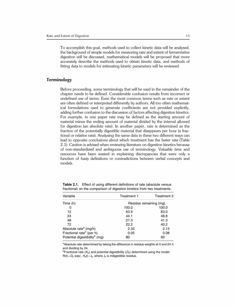
Before proceeding, some terminology that will be used in the remainder of thechapter needs to be defined. Considerable confusion results from incorrect orundefined use of terms. Even the most common terms such as rate or extentare often defined or interpreted differently by authors. All too often mathemat-ical formulations used to generate coefficients are not provided explicitly,adding further confusion to the discussion of factors affecting digestion kinetics.For example, in one paper rate may be defined as the starting amount ofmaterial minus the ending amount of material divided by the interval allowedfor digestion (an absolute rate). In another paper, rate is determined as thefraction of the potentially digestible material that disappears per hour (a frac-tional or relative rate). Analysing the same data in these two different ways canlead to opposite conclusions about which treatment has the faster rate (Table2.1). Caution is advised when reviewing literature on digestion kinetics becauseof non-standardized and ambiguous use of terminology. Valuable time andresources have been wasted in explaining discrepancies that were only afunction of fuzzy definitions or contradictions between verbal concepts andmodels.

Table 2.1. Effect of using different definitions of rate (absolute versusfractional) on the comparison of digestion kinetics from two treatments.

Variable Treatment 1 Treatment 2

Time (h) Residue remaining (mg)0 100.0 100.0

12 63.9 63.024 44.1 48.848 27.3 41.372 22.2 40.2

Absolute ratea (mg/h) 2.33 2.13Fractional rateb (per h) 0.05 0.08Potential digestibilityb (mg) 80 60

aAbsolute rate determined by taking the difference in residue weights at 0 and 24 h

and dividing by 24.bFractional rate (Kd) and potential digestibility (D0) determined using the model

R(t)¼D0 exp(�Kdt)þI0, where I0 is indigestible residue.

Rate and Extent of Digestion 15

The following are definitions of terms used in this chapter:

Aggregation: Combining entities or attributes in a model that have similarkinetic properties to reduce detail and complexity.

Assumptions: Implicit or explicit relationships or attributes of a model that areaccepted a priori.

Attributes: Coefficients of parameters and variables used to describe theentities in a model.

Compartment: Boundaries of an entity that is distributed in an environmentthat is assumed to have homogeneous dynamic or static properties. Com-partments are typically represented in diagrams by solid-lined boxes.

Dynamic: Systems, reactions or processes that change over time.Entities: Independent, complete units or substances that have uniquely defined

chemical or physical properties in a system.Environment: Physical location of an entity in a system.Extent of digestion: A digestion coefficient that represents the proportion of a

feed component that has disappeared as a result of digestion after aparticular time in a specified system. It is a function of the time allowedfor digestion and the digestion rate. Units are fractions or percentages.Extent of digestion is a more general term that is not equal to either thepotentially digestible fraction or potential extent of digestion.

Flux or flow: Amount of material per unit of time that is transferred to or froma compartment. In non-steady-state conditions, fluxes vary over time.Although they may have the same mathematical form in some cases, fluxesare not the same concept as the derivative of the pool size. Fluxes typicallyare represented in diagrams by arrows.

Flux ratio: Proportion of a flux that is transferred to or from a compartment.Flux ratios differ conceptually from fractional rates because ratios partitionfluxes, whereas rates are proportions of pools that are transferred. Fluxratios typically are represented in mathematical equations by lower case ‘r’with a subscript.

Indigestible residue: Residue of feed that remains after an infinite time ofdigestion in a specified system. It is often approximated by measuring thedisappearance of matter after long times of digestion.

Kinetics, mass-action: Systems in which material is transferred between com-partments in proportion to the mass of material in each compartment.

Kinetics, Michaelis–Menten (or Henri–Michaelis–Menten): Kinetics derivedfrom a reversible second-order mass-action system in which the flux ofproduct formation is proportional to the concentration of substrate andenzyme (or microbial mass). With respect to substrate, the reaction variesfrom zero-order when enzyme is limiting, to first-order when enzyme (ormicrobial mass) is in excess.

Models: Representations of real-world systems. Models do not duplicate thereal world because they always contain assumptions about, and aggrega-tions of, components of the real-world system. Mathematical models useexplicit equations to describe a system.

16 D.R. Mertens

Models, deterministic: Assume the system can be simulated with certaintyfrom known or assumed principles or relationships.

Models, dynamic: Simulate the change in the system over time.Models, empirical: Based on relationships derived directly from observations

about the system. These data-driven models are sometimes called black boxor input–output models.

Models, kinetic: Kinetics refers to movement and the forces affecting it. Inchemical and biological systems, kinetic models are related to the molecu-lar movement associated with chemical or physical systems.

Models, mechanistic: Are based on known or assumed biological, chemical orphysical theories or principles about the system. These concept-drivenmodels are sometimes called white box models.

Models, static: Represent time-invariant systems or processes. The steady-state solution of dynamic systems is a specific type of static model.

Models, stochastic: Assume that the system operates on probabilistic prin-ciples or contains random elements that cannot be known with certainty.

Order of reaction: The combined power terms of the pools in mass-actionkinetic systems. For example, in first-order systems the flux of reaction isrelated to the amount or concentration of a single pool raised to the power1. In second-order systems, flux is related to a single pool raised to thepower 2 or the product of two pools raised to the power 1.

Parameters: Constants in equations that are not affected by the operation ofthe model.

Pool: Mass, weight or volume of material in a compartment. Pools are typicallyrepresented by upper case letters in mathematical equations.

Potentially digestible fraction: Inverse of the indigestible fraction (1.0 –indigestible fraction). It is the proportion of feed that can disappear dueto digestion given an infinite time in a specified system. The potentiallydigestible fraction is the same as the potential extent of digestion ormaximal extent of digestion.

Processes: Activities or mechanisms that connect entities within a system anddetermine flows or fluxes between compartments.

Rate: Change per unit of time, which can be expressed in many different units;therefore, it is important to indicate the specific type of rate being dis-cussed, preferably with a mathematical description.

Rate, absolute: Has the units of mass per unit of time. Absolute rates andfluxes are the same, but the term ‘flux’ is preferred because it preventsconfusion associated with the unqualified use of the term ‘rate’.

Rate, first-order: Fractional rates that are proportional to a single pool.Rate, fractional (or relative): Proportion of mass in a pool that changes per

unit of time. This rate has no mass units and is usually a constant that doesnot vary over time. First-order fractional rate constants are usually repre-sented in mathematical equations by a lower case ‘k’ with subscripts.

Simulation: Operation of a model to predict a result expected in the real-worldsystem.


Sinks: Irreversible end-point compartments of entities that are outside opensystems. Sinks are typically represented in diagrams by clouds with enter-ing arrows.

Sources: Initial locations of materials that are supplied from outside opensystems. Sources are typically represented in diagrams as clouds withexiting arrows.

State, quasi-steady: Occurs when pools within compartments in a dynamicsystem do not change significantly. Under natural situations, the timeneeded to attain quasi-steady-state is relative. True steady state cannot beachieved in perturbed systems because small changes are occurring con-tinuously. Quasi-steady-state is sometimes called the steady-state approxi-mation.

State, steady: Occurs when pools within compartments in a dynamic systemdo not change. True steady state is a mathematical construct that occurswhen the derivative of a pool with respect to time equals zero.

Systems: Organized collections of entities that interact through various pro-cesses. Open systems can accept or return material outside the system,whereas all material must originate and be retained in a closed system.

Time, retention: Is the average time an entity is retained in a compartment.Time, turnover: Is the time needed for a compartment to transfer an amount

of material equal to its pool size.Validation: Evaluating the credibility or reliability of a model by comparing it to

real-world observations. No model can be validated completely because allof the infinite possibilities cannot be evaluated. Some modellers prefer theterm ‘evaluation’ rather than ‘validation’.

Variables: Coefficients that change during or among model simulations. Vari-ables can be external or internal to the model. External or exogenousvariables are inputs that affect or interact with the system that is modelled,but are controlled outside of it. Internal or endogenous variables are calcu-lated within the model during its operation.

Variables, state: Define the level, mass or concentration within the pools of thesystem.

Verification: Checking the accuracy by which a model is described mathemat-ically and implemented.

Requirements for Quantifying Rate and Extent of Digestion

Robust quantitative description of the rate and extent of digestion requiresthree components:

1. Appropriate biological data measured in a defined, representative systemusing an optimal experimental design.2. Proper mathematical models that reflect biological principles.3. Accurate fitting procedures for parameter estimation.

The validity of digestion kinetics depends on data that are accurately collected ina relevant system.Once the biology of the system for collecting data is described,

18 D.R. Mertens

models should be developed that correctly reflect the system. Only then can avalid fitting procedure be used to accurately estimate rate and extent of digestion.

Kinetic Data

Accurate biological data, generated by a method that is consistent with themathematical model and its assumptions, is a necessary first step in quantifyingdigestion kinetics. Subtle differences among measurements can have substan-tial effects on the parameterization and interpretation of digestion kinetics.Three characteristics of the data have critical impact on modelling and theinterpretation of kinetic properties:

1. The method used to measure kinetic changes.2. The specific component on which kinetic information is measured.3. The design of sampling times and replications.

Kinetic data can be collected using either in vitro or in situ methods, and thecomponent measured can vary from specific polysaccharides to total dry matter(DM). Reported end-point sampling times have varied from as little as 6 h tomore than 40 days.

Data collection method

Both in vitro and in situ techniques use time-series sampling to obtain kineticdata. In vitro methods involve the incubation of samples in tubes or flasks witha buffer solution and ruminal fluid or enzymes. In situ techniques require theincubation of samples in porous bags that are suspended in the rumens offistulated cows. Either method may be appropriate for measuring digestionkinetics, depending on research objectives. However, both methods haveadvantages and disadvantages that influence their suitability for a given appli-cation, affect the mathematical model that is needed, and alter interpretation ofresults. Regardless of the model used to describe digestion, kinetic parameterscan be determined only on the assumption that they are constant during thetime data are collected, and the component that is reacting can be measuredaccurately and unambiguously.

In vitro methodsModels to measure digestion kinetics in vitro are less complex than thoseneeded to measure in situ kinetics because the environment of the system iseasier to control and measurements are not affected by infiltration or loss ofmaterials from the fermentation vessel. However, not all in vitro systems usedto measure 48-h digestibility are acceptable methods for measuring kineticdata. Many in vitro systems fail to include adequate inocula, buffers, reagentsor equipment to guarantee that pH, anaerobiosis, redox potential, microbialnumbers, essential nutrients for microbes, etc. do not limit digestion duringsome or all of the time that kinetic data are collected. Furthermore, it is


important that particle size of the sample does not inhibit digestion if theresearch objective is to measure the intrinsic rate of digestion of chemicalcomponents and for this purpose samples are typically ground to pass througha 1 mm screen.

If some characteristic of the in vitro system limits digestion, it is obviousthat kinetic parameters intrinsic to the substrate are not measured. Besidesensuring that factors affecting rate and extent of digestion do not changesignificantly during fermentation, any in vitro system used for kinetic analysisalso must ensure that conditions in early and late fermentation do not limitdigestion. Many in vitro procedures shock microbes during inoculum prepar-ation or at inoculation because the sample-containing media is inadequatelyreduced and anaerobic. These systems will cause biased estimates of digestionkinetics because digestion during early fermentation is low. If non-substratecharacteristics of the in vitro technique limit digestion kinetics, it may bedifficult to detect underlying mechanisms or measure differences among treat-ments. Differences in in vitro systems can create a two- to threefold differencein kinetic parameter estimates.

The primary disadvantage of the in vitro method for generating kineticdata is that it may differ from the in vivo environment. Yet, this deficiency canbe an advantage when the research objective is to study intrinsic properties ofthe substrate. Conditions in vitro can be controlled to prevent fluctuations inpH, dilution, fermentation pattern, etc., that occur in vivo. In addition, in vitromethods can be adjusted to ensure that the characteristic of interest in thesubstrate is the only factor limiting fermentation. For example, if the intrinsiccharacteristics of fibre are to be investigated, the in vitro method can bemodified to ensure that particle size, nitrogen, trace nutrients, pH, etc. arenot the factors limiting rate and extent of fibre digestion.

If the goal is to assess effects of extrinsic factors on rate and extent ofdigestion, the in vitro method can be modified to maintain constant fermenta-tion conditions that do not violate assumptions needed to estimate kineticparameters. For example, pH of the buffer can be varied in vitro to determineits direct and interacting effects on digestion kinetics. If the objective is tomeasure the digestion kinetics of a feed when fed to an animal as the solediet, the substrate should be fermented in an in vitro system that contains nosupplemental nitrogen or trace nutrient sources that would not be available byrecycling in the animal.

In situ methodsIf the research objective is to determine the combined effects of the intrinsicproperties of the feed and the extrinsic characteristics of the fermentationpattern in the animal on digestion kinetics, the in situ method may be appro-priate, biologically. Justification for using the in situ method is based on theconcept that dynamic animal–diet interactions are important. Consequently,kinetics of digestion measured in situ are valid only when the feed in the bag isalso the feed fed to the host animal. However, if in situ data are to be used toestimate kinetic parameters, an additional constraint is required. Conditionsof fermentation in the rumen must be constant, i.e. the animal must be in

20 D.R. Mertens

quasi-steady-state to meet the restriction that compartments have homoge-neous kinetic properties during the time kinetic data are collected.

Usually, the objective of kinetic experiments is to measure the intrinsic rateand extent of digestion of the test material. In these situations, the in situmethod has disadvantages that affect the interpretation of rate and extentparameters. Kinetic results obtained under non-steady-state conditions maybe biased by the time samples were placed in the rumen because fermentationpatterns vary relative to the animal’s feeding time. In addition, kinetic param-eters may be related more to the type of diet that the host animal is fed (andresulting ruminal conditions) than to the intrinsic properties of the substrate. Ifrate of digestion varies because of factors that are extrinsic to the substrate,interpretation of kinetic parameters is complex, and their general applicabilityis questionable. Even if all samples are included in the same animal simultan-eously, it is difficult, if not impossible, to attribute differences between treat-ments to intrinsic differences in substrates, unless interactions between intrinsicand extrinsic factors are known not to exist.

In situ kinetic data also is hampered by losses of DM and contaminationfrom incoming material. In situ bags are porous to allow infiltration of microbesfor fermentation of residues inside the bag. Unfortunately, these same poresallow escape of undigested, fine particles, and infiltration of fine particles fromruminal contents. France et al. (1997) suggested models and mathematics forcorrecting in situ disappearance for particle losses and variable fractional ratesduring the initial period of digestion. However, these models do not account forthe possibility that material may also enter bags while they are in the rumen, butnot be completely washed out after fermentation. Because much of the finematter in the rumen is indigestible or extensively digested, influx contaminationcan result in high estimates of the indigestible fraction, which in turn can bias thepotentially digestible fraction and the fractional digestion rate.

An obvious solution to fine particle infiltration is to either physically removefine-particle mass by washing the bags or arithmetically subtracting an estimateof particle contamination of the residues using blank bags (Weakley et al.,1983; Cherney et al., 1990). The first option has the disadvantage thatextensive washing can cause loss of substrate from the bags (especially atearly fermentation times) that is not due to digestion. In addition, it is notpossible to confirm that the washing technique is adequate without first includ-ing blanks. Blank bags probably should contain ground inert material of a masssimilar to that of the samples to prevent them from collapsing and preventingthe infiltration of fine particles. Alternatively, a model can be developed thatrepresents migration of residues into and out of in situ bags. Similarly, modelscan be developed that account for the initial solubilization of matter that occursin both the in vitro and in situ systems.

Component

Determining kinetics of fibre digestion is the least complex of any feedcomponent because fibre should not be affected by initial solubilization or


contamination by microbial debris. Models are often developed to account forinitial solubilization of feed components such as DM or protein (Ørskov andMcDonald, 1979). However, without careful design of the experiment it isdifficult, if not impossible, to separate solubilization from lag phenomena. Ifkinetic analysis of feed components that solubilize is desired, samples must betaken at zero time to measure solubilization directly.

For compounds that are contaminated by microbial residues, the determin-ation and interpretation of digestion kinetics is more complex. Digestion of DMand protein, uncorrected for microbial contamination, does not represent truedigestion kinetics of feed components, rather it represents the kinetics of netdigestion, which is analogous to apparent digestibility coefficients. Not only is ituncertain that microbial contamination will be similar in other situations wherethe kinetic parameters are used, but also the moderating effect of microbialresidues on disappearance of DM and protein may mask true differencesamong feeds. If the goal of the research is to relate digestion kinetics to intrinsicproperties of the feed, the use of net residues, contaminated by microbialdebris, is questionable.

Theoretically, simple models of digestion are inappropriate for measuringintrinsic kinetic properties of DM or protein. One solution to this problem is tomeasure and subtract the contamination associated with microbial debris usingmicrobial markers (Nocek, 1988; Huntington and Givens, 1995; Vanzantet al., 1998). Fractional rates of protein degradation were changed dramatic-ally by removing contamination, thereby providing empirical evidence thatmicrobial residues can result in biased estimates of kinetic parameters. Alter-natively, the digestion model can be modified to include microbial residues asdescribed later in this chapter. These models can assess potential errors asso-ciated with the use of simple models and provide analytical solutions that canestimate more appropriately the intrinsic rates and extents of digestion of DMand protein.

Design

Regardless of the method used to generate kinetic data, the experimentaldesign must be consistent with the objective of obtaining accurate estimatesof parameters. Biological, statistical, kinetic and resource management consid-erations should be used to adequately and efficiently collect kinetic data. Bio-logically, variation in both in vitro and in situ experiments is greater betweenruns than within runs. Therefore, to estimate universally valid kinetic param-eters the experimental design should replicate substrate between runs ratherthan within runs. Replicated measures within a run are repeated measures, likereplicated laboratory analyses, and do not qualify as independent measureswhen doing statistical tests or estimating standard errors. Replicated data fromdifferent runs provide additional information about run by substrate interactionsand are useful in estimating lack-of-fit statistics.

For most efficient use of resources, more measurements should be made atadditional fermentation times instead of replicating measurements at fewer

22 D.R. Mertens

fermentation times within a run. Statistical concepts indicate that regressioncoefficients are determined more accurately when the same number of obser-vations are collected once at more times rather than multiple observationscollected at fewer times. Deviation from regression is a good estimate ofreplicate variation, thereby making duplicate sampling at each time statisticallyredundant. Although there is no statistical rule, experience suggests that thereshould be at least three observations for each parameter to be estimated in themodel. Most digestion models contain three independent parameters, indicat-ing that at least nine fermentation times are needed to estimate parameters ofsimple digestion models adequately and accurately.

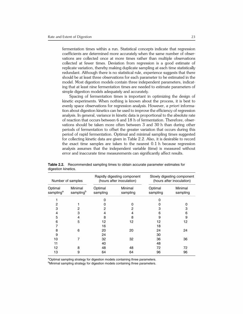
Spacing of fermentation times is important in optimizing the design ofkinetic experiments. When nothing is known about the process, it is best toevenly space observations for regression analysis. However, a priori informa-tion about digestion kinetics can be used to improve the efficiency of regressionanalysis. In general, variance in kinetic data is proportional to the absolute rateof reaction that occurs between 6 and 18 h of fermentation. Therefore, obser-vations should be taken more often between 3 and 30 h than during otherperiods of fermentation to offset the greater variation that occurs during thisperiod of rapid fermentation. Optimal and minimal sampling times suggestedfor collecting kinetic data are given in Table 2.2. Also, it is desirable to recordthe exact time samples are taken to the nearest 0.1 h because regressionanalysis assumes that the independent variable (time) is measured withouterror and inaccurate time measurements can significantly affect results.

Table 2.2. Recommended sampling times to obtain accurate parameter estimates fordigestion kinetics.

Number of samplesRapidly digesting component

(hours after inoculation)Slowly digesting component(hours after inoculation)

Optimalsamplinga

Minimalsamplingb

Optimalsampling

Minimalsampling

Optimalsampling

Minimalsampling

1 0 02 1 0 0 0 03 2 2 2 3 34 3 4 4 6 65 4 8 8 9 96 5 12 12 12 127 16 188 6 20 20 24 249 24 30

10 7 32 32 36 3611 40 4812 8 48 48 72 7213 9 64 64 96 96

aOptimal sampling strategy for digestion models containing three parameters.bMinimal sampling strategy for digestion models containing three parameters.


Observations at the beginning and end of fermentation also are criticalbecause they establish initial solubilization/lag and potential extent of digestion,respectively. Accurate zero-time measurement is needed to distinguish solubil-ization from digestion and estimate the lag effect. Thus, it is important to makeextra observations during the lag phenomenon and to duplicate measurementswhen time equals zero. Replicated measurements are also valuable in estimat-ing the potential extent of digestion.

Models of Digestion

The mathematics for describing first-order dynamic systems is rather simple.Too often it is assumed that rigorous mathematical training is required to modela biological system. Typically, biological conceptualization of the system is themost difficult part of the modelling process. Fear of mathematics has createdtoo much dependence on the selection of equations from those reported in theliterature and has inhibited many scientists from formally describing theirconceptual model in precise mathematical terms that accurately describe thebiological process being investigated. The focus of this section will be thedevelopment of simple models that demonstrate the principles of relatingbiology to the mathematical model and thereby stimulate the reader to generateother suitable models for describing kinetic data.

First-order digestion models can be classified into four types, depending onthe number of compartments and the number and type of reactions (Fig. 2.1).In simultaneous systems, flows from compartments occur simultaneously andindependently. In sequential systems, flow from some compartments becomes

Single compartmentSingle reaction

A . ka

Single compartmentMultiple simultaneous reactions

A . k 1

A . k2

A A

A . kaA

Multiple compartmentsSingle simultaneous reactions

B . kbB

Multiple compartmentsSingle sequential reactions

A . kaA

B . kbB

Fig. 2.1. Illustrations of the various types of first-order models used to describe digestion.

24 D.R. Mertens

the input to other compartments, which creates a ‘time dependency’ for thesecond compartment. Because the models are first-order, they will have anexponential function in the equation for each compartment in the system. Eachtype of model has a distinct set of linear and semi-logarithmic plots of theirdifferential and integral functions that can be used to identify the type ofdigestive process being investigated.

Comments about rates of digestion first appeared in the literature in the1950s, but development of digestion kinetics was hampered by the lack of abiological concept of the digestion process that could be described by a math-ematical formula. Description of the process was difficult because digestioncurveswerenon-linear, differed in asymptote anddid not appear to fit the kineticsof typical chemical reactions. Waldo (1970) was the first to suggest a conceptualbreakthrough that serves as the basis for our current viewof digestion kinetics.Hesuggested that digestion curves are combinations of digestible and indigestiblematerial.His hypothesis that somematter is indigestiblewas based on thework ofWilkins (1969) who observed that some cellulose was undigested in the rumenafter 7 days. Waldo speculated that if the indigestible residue was subtracted, thepotentially digestible fractionmight follow first-order,mass-action kinetics. Inter-estingly, nutritionists would have arrived at this same conclusion if they had usedclassical curve peeling approaches to analyse and interpret digestion curves inwhich fermentation was extended to more than 72 h.

Model 1: Simple first-order digestion with an indigestible fraction

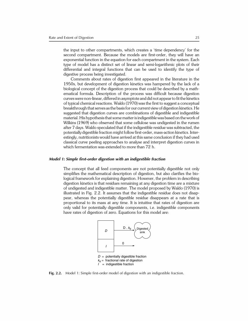
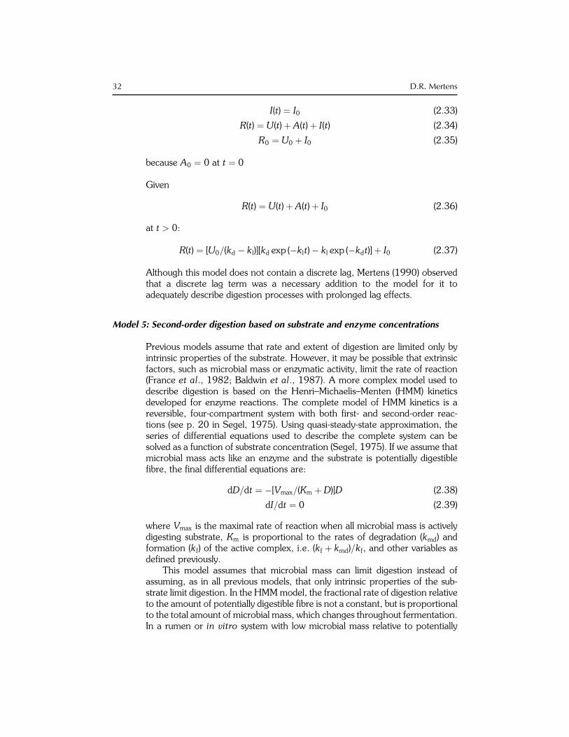
The concept that all feed components are not potentially digestible not onlysimplifies the mathematical description of digestion, but also clarifies the bio-logical framework for explaining digestion. However, the problem in describingdigestion kinetics is that residues remaining at any digestion time are a mixtureof undigested and indigestible matter. The model proposed by Waldo (1970) isillustrated in Fig. 2.2. It assumes that the indigestible residue does not disap-pear, whereas the potentially digestible residue disappears at a rate that isproportional to its mass at any time. It is intuitive that rates of digestion areonly valid for potentially digestible components, i.e. indigestible componentshave rates of digestion of zero. Equations for this model are:

D . kdD

D = potentially digestible fractionkd = fractional rate of digestionI = indigestible fraction

0I

Digestedsink

Fig. 2.2. Model 1: Simple first-order model of digestion with an indigestible fraction.


dD=dt ¼ �kdD (2:1)

dI=dt ¼ 0 (2:2)

where t represents time, I the indigestible residue, D the potentially digestibleresidue and kd the fractional rate constant of digestion.

Although derivatives of time describe the system elegantly, we seldommeasure fluxes under steady-state conditions, instead we measure amounts orconcentrations in a system at specified times. Thus, to describe the data usuallycollected, the above equations must be integrated over time to derive equationsthat correspond to observed data. The integrated equations are:

D(t) ¼ Di exp (�kdt) (2:3)

I(t) ¼ I0 (2:4)

R(t) ¼ D(t)þ I(t) ¼ Di exp (�kdt)þ I0 (2:5)

where I0 and Di are the indigestible and potentially digestible residues at t ¼ 0and R(t) is the total undigested residue at any time.

The implicit assumptions of this first-order model are:

1. The potentially digestible and indigestible pools act as distinct compart-ments with homogeneous kinetic characteristics.2. The fractional rate of digestion is constant and is an intrinsic function ofthe digestive system and the substrate.3. Digestion begins instantly at time zero and continues indefinitely.4. Enzyme or microbial concentrations are not limiting.5. Flux or absolute rate is strictly a function of the amount of potentiallydigestible substrate present at any time.

The equation for D(t) can be transformed into a linear function by naturallogarithmic transformation (ln) and substitution:

ln [D(t)] ¼ ln [Di]� kdt (2:6)

D(t) ¼ R(t)� I0 (2:7)

ln [R(t)� I0] ¼ ln [Di]� kdt (2:8)

By estimating I0 using long-term fermentations and regressing ln [R(t)� I0] ontime, the intercept can be used to estimate Di and the slope or regressioncoefficient estimates the fractional rate constant of digestion (kd), which isdescribed on page 42. The true indigestible fraction can be reached only afterinfinite time, and any fermentation end-point is an overestimation of the trueasymptote. A practical estimate of the asymptote (I0) can be obtained whendigestion is >99% complete. The time at which a pool declines to 1% of itsoriginal value can be approximated by dividing 4.6 by the fractional rate of thepool. For a rate of 0.10/h it will take 46 h to decline to 1% of its original valuecompared with 92 h for a fractional rate of 0.05/h.

Van Milgen et al. (1992) observed differences in the indigestible acid deter-gent fibre fraction when measured after 42 days in situ when host animals were

26 D.R. Mertens

fed diets differing in the proportion of concentrate. They concluded that theindigestible fraction is not an intrinsic characteristic of the feed because it wasaffected by the diet of the animal. However, it could be argued that the intrinsicindigestibility of a feed can only be measured under optimal ruminal conditionsthat result in maximal digestion. Any perturbation of fermentation that does notallow maximal digestion results in indigestible residues that are contaminated byundigested potentially digestible matter. Although indigestibility may not be aconstant intrinsic characteristic of the feed, it may be more appropriate tomeasure the intrinsic indigestibility of the feed using an optimal system andthen modelling the extrinsic factors that cause incomplete digestion, even afterlong fermentation times, as a function of the fermentation system.

The classical test for the appropriateness of the first-order mass-actionmodel is to plot the natural logarithm of the potentially digestible residue versustime. If the plot is linear, the flux or absolute rate of reaction is constant andproportional to the amount of the potentially digestible pool; therefore the first-order, fractional rate constant model is a plausible description of the digestiveprocess. Although most researchers have used R2 to assess linearity, the mostpowerful statistical test is a lack-of-fit test comparing linear and quadraticfunctions of time using multiple samples each measured once in replicatedin vitro or in situ trials. Several scientists (Gill et al., 1969; Smith et al.,1972; Lechtenberg et al., 1974) evaluated the first-order model for potentiallydigestible matter, using either 48- or 72-h fermentations as the end-point forestimating I0. Their results indicated that first-order, mass-action kineticswith an indigestible fraction was an acceptable model of digestion for neutraldetergent fibre (NDF) and cellulose.

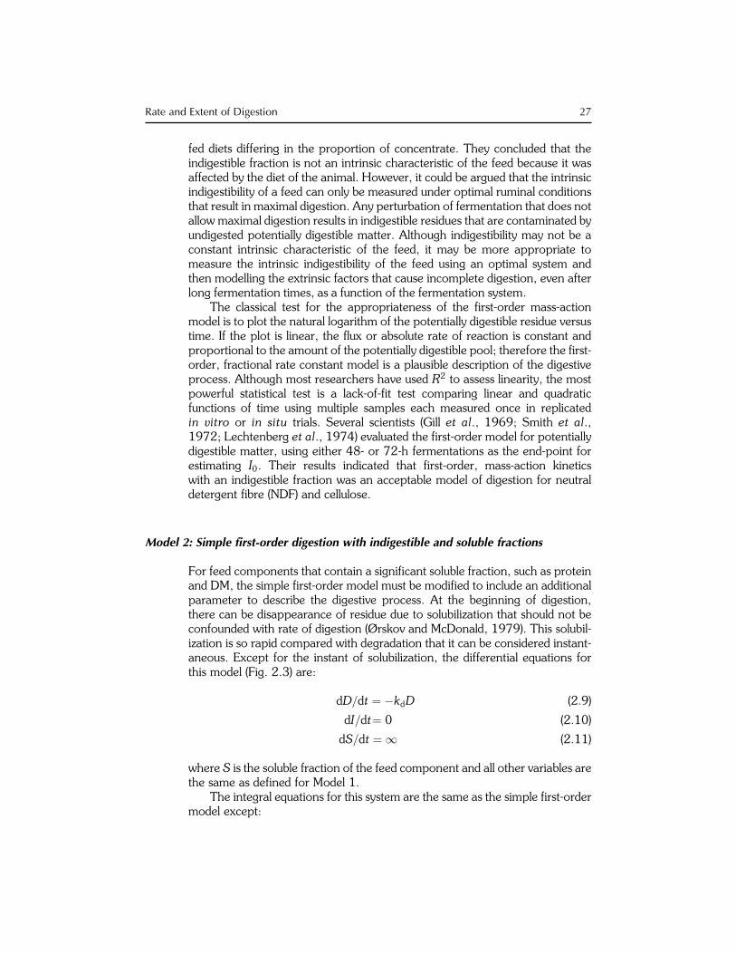
Model 2: Simple first-order digestion with indigestible and soluble fractions

For feed components that contain a significant soluble fraction, such as proteinand DM, the simple first-order model must be modified to include an additionalparameter to describe the digestive process. At the beginning of digestion,there can be disappearance of residue due to solubilization that should not beconfounded with rate of digestion (Ørskov and McDonald, 1979). This solubil-ization is so rapid compared with degradation that it can be considered instant-aneous. Except for the instant of solubilization, the differential equations forthis model (Fig. 2.3) are:

dD=dt ¼ �kdD (2:9)

dI=dt¼ 0 (2:10)

dS=dt ¼ 1 (2:11)

where S is the soluble fraction of the feed component and all other variables arethe same as defined for Model 1.

The integral equations for this system are the same as the simple first-ordermodel except:


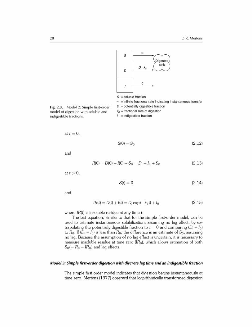
at t ¼ 0,

S(0) ¼ S0 (2:12)

and

R(0) ¼ D(0)þ I(0)þ S0 ¼ Di þ I0 þ S0 (2:13)

at t > 0,

S(t) ¼ 0 (2:14)

and

IR(t) ¼ D(t)þ I(t) ¼ Di exp (�kdt)þ I0 (2:15)

where IR(t) is insoluble residue at any time t.The last equation, similar to that for the simple first-order model, can be

used to estimate instantaneous solubilization, assuming no lag effect, by ex-trapolating the potentially digestible fraction to t ¼ 0 and comparing (Di þ I0)to R0. If (Di þ I0) is less than R0, the difference is an estimate of S0, assumingno lag. Because the assumption of no lag effect is uncertain, it is necessary tomeasure insoluble residue at time zero (IR0), which allows estimation of bothS0ð¼ R0 � IR0Þ and lag effects.

Model 3: Simple first-order digestion with discrete lag time and an indigestible fraction

The simple first-order model indicates that digestion begins instantaneously attime zero. Mertens (1977) observed that logarithmically transformed digestion

Fig. 2.3. Model 2: Simple first-ordermodel of digestion with soluble andindigestible fractions.

D . kdD

S = soluble fraction� = infinite fractional rate indicating instantaneous transferD = potentially digestible fractionkd = fractional rate of digestionI = indigestible fraction

0I

�S

Digestedsink

28 D.R. Mertens

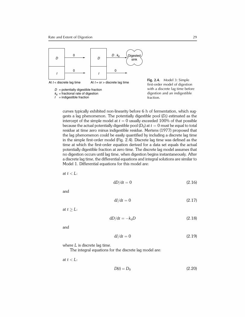
curves typically exhibited non-linearity before 6 h of fermentation, which sug-gests a lag phenomenon. The potentially digestible pool (Di) estimated as theintercept of the simple model at t ¼ 0 usually exceeded 100% of that possiblebecause the actual potentially digestible pool (D0) at t ¼ 0 must be equal to totalresidue at time zero minus indigestible residue. Mertens (1977) proposed thatthe lag phenomenon could be easily quantified by including a discrete lag timein the simple first-order model (Fig. 2.4). Discrete lag time was defined as thetime at which the first-order equation derived for a data set equals the actualpotentially digestible fraction at zero time. The discrete lag model assumes thatno digestion occurs until lag time, when digestion begins instantaneously. Aftera discrete lag time, the differential equations and integral solutions are similar toModel 1. Differential equations for this model are:

at t < L:

dD=dt ¼ 0 (2:16)

and

dI=dt ¼ 0 (2:17)

at t � L:

dD=dt ¼ �kdD (2:18)

and

dI=dt ¼ 0 (2:19)

where L is discrete lag time.The integral equations for the discrete lag model are:

at t < L:

D(t) ¼ D0 (2:20)

D . kdD

D = potentially digestible fractionkd = fractional rate of digestionI = indigestible fraction

0I

0D

0I

At t < discrete lag time At t = or > discrete lag time

Digestedsink

Fig. 2.4. Model 3: Simplefirst-order model of digestionwith a discrete lag time beforedigestion and an indigestiblefraction.


and

I(t) ¼ I0 (2:21)

R(t) ¼ D0 þ I0 (2:22)

at t � L:

D(t) ¼ Di exp (�kd[t� L]) (2:23)

and

I(t) ¼ I0 (2:24)

and

R(t) ¼ D(t)þ I(t) ¼ Di exp (�kd[t� L])þ I0 (2:25)

At t ¼ L:

R0 � I0 ¼ D0 ¼ Di exp (�kd[L]) (2:26)

and

L ¼ [ ln (D0)� ln (Di)]=(�kd) (2:27)

This model can be modified easily to incorporate the digestion kinetics of feedcomponents that exhibit initial solubilization (Dhanoa, 1988). However, toestimate lag time for these components, there must be a measure of the amountof insoluble residue at t ¼ 0 to provide an estimate of IR0 that must equal(D0 þ I0). Although the discrete lag model may not adequately describe lagphenomena for use in dynamic simulation models, it provides a simple andquantitative measure of the lag effect that can be used to compare feeds.Although Lopez et al. (1999) concluded that discrete lag models are difficultto justify biologically because some digestion occurs before lag time, theyobserved that the simple exponential model with discrete lag was only rankedbelow generalized exponential and inverse polynomial models for lack-of-fit,rank of residual mean of squares (RMS) and average RMS when used to describein situ DM, NDF and protein degradation. However, generalized exponentialand inverse polynomial models also have difficult biological interpretations.

When the intercept (Di) is greater than D0 clearly some type of lag phe-nomenon has occurred (see Fig. 2.9 in the Curve Peeling section). WhenDi < D0, the discrete lag time L is negative, which implies that digestion beginsbefore t ¼ 0, a result that is difficult, if not impossible, to accept biologically.However, there is a biological explanation for negative lag times because theysimply indicate that instantaneous solubilization has occurred, which equalsD0 �Di. However, both solubilization and lag can occur when initial solubiliza-tion is greater than that indicated by the difference betweenD0 andDi, but theireffects cannot be separated unless IR0 is measured at time zero so that D0 canbe estimated. Setting bounds on discrete lag to prevent it from being less thanzero is not appropriate because it eliminates the possibility for detecting solu-bilization and can result in biased estimates of kinetic parameters.

30 D.R. Mertens

Model 4: Sequential first-order reaction for lag and digestion with an indigestiblefraction

Other models of digestion have been proposed that describe digestion as asequential compartmental process (Allen and Mertens, 1988; Mertens, 1990;Van Milgen et al., 1991). In these models, the digestive process is described bya two-step mechanism (Fig. 2.5). In the first stage, lag is modelled as a first-order process involving the change in the substrate from an unavailable form toone that is available for digestion. Biologically, this step could represent hydra-tion of substrate, removal of digestion inhibitors, or attachment or close asso-ciation of microorganisms with the substrate. The second stage is also first-order and represents actual degradation of the substrate. This model exhibits asmooth curvilinear transition from no digestion at t ¼ 0 to maximum absolutedigestion rate at the inflection point of the digestion curve. Differential equa-tions for this model are:

dU=dt ¼ �klU (2:28)

dA=dt ¼ klU � kdA (2:29)

dI=dt ¼ 0 (2:30)

where U is the unavailable potentially digestible pool, A is the potentiallydigestible pool that is available for digestion, I is the indigestible residue, kl isthe fractional rate constant for lag and kd is the fractional rate constant fordigestion.

The integral equations for this digestive process are:

U(t) ¼ U0 exp (�klt) (2:31)

A(t) ¼ U0[kl=(kd � kl)][ exp (�klt)� exp (�kdt)] (2:32)

A

U = unavailable potentially digestible fractionk l = fractional rate of availability (lag phenomena)A = available potentially digestible fractionkd = fractional rate of digestionI = indigestible fraction

U . k l A . kdU

0I

Digestedsink

Fig. 2.5. Model 4: Sequential multi-compartmental model of digestion and lag with anindigestible fraction.


I(t) ¼ I0 (2:33)

R(t) ¼ U(t)þA(t)þ I(t) (2:34)

R0 ¼ U0 þ I0 (2:35)

because A0 ¼ 0 at t ¼ 0

Given

R(t) ¼ U(t)þ A(t)þ I0 (2:36)

at t > 0:

R(t) ¼ [U0=(kd � kl)][kd exp (�klt)� kl exp (�kdt)]þ I0 (2:37)

Although this model does not contain a discrete lag, Mertens (1990) observedthat a discrete lag term was a necessary addition to the model for it toadequately describe digestion processes with prolonged lag effects.

Model 5: Second-order digestion based on substrate and enzyme concentrations

Previous models assume that rate and extent of digestion are limited only byintrinsic properties of the substrate. However, it may be possible that extrinsicfactors, such as microbial mass or enzymatic activity, limit the rate of reaction(France et al., 1982; Baldwin et al., 1987). A more complex model used todescribe digestion is based on the Henri–Michaelis–Menten (HMM) kineticsdeveloped for enzyme reactions. The complete model of HMM kinetics is areversible, four-compartment system with both first- and second-order reac-tions (see p. 20 in Segel, 1975). Using quasi-steady-state approximation, theseries of differential equations used to describe the complete system can besolved as a function of substrate concentration (Segel, 1975). If we assume thatmicrobial mass acts like an enzyme and the substrate is potentially digestiblefibre, the final differential equations are:

dD=dt ¼ �[Vmax=(Km þD)]D (2:38)

dI=dt ¼ 0 (2:39)

where Vmax is the maximal rate of reaction when all microbial mass is activelydigesting substrate, Km is proportional to the rates of degradation (kmd) andformation (kf) of the active complex, i.e. (kf þ kmd)=kf, and other variables asdefined previously.

This model assumes that microbial mass can limit digestion instead ofassuming, as in all previous models, that only intrinsic properties of the sub-strate limit digestion. In the HMMmodel, the fractional rate of digestion relativeto the amount of potentially digestible fibre is not a constant, but is proportionalto the total amount of microbial mass, which changes throughout fermentation.In a rumen or in vitro system with low microbial mass relative to potentially

32 D.R. Mertens

digestible sites, the order of the overall reaction varies with respect to theconcentration of the substrate. Initially, the concentration of substrate is highrelative to microbial mass (D � Km) and dD=dt ¼ �Vmaxt, which is zero-orderrelative to D. This occurs because at high substrate concentrations, the absoluterate of reaction is more a function of the amount of microbial mass than ofsubstrate concentration. As potentially digestible substrate is degraded, itsconcentration decreases relative to microbial mass (D � Km) and dD=dt ¼�(Vmax=Km)D, i.e. the reaction is first-order with respect to D with a fractionalrate equal to (Vmax=Km).

The HMM-type differential equation can be integrated (Segel, 1975) to:

Vmaxt ¼ �Km ln (D=D0)� (D�D0) (2:40)

Although this equation cannot be solved analytically for D at any time, even ifVmax and Km are known, it can be rearranged to a linear form and used toestimate Vmax and Km from time-series measurements. A linear form of theintegral equation that is useful is:

(D0 �D)=t ¼ �Km[ ln (D0=D)=t]þ Vmax (2:41)

By regressing (D0 ---D)=t versus ln (D0=D)=t, Km and Vmax can be estimatedfrom the slope and intercept, respectively. To obtain accurate estimates ofparameters, the values of D should vary from approximately 0:1Km to 10Km.

After estimates of Km and Vmax are determined, the differential form of theHMM-type equation can be integrated numerically to obtain values ofD(t) at anytime. Use of numerical integration is only a minor inconvenience with theavailability of computers and computer programs. A factor complicating theuse of HMM kinetics with microbial systems is that microbial activity increasesduring the reaction asmicrobes use substrate for growth. Thus, microbial activityis not constant in a fermentation system like enzyme concentrations are inclassical enzyme kinetics. To more accurately mimic HMM kinetics, microbialgrowth could be inhibited during kinetic measurements or the model could bemodified to add microbial growth and then derive a new equation that moreaccurately describesmicrobial fermentation of a substrate. Biologically theHMMmodel is valid only if microbial concentrations limit degradation during the earlyperiod of fermentation. Thus, one can never be sure when interpreting HMMresults that intrinsic limitations of the substrate are being evaluated becauseVmax

depends on microbial concentration, and the intrinsic second-order rate con-stant of substrate disappearance is not estimated.

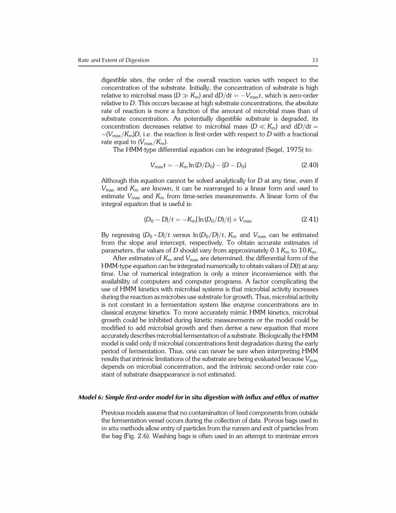
Model 6: Simple first-order model for in situ digestion with influx and efflux of matter

Previous models assume that no contamination of feed components from outsidethe fermentation vessel occurs during the collection of data. Porous bags used inin situmethods allow entry of particles from the rumen and exit of particles fromthe bag (Fig. 2.6). Washing bags is often used in an attempt to minimize errors


associated with the former problem, whereas grinding samples coarsely is some-times used to minimize the latter. However, washing bags varies substantiallyamong laboratories and it is difficult, if not impossible, to balance the errorsbetween washing out contaminating matter and removing actual sample. Coarsegrinding may influence digestion processes and alter digestion kinetics (Michalet-Doreau and Cerneau, 1991). Because neither of these strategies may solve theproblems associated with measurement of digestion kinetics in situ, it is intuitivethatmodels used for in vitro digestion kinetics may not be valid for in situ kinetics.

In this model (Fig. 2.6), the number of fine digestible and indigestibleparticles in the feed and the amount of fine digestible particles in the rumenare assumed to be negligible. Thus, influx and efflux of fine particles is assumedto be only indigestible fibre from ruminal contents. The influx rate is assumed tobe zero-order, i.e. is only a function of time, and is probably related to pore sizeand surface area of bag material. Differential equations describing the digestionof fibre in situ are:

dD=dt ¼ �kdD (2:42)

dI=dt ¼ 0 (2:43)

dIe=dt ¼ fi � keIe (2:44)

where Ie is the pool of escapable indigestible particles from the rumen that arein the bag, fi is the zero-order influx rate of particles into the bag and ke is thefirst-order efflux rate of fine, escapable particles from the bag.

The integrated solutions to these equations are:

D(t) ¼ D0 exp (�kdt) (2:45)

I(t) ¼ I0 (2:46)

Ie(t) ¼ (fi=ke)[1� exp (�ket)] (2:47)

Fig. 2.6. Model 6: Simple first-ordermodel of digestion with an indigestiblefraction and influx and efflux ofindigestible fine particles in the rumenthat can occur when using an in situsystem.

D . kdD

D = potentially digestible fractionkd = fractional rate of digestionI = indigestible fractionIe = exogenous indigestible fine particlesf i = zero-order influx rate of exogenous fine particleske = fractional rate of escape of fine particles

Ie . keIe

0I

fi

Digestedsink

Ruminalparticle

sink

Ruminalparticle

sink

34 D.R. Mertens

The total residue in the bag at any time t is:

R(t) ¼ D(t)þ I(t)þ Ie(t) (2:48)

R(t) ¼ D0 exp (�kdt)þ I0 þ (fi=ke)[1� exp (�ket)] (2:49)

Because the influx rate is zero-order and has the units mass per unit of time, theresidue at any time must be expressed in the same units to estimate theparameters of this model using non-linear regression. Thus R(t) cannot beexpressed as a percentage of the starting sample weight, but must be expressedas mg, g, etc. This differs from first-order Models 1 to 4 that obtain the samefractional rate constants irrespective of the units used to express R(t).

If it is postulated that washing fine particles out of bags follows first-orderkinetics (the amount washed out at any time t is proportional to the amountof fine particles in the bag at any time [Ie(t)]) and the concentration of fineparticles in the wash water is so small that influx during washing is negligible, itcan be shown that changes during washing are described by the followingequations:

dD=d(tw) ¼ 0 (2:50)

dI=d(tw) ¼ 0 (2:51)

dIe=d(tw) ¼ �kwIe (2:52)

where tw is washing time and kw is the fractional washout rate of fine particlesfrom the in situ bag.

Because the amount of each pool at the time of washing is equal to D(t), I(t)and Ie(t), respectively, it can be shown that after any washing time tw:

R(t) ¼ D(t)þ I(t)þ Ie(t) exp (� kwtw) (2:53)

R(t) ¼ D0 exp (�kdt)þ I0 þ [ exp (�kwtw)](fi=ke)[1� exp (�ket)] (2:54)

If washing time tw is the same for all samples, the term exp (�kwtw) becomes aconstant, and when non-linear least squares regression is used to estimate theparameters of the model the term [ exp (�ketw)](fi=ke) will be determined as asingle coefficient.

The equation for Model 6 is similar to the simple equation for an in vitrosystem (Model 1) except that an additional term is needed to describe the netaccumulation of fine particles in the bag at any time t. Model 6 predicts thatinfiltration of fine particles will increase to an asymptote that is equal to theratio of influx and efflux rates. This indicates that indigestibility will be overesti-mated in situ and suggests that fractional rates and lag times will be biased ifsimpler models such as Models 1 to 4 are used that do not contain terms for netaccumulation of residue in the bag and washing does not remove all influxmaterial.

Analysing models derived from the biology of the specific digestion processdemonstrates one of the often overlooked uses of models. Once equations arederived, they can be used to detect differences in timing and magnitude


between alternative models and suggest experimental designs that can be usedto effectively compare them. Model 6 could be modified to incorporate add-itional biological processes including losses of fine particles in a more finelyground sample than is assumed in Model 6 or by including a discrete lag timeduring which influx and efflux occurred, but digestion did not. However, thesemodels require additional terms that cannot be estimated realistically usingcurrent data collection and fitting techniques.

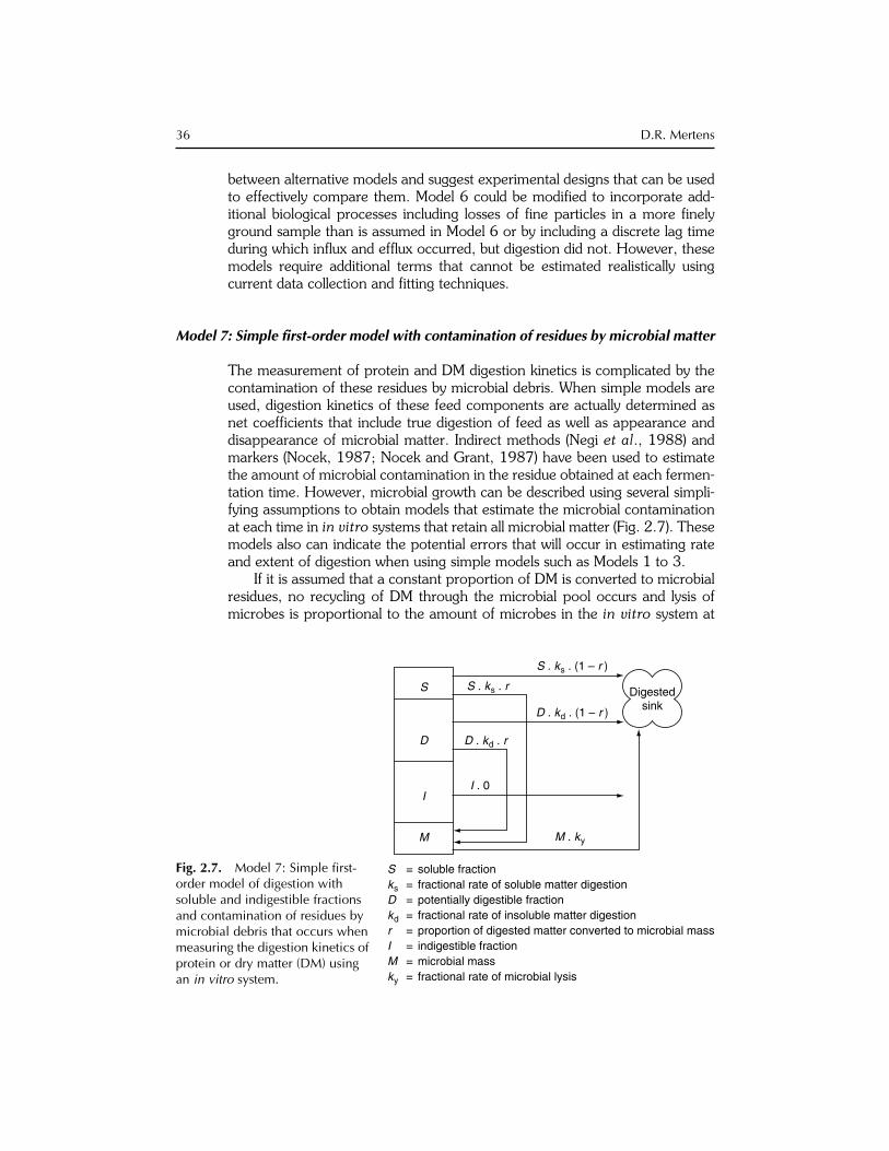
Model 7: Simple first-order model with contamination of residues by microbial matter

The measurement of protein and DM digestion kinetics is complicated by thecontamination of these residues by microbial debris. When simple models areused, digestion kinetics of these feed components are actually determined asnet coefficients that include true digestion of feed as well as appearance anddisappearance of microbial matter. Indirect methods (Negi et al., 1988) andmarkers (Nocek, 1987; Nocek and Grant, 1987) have been used to estimatethe amount of microbial contamination in the residue obtained at each fermen-tation time. However, microbial growth can be described using several simpli-fying assumptions to obtain models that estimate the microbial contaminationat each time in in vitro systems that retain all microbial matter (Fig. 2.7). Thesemodels also can indicate the potential errors that will occur in estimating rateand extent of digestion when using simple models such as Models 1 to 3.

If it is assumed that a constant proportion of DM is converted to microbialresidues, no recycling of DM through the microbial pool occurs and lysis ofmicrobes is proportional to the amount of microbes in the in vitro system at

Fig. 2.7. Model 7: Simple first-order model of digestion withsoluble and indigestible fractionsand contamination of residues bymicrobial debris that occurs whenmeasuring the digestion kinetics ofprotein or dry matter (DM) usingan in vitro system.

D

S = soluble fractionks = fractional rate of soluble matter digestionD = potentially digestible fractionkd = fractional rate of insoluble matter digestionr = proportion of digested matter converted to microbial massI = indigestible fractionM = microbial massky = fractional rate of microbial lysis

I

S . ks . r

D . kd . r

I . 0

S

D . kd . (1 – r )

S . ks . (1 – r )

M . kyM

Digestedsink

36 D.R. Mertens

any time, the following differential equations can be used to describe thedigestion of DM:

dS=dt ¼ �rksS� (1� r)ksS ¼ �ksS (2:55)

dD=dt ¼ �rkdD� (1� r)kdD ¼ �kdD (2:56)

dI=dt ¼ 0 (2:57)

dM=dt ¼ rksSþ rkdD� kyM (2:58)

where r is the proportion of digested matter that is converted to microbial DM,ks is the fractional rate of digestion of soluble matter, ky is the fractional lysisrate of microbial DM, M is the pool of microbial matter in the in vitro vessel atany time and all other variables are defined as for Model 2. In this model,digestion of soluble matter is not assumed to be instantaneous, although thisassumption could have been used.

The differential equations can be integrated to obtain the following solutions:

S(t) ¼ S0 exp (�kst) (2:59)

D(t) ¼ D0 exp (�kdt) (2:60)

I(t) ¼ I0 (2:61)

M(t) ¼ [rksS0=(ky � ks)][ exp (�kst)� exp (�kyt)]

þ [rkdD0=(ky � kd)][ exp (�kdt)� exp (�kyt)](2:62)

To solve for M(t), it was assumed that a blank microbial residue was subtractedso that M ¼ 0 at time ¼ 0. If residues are filtered to isolate undigested DMresidues, S(t) will not be measured at any time. Since R0 ¼ S0 þD0 þ I0, thefunction (R0 �D0 � I0) can be substituted into the microbial contaminationfunction to eliminate the S0 term. The final DM residue function is:

DM(t) ¼ D0 exp (�kdt)þ I0 þ [rks(R0 �D0 � I0)=(ky � ks)][ exp (�kst)

� exp (�kyt)]þ [rkdD0=(ky � kd)][ exp (�kdt)� exp (�kyt)](2:63)

Model 7 could be simplified to assume an instantaneous loss of solublematter and conversion to microbial mass, or it could be made more complex byincluding recycling of microbial DM and addition of lag phenomena. However,the biological process described for Model 7 and the equations that areobtained can be used to demonstrate the errors inherent in using simple modelssuch as Models 1 to 3 to describe a complex process involving microbial growthwhen microbial debris contaminates the feed component that is being studied.The equation used to describe Model 7, which includes microbial lysis, indicatesthat microbial debris increases, then decreases, during fermentation whichagrees with data of Nocek (1987). Observations by Negi et al. (1988) indicatethat microbial nitrogen contamination increased to an asymptote during fer-mentation; this occurrence could be modelled by assuming that no lysis occurs.Both Nocek (1987) and Negi et al. (1988) used an in situ procedure to


determine digestion kinetics and additional terms would be needed to describethe influx and efflux of microbial debris that does not occur in the in vitrosystem described by Model 7.

If Model 7 is simulated assuming no lag and the resulting data are fitted toModel 2, two principles can be demonstrated. First, apparent or net fractionalrates of digestion are biased estimates of the true fractional digestion rates ofthe feed. Second, the standard technique for assessing the adequacy of the first-order model of digestion is not sensitive enough to detect model discrepanciesassociated with production or recycling of microbial mass. The standard test fordetermining the adequacy of the first-order model is to determine the R2, i.e.R2 near 1.00 are assumed to indicate a good fit of the data to the first-ordermodel. However, it is possible to obtain R2 greater than 0.9 for residuescontaminated with microbial debris, suggesting the simple first-order model isa good fit to the data. Although R2 can be criticized as a test of model adequacy,even lack-of-fit tests may not detect inadequate models with typical biologicalvariation. Parameters will be biased when a simple model is used to estimatedigestion kinetics for components contaminated with microbial debris and itappears that biological justification rather than statistical evaluation is the key todetermining the validity of models for use in estimating digestion kinetics.

Fitting Digestion Data to Kinetic Models

Curve peeling

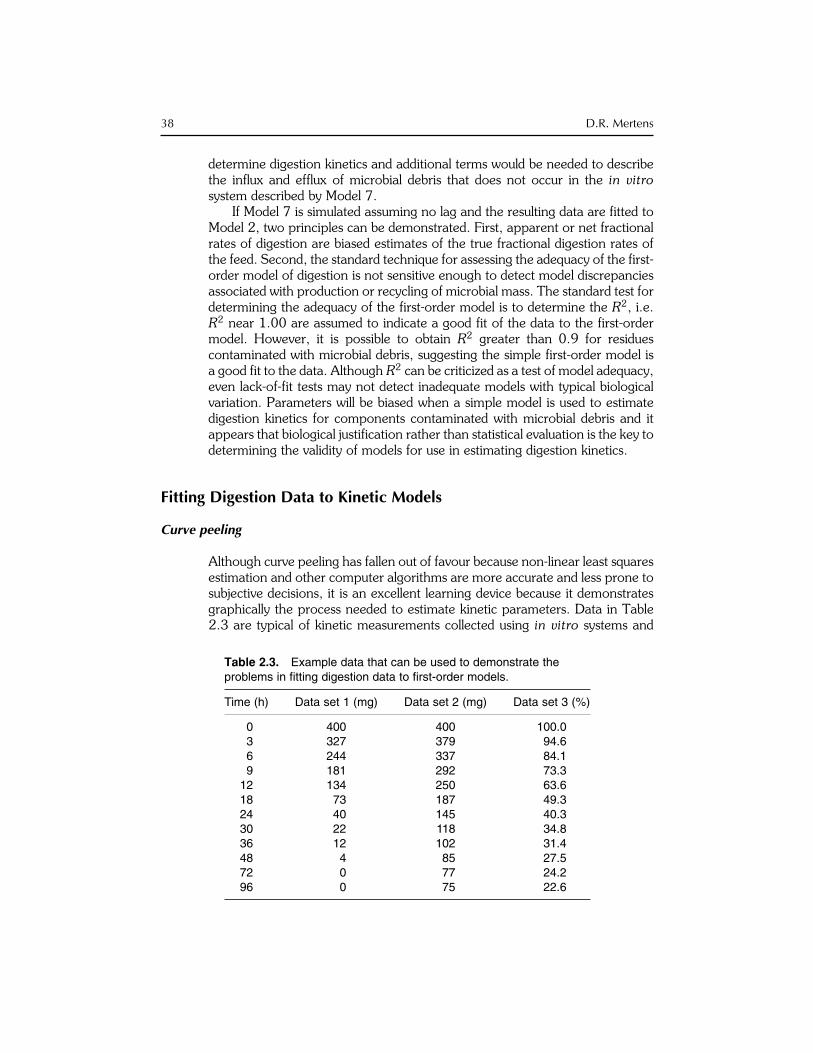
Although curve peeling has fallen out of favour because non-linear least squaresestimation and other computer algorithms are more accurate and less prone tosubjective decisions, it is an excellent learning device because it demonstratesgraphically the process needed to estimate kinetic parameters. Data in Table2.3 are typical of kinetic measurements collected using in vitro systems and

Table 2.3. Example data that can be used to demonstrate theproblems in fitting digestion data to first-order models.

Time (h) Data set 1 (mg) Data set 2 (mg) Data set 3 (%)

0 400 400 100.03 327 379 94.66 244 337 84.19 181 292 73.3

12 134 250 63.618 73 187 49.324 40 145 40.330 22 118 34.836 12 102 31.448 4 85 27.572 0 77 24.296 0 75 22.6

38 D.R. Mertens

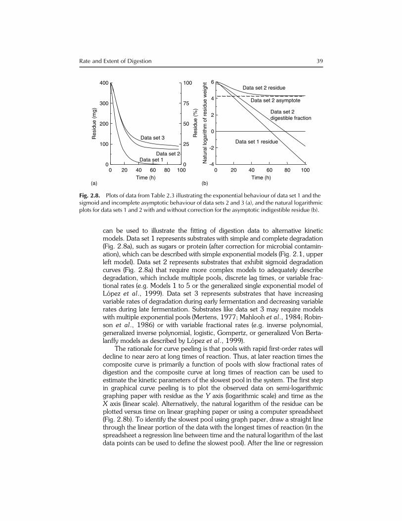
can be used to illustrate the fitting of digestion data to alternative kineticmodels. Data set 1 represents substrates with simple and complete degradation(Fig. 2.8a), such as sugars or protein (after correction for microbial contamin-ation), which can be described with simple exponential models (Fig. 2.1, upperleft model). Data set 2 represents substrates that exhibit sigmoid degradationcurves (Fig. 2.8a) that require more complex models to adequately describedegradation, which include multiple pools, discrete lag times, or variable frac-tional rates (e.g. Models 1 to 5 or the generalized single exponential model ofLopez et al., 1999). Data set 3 represents substrates that have increasingvariable rates of degradation during early fermentation and decreasing variablerates during late fermentation. Substrates like data set 3 may require modelswith multiple exponential pools (Mertens, 1977; Mahlooh et al., 1984; Robin-son et al., 1986) or with variable fractional rates (e.g. inverse polynomial,generalized inverse polynomial, logistic, Gompertz, or generalized Von Berta-lanffy models as described by Lopez et al., 1999).

The rationale for curve peeling is that pools with rapid first-order rates willdecline to near zero at long times of reaction. Thus, at later reaction times thecomposite curve is primarily a function of pools with slow fractional rates ofdigestion and the composite curve at long times of reaction can be used toestimate the kinetic parameters of the slowest pool in the system. The first stepin graphical curve peeling is to plot the observed data on semi-logarithmicgraphing paper with residue as the Y axis (logarithmic scale) and time as theX axis (linear scale). Alternatively, the natural logarithm of the residue can beplotted versus time on linear graphing paper or using a computer spreadsheet(Fig. 2.8b). To identify the slowest pool using graph paper, draw a straight linethrough the linear portion of the data with the longest times of reaction (in thespreadsheet a regression line between time and the natural logarithm of the lastdata points can be used to define the slowest pool). After the line or regression

-4

-2

0

2

4

6

Nat

ural

loga

rithm

of r

esid

ue w

eigh

t

Data set 1 residue

Data set 2 residue

Data set 2 asymptote

Data set 2digestible fraction

(b)(a)

0 20 40 60 80 100Time (h)

0 20 40 60 80 100Time (h)

0

100

200

300

400

Res

idue

(m

g)

0

25

50

75

100

Res

idue

(%

)

Data set 1Data set 2

Data set 3

Fig. 2.8. Plots of data from Table 2.3 illustrating the exponential behaviour of data set 1 and thesigmoid and incomplete asymptotic behaviour of data sets 2 and 3 (a), and the natural logarithmicplots for data sets 1 and 2 with and without correction for the asymptotic indigestible residue (b).


is established, it is peeled from the composite curve by subtracting its actualvalue (not its logarithm) at each time from the value of the composite line. Thisleaves a residual line that is the result of other pools in the system. If the residualline is linear, curve peeling is complete; if it is curvilinear, the peeling procedureis repeated on the residual line. The slope of each line is the fractional rateconstant of that pool or compartment, whereas the intercept of each line maybe the size of the pool or may be undefined, depending on whether the systemhas sequentially or simultaneously reacting pools. In practice, it is difficult toseparate more than three pools unless extremely long times of reaction arerecorded and the fractional rates differ greatly. It also is difficult to separatesystems in which the fractional rates do not differ by a factor of three or more.

The plot of data set 1 (Table 2.3) is linear with only a slight deviation duringinitial fermentation (Fig. 2.8b). The linear semi-logarithmic line indicates that afirst-order model with a constant fractional rate (equal to the slope of the line) isplausible and a model like that in Fig. 2.1 (upper left model) could be used todescribe degradation of this substrate. However, data set 2 (Table 2.3) results ina non-linear semi-logarithmic line that appears to be asymptotic (Fig. 2.8b). Anasymptotic plateau indicates a pool with a slope of zero (i.e. an indigestiblepool), which corresponds to an indigestible residue that never degrades in theanaerobic system in which feeds are fermented as indicated by Wilkins (1969).Using curve peeling, the indigestible pool, which is typically assumed to be theresidue after long (> 72h) fermentation times, is subtracted from the compos-ite data line to obtain a residual digestible pool or fraction (Fig. 2.8b). The linefor the digestible fraction is linear suggesting that it can be represented by afirst-order model with a constant fractional rate of digestion except during earlyfermentation.

Because a fractional digestion rate can only apply to a pool that is digest-ible, it is crucial that a valid estimate of the indigestible fraction be used todetermine the potentially digestible fraction by difference. Mertens (1977)illustrated the consequences of using 48, 72, or 96-h fermentations to estimatethe indigestible fibre fraction. If the 48-h observation in data set 3 (Table 2.3) isused to estimate the asymptote of fermentation, the residual plot of the poten-tially digestible fraction will be concave and shifted to the left, resulting in anoverestimation of the indigestible fraction, fractional rate, and discrete lag timecompared with the 72-h fermentation end-point. When data sets terminate at24 or 48 h of fermentation, it is easy to miss the asymptotic nature of thedigestion process in anaerobic systems and conclude that degradation can bedescribed by a single exponential pool without an indigestible fraction. Thisconclusion results in estimates of fractional rates that are low compared withthe true fractional rate of digestion because their rates are ‘averaged’ over bothpotential digestible and indigestible pools. These results not only cause confu-sion in the literature, but also they are fundamentally incorrect because theyviolate two assumptions of kinetic principles. First, the single digestion pool isan aggregate of both digestible and indigestible components and does notrepresent a pool with homogeneous kinetic properties. Second, the inclusionof the indigestible fraction in a digesting compartment results in the paradoxthat indigestible residue has a non-zero fractional rate of digestion.

40 D.R. Mertens

When long times of fermentation (>90h) are used to estimate indigestibleresidues, semi-logarithmic plots may become convex and non-linear suggestingthat the potentially digestible fraction can be described as the sum of two ormore first-order pools with different rates. Robinson et al. (1986) confirmedthat this model is most appropriate in some situations. Mahlooh et al. (1984)carried this approach to its extreme, and proposed that a stochastic modelcould describe digestion that assumes a population of digestible pools with agamma distribution of factional rates. Alternatively, sigmoid mathematicalmodels (inverse polynomial, generalized inverse polynomial, logistic, Gom-pertz, and generalized Von Bertalanffy) as described by Lopez et al. (1999),which have diminishing variable fractional rates toward the end of fermenta-tion, can describe the degradation curve, but these models cannot be parame-terized by curve peeling.

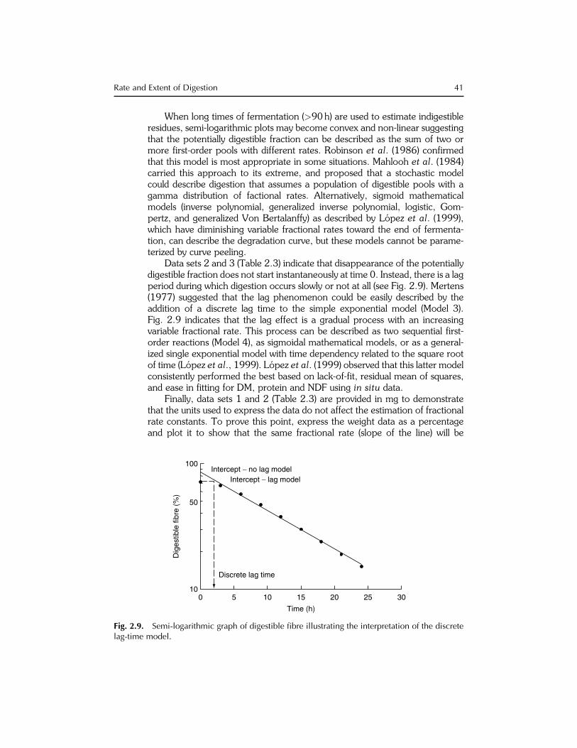
Data sets 2 and 3 (Table 2.3) indicate that disappearance of the potentiallydigestible fraction does not start instantaneously at time 0. Instead, there is a lagperiod during which digestion occurs slowly or not at all (see Fig. 2.9). Mertens(1977) suggested that the lag phenomenon could be easily described by theaddition of a discrete lag time to the simple exponential model (Model 3).Fig. 2.9 indicates that the lag effect is a gradual process with an increasingvariable fractional rate. This process can be described as two sequential first-order reactions (Model 4), as sigmoidal mathematical models, or as a general-ized single exponential model with time dependency related to the square rootof time (Lopez et al., 1999). Lopez et al. (1999) observed that this latter modelconsistently performed the best based on lack-of-fit, residual mean of squares,and ease in fitting for DM, protein and NDF using in situ data.

Finally, data sets 1 and 2 (Table 2.3) are provided in mg to demonstratethat the units used to express the data do not affect the estimation of fractionalrate constants. To prove this point, express the weight data as a percentageand plot it to show that the same fractional rate (slope of the line) will be

0 5 10 15 20 25 30

Time (h)

10

100

Dig

estib

le fi

bre

(%)

Intercept − no lag modelIntercept − lag model

Discrete lag time

50

Fig. 2.9. Semi-logarithmic graph of digestible fibre illustrating the interpretation of the discretelag-time model.


obtained whether the data are expressed as mg or percentages. It is oftenassumed that the data must be expressed as percentages before kinetic analysisbecause fractional rates are sometimes reported in the literature as %/h.The first-order rate constant is a pure fraction that has no units other thanper hour. Expressing fractional rates as percentages or g/kg is confusing anderroneous.

Logarithmic transformation and regression

Although graphical curve peeling visualizes the process, estimating digestionkinetics using linear regression of logarithmically transformed data is a statis-tical adaptation of the process for estimating kinetic parameters. In thismethod, the indigestible residue, typically estimated from the last fermentationpoint, is subtracted from the measured residues at each fermentation time. Thenatural logarithm of the resulting potentially digestible residue is regressed ontime (see Eq. 2.8). The regression coefficient obtained is an estimate of the first-order rate constant of digestion (if logarithms to the base 10 are used theresulting rate must be multiplied by 2.302). The regression intercept can beused to calculate a discrete lag time (Mertens and Loften, 1980) if a measure-ment of residue at t ¼ 0 is available (Eq. 2.27). If a lag effect is detected, thefermentations prior to the lag time must not be included because they biasthe regression and result in an underestimation of both fractional rate anddiscrete lag time. The log-transform regression method, when combined witha good approximation of the indigestible residue and elimination of observa-tions prior to lag, can yield reasonably accurate estimates of kinetic parameters.

An implicit assumption of logarithmic transformation is that the randomerror in the data is multiplicative rather than additive (Mertens and Loften,1980; Moore and Cherney, 1986), which may be a potential problem in theuse of the logarithmic transformation method for estimating kinetic param-eters. In effect, log transformation assumes that observations with smallerresidues (after long times of fermentation) have smaller errors and effectivelygives greater weight to their contribution during regression analysis. However,it is typically observed that variation among replicated measurements is lowestat the end of fermentation when residue amounts are smallest. Therefore, itdoes not seem that the multiplicative error distribution associated with logarith-mic transformation is a significant problem during parameter estimation.

The most serious problem with the logarithmic transformation and linearregression method of estimating kinetic parameters is error in estimating theindigestible fraction. Indigestibility measured at any time other than infinity is anoverestimate of the asymptotic indigestible residue. A more accurate estimateof the indigestible residue can be obtained by iteratively assuming the indigest-ible residue is smaller than the observed end-point of fermentation and recal-culating the log transformed linear regression coefficients. As the estimate ofthe indigestible residue is reduced, the R2 of regression increases until theindigestible residue that optimizes the R2 is obtained. The use of fermentationend-points as approximations of the indigestible residue can result in fractional

42 D.R. Mertens

rates of digestion that are 10% to 15% too high and discrete lag times that are20% to 30% too long.

Non-linear least squares regression

Many problems associated with curve peeling and logarithmic transformation-linear regression can be overcome by estimating kinetic parameters using non-linear least squares regression procedures (Mertens and Loften, 1980; Mooreand Cherney, 1986). As with linear regression, non-linear regression deter-mines the values of regression coefficients that minimize the residual sums ofsquares from regression. Unlike linear regression, non-linear regression cannotcalculate parameter solutions directly. Instead the estimates of model param-eters are adjusted iteratively from an initial estimate to reduce the squareddeviations from regression using numerical or analytical derivatives of thenon-linear model. This approach is similar to that accomplished by manualiteration. Iteration continues until a negligible improvement in fit of the data tothe model occurs. Several algorithms are used for non-linear regression, in-cluding steepest descent, Gauss–Newton, Marquardt compromise and simplex.Each algorithm has advantages and disadvantages that can influence the rateand occurrence of convergence to a solution that minimizes the deviation fromregression to an acceptable level. Regardless of the algorithm used, standarderrors of parameters derived by non-linear regression are based on linearassumptions and always underestimate the true uncertainty of parametervalues.

Because of their ability to use all the data to identify the set of parameterestimates simultaneously, non-linear regression procedures are the method ofchoice for estimating kinetic parameters of digestion. However, the advantagesof non-linear regression are not achieved without cost. In most cases, initialestimates for each parameter should be close to the final solution. In well-behaved models, poor selection of initial estimates will only increase computa-tional time. In other models, poor initial estimates may not converge to asolution, or may arrive at a solution that is not valid. Complex, multi-exponential models can have several solutions that can fit a narrow range ofobservations with almost equal accuracy. This results from the occurrence of‘local’ minima in residual sums of squared deviations from regression that donot correspond to the ‘global’ minimum that achieves the best fit of the data tothe model equation.

To increase the probability that a non-linear solution is the global min-imum, it is wise to develop specific algorithms for each non-linear model thatderives initial estimates for parameters that are refined by iterative non-linearleast squares regression. For example, linear regression after logarithmic trans-formation can be used to derive initial estimates for the simple models that havebeen described. Alternatively, several sets of initial estimates can be used foreach data set to ascertain if they all converge to the same solution. If so, thekineticist can be reasonably confident that the global solution was obtained for aparticular set of data.


The flexibility of multi-exponential models also causes them to be sensitiveto variations in single data points when fitted by non-linear regression. It is notunusual for one parameter in the model to change dramatically in an attempt toreduce the deviations associated with an ‘outlier’ data point. It may be desirableto use weighted rather than unweighted least squares as the best minimizationcriteria to reduce effects of spurious data points. Choice of weighting factors issomewhat arbitrary, but the most commonly accepted weighting factor is thereciprocal of the variance at each observation time. However, this criterion canbe used only when multiple measurements are made at each time. Alterna-tively, iteratively reweighted least squares can be used in data sets with singleobservations at each time. This approach attempts to use deviations fromregression within the single data set to detect and minimize the effects ofoutlying data points. Iteratively reweighted non-linear least squares is not apanacea for poor data, but it can be helpful in deriving biologically usefulparameter estimates from data with a few apparently outlying data pointswhen used with caution and judgement.

Conclusions

Quantitative description of rate and extent of digestion depends on:

1. The adequacy of the model in describing the real biological processes ofdigestion.2. The appropriateness of the methods and experimental design used tocollect kinetic data.3. The accuracy of the method used to estimate kinetic parameters whenobservations are fitted to the model.

No single component of the methodology needed to quantify rate and extent ofdigestion can be ignored. Kinetic parameters are just as likely to be invalid whenthe data are appropriate, but the model is wrong, as when the model isadequate but the method of fitting it to the data is inaccurate. It is speculatedthat the first-order kinetic model that is used most often to describe thedigestion process is a simplification of the real system. However, it can serveas an appropriate ‘defender’ model to be used to assess improvements in fittingand understanding associated with the use of ‘challenger’ modelsto be developed in the future. Current knowledge about measurement ofthe dynamic digestion process is adequate to suggest optimal experimentaldesigns for measuring digestion kinetics. It appears that at least three obser-vations are needed for each parameter to be estimated in the digestionmodel. It is also apparent that a broad range of fermentation times is neededto determine the existence and magnitude of the indigestible component.Greater variation associated with early digestion times and their importancein determining fractional rates and lag effects indicates that observationsshould be more closely spaced during early digestion. Finally, non-linear leastsquares regression procedures are the methods of choice for estimating kineticparameters.

44 D.R. Mertens

References

Allen, M.S. and Mertens, D.R. (1988) Evaluating constraints on fibre digestion by rumenmicrobes. Journal of Nutrition 118, 261–270.

Baldwin, R.L., Koong, L.J. and Ulyatt, M.J. (1977) A dynamic model of ruminantdigestion for evaluation of factors affecting nutritive value. Agricultural Systems2, 255–287.

Baldwin, R.L., Thornley, J.H.M. and Beever, D.E. (1987) Lactating cow metabolism. 2.Digestive elements of a mechanistic model. Journal of Dairy Research 54,107–131.

Black, J.L., Beever, D.E., Faichney, G.J., Howarth, B. and Graham, N.C. (1980)Simulation of the effects of rumen function on the flow of nutrients from thestomach of sheep. Part 1: Descriptions of a computer model. Agricultural Sys-tems 6, 195–219.

Blaxter, K.L., McC.Graham, N. and Wainman, F.W. (1956) Some observations on thedigestibility of food by sheep and on related problems. British Journal of Nutrition10, 69–91.

Cherney, D.J.R., Patterson, J.A. and Lemenager, R.P. (1990) Influence of in siturinsing technique on determination of dry matter disappearance. Journal ofDairy Science 73, 391–397.

Dhanoa, M.S. (1988) On the analysis of dacron bag data for low degradability feeds.Grass and Forage Science 43, 441–444.

France, J., Thornley, J.H.M. and Beever, D.E. (1982) A mathematical model of therumen. Journal of Agricultural Science, Cambridge 99, 343–353.

France, J., Lopez, S., Dijkstra, J. and Dhanoa, M.S. (1997) Particulate matter loss andthe polyester-bag method. British Journal of Nutrition 78, 1033–1037.

Gill, S.S., Conrad, H.R. and Hibbs, J.W. (1969) Relative rate of in vitro cellulosedisappearance as a possible estimator of digestible dry matter intake. Journal ofDairy Science 52, 1687–1690.

Huntington, J.A. and Givens, D.I. (1995) The in situ technique for studying the rumendegradation of feeds: a review of the procedure. Nutrition Abstracts and Reviews,Series B 65, 63–93.

Lechtenberg, V.L., Colenbrander, V.F., Bauman, L.F. and Rykerd, C.L. (1974) Effectof lignin on rate of in vitro cell wall and cellulose disappearance in corn. Journal ofAnimal Science 39, 1165–1169.

Levenspiel, O. (1972) Chemical Reaction Engineering, 2nd edn. John Wiley & Sons,New York.

Lopez, S., France, J., Dhanoa, M.S., Mould, F. and Dijkstra, J. (1999) Comparison ofmathematical models to describe disappearance curves obtained using the polyesterbag technique for incubating feeds in the rumen. Journal of Animal Science 77,1875–1888.

Mahlooh, M., Ellis, W.C., Matis, J.H. and Pond, K.R. (1984) Rumen microbial diges-tion of fibre as a stochastic process. Canadian Journal of Animal Science(Supplement 1) 64, 114–115.

Mertens, D.R. (1977) Dietary fibre components: relationship to the rate and extent ofruminal digestion. Federation Proceedings 36, 187–192.

Mertens, D.R. (1990) Evaluating alternative models of passage and digestion kinetics.In: Robson, A.B. and Poppi, D.P. (eds) Proceedings of Third InternationalWorkshop on Modelling Digestion and Metabolism in Farm Animals. LincolnUniversity, Canterbury, New Zealand, pp.79–98.


Mertens, D.R. and Ely, L.O. (1979) A dynamic model of fibre digestion and passagein the ruminant for evaluating forage quality. Journal of Animal Science 49,1085–1095.

Mertens, D.R. and Loften, J.R. (1980) The effect of starch on forage fibre digestionkinetics in vitro. Journal of Dairy Science 63, 1437–1446.

Michalet-Doreau, B. and Cerneau, P. (1991) Influence of foodstuff particle size on in situdegradation of nitrogen in the rumen. Animal Feed Science and Technology 35,69–81.

Moore, K.J. and Cherney, J.H. (1986) Digestion kinetics of sequentially extracted cellcomponents of forages. Crop Science 26, 1230–1235.

Negi, S.S., Singh, B. and Makkar, P.S. (1988) An approach to the determination ofrumen degradability of nitrogen in low-grade roughages and partition of nitrogentherein. Journal of Agricultural Science, Cambridge 111, 487–494.

Nocek, J.E. (1987) Characterization of in situ dry matter and nitrogen digestion ofvarious corn grain forms. Journal of Dairy Science 70, 2291–2301.

Nocek, J.E. (1988) In situ and other methods to estimate ruminal protein and energydigestibility: a review. Journal of Dairy Science 71, 2051–2069.

Nocek, J.E. and Grant, A.L. (1987) Characterization of in situ nitrogen and fibredigestion and bacterial nitrogen contamination of hay crop forages preserved atdifferent dry matter percentages. Journal of Animal Science 64, 552–564.

Ørskov, E.R. and McDonald, I. (1979) The estimation of protein degradation in therumen from incubation measurements weighted according to rate of passage.Journal of Agricultural Science, Cambridge 92, 449–503.

Penry, D.L. and Jumars, P.A. (1987) Modelling animal guts as chemical reactors.The American Naturalist 129, 69–96.

Poppi, D.P., Minson, D.J. and Ternouth, J.H. (1981) Studies of cattle and sheep eatingleaf and stem fractions of grasses. III. The retention time in the rumen of large feedparticles. Australian Journal of Agricultural Research 32, 123–137.

Robinson, P.H., Fadel, J.G. and Tamminga, S. (1986) Evaluation of mathematicalmodels to describe neutral detergent residue in terms of its susceptibility to degrad-ation in the rumen. Animal Feed Science and Technology 15, 249–271.

Segel, I.H. (1975) Enzyme Kinetics Behavior and Analysis of Rapid Equilibriumand Steady-State Enzyme Systems. John Wiley & Sons, New York.

Smith, L.W., Goering, H.K. and Gordon, C.H. (1972) Relationships of foragecompositions with rates of cell wall digestion and indigestibility of cell walls. Journalof Dairy Science 55, 1140–1147.

Sutherland, T.M. (1988) Particle separation in forestomachs of sheep. In: Dobson, A.and Dobson, M.J. (eds) Aspects of Digestive Physiology in Ruminants. ComstockPublishing Associates, Ithaca, New York, pp. 43–73.

Van Milgen, J., Murphy, M.R. and Berger, L.L. (1991) A compartmental model toanalyse ruminal digestion. Journal of Dairy Science 74, 2515–2529.

Van Milgen, J., Berger, L.L. and Murphy, M.R. (1992) Fractionation of substrate as anintrinsic characteristic of feedstuffs fed to ruminants. Journal of Dairy Science 75,124–131.

Vanzant, E.S., Cochran, R.C. and Titgemeyer, E.C. (1998) Standardization of in situtechniques for ruminant feedstuff evaluation. Journal of Animal Science 76,2717–2729.

Waldo, D.R. (1970) Factors influencing voluntary intake of forages. In: Barnes, R.F.,Clanton, D.C., Gordon, G.H., Klopfenstein, T.J. and Walso, D. (eds) Proceedingsof the National Conference on Forage Quality Evaluation and Utilization.Nebraska Center for Continuing Education, Lincoln, Nebraska, pp. E1–E22.

46 D.R. Mertens

Waldo, D.R., Smith, L.W. and Cox, E.L. (1972) Model of cellulose disappearance fromthe rumen. Journal of Dairy Science 55, 125–129.

Weakley, D.C., Stern, M.D. and Satter, L.D. (1983) Factors affecting disappearance offeedstuffs from bags suspended in the rumen. Journal of Animal Science 56,493–507.

Wilkins, R.J. (1969) The potential digestibility of cellulose in forages and feces. Journalof Agricultural Science, Cambridge 73, 57–64.

Zierler, K. (1981) A critique of compartmental analysis. Annual Review of Biophysicsand Bioengineering 10, 531–562.


This page intentionally left blank

Documents

Rate and Extent of Digestion - basu.ac.ir and extent of... · 2 Rate and Extent of Digestion D.R. Mertens ... of total tract digestibility and is the first step in the digestive process