Embed Size (px)
Citation preview
RATE OF PENETRATION ESTIMATION MODEL FOR DIRECTIONAL AND HORIZONTAL WELLS
A THESIS SUBMITTED TO THE GRADUATE SCHOOL OF NATURAL AND APPLIED SCIENCES
OF MIDDLE EAST TECHNICAL UNIVERSITY
BY
REZA ETTEHADI OSGOUEI
IN PARTIAL FULFILLMENT OF THE REQUIREMENTS FOR
THE DEGREE OF MASTER OF SCIENCE IN
PETROLEUM AND NATURAL GAS ENGINEERING
SEPTEMBER 2007
Approval of the thesis
RATE OF PENETRATION ESTIMATION MODEL FOR DIRECTIONAL AND HORIZONTAL WELLS
Submitted by Reza Ettehadi Osgouei in partial fulfillment of the
requirements for the degree of Master of Science in Petroleum and
Natural Gas Engineering Department, Middle East Technical University
by,
Prof. Dr. Canan Özgen ________
Dean, Graduate School of Natural and Applied Sciences
Prof. Dr. Mahmut Parlaktuna ________
Head of Department, Petroleum and Natural Gas Engineering
Assist Prof. Dr. M. Evren Özbayoğlu ________
Supervisor, Petroleum and Natural Gas Engineering Dept., METU
Examining Committee Members:
Prof. Dr. Mahmut Parlaktuna _____________________
Petroleum and Natural Gas Engineering Dept., METU
Assist. Prof. Dr. M. Evren Özbayoğlu _____________________
Petroleum and Natural Gas Engineering Dept., METU
Prof. Dr. Nurkan Karahanoğlu _____________________
Geology Engineering Dept., METU
Prof.Dr.Mustafa Verşan Kök _____________________
Petroleum and Natural Gas Engineering Dept., METU
Hüseyin Ali Doğan _____________________
Petroleum Engineer, TPAO
ii Date: 07/09/2007

I hereby declare that all information in this document has been obtained and presented in accordance with academic rules and ethical conduct. I also declare that, as required by these rules and conduct, I have fully cited and referenced all material and results that are not original to this work. Name, Last name: Reza ETTEHADI OSGOUEI Signature :
iii
iv
ABSTRACT
RATE OF PENETRATION ESTIMATION MODEL FOR DIRECTIONAL
AND HORIZONTAL WELLS
Ettehadi Osgouei, Reza
M.Sc., Department of Petroleum and Natural Gas Engineering
Supervisor: Assist. Prof. Dr. M. Evren Özbayoğlu
September 2007, 83 pages
Directional and horizontal drilling operations are increasingly conducted
in all over the world, especially parallel to the growth of the technological
developments in the industry. Common application fields for directional and
horizontal drilling are in offshore and onshore when there is no way of drilling
vertical wells. During directional and horizontal well drilling, many additional
challenges occur when compared with vertical well drilling, such as limited
weight on bit, harder hole cleaning, trajectory control, etc. This makes even
harder to select the proper drilling parameters for increasing the rate of
penetration. This study aims to propose a rate of penetration model
considering many drilling parameters and conditions. The proposed model is a
modified Bourgoyne & Young’s model which considers formation compaction,
formation pressure, equivalent circulating density, and effective weight on bit,
rotation of the bit, bit wear, hole cleaning, inclination, fluid loss properties and
bit hydraulics. Also, a bit wear model is developed for roller cones and PDCs.
The model performance is tested using field data obtained from several
directional and horizontal offshore wells drilled at Persian Gulf. It is observed
that the model can estimate rate of penetration with an error of ±25 % when
compared with the field data.
Keywords: Rate of Penetration, Multiple Regression Analysis, Optimization,
Inclined and directional wells, Mathematical Model
v
ÖZ
YÖNLÜ VE YATAY KUYULARDA DELME HIZININ TESPİTİ İÇİN
BİR MODEL
Ettehadi Osgouei, Reza
Yüksek Lisans, Petrol ve Doğal Gaz Mühendisliği
Tez Yöneticisi : Y. Doç. Dr. M. Evren Ozbayoğlu
Eylül 2007, 83 sayfa
Yönlü ve yatay sondaj uygulamaları, özellikle endüstrideki teknolojik
gelişmelerle paralellik göstererek, bütün dünyada artarak
gerçekleştirilmektedir. Yönlü ve yatay sondajlar genelde denizlerde ve çeşitli
sebeplerden dolayı dik kuyu açmaya imkan vermeyen karasal ortamlarda
gerçekleştirilmektedir. Dik kuyularla karşılaştırılıdığında, yönlü ve yatay
sondajlar yapılırken, sınırlı matkap yükü, daha zor kuyu temizliği, yön
kontrolü, vb,, gibi birçok faktörün gözönüne alınması gerekmektedir. Bu
sebepten dolayı, sondaj delme hızını arttırabilmek için uygun sondaj
parametrelerini seçmek daha da zorlaşmaktadır. Bu çalışmanın amacı, birçok
sondaj parametresi ve koşulunu dikkate alan bir sondaj delme hızı modeli
oluşturmaktır. Bu çalışmada oluşturulan model, Bourgoyne ve Young’a ait
modelin geliştirilmişi olup, formasyon sıkışması, formasyon basıncı, eşdeğer
sirkülasyon ağırlığı, etkin maktap yükü, matkap döndürme hızı, matkap
aşınması, kuyu temizliği, kuyu eğimi, su kaybı ve matkap hidröliğini dikkate
almaktadır. Ayrıca, döner konlu ve PDC matkaplar için uygulanabilen bir
matkap aşınma modeli sunulmuştur. Oluşturulan modelin performansı, İran
Körfezi’nde kazılmış olan birkaç yönlü ve yatay deniz sondajından elde edilen
arazi verisi kullanılarak ölçülmüştür. Hesaplanan delme hızlarının gerçek
değerlerle karşılaştırıldığında, ±%25’lik bir hata payı ile tespit edilebildiği
gözlenmiştir.
Anahtar Kelimeler: Delme Hızı, Multiple Regresyon Analizi, Optimizasyon,
Yönlü ve Yatay Kuyular, Matematiksel Modelleme

vi
To My Wife

vii
ACKNOWLEDGEMENTS
I would like to express my sincere appreciation and deepest gratitude to
Assist. Prof. Dr. M. Evren Özbayoğlu who is my scientific advisor and
philosophical mentor for his guidance, encouragement and patience through
my graduate school years. I cannot thank his enough for all the support he
has provided me for the successful completion of this present work.
Above all, I would like to thank to my wife and my family for being right
beside me; loving, supporting and encouraging me all through my graduate
study.

viii
TABLE OF CONTENTS
ABSTRACT .............................................................................................. iv
ÖZ ..........................................................................................................v
DEDICATION ...........................................................................................vi
ACKNOWLEDGEMENTS............................................................................. vii
TABLE OF CONTENTS.............................................................................. viii
LIST OF TABLES........................................................................................x
LIST OF FIGURES.....................................................................................xi
NOMENCLATURE ..................................................................................... xii CHAPTER
1. INTRODUCTION ................................................................................... 1
1.1 What is a drilling operation .................................................................. 1
1.2 Factors Affecting Penetration Rate......................................................... 2
1.3 In-Depth Explanation of the Most Important Variables and Their Influences
on ROP................................................................................................... 6
1.3.1 Bit Type.......................................................................................... 6
1.3.2 Formation Characteristics.................................................................. 7
1.3.3 Drilling Fluid Properties ..................................................................... 7
1.3.4 Operating Conditions (WOB & Rotary Speed) ....................................... 8
1.3.5 Bit Tooth Wear ................................................................................ 9
1.3.6 Bit Hydraulics .................................................................................10
1.4 Directional and Horizontal Well Drilling..................................................10
1.5 Importance of Estimating ROP & $/ft ....................................................13
1.6 Need of ROP Model for Horizontal Wells ................................................13
2. LITERATURE SURVEY ...........................................................................14
2.1 Mechanical Parameters .......................................................................14
2.2 Cuttings Transport .............................................................................21
2.3 Drilling Hydraulics Optimization ...........................................................24
ix
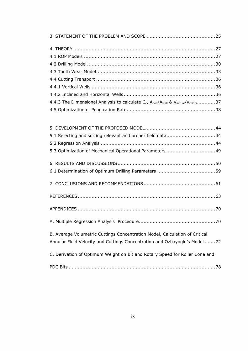
3. STATEMENT OF THE PROBLEM AND SCOPE .............................................25
4. THEORY .............................................................................................27
4.1 ROP Models ......................................................................................27
4.2 Drilling Model ....................................................................................30
4.3 Tooth Wear Model..............................................................................33
4.4 Cutting Transport ..............................................................................36
4.4.1 Vertical Wells .................................................................................36
4.4.2 Inclined and Horizontal Wells ............................................................36
4.4.3 The Dimensional Analysis to calculate Cc, Abed/Awell & Vactual/Vcritical...........37
4.5 Optimization of Penetration Rate..........................................................38
5. DEVELOPMENT OF THE PROPOSED MODEL..............................................44
5.1 Selecting and sorting relevant and proper field data................................44
5.2 Regression Analysis ...........................................................................44
5.3 Optimization of Mechanical Operational Parameters ................................49
6. RESULTS AND DISCUSSIONS................................................................50
6.1 Determination of Optimum Drilling Parameters ......................................59
7. CONCLUSIONS AND RECOMMENDATIONS...............................................61
REFERENCES..........................................................................................63
APPENDICES ..........................................................................................70
A. Multiple Regression Analysis Procedure..................................................70
B. Average Volumetric Cuttings Concentration Model, Calculation of Critical
Annular Fluid Velocity and Cuttings Concentration and Ozbayoglu’s Model .......72
C. Derivation of Optimum Weight on Bit and Rotary Speed for Roller Cone and
PDC Bits ................................................................................................78
x
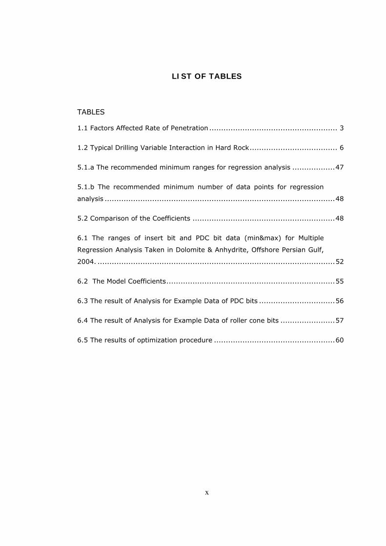
LIST OF TABLES
TABLES
1.1 Factors Affected Rate of Penetration ...................................................... 3
1.2 Typical Drilling Variable Interaction in Hard Rock..................................... 6
5.1.a The recommended minimum ranges for regression analysis ..................47
5.1.b The recommended minimum number of data points for regression
analysis .................................................................................................48
5.2 Comparison of the Coefficients ............................................................48
6.1 The ranges of insert bit and PDC bit data (min&max) for Multiple
Regression Analysis Taken in Dolomite & Anhydrite, Offshore Persian Gulf,
2004. ....................................................................................................52
6.2 The Model Coefficients.......................................................................55
6.3 The result of Analysis for Example Data of PDC bits ................................56
6.4 The result of Analysis for Example Data of roller cone bits .......................57
6.5 The results of optimization procedure ...................................................60
xi
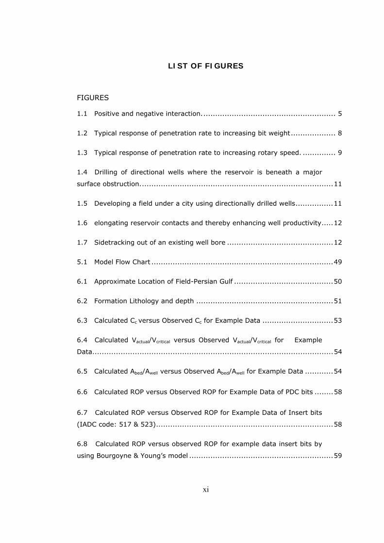
LIST OF FIGURES
FIGURES
1.1 Positive and negative interaction......................................................... 5
1.2 Typical response of penetration rate to increasing bit weight................... 8
1.3 Typical response of penetration rate to increasing rotary speed. .............. 9
1.4 Drilling of directional wells where the reservoir is beneath a major
surface obstruction..................................................................................11
1.5 Developing a field under a city using directionally drilled wells................11
1.6 elongating reservoir contacts and thereby enhancing well productivity.....12
1.7 Sidetracking out of an existing well bore .............................................12
5.1 Model Flow Chart .............................................................................49
6.1 Approximate Location of Field-Persian Gulf ..........................................50
6.2 Formation Lithology and depth ..........................................................51
6.3 Calculated Cc versus Observed Cc for Example Data ..............................53
6.4 Calculated Vactual/Vcritical versus Observed Vactual/Vcritical for Example
Data......................................................................................................54
6.5 Calculated Abed/Awell versus Observed Abed/Awell for Example Data ............54
6.6 Calculated ROP versus Observed ROP for Example Data of PDC bits ........58
6.7 Calculated ROP versus Observed ROP for Example Data of Insert bits
(IADC code: 517 & 523)...........................................................................58
6.8 Calculated ROP versus observed ROP for example data insert bits by
using Bourgoyne & Young’s model .............................................................59
xii
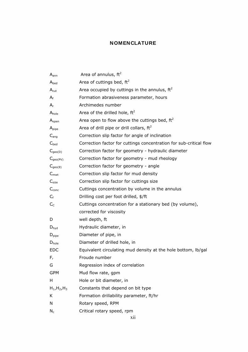
NOMENCLATURE
Aann Area of annulus, ft2
Abed Area of cuttings bed, ft2
Acut Area occupied by cuttings in the annulus, ft2
Af Formation abrasiveness parameter, hours
Ar Archimedes number
Ahole Area of the drilled hole, ft2
Aopen Area open to flow above the cuttings bed, ft2
Apipe Area of drill pipe or drill collars, ft2
Cang Correction slip factor for angle of inclination
Cbed Correction factor for cuttings concentration for sub-critical flow
Cgeo(D) Correction factor for geometry - hydraulic diameter
Cgeo(PV) Correction factor for geometry - mud rheology
Cgeo(θ) Correction factor for geometry - angle
Cmwt Correction slip factor for mud density
Csize Correction slip factor for cuttings size
Cconc Cuttings concentration by volume in the annulus
Cf Drilling cost per foot drilled, $/ft
CC Cuttings concentration for a stationary bed (by volume),
corrected for viscosity
D well depth, ft
Dhyd Hydraulic diameter, in
Dpipe Diameter of pipe, in
Dhole Diameter of drilled hole, in
EDC Equivalent circulating mud density at the hole bottom, lb/gal
Fr Froude number
G Regression index of correlation
GPM Mud flow rate, gpm
H Hole or bit diameter, in
H1,H2,H3 Constants that depend on bit type
K Formation drillability parameter, ft/hr
N Rotary speed, RPM
Nc Critical rotary speed, rpm
xiii
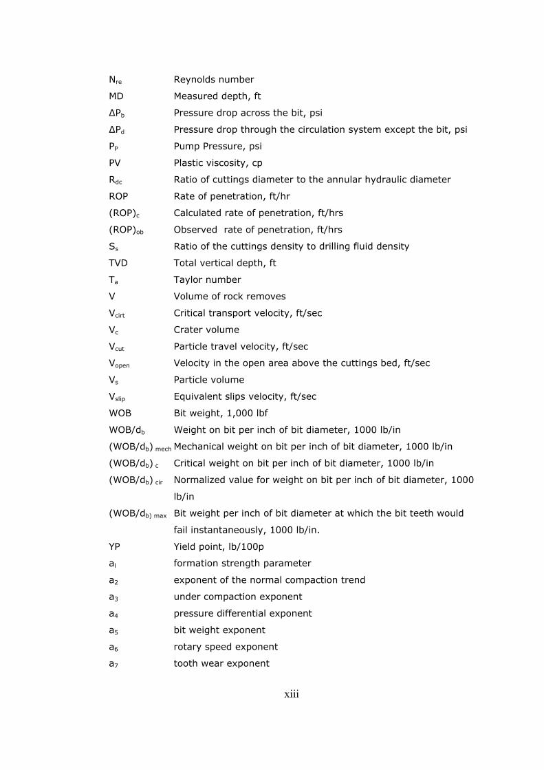
Nre Reynolds number
MD Measured depth, ft
ΔPb Pressure drop across the bit, psi
ΔPd Pressure drop through the circulation system except the bit, psi
PP Pump Pressure, psi
PV Plastic viscosity, cp
Rdc Ratio of cuttings diameter to the annular hydraulic diameter
ROP Rate of penetration, ft/hr
(ROP)c Calculated rate of penetration, ft/hrs
(ROP)ob Observed rate of penetration, ft/hrs
Ss Ratio of the cuttings density to drilling fluid density
TVD Total vertical depth, ft
Ta Taylor number
V Volume of rock removes
Vcirt Critical transport velocity, ft/sec
Vc Crater volume
Vcut Particle travel velocity, ft/sec
Vopen Velocity in the open area above the cuttings bed, ft/sec
Vs Particle volume
Vslip Equivalent slips velocity, ft/sec
WOB Bit weight, 1,000 lbf
WOB/db Weight on bit per inch of bit diameter, 1000 lb/in
(WOB/db) mech Mechanical weight on bit per inch of bit diameter, 1000 lb/in
(WOB/db) c Critical weight on bit per inch of bit diameter, 1000 lb/in
(WOB/db) cir Normalized value for weight on bit per inch of bit diameter, 1000
lb/in
(WOB/db) max Bit weight per inch of bit diameter at which the bit teeth would
fail instantaneously, 1000 lb/in.
YP Yield point, lb/100p
al formation strength parameter
a2 exponent of the normal compaction trend
a3 under compaction exponent
a4 pressure differential exponent
a5 bit weight exponent
a6 rotary speed exponent
a7 tooth wear exponent
xiv
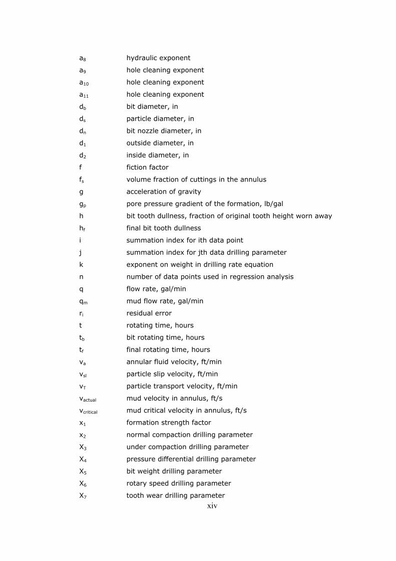
a8 hydraulic exponent
a9 hole cleaning exponent
a10 hole cleaning exponent
a11 hole cleaning exponent
db bit diameter, in
ds particle diameter, in
dn bit nozzle diameter, in
d1 outside diameter, in
d2 inside diameter, in
f fiction factor
fs volume fraction of cuttings in the annulus
g acceleration of gravity
gp pore pressure gradient of the formation, lb/gal
h bit tooth dullness, fraction of original tooth height worn away
hf final bit tooth dullness
i summation index for ith data point
j summation index for jth data drilling parameter
k exponent on weight in drilling rate equation
n number of data points used in regression analysis
q flow rate, gal/min
qm mud flow rate, gal/min
ri residual error
t rotating time, hours
tb bit rotating time, hours
tf final rotating time, hours
va annular fluid velocity, ft/min
vsl particle slip velocity, ft/min
vT particle transport velocity, ft/min
vactual mud velocity in annulus, ft/s
vcritical mud critical velocity in annulus, ft/s
x1 formation strength factor
x2 normal compaction drilling parameter
X3 under compaction drilling parameter
X4 pressure differential drilling parameter
X5 bit weight drilling parameter
X6 rotary speed drilling parameter
X7 tooth wear drilling parameter
xv
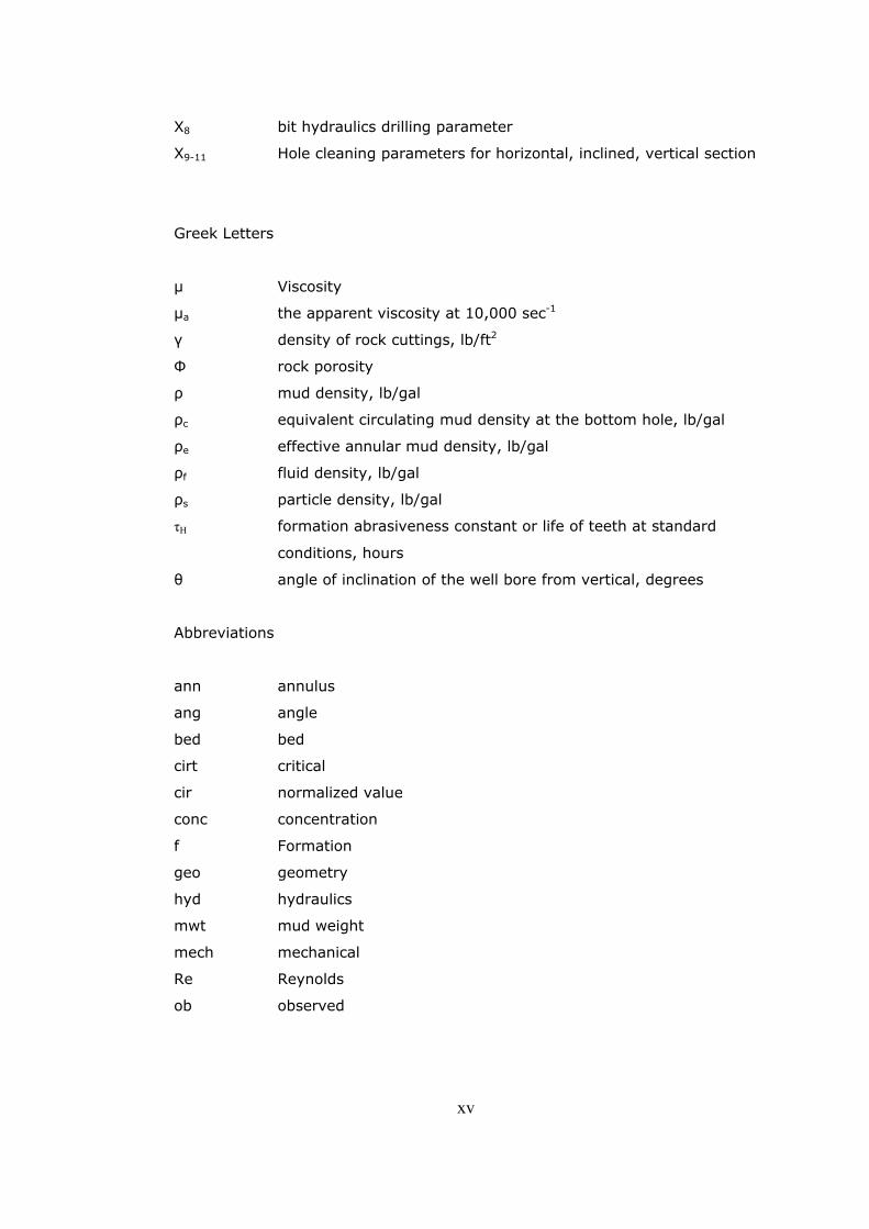
X8 bit hydraulics drilling parameter
X9-11 Hole cleaning parameters for horizontal, inclined, vertical section
Greek Letters
µ Viscosity
µa the apparent viscosity at 10,000 sec-1
γ density of rock cuttings, lb/ft2
Φ rock porosity
ρ mud density, lb/gal
ρc equivalent circulating mud density at the bottom hole, lb/gal
ρe effective annular mud density, lb/gal
ρf fluid density, lb/gal
ρs particle density, lb/gal
τH formation abrasiveness constant or life of teeth at standard
conditions, hours
θ angle of inclination of the well bore from vertical, degrees
Abbreviations
ann annulus
ang angle
bed bed
cirt critical
cir normalized value
conc concentration
f Formation
geo geometry
hyd hydraulics
mwt mud weight
mech mechanical
Re Reynolds
ob observed
CHAPTER I
INTRODUCTION
1.1 What is a drilling operation?
By the name of a well (borehole) is meant a cylindrical mine opening
made too small for man’s access thereto, the diameter of the opening being
many times less than its length. Drilling process is conducted by using
machinery, called drill rig, which consists of a combination of numerous
systems working together. It is the drill collars, screwed onto the bottom of
the drill pipe assembly just above the bit, that provide the necessary weight,
and prevent buckling of the drill pipes above them. Drill collars, along with drill
pipe and bit all make up the drill string, which is rotated by the rotary table
and the Kelly. The drill string component parts are hollow down the middle so
that the drilling fluid can be circulated down to the bit. A fluid-tight rotary
joint, the swivel, is located at the top of the Kelly and provides a connection
between the mud pump discharge line and the inside of the drill string. A
hoisting system is required to support the weight of the drill string, lower it
into the hole and pull it out. This is the function of the derrick, the hook and
the draw works.
The drilling rig is complete with facilities to treat the drilling fluid when it
gets back to the surface, a storage area for tubular goods, shelters and offices
on site.
In addition, when a well is being drilled, it is regularly cased. It is lined
with steel pipe, or casing, which is lowered into the hole under its own weight
in smaller and smaller diameters as the hole gets deeper. The first length of
pipe is run in as soon as the bit has drilled the surface formation and is then
cemented in the hole. A casing housing is connected to the top of the surface
2
casing. All the following lengths of pipe are hung on the casing housing and
cemented at the base to the walls of the hole.
After the first drilling phase is cased, drilling will be resumed with a bit
with a diameter smaller than the inside diameter of the casing string that was
run in and cemented. The deeper the borehole gets and the more casings are
set in the well, the smaller the diameter of the bit must be.
In order to drill a well, three factors have to be established
simultaneously; i) a certain load has to be applied on the bit, ii) the bit has to
be rotated, and iii) a drilling fluid has to be circulated within the well bore.
Making a hole for the recovery of underground oil and gas is a process
which requires two major constituents; i) man-power, and ii) hardware
systems. The man power includes a drilling engineering group and a rig
operator group. The first provides engineering support for optimum drilling
operations, including rig selection, design of mud program, casing and cement
programs, hydraulic program, drill bit program, drill string program and well
control program. After drilling begins, the daily operations are handled by a rig
operator group which consists of a tool pusher and several drilling crews. The
hardware systems which make up a rotary drilling rig are i) power generation
system, ii) hoisting system, iii) drilling fluid circulation system, iv) rotary
system, v) well blowout control system, and vi) drilling data acquisition system
and monitoring system.
As regards their purpose, boreholes drilled for geological exploration of
the region, search for, prospecting and exploitation of deposits are classified
into key or stratigraphic, extension or outpost, structure-exploratory,
reconnaissance, prospecting production and special boreholes.
1.2 Factors Affecting Penetration Rate
The factors which are influencing ROP can be classified in two main
groups: i) Controllable Factors, and ii) Environmental Factors. Table 1.1 lists
these factors. The controllable factors can be altered more easily than
environmental factors. Because of economical and geological conditions, the
variation of environmental factors is impractical or expensive. The number of
3
factors hints at the complexity of the bit/rock interaction, something which is
compounded by interdependence and nonlinearity in some of these effects
[11]. Since mud properties, such as type, density, etc, are all dependent on
formation type, formation pressure, etc, mud properties are included in
“Environmental Factors” in Table 1.1.
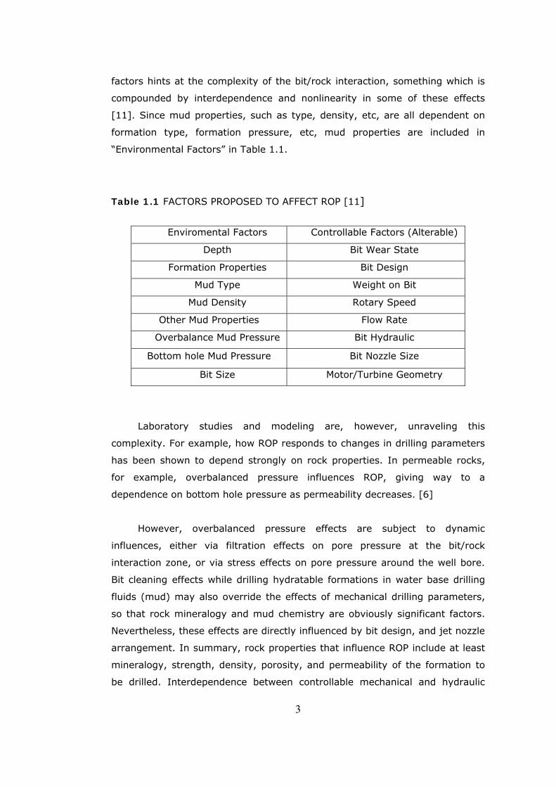
Table 1.1 FACTORS PROPOSED TO AFFECT ROP [11]
Enviromental Factors Controllable Factors (Alterable)
Depth Bit Wear State
Formation Properties Bit Design
Mud Type Weight on Bit
Mud Density Rotary Speed
Other Mud Properties Flow Rate
Overbalance Mud Pressure Bit Hydraulic
Bottom hole Mud Pressure Bit Nozzle Size
Bit Size Motor/Turbine Geometry
Laboratory studies and modeling are, however, unraveling this
complexity. For example, how ROP responds to changes in drilling parameters
has been shown to depend strongly on rock properties. In permeable rocks,
for example, overbalanced pressure influences ROP, giving way to a
dependence on bottom hole pressure as permeability decreases. [6]
However, overbalanced pressure effects are subject to dynamic
influences, either via filtration effects on pore pressure at the bit/rock
interaction zone, or via stress effects on pore pressure around the well bore.
Bit cleaning effects while drilling hydratable formations in water base drilling
fluids (mud) may also override the effects of mechanical drilling parameters,
so that rock mineralogy and mud chemistry are obviously significant factors.
Nevertheless, these effects are directly influenced by bit design, and jet nozzle
arrangement. In summary, rock properties that influence ROP include at least
mineralogy, strength, density, porosity, and permeability of the formation to
be drilled. Interdependence between controllable mechanical and hydraulic

4
drilling parameter effects may also be significant, such as the response of ROP
to weight on bit (WOB), rotary speed and flow rate is directly depend on
absolute value of these parameters. Bit design effects are also not well
understood. Differences in bit design effects on ROP with polycrystalline
diamond compact (PDC) bits appear only to become significant when bit
surface cleaning problems occur, or when cutters become worn, while with
roller cone bits, also jet nozzle arrangement should be considered. [24]
Finally, complexity is increased by errors and inconsistencies in drilling
data, meaning that correlations with ROP may be masked without extensive
data treatment. Accuracy of the equipment used for data acquisition as well as
heterogeneities and insufficient information about the formations cause such
problems. This latter point may explain why, despite number of analytically
derived ROP models published, none has yet become established as a
comprehensive operational tool. [24]
The complexity of the bit/rock interaction, and the difficulties with
implementation of analytical models, have encouraged professional people to
adopt an empirical approach to optimize ROP in drilling operations. This
methodology is usually conducted as follows: i) grouping of data according to
the formations, i.e., analysis should be conducted for each drilled formation
separately, ii) development of dimensionless groups, and iii) determination of
the model constants using the collected data by the help of statistical tools.
[24]
Emphasis has also been placed in this work on understanding the effects
of controllable variables, i.e., those that can be readily changed to optimize
ROP. Other environmental effects are however incorporated into another ROP
modeling technique developed by Professional people and described
elsewhere. [24]
In considering which variables to choose for developing an ROP model,
experience and research suggest these eight variables: i) Mud Properties, ii)
Hydraulics, iii) Bit type, iv) Weight on Bit, v) Drill string Rotation Speed, vi)
Depth, vii) Bit tooth wear, and vii) Formation Properties. However, for
horizontal and inclined well bores, hole cleaning is also a major factor
influencing the ROP. The basic interactive effects between these variables
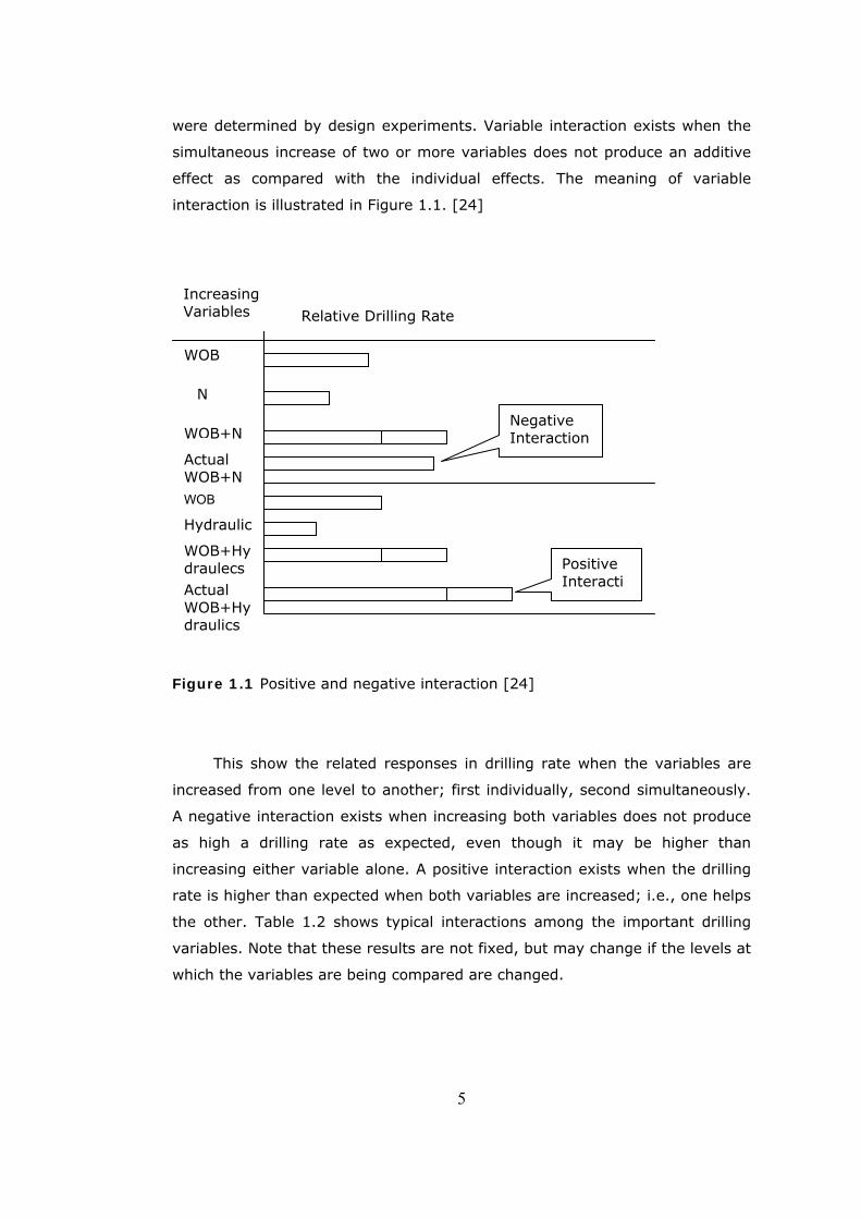
were determined by design experiments. Variable interaction exists when the
simultaneous increase of two or more variables does not produce an additive
effect as compared with the individual effects. The meaning of variable
interaction is illustrated in Figure 1.1. [24]
WOB
N
Actual WOB+N
Negative Interaction
WOB
Hydraulics WOB+Hydraulecs Positive
Interacti
Relative Drilling Rate
Actual WOB+Hydraulics
WOB+N
Increasing Variables
Figure 1.1 Positive and negative interaction [24]
This show the related responses in drilling rate when the variables are
increased from one level to another; first individually, second simultaneously.
A negative interaction exists when increasing both variables does not produce
as high a drilling rate as expected, even though it may be higher than
increasing either variable alone. A positive interaction exists when the drilling
rate is higher than expected when both variables are increased; i.e., one helps
the other. Table 1.2 shows typical interactions among the important drilling
variables. Note that these results are not fixed, but may change if the levels at
which the variables are being compared are changed.
5
6
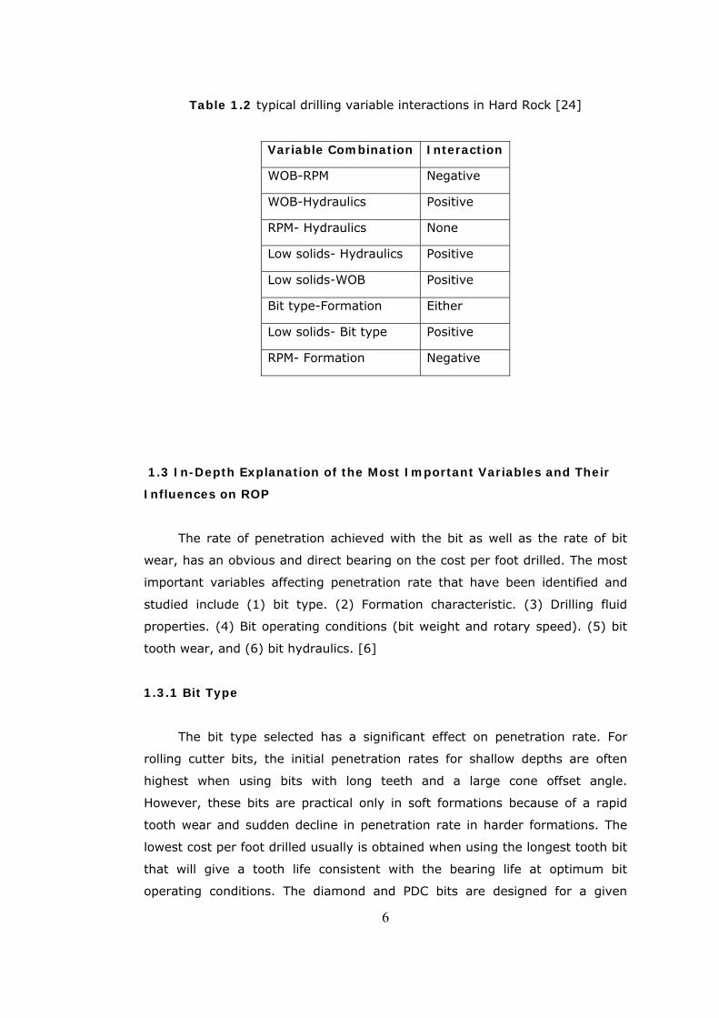
Table 1.2 typical drilling variable interactions in Hard Rock [24]
Variable Combination Interaction
WOB-RPM Negative
WOB-Hydraulics Positive
RPM- Hydraulics None
Low solids- Hydraulics Positive
Low solids-WOB Positive
Bit type-Formation Either
Low solids- Bit type Positive
RPM- Formation Negative
1.3 In-Depth Explanation of the Most Important Variables and Their
Influences on ROP
The rate of penetration achieved with the bit as well as the rate of bit
wear, has an obvious and direct bearing on the cost per foot drilled. The most
important variables affecting penetration rate that have been identified and
studied include (1) bit type. (2) Formation characteristic. (3) Drilling fluid
properties. (4) Bit operating conditions (bit weight and rotary speed). (5) bit
tooth wear, and (6) bit hydraulics. [6]
1.3.1 Bit Type
The bit type selected has a significant effect on penetration rate. For
rolling cutter bits, the initial penetration rates for shallow depths are often
highest when using bits with long teeth and a large cone offset angle.
However, these bits are practical only in soft formations because of a rapid
tooth wear and sudden decline in penetration rate in harder formations. The
lowest cost per foot drilled usually is obtained when using the longest tooth bit
that will give a tooth life consistent with the bearing life at optimum bit
operating conditions. The diamond and PDC bits are designed for a given
7
penetration per revolution by the selection of the size and number of
diamonds or PDC blanks. The width and number of cutters can be used to
compute the effective number of blades. The length of the cutters projecting
from the face of the bit (less the bottom clearance) limited the depth of the
cut. The PDC bits perform best in soft, firm, and medium-hard, nonabrasive
formations that are not “gummy”. [6]
1.3.2 Formation Characteristics
The elastic limit and ultimate strength of the formation are the most
important formation properties affecting penetration rate. It is mentioned that
the crater volume produced beneath a single tooth is inversely proportional to
both the compressive strength of the rock and the shear strength of the rock.
The permeability of the formation also has a significant effect on the
penetration rate. In permeable rocks, the drilling fluid filtrate can move into
the rock ahead of the bit and equalize the pressure differential acting on the
chips formed beneath each tooth. It also can be argued that the nature of the
fluid contained in the pore space of the rock also affects this mechanism since
more filtrate volume would be required to equalize the pressure in a rock
containing gas than in a rock containing liquid. The mineral composition of the
rock also has some effect on penetration rate. [6]
1.3.3 Drilling Fluid Properties
The properties of the drilling fluid reported to affect the penetration rate
include (l) density, (2) rheological flow properties, (3) filtration characteristics,
(4) solids content and size distribution, and (5) chemical composition.
Penetration rate tends to decrease with increasing fluid density, viscosity, and
solids content, and tends to increase with increasing filtration rate. The
density, solids content, and filtration characteristics of the mud control the
pressure differential across the zone of crushed rock beneath the bit. The fluid
viscosity controls the parasitic frictional losses in the drill string and, thus, the
hydraulic energy available at the bit jets for cleaning. There is also
experimental evidence that increasing viscosity reduces penetration rate even
when the bit is perfectly clean. The chemical composition of the fluid has an
effect on penetration rate, such that the hydration rate and bit ballling
tendency of some clays are affected by the chemical composition of the fluid.
An increase in drilling fluid density causes a decrease in penetration rate for
rolling cutter bit. An increase in drilling fluid density causes an increase in the
bottom hole pressure beneath the bit and, thus, an increase in the pressure
differential between the borehole pressure and the formation fluid pressure.
[6]
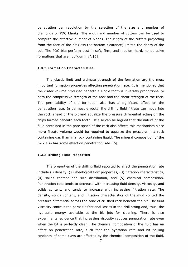
1.3.4 Operating Conditions (WOB & Rotary Speed)
A typical plot of penetration rate versus bit weight obtained
experimentally with all other drilling variables held constant is shown in Fig.
1.2. No significant penetration rate is obtained until the threshold bit weight is
applied (Point a). Penetration rate, then, increases with increasing values of
bit weight (Segment a-b). As the weight on bit values are increased, a higher
increase in ROP is observed (Segment b-c). However, after a certain value of
bit weight, subsequent increase in bit weight causes only slight improvements
in penetration rate (Segment c-d). In some cases, a decrease in penetration
rate is observed at extremely high values of bit weight (Segment d-e). This
type of behavior often is called bit floundering. The poor response of
penetration rate at high values of bit weight usually is attributed to less
efficient bottom hole cleaning at higher rates of cuttings generation or to a
complete penetration of the cutting elements of the bit into the well bore
bottom. At this weight on bit values, wear on the bit is extremely high. [6]
RO
P
d
a
WOB
c
b
c
Figure 1.2 Typical response of penetration rate to increasing bit weight [6]
8
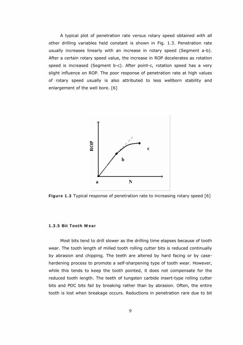
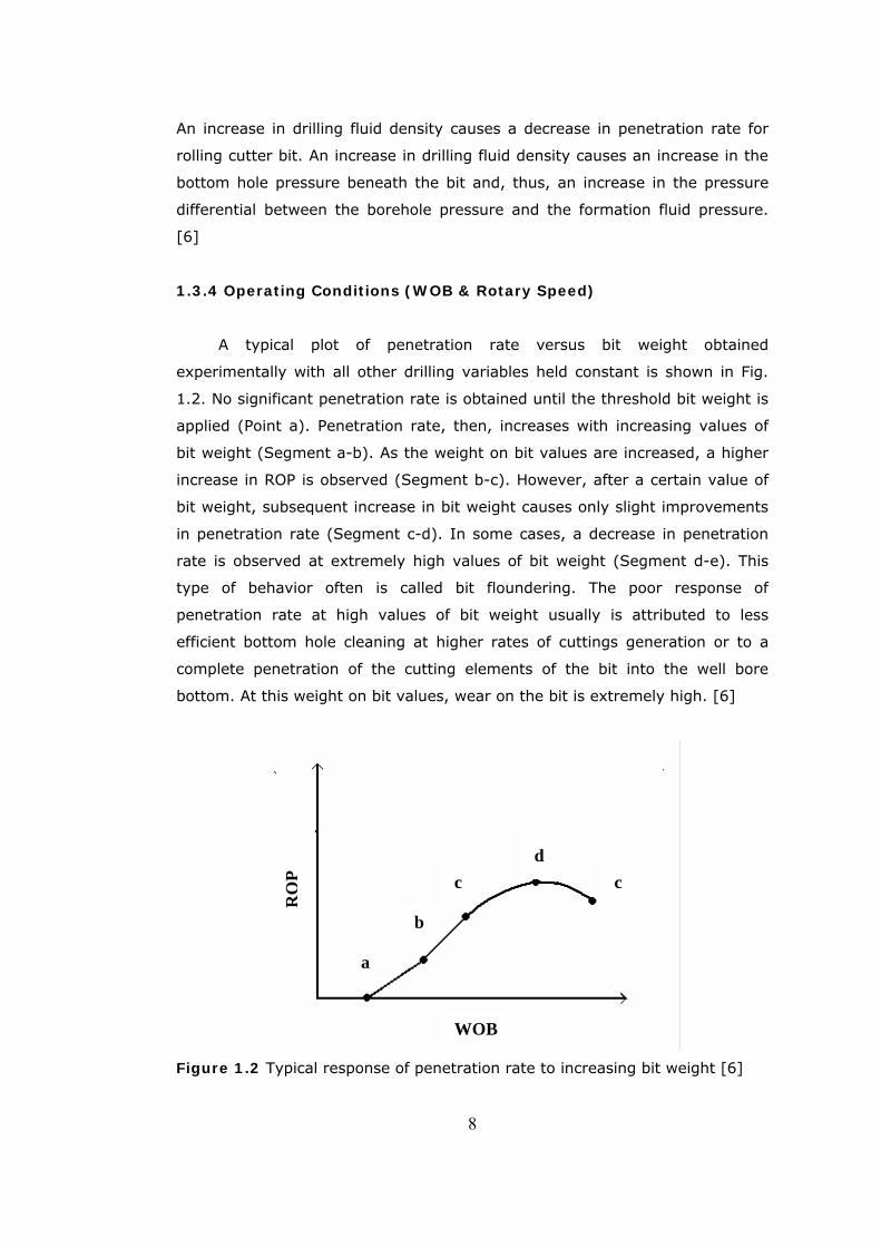
A typical plot of penetration rate versus rotary speed obtained with all
other drilling variables held constant is shown in Fig. 1.3. Penetration rate
usually increases linearly with an increase in rotary speed (Segment a-b).
After a certain rotary speed value, the increase in ROP decelerates as rotation
speed is increased (Segment b-c). After point-c, rotation speed has a very
slight influence on ROP. The poor response of penetration rate at high values
of rotary speed usually is also attributed to less wellborn stability and
enlargement of the well bore. [6]
RO
P
c
N
b
a
Figure 1.3 Typical response of penetration rate to increasing rotary speed [6]
1.3.5 Bit Tooth Wear
Most bits tend to drill slower as the drilling time elapses because of tooth
wear. The tooth length of milled tooth rolling cutter bits is reduced continually
by abrasion and chipping. The teeth are altered by hard facing or by case-
hardening process to promote a self-sharpening type of tooth wear. However,
while this tends to keep the tooth pointed, it does not compensate for the
reduced tooth length. The teeth of tungsten carbide insert-type rolling cutter
bits and PDC bits fail by breaking rather than by abrasion. Often, the entire
tooth is lost when breakage occurs. Reductions in penetration rare due to bit
9
10
wear usually are not as severe for insert bits as for milled tooth bits unless a
large number of teeth are broken during the bit run. [6]
1.3.6 Bit Hydraulics
Significant improvements in penetration rate could be achieved by a
proper jetting action at the bit. The improved jetting action promoted better
cleaning of the bit face as well as the hole bottom. There exists an uncertainty
on selection of the best proper hydraulic objective function to be used in
characterizing the effect of hydraulics on penetration rate. Bit hydraulic
horsepower, jet impact force, Reynolds number, etc, are commonly used
objective functions for describing the influence of bit hydraulics on ROP. [6]
1.4 Directional and Horizontal Well Drilling
Recently, with the advancement of industrial techniques, the number of
inclined and horizontal wells has been increased. Common application fields for
directional and horizontal drilling are in offshore and onshore when there is no
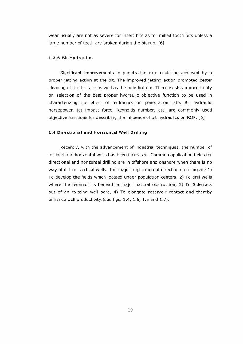
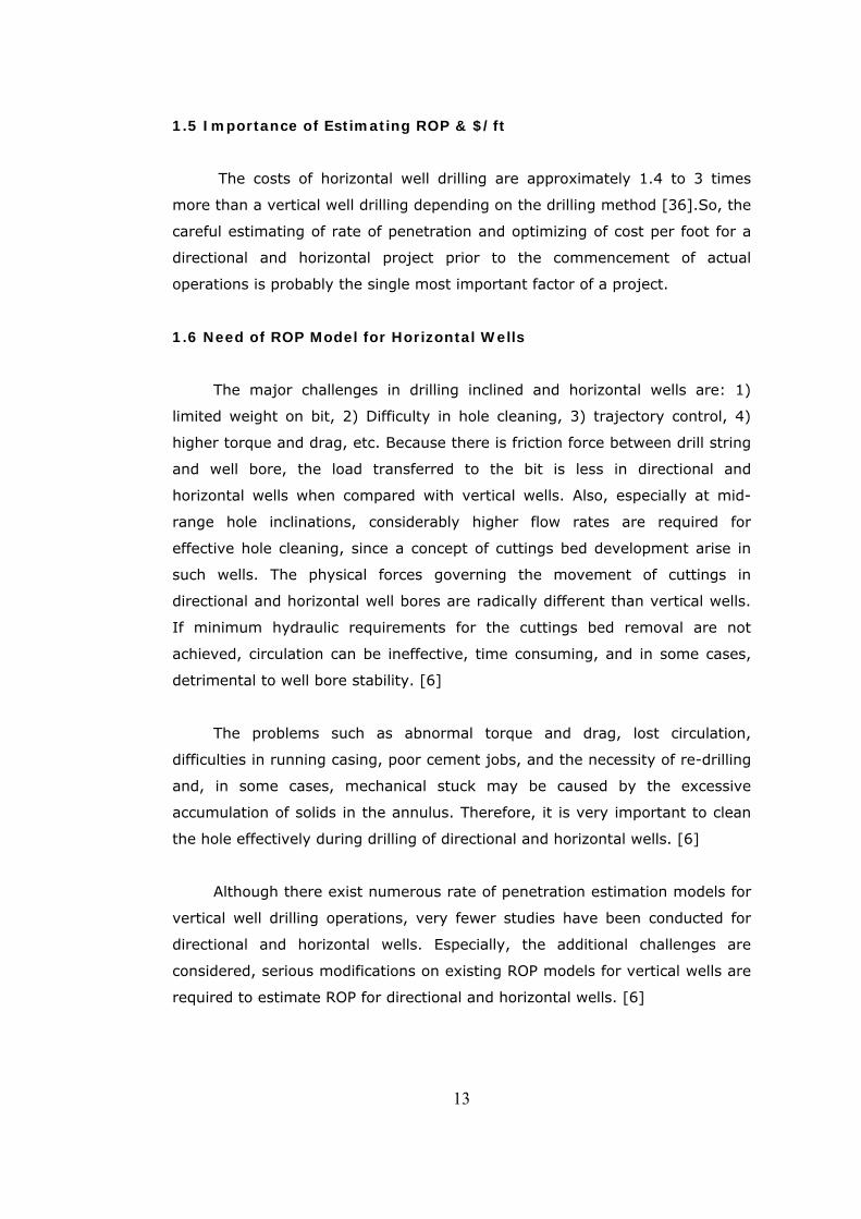
way of drilling vertical wells. The major application of directional drilling are 1)
To develop the fields which located under population centers, 2) To drill wells
where the reservoir is beneath a major natural obstruction, 3) To Sidetrack
out of an existing well bore, 4) To elongate reservoir contact and thereby
enhance well productivity.(see figs. 1.4, 1.5, 1.6 and 1.7).
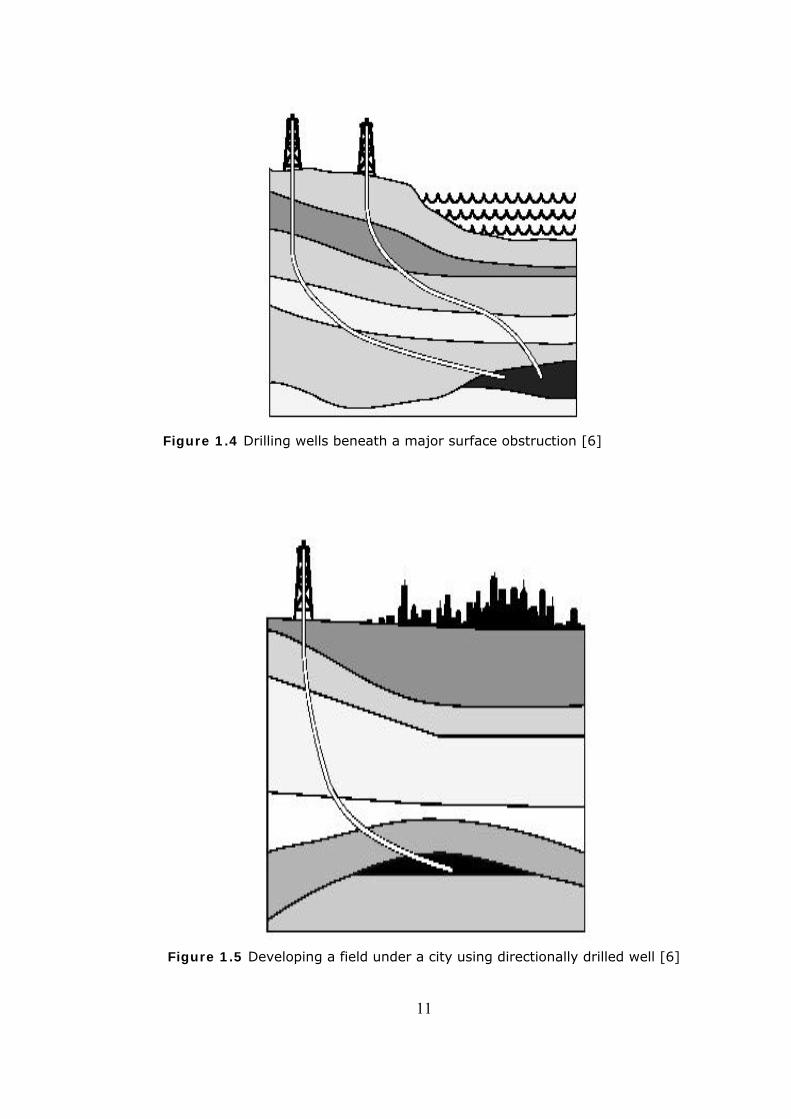
Figure 1.4 Drilling wells beneath a major surface obstruction [6]
Figure 1.5 Developing a field under a city using directionally drilled well [6]
11
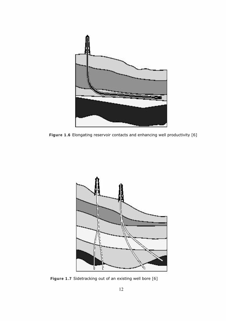
Figure 1.6 Elongating reservoir contacts and enhancing well productivity [6]
Figure 1.7 Sidetracking out of an existing well bore [6]
12
13
1.5 Importance of Estimating ROP & $/ft
The costs of horizontal well drilling are approximately 1.4 to 3 times
more than a vertical well drilling depending on the drilling method [36].So, the
careful estimating of rate of penetration and optimizing of cost per foot for a
directional and horizontal project prior to the commencement of actual
operations is probably the single most important factor of a project.
1.6 Need of ROP Model for Horizontal Wells
The major challenges in drilling inclined and horizontal wells are: 1)
limited weight on bit, 2) Difficulty in hole cleaning, 3) trajectory control, 4)
higher torque and drag, etc. Because there is friction force between drill string
and well bore, the load transferred to the bit is less in directional and
horizontal wells when compared with vertical wells. Also, especially at mid-
range hole inclinations, considerably higher flow rates are required for
effective hole cleaning, since a concept of cuttings bed development arise in
such wells. The physical forces governing the movement of cuttings in
directional and horizontal well bores are radically different than vertical wells.
If minimum hydraulic requirements for the cuttings bed removal are not
achieved, circulation can be ineffective, time consuming, and in some cases,
detrimental to well bore stability. [6]
The problems such as abnormal torque and drag, lost circulation,
difficulties in running casing, poor cement jobs, and the necessity of re-drilling
and, in some cases, mechanical stuck may be caused by the excessive
accumulation of solids in the annulus. Therefore, it is very important to clean
the hole effectively during drilling of directional and horizontal wells. [6]
Although there exist numerous rate of penetration estimation models for
vertical well drilling operations, very fewer studies have been conducted for
directional and horizontal wells. Especially, the additional challenges are
considered, serious modifications on existing ROP models for vertical wells are
required to estimate ROP for directional and horizontal wells. [6]
14
CHAPTER II
LITERATURE REVIEW
An extensive literature review was carried out in order to determine the
state of the art on the subject. Because of the vast number of articles in these
areas, this literature review is limited to the most relevant and/or well known
works.
2.1 Mechanical Parameters
Galle and Woods [13] presented a pioneer work that created a major
breakthrough in drilling technology, mainly when referring to optimization
aspects. They assumed that rate of penetration was affected by only two
parameters, weight on bit and rotary speed. In their paper, also, it is assumed
that all other variables involved, like bit selection, hydraulics, drilling fluid
properties, etc., were properly selected. They defined an analytical model to
predict rate of penetration (ROP) as a function of weight on bit, rotary speed,
type of formation, and bit tooth wear.
Maurer [29] derived an equation for rate of penetration for roller-cone
bits from rock cratering mechanisms. This equation holds for “perfect
cleaning”, which is defined as the condition where all of the rock debris is
removed from the bottom hole.
Galle and Woods [14] followed the similar procedures that they used in
their early 1960 paper. They presented procedures for determining the best
combination of constant weight on bit and rotary speed, the best constant
weight on bit for any given rotary speed, and the best constant rotary speed
for any given bit weight analytically. For each of these procedures, they
presented eight cases considering a combination of bit teeth and bearing life,
such that drilling rate limits economical bit life. They established empirical
equations for the effects of weight on bit, rotary speed, and cutter structure
dullness on drilling rate, rate of tooth wear and bearing life.
Mechem and Fullerton [30] introduced a rate of penetration model
based on formation drill ability, bit weight, rotary speed, well depth, mud
pressure, and applied hydraulics. Their model is using a concept based on a
single expression of drilling energy-level, the NWOB × product that can be
related to those variables using graphical methods. These correlations provide
the basis of for determining hydraulic requirements, estimating drilling cost,
basic well planning, and drilling optimization.
Langston [23] described a methodology for managing daily drilling data
as well as existing information collected from the very same field. He indicated
that during analysis of actual drilling data, none of the drilling variables could
be excluded due to the simultaneous interaction of each and every variable
among themselves. In practice, procedures interrelate and depend upon each
other as well as on personnel and mechanical factors.
Young [55] described a computer control system for collecting and
analyzing the field data, and presented a real case application. He developed a
solution for minimum-cost drilling assuming constant bit weight and rotary
speed over the entire bit life for roller cone and PDC bits. The proposed
solution is depended on four equations, i.e., drilling rate, bit bearing wear, bit
tooth wear, and cost.
15
Lummus [24] presented the definition and philosophy of optimization. He
discussed the influence of major drilling parameters on drilling performance.
He also proposed a drilling optimization methodology. In this paper, data
required for drilling optimization were obtained from i) Logs (preferably IES or
sonic), ii) Bit records, iii) Mud records, iv) Recorded drilling data, such as
torque, pump pressure, penetration rate, etc., v) Drilling program for
proposed well, i.e., casing setting depths, hole size, expected problems, etc.,
vi) Rig specifications, and vii) Correlation of formation characteristics of the
well.
Lummus [25] discussed the acquisition and analysis of data needed to
plan, maintain, and appraise the drilling of a particular well. The data required
for optimized drilling are classified as follows: i) Data needed for computer
input to calculate optimum values for the controllable drilling conditions, ii)
Data needed on a day-by-day basis to determine how efficiently drilling
optimization is being applied and to provide the basis for suggested changes in
mud, hydraulics, bits, etc., and iii) Data needed to evaluate the effectiveness
of an optimum drilling program for a particular well and to develop definite
recommendations for improving drilling efficiency on future wells.
Wilson and Bentsen [51] presented optimization techniques for
minimizing drilling costs by restricting the number of parameters to be
optimized to two, namely, the weight on the bit and the rotary speed. In this
study, three methods of varying complexity have been developed. The first
method seeks to minimize the cost per foot drilled during a bit run. The second
method minimizes the cost of a selected interval, and the third method
minimizes the cost over a series of intervals. The methods are listed in order
to increase complexity. It was found that each of the methods gave a
worthwhile cost saving and that the saving increased as the complexity of the
method increased. The data requirements for the method increased with
increasing method complexity.
In order to have the least cost per foot, Reed [40] developed a method
to find the best combination of weight on bit and rotary speed in two cases,
constant or variable parameters. His method agreed very well with results
from Galle and Woods papers, but it was considered to be more precise
because the equations were solved in a more rigorous way using a Monte
Carlo Scheme. This paper also showed that there is little advantage in using
variable weight speed technology over the simpler constant weight-speed
method, if the formation is homogenous.
16
Hal B. Fullerton [12] followed the similar procedures that he used in their
early 1965 paper. He presented relationship between weight on bit, rotary
speed, rate of penetration, and apparent rock drill ability (Kf).In this study, it
is assumed that ,within normal operating ranges, any value may be
considered a constant. Also, effect of hydrostatic pressure on apparent rock
drill ability and effects of bit hydraulic horsepower and tooth wearing on
NWOB ×
NWOB × are represented by related equations and graphs. Bit records
obtained from wells in an area of interest are used to test the accuracy of
model.
Bourgoyne and Young[5] developed a mathematical model, using a
multiple regression analysis technique of detailed drilling data, to describe the
drilling rate based on formation depth, formation strength, formation
compaction, pressure differential across the bottom hole, bit diameter and bit
weight, rotary speed, bit wear and bit hydraulics. As a function of these eight
parameters, a mathematical model was developed in order to find the best
constant weight on bit, rotary speed and optimum hydraulics for a single bit
run in order to achieve minimum cost per foot. The method also predicts the
drilling hours and bit wear. They considered that more emphasis had been
placed on the collection of detailed drilling data to aid in the selection of
improved drilling practices. Thus, the constants that appear in their model
could be determined from a multiple regression analysis of field data (See
Appendix A). The Bourgoyne& Young model has greater acceptance within the
portion of the drilling industry that uses drilling models at all, because it is one
of the most complete models.
E.Tanseu [48] presented a new approach in formulating and solving the
optimal drilling problem. The approach is heuristic as it involves the interaction
of raw data, regression and an optimization technique. From several bit runs,
regression equations were established for predicting penetration rate and bit
life. Three control variables are accounted for: weight on bit, rotary speed and
bit hydraulic horsepower. The equations for penetration rate and bit life are
incorporated into a drilling cost equation and the cost function is minimized
over the control variables. These variables then dictate the optimal drilling of
the next bit run.
Hoover and Middleton [17] tested experimentally five polycrystalline
diamond Compact (PDC) bit designs in the laboratory at 100and 500 rpm in
three different types of rock: Nugget sandstone, Crab Orchard sandstone, and
Sierra White granite. This paper describes the testing procedures, summarizes
bit performance and wears characteristics, and correlates these experimental
results with specific design options such as rock angle, bit profile, and material
17
18
selection. As the bits develop large wear flats in hard rock, it is concluded that
the torque becomes much more sensitive to changes in the weight on the bit.
Hussein Rabia [18] presented a simplified approach to bit selection that
uses the principle of specific energy. Specific energy (Es) may be defined as
the energy required removing a unit volume of rock. Comparison of bit
selection, based on both cost per foot and specific energy, was made. It can
be indicated that Es can be used to select the proper bit type for any section of
hole, and the switch over points for different bit types may be determined
from the plots of Specific energy vs. depth. Specific energy also can be used
as a criterion for ending the use of a current bit. For this application, Specific
energy can be a more meaningful tool than any other available means, such
as the cumulative cost per foot. The potential application of specific energy in
development and exploration wells was discussed.
S.C, Malguarnera [27] formulated system of equations which describe
the quantitative interactions of the most important parameters of the rotary
drilling process. These equations are based on both laboratory and field
observations. The equations were then incorporated into computer programs
to provide bit run simulation, and operating condition of optimization. Drilling
model which described in this paper provide a systematic way to use
mathematical modeling and computer capability.
Ziaja and Miska [31] presented mathematical model of the
polycrystalline diamond bit drilling process and its practical application.
Expressions for bit torque and bit weight are obtained in terms of bit
penetration rate. The model takes into account the reduction in penetration
rate during drilling resulting from bit wear. Some teats in the field conditions
have shown that theoretical results agree reasonably well with available
experimental data. A graphical method for estimating so-called indexes of rock
properties also has been established.
E.L.Simmons [47] illustrated a technique for synergistically coupling
several optimization parameters, namely optimum hydraulics, weight on the
bit and bit rotation, in order to achieve a higher degree of drilling efficiency.
Formation drill ability and bit type selection are brought out and integrated
with a generally accepted drilling rate equation. None of the technology or
19
concepts brought out in this paper is new. What has been attempted however
is an illustration of how several of these well known concepts should be
sequentially coupled in order to achieve a system for true drilling optimization.
Reza and Alcocer [41] developed a drilling model using dimensional
analysis. The parameters included in the three equations of penetration rate,
rate of bit dulling and rate of bearing wear are weight on bit, rotary speed,
flow rate, bit diameter, bit nozzle diameter, bearing diameter, mud kinematics
viscosity, differential pressure, temperature, and heat transfer coefficient.
They developed dimensionless models for roller cone, PDC and diamond bits.
Brett and Millheim [7] presented a method named Drilling Performance
Curve (DPC) that is a simple powerful tool to assess the drilling performance in
any given area where a consecutive series of similar wells have been drilled.
All the information that is needed to perform the analysis is the sequence
numbers of the well and the time to reach a given depth. This paper presents
some typical examples of DPC’S covering a study of over 30 different areas
(onshore and offshore) including over 2000 wells. From the data, a simple
model for the overall drilling performance was derived It will be shown that
the DPC can dictate the strategy for a drilling program and what the
economics of drilling a sequence of wells should be in a given area.
T.M. Warren [50] developed a model for predicting ROP for roller-cone
bits under low-borehole-pressure conditions. This model accounted for both
cuttings generation and cuttings removal. Drilling data obtained under high-
borehole-pressure conditions were analyzed to determine the reasons of the
reduction in ROP as the borehole pressure increases. In some cases, the
reduced ROP is caused by a buildup of rock debris under the bit. When this
occurs, the ROP can be improved by an increased level of hydraulics. In other
cases, the reduction in ROP seems to be caused by a local catering effect that
is much less responsive to increases in hydraulics. Comparison of model
predictions to the observed ROP can help to identify the mechanism that limits
the ROP and provide insight into ways to improve it.
Winters, Warren and Onya [52] developed a model, which relates roller
cone bit penetration rates to the bit design, the operating conditions, and the
rock mechanics. Rock ductility is identified as a major influence on bit
20
performance. Cone offset is recognized as an important design feature for
drilling ductile rock. The model relates the effect of cone offset and rock
ductility to predict the drilling response of each bit under reasonable
combinations of operating conditions. Field data obtained with roller cone bits
can be interpreted to generate a rock strength log. The rock strength log can
be used in conjunction with the bit model to predict and interpret the drilling
response of roller cone bits.
Wojtanowicz and Kuru [54] developed a new mechanistic drilling for both
roller cone bits and PDC bits. The model was fully explicit with physical
meanings given for al1 constants and functions. The response of the drilling
model to weight-on-bit and cutters removal and the stability of constants were
tested using some field and laboratory data. Also, the concept of maximum bit
performance (UBP) curve was introduced in this paper. The curves represented
maximum values of the average drilling rates for various pre-assumed footage
values. In contrast to elaborate drilling models, the MBP curves are a single,
comprehensive correlation representing drilling bit behavior in a formation. For
calculating purposes, the curves were normalized and thus they became
insensitive to drill ability change vs. depth as well as formation abrasiveness.
The curves were plotted and analyzed for both roller cone bits and PDC bits.
Also, the simple method for using the MBP curves for drilling optimization was
presented.
Guo X.Z. [16] described a theoretical analysis of the penetration-cost
objective function, specifically its first- and second-order differentiability,
convexity, and presents the location and method of searching for optimum
drilling parameter. The model used in this paper is basically the modified
Young’s model which was commonly used for unsealed-roller-cone bits. In this
study, it is expended to insert-tooth bits by graphically processing. This paper
discusses the features and practical significance of a combined isocost graph,
such as determining the maximum economic results for each combination of
bit weight and speed and providing a scientifically sound basis for modifying
drilling parameters. A case study of the Zhong Yuan oil field also is given.
Bonet, Cunha and prado [4] analyzed the drilling cost for the operation
of an entire drilling operation, from its initial to final depth, in homogeneous
formations. The main objective of this work was to find the optimum drilling
21
parameters for each bit used during the drilling operation, the number of bits
to be used and the depth where each bit will be changed. A computer program
was developed to simplify the use of the method.
Wojtanowicz and Kuru [53] presented a new methodology in drilling
optimization using a dynamic programming (the dynamic drilling strategy).
This strategy employs a two-stage optimization procedure, locally for each drill
bit, and totally for the whole well. The program includes the distribution of bit
footage along the well paths, depths of tripping operations, bit-control
algorithms for all bits, and the optimum number of bits per well.
Barragan, Santos and Maidla, E.E. [2] indicated that optimization of
multiple bit runs is more economical than optimization of single bit runs. They
developed a method based on a heuristic approach to seek the optimum
conditions using Monte Carlo Simulation. This method does not depend on a
particular drilling model and has been tested with several models.
Parker, Collins, Pelli and Brancato [38] developed software to assist in
the choice of roller bits and to estimate the optimum weight on bit and
rotational speed. The analysis was based on prior drilling experience in a field,
utilizing the Bourgoyne and Young method. The optimal weight on bit and
rotational speed calculated based on the minimum cost per meter.
2.2 Cuttings Transport
Efficient removal of cuttings from the well bore is one of the major
considerations during both design and operational stages of a drilling process.
Inadequate hole cleaning may give rise to serious drilling problems, like
increase in torque and drag, stuck pipe, loose control on density, difficulty
when running and cementing casing, etc. [8,37]. If the situation is not handled
properly, these problems can ultimately lead to the loss of a well. A single
stuck pipe indecent may cost over million dollars [1]. To avoid such problems,
generated cuttings have to be removed from the well bore by the help of the
drilling fluid. The ability of the fluid to lift such cuttings is generally referred to
as carrying capacity of the drilling fluid. The major factors affecting the
22
carrying capacity of drilling fluids may be listed as fluid annular velocity, hole
inclination, drilling fluid properties, penetration rate, pipe/hole eccentricity,
hole geometry, cuttings properties, and drill pipe rotation speed[49]. In fact,
fluid flow velocity is the dominant drilling variable on hole cleaning due to its
direct relation with the shear stress acting on the cuttings bed [21]. It has
been stated that in order to remove cuttings from a horizontal or a deviated
well bore, a sufficient shear stress should be applied on the cuttings bed
surface in order to lift the particles and erode the developed bed. Such a lifting
process, of course is directly dependent on not only the fluid properties, but
also the cuttings properties, like shape, compaction properties, etc[21,43,44].
Additionally, it is reported that due to the interaction between the drilling
fluids and cuttings, gel formation within the developed cuttings bed occurs,
which significantly increases the required shear force needed to erode the bed,
and lift the cuttings particles up from the bed [43,44]. Studies on cuttings
transport have been in progress during the past 50 years.[37] These studies
can separated into two basic approaches: i) empirical and ii) theoretical.
Tomren, Iyoho and Azar [49] investigated effects of pipe rotation and hole
inclination angle, eccentricity, flow regimes on cuttings transport performance.
Becker, Azar and Okrajni8 conducted experimental study comparing the effects
of fluid rheological parameters (fluid yield point (YP), plastic viscosity (PV),
YP/PV ratio, power law exponent, consistency index, etc.) on annular hole
cleaning using a large scale flow loop. They pointed out that turbulent flow
improved cuttings transport for highly-inclined wellbores, and the effects of
fluid rheology dominated at low inclinations. Sifferman and Becker[9] stated
that the variables influencing cuttings bed thickness were mud annular
velocity, mud density, inclination angle, and drillpipe rotation (with the first
two being the most important). Sanchez [45] examined the effect of drillpipe
rotation on hole cleaning during directional well drilling. He observed that bed
erosion was improved with pipe rotation. He noted that pipe rotation also
caused irregularities in bed thickness along the test section. Yu et al [56]
proposed a new approach to improve the cuttings transport capacity of drilling
fluid in horizontal and inclined wells by attaching gas bubbles to the surface of
drilled cuttings using chemical surfactants.
Also, numerous theoretical and mechanistic models were introduced for
describing the mechanism of bed development and cuttings transport in
inclined and horizontal wells. Two and three layer models are introduced
23
[37,15,19]. Some of these model performances were tested using
experimental data collected in different cuttings flow loops. Also, there were
attempts for determining the critical fluid velocity for preventing bed
development, either theoretically or experimentally. Larsen, Pilehvari and Azar
[22] presented a new cuttings-transport model which predicted critical velocity
needed to keep all cuttings moving for horizontal and high-angle wells. Cho, et
al [9] developed a three-layer model similar to Nguyen and Rahman’s [35]
model. They developed a simulator and compared the results with existing
models as well as the experimental data conducted by other researchers. They
developed charts to determine the lowest possible pressure gradient to serve
as an operational guide for drilling operations. They also observed the
minimum critical velocity for preventing a stationary bed development using
the simulator results. Masuda et al [28] conducted both experimental
investigation and numerical simulation for different flow conditions to
determine the critical fluid velocity in inclined annulus.
Ozbayoglu [36] presented an analysis of bed height in horizontal and
highly-inclined wellbore by using artificial neural network. In this study, a
dimensional analysis is conducted using basic drilling information such as
pump rates, fluid densities and viscosity, drilling rate, and wellbore geometry.
By using these drilling variables, three dimensionless groups (Reynolds
Number, Froude Number and cuttings concentration at the bit) are developed
for estimating the height of stationary cuttings beds deposited in horizontal
and highly-inclined wellbores for a wide range of drilling fluids, including foams
and compressible drilling fluids for underbalanced drilling. A series of cuttings
transport tests were conducted within the annular test section of a flow loop in
order to determine the equation constants.
Duan and Miska [32] investigated the effect of cutting size, drill pipe
rotation, fluid rheology, flow rate and hole inclination in small cutting
transport. The resulys shown significant difference in cuttings transport based
on cuttings size.In this study, also, mathematical modeling was performed to
develop correlations for cuttings concentration and bed height in an annulus
for field applications.
24
2.3 Drilling Hydraulics Optimization
Several authors [20,33] have identified the drilling variables and drilling
constraints used in the case of drilling hydraulics optimization. The variables
are flow rate, which sets annular velocity and pressure losses in the system;
pump pressure, which sets jet velocity through nozzles; flow rate-pump
horsepower relationship, which sets hydraulic horsepower at bit; and the
drilling fluid, which determines the pressure losses and cuttings transport rate.
The constraints include (1) financial limits and (2) physical constraints such as
the geometry of the wellbore, the performance of rig equipments such as mud
pumps and riser booster pumps, the integrity of the wellbore and the removal
of cuttings from the annulus.
Early published work on hydraulics optimization concentrated on
maximizing bit hydraulic properties: bit hydraulic horsepower, bit jet velocity
and jet impact force, examples include Kendall [22] and Moore [34] studies.
Equations for each of these parameters were differentiated and solved to find
a maximum value and hence the optimum flow rate for that condition. These
techniques were translated into monograph and slide rule format. The
optimization procedures included simple relationships for fluid in turbulent
flow. Early studies paid very little attention to analysis of cuttings removal,
while later procedures stated that bit hydraulics optimization was only valid
within flow rate limits dictated by hole cleaning, hole erosion and ECD
limitations.
25
CHAPTER III
Statement of the Problem and Scope
Drilling operations are the most expensive and money consuming
processes in oil and gas industry. The companies are always interested in
finding ways for drilling the safest as well as the most economical. Thus,
drilling optimization becomes a very important issue for drilling companies.
The basic objective of drilling optimization is to achieve the greatest
degree of efficiency possible under specified conditions, trying to get the
highest or lowest outcome of an objective function. Thus, in general, the
optimization technique involves the formulation of the objective function,
identification of the controllable variables, dependent and independent, and
some technical and technological limitations or constraints.
The concept of optimization is based on the fact that all drilling variables
are interrelated; i.e., changes in one variable affect all the others, some
positively, some negatively. During drilling horizontal and directional wells,
even more variables arise when compared with vertical wells. Hole cleaning is
a key parameter for such inclined wells, which influence ROP, hydraulics,
torque and drag, etc. Therefore, in directional and horizontal wells, efficient
hole cleaning must be considered during ROP estimations and optimization.
Drilling optimization is usually conducted using models for estimation of
ROP as well as cost per foot. Altough there exist numerous models for
optimization of vertical wells, very less is known for directional and horizontal
wells, since very little attempts have been conducted for utilizing additional
drilling parameters arisen during drilling horizontal and inclined wells with
existing models. This study aims to fulfill this need.
26
The scope of this research is as follows:
• Literature reviews for all relevant past work.
• Analysis of existing mathematical (empirical and semi-empirical) ROP
models.
• Investigation of drilling variables on ROP for horizontal and directional
wells. Definition of the system of equations of all controllable variables
and constraints. Development of a ROP model based on this analysis.
o Conduct dimensionless analysis and develop dimensionless
correlations to predict annular cuttings concentration,
dimensionless equilibrium bed area, and dimensionless velocity
for describing hole cleaning performance.
o Development of a model to estimate tooth wear for insert roller
cone bits and PDC bits.
• Determination of optimum values of some major drilling parameters
using the proposed model.
• Testing the performance of the proposed model by using actual field
data obtained from Persian Gulf.
CHAPTER IV
THEORY
4.1 ROP Models
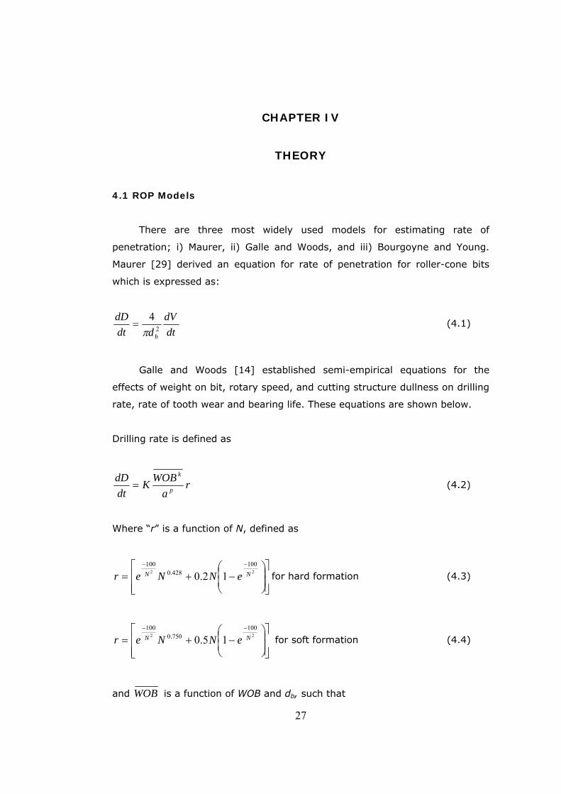
There are three most widely used models for estimating rate of
penetration; i) Maurer, ii) Galle and Woods, and iii) Bourgoyne and Young.
Maurer [29] derived an equation for rate of penetration for roller-cone bits
which is expressed as:
dtdV
ddtdD
b2
4π
= (4.1)
Galle and Woods [14] established semi-empirical equations for the
effects of weight on bit, rotary speed, and cutting structure dullness on drilling
rate, rate of tooth wear and bearing life. These equations are shown below.
Drilling rate is defined as
ra
WOBKdtdD
p
k
= (4.2)
Where “r” is a function of N, defined as
⎥⎥⎦
⎤
⎢⎢⎣
⎡⎟⎟⎠
⎞⎜⎜⎝
⎛−+=
−−22
100428.0
100
12.0 NN eNNer for hard formation (4.3)
⎥⎥⎦
⎤
⎢⎢⎣
⎡⎟⎟⎠
⎞⎜⎜⎝
⎛−+=
−−22
100750.0
100
15.0 NN eNNer for soft formation (4.4)
and WOB is a function of WOB and db, such that
27
bdWOBWOB 88.7
= (4.5)
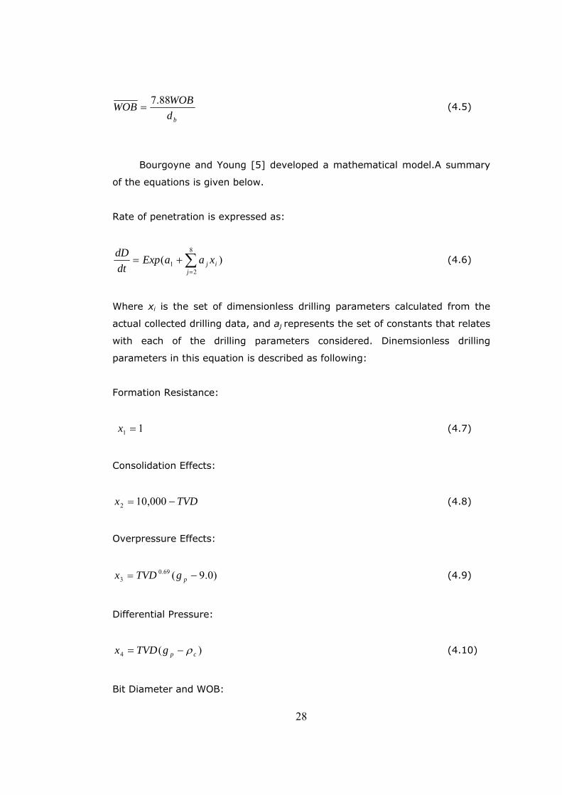
Bourgoyne and Young [5] developed a mathematical model.A summary
of the equations is given below.
Rate of penetration is expressed as:
∑=
+=8
21 )(
jij xaaExp
dtdD
(4.6)
Where xi is the set of dimensionless drilling parameters calculated from the
actual collected drilling data, and aj represents the set of constants that relates
with each of the drilling parameters considered. Dinemsionless drilling
parameters in this equation is described as following:
Formation Resistance:
(4.7) 11 =x
Consolidation Effects:
TVDx −= 000,102 (4.8)
Overpressure Effects:
)0.9(69.03 −= pgTVDx (4.9)
Differential Pressure:
)(4 cpgTVDx ρ−= (4.10)
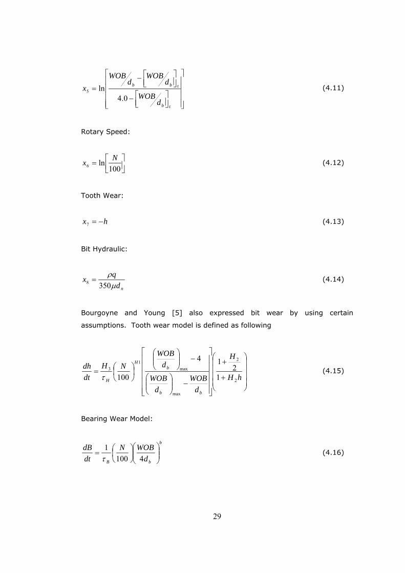
Bit Diameter and WOB:
28
⎥⎥⎥⎥
⎦
⎤
⎢⎢⎢⎢
⎣
⎡
⎥⎦⎤
⎢⎣⎡−
⎥⎦⎤
⎢⎣⎡−
=
tb
tbb
dWOB
dWOB
dWOB
x0.4
ln5 (4.11)
Rotary Speed:
⎥⎦⎤
⎢⎣⎡=100
ln6Nx (4.12)
Tooth Wear:
hx −=7 (4.13)
Bit Hydraulic:
ndqxμρ
3508 = (4.14)
Bourgoyne and Young [5] also expressed bit wear by using certain
assumptions. Tooth wear model is defined as following
⎟⎟⎟⎟
⎠
⎞
⎜⎜⎜⎜
⎝
⎛
+
+
⎥⎥⎥⎥⎥
⎦
⎤
⎢⎢⎢⎢⎢
⎣
⎡
−⎟⎟⎠
⎞⎜⎜⎝
⎛
−⎟⎟⎠
⎞⎜⎜⎝
⎛
⎟⎠⎞
⎜⎝⎛=
hH
H
dWOB
dWOB
dWOB
NHdtdh
bb
bH
H 2
2
max
max1
3
12
14
100τ (4.15)
Bearing Wear Model:
b
bB dWOBN
dtdB
⎟⎟⎠
⎞⎜⎜⎝
⎛⎟⎠⎞
⎜⎝⎛=
41001τ
(4.16)
29
4.2 Drilling Model
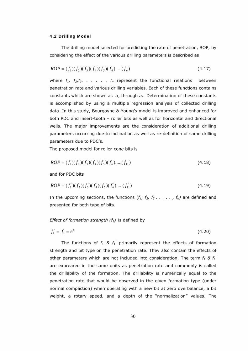
The drilling model selected for predicting the rate of penetration, ROP, by
considering the effect of the various drilling parameters is described as
)).....()()()()()(( 654321 nfffffffROP = (4.17)
where f1, f2,f3. . . . . . fn represent the functional relations between
penetration rate and various drilling variables. Each of these functions contains
constants which are shown as a1 through an. Determination of these constants
is accomplished by using a multiple regression analysis of collected drilling
data. In this study, Bourgoyne & Young’s model is improved and enhanced for
both PDC and insert-tooth – roller bits as well as for horizontal and directional
wells. The major improvements are the consideration of additional drilling
parameters occurring due to inclination as well as re-definition of same drilling
parameters due to PDC’s.
The proposed model for roller-cone bits is
)).....()()()()()(( 11654321 fffffffROP = (4.18)
and for PDC bits
)).....()()()()()(( '11
'6
'5
'4
'3
'2
'1 fffffffROP = (4.19)
In the upcoming sections, the functions (f1, f2, f3 . . . . . , fn) are defined and
presented for both type of bits.
Effect of formation strength (f1) is defined by
11
'1
aeff == (4.20)
The functions of f1 & f1’ primarily represent the effects of formation
strength and bit type on the penetration rate. They also contain the effects of
other parameters which are not included into consideration. The term f1 & f1’
are expreared in the same units as penetration rate and commonly is called
the drillability of the formation. The drillability is numerically equal to the
penetration rate that would be observed in the given formation type (under
normal compaction) when operating with a new bit at zero overbalance, a bit
weight, a rotary speed, and a depth of the “normalization” values. The
30
drillability of the various formations can be computed using drilling data
obtained from previous wells in the area.
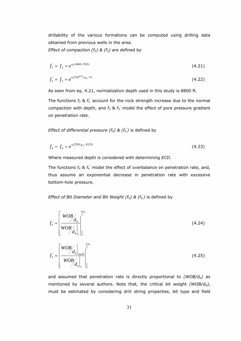
Effect of compaction (f2) & (f3) are defined by
)8800(
2'
22 TVDaeff −== (4.21)
)9(
3'
3
69.03 −== pgTVDaeff (4.22)
As seen from eq. 4.21, normalization depth used in this study is 8800 ft. The functions f2 & f2’ account for the rock strength increase due to the normal
compaction with depth, and f3 & f3’ model the effect of pore pressure gradient
on penetration rate.
Effect of differential pressure (f4) & (f4’) is defined by
)(
4'
44 ECDgTVDa peff −== (4.23)
Where measured depth is considered with determining ECD. The functions f4 & f4’ model the effect of overbalance on penetration rate, and,
thus assume an exponential decrease in penetration rate with excessive
bottom-hole pressure.
Effect of Bit Diameter and Bit Weight (f5) & (f5’) is defined by
5
5
a
cb
b
dWOB
dWOB
f
⎥⎥⎥⎥
⎦
⎤
⎢⎢⎢⎢
⎣
⎡
= (4.24)
5
'5
a
cb
mechb
dWOB
dWOB
f
⎥⎥⎥⎥
⎦
⎤
⎢⎢⎢⎢
⎣
⎡
= (4.25)
and assumed that penetration rate is directly proportional to (WOB/db) as
mentioned by several authors. Note that, the critical bit weight (WOB/db)c
must be estimated by considering drill string properties, bit type and field
31
data. In this study, normalization value for critical bit weight is assumed to be
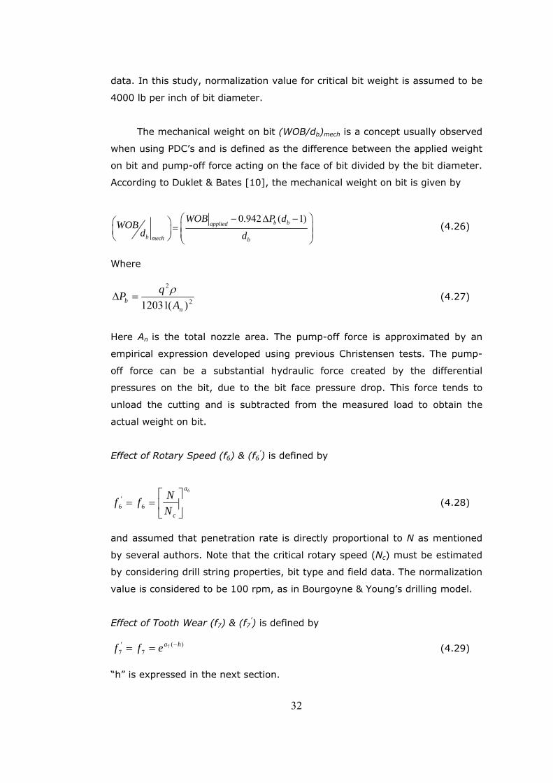
4000 lb per inch of bit diameter.
The mechanical weight on bit (WOB/db)mech is a concept usually observed
when using PDC’s and is defined as the difference between the applied weight
on bit and pump-off force acting on the face of bit divided by the bit diameter.
According to Duklet & Bates [10], the mechanical weight on bit is given by
0.942 ( 1)b bapplied
b mech b
WOB P dWOBd d
⎛ − Δ⎛ ⎞ = ⎜⎜ ⎟ ⎜ ⎟⎝ ⎠ ⎝ ⎠
− ⎞⎟ (4.26)
Where
2
2
)(12031 nb A
qP ρ=Δ (4.27)
Here An is the total nozzle area. The pump-off force is approximated by an
empirical expression developed using previous Christensen tests. The pump-
off force can be a substantial hydraulic force created by the differential
pressures on the bit, due to the bit face pressure drop. This force tends to
unload the cutting and is subtracted from the measured load to obtain the
actual weight on bit.
Effect of Rotary Speed (f6) & (f6’) is defined by
6
6'
6
a
cNNff ⎥⎦
⎤⎢⎣
⎡== (4.28)
and assumed that penetration rate is directly proportional to N as mentioned
by several authors. Note that the critical rotary speed (Nc) must be estimated
by considering drill string properties, bit type and field data. The normalization
value is considered to be 100 rpm, as in Bourgoyne & Young’s drilling model.
Effect of Tooth Wear (f7) & (f7’) is defined by
)(7
'7
7 haeff −== (4.29) “h” is expressed in the next section.
32
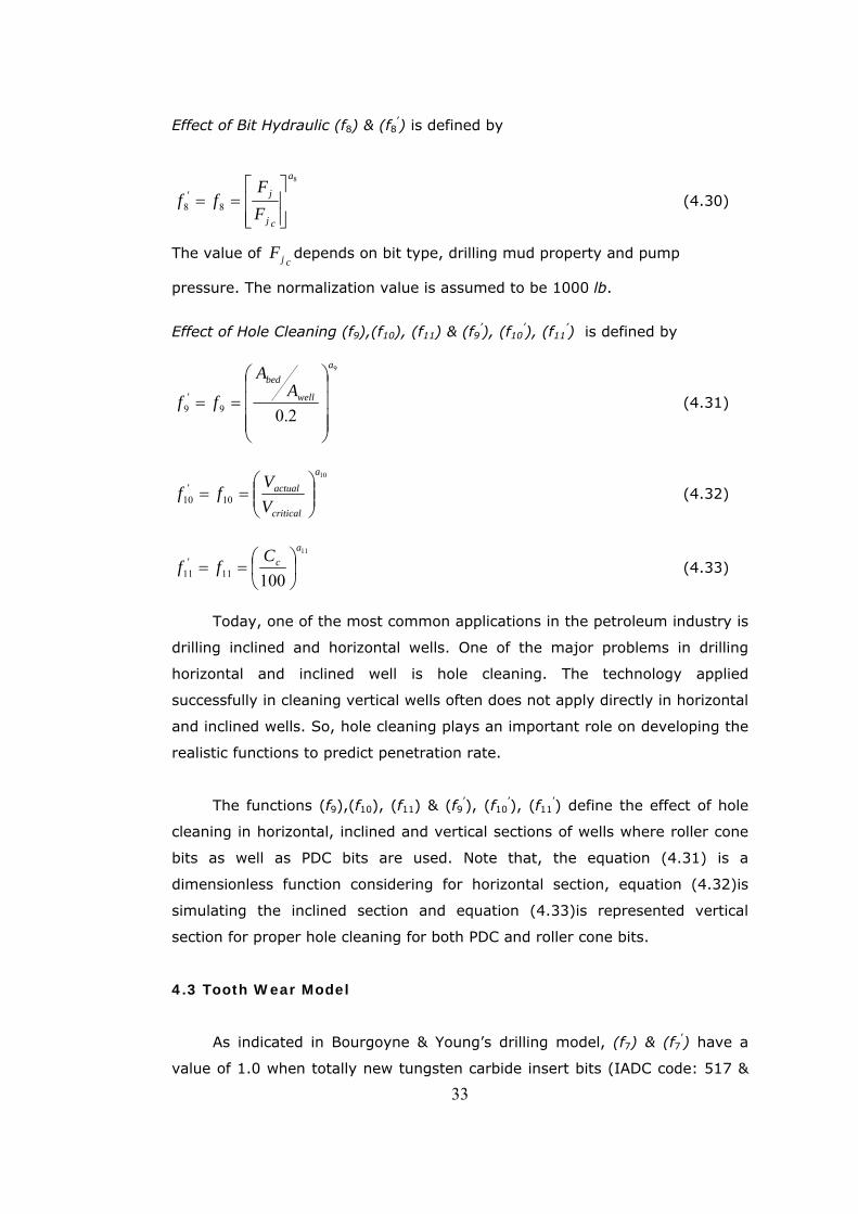
Effect of Bit Hydraulic (f8) & (f8’) is defined by
8
8'
8
a
cj
j
FF
ff⎥⎥⎦
⎤
⎢⎢⎣
⎡== (4.30)
The value of depends on bit type, drilling mud property and pump
pressure. The normalization value is assumed to be 1000 lb.
cjF
Effect of Hole Cleaning (f9),(f10), (f11) & (f9’), (f10
’), (f11’) is defined by
9
2.09'
9
a
well
bedA
A
ff⎟⎟⎟⎟
⎠
⎞
⎜⎜⎜⎜
⎝
⎛
== (4.31)
10
10'
10
a
critical
actual
VV
ff ⎟⎟⎠
⎞⎜⎜⎝
⎛== (4.32)
11
10011'
11
acC
ff ⎟⎠⎞
⎜⎝⎛== (4.33)
Today, one of the most common applications in the petroleum industry is
drilling inclined and horizontal wells. One of the major problems in drilling
horizontal and inclined well is hole cleaning. The technology applied
successfully in cleaning vertical wells often does not apply directly in horizontal
and inclined wells. So, hole cleaning plays an important role on developing the
realistic functions to predict penetration rate.
The functions (f9),(f10), (f11) & (f9’), (f10’), (f11
’) define the effect of hole
cleaning in horizontal, inclined and vertical sections of wells where roller cone
bits as well as PDC bits are used. Note that, the equation (4.31) is a
dimensionless function considering for horizontal section, equation (4.32)is
simulating the inclined section and equation (4.33)is represented vertical
section for proper hole cleaning for both PDC and roller cone bits.
4.3 Tooth Wear Model
As indicated in Bourgoyne & Young’s drilling model, (f7) & (f7’) have a
value of 1.0 when totally new tungsten carbide insert bits (IADC code: 517 &
33
523) and PDC bits are used. In this study, it is assumed that bit cone offset
selection is proper. So bearing wear is negligible. The developed model for
estimating frictional tooth dullness, h, is given by
))()()(( 4321 ggggdtdh
= (4.34)
The function g1 describes the effect of formation abrasiveness on tooth wear
and defined by
H
Hg
τ3
1 = (4.35)
In equation (4.35), the value of H3 for tungsten carbide insert bits (IADC
code: 517 & 523) and PDC bits is 0.02 according to Bourgoyne and Young
and the value of τH depend on formation properties and it must be estimated
using drill-off tests or previously drilled well data. The function g2 considers
the effect of weight on bit on tooth wear. This function is different for tungsten
carbide insert bits (IADC code: 517 & 523) and PDC’s. For tungsten carbide
insert bits (IADC code: 517 & 523) it is defined by
⎥⎥⎥⎥
⎦
⎤
⎢⎢⎢⎢
⎣
⎡
−⎟⎠⎞⎜
⎝⎛
−⎟⎠⎞⎜
⎝⎛
=
bb
b
dWOB
dWOB
dWOB
g
max
max2
9.2 (4.36)
Estes [57] has pointed out that the rate of bit wear will be excessive if a very
high bit weight is used. His recommended maximum bit weights were used in
this study. For PDC bits, the effect of weight on bit on tooth wear is defined by
⎥⎥⎥⎥
⎦
⎤
⎢⎢⎢⎢
⎣
⎡
=
mechb
cirb
dWOB
dWOB
g 2 (4.37)
Note that the normalized bit weight (WOB/db )cir must be estimated by
considering drill string properties, bit type and field data. In this study, the
normalization value is assumed as 100 lb per inch of bit diameter.
34
The function g3 describes the effect of pipe rotation on tooth wear and
defined by
1
3
H
cNNg ⎥⎦
⎤⎢⎣
⎡= (4.38)
The value of H1 for tungsten carbide insert bits (IADC code: 517 & 523) and
PDC bits is 1.50 according to Bourgoyne & Young and the value of Nc depend
on drill string properties and bit type.
The function g4 is used to emphasize the effect of tooth geometry on
tooth wear. For all types of bits, tooth wear is proportional to the inverse of
the contact area (A) if failing by fracturing of brittle tungsten carbide is
ignored. Generally the shape of bits should be classified into three main
shapes: cylindrical, triangular and spherical. For cylindrical shape, since there
is no change in contact area, the effect of tooth geometry on tooth wear is
given by
14 =g (4.39) For triangular shape, the effect of tooth geometry on tooth wear is given by
⎟⎟⎟
⎠
⎞
⎜⎜⎜
⎝
⎛
+
+=
hH
Hg
2
2
4 121
(4.40)
The value of H2 is 1.0 according to Bourgoyne & Young. Finally, for spherical
shape, the effect of tooth geometry on tooth wear is given by
⎟⎟⎠
⎞⎜⎜⎝
⎛
−=
)2(1
4 hhdg
c
(4.41)
By substituting equations (4.35 through 4.41) into equation (4.34) and
integrating for h, the value of frictional tooth dullness, h, can be calculated.
35
4.4 CUTTINGS TRANSPORT
One of the primary functions of drilling fluids in rotary drilling is to
remove the rock fragments from beneath the bit and transport these cuttings
to the surface. Insufficient hole cleaning cause enormous drilling problems,
those may result in losing the overall well.
4.4.1 Vertical Wells
As a rule of thumb, from experiences, average cuttings concentration
should not exceed 5 % in the annulus for vertical wells. [6] Therefore, flow
rates required can be determined by using this criterion. An equation for the
volumetric cuttings concentration, Cc, can be derived on the basis of mass
balance. After simplification and in field units, volumetric cuttings
concentration can be derived as
Qvv
DROPC
f
s
bc
⎟⎟⎠
⎞⎜⎜⎝
⎛−
=
195.1466
)( 2
(4.42)
In order for the fluid to lift the cuttings to the surface, the fluid annular
velocity, vf, should be higher than cuttings slip velocity, vs.
vf can be written as
)(4
22io
f
DD
Qv−
=π
(4.43)
4.4.2 Inclined and Horizontal Wells
The transport of cuttings for inclined and horizontal wells is much more
complicated than it is for vertical wells. There are two major problems that are
not present in vertical wells. One problem is the existence and thickness of a
bed of cuttings on the low side of the hole. The other problem is the sliding
and/or saltating cuttings within the hole. At angles of inclination around 40o-
36
60o, the bed of cuttings has the tendency to backslide, and the bed is said to
be unstable. Having an unstable bed places the drill string in risk and
especially so any time mud circulation is halted.
4.4.3 The Dimensionless Analysis to calculate Cc, Abed/Awell &
Vactual/Vcritical
During the determination of rate of penetration constants different
correlation are used to different inclination. For vertical and close to vertical
inclinations equation (4.42), for higher inclinations up to 60 o calculation of
critical annular fluid velocity model and for inclination grater than 60o and
horizontal section Ozbayoglu’s cutting bed estimation model is selected. The
results obtained from these equations was assumed as observed data.The
major aspects of average volumetric cuttings concentration method,
calculation of critical annular fluid velocity and cuttings concentration and
Ozbayoglu’s model are presented in appendix B.
With in the proper model for estimating rate of penetration, the following
general and dimensionless equations for different inclination are selected by
considering the effects of the four independent variables on cutting transport
and hole cleaning.These variables namely are flow rate, hole angle, cuttings
size and pipe rotation.[32]
For vertical section )100( ≤≤ θ
564321 ))1091(tanh( a
aaa
dca
rc TRFaC −×−= θ (4.44) For inclined section )6010( ≤≤ θ
564321 ))1091(tanh( b
abb
dcb
rcritical
actual TRFbVV −×−= θ (4.45)
For horizontal section )9060( ≤≤ θ
654321
cs
ccr
cr
cre
well
bed SAFNcAA θ= (4.46)
By using these equations, Cc, Abed/Awell and Vactual/Vcritical are calculated in order
to predict ROP by using proposed model.
37
4.5 OPTIMIZATION OF THE PENETRATION RATE
The drilling optimization procedure considered in this study, is based on
two objective functions i) maximizing the rate of penetration, and ii)
minimizing cost per foot. In order to derive the optimum drilling parameters
analytically, two separate differential equations are definded i) rate of
penetration (eq 4.48) and ii) teeth wear as a function of time (eq 4.49). In a
general form, they can be written as:
),,/(1 hNdWOBfdtdDROP b== (4.48)
),,/(2 hNdWOBfdtdh
b= (4.49)
As seen in equations (4.48) & (4.49), only the operable parameters can be
considered. So, it can be concluded that drilling optimization can be conducted
to select the proper weight on bit and rotary speed. During analytical
derivation of optimum value for weight on bit and rotary speed, some
constraints due to practical application are introduced.
maxmin WOBWOBWOB ≤≤ (4.50)
maxmin NNN ≤≤ (4.51)
(4.52) 0.10 ≤≤ h
Where for totally worn out teeth, the value of h is zero and for new teeth, it
equal to one.
As mentioned earlier, bearing wear is ignored. So it can be considered
that only, tooth wear limits bit life. The drilling cost per foot equation is given
by
38
DtttCC
C bctrbf Δ
+++=
)( (4.53)
The above equation can be rearranged to give
⎟⎟⎠
⎞⎜⎜⎝
⎛+++
Δ= bct
r
brf ttt
CC
DC
C (4.54)
From the equation (4.34), for insert roller cone bit
⎟⎟⎟
⎠
⎞
⎜⎜⎜
⎝
⎛
+⎥⎦⎤
⎢⎣⎡
⎥⎥⎥⎥
⎦
⎤
⎢⎢⎢⎢
⎣
⎡
−⎟⎠⎞⎜
⎝⎛
−⎟⎠⎞⎜
⎝⎛
=
21
1
9.2 2
max
max
32
1
HNN
dWOB
dWOB
dWOB
HJ
Hc
b
bbHτ (4.55)
By using the equations (4.48), (4.49) and (4.55), rotating time during bit run
and footage drilled can be determined for insert roller cone bit.
)2/()1( 222
022 ff
h
b hHhJdhhHJtf
+=+= ∫ (4.56)
From the equation (4.34), for PDC bits
⎟⎟⎟
⎠
⎞
⎜⎜⎜
⎝
⎛
+⎥⎦⎤
⎢⎣⎡
⎥⎥⎥⎥
⎦
⎤
⎢⎢⎢⎢
⎣
⎡
=
21
123
'2
1
HNN
dWOB
dWOB
HJ
Hc
cirb
mechbHτ (4.57)
By using the equations (4.48), (4.49) and (4.57), rotating time during bit run
and footage drilled can be determined for PDC bit.
)2/()1( 22
'2
02
'2 ff
h
b hHhJdhhHJtf
+=+= ∫ (4.58)
39
Composite drilling variables J1 and J1’ are defined by using the equations
(4.18) and (4.19).
))()()()()()()()()(( 1110986543211 ffffffffffJ = (4.59)
))()()()()()()()()(( '11
'10
'9
'8
'6
'5
'4
'3
'2
'1
'1 ffffffffffJ = (4.60)
So, the equation (4.48) can be re-writen as below:
For tungsten carbide insert bits
haeJfJdtdD
7171
−== (4.61)
For PDC bits
haeJfJdtdD
7'17
'1
−== (4.62)
Separating variables in these equations yield.
For tungsten carbide insert bits
dteJdD ha71
−= (4.63)
For PDC bits
dteJdD ha7'1
−= (4.64)
The integration of these equations requires a relation between time t and
tooth wear h. by recall equations (4.34), (4.55) and (4.57) and substitut these
expressions into equations. (4.63)& (4.64), respectively
40
For tungsten carbide insert bits
dhhHeJJdD ha )1( 2127 += − (4.65)
For PDC bits
dhhHeJJdD ha )1( 2'1
'2
7 += − (4.66)
If both side of equations (4.65) & (4.66) are integrated,the following equations
can be derived as function of final tooth wear during a corresponding footage.
For tungsten carbide insert bits
⎥⎥⎦
⎤
⎢⎢⎣
⎡ −−+
−=Δ
−−−
27
72
712
)1(1 777
aehaeH
aeJJD
fffha
fhaha
(4.67)
For PDC bits
⎥⎥⎦
⎤
⎢⎢⎣
⎡ −−+
−=Δ
−−−
27
72
7
'1
'2
)1(1 777
aehaeH
aeJJD
fffha
fhaha
(4.68)
After defining footage, substituting equations (4.67) & (4.68) and equations
(4.56) & (4.58) into cost per foot equation (4.54), the cost per foot equation
can be expressed as following:
For tungsten carbide insert bits
⎥⎥⎥⎥⎥
⎦
⎤
⎢⎢⎢⎢⎢
⎣
⎡+
+++
+
=∫
∫ − 1
02
21
02
)1(
)1(7J
dhhH
JJ
ttCC
dhhHe
CC
f
f
h
ctr
b
hha
rf (4.69)
41
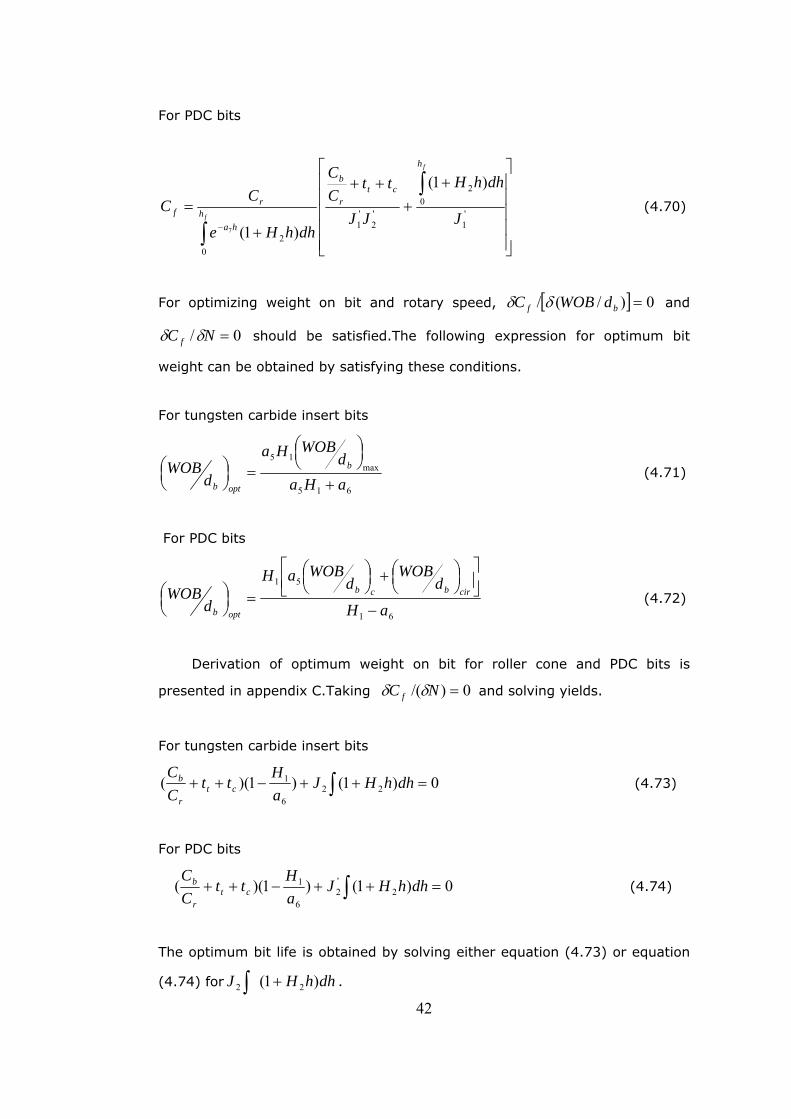
For PDC bits
⎥⎥⎥⎥⎥
⎦
⎤
⎢⎢⎢⎢⎢
⎣
⎡+
+++
+
=∫
∫ −'1
02
'2
'1
02
)1(
)1(7J
dhhH
JJ
ttCC
dhhHe
CC
f
f
h
ctr
b
hha
rf (4.70)
For optimizing weight on bit and rotary speed, [ ] 0)/(/ =bf dWOBC δδ and
0/ =NC f δδ should be satisfied.The following expression for optimum bit
weight can be obtained by satisfying these conditions.
For tungsten carbide insert bits
615
max15
aHad
WOBHa
dWOB b
optb +
⎟⎠⎞⎜
⎝⎛
=⎟⎠⎞⎜
⎝⎛ (4.71)
For PDC bits
61
51
aH
dWOB
dWOBaH
dWOB cirbcb
optb −
⎥⎦⎤
⎢⎣⎡
⎟⎠⎞⎜
⎝⎛+⎟
⎠⎞⎜
⎝⎛
=⎟⎠⎞⎜
⎝⎛ (4.72)
Derivation of optimum weight on bit for roller cone and PDC bits is
presented in appendix C.Taking 0)/( =NC f δδ and solving yields.
For tungsten carbide insert bits
0)1()1)(( 226
1 =++−++ ∫ dhhHJaHtt
CC
ctr
b (4.73)
For PDC bits
0)1()1)(( 2'2
6
1 =++−++ ∫ dhhHJaHtt
CC
ctr
b (4.74)
The optimum bit life is obtained by solving either equation (4.73) or equation
(4.74) for dhhHJ )1( 22 +∫ .
42
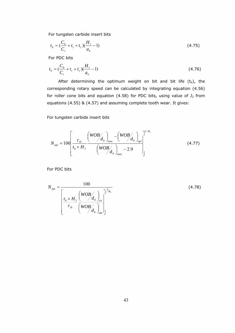
For tungsten carbide insert bits
)1)((6
1 −++=aHtt
CC
t ctr
bb (4.75)
For PDC bits
)1)((6
1 −++=aHtt
CC
t ctr
bb (4.76)
After determining the optimum weight on bit and bit life (tb), the
corresponding rotary speed can be calculated by integrating equation (4.56)
for roller cone bits and equation (4.58) for PDC bits, using value of J2 from
equations (4.55) & (4.57) and assuming complete tooth wear. It gives:
For tungsten carbide insert bits
1/1
max
max
3 9.2100
H
b
optbb
b
Hopt
dWOB
dWOB
dWOB
HtN
⎥⎥⎥⎥
⎦
⎤
⎢⎢⎢⎢
⎣
⎡
−⎟⎠⎞⎜
⎝⎛
⎟⎠⎞⎜
⎝⎛−⎟
⎠⎞⎜
⎝⎛
×=
τ (4.77)
For PDC bits
11
3
100H
optb
cirb
H
b
opt
dWOB
dWOB
Ht
N
⎥⎥⎥⎥
⎦
⎤
⎢⎢⎢⎢
⎣
⎡
⎟⎠⎞⎜
⎝⎛
⎟⎠⎞⎜
⎝⎛
×
=
τ
(4.78)
43
44
CHAPTER V
DEVELOPMENT OF THE PROPOSED MODEL
A rate of penetration model is developed by considering many drilling
parameters.The model can be used for horizontal and inclined wells with roller
cone and PDC bits.Using the data provided from wells drilled at Persian Gulf,
model parameters could be determined.Then, optimum weight and rotary
speed is derived analiticaly using the proposed model.
5.1 Selecting and sorting relevant and proper field data
An Excel program has been provided to identify and store the field data.
In this program firstly, data which were obtained from different wells and
formations, were rearranged and then normalized by dividing them to their
normalized value.These data which included depth, rate of penetration, weight
on bit, drilling rotating time, flow rate, nozzles diameter, mud weight, pore
pressure and pump pressure Sorted according to the IADC code, the bit
diameter and formation type. This program also determines bit hydraulic
information, bit wear condition, and hole cleaning performance. Finally, a data
file created which can be used in multiple regression analysis.
5.2 Regression Analysis
A computer program has been developed to determine the coefficients of
the proposed rate of penetration model using Multiple Regression Technique.
The idea of using a regression analysis of past drilling data to evaluate
constants in a drilling rate equation is known. However, most of the past work
in this area has been hampered because obtaining large volumes of accurate
field data were difficult and the effects of many of the drilling parameters
discussed in section (4.2) were ignored. A derivation of the multiple
regression-analysis procedure is presented in detail in appendix A.
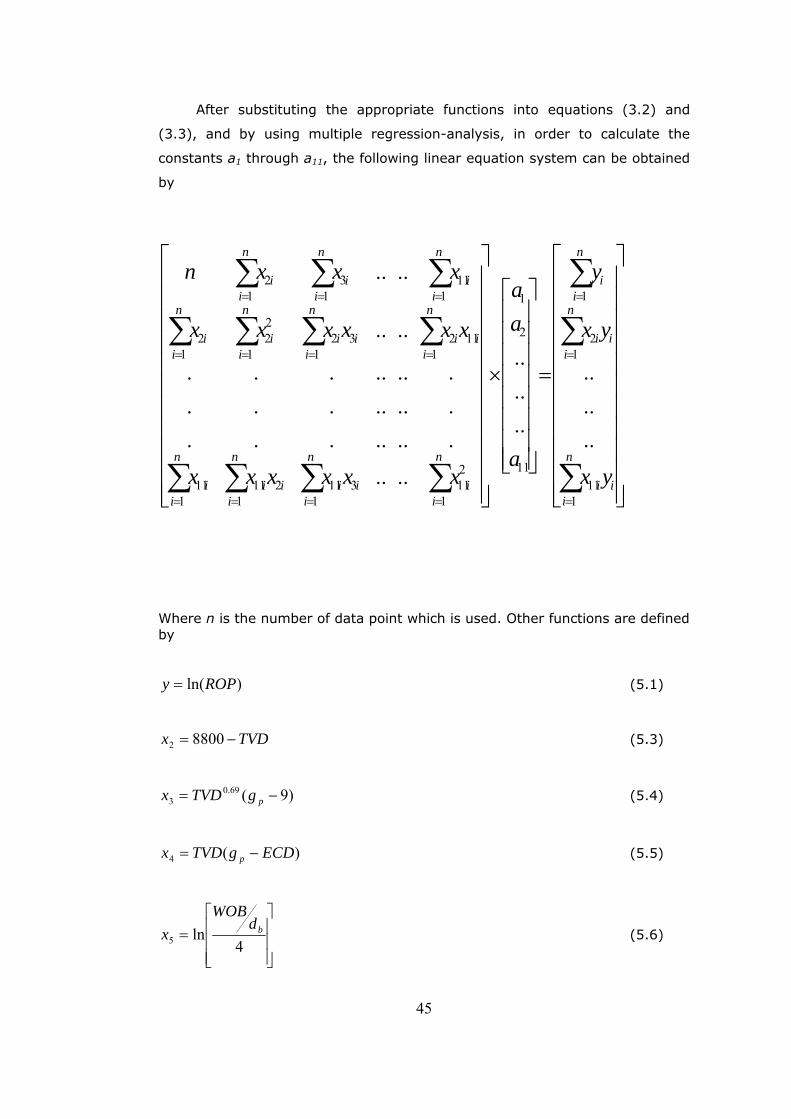
After substituting the appropriate functions into equations (3.2) and
(3.3), and by using multiple regression-analysis, in order to calculate the
constants a1 through a11, the following linear equation system can be obtained
by
⎥⎥⎥⎥⎥⎥⎥⎥⎥⎥⎥
⎦
⎤
⎢⎢⎢⎢⎢⎢⎢⎢⎢⎢⎢
⎣
⎡
=
⎥⎥⎥⎥⎥⎥⎥⎥
⎦
⎤
⎢⎢⎢⎢⎢⎢⎢⎢
⎣
⎡
×
⎥⎥⎥⎥⎥⎥⎥⎥⎥⎥⎥
⎦
⎤
⎢⎢⎢⎢⎢⎢⎢⎢⎢⎢⎢
⎣
⎡
∑
∑
∑
∑∑∑∑
∑∑∑∑
∑∑∑
=
=
=
====
====
===
n
iii
n
iii
n
ii
n
ii
n
iii
n
iii
n
ii
n
iii
n
iii
n
ii
n
ii
n
ii
n
ii
n
ii
yx
yx
y
a
aa
xxxxxx
xxxxxx
xxxn
111
12
1
11
2
1
1
211
1311
1211
111
1112
132
1
22
12
111
13
12
..
..
..
..
..
..
............................
....
....
Where n is the number of data point which is used. Other functions are defined by
)ln(ROPy = (5.1)
TVDx −= 88002 (5.3)
)9(69.03 −= pgTVDx (5.4)
)(4 ECDgTVDx p −= (5.5)
⎥⎥⎥
⎦
⎤
⎢⎢⎢
⎣
⎡=
4ln5
bdWOB
x (5.6)
45
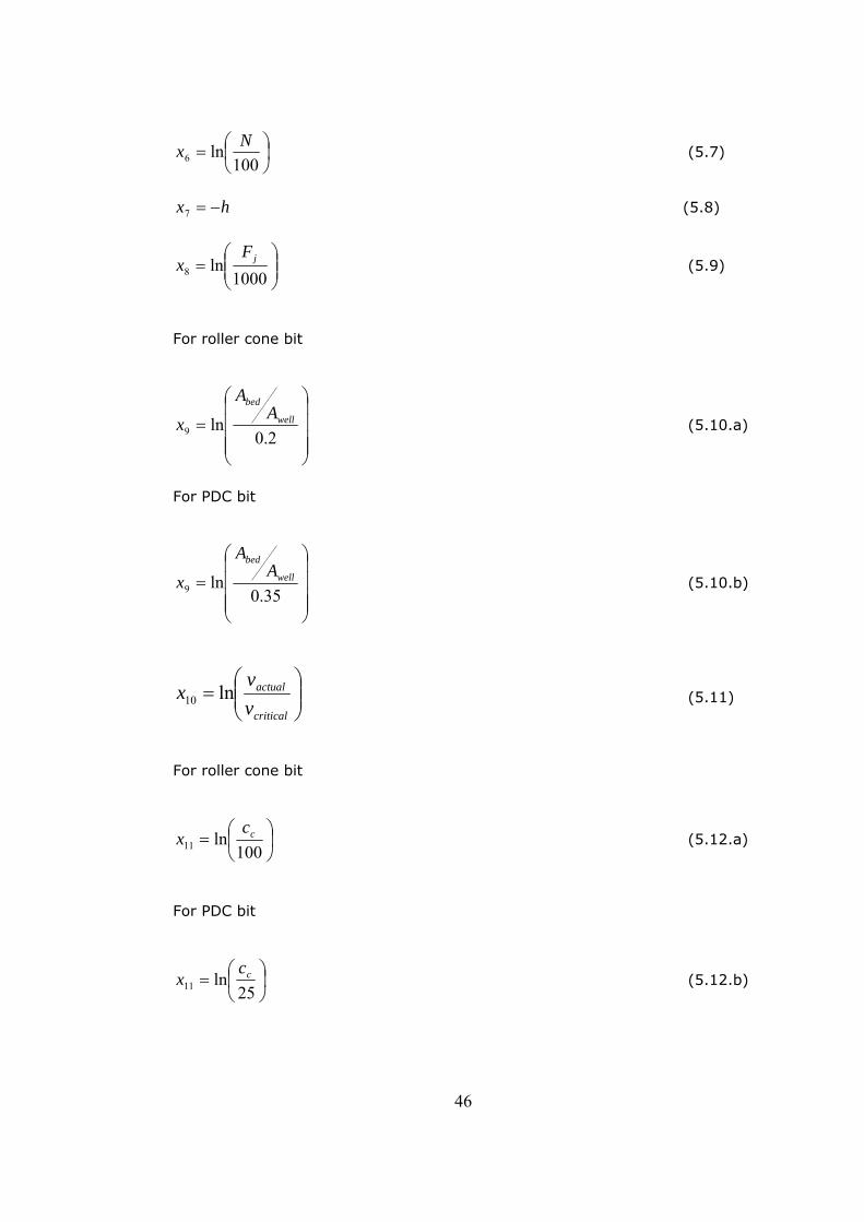
⎟⎠⎞
⎜⎝⎛=100
ln6Nx (5.7)
hx −=7 (5.8)
⎟⎟⎠
⎞⎜⎜⎝
⎛=
1000ln8
jFx (5.9)
For roller cone bit
⎟⎟⎟⎟
⎠
⎞
⎜⎜⎜⎜
⎝
⎛
=2.0
ln9well
bedA
A
x (5.10.a)
For PDC bit
⎟⎟⎟⎟
⎠
⎞
⎜⎜⎜⎜
⎝
⎛
=35.0
ln9well
bedA
A
x (5.10.b)
⎟⎟⎠
⎞⎜⎜⎝
⎛=
critical
actual
vv
x ln10 (5.11)
For roller cone bit
⎟⎠⎞
⎜⎝⎛=100
ln11cc
x (5.12.a)
For PDC bit
⎟⎠⎞
⎜⎝⎛=
25ln11
ccx (5.12.b)
46
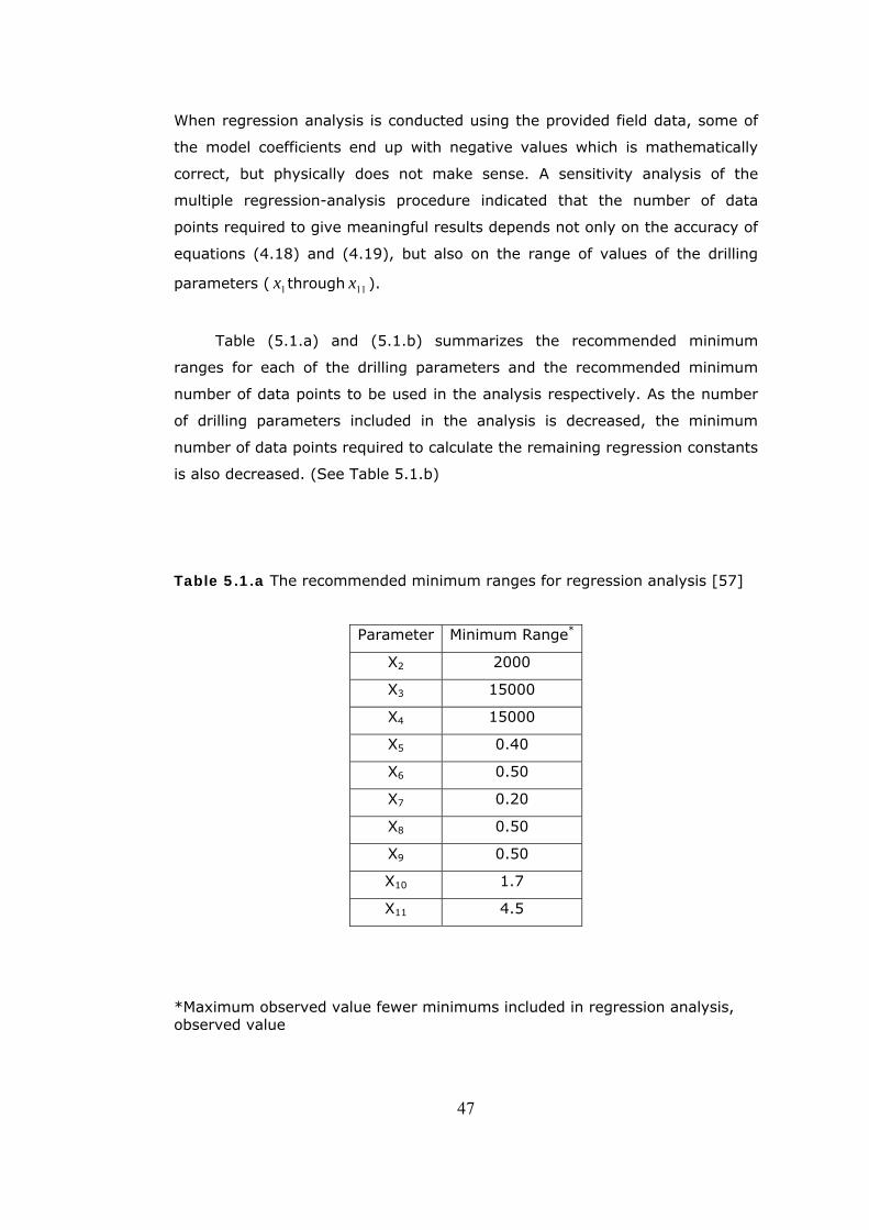
When regression analysis is conducted using the provided field data, some of
the model coefficients end up with negative values which is mathematically
correct, but physically does not make sense. A sensitivity analysis of the
multiple regression-analysis procedure indicated that the number of data
points required to give meaningful results depends not only on the accuracy of
equations (4.18) and (4.19), but also on the range of values of the drilling
parameters ( through ). 1x 11x
Table (5.1.a) and (5.1.b) summarizes the recommended minimum
ranges for each of the drilling parameters and the recommended minimum
number of data points to be used in the analysis respectively. As the number
of drilling parameters included in the analysis is decreased, the minimum
number of data points required to calculate the remaining regression constants
is also decreased. (See Table 5.1.b)
Table 5.1.a The recommended minimum ranges for regression analysis [57]
Parameter Minimum Range*
X2 2000
X3 15000
X4 15000
X5 0.40
X6 0.50
X7 0.20
X8 0.50
X9 0.50
X10 1.7
X11 4.5
*Maximum observed value fewer minimums included in regression analysis, observed value
47
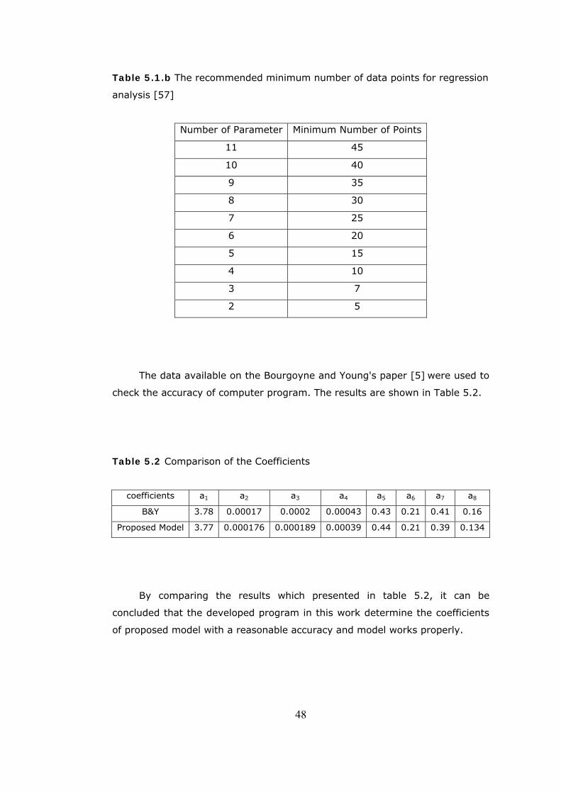
48
Table 5.1.b The recommended minimum number of data points for regression
analysis [57]
Number of Parameter Minimum Number of Points
11 45
10 40
9 35
8 30
7 25
6 20
5 15
4 10
3 7
2 5
The data available on the Bourgoyne and Young's paper [5] were used to
check the accuracy of computer program. The results are shown in Table 5.2.
Table 5.2 Comparison of the Coefficients
coefficients a1 a2 a3 a4 a5 a6 a7 a8
B&Y 3.78 0.00017 0.0002 0.00043 0.43 0.21 0.41 0.16
Proposed Model 3.77 0.000176 0.000189 0.00039 0.44 0.21 0.39 0.134
By comparing the results which presented in table 5.2, it can be
concluded that the developed program in this work determine the coefficients
of proposed model with a reasonable accuracy and model works properly.
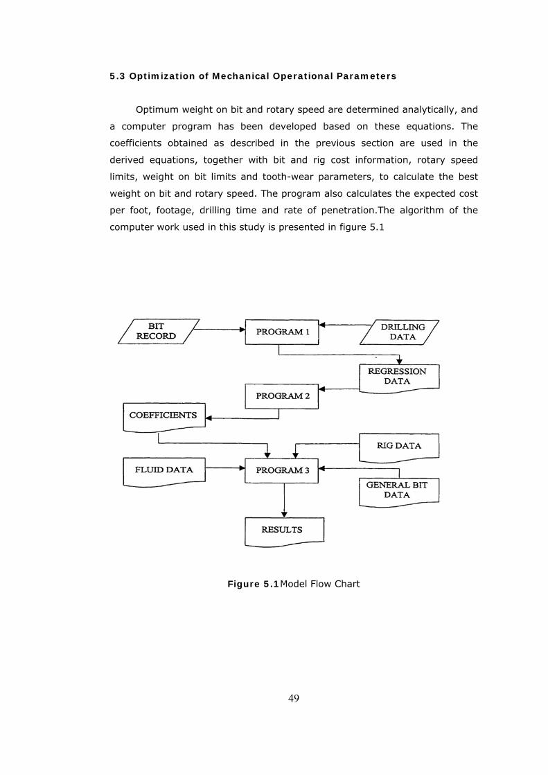
5.3 Optimization of Mechanical Operational Parameters
Optimum weight on bit and rotary speed are determined analytically, and
a computer program has been developed based on these equations. The
coefficients obtained as described in the previous section are used in the
derived equations, together with bit and rig cost information, rotary speed
limits, weight on bit limits and tooth-wear parameters, to calculate the best
weight on bit and rotary speed. The program also calculates the expected cost
per foot, footage, drilling time and rate of penetration.The algorithm of the
computer work used in this study is presented in figure 5.1
Figure 5.1Model Flow Chart
49
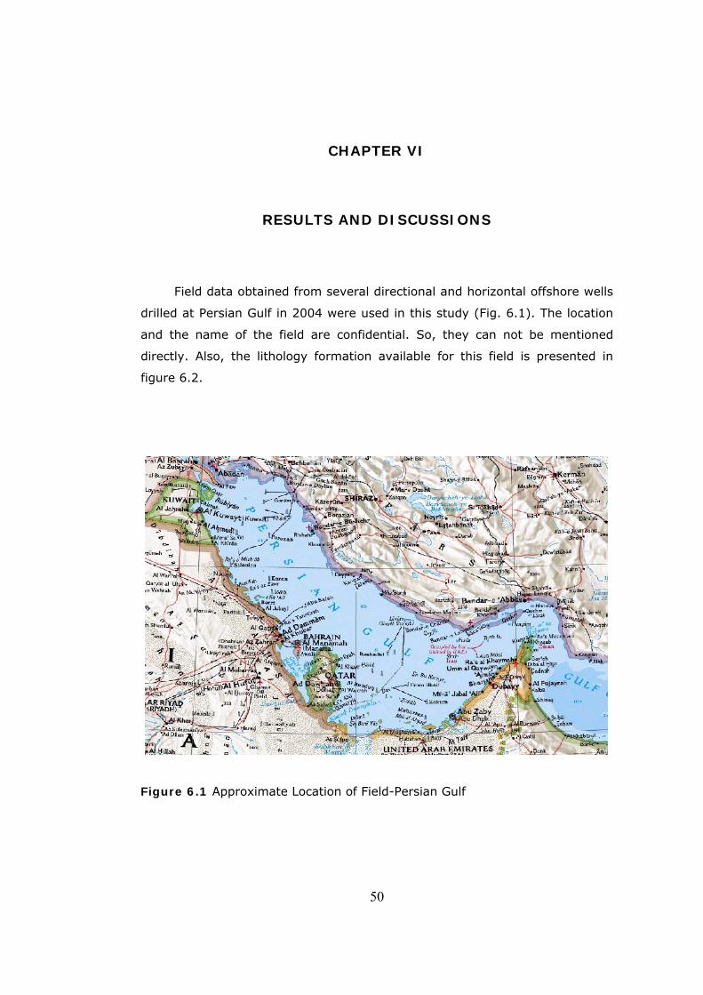
CHAPTER VI
RESULTS AND DISCUSSIONS
Field data obtained from several directional and horizontal offshore wells
drilled at Persian Gulf in 2004 were used in this study (Fig. 6.1). The location
and the name of the field are confidential. So, they can not be mentioned
directly. Also, the lithology formation available for this field is presented in
figure 6.2.
Figure 6.1 Approximate Location of Field-Persian Gulf
50
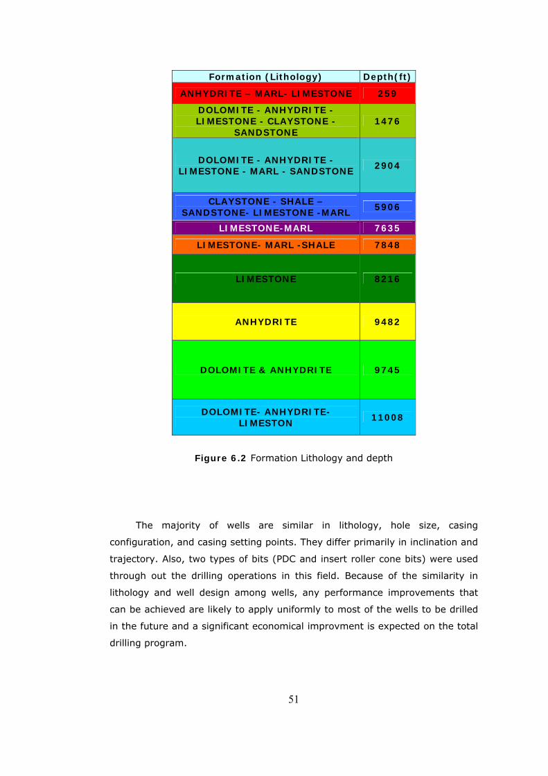
51
Formation (Lithology) Depth(ft)
ANHYDRITE – MARL- LIMESTONE 259
DOLOMITE - ANHYDRITE - LIMESTONE - CLAYSTONE -
SANDSTONE 1476
DOLOMITE - ANHYDRITE - LIMESTONE - MARL - SANDSTONE 2904
CLAYSTONE - SHALE – SANDSTONE- LIMESTONE -MARL 5906
LIMESTONE-MARL 7635
LIMESTONE- MARL -SHALE 7848
LIMESTONE 8216
ANHYDRITE 9482
DOLOMITE & ANHYDRITE 9745
DOLOMITE- ANHYDRITE-LIMESTON 11008
Figure 6.2 Formation Lithology and depth
The majority of wells are similar in lithology, hole size, casing
configuration, and casing setting points. They differ primarily in inclination and
trajectory. Also, two types of bits (PDC and insert roller cone bits) were used
through out the drilling operations in this field. Because of the similarity in
lithology and well design among wells, any performance improvements that
can be achieved are likely to apply uniformly to most of the wells to be drilled
in the future and a significant economical improvment is expected on the total
drilling program.
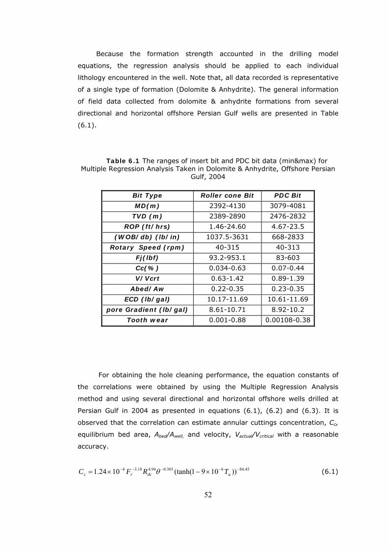
Because the formation strength accounted in the drilling model
equations, the regression analysis should be applied to each individual
lithology encountered in the well. Note that, all data recorded is representative
of a single type of formation (Dolomite & Anhydrite). The general information
of field data collected from dolomite & anhydrite formations from several
directional and horizontal offshore Persian Gulf wells are presented in Table
(6.1).
Table 6.1 The ranges of insert bit and PDC bit data (min&max) for Multiple Regression Analysis Taken in Dolomite & Anhydrite, Offshore Persian
Gulf, 2004
Bit Type Roller cone Bit PDC Bit MD(m) 2392-4130 3079-4081
TVD (m) 2389-2890 2476-2832 ROP (ft/hrs) 1.46-24.60 4.67-23.5
(WOB/db) (lb/in) 1037.5-3631 668-2833 Rotary Speed (rpm) 40-315 40-313
Fj(lbf) 93.2-953.1 83-603 Cc(%) 0.034-0.63 0.07-0.44 V/Vcrt 0.63-1.42 0.89-1.39
Abed/Aw 0.22-0.35 0.23-0.35 ECD (lb/gal) 10.17-11.69 10.61-11.69
pore Gradient (lb/gal) 8.61-10.71 8.92-10.2 Tooth wear 0.001-0.88 0.00108-0.38
For obtaining the hole cleaning performance, the equation constants of
the correlations were obtained by using the Multiple Regression Analysis
method and using several directional and horizontal offshore wells drilled at
Persian Gulf in 2004 as presented in equations (6.1), (6.2) and (6.3). It is
observed that the correlation can estimate annular cuttings concentration, Cc,
equilibrium bed area, Abed/Awell, and velocity, Vactual/Vcritical with a reasonable
accuracy.
45.846303.094.418.34 ))1091(tanh(1024.1 −−−−− ×−×= adcrc TRFC θ (6.1)
52
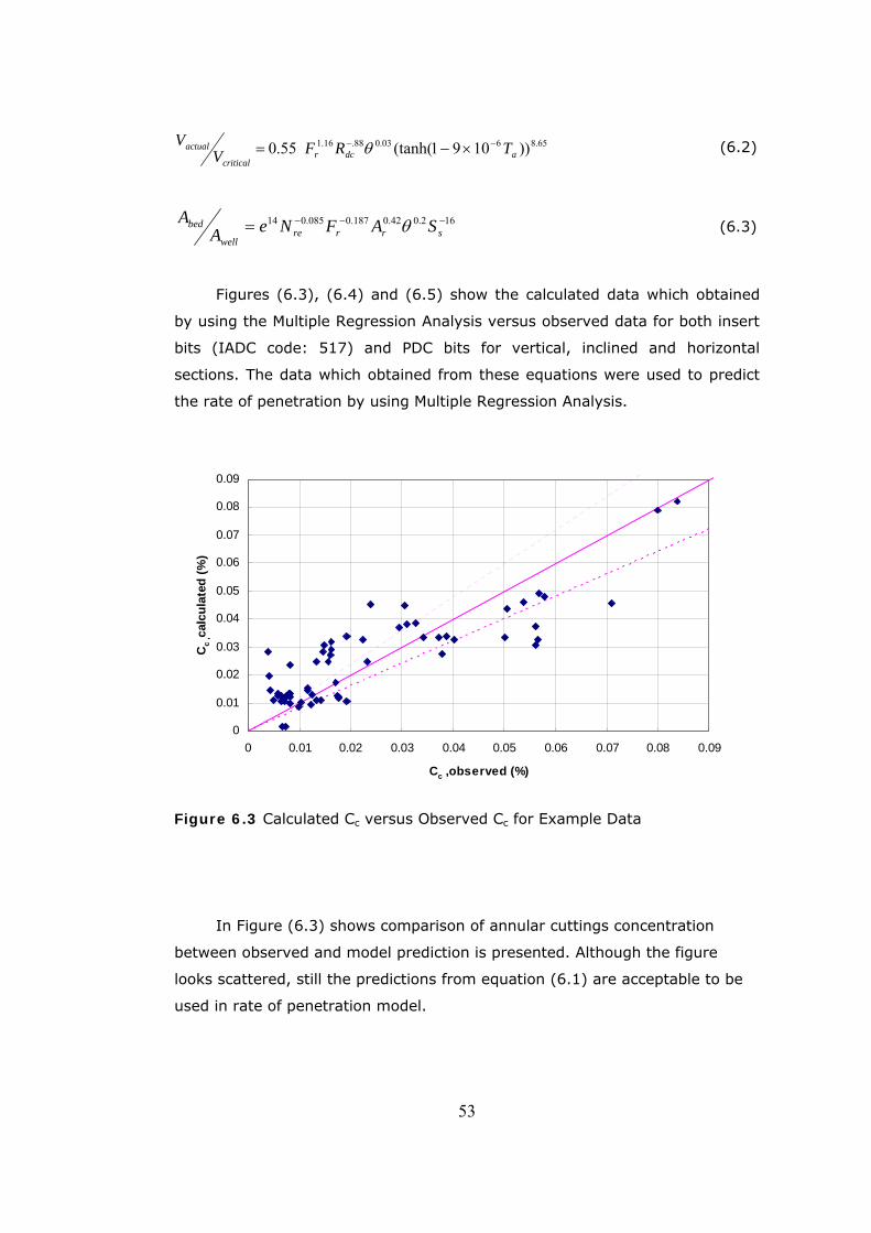
65.8603.088.16.1 ))1091(tanh(55.0 adcr
critical
actual TRFVV −− ×−= θ (6.2)
162.042.0187.0085.014 −−−= srrrewell
bed SAFNeAA θ (6.3)
Figures (6.3), (6.4) and (6.5) show the calculated data which obtained
by using the Multiple Regression Analysis versus observed data for both insert
bits (IADC code: 517) and PDC bits for vertical, inclined and horizontal
sections. The data which obtained from these equations were used to predict
the rate of penetration by using Multiple Regression Analysis.
0
0.01
0.02
0.03
0.04
0.05
0.06
0.07
0.08
0.09
0 0.01 0.02 0.03 0.04 0.05 0.06 0.07 0.08 0.09
Cc ,observed (%)
Cc
,cal
cula
ted
(%)
Figure 6.3 Calculated Cc versus Observed Cc for Example Data
In Figure (6.3) shows comparison of annular cuttings concentration
between observed and model prediction is presented. Although the figure
looks scattered, still the predictions from equation (6.1) are acceptable to be
used in rate of penetration model.
53
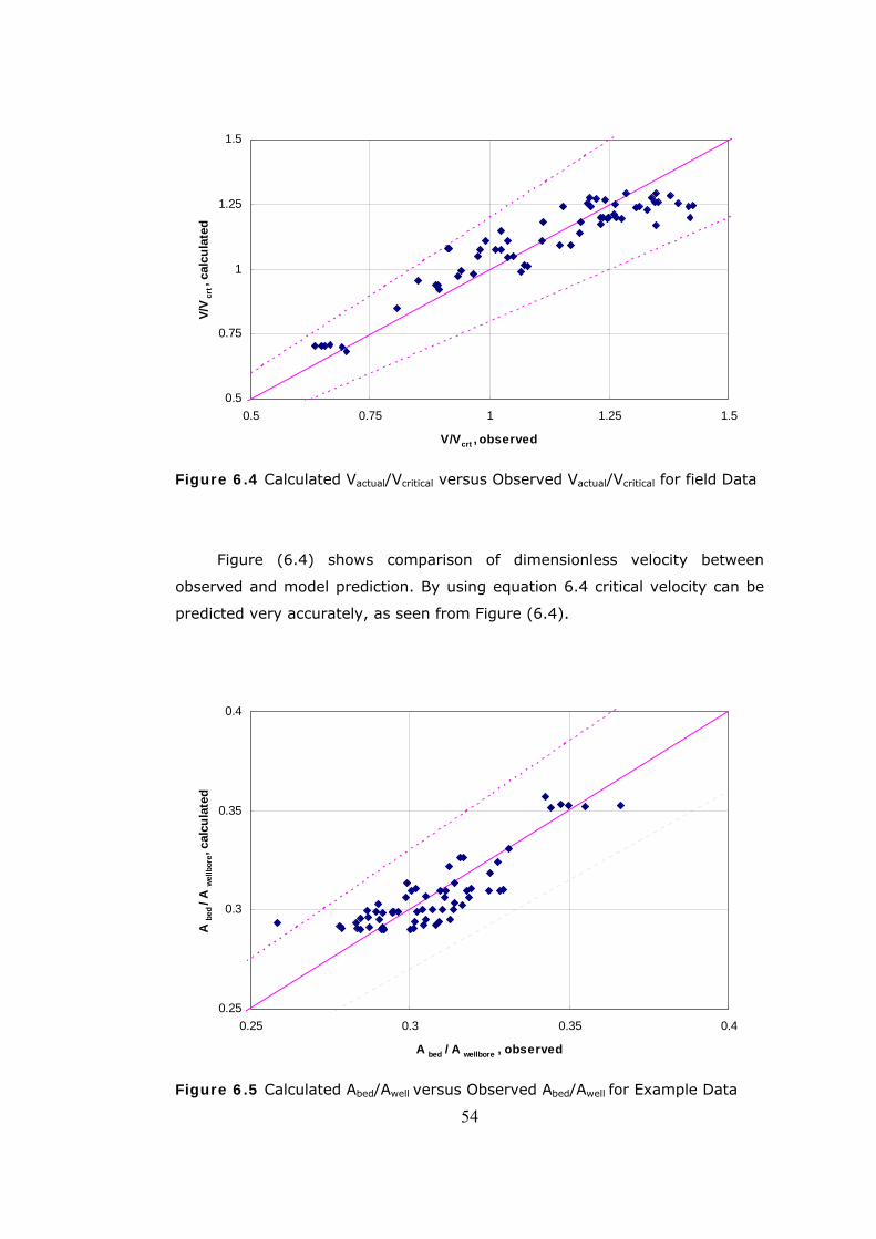
0.5
0.75
1
1.25
1.5
0.5 0.75 1 1.25 1.5
V/Vcrt , observed
V/V
crt ,
calc
ulat
ed
Figure 6.4 Calculated Vactual/Vcritical versus Observed Vactual/Vcritical for field Data
Figure (6.4) shows comparison of dimensionless velocity between
observed and model prediction. By using equation 6.4 critical velocity can be
predicted very accurately, as seen from Figure (6.4).
54
0.25
0.3
0.35
0.4
0.25 0.3 0.35 0.4
A bed / A wellbore , observed
A be
d / A
wel
lbor
e, ca
lcul
ated
Figure 6.5 Calculated Abed/Awell versus Observed Abed/Awell for Example Data
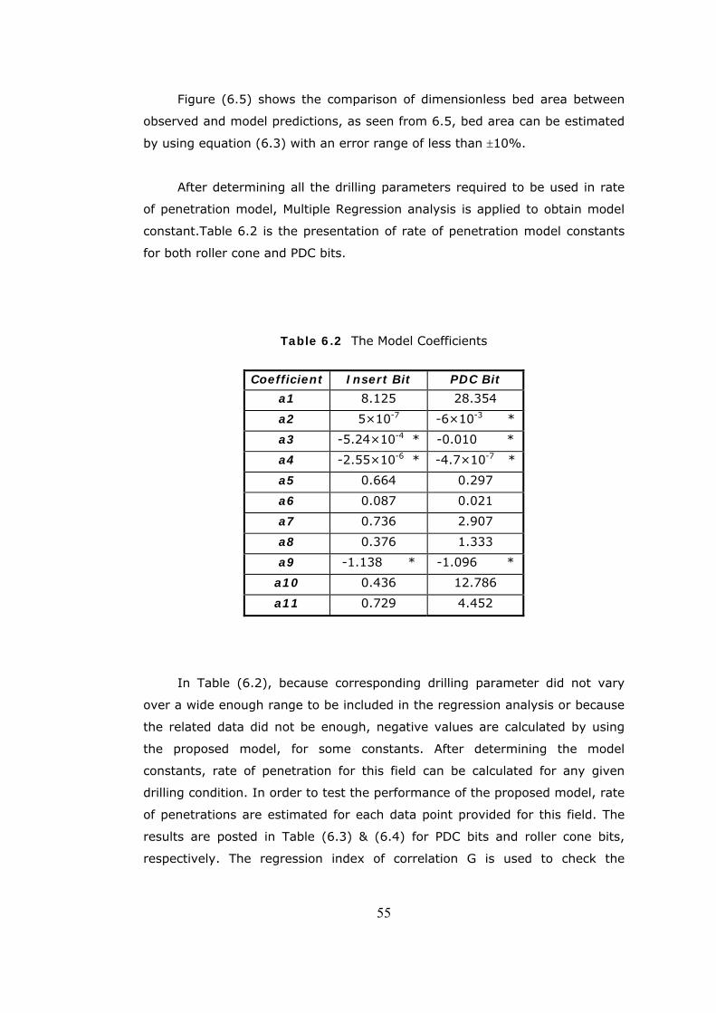
55
Figure (6.5) shows the comparison of dimensionless bed area between
observed and model predictions, as seen from 6.5, bed area can be estimated
by using equation (6.3) with an error range of less than ±10%.
After determining all the drilling parameters required to be used in rate
of penetration model, Multiple Regression analysis is applied to obtain model
constant.Table 6.2 is the presentation of rate of penetration model constants
for both roller cone and PDC bits.
Table 6.2 The Model Coefficients
Coefficient Insert Bit PDC Bit
a1 8.125 28.354
a2 5×10⁻⁷ -6×10⁻³ *
a3 -5.24×10⁻⁴ * -0.010 *
a4 -2.55×10⁻⁶ * -4.7×10⁻⁷ *
a5 0.664 0.297
a6 0.087 0.021
a7 0.736 2.907
a8 0.376 1.333
a9 -1.138 * -1.096 *
a10 0.436 12.786
a11 0.729 4.452
In Table (6.2), because corresponding drilling parameter did not vary
over a wide enough range to be included in the regression analysis or because
the related data did not be enough, negative values are calculated by using
the proposed model, for some constants. After determining the model
constants, rate of penetration for this field can be calculated for any given
drilling condition. In order to test the performance of the proposed model, rate
of penetrations are estimated for each data point provided for this field. The
results are posted in Table (6.3) & (6.4) for PDC bits and roller cone bits,
respectively. The regression index of correlation G is used to check the
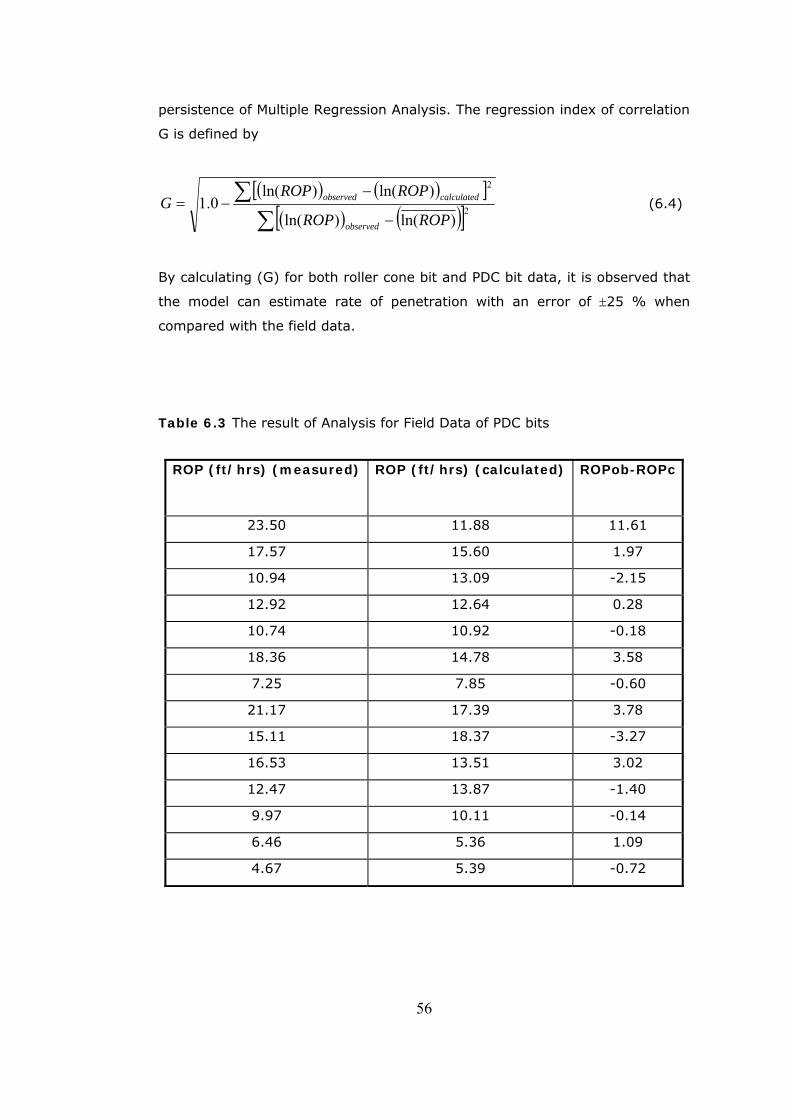
persistence of Multiple Regression Analysis. The regression index of correlation
G is defined by
( ) ( )[ ]( ) ( )[ ]∑
∑−
−−= 2
2
)ln()ln(
)ln()ln(0.1
ROPROP
ROPROPG
observed
calculatedobserved (6.4)
By calculating (G) for both roller cone bit and PDC bit data, it is observed that
the model can estimate rate of penetration with an error of ±25 % when
compared with the field data.
Table 6.3 The result of Analysis for Field Data of PDC bits
ROP (ft/hrs) (measured) ROP (ft/hrs) (calculated) ROPob-ROPc
23.50 11.88 11.61
17.57 15.60 1.97
10.94 13.09 -2.15
12.92 12.64 0.28
10.74 10.92 -0.18
18.36 14.78 3.58
7.25 7.85 -0.60
21.17 17.39 3.78
15.11 18.37 -3.27
16.53 13.51 3.02
12.47 13.87 -1.40
9.97 10.11 -0.14
6.46 5.36 1.09
4.67 5.39 -0.72
56
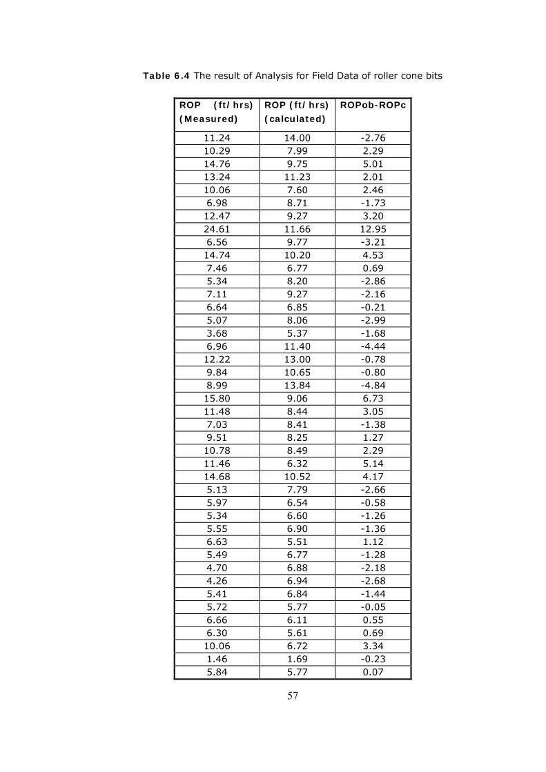
57
Table 6.4 The result of Analysis for Field Data of roller cone bits
ROP (ft/hrs) (Measured)
ROP (ft/hrs) (calculated)
ROPob-ROPc
11.24 14.00 -2.76 10.29 7.99 2.29 14.76 9.75 5.01 13.24 11.23 2.01 10.06 7.60 2.46 6.98 8.71 -1.73 12.47 9.27 3.20 24.61 11.66 12.95 6.56 9.77 -3.21 14.74 10.20 4.53 7.46 6.77 0.69 5.34 8.20 -2.86 7.11 9.27 -2.16 6.64 6.85 -0.21 5.07 8.06 -2.99 3.68 5.37 -1.68 6.96 11.40 -4.44 12.22 13.00 -0.78 9.84 10.65 -0.80 8.99 13.84 -4.84 15.80 9.06 6.73 11.48 8.44 3.05 7.03 8.41 -1.38 9.51 8.25 1.27 10.78 8.49 2.29 11.46 6.32 5.14 14.68 10.52 4.17 5.13 7.79 -2.66 5.97 6.54 -0.58 5.34 6.60 -1.26 5.55 6.90 -1.36 6.63 5.51 1.12 5.49 6.77 -1.28 4.70 6.88 -2.18 4.26 6.94 -2.68 5.41 6.84 -1.44 5.72 5.77 -0.05 6.66 6.11 0.55 6.30 5.61 0.69 10.06 6.72 3.34 1.46 1.69 -0.23 5.84 5.77 0.07
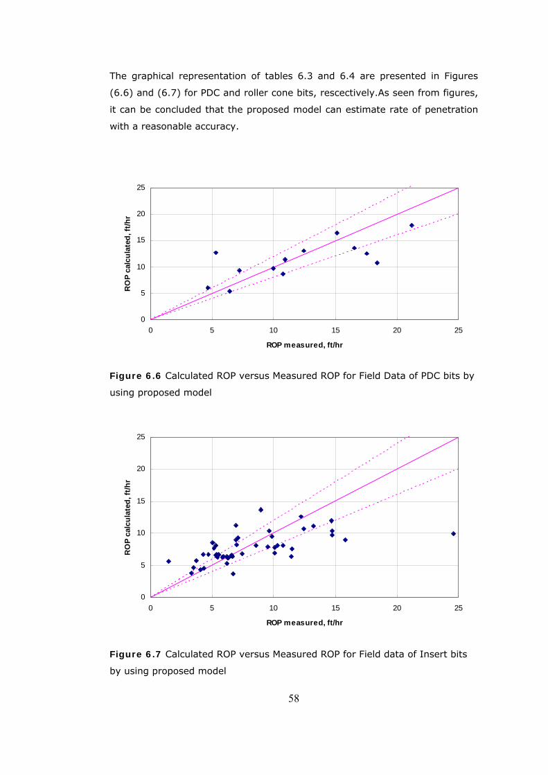
The graphical representation of tables 6.3 and 6.4 are presented in Figures
(6.6) and (6.7) for PDC and roller cone bits, rescectively.As seen from figures,
it can be concluded that the proposed model can estimate rate of penetration
with a reasonable accuracy.
0
5
10
15
20
25
0 5 10 15 20 25
ROP measured, ft/hr
RO
P ca
lcul
ated
, ft/h
r
Figure 6.6 Calculated ROP versus Measured ROP for Field Data of PDC bits by
using proposed model
0
5
10
15
20
25
0 5 10 15 20 25
ROP measured, ft/hr
RO
P ca
lcul
ated
, ft/h
r
Figure 6.7 Calculated ROP versus Measured ROP for Field data of Insert bits
by using proposed model
58
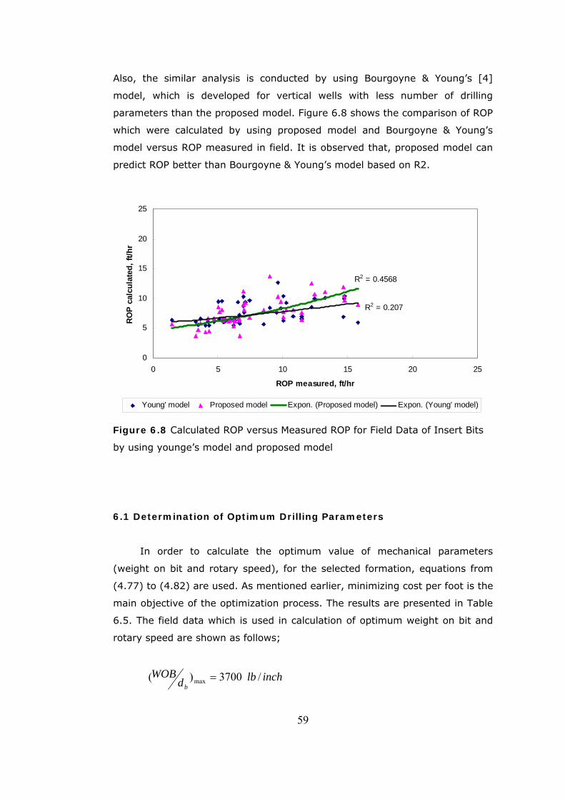
Also, the similar analysis is conducted by using Bourgoyne & Young’s [4]
model, which is developed for vertical wells with less number of drilling
parameters than the proposed model. Figure 6.8 shows the comparison of ROP
which were calculated by using proposed model and Bourgoyne & Young’s
model versus ROP measured in field. It is observed that, proposed model can
predict ROP better than Bourgoyne & Young’s model based on R2.
R2 = 0.4568
R2 = 0.207
0
5
10
15
20
25
0 5 10 15 20 25
ROP measured, ft/hr
RO
P c
alcu
late
d, ft
/hr
Young' model Proposed model Expon. (Proposed model) Expon. (Young' model)
Figure 6.8 Calculated ROP versus Measured ROP for Field Data of Insert Bits
by using younge’s model and proposed model
6.1 Determination of Optimum Drilling Parameters
In order to calculate the optimum value of mechanical parameters
(weight on bit and rotary speed), for the selected formation, equations from
(4.77) to (4.82) are used. As mentioned earlier, minimizing cost per foot is the
main objective of the optimization process. The results are presented in Table
6.5. The field data which is used in calculation of optimum weight on bit and
rotary speed are shown as follows;
inchlbdWOB
b/3700)( max =
59
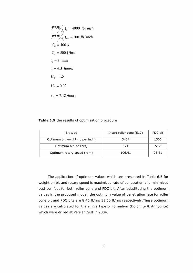
inchlbdWOB
cb
/4000)( =
inchlbdWOB
cirb
/100)( =
400=bC $
500=rC $/hrs
min3=ct
hourstt 5.6=
5.11 =H
02.03 =H
18.7=Hτ Hours
Table 6.5 the results of optimization procedure
Bit type Insert roller cone (517) PDC bit
Optimum bit weight (lb per inch) 3404 1306
Optimum bit life (hrs) 121 517
Optimum rotary speed (rpm) 106.41 93.61
The application of optimum values which are presented in Table 6.5 for
weight on bit and rotary speed is maximized rate of penetration and minimized
cost per foot for both roller cone and PDC bit. After substituting the optimum
values in the proposed model, the optimum value of penetration rate for roller
cone bit and PDC bits are 8.46 ft/hrs 11.60 ft/hrs respectively.These optimum
values are calculated for the single type of formation (Dolomite & Anhydrite)
which were drilled at Persian Gulf in 2004.
60
CHAPTER VII
CONCLUSIONS AND RECOMMENDATIONS
A comprehensive model was developed and successfully used to obtain a
realistic solution to determine the penetration rate for both insert bits (IADC
code: 517 & 523) and PDC bits for inclined and horizontal wells. The model
provides an efficient tool for determining the combined effect of several
variables on the rate of penetration within realistic technological constraints.
At the present time, this approach has been tested only in the Persian Gulf
area and the acceptable results have been obtained. The following conclusions
resulted from this evaluation.
1. Proposed model can estimate rate of penetration as a function of many
drilling variables such as weight on bit, rotary speed, flow rate, nozzle
diameters, drilling fluid density and viscosity, bed height and cuttings
concentration in the annulus with a reasonable accuracy.
2. By using modern well monitoring equipment, the Multiple Regression
Analysis procedure can be applied to determine the regression
coefficients present in the rate of penetration equation.
3. To increase the accuracy of model, it is necessary to use data from
more than a single well. Also, these data should be from a single
formation.
4. By using the mentioned Tooth Wear Model, the calculation of friction
tooth dullness (h) is possible for both tungsten carbide insert bits
(IADC code: 517 & 523) and PDC bits.
5. Because of the structure, geometry and the number and size of their
nozzles of PDC bits, the pump-off force play an effective roll on the
weight on bit.
6. By using the Dimensionless Analysis, the annular cuttings
concentration, Cc, dimensionless equilibrium bed area, Abed/Awell, and
62
dimensionless velocity, Vactual/Vcritical can be predicted with an acceptable
accuracy.
The practical utilization of the model was illustrated by the use of field
data which obtained from several horizontal and inclined wells in the Persian
Gulf area. Analysis has shown that the simulator enhanced the evaluation of
field data and the selection of optimum drilling parameters for a new well to be
drilled in the field of interest. Results have also confined that the use of an
optimization technique as suggested in this study can reduce drilling costs
significantly.
Furthermore, inclusion of cuttings transport parameters in the drilling
optimization of horizontal wells reduces the risk of problems such as abnormal
torque and drag, lost circulation, difficulties in running casing, poor cement
jobs, the necessity of redrilling, and sticking of the drill string.
63
REFERENCES
1. Bardley, W.B. Et Al.: “Task Force Approach to Reducing Stuck Pipe Costs”,
SPE 21999, presented at Amsterdam, 11-14, March 1991.
2. Barragan, R.V., Santos, O.L.A. and Maidla, E.E.: “Optimization of Multiple
Bit Runs”, SPE 37644, 1997 SPE/IADC Drilling Conference, Amsterdam,
The Netherlands, March 1997.
3. Becker, T.E., J.J. Azar, And S.S. Okrajni: “Correlations of Mud Rheology
Properties with Cuttings Transport Performance in Directional Drilling”,
SPE Drilling Engineering, March 1991, pp.16-24
4. Bonet, L., Cunha, J.C.S. and Prado, M.G.: "Drilling Optimization: A New
Approach to Optimize Drilling Parameters and Improve Drilling
Efficiency", Drilling Technology, ASME, 1995.
5. Bourgoyne, A.T., Jr. and Young, F.S., Jr.: "A Multiple Regression Approach
to Optimal Drilling and Abnormal Pressure Detectiony', SPE 4238, SPE-
AIME Sixth Conference on Drilling and Rock Mechanics, Austin, TX,
January 1973.
6. Bourgoyne, A.T., MiIlheim, K.K., Chenevert, M.E. and Young, F.S.:
"Applied Drilling Engineering", SPE Textbook Series, Vol. 2, Richardson, TX, 1986.
7. Brett,F.J. and Millheim,K.K.:” The Drilling Performance Curve: A Yardstick
for Judging Drilling Performance”, 61st Annual Technical Conference
and Exhibition of the Society of Petroleum Engineers,New Orfeans, LA,
October 5-8, 1986.
8. Brown, N.P., P.A.Bern And A.Weaver.: “Cleaning Deviated Holes: New
Experimental and Theoretical Studies”, SPE/IADC 18636 presented at
the 1989 SPE/IADC Drilling Conference, New Orleans, Louisiana,
(February 28-March 3,1989) 171.
64
9. Cho, H.,Subhash, N.Shah And S.O.Osisanya : “A Three-Segment Hydraulic
Model for Cuttings Transport in Horizontal and Deviated Wells”, SPE
65488, presented at 2000 SPE/ Petroleum Society of CIM International
Conference on Horizontal Well Technology, Calgary, Alberta, Canada,
November 6-8, 2000
10. Duklet,P. C. and Bates, T. R.: “AEmperical Correlation to predict Diamond
Bit Drilling Raets”, SPE 9324, 55th Annular Technical Conference and
Exhibition of SPE, Dallas-Texas, September 21-24, 1980.
11. Fear,M.J.:”How to Improve Rate of Penetration in Field Operations”,SPE
55050, IADC/SPE Drilling Conference , New Orleance , USA, March12-
15, 1999.
12. Fullerton, H.B. Jr.,:”Constant Energy Drilling System for Well
Programming”, Compliments of Smith Tool, August,1973.
13. Galle, E.M. and Woods, H.B.: "Best Constant Weight and Rotary Speed for
Rotary Rock Bits", API Drilling and Production Practice, 1963.
14. Galle, E.M. and Woods, H.B.: "Variable Weight and Rotary Speed for
Lowest Drilling Cost", paper presented at 20th Annual Meeting of
AAODC, New Orleans,LA, September 25-27, 1960.
15. Gavignet, A.A. And I.J. Sobey: “Model Aids Cuttings Transport
Predictions”, Jour. of Pet. Tech., Sep. 1989, pp. 916-22
16. Guo,X.Z.:”A Preliminary Investigation on the Objective Function of
Penetration Cost Applied to Optimized Drilling”,International Meeting on
Petroleum Engineering, Beijing,China,March 17-20,1988.
17. Hoover,E.R. and Middleton, J.N.:” Laboratory Evaluation of PDC Drill Bits
Under High-Speed and High-Wear Conditions”,JOURNAL OF PETROLEUM
TECHNOLOGY,p2316-2321, DECEMBER,1981.
18. Hussain Rabia:” Specific Energy as a Criterion for Bit selection”, JOURNAL
OF PETROLEUM TECHNOLOGY,p 1225-1229, JULY,1985.
65
19. Kamp, A.M. And M. Rivero: “Layer Modeling for Cuttings Transport in
Highly Inclined Wellbores”, SPE 53942, Proc. of 1999 SPE Latin
American and Carribean Petroleum Engineering Conference, Caracas,
Venezulea, April 21-23/1999.
20. Kendall, H.A. and Goins, W.C.: 'Design and Operation of Jet-Bit Programs
for Maximum Hydraulic Horsepower, Impact Force and Jet Velocity",
Petroleum Transactions, AIME, Vol. 219, 1960.
21. Kjosnes I., Loklingholm G., Saasen A., Syrstad S.O., Agle A., And Solvang
K.A.; “Successful Water Based Drilling Fluid Design for Optimizing Hole
Cleaning and Hole Stability”, SPE 85330, Presented at SPE/IADC Middle
East Drilling Techology Conference and Exhibition, abu Dhabi, UAE, 20-
22 October, 2003
22. Larsen, T.I., A.A. Pilehvari And J.J. Azar: “Development of a New Cuttings
Transport Model for High-Angle Wellbores Including Horizontal Wells”,
SPE Drilling&Completion, Jun. 1997, pp. 129-35.
23. Langston, J.W.:” A Methtid of Utilizing Existing Information To optimize
Drilling Procedures”Annual Fall Meeting, Denver, Colo, Oct 1965
24. Lummus, J. L.:"Drilling Optimization", JOURNAL OF PETROLEUM
TECHNOLOGY,p1379, NOV 1970.
25. Lummus, J. L.: “Acquisit.im and Analysis of Data for Optimized ” JOURNAL
OF PETROLEUM TECHNOLOGY,p1285-1293, NOV 1971.
26. Lummus, J. L and Azar, J. J: ’’Drilling fluid Optimization—a Practical Field
Approach’’ Penn Well, Tulsa, 1986
27. Malguarnera,S.C.:” The Use of a Drilling Model in Simulation, Optimization,
and Formation Description”, lADC/SPE Drilling Conference, Dallas, TX,
February 10-12, 1986.
66
28. Masuda Y., Q. Doan, M. Oguztoreli, S. Naganawa, T. Yonezawa, A.
Kobayashi, A. Kamp: “Critical Cuttings Transport Velocity in Inclined
Annulus: Experimental Studies and Numerical Simulation”, SPE 65502,
2000 SPE/Petroleum Society of CIM International Conference on
Horizontal Well Technology, Calgary, Alberta, Canada, 6-8 November
2000.
29. Maurer, W.C.: "The 'Perfect-Cleaning' Theory of Rotary Drilling", Journal of
Petroleum Technology, November, 1962.
30. Mechem,O.E. and Fullerton, H.B.Jr.,:”Computers invade the rig floor” Oil
and Gas Journal,p14,1965.
31. Miska, S. and Ziaja, M..B:”Mathematical Model of the Diamond- Bit Drilling
Process and Its Practical Application”, Annual Fall Meeting of the
Society of Petroleum Engineers of AIME, December,1982.
32. Miska,S. and Duan,M.:”Transport of Small Cutting in Extended Reach
Drilling”,International Oil&Gas Conference and Exhibition, Beijing,
China, 5-7 December,2006.
33. Millheim, K.K and Huggins, R.L.: "An Engineering Simulator for Drilling:
Part I", paper presented at the 58" Annual Technical Conference and
Exhibition, San Francisco, CA, October 5-8, 1983.
34. Moore, P.L.: 'Five Factors that Affect Drilling Rate", The Oil and Gas
Journal, October 6, 1958.
35. Nguyen, D. And S.S. Rahman: “A Three-Layer Hydraulic Program for
Effective Cuttings Transport and Hole Cleaning in Highly Deviated and
Horizontal Wells”, SPE Drilling & Completion, Sep. 1998, pp. 182-9.
36. Ozbayoglu, Evren M. Stefan Z. Miska, Troy Reed, Nicholas Takach,
“ Analysis of Bed Height in Horizontal and Highly-Inclined Well bores by
Using Artificial Neuraletworks “ SPE—78939,2002
67
37. Ozbayoglu M.E., Miska Z.S., Reed T., Takach N., “Using Foam in Horizontal
Well Drilling: A Cuttings Transport Approach”, Journal of Petroleum
Science and Engineering, Vol.46, No:4, 267-282, April 2005
38. Parker, EJ., Collins, P.M., Pelli, F. and Brancato, C.D.M.: "Cost Reduction
Through Drilling Optimization", paper presented at the Offshore
39. Pereira J. J:’’ Comprehensive Optimization of Drilling Parameters for
Horizontal Wells’’. Ph. D Thesis.The University of Tulsa,Tulsa. OK.
1999
40. Reed, R-L.: ""A Monte Carlo Approach to Optimal Drillingy', SPE 3513, 46&
Annual Fall Meeting, New Orleans, LA, October 1972.
41. Reza, M.R and Alcocer, C.F.: "A Unique Computer Simulation Model Well
Drilling: Part I - The Reza Drilling Model", SPE 15108, 56" California
Meeting of the Society of Petroleum Engineers, Oakkand, CA, April 2-4,
1986.
42. Robello Samuel, EnerTech-Landmark Graphics, and Stefan Miska:’’
Optimization of Drilling Parameters with the Performance of Positive
Displacement Motor (PDM)’’ SPE—47791.1998
43. Saasen A. And Loklingholm G.; “The Effect of Drilling Fluid Rheological
Properties on Hole Cleaning”, SPE 74558, Presented at IADC/SPE
Drilling Conference, Dallas TX, 26-28 February, 2002.
44. Saasen A., Eriksen N.H., Han Liqun, Labes P. And Marken D., “Is Annular
Friction Loss the Key Parameter?”, Oil Gas European Magazine,
(1)1998, pp.22-24
45. Sanchez, R.A., J.J. Azar, A.A. Bassal, And A.L. Martins: “Effect of Drillpipe
Rotation on Hole Cleaning During Directional-Well Drilling”, SPE Journal,
Jun. 1999, pp. 101-108.
46. Sifferman, T.R. And Becker, T.E.: “Hole Cleaning in Full-Scale Inclined
Wellbores”, SPED, June 1992, p.115-120
68
47. Simmons,E.L.:”A Technique for Accurate Bit Programming and Drilling
Performance Optimization“,lADC/SPE Drilling Conference,Dallas,TX,
Fabruary 10-12,1986.
48. Tanseu,E.:” A Heuristic Approach to Drilling Optimization “,50th Annual
Fall Meeting of the Society of Petroleun Engineers of AIME,Dallas,
Texas, Sept. 28-Oct.1,1975.
49. Tomren, P.H., A.W. Iyoho And J.J. Azar: “An Experimental Study of
Cuttings Transport in Directional Wells”, SPE Drilling Engineering, Feb.
1986, pp. 43-56
50. Warren, T.M.:"Penetration-Rate Performance of Roller-Cone Bits", paper
presented at the 59nd Annual Technical Conference and Exhibition,
Houston, TX, September 16-19, 1984.
51. Wilson, D.C and Bentsen, R.G.:” Optimization Techniques for Minimizing
Drilling Costs”, 47th Annual Fall Meeting of the Society of Petroleum
Engineers of AIME,San Antonio, Tex., Oct. 8-11, 1972.
52. Winters, W.J., Warren, T.M. and Onyia, E.C.: " Roller Bit Model With Rock
Ductility and Cone Offset", paper presented at the 62nd Annual
Technical and Exhibition of the Society of Petroleum Engineers, Dallas,
TX September 27-30, 1987.
53. Wojtanowicz, A.K., and Kuru, E.: “Minimum-Cost Well Drilling Strategy
Using Dynamic Programming”, Joumal of Energy Resources Technology,
Transactions of the ASME, December 1993.
54. Wojtanowicz, A.K., and Kuru, E.:” Dynamic Drilling Strategy for PDC Bits”, SPE/IADC Drilling Conference,New Orleans,LA,March 15-18,1987.
Mediterranean Conference a . Exhibition, Ravenna, Italy, March 15-1 7,
1995.
55. Young, F.S., Jr.: "Computerized Drilling Control", SPE 2241, 43nd Annual
Fall Meeting, Houston, TX, September 1968.

69
56. Yu, M., D. Melcher, N. Takach, S.Z. Miska, R. Ahmed: “A New Approach to
Improve Cuttings Transport in Horizontal and Inclined Wells”, SPE
Paper 90529 presented at the SPE Annual Technical Conference and
Exhibition, Houston, Texas,USA., Sept. 26-29, 2004.
57. Estes, J. C. :’’ selecting the Proper Rotary Rock Bit, ” J. Pet. Tech (Nov.
1971) 1359-1367.
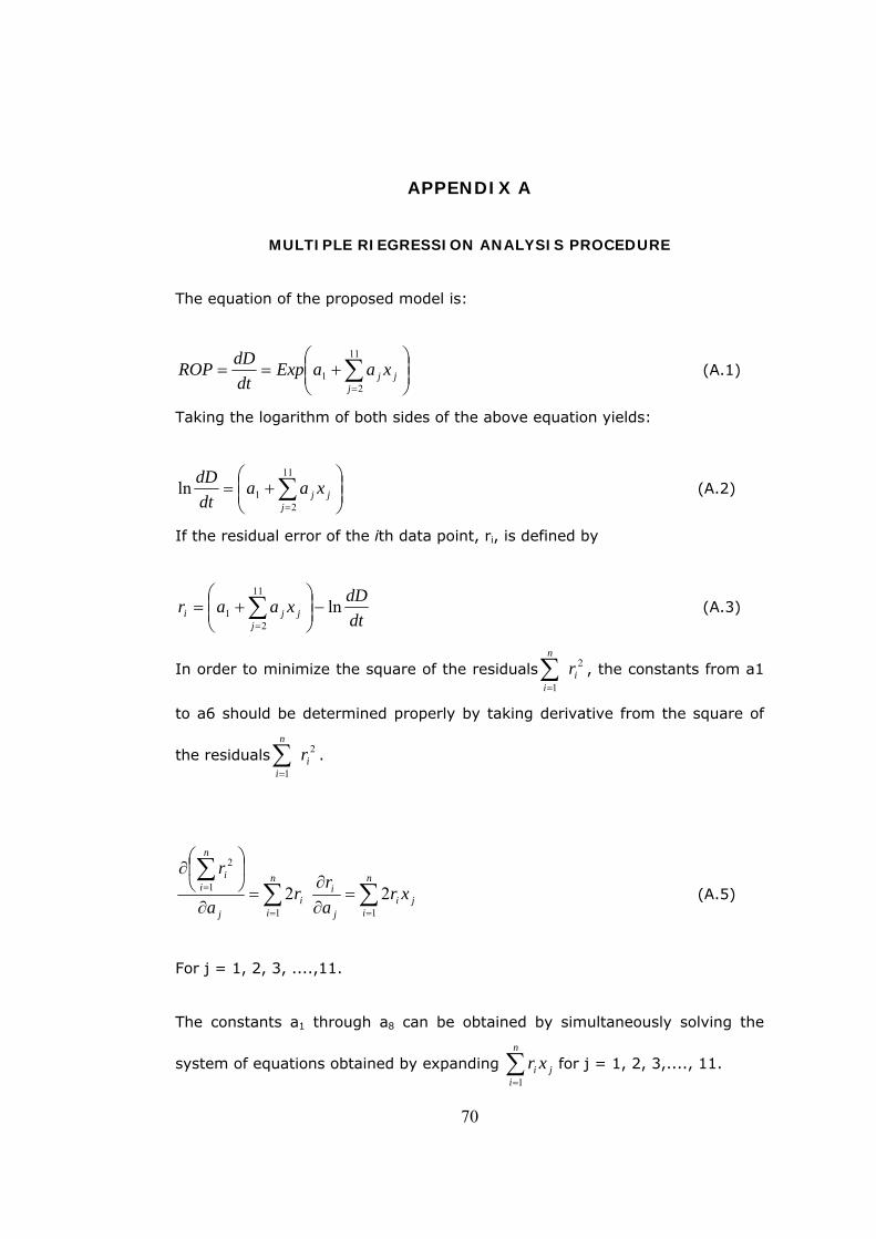
APPENDIX A
MULTIPLE RIEGRESSION ANALYSIS PROCEDURE
The equation of the proposed model is:
⎟⎟⎠
⎞⎜⎜⎝
⎛+== ∑
=
11
21
jjj xaaExp
dtdDROP (A.1)
Taking the logarithm of both sides of the above equation yields:
⎟⎟⎠
⎞⎜⎜⎝
⎛+= ∑
=
11
21ln
jjj xaa
dtdD
(A.2)
If the residual error of the ith data point, ri, is defined by
dtdDxaar
jjji ln
11
21 −⎟⎟
⎠
⎞⎜⎜⎝
⎛+= ∑
=
(A.3)
In order to minimize the square of the residuals , the constants from a1
to a6 should be determined properly by taking derivative from the square of
the residuals .
2
1i
n
i
r∑=
2
1i
n
ir∑
=
∑∑∑
==
= =∂∂
=∂
⎟⎠
⎞⎜⎝
⎛∂
n
iji
j
in
ii
j
n
ii
xrar
ra
r
11
1
2
22 (A.5)
For j = 1, 2, 3, ....,11.
The constants a1 through a8 can be obtained by simultaneously solving the
system of equations obtained by expanding ∑ for j = 1, 2, 3,...., 11. =
n
iji xr
1
70
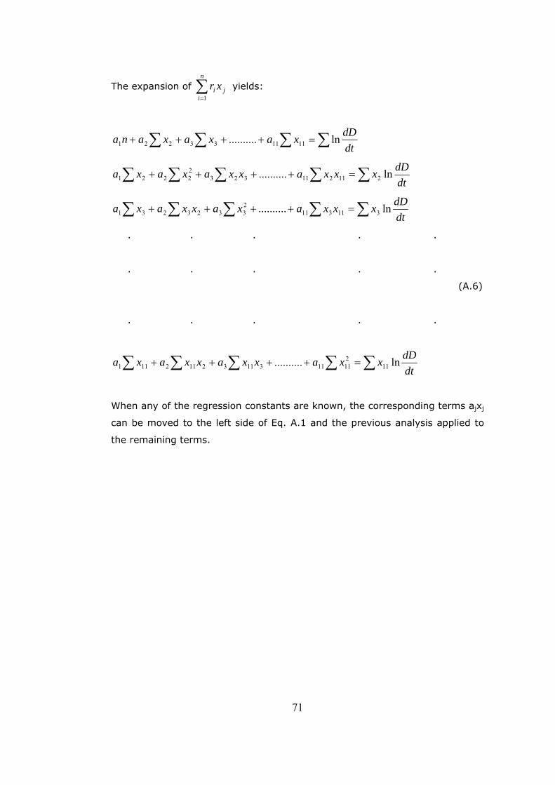
The expansion of yields: ∑=
n
iji xr
1
∑ ∑∑∑ =++++dtdDxaxaxana ln.......... 111133221
∑ ∑∑∑∑ =++++dtdDxxxaxxaxaxa ln.......... 211211323
22221
∑ ∑∑∑∑ =++++dtdDxxxaxaxxaxa ln.......... 311311
23323231
. . . . .
. . . . .
(A.6)
. . . . .
∑ ∑∑∑∑ =++++dtdDxxaxxaxxaxa ln.......... 11
2111131132112111
When any of the regression constants are known, the corresponding terms ajxj
can be moved to the left side of Eq. A.1 and the previous analysis applied to
the remaining terms.
71
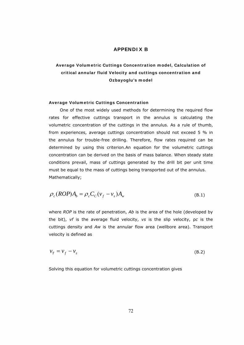
APPENDIX B
Average Volumetric Cuttings Concentration model, Calculation of
critical annular fluid Velocity and cuttings concentration and
Ozbayoglu’s model
Average Volumetric Cuttings Concentration
One of the most widely used methods for determining the required flow
rates for effective cuttings transport in the annulus is calculating the
volumetric concentration of the cuttings in the annulus. As a rule of thumb,
from experiences, average cuttings concentration should not exceed 5 % in
the annulus for trouble-free drilling. Therefore, flow rates required can be
determined by using this criterion.An equation for the volumetric cuttings
concentration can be derived on the basis of mass balance. When steady state
conditions prevail, mass of cuttings generated by the drill bit per unit time
must be equal to the mass of cuttings being transported out of the annulus.
Mathematically;
wsfCcbc AvvCAROP )()( −= ρρ (B.1)
where ROP is the rate of penetration, Ab is the area of the hole (developed by
the bit), vf is the average fluid velocity, vs is the slip velocity, ρc is the
cuttings density and Aw is the annular flow area (wellbore area). Transport
velocity is defined as
sfT vvv −= (B.2)
Solving this equation for volumetric cuttings concentration gives
72
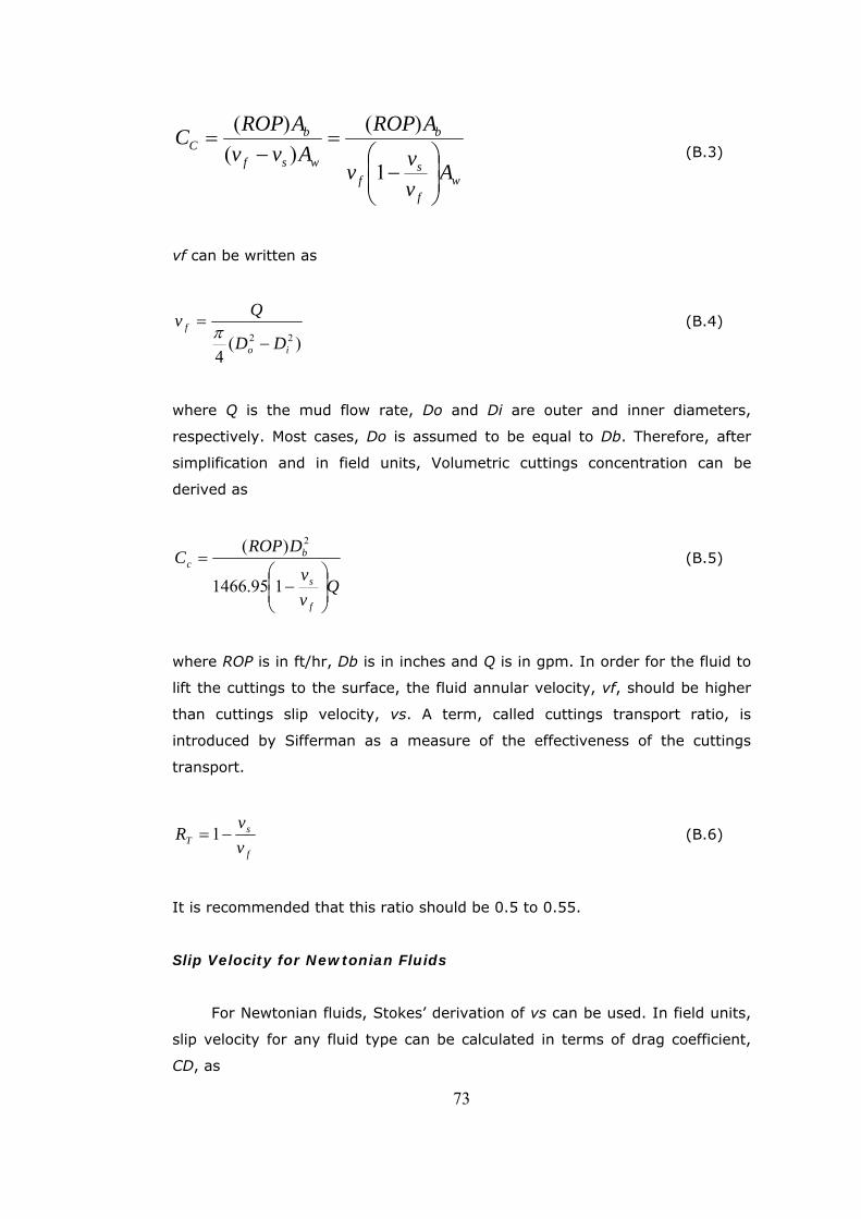
wf
sf
b
wsf
bC
Avvv
AROPAvv
AROPC
⎟⎟⎠
⎞⎜⎜⎝
⎛−
=−
=
1
)()(
)( (B.3)
vf can be written as
)(4
22io
f
DD
Qv−
=π
(B.4)
where Q is the mud flow rate, Do and Di are outer and inner diameters,
respectively. Most cases, Do is assumed to be equal to Db. Therefore, after
simplification and in field units, Volumetric cuttings concentration can be
derived as
Qvv
DROPC
f
s
bc
⎟⎟⎠
⎞⎜⎜⎝
⎛−
=
195.1466
)( 2
(B.5)
where ROP is in ft/hr, Db is in inches and Q is in gpm. In order for the fluid to
lift the cuttings to the surface, the fluid annular velocity, vf, should be higher
than cuttings slip velocity, vs. A term, called cuttings transport ratio, is
introduced by Sifferman as a measure of the effectiveness of the cuttings
transport.
f
sT v
vR −= 1 (B.6)
It is recommended that this ratio should be 0.5 to 0.55.
Slip Velocity for Newtonian Fluids
For Newtonian fluids, Stokes’ derivation of vs can be used. In field units,
slip velocity for any fluid type can be calculated in terms of drag coefficient,
CD, as
73
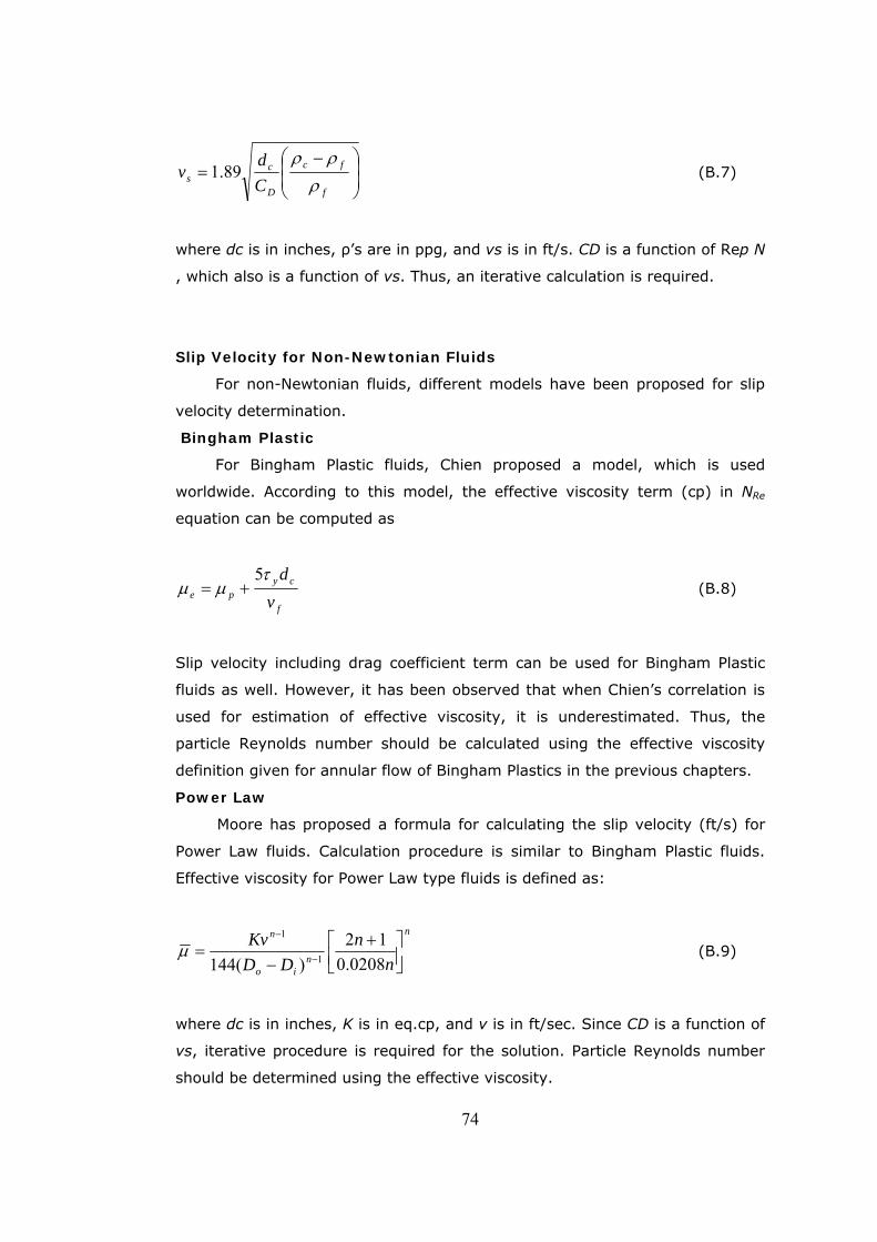
⎟⎟⎠
⎞⎜⎜⎝
⎛ −=
f
fc
D
cs C
dv
ρρρ
89.1 (B.7)
where dc is in inches, ρ’s are in ppg, and vs is in ft/s. CD is a function of Rep N
, which also is a function of vs. Thus, an iterative calculation is required.
Slip Velocity for Non-Newtonian Fluids
For non-Newtonian fluids, different models have been proposed for slip
velocity determination.
Bingham Plastic
For Bingham Plastic fluids, Chien proposed a model, which is used
worldwide. According to this model, the effective viscosity term (cp) in NRe
equation can be computed as
f
cype v
dτμμ
5+= (B.8)
Slip velocity including drag coefficient term can be used for Bingham Plastic
fluids as well. However, it has been observed that when Chien’s correlation is
used for estimation of effective viscosity, it is underestimated. Thus, the
particle Reynolds number should be calculated using the effective viscosity
definition given for annular flow of Bingham Plastics in the previous chapters.
Power Law
Moore has proposed a formula for calculating the slip velocity (ft/s) for
Power Law fluids. Calculation procedure is similar to Bingham Plastic fluids.
Effective viscosity for Power Law type fluids is defined as:
n
nio
n
nn
DDKv
⎥⎦⎤
⎢⎣⎡ +
−= −
−
0208.012
)(144 1
1
μ (B.9)
where dc is in inches, K is in eq.cp, and v is in ft/sec. Since CD is a function of
vs, iterative procedure is required for the solution. Particle Reynolds number
should be determined using the effective viscosity.
74
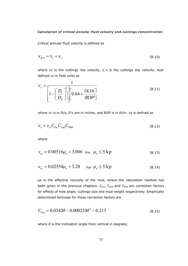
Calculation of critical annular fluid velocity and cuttings concentration
Critical annular fluid velocity is defined as
scfcrt vvv += (B.10)
where vc is the cuttings rise velocity, s v is the cuttings slip velocity. Azar
defined vc in field units as
⎥⎦⎤
⎢⎣⎡ +⎥⎥⎦
⎤
⎢⎢⎣
⎡⎟⎟⎠
⎞⎜⎜⎝
⎛−
=
ROPDD
v
o
i
c16.1864.01
12 (B.11)
where vc is in ft/s, D’s are in inches, and ROP is in ft/hr. vs is defined as
MWsizeinccss CCCvv = (B.12)
where
006.300516.0 += ecsv μ For cpe 53≤μ (B.13)
28.302554.0 += ecsv μ For cpe 53≥μ (B.14)
μe is the effective viscosity of the mud, where the calculation method has
been given in the previous chapters. Cinc, Csize and CMW are correction factors
for effects of hole angle, cuttings size and mud weight respectively. Empirically
determined formulas for these correction factors are
213.0000233.00342.0 2 −−= θθincC (B.15)
where θ is the inclination angle from vertical in degrees;
75
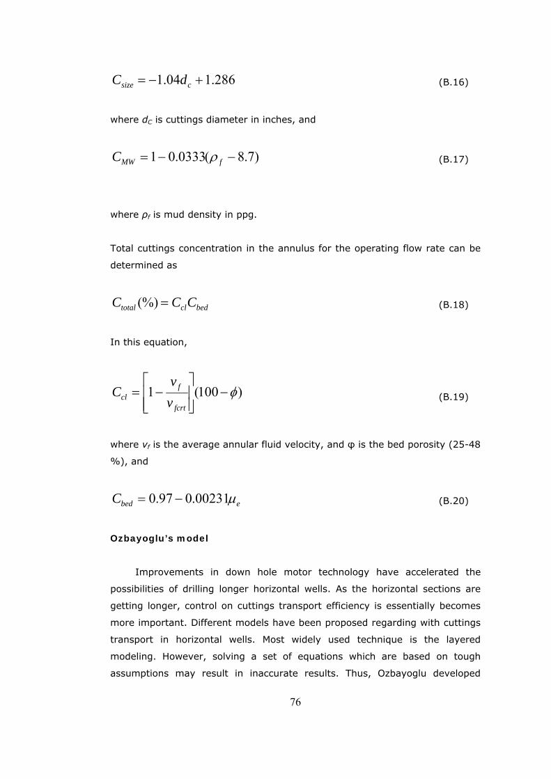
286.104.1 +−= csize dC (B.16)
where dC is cuttings diameter in inches, and
)7.8(0333.01 −−= fMWC ρ (B.17)
where ρf is mud density in ppg.
Total cuttings concentration in the annulus for the operating flow rate can be
determined as
bedcltotal CCC =(%) (B.18)
In this equation,
)100(1 φ−⎥⎥⎦
⎤
⎢⎢⎣
⎡−=
fcrt
fcl v
vC (B.19)
where vf is the average annular fluid velocity, and φ is the bed porosity (25-48
%), and
ebedC μ00231.097.0 −= (B.20)
Ozbayoglu’s model
Improvements in down hole motor technology have accelerated the
possibilities of drilling longer horizontal wells. As the horizontal sections are
getting longer, control on cuttings transport efficiency is essentially becomes
more important. Different models have been proposed regarding with cuttings
transport in horizontal wells. Most widely used technique is the layered
modeling. However, solving a set of equations which are based on tough
assumptions may result in inaccurate results. Thus, Ozbayoglu developed
76
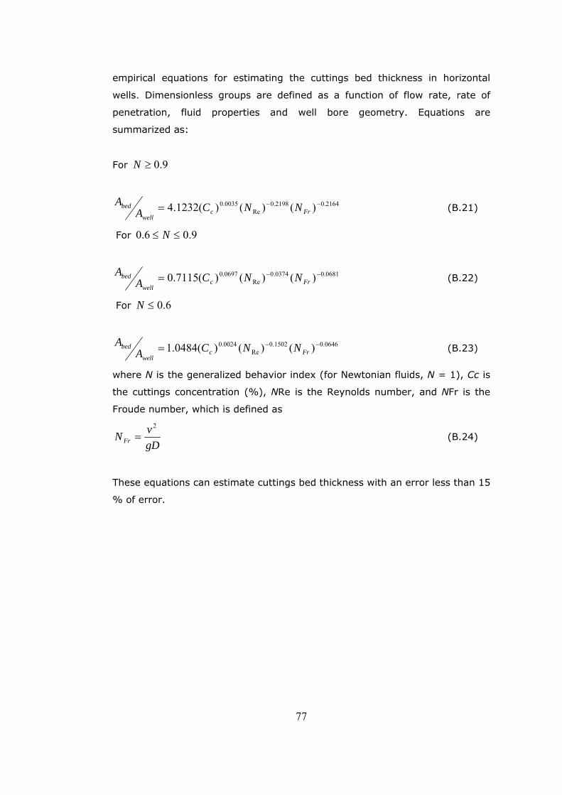
empirical equations for estimating the cuttings bed thickness in horizontal
wells. Dimensionless groups are defined as a function of flow rate, rate of
penetration, fluid properties and well bore geometry. Equations are
summarized as:
For 9.0≥N
2164.02198.0Re
0035.0 )()()(1232.4 −−= Frcwell
bed NNCAA (B.21)
For 9.06.0 ≤≤ N
0681.00374.0Re
0697.0 )()()(7115.0 −−= Frcwell
bed NNCAA (B.22)
For 6.0≤N
0646.01502.0Re
0024.0 )()()(0484.1 −−= Frcwell
bed NNCAA (B.23)
where N is the generalized behavior index (for Newtonian fluids, N = 1), Cc is
the cuttings concentration (%), NRe is the Reynolds number, and NFr is the
Froude number, which is defined as
gDvN Fr
2
= (B.24)
These equations can estimate cuttings bed thickness with an error less than 15
% of error.
77
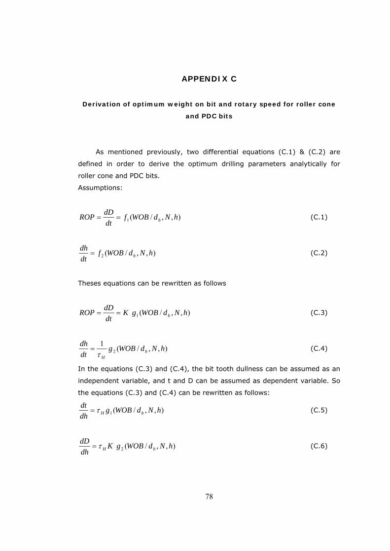
APPENDIX C
Derivation of optimum weight on bit and rotary speed for roller cone
and PDC bits
As mentioned previously, two differential equations (C.1) & (C.2) are
defined in order to derive the optimum drilling parameters analytically for
roller cone and PDC bits.
Assumptions:
),,/(1 hNdWOBfdtdDROP b== (C.1)
),,/(2 hNdWOBfdtdh
b= (C.2)
Theses equations can be rewritten as follows
),,/(1 hNdWOBgKdtdDROP b== (C.3)
),,/(12 hNdWOBg
dtdh
bHτ
= (C.4)
In the equations (C.3) and (C.4), the bit tooth dullness can be assumed as an
independent variable, and t and D can be assumed as dependent variable. So
the equations (C.3) and (C.4) can be rewritten as follows:
),,/(1 hNdWOBgdhdt
bHτ= (C.5)
),,/(2 hNdWOBgKdhdD
bHτ= (C.6)
78
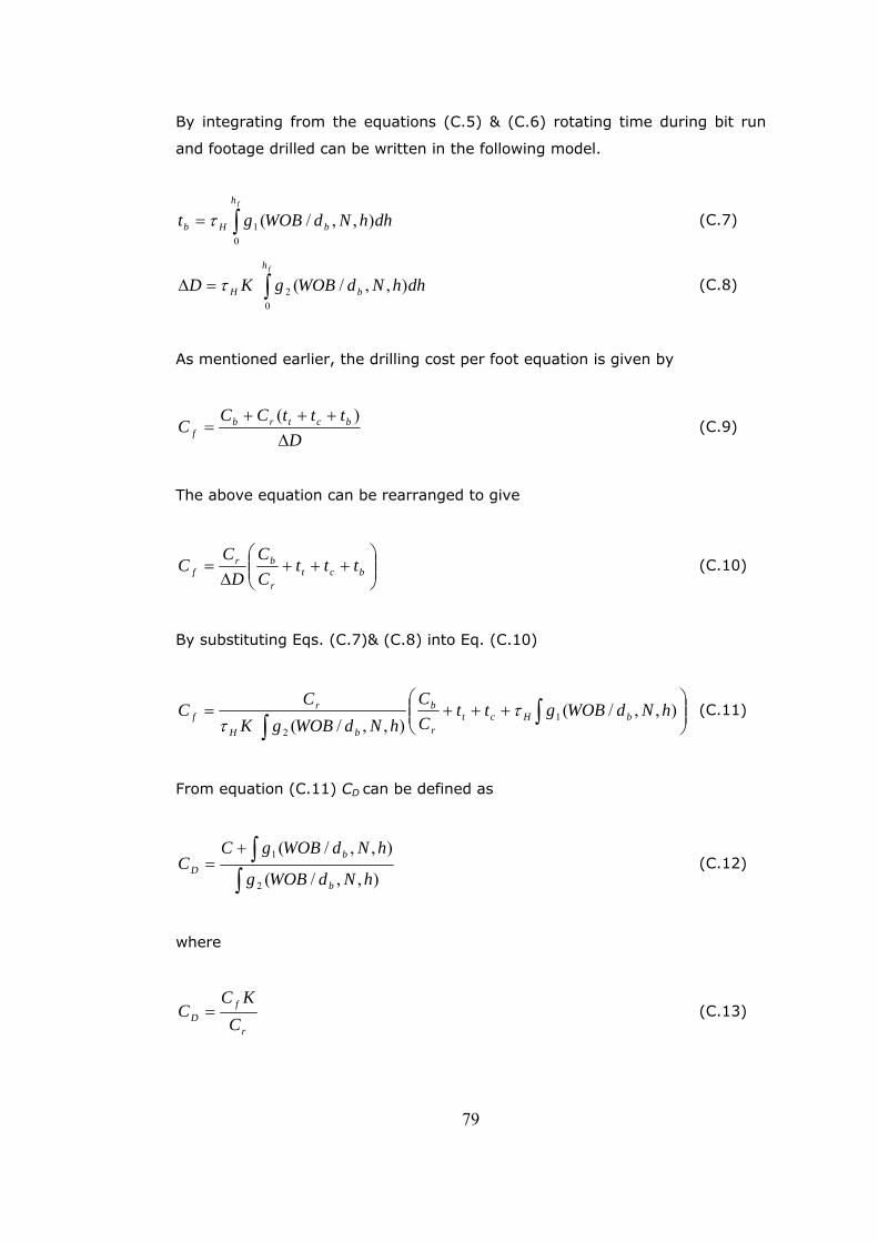
By integrating from the equations (C.5) & (C.6) rotating time during bit run
and footage drilled can be written in the following model.
dhhNdWOBgt b
h
Hb
f
),,/(0
1∫= τ (C.7)
dhhNdWOBgKD b
h
H
f
),,/(0
2∫=Δ τ (C.8)
As mentioned earlier, the drilling cost per foot equation is given by
DtttCC
C bctrbf Δ
+++=
)( (C.9)
The above equation can be rearranged to give
⎟⎟⎠
⎞⎜⎜⎝
⎛+++
Δ= bct
r
brf ttt
CC
DC
C (C.10)
By substituting Eqs. (C.7)& (C.8) into Eq. (C.10)
⎟⎟⎠
⎞⎜⎜⎝
⎛+++= ∫∫
),,/(),,/( 1
2
hNdWOBgttCC
hNdWOBgKC
C bHctr
b
bH
rf τ
τ (C.11)
From equation (C.11) CD can be defined as
∫∫+=
),,/(
),,/(
2
1
hNdWOBg
hNdWOBgCC
b
bD (C.12)
where
r
fD C
KCC = (C.13)
79
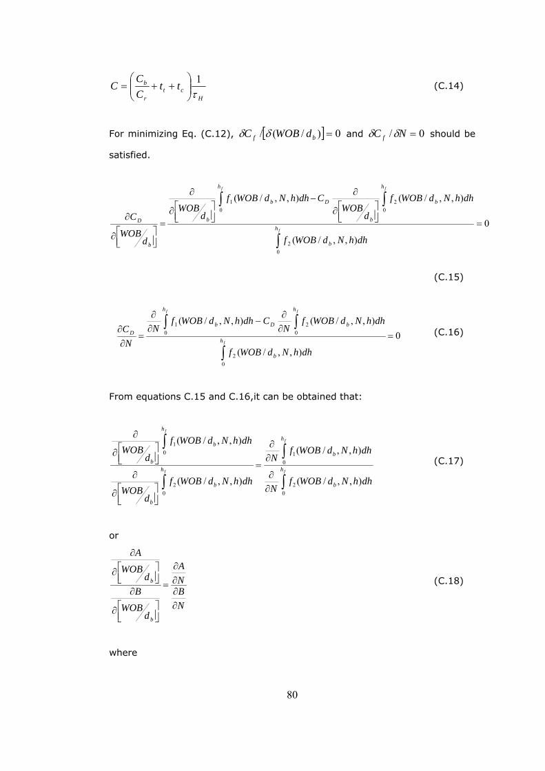
Hct
r
b ttCC
Cτ1
⎟⎟⎠
⎞⎜⎜⎝
⎛++= (C.14)
For minimizing Eq. (C.12), [ ] 0)/(/ =bf dWOBC δδ and 0/ =NC f δδ should be
satisfied.
0
),,/(
),,/(),,/(
02
0 021
=⎥⎦⎤
⎢⎣⎡∂
∂−
⎥⎦⎤
⎢⎣⎡∂
∂
=
⎥⎦⎤
⎢⎣⎡∂
∂
∫
∫ ∫
f
f f
h
b
h h
b
b
Db
b
b
D
dhhNdWOBf
dhhNdWOBf
dWOB
CdhhNdWOBf
dWOB
dWOB
C
(C.15)
0
),,/(
),,/(),,/(
02
0 021
=∂∂
−∂∂
=∂∂
∫
∫ ∫f
f f
h
b
h h
bDbD
dhhNdWOBf
dhhNdWOBfN
CdhhNdWOBfN
NC (C.16)
From equations C.15 and C.16,it can be obtained that:
∫
∫
∫
∫
∂∂
∂∂
=
⎥⎦⎤
⎢⎣⎡∂
∂
⎥⎦⎤
⎢⎣⎡∂
∂
f
f
f
f
h
b
h
b
h
b
b
h
b
b
dhhNdWOBfN
dhhNdWOBfN
dhhNdWOBf
dWOB
dhhNdWOBf
dWOB
02
01
02
01
),,/(
),,/(
),,/(
),,/(
(C.17)
or
NBNA
dWOB
Bd
WOB
A
b
b
∂∂∂∂
=
⎥⎦⎤
⎢⎣⎡∂
∂⎥⎦⎤
⎢⎣⎡∂
∂
(C.18)
where
80
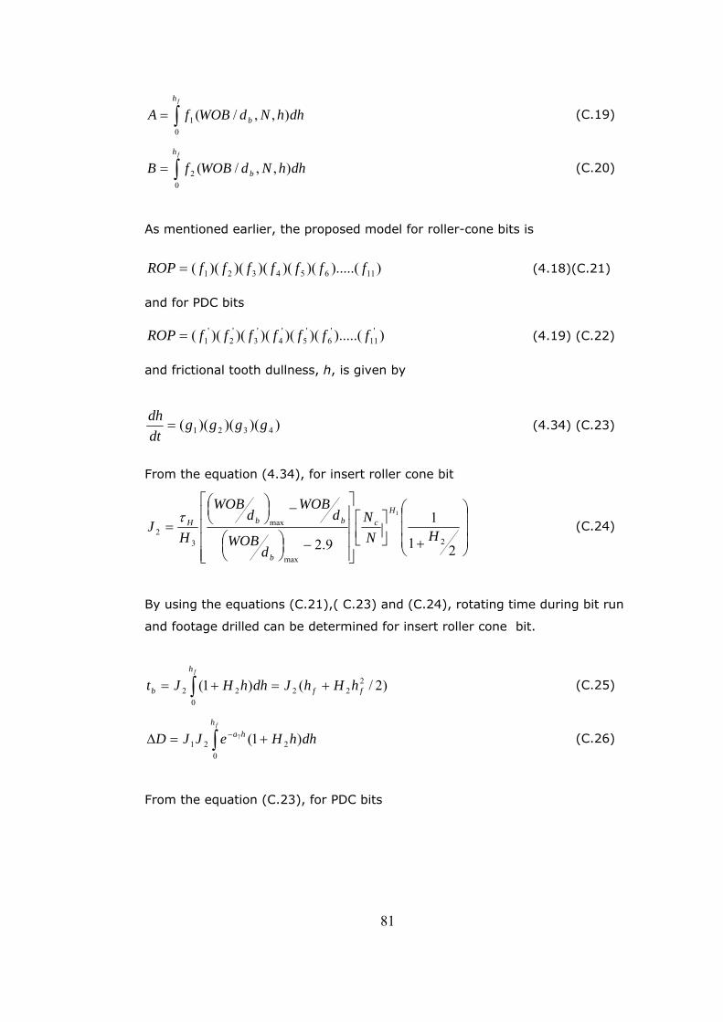
dhhNdWOBfA b
h f
),,/(0
1∫= (C.19)
dhhNdWOBfB b
h f
),,/(0
2∫= (C.20)
As mentioned earlier, the proposed model for roller-cone bits is
)).....()()()()()(( 11654321 fffffffROP = (4.18)(C.21)
and for PDC bits
)).....()()()()()(( '11
'6
'5
'4
'3
'2
'1 fffffffROP = (4.19) (C.22)
and frictional tooth dullness, h, is given by
))()()(( 4321 ggggdtdh
= (4.34) (C.23)
From the equation (4.34), for insert roller cone bit
⎟⎟⎟
⎠
⎞
⎜⎜⎜
⎝
⎛
+⎥⎦⎤
⎢⎣⎡
⎥⎥⎥⎥
⎦
⎤
⎢⎢⎢⎢
⎣
⎡
−⎟⎠⎞⎜
⎝⎛
−⎟⎠⎞⎜
⎝⎛
=
21
1
9.2 2
max
max
32
1
HNN
dWOB
dWOB
dWOB
HJ
Hc
b
bbHτ (C.24)
By using the equations (C.21),( C.23) and (C.24), rotating time during bit run
and footage drilled can be determined for insert roller cone bit.
)2/()1( 222
022 ff
h
b hHhJdhhHJtf
+=+= ∫ (C.25)
dhhHeJJDfh
ha )1(0
2217∫ +=Δ − (C.26)
From the equation (C.23), for PDC bits
81
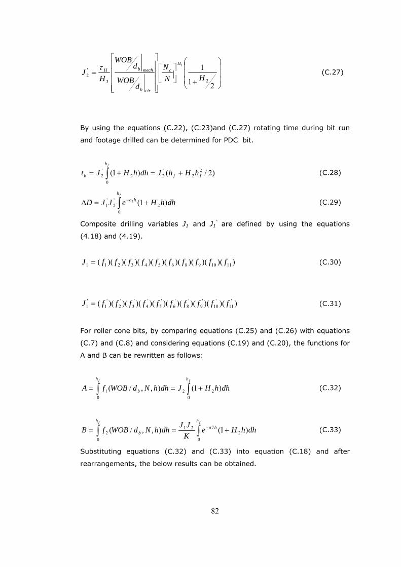
⎟⎟⎟
⎠
⎞
⎜⎜⎜
⎝
⎛
+⎥⎦⎤
⎢⎣⎡
⎥⎥⎥⎥
⎦
⎤
⎢⎢⎢⎢
⎣
⎡
=
21
123
'2
1
HNN
dWOB
dWOB
HJ
Hc
cirb
mechbHτ (C.27)
By using the equations (C.22), (C.23)and (C.27) rotating time during bit run
and footage drilled can be determined for PDC bit.
)2/()1( 22
'2
02
'2 ff
h
b hHhJdhhHJtf
+=+= ∫ (C.28)
dhhHeJJDfh
ha )1(0
2'2
'1
7∫ +=Δ − (C.29)
Composite drilling variables J1 and J1’ are defined by using the equations
(4.18) and (4.19).
))()()()()()()()()(( 1110986543211 ffffffffffJ = (C.30)
))()()()()()()()()(( '11
'10
'9
'8
'6
'5
'4
'3
'2
'1
'1 ffffffffffJ = (C.31)
For roller cone bits, by comparing equations (C.25) and (C.26) with equations
(C.7) and (C.8) and considering equations (C.19) and (C.20), the functions for
A and B can be rewritten as follows:
dhhHJdhhNdWOBfAff h
b
h
)1(),,/(0
220
1 ∫∫ +== (C.32)
dhhHeKJJdhhNdWOBfB
ff hha
b
h
)1(),,/(0
2721
02 ∫∫ +== − (C.33)
Substituting equations (C.32) and (C.33) into equation (C.18) and after
rearrangements, the below results can be obtained.
82
∫
∫
+
⎪⎪⎭
⎪⎪⎬
⎫
⎪⎪⎩
⎪⎪⎨
⎧
−
⎥⎥⎥⎥
⎦
⎤
⎢⎢⎢⎢
⎣
⎡ −⎟⎠⎞⎜
⎝⎛
⎥⎥⎥
⎦
⎤
⎢⎢⎢
⎣
⎡⎟⎠⎞
⎜⎝⎛Δ
+−=
⎥⎦⎤
⎢⎣⎡∂
∂⎥⎦⎤
⎢⎣⎡∂
∂
−f
f
hha
b
bb
a
ba
h
b
b
dhhHed
WOBd
WOBd
WOBa
dWOB
NKD
dhhH
dWOB
Bd
WOB
A
02
7max5
56
02
)1(14100
)1(
(C.34)
∫
∫
+−⎥⎥⎥
⎦
⎤
⎢⎢⎢
⎣
⎡⎟⎠⎞
⎜⎝⎛Δ
+−=
∂∂∂∂
−f
f
hha
a
ba
h
dhhHead
WOBN
KD
dhhHH
NBNA
02
76
56
021
)1()1(4100
)1( (C.35)
Comparing equations (C.34) and (C.35), following equation can be obtained.
⎥⎦⎤
⎢⎣⎡ −⎟
⎠⎞⎜
⎝⎛−
=−
bbb
b
dWOB
dWOBad
WOB
dWOB
aHH
max5
61
1 (C.36)
Solving equation C.36 for WOB/db,the optimum weight on bit can be derived as
follow.
For roller cone bits
615
max15
aHad
WOBHa
dWOB b
optb +
⎟⎠⎞⎜
⎝⎛
=⎟⎠⎞⎜
⎝⎛ (C.37)
For PDC bits, the same process should be repeated to derive optimum weight
on bit by using equations (C.28) and (C.29).The equation is represented as
follow.
61
51
aH
dWOB
dWOBaH
dWOB cirbcb
optb −
⎥⎦⎤
⎢⎣⎡
⎟⎠⎞⎜
⎝⎛+⎟
⎠⎞⎜
⎝⎛
=⎟⎠⎞⎜
⎝⎛ (C.38)
83


![Deep Directional Statistics: Pose Estimation with ......Deep Directional Statistics: Pose Estimation with Uncertainty Quantification Sergey Prokudin1[0000−0001−6501−8234], Peter](https://img.pdfslide.net/doc/110x75/5f414669bfbaa1691e47f58b/deep-directional-statistics-pose-estimation-with-deep-directional-statistics.jpg)