Embed Size (px)
Citation preview
Rational Expression Simplification
with Polynomial Side Relations
by
Roman PearceB.Sc., Simon Fraser University, 2001
A THESIS SUBMITTED IN PARTIAL FULFILLMENTOF THE REQUIREMENTS FOR THE DEGREE OF
MASTER OF SCIENCE
In the Departmentof
Mathematics
c© Roman Pearce 2005SIMON FRASER UNIVERSITY
August 2005
All rights reserved. This work may not be reproducedin whole or in part, by photocopy or other means,
without the permission of the author.
Approval
Name: Roman Pearce
Degree: Master of Science
Title of Thesis: Rational Expression Simplificationwith Polynomial Side Relations
Examining Committee: Dr. Petr LisonekAssistant ProfessorChair
Dr. Michael MonaganAssociate ProfessorSenior Supervisor
Dr. Imin ChenAssistant Professor
Dr. Marc RybowiczExternal Examinerl’Universite de Limoges33, rue Francois Mitterrand87032 Limoges Cedex 01, France
Date Approved:
ii
Abstract
The goal of this thesis is to develop generic algorithms for computing in polyno-mial quotient rings and their fields of fractions. We present two algorithms forsimplifying rational expressions over k[x1, . . . , xn]/I. The first algorithm usesGroebner bases for modules to compute an equivalent expression whose largestterm is minimal with respect to a given monomial order. The second algorithmsolves systems of linear equations to find equivalent expressions and conducts abrute force search to find an expression of minimal total degree.
iii

Dedication
To my wife Sarah,
whose tolerance and support exceeded all reasonable bounds.
iv
Acknowledgements
I would like to thank my supervisor Dr. Michael Monagan. His insights andoutlook have influenced me far more than I would care to admit, and all for thebetter. The algorithm of Section 2.5 and the suggestion to use ideal quotientsare his. I am also indebted for his unwaivering support and seemingly infinitepatience, even when I didn’t deserve it.
v
Contents
Approval Page ii
Abstract iii
Dedication iv
Acknowledgements v
Table of Contents vi
1 Preliminaries 11.1 Introduction . . . . . . . . . . . . . . . . . . . . . . . . . . . . . . 11.2 Definitions . . . . . . . . . . . . . . . . . . . . . . . . . . . . . . . 21.3 Grobner Bases . . . . . . . . . . . . . . . . . . . . . . . . . . . . 41.4 Ideal Operations . . . . . . . . . . . . . . . . . . . . . . . . . . . 101.5 Homogenization . . . . . . . . . . . . . . . . . . . . . . . . . . . . 121.6 Modules . . . . . . . . . . . . . . . . . . . . . . . . . . . . . . . . 14
2 Quotient Rings 182.1 Arithmetic in k[x1, . . . , xn]/I . . . . . . . . . . . . . . . . . . . . 182.2 Polynomial Division . . . . . . . . . . . . . . . . . . . . . . . . . 192.3 Rational Expressions I . . . . . . . . . . . . . . . . . . . . . . . . 212.4 Rational Expressions II . . . . . . . . . . . . . . . . . . . . . . . 242.5 Rational Expressions III . . . . . . . . . . . . . . . . . . . . . . . 28
A Implementation 32A.1 PolynomialIdeals in Maple 10 . . . . . . . . . . . . . . . . . . . . 32A.2 Inverses and Exact Division . . . . . . . . . . . . . . . . . . . . . 36A.3 Rational Expression Simplification . . . . . . . . . . . . . . . . . 38
vi

Chapter 1
Preliminaries
1.1 Introduction
The manipulation of polynomials is a fundamental goal of computer algebra.It was the purpose for which many of the first computer algebra systems werewritten, and it remains an area of active research today. Presently, we havegood algorithms to factor polynomials and simplify rational expressions overthe rational numbers, finite fields, and over algebraic number fields.
The direction of our work has been somewhat different. Our goal is to developgeneric algorithms for polynomial division and rational expression simplificationin the presence of algebraic side relations. More precisely, we want to computein polynomial quotient rings and their fields of fractions.
The cornerstone of any approach will be Grobner bases. Invented by BrunoBuchberger in 1965, Grobner bases are primarily used for ideal-theoretic com-putations and for simplifying elements of a quotient ring to a canonical form.They can also be used to solve linear equations modulo an ideal, which we willuse to invert elements and perform exact division.
In this thesis we present two solutions to the problem of rational expres-sion simplification. This is a problem which arises quite naturally in computeralgebra, often in relatively simple contexts. Consider the expression below.
sin(x) + 1sin4(x)− cos4(x) + sin(x)
This is a rational expression in sin(x) and cos(x), where the functions them-selves satisfy the polynomial relation sin(x)2 + cos(x)2 = 1. We would like tosimplify the fraction so as to minimize the total degree of both the numera-tor and denominator in the result. We demonstrate using an ad-hoc method.
1
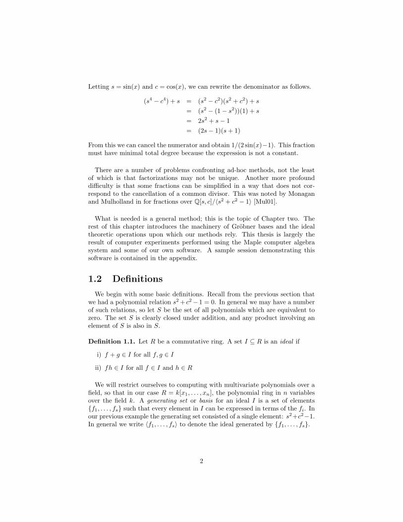
Letting s = sin(x) and c = cos(x), we can rewrite the denominator as follows.
(s4 − c4) + s = (s2 − c2)(s2 + c2) + s
= (s2 − (1− s2))(1) + s
= 2s2 + s− 1= (2s− 1)(s + 1)
From this we can cancel the numerator and obtain 1/(2 sin(x)−1). This fractionmust have minimal total degree because the expression is not a constant.
There are a number of problems confronting ad-hoc methods, not the leastof which is that factorizations may not be unique. Another more profounddifficulty is that some fractions can be simplified in a way that does not cor-respond to the cancellation of a common divisor. This was noted by Monaganand Mulholland in for fractions over Q[s, c]/〈s2 + c2 − 1〉 [Mul01].
What is needed is a general method; this is the topic of Chapter two. Therest of this chapter introduces the machinery of Grobner bases and the idealtheoretic operations upon which our methods rely. This thesis is largely theresult of computer experiments performed using the Maple computer algebrasystem and some of our own software. A sample session demonstrating thissoftware is contained in the appendix.
1.2 Definitions
We begin with some basic definitions. Recall from the previous section thatwe had a polynomial relation s2 + c2− 1 = 0. In general we may have a numberof such relations, so let S be the set of all polynomials which are equivalent tozero. The set S is clearly closed under addition, and any product involving anelement of S is also in S.
Definition 1.1. Let R be a commutative ring. A set I ⊆ R is an ideal if
i) f + g ∈ I for all f, g ∈ I
ii) fh ∈ I for all f ∈ I and h ∈ R
We will restrict ourselves to computing with multivariate polynomials over afield, so that in our case R = k[x1, . . . , xn], the polynomial ring in n variablesover the field k. A generating set or basis for an ideal I is a set of elements{f1, . . . , fs} such that every element in I can be expressed in terms of the fi. Inour previous example the generating set consisted of a single element: s2+c2−1.In general we write 〈f1, . . . , fs〉 to denote the ideal generated by {f1, . . . , fs}.
2
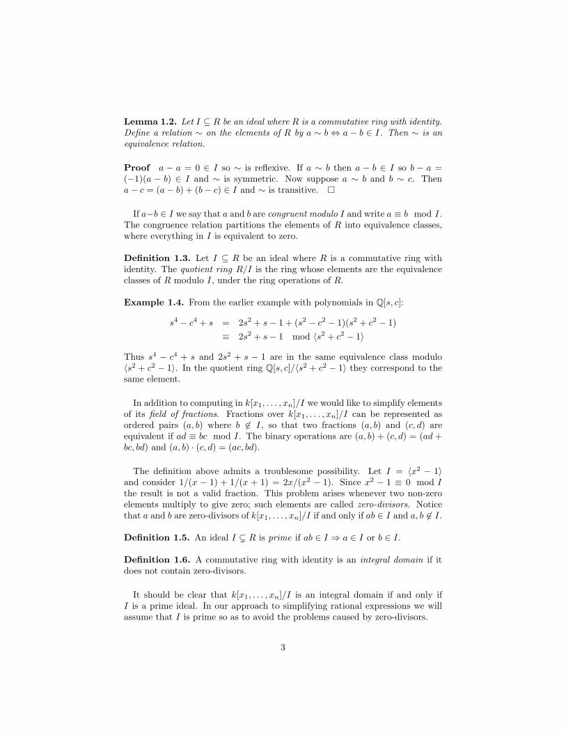
Lemma 1.2. Let I ⊆ R be an ideal where R is a commutative ring with identity.Define a relation ∼ on the elements of R by a ∼ b ⇔ a− b ∈ I. Then ∼ is anequivalence relation.
Proof a − a = 0 ∈ I so ∼ is reflexive. If a ∼ b then a − b ∈ I so b − a =(−1)(a − b) ∈ I and ∼ is symmetric. Now suppose a ∼ b and b ∼ c. Thena− c = (a− b) + (b− c) ∈ I and ∼ is transitive. �
If a−b ∈ I we say that a and b are congruent modulo I and write a ≡ b mod I.The congruence relation partitions the elements of R into equivalence classes,where everything in I is equivalent to zero.
Definition 1.3. Let I ⊆ R be an ideal where R is a commutative ring withidentity. The quotient ring R/I is the ring whose elements are the equivalenceclasses of R modulo I, under the ring operations of R.
Example 1.4. From the earlier example with polynomials in Q[s, c]:
s4 − c4 + s = 2s2 + s− 1 + (s2 − c2 − 1)(s2 + c2 − 1)≡ 2s2 + s− 1 mod 〈s2 + c2 − 1〉
Thus s4 − c4 + s and 2s2 + s − 1 are in the same equivalence class modulo〈s2 + c2 − 1〉. In the quotient ring Q[s, c]/〈s2 + c2 − 1〉 they correspond to thesame element.
In addition to computing in k[x1, . . . , xn]/I we would like to simplify elementsof its field of fractions. Fractions over k[x1, . . . , xn]/I can be represented asordered pairs (a, b) where b 6∈ I, so that two fractions (a, b) and (c, d) areequivalent if ad ≡ bc mod I. The binary operations are (a, b) + (c, d) = (ad +bc, bd) and (a, b) · (c, d) = (ac, bd).
The definition above admits a troublesome possibility. Let I = 〈x2 − 1〉and consider 1/(x − 1) + 1/(x + 1) = 2x/(x2 − 1). Since x2 − 1 ≡ 0 mod Ithe result is not a valid fraction. This problem arises whenever two non-zeroelements multiply to give zero; such elements are called zero-divisors. Noticethat a and b are zero-divisors of k[x1, . . . , xn]/I if and only if ab ∈ I and a, b 6∈ I.
Definition 1.5. An ideal I ( R is prime if ab ∈ I ⇒ a ∈ I or b ∈ I.
Definition 1.6. A commutative ring with identity is an integral domain if itdoes not contain zero-divisors.
It should be clear that k[x1, . . . , xn]/I is an integral domain if and only ifI is a prime ideal. In our approach to simplifying rational expressions we willassume that I is prime so as to avoid the problems caused by zero-divisors.
3
1.3 Grobner Bases
Grobner bases are a fundamental tool of algebraic geometry. They generalizethe ideas behind the Euclidean algorithm and Gaussian elimination to systemsof multivariate polynomials and provide canonical representatives for elementsof a quotient ring. This allows us simplify expressions and detect zero.
A key ingredient of linear algebra and univariate polynomial computationsis that an order is imposed on the monomials which may appear. In Gaussianelimination the monomials are variables, ordered a priori or incrementally bya pivoting strategy. In the Euclidean algorithm powers of a single variable areordered by their degree. The definition below generalizes both of these concepts.
Definition 1.7. A monomial order is a relation < such that
i) < is a total order on the monomials of k[x1, . . . , xn]
ii) a < b =⇒ ac < bc for monomials a, b, and c
iii) 1 is the smallest monomial under <
Example 1.8. In lexicographic order with x1 > x2 > · · · > xn monomials arecompared first by their degree in x1, then by their degree in x2, and so on,continuing as long as there is a tie.
Example 1.9. In graded lexicographic order with x1 > x2 > · · · > xn mono-mials are first compared by their total degree with ties broken by lexicographicorder as above. To illustrate we have written the terms of the polynomial belowin descending graded-lexicographic order with x > y > z.
f(x, y, z) = x3 + x2z + xy2 + x2 + xy + xz + y2 + x + y + z + 1
Example 1.10. In graded-reverse lexicographic order with x1 > x2 > · · · > xn
monomials are again compared first by their total degree but ties are brokenby preferring monomials with least degree in the smallest variables. We haverewritten the polynomial above so that its terms are in descending graded-reverse lexicographic order with x > y > z.
f(x, y, z) = x3 + xy2 + x2z + x2 + xy + y2 + xz + x + y + z + 1
Observe that x3 is again the largest monomial, only this time because its degreein z and then y is smallest among its competitors. For the same reason, xy2 isnow greater than x2z and y2 is greater than xz.
Example 1.11. In an elimination order with {x1, . . . , xi−1} � {xi, . . . , xn}monomials are first compared using a monomial order on {x1, . . . , xi−1}, withties broken by a second order on {xi, . . . , xn}. As a result, the monomials
4
containing {x1, . . . , xi−1} are all greater than the monomials involving only{xi, . . . , xn}. Elimination orders can also have multiple groups of variables.The extreme case where {x1} � {x2} � · · · � {xn} is lexicographic order.
Definition 1.12. Let f ∈ k[x1, . . . , xn]. The leading term of f , denoted LT(f),is the term whose monomial is greatest with respect to a monomial order. Thecoefficient and monomial of this term are called the leading coefficient and lead-ing monomial respectively.
Monomial orders lead to a natural generalization of polynomial division. Herea single polynomial is divided by a set of polynomials producing a remainderand optionally a sequence of quotients. When our choice of monomial order isclear we write f ÷ G → r to denote the division of a polynomial f by a list ofpolynomials G producing a remainder r.
Algorithm 1.13 (The Division Algorithm).Input a polynomial f , a list of polynomials G, a monomial order <Output a polynomial r where no term of r is divisible by an LT(Gi),
(optionally) a list of polynomials Q with f −∑|G|
i=1 QiGi = r(p, r)← (f, 0)Q← (0, . . . , 0)while p 6= 0 do
select the first Gi where LT(Gi) divides LT(p)if no such Gi exists move LT(p) to the remainder
r ← r + LT(p)p← p− LT(p)
else cancel LT(p) using Gi
Qi ← Qi + (LT(p)/LT(Gi))p← p− (LT(p)/LT(Gi))Gi
end ifend loopreturn r, Q
We would like to use the division algorithm to test for membership in an ideal,but doing so poses a problem. Consider I = 〈x2 + 1, xy + 1〉. The polynomialx(xy+1)−y(x2 +1) = x−y is clearly a member of the ideal, however it can notbe reduced by either x2 + 1 or xy + 1 using any monomial order. The problemis remedied by the following condition.
Definition 1.14. Let I ⊆ k[x1, . . . , xn] be an ideal and let < be a monomialorder. A set G is a Grobner basis for I with respect to < if for every f ∈ I,LT(f) is divisible by LT(g) for some g ∈ G.
Example 1.15. Let I = 〈x3−1, x2−x〉 in Q[x]. From the Extended Euclideanalgorithm we obtain gcd(x3−1, x2−x) = (1)(x3−1)−(x+1)(x2−x) = x−1 ∈ I.
5
Every element of I is of the form p(x3−1)+q(x2−x) which is divisible by x−1so I = 〈x− 1〉 and {x− 1} is a Grobner basis.
Theorem 1.16. Let G be a Grobner basis for I ⊆ k[x1, . . . , xn]. Then
i) f ÷G→ r implies f ≡ r mod I
ii) f ≡ g mod I and f ÷G→ r implies g ÷G→ r
Proof (i) By Algorithm 1.13 we have f − r =∑|G|
i=1 QiGi ≡ 0 mod I. (ii) Iff ÷G→ r and g ÷G→ r′ then no term of r (respectively r′) is divisible by aleading term of G. Then no term of r − r′ is divisible by a leading term of G,and since r − r′ ∈ I and G is a Grobner basis this implies r − r′ = 0. �
Corollary 1.17.
i) f ÷G→ 0 if and only if f ∈ I
ii) if f ÷G→ r then the remainder r is unique
For a given monomial order, Theorem 1.16 associates each equivalence classof k[x1, . . . , xn]/I with a unique remainder, called a normal form, which can becomputed by division with a Grobner basis for I. Thus we can perform addi-tion and multiplication in k[x1, . . . , xn]/I using the operations of k[x1, . . . , xn],followed by a reduction to the normal form.
Having demonstrated the usefulness of Grobner bases we turn now to theirconstruction. Previously we discovered x − y ∈ 〈x2 + 1, xy + 1〉 by inducing acancellation of the leading terms of x2 + 1 and xy + 1. This is called a syzygy,and to compute a Grobner basis for an arbitrary ideal it will suffice to computethese syzygies one at a time and add them, when necessary, to the generating set.
Definition 1.18. Let f and g be polynomials and let < be a monomial order.The syzygy polynomial of f and g is
S(f, g) =LT(g)f − LT(f)ggcd(LT(f),LT(g))
Theorem 1.19 (Buchberger’s Syzygy Criterion). Let I be an ideal withgenerating set G and let < be a monomial order. G is a Grobner basis for Iwith respect to < if and only if S(f, g)÷G→ 0 for all f, g ∈ G.
Proof See [Cox96].
6
We present a crude version of Buchberger’s algorithm based on Theorem 1.19.The algorithm terminates when S(f, g)÷G→ 0 has been verified for all f, g ∈ G.This is guaranteed to happen by the ascending chain condition; every strictlyincreasing sequence of ideals in k[x1, . . . , xn] is finite. Observe that when a non-zero remainder r is added to G the ideal of leading monomials of G is strictlyenlarged. The ACC also implies that every ideal of k[x1, . . . , xn] has a finite setof generators, so that Algorithm 1.20 implies the existence of Grobner bases.
Algorithm 1.20 (Buchberger’s Algorithm).Input a set of generators F , a monomial order <Output a Grobner basis G with respect to <G← FP ← {(f, g) | f, g ∈ F}while |P | > 0 do
select a pair (f, g) ∈ PP ← P \ {(f, g)}r ← S(f, g)÷Gif r 6= 0
P ← P ∪ {(h, r) | h ∈ G}G← G ∪ {r}
end ifend loopreturn G
Example 1.21. We compute a Grobner basis for 〈xy + 1, x2 + 1〉 ⊆ Q[x, y]using lexicographic order with x > y. Our initial basis consists of just thesepolynomials, but we have a syzygy.
S(xy + 1, x2 + 1) = x(xy + 1)− y(x2 + 1) = x− y
This polynomial can not be reduced by either x2 + 1 or xy + 1 so we add it tothe basis unchanged and two new syzygies are created.
S(x2 + 1, x− y) = (x2 + 1)− x(x− y) = xy + 1
S(xy + 1, x− y) = (xy + 1)− y(x− y) = y2 + 1
The first polynomial is already in the basis and thus reduces to zero. The secondone doesn’t reduce, so it is added to the basis and its syzygies are constructed.
S(x2 + 1, y2 + 1) = y2(x2 + 1)− x2(y2 + 1) = −x2 + y2
S(xy + 1, y2 + 1) = y(xy + 1)− x(y2 + 1) = −x + y
S(x− y, y2 + 1) = y2(x− y)− x(y2 + 1) = −x− y3
One can easily verify that all of these syzygies reduce to zero. The algorithmterminates with {xy + 1, x2 + 1, x− y, y2 + 1} which is a Grobner basis.
7
Observe that the initial generators xy + 1 and x2 + 1 in Example 1.21 are nolonger needed in the final Grobner basis. To see this, we can sort the basis intodescending order and divide each element by its successors using Algorithm 1.13.We find that x2 + 1 = x(x− y) + (xy + 1) and xy + 1 = y(x− y) + (y2 + 1), so{x− y, y2 + 1} is also a Grobner basis.
Definition 1.22. Let G be a Grobner basis, G is reduced if 0 6∈ G and eachg ∈ G is in normal form with respect to G \ {g}.
A particularly useful property of reduced Grobner bases is that their elementsare unique up to a constant multiple [Cox96]. Starting from the output ofBuchberger’s algorithm one can construct a reduced Grobner basis by dividingas above, although more efficient methods exist. Some variants of Buchberger’salgorithm also partially reduce the basis as new polynomials are added [Geb88].
With regards to a practical implementation Algorithm 1.20 is dreadfully slow.In practice it is not necessary to consider every S(f, g) and criteria have beendeveloped to omit superfluous ones [Buc79][Geb88]. Still the vast majorityof time in Buchberger’s algorithm is spent reducing syzygies to zero [Buc85].Subsequent algorithms by J.C. Faugere improve on this by considering severalsyzygies at once [Fau99][Fau02].
One redeeming property of Algorithm 1.20 is that we can easily modify it toexpress the resulting Grobner basis elements in terms of the initial generators.The idea is to attach a vector C to each g ∈ G with the property that
g =|F |∑i=1
CiFi
Whenever polynomial arithmetic is performed, the vectors are updated with theanalogous operation. We illustrate the technique by repeating Example 1.21.
Example 1.23. Let F = [xy + 1, x2 + 1] ⊂ Q[x, y] be our generating set, againusing lexicographic order with x > y. We begin by attaching the identity vectors[1, 0] and [0, 1] to xy + 1 and x2 + 1. The first syzygy
S(xy + 1, x2 + 1) = x(xy + 1)− y(x2 + 1) = x− y
is assigned the vector x[1, 0]− y[0, 1] = [x,−y]. Continuing, we assign
S(xy + 1, x− y) = y2 + 1 1[1, 0]− y[x,−y] = [1− xy, y2]
S(x2 + 1, x− y) = xy + 1 1[0, 1]− x[x,−y] = [−x2, 1 + xy]
Were we to reduce these polynomials we would have to update their vectors inAlgorithm 1.13 as well, but for now we are done. The remaining syzygies all
8
reduce to zero and [xy + 1, x2 + 1, x − y, y2 + 1] is a Grobner basis. From thevectors we obtain the following relations.
xy + 1 = 1 (xy + 1) + 0 (x2 + 1)x2 + 1 = 0 (xy + 1) + 1 (x2 + 1)x− y = x (xy + 1)− y (x2 + 1)
y2 + 1 = (1− xy) (xy + 1) + y2 (x2 + 1)
1.4 Ideal Operations
In addition to membership testing, Grobner bases also can be used to computemany ideal-theoretic operations. Because surveys of this area usually constitutea volume, we present a minimum amount of material and defer to [Cox96] and[BW93] for additional treatment. We begin with the intersection of an idealand a subring of k[x1, . . . , xn].
Theorem 1.24 (The Elimination Theorem). Let I ⊆ k[x1, . . . , xn] be anideal and let G be a Grobner basis for I with respect to an elimination order <with {x1, . . . , xi−1} � {xi, . . . , xn}. Then G ∩ k[xi, . . . , xn] is a Grobner basisfor I ∩ k[xi, . . . , xn] under the restriction of < to {xi, . . . , xn}.
Proof Note that G ∩ k[xi, . . . , xn] ⊂ I ∩ k[xi, . . . , xn] since G ⊂ I. Now forf ∈ I ∩ k[xi, . . . , xn] we have f ÷ G → 0 under < but no term of f contains{x1, . . . , xi−1} so only elements of G∩ k[xi, . . . , xn] can be used in the division.The same argument applied to {S(gi, gj) : gi, gj ∈ G∩ k[xi, . . . , xn]} shows thatG ∩ k[xi, . . . , xn] is a Grobner basis. �
Example 1.25. In Example 1.21 we found that {x2 + 1, xy + 1, y − x, y2 + 1}is a Grobner basis for I = 〈x2 + 1, xy + 1〉 ⊂ Q[x, y] under lexicographic orderwith x > y. Since this is an elimination order I ∩Q[y] = 〈y2 + 1〉.
Definition 1.26. Let I = 〈f1, . . . , fs〉 and J = 〈g1, . . . , gt〉. Then
i) The ideal sum I + J = 〈f1, . . . , fs, g1, . . . , gt〉.
ii) The ideal product IJ = 〈f1g1, . . . , figj , . . . , fsgt〉
iii) The intersection I ∩ J = {f : f ∈ I and f ∈ J}
A clever trick reduces the computation of ideal intersections to the subringintersection of Theorem 1.24. Let I ⊆ k[x1, . . . , xn] be an ideal and let t be anextra variable. We let tI denote the ideal product of 〈t〉 and I in k[x1, . . . , xn, t].
Lemma 1.27. Let I and J be ideals of k[x1, . . . , xn]. Then I ∩ J =(tI + (1− t)J) ∩ k[x1, . . . , xn].
9
Proof Suppose f ∈ I ∩ J ⊆ k[x1, . . . , xn]. Then tf ∈ tI and (1 − t)f ∈(1 − t)J so f = tf + (1 − t)f ∈ (tI + (1 − t)J) ∩ k[x1, . . . , xn]. Now letf ∈ (tI + (1 − t)J) ∩ k[x1, . . . , xn]. Then 〈tf〉 ⊆ (tI + (1 − t)J) so we canadd 〈1 − t〉 to both sides and obtain f ∈ 〈tf, 1 − t〉 ⊆ I + 〈1 − t〉 and intersectwith k[x1, . . . , xn] to get f ∈ I. A similar argument shows f ∈ J . �
Example 1.28. Let I = 〈x − 1, y − 1〉 and J = 〈x − 1, y + 1〉. We eliminatet from {t(x − 1), t(y − 1), (1 − t)(x − 1), (1 − t)(y + 1)} using a lexicographicGrobner basis with t > x > y. The Grobner basis is {y2 − 1, x− 1, 2t− y − 1}so I ∩ J = 〈y2 − 1, x− 1〉.
The most important task of this section is to describe the quotient operationfor ideals. Analogous to cancelling out a GCD, it forms the basis of one of ourmethods for simplifying rational expressions over k[x1, . . . , xn]/I.
Definition 1.29. Let I, J ⊆ k[x1, . . . , xn] be ideals. The ideal quotient I : J isthe set {f ∈ k[x1, . . . , xn] : fh ∈ I for all h ∈ J}.
We show that I : J is an ideal. Note that it trivially contains I. If f, g ∈ I : Jand h ∈ J then (f + g)h = fh + gh ∈ I so (f + g) ∈ I : J . Likewise if f ∈ I : J ,h ∈ J and g ∈ k[x1, . . . , xn] then fgh ∈ I since fh ∈ I, so fg ∈ I : J .
Example 1.30. Let I = 〈x2 − y2〉 and J = 〈x− y〉. Then I : J = 〈x + y〉.
Example 1.31. Let f, g ∈ k[x]. The quotient 〈f〉 : 〈g〉 contains all polynomialswhose product with g is a multiple of f . In particular, a minimal element islcm(f, g)/g = f/ gcd(f, g) which also generates the ideal.
The properties below are noted by Cox et al [Cox96]. The third propertycombined with the subsequent lemma provides an algorithm to compute I : J .
Lemma 1.32. Let I, J , and K be ideals of k[x1, . . . , xn]. Then
i) I : J = k[x1, . . . , xn] if and only if J ⊆ I
ii) IJ ⊆ K if and only if I ⊆ K : J
iii) I : (∑s
i=1 Ji) =⋂s
i=1(I : Ji)
Proof See [Cox96].
Lemma 1.33. Let G be a Grobner basis for I ∩ 〈f〉. Then {g/f : g ∈ G} is aGrobner basis for I : 〈f〉 with respect to the same monomial order.
10

Proof First observe gi ∈ 〈f〉 so each gi/f is a polynomial. Then gi/f ∈ I : 〈f〉since (gi/f)f = gi ∈ I. Now let h ∈ I : 〈f〉. We know LT(fh) is divisible bysome LT(gi) since {g1, . . . , gt} is a Grobner basis. Then LT(h) is divisible byLT(gi/f), and since h was arbitrary {g1/f, . . . , gt/f} is a Grobner basis. �
Example 1.34. Let I = 〈x2, y2 − 1〉 and J = 〈x, y − 1〉 in Q[x, y]. ThenI ∩ 〈x〉 = 〈x2, x(y2 − 1)〉 and I ∩ 〈y − 1〉 = 〈x2(y − 1), y2 − 1〉 so
I : J = (I : 〈x〉) ∩ (I : 〈y − 1〉)= 〈x, y2 − 1〉 ∩ 〈x2, y + 1〉= 〈x2, x(y + 1), y2 − 1〉
1.5 Homogenization
Next we present a few interesting results about homogeneous Grobner basesfrom [Fro97]. A generalization to arbitrary gradings appears in §10.2 of [BW93].
Definition 1.35. A polynomial f ∈ k[x1, . . . , xn] is homogeneous if all of itsnon-zero terms have the same total degree.
Lemma 1.36. Let f and G = [g1, . . . , gt] be homogeneous polynomials. If wecompute f ÷ G → r using Algorithm 1.13, then the remainder r and all of thequotients are also homogeneous.
Proof Upon entering the main loop p (which is initially f) is homogeneousand we take one of two actions. If LT(p) is divisible by some LT(gi) then wesubtract pnew ← p− (LT(p)/LT(gi))gi. Since gi is homogeneous pnew is homo-geneous and deg(pnew) = deg(p) if pnew 6= 0. Otherwise we move the leadingterm of p to the remainder r. Because the degree of p is invariant while p 6= 0the terms of r all have degree deg(f). Similarly, the non-zero terms of eachquotient Qi must have degree deg(f)− deg(gi). �
Lemma 1.37. Let I be an ideal generated by homogeneous polynomials. Thena reduced Grobner basis for I with respect to any monomial order consists ofhomogeneous polynomials.
Proof Observe that syzygies of homogeneous polynomials are homogeneousand by Lemma 1.36 so are their remainders. Thus the Buchberger algorithmadds only homogeneous polynomials to the generating set. To reduce a Grobnerbasis it suffices to divide each g ∈ G by G \ {g} and remove zero. Again byLemma 1.36 the result is a set of homogeneous polynomials. �
An ideal with homogeneous generators is said to be homogeneous also. Notethat the class of homogeneous ideals is closed under the operations of Section 1.4,
11
although we have omitted some of the requisite details.
Definition 1.38. Let f ∈ k[x1, . . . , xn] and let y be a new variable. The ho-mogenization of f in y is the polynomial f (y) = ydeg(f)f(x1/y, . . . , xn/y).
Example 1.39. Let f = x3 + x + 1 ∈ Q[x]. We introduce y to homogenize f .Applying Definition 1.38 we obtain f (y) = x3 + xy2 + y3.
Homogenization is an injective map from k[x1, . . . , xn] to k[x1, . . . , xn, y] whichcan be inverted by evaluating y = 1. It is not a ring homomorphism since(f + g)(y) 6= f (y) + g(y) when f and g have different total degree. Nevertheless,using Grobner basis theory we can recover some of the results for homogeneouspolynomials, provided we accept the following condition.
Definition 1.40. Let < be a monomial order on k[x1, . . . , xn] and let y bea new variable. We say that <′ is a good extension of < to k[x1, . . . , xn, y] ifLT<(f) = LT<′(f (y)) for all f ∈ k[x1, . . . , xn].
Example 1.41. Let < and <′ denote graded lexicographic order with x > yand x > y > z respectively. We show that <′ is not a good extension of <. Letf = x + y2. Then LT<(f) = y2 but LT<′(f (z)) = LT<′(xz + y2) = xz.
Example 1.42. Let < and <′ denote graded reverse lexicographic order withx1 > x2 > . . . xn and x1 > x2 > · · · > xn > y respectively. We show that<′ is a good extension of <. If f (y) is the homogenization of f ∈ k[x1, . . . , xn]then all of its terms have degree deg(f) and to compute LT<′(f (y)) we firstselect the terms with lowest degree in y. These terms have degree zero in y anddegree deg(f) in {x1, . . . , xn} so they are initially selected by < as well. ThenLT<′(f (y)) = LT<(f) since subsequent ties are broken in an identical manner.
Not all monomial orders have good extensions. In fact, LT<(f) = LT<′(f (y))requires deg(LT<(f)) = deg(f) for all f so only graded orders can be extended.The purpose of good extensions is simple: as we will see in the following theo-rem, the property of being a Grobner basis is preserved under homogenizationand dehomogenization. This has numerous applications in projective geometry,see [Cox96] for examples.
Definition 1.43. Let I ⊆ k[x1, . . . , xn] be an ideal. The homogenization of Iin y is the ideal I(y) generated by {f (y) : f ∈ I} in k[x1, . . . , xn, y].
Example 1.44. Let I = 〈y − 1, xy − 1〉. If we homogenize y − 1 and xy − 1using a new variable z we obtain I ′ = 〈y − z, xz − z2〉. However x − 1 ∈ I sox− z ∈ I(z) but x− z 6∈ I ′. This shows that we can not simply homogenize thegenerators of I to obtain I(z).
12
Theorem 1.45. Let I ⊆ k[x1, . . . , xn] be an ideal, and let G be a reducedGrobner basis for I with respect to a monomial order <. If y is a new variableand <′ is a good extension of < to {x1, . . . , xn, y}, then G(y) = {g(y) : g ∈ G}is a reduced Grobner basis for I(y) under <′.
Proof See [Fro97].
Example 1.46. Let I = 〈y − 1, xy − 1〉 as in Example 1.44. We homogenizeI using graded reverse lexicographic order with x > y > z, which is a goodextension of the same order with x > y. A reduced Grobner basis for I is{y−1, x−1} so a reduced Grobner basis for I(z) is {y−z, x−z} by Theorem 1.45.
1.6 Modules
For our final section of preliminary material, we introduce Grobner bases formodules. Modules over rings are similar to vector spaces over fields, althoughour presentation focuses entirely on developing Grobner basis techniques. Fora more comprehensive treatment of modules refer to [Cox98].
Definition 1.47. Let R be a ring with unity. A module over R or R-module is aset M together with operations for addition and scalar multiplication satisfying
i) (M,+) is an Abelian group
ii) 1f = f for all f ∈M
iii) (ab)f = a(bf) ∈M for all a, b ∈ R and f ∈M
iv) (a + b)f = af + bf for all a, b ∈ R and f ∈M
v) a(f + g) = af + ag for all a ∈ R and f, g ∈M
When R is not commutative the definition above is that of a left R-module,however we are only concerned with the case R = k[x1, . . . , xn]. In fact, we willonly consider modules which are a subset of Rm. These are submodules of Rm,since Rm is itself an R-module.
Example 1.48. Let R = k[x, y] and consider the set of all possible combinations
of[
x1
]and
[y0
]in R2. For example,
[0y
]= y
[x1
]− x
[y0
]is in the
set while[
y1
]is not. It is easy to see that this set is a module over R and
thus a submodule of R2.
Observe that submodules of R1 correspond to ideals. With this in mind it isnatural to ask whether Grobner basis techniques can be extended to work withsubmodules of Rm. The only suprising fact is that it all works out so easily.
13
Our first task is to extend monomial orders to elements of Rm. Following[Cox98], we write f ∈ Rm as a linear combination of monomials in R andstandard basis vectors ei. For example:[
x2 + y2y
]=
[x2
0
]+
[y0
]+
[02y
]= x2 e1 + y e1 + 2y e2
Then monomials of Rm are all of the form α ei where α is a monomial in R.Given a monomial order < on R = k[x1, . . . , xn] there are two natural ways toextend it to a monomial order on Rm [AL94].
Definition 1.49. Let < be a monomial order on R. The position over termmonomial order <POT is defined by a ei >POT b ej if i < j or i = j and a > b.
Definition 1.50. Let < be a monomial order on R. The term over positionmonomial order <TOP is defined by a ei >TOP b ej if a > b or a = b and i < j.
Example 1.51. Let < denote graded lexicographic order with x > y and letf = xy e1 + x2 e2 + x2 e3 =
[xy x2 x2
]T . Then the largest (or leading)monomial of f is xy e1 under <POT and x2 e2 under <TOP .
All that remains is to define division and syzygies for monomials of Rm be-fore we can run the algorithms of Section 1.3 unchanged. Quite naturally, if amonomial a ei divides b ej we expect to find q with b ej = qa ei. This is possibleif and only if i = j and a divides b in R. Similarly, one constructs syzygies byinducing a cancellation of the leading terms.
Definition 1.52. Let f, g ∈ Rm with leading terms a ei and b ej respectively.
The syzygy vector of f and g is S(f, g) =bf − ag
gcd(a, b)if i = j or 0 ∈ Rm otherwise.
Example 1.53. Let f = x e1 + e2 and g = y e1 from Example 1.48. We use<TOP extending graded lexicographic order with x > y. The leading monomialsare x e1 and y e1, so S(f, g) = yf − xg = y e2.
Example 1.54. Building on the previous example, we apply Algorithm 1.13 todivide p = (xy + y) e1 + x e2 by G = {x e1 + e2, y e1, y e2} using <TOP . Theleading monomial of p is xy e1, which is reducible by G1. We subtract
p ←[
xy + yx
]− y
[x1
]=
[y
x− y
]Since we are using a term over position order the new leading term of p is x e2.This is not divisible by any element of G, so we move it to the remainder. Thenext term of p is y e1, which is reducible by G2 so
p ←[
y−y
]−
[y0
]=
[0−y
]
14
Finally the leading term −y e2 is cancelled by adding G3 and we obtain zero.The algorithm terminates, returning the remainder r = x e2 and optionally thelist of quotients Q = [−y,−1, 1].
The characterization of Grobner bases is the same for modules as it is forpolynomial ideals, and one can show that Buchberger’s criterion (Theorem 1.19)carries over as well [Cox98]. That is, a set G is a Grobner basis if and only ifS(f, g)÷G→ 0 for all f, g ∈ G. Observe that this condition is satisfied by theset G of Example 1.54, and that it was obtained by running the Buchbergeralgorithm in Example 1.53.
Similarly Lemma 1.2, Theorem 1.16, and Corollary 1.17 all continue to holdwhen ideals I ⊆ R are replaced by modules M ⊆ Rm. As a result, Grobner basescan be used to test for membership in submodules of Rm. This is illustrated inExample 1.54, where p = (xy + y) e1 + x e2 was found not to be an element ofthe module 〈x e1 + e2, y e1〉.
We conclude with two interesting applications of Grobner bases for modules.First we show how a module computation can express a Grobner basis for anideal I ⊆ k[x1, . . . , xn] in terms of the generators, like the extended Buchbergeralgorithm of Section 1.3. We demonstrate using Example 1.23.
Example 1.55. Let F = [xy + 1, x2 + 1] and let < denote lexicographic orderwith x > y. We compute a Grobner basis for 〈F1 e1 + e2, F2 e1 + e3〉 using<POT . Our initial basis is G = {(xy + 1) e1 + e2, (x2 + 1) e1 + e3} and
S(G1, G2) = xG1 − yG2 = (x− y) e1 + x e2 + (−y) e3
Written in <POT order, the monomials are x e1, −y e1, x e2, and −y e3. Noneof them are reducible by G1 or G2, so we add this element unchanged as G3
and construct its syzygies
S(G1, G3) = G1 − yG3 = (y2 + 1) e1 + (−xy + 1) e2 + y2 e3
S(G2, G3) = G2 − xG3 = (xy + 1) e1 + (−x2) e2 + (xy + 1) e3
The latter is reducible by G1, and we add G4 = (y2+1) e1+(−xy+1) e2+y2 e3
and G5 = (−x2 − 1) e2 + (xy + 1) e3 to the basis. There are no syzygiesinvolving G5 at this point because no other Gi has a leading monomial in e2.The remaining syzygies are
S(G1, G4) = (−x + y) e1 + (x2y − x + y) e2 + (−xy2) e3
S(G2, G4) = (−x2 + y2) e1 + (x3y − x2) e2 + (−x2y2 + y2) e3
S(G3, G4) = (−x− y3) e1 + (x2y + xy2 − x) e2 + (−xy2 − y3) e3
15
all of which reduce to zero. The elements of G are written in vector form below.
G =
xy + 1
10
,
x2 + 101
,
x− yx−y
,
y2 + 11− xy
y2
,
0−x2 − 1xy + 1
Notice that the first row of G contains a Grobner basis for 〈F 〉 and the remainingrows express this basis in terms of F . Compare this to Example 1.23.
Finally we show how Grobner bases for modules can be used to computean ideal quotient I : 〈g〉. This technique (from [CT98]) is substantially fasterthan the method of Section 1.4 because it avoids the construction of I ∩ 〈g〉.By Lemma 1.33 the generators of the intersection are a factor of g larger thanthose of the quotient.
Lemma 1.56. Let R = k[x1, . . . , xn], let g ∈ R, and let I ⊆ R be an ideal. IfM = 〈Ie1, Ie2, g e1 + e2〉 ⊆ R2 then I : 〈g〉 = M ∩ e2.
Proof We first show M ∩e2 ⊆ I : 〈g〉. Every element a e1 + b e2 ∈M satisfiesa− bg ≡ 0 mod I so if b ∈M ∩ e2 then bg ≡ 0 mod I and b ∈ I : 〈g〉. Now letf ∈ I : 〈g〉. Then fg ∈ I so fg = q1f1 + · · ·+ qsfs for some {qi} ⊂ R and[
0f
]= f
[g1
]− q1
[f1
0
]− q2
[f2
0
]− . . . − qs
[fs
0
]expresses f as an element of M ∩ e2.
Example 1.57. Let I = 〈y2−x, x2−xy〉 and let g = y. We use <POT where < isgraded-reverse lexicographic order with x > y. The module 〈I e1, I e2, y e1+e2〉is generated by
G ={[
y2 − x0
],
[x2 − xy
0
],
[0
y2 − x
],
[0
x2 − xy
],
[y1
]}The pairs {S(G1, G2),S(G3, G4),S(G1, G5),S(G2, G5)} are the only syzygieswhich are not identically zero under Definition 1.52. However S(G1, G2) andS(G3, G4) must reduce to zero since {y2 − x, x2 − xy} is a Grobner basis for Iwith respect to <. Thus we compute
S(G1, G5) = (y2 − x) e1 − y(y e1 + e2) = −x e1 − y e2
S(G2, G5) = y(x2 − xy) e1 − x2(y e1 + e2) = −xy2 e1 − x2 e2
The first syzygy doesn’t reduce so it is added to the basis as G6. The secondreduces to (−xy + x) e2 following the steps below.
−xy2 e1 − x2 e2+xG1−−−−→ −x2 e1 − x2 e2
+xG2−−−−→ −xy e1 − x2 e2
+xG5−−−−→ (−x2 + x)e2
+G4−−−→ (−xy + x)e2
16
So (−xy + x) e2 is added to the basis as G7. The remaining syzygies all reduceto zero so G is a Grobner basis for 〈I e1, I e2, y e1 + e2〉 with respect to <POT .In vector form the elements of G are[
y2 − x0
],
[x2 − xy
0
],
[0
y2 − x
],
[0
x2 − xy
],
[y1
],
[−x−y
],
[0
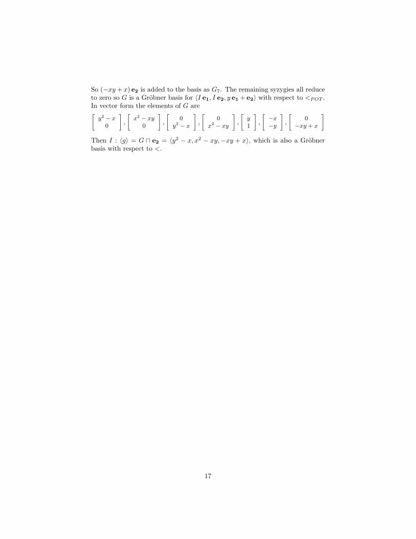
−xy + x
]Then I : 〈g〉 = G ∩ e2 = 〈y2 − x, x2 − xy,−xy + x〉, which is also a Grobnerbasis with respect to <.
17
Chapter 2
Quotient Rings
2.1 Arithmetic in k[x1, . . . , xn]/I
Recall Theorem 1.16 and Corollary 1.17; using Algorithm 1.13 and a Grobnerbasis for I we can simplify polynomials to a unique representative of their equiv-alence class modulo I. Thus we can add and multiply in k[x1, . . . , xn]/I usingthe operations of k[x1, . . . , xn], reducing to a canonical form as desired.
Example 2.1. Let I = 〈x2 + y, y2 + 1〉. We use graded lexicographic orderwith x > y. Observe that the generators of I are already a Grobner basis sinceS(x2 + y, y2 + 1) = y2(x2 + y) − x2(y2 + 1) = y3 − x2 reduces to zero. Letf = xy + 1 and let g = x + y. Then f + g = xy + x + y + 1 and
fg = x2y + xy2 + x + y
≡ (−y)y + x(−1) + x + y mod I
≡ y + 1 mod I
Our first interesting task is the computation of inverses in k[x1, . . . , xn]/I.This method is from §6.1 of [BW93]. Let f be an element of k[x1, . . . , xn]/I.Then f is invertible if and only if there exists an f−1 ∈ k[x1, . . . , xn] withff−1 ≡ 1 mod I, or equivalently 1 = ff−1 + h for some h ∈ I.
The key observation is that this is equivalent to 1 ∈ 〈f〉 + I ⊆ k[x1, . . . , xn],where 〈f〉 + I is the ideal generated by f together with the generators of I.Then {1} is a reduced Grobner basis for 〈f〉+I and we can compute the inverseusing the extended Buchberger algorithm of Section 1.3.
Example 2.2. Let I = 〈x2 + y, y2 + 1〉 and let f = x. To compute the inverseof f modulo I we run the extended Buchberger algorithm on 〈x, x2 + y, y2 + 1〉using graded lexicographic order with x > y. We assign vectors [1, 0, 0], [0, 1, 0],and [0, 0, 1] to x, x2 + y, and y2 + 1, respectively, and compute the syzygies
18
S(x, x2 + y) = x(x)− 1(x2 + y) = −y assigned [x,−1, 0]
S(−y, y2 + 1) = y(−y) + 1(y2 + 1) = 1 assigned [xy,−y, 1]
Then 1 = (xy)(x) + (−y)(x2 + y) + 1(y2 + 1). Since x2 + y and y2 + 1 are in I1 ≡ (xy)(x) mod I and x−1 = xy mod I.
2.2 Polynomial Division
We can extend the method of computing inverses in k[x1, . . . , xn]/I to describepolynomial division modulo I in general. Once again we exploit the connectionbetween representatives f ∈ k[x1, . . . , xn]/I and ideals 〈f〉 + I ⊆ k[x1, . . . , xn],which we denote by 〈f, I〉. Our approach is based on two lemmas.
Lemma 2.3. Let f be a polynomial and let I be an ideal. If {g1, . . . , gt} is aGrobner basis for 〈f, I〉 then there exist qi ∈ k[x1, . . . , xn] with gi ≡ qif mod I.
Proof The statement is actually trivial, but our goal is to compute the qi. LetI = 〈h1, . . . , hs〉. From the extended Buchberger algorithm we obtain quotientsexpressing each gi in terms of {f, h1, . . . , hs}, i.e.:
gi = qi0f + qi1h1 + qi2h2 + . . . qishs
Since all of the hi are equivalent to zero we have gi ≡ qi0f mod I. �
Example 2.4. Let f = xy + 1 and let I = 〈x2 + 1〉 ⊂ Q[x, y]. In Example 1.23we computed a Grobner basis for 〈f, I〉 using lexicographic order with x > y.We obtained the basis {xy + 1, x2 + 1, x− y, y2 + 1} and the relations
xy + 1 = 1 (xy + 1) + 0 (x2 + 1)x2 + 1 = 0 (xy + 1) + 1 (x2 + 1)x− y = x (xy + 1)− y (x2 + 1)
y2 + 1 = (1− xy) (xy + 1) + y2 (x2 + 1)
Then x− y ≡ xf mod I and y2 + 1 ≡ (1− xy)f mod I.
Example 2.5. We illustrate how to do the computation of Lemma 2.3 usingGrobner bases for modules. Let < be a monomial order and let I = 〈h1, . . . , hs〉.If we compute a Grobner basis for the module
M =⟨[
h1
0
], . . . ,
[hs
0
],
[f1
]⟩using <POT we will obtain a Grobner basis for 〈f, I〉 in the first coordinate.The second coordinate must contain the desired relations {qi}, because everyelement [a, b] ∈M satisfies a ≡ bf mod I.
19
Lemma 2.6. Let f and g be elements of k[x1, . . . , xn]/I and suppose g ∈ 〈f, I〉.Then there exists some q ∈ k[x1, . . . , xn] with g ≡ qf mod I, and we say thatf divides g in k[x1, . . . , xn]/I.
Proof Let G = {g1, . . . , gt} be a Grobner basis for 〈f, I〉 with respect to somemonomial order. Then g ÷ G → 0 using Algorithm 1.13 and we obtain a setof quotients {ci} with g =
∑ti=1 cigi. Let {q1, . . . , qs} be the polynomials from
Lemma 2.3 with gi ≡ qif mod I. Then g ≡ (∑t
i=1 ciqi) f mod I. �
Example 2.7. Let g = 4sc2−s−4c2 +2 and f = 2s−1 in Q[s, c]/〈s2 + c2−1〉.We will divide g by f using lexicographic order with s > c. Our first task isto compute a Grobner basis for 〈f, I〉 expressed in terms of f and s2 + c2 − 1.From the extended Buchberger algorithm (see Example 1.23) we obtain thebasis {4c2 − 3, f} and the relation
4c2 − 3 = (−2s− 1)f + 4(s2 + c2 − 1)
Next we apply Algorithm 1.13 to write g in terms of this basis.
g = (s− 1)(4c2 − 3) + (1)(f)
Since the normal form of g is zero, we know that f divides g modulo I. Wesubstitute for 4c2 − 3 to obtain
g ≡ (s− 1)(−2s− 1)f + f mod I
≡ (−2s2 + s + 2)f mod I
The quotient −2s2 + s + 2 is not reduced modulo I. It reduces to s + 2c2.
Note that f divides g modulo I if and only if 〈g, I〉 ⊆ 〈f, I〉. We say that f isa proper divisor of g if 〈f, I〉 is proper and the containment is strict. A naturalquestion to ask is whether this also implies deg(g) > deg(f). As we will see inthe next example, the somewhat suprising answer is no.
Example 2.8. Let f = xy3 + x + 1 and let I = 〈xy5 − x− y〉. We use gradedlexicographic order with x > y. The element y2f ≡ xy2 + y2 + x + y mod Ihas total degree three, however 〈y2f, I〉 ⊂ 〈f, I〉 ⊂ Q[x, y] strictly.
From the examples in this section we see that when f divides g we can notsay anything about the degree of the quotient. However, if f , g, and I are allhomogeneous then we have the following result.
Lemma 2.9. Let I be a homogeneous prime ideal and let f and g be homoge-neous polynomials with g 6∈ I. If g ≡ qf mod I then the normal form of q withrespect to any monomial order is also homogeneous with degree deg(g)−deg(f).
20
Proof Let q = q1 + q2 where q1 consists of precisely the terms of degreedeg(g)− deg(f). Then g − q1f − q2f ≡ 0 mod I implies q2f ≡ 0 mod I sincethe terms of q2f can not be cancelled by any terms of g − q1f . Finally I primeand f 6∈ I implies q2 ∈ I, so the normal form of q is equal to the normal formof q1. This is homogeneous with degree deg(g)− deg(f) by Lemma 1.36. �
Example 2.10. In general the requirement that I is prime in Lemma 2.9 cannot be dropped. Let I = 〈(x − y)(x2 + y2)〉, f = x2 + y2 and q = x2 + x − y.Then q is reduced modulo I but g = x2y2 + y4 ≡ qf mod I. It is true thatthere exist homogeneous q with g ≡ qf mod I and deg(q) = deg(g) − deg(f).For instance, q = x2 or q = y2 in this example.
2.3 Rational Expressions I
Finally we consider the problem of rational expression simplification overk[x1, . . . , xn]/I. Our goal is simple: given a fraction a/b compute c/d withad ≡ bc mod I and deg(c) + deg(d) minimal. In this section we show howto construct equivalent fractions using the ideal quotient operation. We willassume that I is prime.
We proceed as follows. Let c 6∈ I be an element of 〈a, I〉 : 〈b〉. Then bc ∈ 〈a, I〉by Definition 1.29 so a divides bc in k[x1, . . . , xn]/I. If d is the quotient fromLemma 2.6 then bc ≡ ad mod I and a/b is equivalent to c/d. Our first lemmashows that every equivalent fraction can be obtained in this way.
Lemma 2.11. If a/b ≡ c/d mod I then c ∈ 〈a, I〉 : 〈b〉 and d ∈ 〈b, I〉 : 〈a〉.
Proof It suffices to show bc ∈ 〈a, I〉 and ad ∈ 〈b, I〉. Since bc ≡ ad mod I wehave bc = ad + h for some h ∈ I, and the right hand side expresses bc as anelement of 〈a, I〉. Likewise ad = bc−h expresses ad as an element of 〈b, I〉. �
Example 2.12. We illustrate with an example from [Mul01]. Consider
sc− c2 + s + 1c4 − 2c2 + s + 1
over Q[s, c]/〈s2 + c2 − 1〉
We first compute 〈sc − c2 + s + 1, s2 + c2 − 1〉 : 〈c4 − 2c2 + s + 1〉 = 〈s, c + 1〉using Lemmas 1.27 and 1.33 or alternatively Lemma 1.56. Our numerator ischosen from this ideal, so we pick s + c + 1 following [Mul01]. Next we divide(s + c + 1)(c4 − 2c2 + s + 1) by sc− c2 + s + 1 modulo 〈s2 + c2 − 1〉 and obtainthe quotient s− sc2 + 1 from Lemma 2.6. Then
sc− c2 + s + 1c4 − 2c2 + s + 1
→ s + c + 1s− sc2 + 1
mod 〈s2 + c2 − 1〉
Of course it was not necessary to choose the numerator s+ c+1, we can chooseany f ∈ 〈s, c + 1〉 which is not a multiple s2 + c2 − 1. The following fractions
21
were obtained from choosing f = s and f = c + 1 respectively:
−2s
sc2 − c3 − sc− s + 2c− 1−2(c + 1)
sc2 + c3 + sc− s− 2c− 1
Example 2.13. To better understand the method we examine it in a morefamiliar setting. Let a, b ∈ k[x] and let I = 〈0〉. Then 〈a, I〉 : 〈b〉 = 〈a/ gcd(a, b)〉(see Example 1.31) and choosing c = a/ gcd(a, b) we obtain the denominatord = bc/a = b/ gcd(a, b), effectively cancelling a greatest common divisor.
Monagan and Mulholland observed that fractions over Q[s, c]/〈s2 + c2 − 1〉can be simplified in a way that does not correspond to the cancellation of acommon divisor [Mul01]. This phenomenon actually occurs quite frequently ingeneral, as in the following example.
Example 2.14. Let a = y5 +x+ y, b = x− y, and I = 〈xy5−x− y〉 ⊂ Q[x, y].We simplify a/b mod I using graded lexicographic order with x > y. A Grobnerbasis for 〈a, I〉 : 〈b〉 is {x2 + xy + x + y, y5 + x + y, xy4 + y4}, and if we selectc = x2 + xy + x + y we obtain d = x2 − xy from Lemma 2.6. Then
y5 + x + y
x− y→ x2 + xy + x + y
x2 − xymod 〈xy5 − x− y〉
We show that c does not divide a and d does not divide b in Q[x, y]/I. AGrobner basis for 〈c, I〉 is {x2 + xy + x + y, y6 + xy + y2, xy5 − x− y}, and byexamining the leading terms we see that a 6∈ 〈c, I〉. Likewise a Grobner basisfor 〈d, I〉 is {xy − y2, x2 − y2, y6 − x− y} and it is easy to see that b 6∈ 〈d, I〉.
So why does this happen? Notice how we have used a correspondence betweenideals J ⊆ k[x1, . . . , xn]/I and ideals J + I ⊆ k[x1, . . . , xn]. See §5.2 of [Cox96]for more details. By Lemma 1.32 〈a, I〉 : 〈b〉 = 〈a, I〉 : 〈b, I〉 so our methodcomputes 〈a〉 : 〈b〉 in k[x1, . . . , xn]/I. We make two remarks. First, although westarted with principal ideals 〈a〉 and 〈b〉 in k[x1, . . . , xn]/I we have no guaranteethat their quotient is principal. Second, even if it were and 〈a〉 : 〈b〉 = 〈f〉,extracting f from a basis of 〈f, I〉 is a non-trivial problem. Thus we shouldexpect to find c ∈ 〈a, I〉 : 〈b〉 with 〈a, I〉 6⊆ 〈c, I〉, producing the situation above.
So far we have simplified fractions a/b by choosing a numerator c ∈ 〈a, I〉 : 〈b〉with minimal total degree. However this strategy may not produce c/d withdeg(c) + deg(d) minimal, as illustrated in the next example.
Example 2.15. Consider Example 2.14 again, only this time we will attemptto simplify b/a. A Grobner basis for 〈b, I〉 : 〈a〉 is {x − y, y5 − 2}, so choosinga numerator of minimal degree simply reconstructs the original fraction. Thisfraction has total degree six, however in Example 2.14 we constructed one withtotal degree four.
22
We mention one important case where choosing a numerator with minimaldegree does produce a fraction with minimal degree.
Theorem 2.16. Let I be a homogeneous prime ideal and suppose a, b 6∈ I arehomogeneous polynomials. Let G be a reduced Grobner basis for 〈a, I〉 : 〈b〉with respect to a graded monomial order <. If we choose c ∈ G, c 6∈ I withdeg(c) minimal and compute d = bc/a mod I, then c/d is equivalent to a/band deg(c) + deg(d) is minimal.
Proof Observe that c is homogeneous by Lemma 1.37 and d is homogeneouswith degree deg(b)+deg(c)−deg(a) by Lemma 2.9. Now since a 6∈ I the normalform of a has degree deg(a) by Lemma 1.36, so any homogeneous a′ ≡ a mod Ihas deg(a′) = deg(a). Similarly for b, so that deg(a) and deg(b) are fixed. Thendeg(c) minimal implies deg(d) = deg(b) + deg(c)− deg(a) is minimal as well.
Example 2.17. Let a = x3 + x2y, b = 2xy + y2, and let I = 〈x3 + xy2 + y3〉.We use graded lexicographic order with x > y. A Grobner basis for 〈a, I〉 : 〈b〉is {xy, x2− y2, y3}, so if we let c = xy and compute d = b c/a ≡ −x + y mod Iusing Lemma 2.6 then
x3 + x2y
2xy + y2→ xy
−x + ymod I
Alternatively, we could choose c = x2 − y2 and compute d = x + 2y so that
x3 + x2y
2xy + y2→ x2 − y2
x + 2ymod I
Similarly, a Grobner basis for 〈b, I〉 : 〈a〉 is {y, x}. If we choose d = y then weobtain c = (x2 + xy − y2)/3 and
x3 + x2y
2xy + y2→ x2 + xy − y2
3ymod I
Finally if d = x then c = (x2 − 2xy − y2)/3 and
x3 + x2y
2xy + y2→ x2 − 2xy − y2
3xmod I
Example 2.18. We homogenize Example 2.14 using a new variable z andgraded reverse lexicographic order with x > y > z. Our goal is to simplify
y5 + xz4 + yz4
x− ymod 〈xy5 − xz5 − yz5〉
A Grobner basis for the quotient 〈y5 + xz4 + yz4, xy5 − xz5 − yz5〉 : 〈x − y〉is {y5 + xz4 + yz4, x2z4 + xyz4 + xz5 + yz5, xy4z4 + y4z5}, indicating thatthe original fraction has minimal total degree. This is in sharp contrast toExample 2.14, and it suggests that there is little hope of using homogenizationto extend Theorem 2.16 to non-homogeneous problems.
23
2.4 Rational Expressions II
In this section we will use Grobner bases for modules to reduce fractionsover k[x1, . . . , xn]/I to a minimal canonical form. The result is analogous tothe normal form for ordinary polynomials produced by Theorem 1.16. Observethat if a/b is a fraction over k[x1, . . . , xn]/I then the set of pairs [x, y] satisfyingbx− ay ≡ 0 mod I is a module over k[x1, . . . , xn].
Lemma 2.19. Let I = 〈h1, . . . , hs〉 be a prime ideal and let a/b be a fractionover k[x1, . . . , xn]/I. If 〈a, I〉 : 〈b〉 = 〈c1, . . . , ct〉 and di = bci/a mod I then{[
c1
d1
], . . . ,
[ct
dt
],
[0h1
], . . . ,
[0hs
]}generates M = {[x, y] : bx− ay ≡ 0 mod I} as a k[x1, . . . , xn]-module.
Proof By construction, the generators above all satisfy bx − ay ≡ 0 mod I.Let [f, g] ∈M . By Lemma 2.11 f ∈ 〈c1, . . . , ct〉 so f = p1c1 + · · ·+ptct for somepi ∈ k[x1, . . . , xn]. Then
a(g − (p1d1 + · · ·+ ptdt)) ≡ b(f − (p1c1 + · · ·+ ptct)) ≡ 0 mod I
and since I is prime g − (p1d1 + · · · + ptdt) ≡ 0 mod I. Then there existqi ∈ k[x1, . . . , xn] with
g − (p1d1 + · · ·+ ptdt) = q1h1 + · · ·+ qshs
and[
fg
]= p1
[c1
d1
]+ · · ·+ pt
[ct
dt
]+ q1
[0h1
]+ · · ·+ qs
[0hs
]. �
Our approach is to compute a reduced Grobner basis for this module using aterm over position monomial order. Then we will select the smallest [c, d] underthe module order with c, d 6∈ I to be our simplified fraction. This minimizes thelargest monomial appearing in c/d under the original monomial order. We callthis monomial the leading monomial of c/d.
Example 2.20. We repeat Example 2.15 using this new method. Let a = x−yand b = y5+x+y, and consider a/b modulo I = 〈xy5−x−y〉. We let < be gradedlexicograpghic order with x > y. A Grobner basis for 〈a, I〉 : 〈b〉 is {x−y, y5−2}and from Lemma 2.6 we obtain the denominators {y5 + x + y,−y9 − y5 + y4}.We construct the module⟨[
x− yy5 + x + y
],
[y5 − 2
−y9 − y5 + y4
],
[0
xy5 − x− y
]⟩and compute a Grobner basis using <TOP{[
x2 − xyx2 + xy + x + y
],
[x− y
y5 + x + y
],
[xy4 − 2xy4 + y4
]}
24
The elements of this basis are all valid fractions because their numerators anddenominators are not in I. We conclude that (x2 − xy)/(x2 + xy + x + y) hasthe smallest leading monomial among all fractions equivalent to a/b.
Example 2.21. We repeat Example 2.12 where the goal was to simplify
sc− c2 + s + 1c4 − 2c2 + s + 1
mod I = 〈s2 + c2 − 1〉
We use graded lexicographic order with s > c. A reduced Grobner basis for〈sc − c2 + s + 1, s2 + c2 − 1〉 : 〈c4 − 2c2 + s + 1〉 is {s, c + 1}, so the module isgenerated by [s,− 1
2 (sc2−c3−sc−s+2c−1)], [c+1,− 12 (sc2+c3+sc−s−2c−1)],
and [0, s2+c2−1]. Note that the first two elements are the fractions constructedfor s and c + 1 at the end of Example 2.12. A Grobner basis for the module is{[
0s2 + c2 − 1
],
[s2 + c2 − 1
0
],
[s− c− 1
c3 + sc− 2c
],
[−s− c− 1sc2 − s− 1
]}so (s− c− 1)/(c3 + sc− 2c) has a minimal leading monomial with respect to <.
Unfortunately having a minimal leading monomial does not guarantee thatthe fraction itself has minimal total degree, even when a graded order is used.
Example 2.22. Let I = 〈x5+xy−1〉, a = x3y3−x4+x−1, and b = x2−y2+1.We use graded lexicographic order with x > y. A Grobner basis for the moduleof Lemma 2.19 with respect to <TOP is{ [
xy4 − x3 − x2y − y3 + x2 + x−x4 + x2y2 − x2
],
[0
x5 + xy − 1
],
[x5 + xy − 1
0
],[
x3y3 − x4 + x− 1x2 − y2 + 1
],
[−x2y3 + x4 + x3 + y − 1x4y2 − x4 + y3 − x− y
]}The first element has the smallest leading term, however its numerator is degreefive and its denominator is degree four. This compares poorly with the originalfraction, which has degrees six and two, respectively.
Another possible objection to this method is that it does not detect when thedenominator is invertible or when it divides the numerator. In those cases wemight prefer to get a polynomial of higher degree instead of a fraction.
Example 2.23. Let I = 〈xy2 − 1〉 and consider the fraction (x + 1)/x2. Onecan easily verify that x2y4 ≡ 1 mod I so that the inverse of x2 is y4. Then(x + 1)/x2 ≡ (x + 1)y4 mod I which reduces to y4 + y2. However, we willcompute 〈x + 1, xy2 − 1〉 : 〈x2〉 = 〈x + 1, y2 + 1〉 and construct the module⟨[
x + 1x2
],
[y2 + 1
x
],
[0
xy2 − 1
]⟩whose generators are already a Grobner basis with respect to term over positiongraded lexicographic order with x > y. The smallest valid fraction is (y2 +1)/x.
25
At this point we need to offer a solution. One possibility is to minimizethe leading term of the denominator rather than the largest term in the entirefraction. This computation does not require modules at all. To simplify a/bmodulo I one can simply choose d ∈ 〈b, I〉 : 〈a〉, d 6∈ I minimal and computec ≡ ad/b mod I, inverting the method of Section 2.3. Whenever b is invertibleor b divides a modulo I we will obtain d = 1 and c ≡ a/b mod I.
An alternative solution is to adapt the method of this section to detect thiscase and deal with it at no extra cost. We can invert Lemma 2.19 so that wecompute 〈b, I〉 : 〈a〉 = 〈d1, . . . , dt〉 and ci = adi/b mod I. If b is invertible orif b divides a modulo I we will obtain 〈b, I〉 : 〈a〉 = 〈1〉 and c1 = a/b mod I.Otherwise we can proceed with the computation for modules. As a pleasantside effect we can extend Lemma 2.19 to the case where I is not prime.
Lemma 2.24. Let I = 〈h1, . . . , hs〉 be an ideal and let a/b be a fraction overk[x1, . . . , xn]/I where b is not a zero-divisor. If 〈b, I〉 : 〈a〉 = 〈d1, . . . , dt〉 andci = adi/b mod I then{[
c1
d1
], . . . ,
[ct
dt
],
[h1
0
], . . . ,
[hs
0
]}generates M = {[x, y] : bx− ay ≡ 0 mod I} as a k[x1, . . . , xn]-module.
Proof Again by construction, all of the generators satisfy bx−ay ≡ 0 mod I.Let [f, g] ∈ M . By Lemma 2.11 g ∈ 〈d1, . . . , dt〉 so g = p1d1 + · · · + ptdt forsome pi ∈ k[x1, . . . , xn]. Then
b(f − (p1c1 + · · ·+ ptct)) ≡ a(g − (p1d1 + · · ·+ ptdt)) ≡ 0 mod I
and since b is not a zero-divisor f − (p1c1 + · · ·+ ptct) ≡ 0 mod I. Then thereexist qi ∈ k[x1, . . . , xn] with
f − (p1c1 + · · ·+ ptct) = q1h1 + · · ·+ qshs
and[
fg
]= p1
[c1
d1
]+ · · ·+ pt
[ct
dt
]+ q1
[h1
0
]+ · · ·+ qs
[hs
0
]. �
Example 2.25. Let a = 4sc2−s−4c2 +2 and b = 2s−1 in Q[s, c]/〈s2 +c2−1〉from Example 2.7. We will simplify a/b using lexicographic order with s > c.We first compute a Grobner basis for 〈b, I〉 : 〈a〉 = 〈1〉 using Lemma 1.56. Thisindicates that b divides a modulo I, so we take 1 to be the denominator andcompute s + 2c2 ≡ a/b mod I.
We present this modified method in the form of an algorithm, which computesa reduced canonical form for a fraction over k[x1, . . . , xn]/I with respect to agiven monomial order. The total degree of the output may not be minimal,however the monomials which appear will be as small as possible under theordering. As a corollary, the algorithm must cancel any common divisor.
26
Algorithm 2.26 (Rational Expression Normal Form).Input I = 〈h1, . . . , hs〉 a prime ideal of k[x1, . . . , xn],
a/b with a, b 6∈ I, and a monomial order <Output (optionally) a quotient c = a/b if b divides a modulo I
c/d with ad ≡ bc mod I, c and d are reduced, and thelargest monomial in c/d minimal with respect to <
{d1, . . . , dt} ← a reduced Grobner basis for 〈b, I〉 : 〈a〉 (Lemma 1.56){c1, . . . , ct} ← the quotients adi/b mod I (Lemma 2.6)(optional) if {d1, . . . , dt} = {1} then return the normal form of c1
M ← the module 〈[ c1, d1 ], . . . , [ ct, dt ], [h1, 0 ], . . . , [hs, 0 ]〉G← a reduced Grobner basis for M with respect to <TOP
return the smallest [f, g] ∈ G with respect to <TOP with f, g 6∈ I
Additional examples are given in the appendix. We will conclude this sectionwith a remark on the difficulties of extending this method to work with fractionsover non-integral domains. Lemma 2.24 poses no problem, however we must becareful that in simplifying a/b→ c/d we do not choose d to be a zero-divisor.
Lemma 2.27. f 6∈ I is a zero-divisor modulo I if and only if I : 〈f〉 6⊆ I.
Proof Let f be a zero-divisor modulo I. Then fq ∈ I for some q 6∈ I andq ∈ I : 〈f〉. Now let I : 〈f〉 = 〈q1, . . . , qs〉 6⊆ I. Then some qi 6∈ I but fqi ∈ I byDefinition 1.29.
Observe that we can test for zero-divisors efficiently using Lemma 1.56. Tocompute I : 〈f〉, we will compute a Grobner basis for M = 〈I e1, I e2, f e1 +e2〉using a position over term monomial order <POT . However, if the generatorsfor I are a Grobner basis with respect to < then we can identify zero-divisorsby a remainder r with leading monomial in e2 being added to the basis for M .
Example 2.28. Let I = 〈x2 − y, y2 − x, xy − 1〉 and f = x + y + 1. Let <denote graded lexicographic order with x > y, since the generators of I arealready a Grobner basis with respect to that order. A Grobner basis for themodule 〈I e1, I e2, f e1 + e2〉 with respect to <POT is{[
0y − 1
],
[0
x− 1
],
[x + y + 1
1
],
[y2 + y + 1
1
]}We can see by inspection that I : 〈f〉 = 〈y− 1, x− 1〉 6⊆ I so f is a zero-divisor.One might also note that I = 〈y − 1, x− 1〉 ∩ 〈x + y + 1, y2 + y + 1〉, where thegenerating sets are Grobner bases with respect to <.
Although we can detect zero-divisors in the denominator using Lemma 2.27,it is not at all clear what our algorithm should do when this actually happens.We leave this as a topic for future research.
27
2.5 Rational Expressions III
We conclude this chapter with an alternative method for simplifying rationalexpressions over k[x1, . . . , xn]/I which is guaranteed to produce an expressionwith minimal total degree. Given a/b with a, b 6∈ I, we will conduct a globalsearch for equivalent expressions with lower total degree. At each step we setc and d to be linear combinations of monomials with undetermined coefficientsand attempt to solve ad − bc ≡ 0 mod I with c, d 6≡ 0 mod I. We will use aGrobner basis for I with respect to a graded monomial order.
Lemma 2.29. Let I ⊆ k[x1, . . . , xn] be an ideal and let a, b ∈ k[x1, . . . , xn]with a, b 6∈ I. If c =
∑si=1 ci xi and d =
∑tj=1 dj xj, where xi and xj are
monomials of k[x1, . . . , xn] and the ci and dj are unknowns, then the coefficientsof the normal form of ad − bc mod I with respect to any monomial order arehomogeneous linear polynomials in the ci and dj.
Proof The coefficients of bc and ad are multiples of ci and dj respectively,so the coefficients of ad − bc are linear and homogeneous in ci and dj . Nowconsider what happens in Algorithm 1.13. In a reduction step we will subtractpnew ← p− (LT(p)/LT(g)) g. If p has linear homogeneous coefficients in ci anddj then (LT(p)/LT(g)) g and pnew will have this property also. Moving LT(p)to the remainder r retains this property for both p and r, so the coefficients ofthe remainder are linear and homogeneous in ci and dj as well.
Example 2.30. From Example 2.14 let a = y5 + x + y, b = x − y, and letI = 〈xy5 − x − y〉. We will attempt to construct c/d ≡ a/b mod I usingmonomials of up to degree two. Let c = c1 + c2y + c3x+ c4y
2 + c5xy + c6x2 and
d = d1 + d2y + d3x + d4y2 + d5xy + d6x
2. The normal form of ad − bc undergraded lexicographic order with x > y is
d4y7 + d2y
6 + d1y5 + (d6 − c6)x
3 + (d5 + d6 − c5 + c6)x2y + (c5 − c4 + d4 + d5)xy2
+ (d4 + c4)y3 + (d6 + d3 − c3)x
2 + (d5 + c3 + d2 − c2 + d6 + d3)xy
+ (d5 + c2 + d2)y2 + (d1 − c1 + d3)x + (c1 + d1 + d3)y
Equating each coefficient to zero, we obtain a 12 × 12 system of homogeneouslinear equations with the general solution c1 = 0, c2 = t, c3 = t, c4 = 0, c5 = t,c6 = t, d1 = 0, d2 = 0, d3 = 0, d4 = 0, d5 = −t, d6 = t. For any t 6= 0 we cansubstitute these values into c/d an obtain (x2 + xy + x + y)/(x2 − xy).
Example 2.31. Let a/b = y2/(x2 − y) mod I = 〈xy2 − 1〉. We will attemptto construct an equivalent fraction c/d wit deg(c) = 2 and deg(d) = 1. Letc = c1 + c2y + c3x + c4y
2 + c5xy + c6x2 and d = d1 + d2y + d3x. The normal
form of ad− bc mod I under graded lexicographic order with x > y is
−c6x4 − c5x
3y − c3x3 + (c6 − c2)x2y + (d2 + c4)y3 − c1x
2
+ c3xy + (d1 + c2)y2 − c4x + c1y + (d3 + c5)
We can see by inspection that the linear system has only the trivial solution.
28
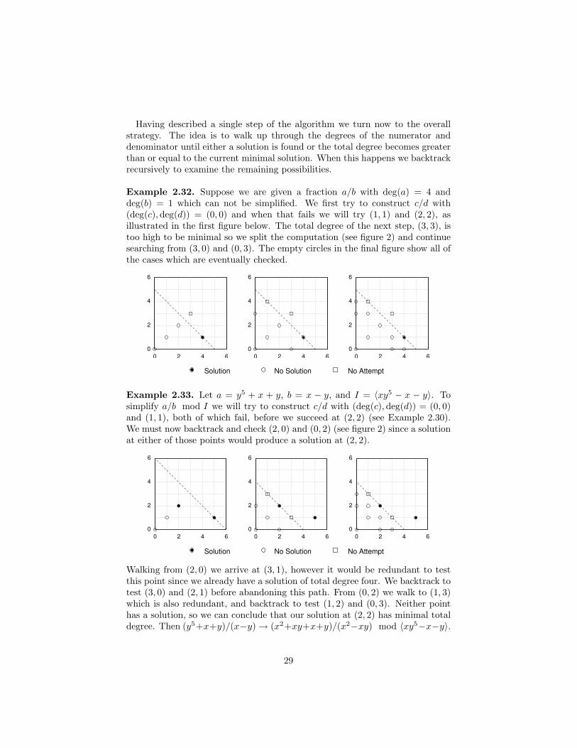
Having described a single step of the algorithm we turn now to the overallstrategy. The idea is to walk up through the degrees of the numerator anddenominator until either a solution is found or the total degree becomes greaterthan or equal to the current minimal solution. When this happens we backtrackrecursively to examine the remaining possibilities.
Example 2.32. Suppose we are given a fraction a/b with deg(a) = 4 anddeg(b) = 1 which can not be simplified. We first try to construct c/d with(deg(c),deg(d)) = (0, 0) and when that fails we will try (1, 1) and (2, 2), asillustrated in the first figure below. The total degree of the next step, (3, 3), istoo high to be minimal so we split the computation (see figure 2) and continuesearching from (3, 0) and (0, 3). The empty circles in the final figure show all ofthe cases which are eventually checked.
0 6420
2
4
6
����
0 6420
2
4
6
����
0 6420
2
4
6
����
Solution No Solution No Attempt
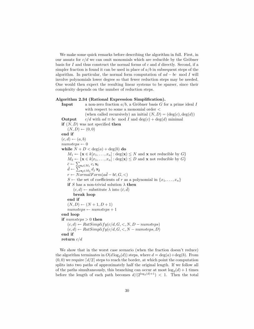
Example 2.33. Let a = y5 + x + y, b = x − y, and I = 〈xy5 − x − y〉. Tosimplify a/b mod I we will try to construct c/d with (deg(c),deg(d)) = (0, 0)and (1, 1), both of which fail, before we succeed at (2, 2) (see Example 2.30).We must now backtrack and check (2, 0) and (0, 2) (see figure 2) since a solutionat either of those points would produce a solution at (2, 2).
0 6420
2
4
6
0 6420
2
4
6
0 6420
2
4
6
����
Solution No Solution No Attempt
Walking from (2, 0) we arrive at (3, 1), however it would be redundant to testthis point since we already have a solution of total degree four. We backtrack totest (3, 0) and (2, 1) before abandoning this path. From (0, 2) we walk to (1, 3)which is also redundant, and backtrack to test (1, 2) and (0, 3). Neither pointhas a solution, so we can conclude that our solution at (2, 2) has minimal totaldegree. Then (y5+x+y)/(x−y)→ (x2+xy+x+y)/(x2−xy) mod 〈xy5−x−y〉.
29
We make some quick remarks before describing the algorithm in full. First, inour ansatz for c/d we can omit monomials which are reducible by the Grobnerbasis for I and thus construct the normal forms of c and d directly. Second, if asimpler fraction is found it can be used in place of a/b in subsequent steps of thealgorithm. In particular, the normal form computation of ad − bc mod I willinvolve polynomials lower degree so that fewer reduction steps may be needed.One would then expect the resulting linear systems to be sparser, since theircomplexity depends on the number of reduction steps.
Algorithm 2.34 (Rational Expression Simplification).Input a non-zero fraction a/b, a Grobner basis G for a prime ideal I
with respect to some a monomial order <(when called recursively) an initial (N,D) = (deg(c),deg(d))
Output c/d with ad ≡ bc mod I and deg(c) + deg(d) minimalif (N,D) was not specified then
(N,D)← (0, 0)end if(c, d)← (a, b)numsteps← 0while N + D < deg(a) + deg(b) do
M1 ← {x ∈ k[x1, . . . , xn] : deg(x) ≤ N and x not reducible by G}M2 ← {x ∈ k[x1, . . . , xn] : deg(x) ≤ D and x not reducible by G}c←
∑xi∈M1
ci xi
d←∑
xj∈M2dj xj
r ← NormalForm(ad− bc, G, <)S ← the set of coefficients of r as a polynomial in {x1, . . . , xn}if S has a non-trivial solution λ then
(c, d)← substitute λ into (c, d)break loop
end if(N,D)← (N + 1, D + 1)numsteps← numsteps + 1
end loopif numsteps > 0 then
(c, d)← RatSimplify(c/d, G,<,N, D − numsteps)(c, d)← RatSimplify(c/d, G,<,N − numsteps,D)
end ifreturn c/d
We show that in the worst case scenario (when the fraction doesn’t reduce)the algorithm terminates in O(d log2(d)) steps, where d = deg(a)+deg(b). From(0, 0) we require dd/2e steps to reach the border, at which point the computationsplits into two paths of approximately half the original length. If we follow allof the paths simultaneously, this branching can occur at most log2(d) + 1 timesbefore the length of each path becomes d/(2log2(d)+1) < 1. Then the total
30
number of steps is bounded by
log2(d)+2∑i=1
2i−1d/2i =d
2(log2(d) + 2) ∈ O(d log2(d))
Note however that the size of the linear systems can not be controlled. Ingeneral there are 1
n!
∏n−1i=0 (d+ i) monomials in n variables with degree less than
d, and potentially all of them can appear in each linear system along the border.When d is large relative to n this number is proportional to dn, so the methodbecomes impractical for problems of high degree. It is for precisely this reasonthat we start at (0, 0) and walk up, as opposed to some other approach. Inthe event that a/b simplifies to c/d, the size of the linear systems which weencounter will depend on deg(c) + deg(d) instead of deg(a) + deg(b).
31
Appendix A
Implementation
A.1 PolynomialIdeals in Maple 10
We have written a new Maple 10 package for ideal theoretic computationscalled PolynomialIdeals which we have used extensively to experiment withalgorithms and to develop examples for this thesis. We have implemented adata-structure for ideals of k[x1, . . . , xn], new routines for Grobner bases, andvarious ideal-theoretic operations, including all of the operations of Section 1.4.
In this section we introduce the package and show how it can be used toperform all of the computations in Chapter 1. In the later sections we use theseroutines to implement the algorithms of Chapter 2. To begin, we first load thepackage using Maple’s with command. This allows us to construct ideals usingan angled-bracket notation. The ideal J below is assumed to lie in the ringQ[x, y, z] by default.
> with(PolynomialIdeals):
Warning, the assigned name <, > now has a global binding
Warning, the protected name subset has been redefined and unprotected
> J := <x*y-z, x^2+z>;
J := 〈xy − z, x2 + z〉
Note that Maple reserves the capital letter I for the imaginary unit, so wewill use the letters J and K to represent ideals. To compute Grobner bases itis necessary understand how Maple represents monomial orders. They appearas functions of the ring variables given as an argument to the Grobner basiscommand. For example, lexicographic order with x > y > z is specified asplex(x, y, z) in Maple syntax below.
> PolynomialIdeals:-GroebnerBasis(J,plex(x,y,z));
[z2 + y2z, yz + xz, xy − z, x2 + z]
32
The other term orders are represented similarly: ’grlex’ is graded lexicographicorder and ’tdeg’ is graded reverse lexicographic order. Below we compute aGrobner basis for J using graded reverse lexicographic order with z > x > y.We first alias PolynomialIdeals:-GroebnerBasis to GroebnerBasis so that wedon’t have to type as much.
> GroebnerBasis := PolynomialIdeals:-GroebnerBasis: # alias
> GroebnerBasis(J,tdeg(z,x,y));
[xy − z, x2 + z, yz + xz, z2 + y2z]
The ’prod’ order constructs an elimination order as a product of monomialorders. In the computation below, we compare monomials first using gradedlexicographic order with x > y with ties broken by lexicographic order on z.
> GroebnerBasis(J,prod(grlex(x,y),plex(z)));
[yz + xz, z2 + y2z, xy − z, x2 + z]
Maple’s Grobner basis commands return the unique reduced Grobner basiswhich is primitive and fraction-free, sorted in the monomial order. We will usethe internal PolynomialIdeals command, since it implements new functionalitynot yet available in the standard command. For example, to run the extendedBuchberger algorithm we can use the following syntax.
> G, C := GroebnerBasis([x*y-z, x^2+z], tdeg(z,x,y), method=extended);
G, C := [xy − z, x2 + z, yz + xz, z2 + y2z], [[1, 0], [0, 1], [−x, y], [−xy − z, y2]]
The output is two lists, the first of which is the sorted reduced Grobner basis.The second list defines the rows of a transformation matrix whose dot productwith the vector of generators gives the Grobner basis, as shown below.
1 00 1−x y
−xy − z y2
[xy − zx2 + z
]=
xy − zx2 + zyz + xzz2 + y2z
To compute normal forms we will also use an internal command which can
compute a list of quotients (see Algorithm 1.13) and assign them to an optionalfourth argument. Below we compute f ÷G→ r and assign the quotients to Q.
> NormalForm := PolynomialIdeals:-NormalForm: # alias
> f := x^3-x*y^2+x*z+y*z;
f := x3 − xy2 + xz + yz> r := NormalForm(f, G, tdeg(z,x,y), ’Q’); Q;
r := 0[−y, x, 0, 0]
33
> ’f’ = Q[1]*G[1] + Q[2]*G[2] + ’r’; # don’t evaluate f and r
f = −y(xy − z) + x(x2 + z) + r> evalb(expand(%)); # evaluate and test the equation
true
The package implements all of the algorithms of Section 1.4. For example, tointersect the ideals of Example 1.28 one would type:
> Intersect(<x-1,y-1>, <x-1,y+1>);
〈x− 1, y2 − 1〉
The Quotient command computes ideal quotients. In Example 1.34 we com-puted 〈x2, y2 − 1〉 : 〈x, y − 1〉 as the intersection of 〈x2, y2 − 1〉 : 〈x〉 and〈x2, y2 − 1〉 : 〈y − 1〉. We can do this in Maple as follows.
> Q1 := Quotient(<x^2, y^2-1>, x);
Q1 := 〈x, y2 − 1〉> Q2 := Quotient(<x^2, y^2-1>, y-1);
Q1 := 〈y + 1, x2〉> Intersect(Q1,Q2);
〈x2, xy + x, y2 − 1〉
Of course, the Quotient command can also perform these steps automatically.
> Quotient(<x^2, y^2-1>, <x,y-1>);
〈x2, xy + x, y2 − 1〉
To compute Grobner bases for modules we will employ a useful trick. Considerthe module from Example 1.57 whose generators are given below. We willcompute a Grobner basis for this module using position over term graded-reverselexicographic order with x > y.
M =⟨[
y2 − x0
],
[x2 − xy
0
],
[0
y2 − x
],
[0
x2 − xy
],
[y1
]⟩The trick is to introduce dummy variables for each module position, such as{e1, e2, . . . }, and the polynomials eiej = 0 for all i 6= j. The dummy variablesprevent the different components from interacting, while eiej = 0 ensures thatS(f, g) = 0 if f and g have leading monomials in distinct components.
> M := [[(y^2-x),0], [(x^2-x*y),0], [0,(y^2-x)], [0,(x^2-x*y)], [y,1]];
M := [[(y2 − x), 0], [(x2 − xy), 0], [0, (y2 − x)], [0, (x2 − xy)], [y, 1]]> J := <e[1]*e[2], map(inner, M, [e[1],e[2]])>;
J := 〈e1e2, (y2 − x)e1, (x2 − xy)e1, (y2 − x)e2, (x2 − xy)e2, ye1 + e2〉
34
Next we compute the Grobner basis for this ideal. We can emulate TOP orPOT using a product order, placing the original variables first or last, respec-tively. It does not matter what order is chosen for the dummy variables.
> G := GroebnerBasis(J, prod(plex(e[1],e[2]), tdeg(x,y))); # POT order
G := [e2y2 − e2x, e2xy − e2x, e2x
2 − e2x, ye1 + e2, e1x + ye2, e22, e1e2]
Finally we discard polynomials which are not linear in the ei. The result isa Grobner basis for the module, which we will convert into vector form. Thebasis differs with that of Example 1.57 only because it has been reduced.
> G := remove(a -> degree(a, {e[1],e[2]}) > 1, G);
G := [e2y2 − e2x, e2xy − e2x, e2x
2 − e2x, ye1 + e2, e1x + ye2]> GV := map(a->map2(coeff, a, [e[1],e[2]]), G);
GV := [[0, y2 − x], [0, xy − x], [0, x2 − x], [y, 1], [x, y]]> map(Vector, GV);[[
0y2 − x
],
[0
xy − x
],
[0
x2 − x
],
[y1
],
[xy
]]We write a short Maple program to perform these steps automatically. It
takes as arguments a list of module elements, a monomial order, and either’TOP’ or ’POT’ for term over position or position over term order, respectively.
ModuleGB := proc(M::list(list), tord, ordertype)
local N, e, i, j, V, J, G, mtord;
N := nops(M[1]);
V := [seq(e[i], i=1..N)];
J := [op(map(inner, M, V)), seq(seq(e[i]*e[j], j=1..i-1), i=2..N)];
if ordertype=’POT’ then
mtord := ’prod’(’plex’(op(V)), tord);
else
mtord := ’prod’(tord, ’plex’(op(V)));
end if;
G := GroebnerBasis(J, mtord);
G := remove(a->degree(a,{op(V)}) > 1, G);
G := map(a->map2(coeff, a, V), G);
end proc:
We test the command on the previous example.
> ModuleGB(M, tdeg(x,y), POT);
[[0, y2 − x], [0, xy − x], [0, x2 − x], [y, 1], [x, y]]
35
This computation comes from Example 2.20. We compute a Grobner basisusing term over position graded lexicographic order with x > y.
> M := [[x-y, y^5+x+y], [y^5-2, -y^9-y^5+y^4], [0, x y^5-x-y]]:
> map(Vector,M);[[x− y
y5 + x + y
],
[y5 − 2
−y9 − y5 + y4
],
[0
xy5 − x− y
]]> G := ModuleGB(M, grlex(x,y), TOP):
> map(Vector, G);[[x2 − xy
x + y + x2 + xy
],
[x− y
y5 + x + y
],
[xy4 − 2xy4 + y4
]]
A.2 Inverses and Exact Division
Recall from Section 2.1 how we can compute inverses in k[x1, . . . , xn]/I usingthe extended Buchberger algorithm. Given f ∈ k[x1, . . . , xn]/I, we compute aGrobner basis G for 〈f, I〉 using any monomial order. If 1 ∈ G then f is invert-ible, and we can write 1 as a multiple of f modulo I. We demonstrate usingf = x and I = 〈x2 + y, y2 + 1〉 from Example 2.2. The Generators command isused to get the set of generators for the ideal.
> f := x;
f := x> J := <x^2+y, y^2+1>;
J := 〈x2 + y, y2 + 1〉> F := [f, op(Generators(J))];
F := [x, x2 + y, y2 + 1]> G, C := GroebnerBasis(F, grlex(x,y), method=extended);
G, C := [1], [[xy, 1,−y]]> finv := C[1][1];
finv := xy> NormalForm(f*finv, J, grlex(x,y)); # check
1
The general case of polynomial division is not much more complicated. Letf = xy3 + x + 1 and I = 〈xy5 − x − y〉 from Example 2.8. We divideg = xy3+y3+xy+y2 by f modulo I using graded lexicographic order with x > y.
> f := x*y^3+x+1;
f := xy3 + x + 1> g := x*y^3+y^3+x*y+y^2
g := xy3 + y3 + xy + y2
36
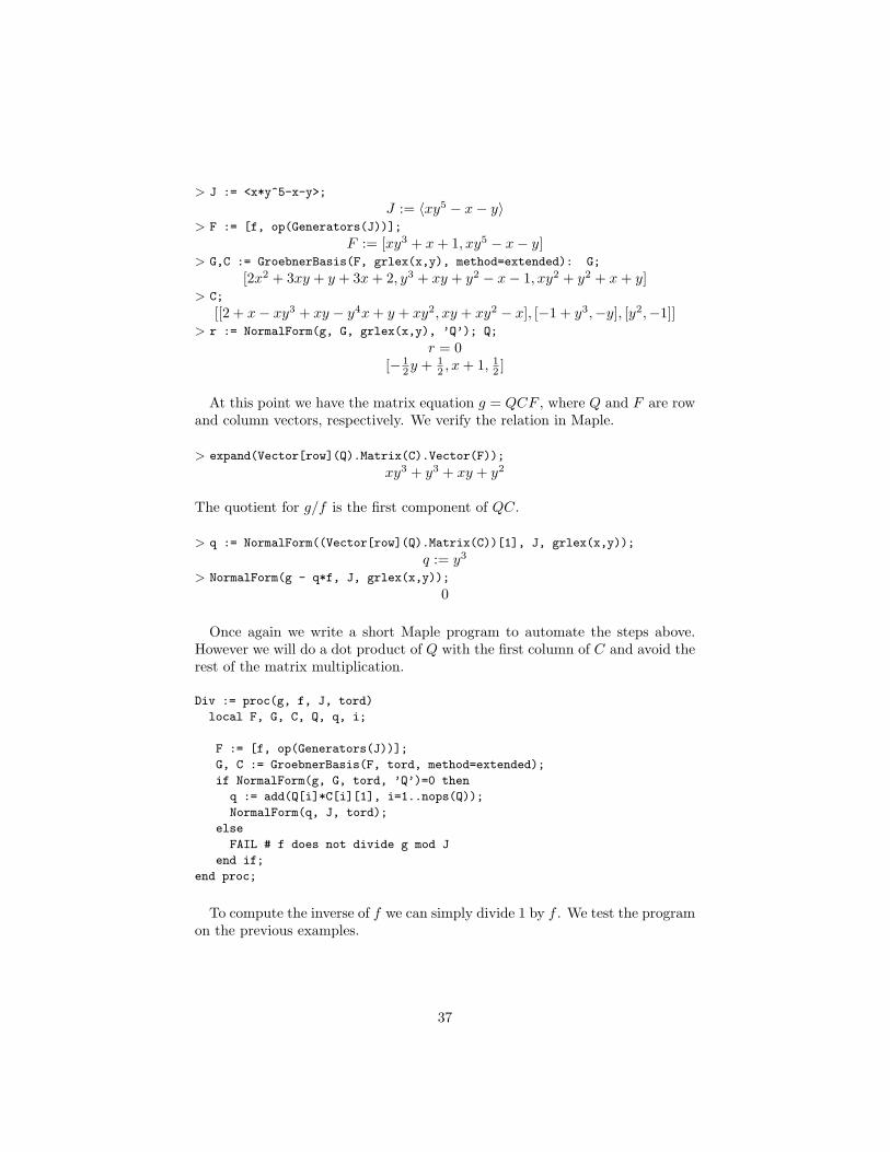
> J := <x*y^5-x-y>;
J := 〈xy5 − x− y〉> F := [f, op(Generators(J))];
F := [xy3 + x + 1, xy5 − x− y]> G,C := GroebnerBasis(F, grlex(x,y), method=extended): G;
[2x2 + 3xy + y + 3x + 2, y3 + xy + y2 − x− 1, xy2 + y2 + x + y]> C;
[[2 + x− xy3 + xy − y4x + y + xy2, xy + xy2 − x], [−1 + y3,−y], [y2,−1]]> r := NormalForm(g, G, grlex(x,y), ’Q’); Q;
r = 0[− 1
2y + 12 , x + 1, 1
2 ]
At this point we have the matrix equation g = QCF , where Q and F are rowand column vectors, respectively. We verify the relation in Maple.
> expand(Vector[row](Q).Matrix(C).Vector(F));
xy3 + y3 + xy + y2
The quotient for g/f is the first component of QC.
> q := NormalForm((Vector[row](Q).Matrix(C))[1], J, grlex(x,y));
q := y3
> NormalForm(g - q*f, J, grlex(x,y));
0
Once again we write a short Maple program to automate the steps above.However we will do a dot product of Q with the first column of C and avoid therest of the matrix multiplication.
Div := proc(g, f, J, tord)
local F, G, C, Q, q, i;
F := [f, op(Generators(J))];
G, C := GroebnerBasis(F, tord, method=extended);
if NormalForm(g, G, tord, ’Q’)=0 then
q := add(Q[i]*C[i][1], i=1..nops(Q));
NormalForm(q, J, tord);
else
FAIL # f does not divide g mod J
end if;
end proc;
To compute the inverse of f we can simply divide 1 by f . We test the programon the previous examples.
37
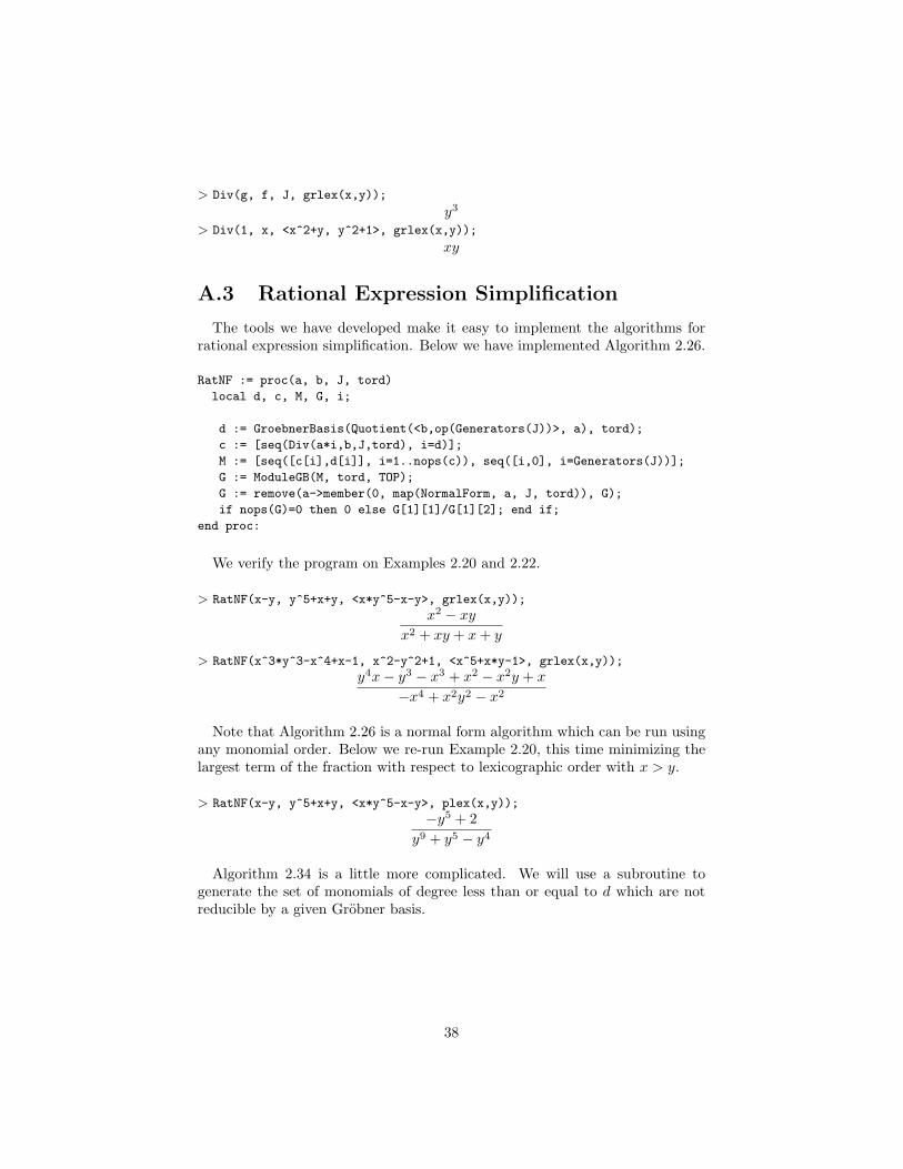
> Div(g, f, J, grlex(x,y));
y3
> Div(1, x, <x^2+y, y^2+1>, grlex(x,y));
xy
A.3 Rational Expression Simplification
The tools we have developed make it easy to implement the algorithms forrational expression simplification. Below we have implemented Algorithm 2.26.
RatNF := proc(a, b, J, tord)
local d, c, M, G, i;
d := GroebnerBasis(Quotient(<b,op(Generators(J))>, a), tord);
c := [seq(Div(a*i,b,J,tord), i=d)];
M := [seq([c[i],d[i]], i=1..nops(c)), seq([i,0], i=Generators(J))];
G := ModuleGB(M, tord, TOP);
G := remove(a->member(0, map(NormalForm, a, J, tord)), G);
if nops(G)=0 then 0 else G[1][1]/G[1][2]; end if;
end proc:
We verify the program on Examples 2.20 and 2.22.
> RatNF(x-y, y^5+x+y, <x*y^5-x-y>, grlex(x,y));
x2 − xy
x2 + xy + x + y
> RatNF(x^3*y^3-x^4+x-1, x^2-y^2+1, <x^5+x*y-1>, grlex(x,y));
y4x− y3 − x3 + x2 − x2y + x
−x4 + x2y2 − x2
Note that Algorithm 2.26 is a normal form algorithm which can be run usingany monomial order. Below we re-run Example 2.20, this time minimizing thelargest term of the fraction with respect to lexicographic order with x > y.
> RatNF(x-y, y^5+x+y, <x*y^5-x-y>, plex(x,y));
−y5 + 2y9 + y5 − y4
Algorithm 2.34 is a little more complicated. We will use a subroutine togenerate the set of monomials of degree less than or equal to d which are notreducible by a given Grobner basis.
38
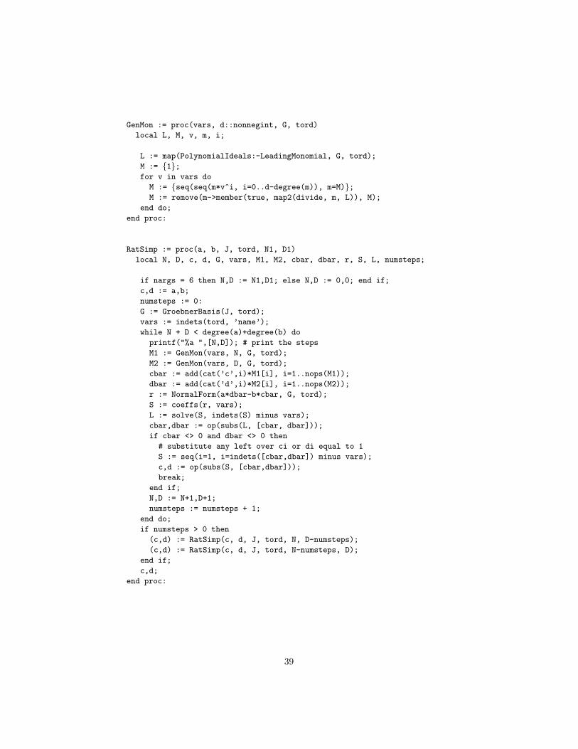
GenMon := proc(vars, d::nonnegint, G, tord)
local L, M, v, m, i;
L := map(PolynomialIdeals:-LeadingMonomial, G, tord);
M := {1};for v in vars do
M := {seq(seq(m*v^i, i=0..d-degree(m)), m=M)};M := remove(m->member(true, map2(divide, m, L)), M);
end do;
end proc:
RatSimp := proc(a, b, J, tord, N1, D1)
local N, D, c, d, G, vars, M1, M2, cbar, dbar, r, S, L, numsteps;
if nargs = 6 then N,D := N1,D1; else N,D := 0,0; end if;
c,d := a,b;
numsteps := 0:
G := GroebnerBasis(J, tord);
vars := indets(tord, ’name’);
while N + D < degree(a)+degree(b) do
printf("%a ",[N,D]); # print the steps
M1 := GenMon(vars, N, G, tord);
M2 := GenMon(vars, D, G, tord);
cbar := add(cat(’c’,i)*M1[i], i=1..nops(M1));
dbar := add(cat(’d’,i)*M2[i], i=1..nops(M2));
r := NormalForm(a*dbar-b*cbar, G, tord);
S := coeffs(r, vars);
L := solve(S, indets(S) minus vars);
cbar,dbar := op(subs(L, [cbar, dbar]));
if cbar <> 0 and dbar <> 0 then
# substitute any left over ci or di equal to 1
S := seq(i=1, i=indets([cbar,dbar]) minus vars);
c,d := op(subs(S, [cbar,dbar]));
break;
end if;
N,D := N+1,D+1;
numsteps := numsteps + 1;
end do;
if numsteps > 0 then
(c,d) := RatSimp(c, d, J, tord, N, D-numsteps);
(c,d) := RatSimp(c, d, J, tord, N-numsteps, D);
end if;
c,d;
end proc:
39
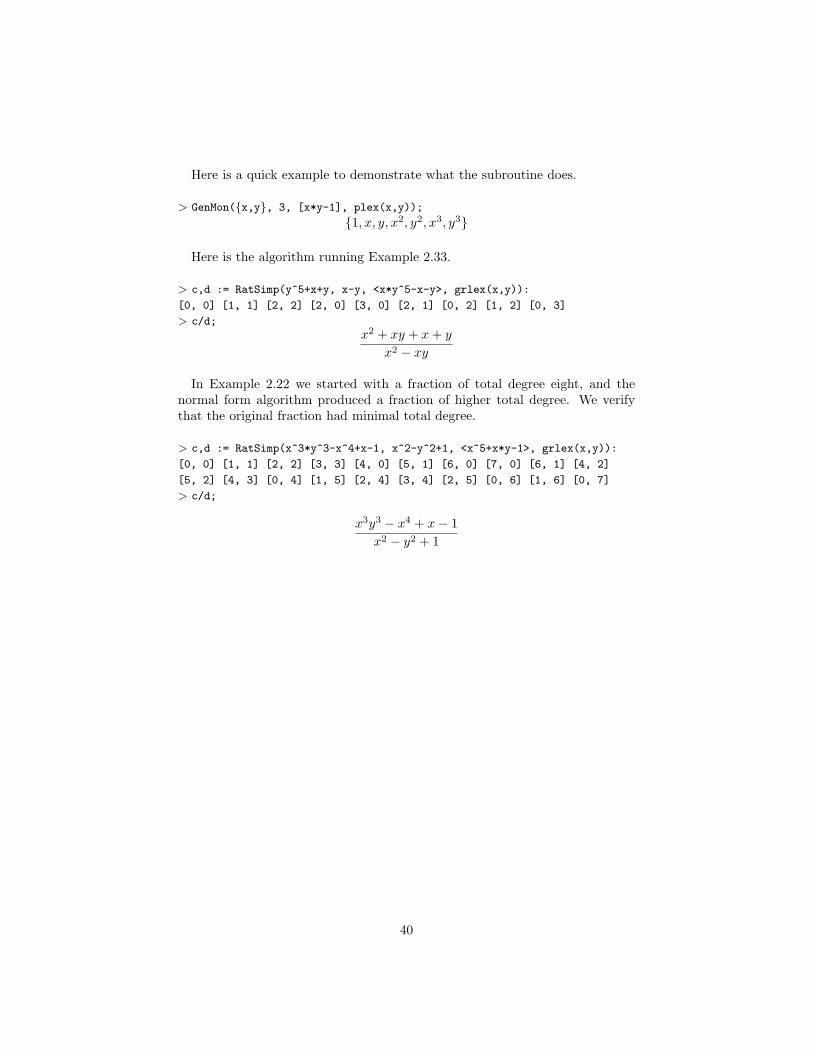
Here is a quick example to demonstrate what the subroutine does.
> GenMon({x,y}, 3, [x*y-1], plex(x,y));
{1, x, y, x2, y2, x3, y3}
Here is the algorithm running Example 2.33.
> c,d := RatSimp(y^5+x+y, x-y, <x*y^5-x-y>, grlex(x,y)):
[0, 0] [1, 1] [2, 2] [2, 0] [3, 0] [2, 1] [0, 2] [1, 2] [0, 3]
> c/d;x2 + xy + x + y
x2 − xy
In Example 2.22 we started with a fraction of total degree eight, and thenormal form algorithm produced a fraction of higher total degree. We verifythat the original fraction had minimal total degree.
> c,d := RatSimp(x^3*y^3-x^4+x-1, x^2-y^2+1, <x^5+x*y-1>, grlex(x,y)):
[0, 0] [1, 1] [2, 2] [3, 3] [4, 0] [5, 1] [6, 0] [7, 0] [6, 1] [4, 2]
[5, 2] [4, 3] [0, 4] [1, 5] [2, 4] [3, 4] [2, 5] [0, 6] [1, 6] [0, 7]
> c/d;
x3y3 − x4 + x− 1x2 − y2 + 1
40
Bibliography
[AL94] W. Adams, P. Loustaunau. An Introduction to Grobner Bases. AMS,Providence, 1994.
[Buc79] B. Buchberger. A criterion for detecting unnecessary reductions in theconstruction of Grobner bases. Lecture Notes in Computer Science, 72, pp.3-21, 1979.
[Buc85] B. Buchberger. Grobner Bases: An algorithmic method in polynomialideal theory. in Multidimensional systems theory, pp. 184-232, Reidel, 1985.
[BW93] T. Becker, V. Weispfenning. Grobner Bases : A Computational Ap-proach to Commutative Algebra. Springer-Verlag, New York Berlin Heidel-berg, 1993.
[CT98] M. Caboara, C. Traverso. Efficient Algorithms for Ideal Operations (Ex-tended Abstract). ISSAC 1998 Proceedings, pp. 147-152, 1998.
[Cox96] D. Cox, J. Little, D. O’Shea. Ideals, Varieties, and Algorithms. SecondEdition. Springer-Verlag, New York Berlin Heidelberg, 1996.
[Cox98] D. Cox, J. Little, D. O’Shea. Using Algebraic Geometry. Springer-Verlag, New York Berlin Heidelberg, 1998.
[Fau99] J.C. Faugere. A New Efficient Algorithm for Computing Grobner Bases(F4). Journal of Pure and Applied Algebra, 139, 1-3, pp. 61-88, 1999.
[Fau02] J.C. Faugere. A New Efficient Algorithm for Computing Grobner BasesWithout Reduction to Zero (F5). ISSAC 2002 Proceedings, pp. 75-83, 2002.
[Geb88] R. Gebauer, H. Moller. On an installation of Buchberger’s algorithm.Journal of Symbolic Computation, 6, pp. 275-286, 1988.
[Fro97] R. Froberg. An Introduction to Grobner Bases. Wiley & Sons, WestSussex, 1997.
[Mul01] J. Mulholland, M. Monagan. Algorithms for Trigonometric Polynomi-als. ISSAC 2001 Proceedings, pp. 245-252, 2001.
41