Rational Pessimism: Predicting Equity Returns

using Tobin’s q and Price/Earnings Ratios MATTHEW HARNEY AND EDWARD TOWER *

MATTHEW HARNEY is with the Investment Banking Division at Solomon Smith Barney. He is a 2002 Magna Cum Laude graduate of Duke University with a BS degree in Economics. Matthew.Harney@duke.edu EDWARD TOWER is a professor of economics at Duke. After earning his Ph.D. from Harvard, he taught at Tufts, the University of Auckland, Simon Fraser University and Nanjing University. He has also consulted with USAID, the World Bank and the Harvard Institute for International Development. Tower@econ.duke.edu

The Journal of Investing (forthcoming) January 2, 2003

Abstract

In the spring of 2000, two books predicted a substantial fall in the S&P500 Index. Robert Shiller’s Irrational Exuberance found that, historically, a high price earnings ratio, with real earnings averaged over 10 years, accurately predicts a low real rate of return from investing in the S&P500 Index. Smithers and Wright’s Valuing Wall Street found that a high Tobin’s q for the non-financial equities in the S&P500 does the same. We discover that q beats all variants of the PE ratio for predicting real rates of return over alternative horizons. We also formalize the feedback mechanisms considered in both books.

JEL Classification: G12

* This paper was written while Harney was an undergraduate at Duke. Its contents do not reflect the views of

Salomon Smith Barney or Citigroup. We are grateful to Luke Bayer, Bill Bernstein, Jim Dean, Omer Gokcekus, Bill

Kaempfer, Martin Salm, Allan Sleeman and members of the Western Washington University Economics

Department Seminar for comments and to the Duke University Arts and Sciences Research Council for funding.

2

In the spring of 2000, two books predicted a substantial fall in the Standard and Poor’s

500 Composite Index (henceforth S&P500). Robert Shiller’s Irrational Exuberance, found that,

historically, a high Price/Earnings ratio, with real earnings averaged over 10 years, predicts a low

real rate of return from investing in the S&P500. Andrew Smithers and Stephen Wright’s

Valuing Wall Street found that a high Tobin’s q for the non-financial equities in the S&P500 also

predicts a low real rate of return for this index. These pessimistic views, in sharp contrast with

more popular sanguine perceptions regarding recent equity valuations, motivated the criticism of

those most adherently attached to such optimism, such as Jonathan Laing (2000) and Gene

Epstein. Epstein, Barron’s economics editor, was particularly optimistic. His evaluation of

both books in several pieces in Barron’s was extremely critical. Epstein (May 8, 2000)

characterizes Robert Shiller’s use of trailing ten-year earnings averages in calculating

Price/Earnings ratios, as opposed to using only earnings from the current year, as a “bizarre

approach” that makes the stock market appear overvalued. He also expresses his distaste for the

Shiller calculation, and his preference for what he calls the “Shiller lite” P/E ratio, defined as the

ratio of price to the five-year trailing average of earnings. He declares his most preferred

alternative to be the “P/E Classic (four quarter trailing earnings).”

Epstein’s criticism of Smithers and Wright’s Valuing Wall Street also demonstrates an

attachment to buoyant “new economy” theories. By prioritizing the importance of intangible

assets in this “new era”, Epstein dismisses the insights Smithers and Wright’s research provides

regarding the overall valuation of the stock market, inclusive of those companies with a

substantial degree of intangible assets. Epstein (May 15, 2002) also considers the lack of an

explicit endorsement of Smithers and Wright’s approach by James Tobin, who devised the q

ratio in 1969 to predict changes in capital investment via signals from equity valuations, to be a

critical weakness. Epstein’s view of intellectual ownership, however, ignores the merits of using

the ideas of others for an originally unintended purpose to develop other compelling ideas, as

Smithers and Wright do. For Epstein, these perceived failings invalidate the research of Shiller,

and Smithers and Wright.

Epstein, however, fails to specify which approach is less faulty. We feel compelled to

evaluate his claims, and assess whether either book added value to our ability to predict the stock

market, and if there is some value added, which book added more of it.

3

Specifically, (1) we test both approaches against using the simple ratio of price to current

earnings (P/E1) to predict real rates of return; (2) we experiment with different lengths for the

trailing averages for earnings; (3) we use the alternative approaches to predict the real rate of

return for the S&P500 index over several different horizons and (4) we incorporate a feedback

mechanism, exploring whether a high real rate of return from the stock market in the past makes

investors more optimistic and boosts future returns.

INTUITION

Shiller’s Irrational Exuberance uses Price/Earnings ratios (henceforth PEs) to evaluate

equity valuations and corresponding investment returns over an extended historical horizon.

Stock prices should demonstrate a fundamental relationship with the ability of firms to generate

profits, expressed in the form of earnings. The magnitude of PEs should thus demonstrate

investors’ valuations of company profits. The existence of a fundamental relationship between

equity valuations and corporate profits, however, constrains the degree to which PEs can

rationally fluctuate, so these ratios should revert to their means. Sufficiently low PEs reflect an

overall undervaluation of the stock market; conversely, sufficiently high PEs suggest investors

overvalue the ability of firms to generate profits. Consequently, above average investment

returns should follow periods exhibiting relatively low PEs and below average investment

returns should follow periods with comparatively high PEs.

Although less popular than PEs, Smithers and Wright’s (2000, p.11) q ratio provides

similar insights regarding the valuation of the overall stock market. This ratio is expressed in the

following form:

.WorthNetCorporateMarketStockofValueq = (1)

In this formula, corporate net worth is the replacement cost of physical assets plus

financial assets minus liabilities. Accordingly, a q that exceeds one implies investors value

corporations at a level exceeding the value of underlying capital assets; a q less than one suggests

the opposite. A fundamental relationship should exist between stock market valuations and

underlying corporate assets; more simply, firms in the long run should be valued at their current

cost of creation and thus q should theoretically hover around one under rational expectations.1

Robertson and Wright (1998) demonstrate that q mean reverts through changes in stock market

4

values (the numerator) rather than through changes in corporate investment (the denominator) as

originally predicted by Tobin. Thus, above average investment returns should follow periods

exhibiting a below average q ratio and below average returns should follow periods with high q

ratios.

At year-end 2001, Shiller’s PE and Smithers and Wright’s q ratio significantly exceeded

the historical average of each measure of value. Thus, they both predicted investors would

experience poor returns over the intermediate term until these ratios approach more tenable

values.

DATA

Our research covers investment returns over the period year-end 1900 to year-end 2001.

This data set, however, includes data all the way back to 1871 due to the use of qs, which depend

on investment history, and 30-year trailing real earnings averages. Prices of the S&P are in real

terms using the January Consumer Price Index as the relevant deflator. Year-end figures are

used for the q ratio, dividends, and earnings. Shiller (2002) kindly provides the earnings,

dividends, and Consumer Price Index data. Wright alerted us to his (2002) article that

generously provides the q data used in this article.2

We use the December closing price of the S&P 500. This differs from Shiller, who uses

January averages, because Smithers and Wright’s qs are measured at year end, and all the

calculations in Valuing Wall Street pertain to calendar years. For the period 1900 to 1917, the

closing price was unavailable so we approximated it by the average value of the index in the

months of December and January.

We calculate real rates of return as annualized rates, assuming dividends are paid at the

end of the year, so the one-year rate of return is calculated as follows:

1t

tt

PPD1RoR

−

+= (2)

where Dt equals real dividends and Pt represents the real S&P 500 price at the end of year t.

RoRN denotes the real annualized geometric average rate of return over N years, assuming all

dividends are reinvested.3 Each rate of return was compared with the q and PEs at the beginning

of the period.

5

TESTING THE ALTERNATIVES

Should q or a PE be a better predictor on theoretical grounds? We would expect firms to

enter the industry whenever q is high, because that is when entering the industry is profitable.

This should drive down earnings, dividends and stock prices. Also, Siegel (2002, pp. 198-199)

points out that changes in the inflation rate alter the relationship between reported earnings and

the ideal measure of earnings. However, if the corporation income tax rises, we would expect a

given q to yield reduced earnings and dividends, and this should depress stock price. Suppose

that as economic development proceeds the cost of capital is driven down. We would expect q to

remain constant in the long run, but we would expect the earnings yield (1/PE) and the long run

rate of return on investment in the stock market to fall. Here PE out-predicts q. Earnings are

measured after corporation income tax, and in that regard PEs would also be expected to perform

better than q. But, they lack the mechanism whereby high q causes entry and on that ground

would be expected to work less well than q. Thus, it is not clear to us whether q or a PE would

be a better predictor a priori, which drives us to look at the data.

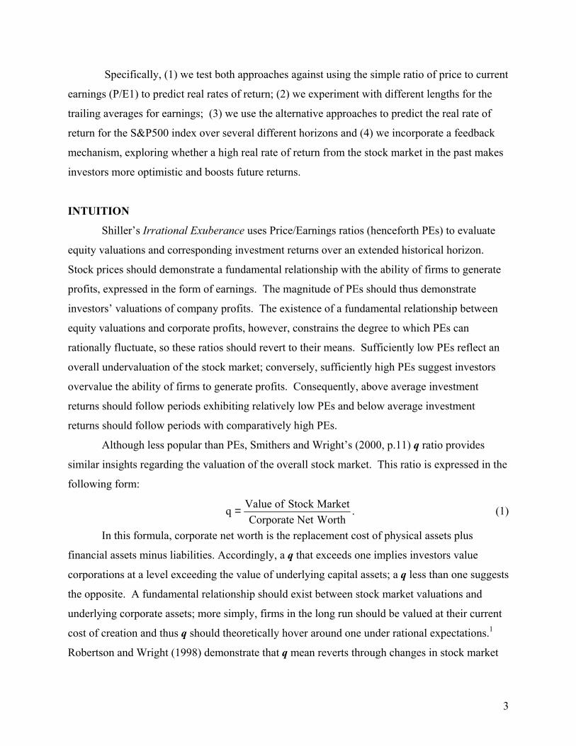
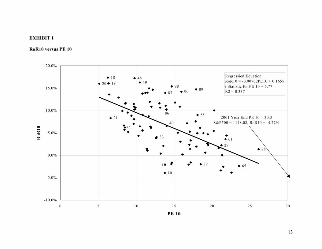
We wish to test the accuracy of alternative ways of predicting real rates of return. Our

notation defines PEN as the real price of the S&P500 index divided by the N-year trailing

average of real earnings for the S&P500 index. Our benchmark is Exhibit 1: RoR10 versus

PE10, which replicates the graph in Shiller (2000, p.11) for the period 1901-2001, using year-end

values instead of January averages for the PE10. Selected data points in our exhibits are labeled

with the last two digits of the year end for which q or PE10 is reported. Fitting a regression line

through the points on the graph shows the 10-year real rate of return to be a decreasing function

of PE10. The 2001 year-end PE10 is 30.3, and the regression line predicts a geometric average

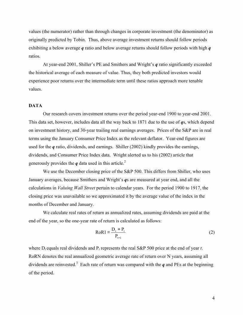
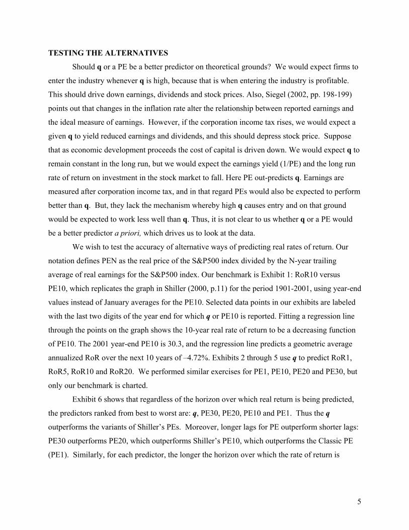
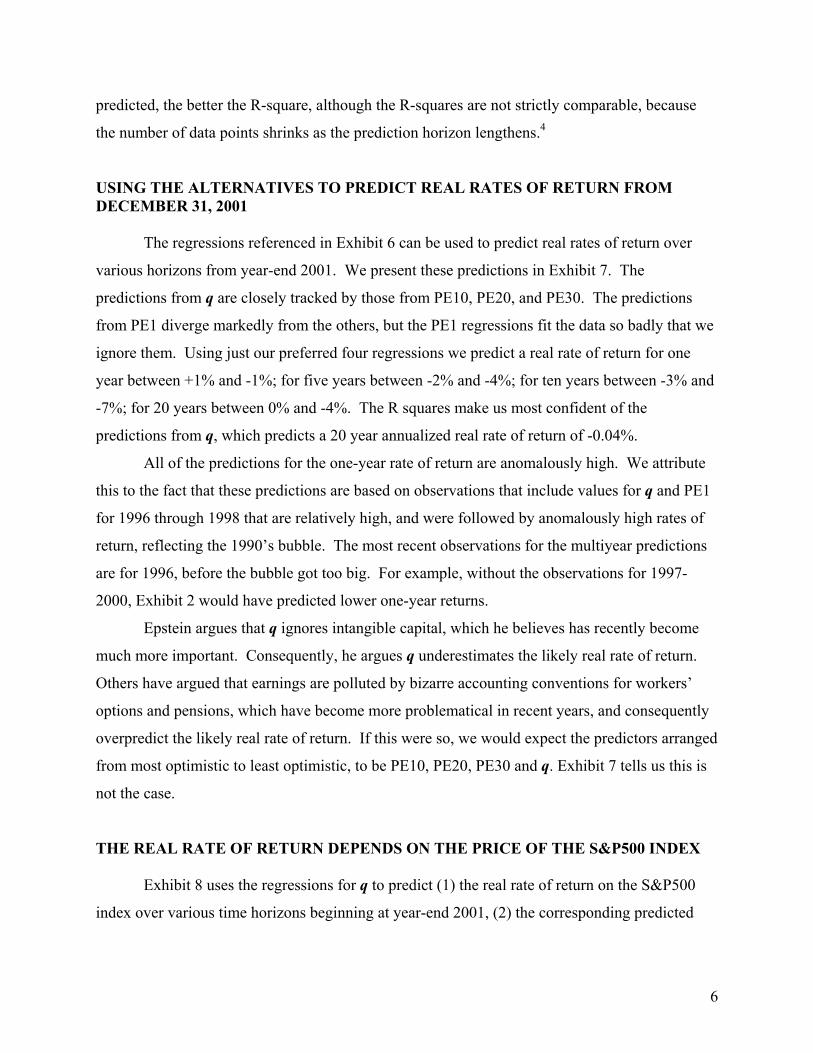
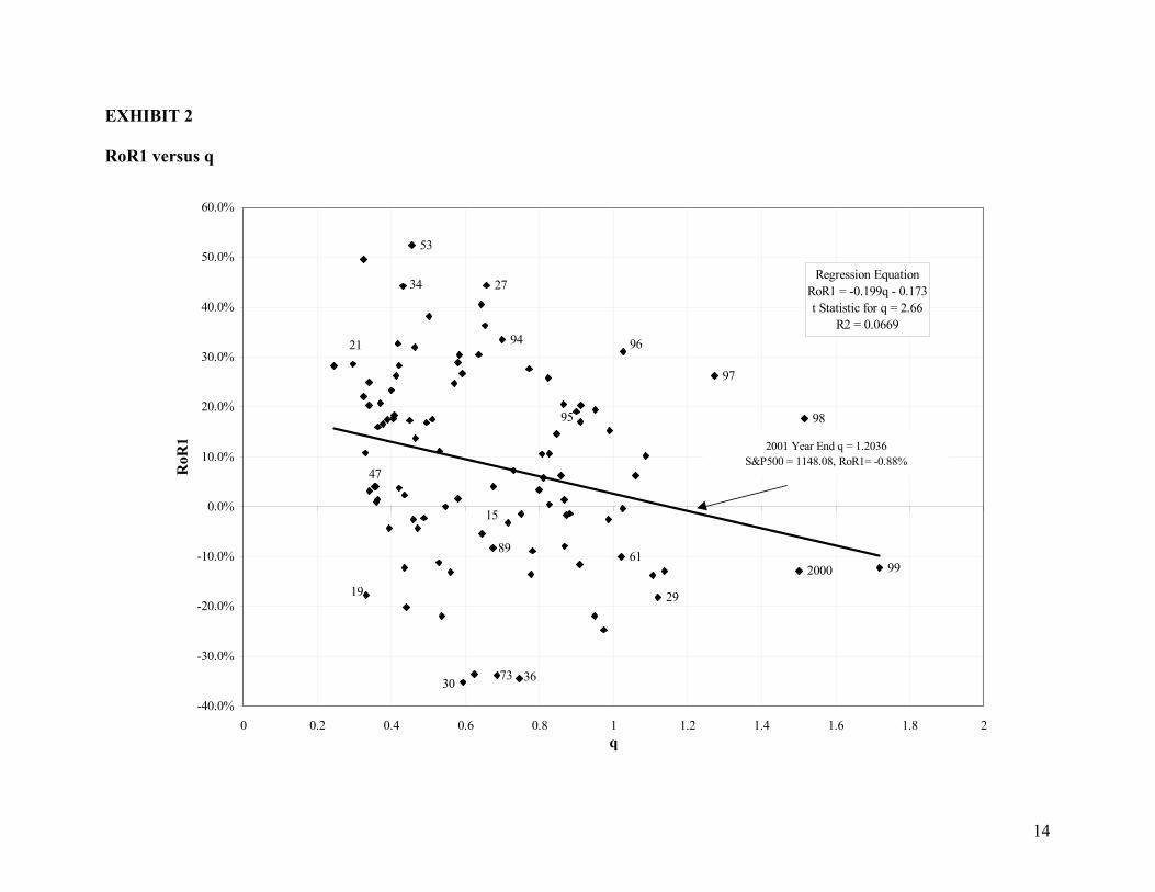
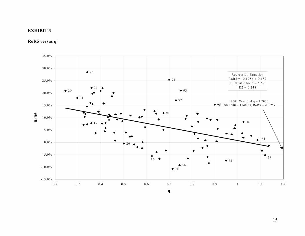
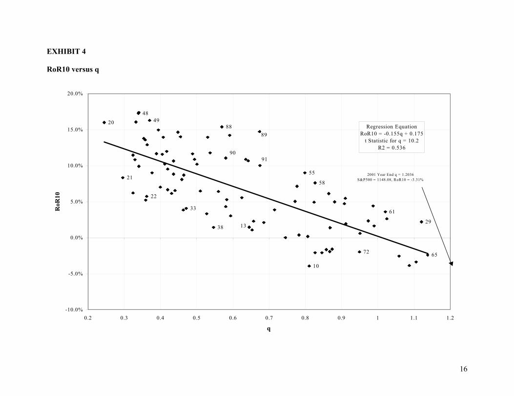
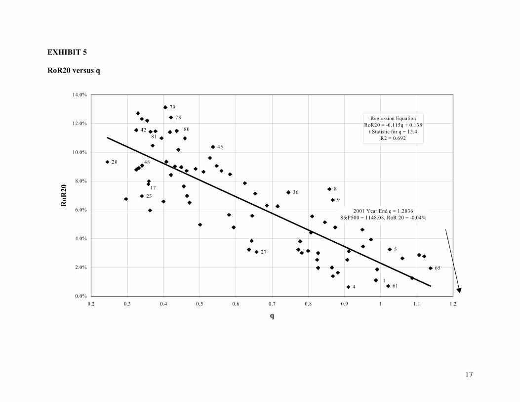
annualized RoR over the next 10 years of –4.72%. Exhibits 2 through 5 use q to predict RoR1,

RoR5, RoR10 and RoR20. We performed similar exercises for PE1, PE10, PE20 and PE30, but

only our benchmark is charted.

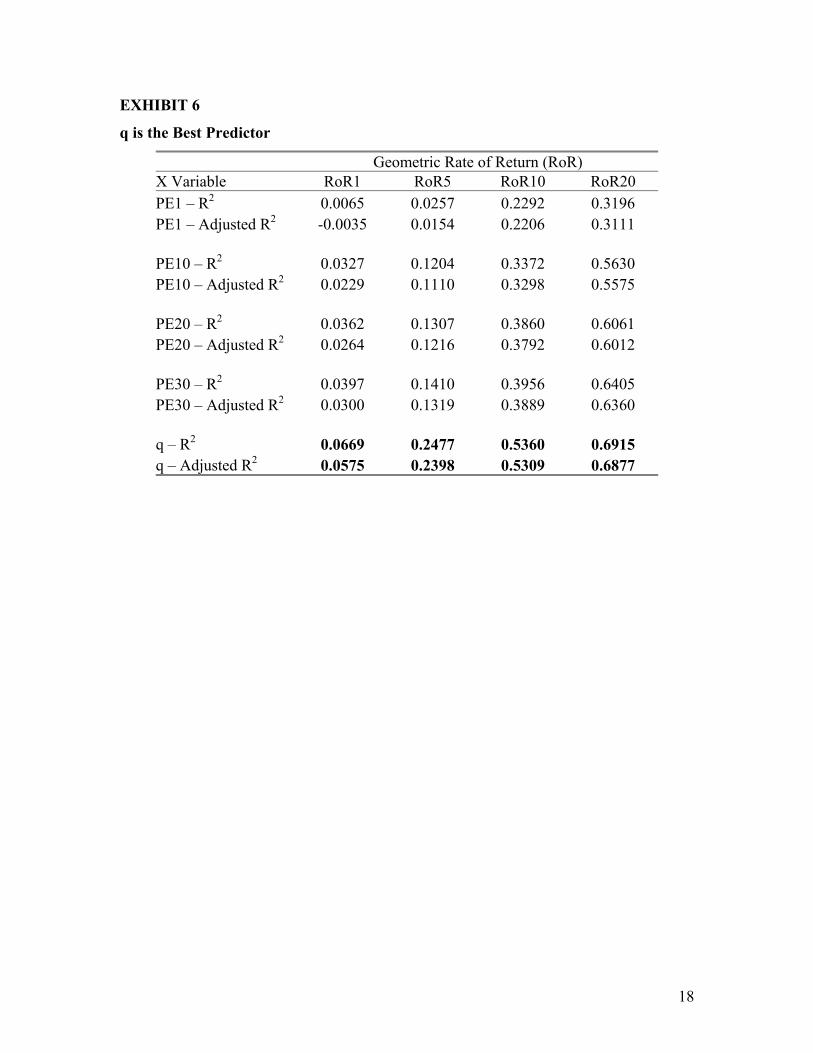
Exhibit 6 shows that regardless of the horizon over which real return is being predicted,

the predictors ranked from best to worst are: q, PE30, PE20, PE10 and PE1. Thus the q

outperforms the variants of Shiller’s PEs. Moreover, longer lags for PE outperform shorter lags:

PE30 outperforms PE20, which outperforms Shiller’s PE10, which outperforms the Classic PE

(PE1). Similarly, for each predictor, the longer the horizon over which the rate of return is

6

predicted, the better the R-square, although the R-squares are not strictly comparable, because

the number of data points shrinks as the prediction horizon lengthens.4

USING THE ALTERNATIVES TO PREDICT REAL RATES OF RETURN FROM DECEMBER 31, 2001

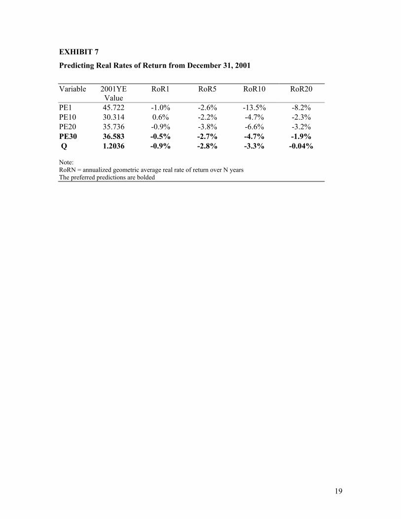
The regressions referenced in Exhibit 6 can be used to predict real rates of return over

various horizons from year-end 2001. We present these predictions in Exhibit 7. The

predictions from q are closely tracked by those from PE10, PE20, and PE30. The predictions

from PE1 diverge markedly from the others, but the PE1 regressions fit the data so badly that we

ignore them. Using just our preferred four regressions we predict a real rate of return for one

year between +1% and -1%; for five years between -2% and -4%; for ten years between -3% and

-7%; for 20 years between 0% and -4%. The R squares make us most confident of the

predictions from q, which predicts a 20 year annualized real rate of return of -0.04%.

All of the predictions for the one-year rate of return are anomalously high. We attribute

this to the fact that these predictions are based on observations that include values for q and PE1

for 1996 through 1998 that are relatively high, and were followed by anomalously high rates of

return, reflecting the 1990’s bubble. The most recent observations for the multiyear predictions

are for 1996, before the bubble got too big. For example, without the observations for 1997-

2000, Exhibit 2 would have predicted lower one-year returns.

Epstein argues that q ignores intangible capital, which he believes has recently become

much more important. Consequently, he argues q underestimates the likely real rate of return.

Others have argued that earnings are polluted by bizarre accounting conventions for workers’

options and pensions, which have become more problematical in recent years, and consequently

overpredict the likely real rate of return. If this were so, we would expect the predictors arranged

from most optimistic to least optimistic, to be PE10, PE20, PE30 and q. Exhibit 7 tells us this is

not the case.

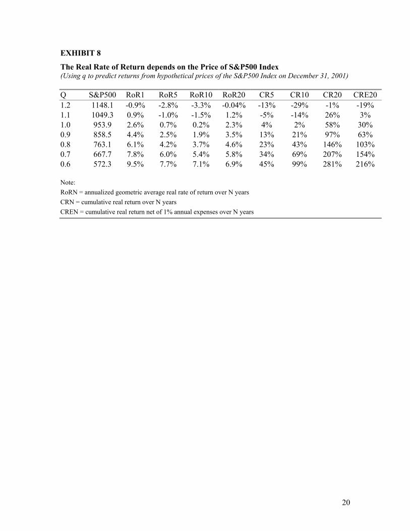
THE REAL RATE OF RETURN DEPENDS ON THE PRICE OF THE S&P500 INDEX

Exhibit 8 uses the regressions for q to predict (1) the real rate of return on the S&P500

index over various time horizons beginning at year-end 2001, (2) the corresponding predicted

7

cumulative real returns, and (3) the cumulative real returns over a 20 year horizon, assuming that

1% of the value of the investment is absorbed each year by mutual fund expenses.

The two leftmost columns of the top line of data show the actual value for q and the

S&P500 on year-end 2001. This line predicts a real rate of return of -0.9% over one year, of

-2.8% over 5 years, of -3.3% over 10 years, and of -0.04% over 20 years.

The subsequent lines perform the same exercise for alternative hypothetical prices for the

S&P500 on that date. In order to secure a 20-year real rate of return of +4.6% the S&P500

would have had to have fallen to 763, and even after falling to 572, the predicted real rate of

return is still less than +7%. These hypothetical rows enable us to predict the market going

forward. For example in July 2002, the S&P500 hit 858.48. At that time, we would have

predicted roughly a 1.9% real rate of return over the next 10 years. We say “roughly” because

this price was hit in July 2002 rather than at year-end 2001.

Based on data through year-end 2001, Exhibit 8 also predicts a cumulative real gain over

five years of -13%, over 10 years of -29%, and over 20 years of –1%. Note from the CR20

column, that the real return over 20 years is substantial only after the market falls significantly.

Finally, it is important for investors to be aware of how much high expense ratios eat into their

real rates of return. Consequently, in the last column, we present CRE 20, which depicts the

cumulative real return over 20 years, assuming that the investment advisor or mutual fund

charges one percent per year of the investment balance in expenses, well below the expense ratio

of many mutual funds. This turns our best estimate of the 20 year cumulative return from -1%

into -19%, and it shrinks our maximum cumulative return from +281% to the much more modest

+216%. It emphasizes the foolishness of investing in mutual funds or hiring investment advisors

who charge high expenses, without delivering comparably higher performance.

AMPLIFICATION AND THE FEEDBACK LOOP

Shiller (2000, p.44) discusses amplification mechanisms and feedback loops.

The amplification mechanisms work through a sort of feedback loop; later in this chapter they will also be described as a type of naturally occurring Ponzi process. Investors, their confidence and expectations buoyed by past price increases, bid up stock prices further, thereby enticing more investors to do the same, so that the cycle repeats again and again, resulting in an amplified response to the original precipitating factors. The feedback mechanism is widely mentioned in popular discourse as merely a hypothesis, often

8

regarded as unproven. In fact there is some evidence in support of such a feedback mechanism, as we shall see.

Shiller nicely fleshes out the microeconomics of these mechanisms. However, he leaves it

to us to include past performance in an equation which predicts future performance. This seems

to us, the most appropriate way to test Shiller’s idea, as it uses the data set on which his book is

based.

Smithers and Wright (2002, 121-123) make a similar point in a round about way. They

suggest that a strategy which dominates the others they consider is to hold stocks except “When

q Goes 50% Above Average, Hold Cash Until It goes Below Average.” Thus they suggest that

given q, shareholders garner better returns when the market has been rising recently and worse

returns when it has been falling. This only makes sense if past stock price momentum carries

forward. This is how we chose to model the process.

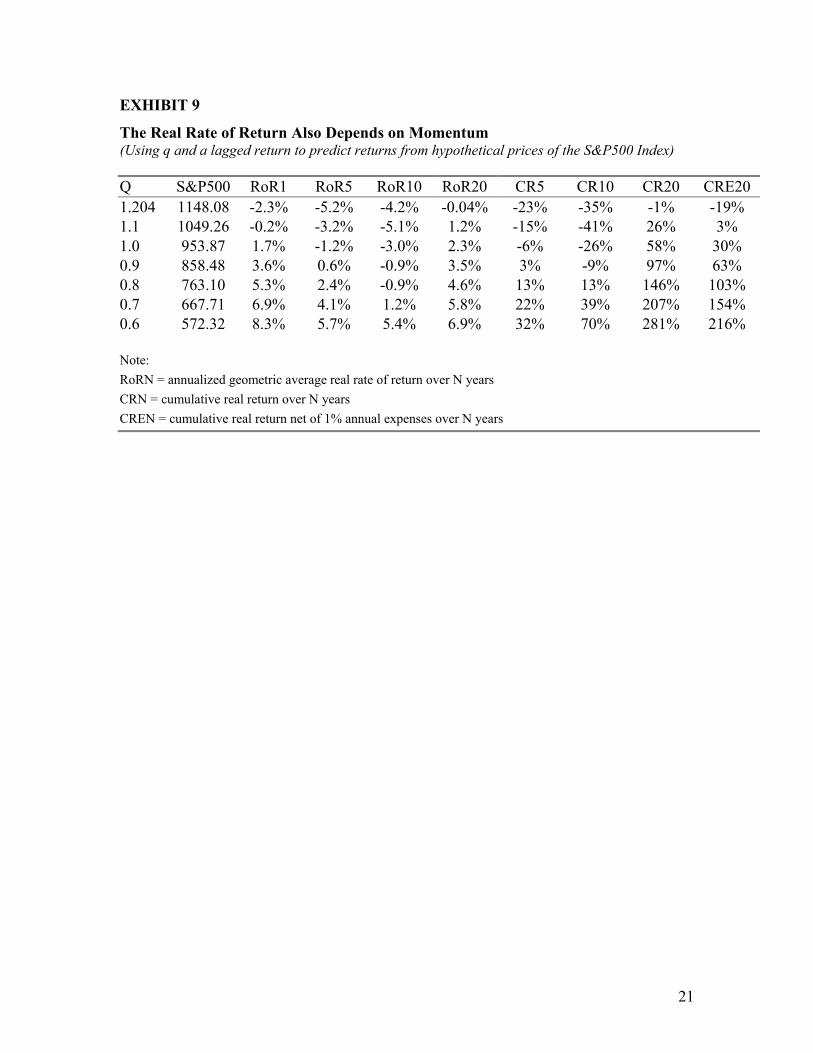
THE REAL RATE OF RETURN ALSO DEPENDS ON MOMENTUM

Exhibit 9 was created by using an equation to predict the rate of return from buying the

index and reinvesting the dividends over the following: a one year period, a 5 year period, a 10

year period, and a 20 year period. Exhibit 10 presents annual predictions. The prediction

equation is:

,c]RoRML[baqRoRN ++= (3)

where

RoRN is the annualized geometric rate of return over the next N years,

RoRML is the annualized geometric rate of return over the past M years, which we call

momentum;

a, b and c are constants.

We estimated the equation for various time lags, M, for the past rate of return and

selected the one with the highest R2 constraining b to be nonnegative. In each case, we find that a

is negative, which we expect as a high q means the market is overvalued. The M which gave the

best fit for each time period turned out in each case to be between 0 and 11 years, with the lag

generally declining as N increased.5. The estimated values for b were all positive, for the 1

through 17-year horizons. It was negative for the 18, 19 and 20 year horizons, so for predicting

those long-period returns we suppressed the momentum term. This means that when the returns

9

have been high in the market, investors are optimistic and keep putting money into the stock

market, pushing it up further, and increasing the future rate of return in the short run. Similarly,

if past returns are low, investors expect a lousy return in the future and the market continues to

tank. We believe the result for the 18, 19 and 20 year horizons reflects the idea that if at the start

of the period the market is trending downward, then reinvested dividends buy more shares,

which increases the predicted real rate of return over a sufficiently long time horizon. But we felt

these results might be anomalous, so we suppressed the momentum term in the results we present

for the 18, 19 and 20 year horizons. Note in Exhibit 9 that for the observed q, at year-end 2001,

the cumulative decline in the market is largest after 10 years.

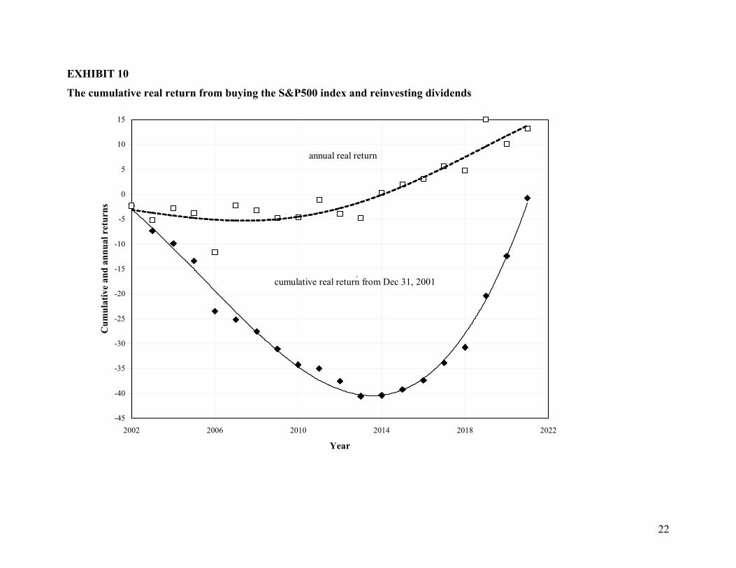
Exhibit 10 corresponds to the top line of data in Exhibit 9. It reflects the calculations that

predict the annualized rates of return from 1 through 20 years. From these we calculated

cumulative returns, which are marked with diamonds. The curves show the predictions

smoothed. The conclusion is that as of year-end 2001 we expected the real value of a portfolio

consisting of the S&P500 index with reinvested dividends to fall gradually until year-end 2013,

until ultimately it has fallen by 41 percent. Thus, an overvalued market takes a long time to reach

its nadir. After that the portfolio was expected to rebound through 2021. At that point, we expect

it will have almost recouped its value, being down by only 0.8%. The point here is that the

market falls slowly as the optimism is replaced by pessimism, due to low real returns. But then

fundamentals (a low q) push the market back up, and this makes investors more optimistic. The

squares show the predicted year by year percentage rates of real returns, constructed from the

diamonds. The line at the top of the graph shows the smoothed squares. It is the predicted annual

real rate of return graphed versus the year. Roughly speaking it is the derivative of the smoothed

cumulative returns curve, moving from –2.3 % for 2002 up to +13 % at year-end 2021.

Obviously, given this analysis, we did not expect the rapid fall of the S&P500 through October

2002.

HOW IMPORTANT IS THE FEEDBACK EFFECT?

Predicting the one year real rates of return from year-end 1900 through year-end 2000 (which

carries us through year-end 2001), with returns expressed as percent per year, and correcting for

first order correlation yields:

RoR1 = -28.6q + 0.972[RoR11L] + 21.0 (4)

10

(-3.35) (2.01) (4.48)

[.001] [.048] [.000]

where the t's are in parentheses and significance levels on a two-tailed test are in brackets. The

regression says that each one percentage point increase in the real rate of return over the last 11

years creates enough optimism among investors to raise the real rate of return over the

subsequent year by almost a full percent.

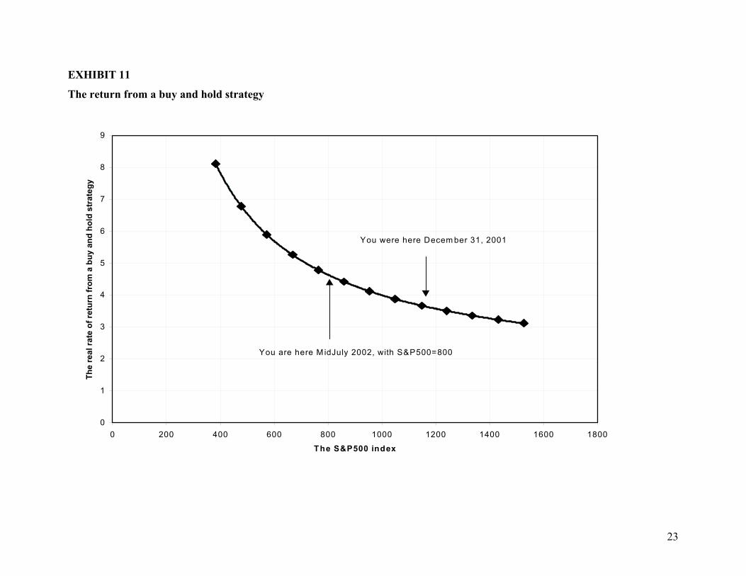
THE RETURN FROM A BUY AND HOLD STRATEGY FOR THE S&P500 INDEX

Now we predict the real rate of return from buying and holding the S&P500 index

forever, while consuming the dividends it pays. The rate of return from such a strategy is the

current dividend yield plus the rate of growth of dividends as Shiller (2000), and Smithers &

Wright (2000) discuss. Assuming the ratio of earnings to the capital stock stays constant, if the

ratio of dividends to the capital stock is also constant, then reinvestment as a fraction of the

capital stock should stay constant and the capital stock, earnings and dividends should continue

to grow as fast as they have done historically. Consequently, we postulate that firms maintain

the same ratio of dividends to the capital stock as they have on average since 1900. We call the

dividends which preserve this ratio, normalized dividends. This postulate implies that earnings

and dividends will continue to grow at the same rate as earnings have grown since 1900, 1.449

percent per year, and the real rate of return will equal this growth rate plus the normalized

dividend yield, where we define the normalized dividend yield as normalized dividends divided

by price.

Normalized dividends equal the average ratio of dividends to the capital stock, divided by

q, which is price/capital stock for the non-financial firms in the S&P500. Defining D as

dividends and P as the price of the S&P500, we calculate the average ratio of dividends to the

capital stock6 as the average of (D/P)q, since 1900, which is .02668.

This allows us to write the predicted real rate of return from buying and holding the S&P500

index as a function of the hypothetical values for q at year-end 2001, qH:

,q668.2449.1RBH

H

+= (5)

where RBH is expressed as a percent per year.

11

To express the return as a function of the hypothetical value for the S&P500 at year-end

2001, PH, we recognize that qH = (PH/ 1148.08)*1.204, where 1148.08 is the actual year-end

2001 value for the S&P500 and 1.204 is the actual value for q at year-end 2001. This yields an

alternative predictor:

.P544.2449.1RBH

H

+= (6)

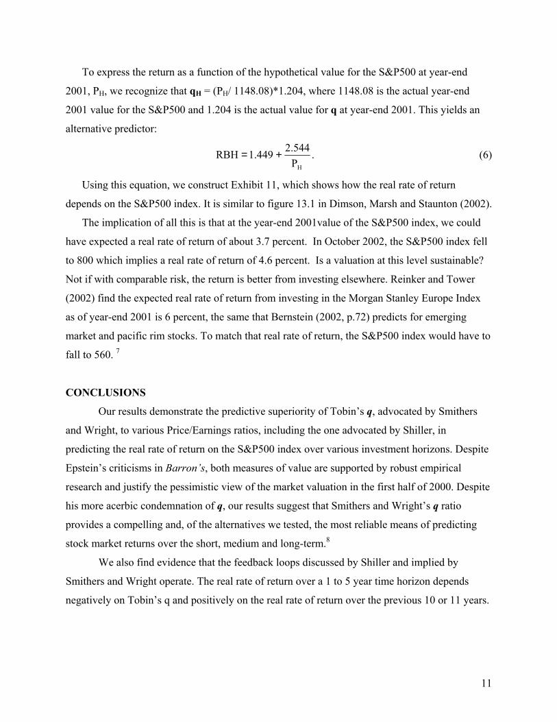
Using this equation, we construct Exhibit 11, which shows how the real rate of return

depends on the S&P500 index. It is similar to figure 13.1 in Dimson, Marsh and Staunton (2002).

The implication of all this is that at the year-end 2001value of the S&P500 index, we could

have expected a real rate of return of about 3.7 percent. In October 2002, the S&P500 index fell

to 800 which implies a real rate of return of 4.6 percent. Is a valuation at this level sustainable?

Not if with comparable risk, the return is better from investing elsewhere. Reinker and Tower

(2002) find the expected real rate of return from investing in the Morgan Stanley Europe Index

as of year-end 2001 is 6 percent, the same that Bernstein (2002, p.72) predicts for emerging

market and pacific rim stocks. To match that real rate of return, the S&P500 index would have to

fall to 560. 7

CONCLUSIONS

Our results demonstrate the predictive superiority of Tobin’s q, advocated by Smithers

and Wright, to various Price/Earnings ratios, including the one advocated by Shiller, in

predicting the real rate of return on the S&P500 index over various investment horizons. Despite

Epstein’s criticisms in Barron’s, both measures of value are supported by robust empirical

research and justify the pessimistic view of the market valuation in the first half of 2000. Despite

his more acerbic condemnation of q, our results suggest that Smithers and Wright’s q ratio

provides a compelling and, of the alternatives we tested, the most reliable means of predicting

stock market returns over the short, medium and long-term.8

We also find evidence that the feedback loops discussed by Shiller and implied by

Smithers and Wright operate. The real rate of return over a 1 to 5 year time horizon depends

negatively on Tobin’s q and positively on the real rate of return over the previous 10 or 11 years.

12

REFERENCES

Bernstein, William. The Four Pillars of Investing: Lessons for Building a Winning Portfolio. New York, NY: McGraw-Hill, 2002. Dimson, Elroy, Paul Marsh and Mike Staunton. Triumph of the Optimists. Princeton, NJ: Princeton University Press, 2002. Epstein, Gene. “Extremism Is No Vice When It Comes to Selling Books.” Barron’s. Vol. 80, No. 19 (May 8, 2000), p. 55. Epstein, Gene. “The Q Controversy: Gene Epstein Replies.” Barron’s. Vol. 80, No. 23 (June 5, 2000), p.68 Epstein, Gene. “Smithers’ Contention About Q Is All Fouled Up.” Barron’s. Vol. 80, No. 20 (May 15 2000), p. 45. Laing, Jonathan R. “The New Dr. Doom.” Barron’s. Vol. 80, No. 21 (May 22, 2000), pp.37-42. Robertson, Donald and Stephen Wright. “The Good News and the Bad News About Long-Run Stock Market Returns.” University of Cambridge, Department of Applied Economics, Working Paper No. 9822, October 198. Available at http://www.econ.bbk.ac.uk/faculty/wright/pdf/Good%20News%20Bad%20News.pdf Shiller, Robert J. Irrational Exuberance. Princeton, NJ: Princeton University Press, 2000. Shiller, Robert J. Irrational Exuberance data, 2002. Available at http://www.econ.yale.edu/~shiller/data/ie_data.htm. Siegel, Jeremy, J. “The Shrinking Equity Premium: Historical facts and future forecasts.” Journal of Portfolio Management, Vol. 25, No. 4 (1999), pp. 10-16. Siegel, Jeremy J. Stocks for the Long Run, 3rd editon, 2002. New York: McGraw-Hill. Smithers, Andrew. “The Q Controversy,” Barron’s. Vol. 80, No. 23 (June 5, 2000), p.68. Smithers, Andrew, and Stephen Wright, Valuing Wall Street: Protecting Wealth in Turbulent Markets. New York: McGraw-Hill, 2000. Tower, Edward and Omer Gokcekus. Evaluating a Buy and Hold Strategy for the S&P500 Index. Duke University Economics Department Working Paper, 2001. Available at http://www.duke.econ.edu. Wright, Stephen. Equity q Data Set, 1871-2001, in excel.xls format, 2002. Available at http://www.econ.bbk.ac.uk/facult/wright/pdf/long%20equity%20q.xls.

13

EXHIBIT 1 RoR10 versus PE 10

29

87

86

88

40

61

55

22

21

90

19

7211

10

65

28

89

1849

4820

33

Regression EquationRoR10 = -0.00702PE10 + 0.1655t Statistic for PE 10 = 6.77R2 = 0.337

-10.0%

-5.0%

0.0%

5.0%

10.0%

15.0%

20.0%

0 5 10 15 20 25 30

PE 10

RoR

10

2001 Year End PE 10 = 30.3S&P500 = 1148.08, RoR10 = -4.72%

14

EXHIBIT 2 RoR1 versus q

94

95

96

7330

19

53

21

36

29

98

2000 99

97

2734

89

15

61

47

Regression EquationRoR1 = -0.199q - 0.173t Statistic for q = 2.66

R2 = 0.0669

-40.0%

-30.0%

-20.0%

-10.0%

0.0%

10.0%

20.0%

30.0%

40.0%

50.0%

60.0%

0 0.2 0.4 0.6 0.8 1 1.2 1.4 1.6 1.8 2q

RoR

1 2001 Year End q = 1.2036S&P500 = 1148.08, RoR1= -0.88%

15

EXHIBIT 3 RoR5 versus q

36

26

21

91

64

92

16

17

15

2972

2031

95

93

94

23Regression Equation

RoR5 = -0.175q + 0.182t Statistic for q = 5.59

R2 = 0.248

-15.0%

-10.0%

-5.0%

0.0%

5.0%

10.0%

15.0%

20.0%

25.0%

30.0%

35.0%

0.2 0.3 0.4 0.5 0.6 0.7 0.8 0.9 1 1.1 1.2

q

RoR

5

2001 Year End q = 1.2036S&P500 = 1148.08, RoR5 = -2.82%

96

16

EXHIBIT 4 RoR10 versus q

5521

72

33

1338

61

22

65

58

10

29

8889

20 4948

Regression EquationRoR10 = -0.155q + 0.175

t Statistic for q = 10.2R2 = 0.536

-10.0%

-5.0%

0.0%

5.0%

10.0%

15.0%

20.0%

0.2 0.3 0.4 0.5 0.6 0.7 0.8 0.9 1 1.1 1.2

q

RoR

10

2001 Year End q = 1.2036S&P500 = 1148.08, RoR10 = -3.31%

9091

17

EXHIBIT 5 RoR20 versus q

17

27

4

65

5

45

23

20

36

611

9

8

42

78

48

79

Regression EquationRoR20 = -0.115q + 0.138

t Statistic for q = 13.4R2 = 0.692

0.0%

2.0%

4.0%

6.0%

8.0%

10.0%

12.0%

14.0%

0.2 0.3 0.4 0.5 0.6 0.7 0.8 0.9 1 1.1 1.2

q

RoR

20

2001 Year End q = 1.2036S&P500 = 1148.08, RoR 20 = -0.04%

8180

18

EXHIBIT 6

q is the Best Predictor

Geometric Rate of Return (RoR) X Variable RoR1 RoR5 RoR10 RoR20 PE1 – R2 0.0065 0.0257 0.2292 0.3196 PE1 – Adjusted R2 -0.0035 0.0154 0.2206 0.3111 PE10 – R2 0.0327 0.1204 0.3372 0.5630 PE10 – Adjusted R2 0.0229 0.1110 0.3298 0.5575 PE20 – R2 0.0362 0.1307 0.3860 0.6061 PE20 – Adjusted R2 0.0264 0.1216 0.3792 0.6012 PE30 – R2 0.0397 0.1410 0.3956 0.6405 PE30 – Adjusted R2 0.0300 0.1319 0.3889 0.6360 q – R2 0.0669 0.2477 0.5360 0.6915 q – Adjusted R2 0.0575 0.2398 0.5309 0.6877

19

EXHIBIT 7

Predicting Real Rates of Return from December 31, 2001

Variable 2001YE Value

RoR1 RoR5 RoR10 RoR20

PE1 45.722 -1.0% -2.6% -13.5% -8.2% PE10 30.314 0.6% -2.2% -4.7% -2.3% PE20 35.736 -0.9% -3.8% -6.6% -3.2% PE30 36.583 -0.5% -2.7% -4.7% -1.9% Q 1.2036 -0.9% -2.8% -3.3% -0.04% Note: RoRN = annualized geometric average real rate of return over N years The preferred predictions are bolded

20

EXHIBIT 8

The Real Rate of Return depends on the Price of S&P500 Index (Using q to predict returns from hypothetical prices of the S&P500 Index on December 31, 2001) Q S&P500 RoR1 RoR5 RoR10 RoR20 CR5 CR10 CR20 CRE20 1.2 1148.1 -0.9% -2.8% -3.3% -0.04% -13% -29% -1% -19% 1.1 1049.3 0.9% -1.0% -1.5% 1.2% -5% -14% 26% 3% 1.0 953.9 2.6% 0.7% 0.2% 2.3% 4% 2% 58% 30% 0.9 858.5 4.4% 2.5% 1.9% 3.5% 13% 21% 97% 63% 0.8 763.1 6.1% 4.2% 3.7% 4.6% 23% 43% 146% 103% 0.7 667.7 7.8% 6.0% 5.4% 5.8% 34% 69% 207% 154% 0.6 572.3 9.5% 7.7% 7.1% 6.9% 45% 99% 281% 216%

Note: RoRN = annualized geometric average real rate of return over N years CRN = cumulative real return over N years CREN = cumulative real return net of 1% annual expenses over N years

21

EXHIBIT 9

The Real Rate of Return Also Depends on Momentum (Using q and a lagged return to predict returns from hypothetical prices of the S&P500 Index) Q S&P500 RoR1 RoR5 RoR10 RoR20 CR5 CR10 CR20 CRE20 1.204 1148.08 -2.3% -5.2% -4.2% -0.04% -23% -35% -1% -19% 1.1 1049.26 -0.2% -3.2% -5.1% 1.2% -15% -41% 26% 3% 1.0 953.87 1.7% -1.2% -3.0% 2.3% -6% -26% 58% 30% 0.9 858.48 3.6% 0.6% -0.9% 3.5% 3% -9% 97% 63% 0.8 763.10 5.3% 2.4% -0.9% 4.6% 13% 13% 146% 103% 0.7 667.71 6.9% 4.1% 1.2% 5.8% 22% 39% 207% 154% 0.6 572.32 8.3% 5.7% 5.4% 6.9% 32% 70% 281% 216%

Note: RoRN = annualized geometric average real rate of return over N years CRN = cumulative real return over N years CREN = cumulative real return net of 1% annual expenses over N years

22

EXHIBIT 10

The cumulative real return from buying the S&P500 index and reinvesting dividends

-45

-40

-35

-30

-25

-20

-15

-10

-5

0

5

10

15

2002 2006 2010 2014 2018 2022

Year

Cum

ulat

ive

and

annu

al r

etur

ns

cumulative real return from Dec 31, 2001

annual real return

`

23

EXHIBIT 11

The return from a buy and hold strategy

0

1

2

3

4

5

6

7

8

9

0 200 400 600 800 1000 1200 1400 1600 1800

The S&P500 index

The

real

rate

of r

etur

n fr

om a

buy

and

hol

d st

rate

gy

You were here Decem ber 31, 2001

You are here M idJuly 2002, with S&P500=800

24

ENDNOTES

1 Difficulties in measuring the aggregate capital stock, however, cause the historical average of q to equal 0.676 since 1900. The absolute level of the capital stock is not directly observable and only changes in this figure can be measured. Therefore, the initial level of q is a somewhat arbitrary figure. Moreover, the rate of depreciation used for this figure only accounts for physical deterioration, which occurs more slowly than economic depreciation. These issues of mismeasurement, however, are systematic and thus do not invalidate the predictive uses of q.

2 For those interested in extending this analysis, q data is included in the Federal Reserve’s Flow of Funds

Statistics and is accessible online. For consistency, these qs must be transformed using Wright’s methodology. 3 An annualized geometric average rate of return is the constant annual rate of return that generates the

observed cumulative return. 4 There is no substantial gain from combining q with PE30 over using q alone. The combination yielded a

slightly higher adjusted R2 in predicting RoR5 and RoR10, and a slightly lower one in predicting RoR1 and RoR20. 5 For 1 to 5 year returns the best lag was 10 or 11 years. For 6 to 11 year returns the best lag was 8 or 9

years. For 12 to 17 year returns, the best lag was between 2 and 6 years. 6 When we refer to the capital stock it is a fictitious capital stock for the S&P500, calculated as P/q, since q

refers to non-financial firms only. 7 The idea of working with a normalized dividend yield comes from Shiller (2000,p.260) and is further

developed in Reinker and Tower (2002). Shiller works with the real dividend growth rate rather than the real earnings growth rate. We could have worked with the real dividend growth rate, which over the century is 1.006% . Alternatively, by dividing the real S&P500 index by q, we get a series for what we call the synthetic capital stock. This is only an approximation to the capital stock of the S&P500, since Smithers and Wright’s q excludes financial firms. The growth rate of real synthetic capital is 1.556 %. Working with the former alternative lowers the predicted return 0.46 percentage points, and working with the latter raises it by 0.1 percentage points. We believe that the dividend yield is strongly influenced by tax changes, and we felt that changes in the size of the S&P500 index, makes the series for the synthetic capital stock somewhat suspicious. Consequently, we use the growth rate of real earnings. Each of our growth rates is calculated as the slope of the natural log of the variable graphed versus time.

8 All of the analysis in this paper consists of extrapolating past relationships into the future. Siegel (1999)

argues that the advent of mutual funds and the reduction in the cost of investing in them, especially the availability of low cost index funds, has substantially reduced the cost of maintaining a diversified portfolio. This, he argues, should make investors content with lower rates of return from equity indexes than were observed historically. For discussion of the historical and prospective equity premium see Dimson, Marsh and Staunton (2002). If investors are satisfied with lower rates of return than they have been in the past, short term rates of return should be higher than we have estimated, as investors prop up stock prices, while long term rates of return should be lower, as investors find that their dividends buy very few shares of stock. Updates of this paper will be posted on the Duke Economics Working Paper web site from time to time. For a companion piece to this one, which estimates the rate of return from holding the S&P index forever and consuming the dividends, see the Duke Economics Working Paper, Tower and Gokcekus (2001).