Embed Size (px)
Citation preview

Rb-Sr Age Estimates of Pore Fluids in Sedimentary Rocks,
DGR Site, Kincardine, Ontario
Laurianne Bouchard
Thesis submitted to the
Faculty of Graduate and Postdoctoral Studies
In a partial fulfillment of the requirements for a
Masters of Sciences (M.Sc.)
in Earth Sciences
Ottawa-Carleton Geoscience Centre
and
University of Ottawa
Faculty of Science
Department of Earth Sciences
© Laurianne Bouchard, Ottawa, Canada, 2015

ii
TABLE OF CONTENTS
LIST OF FIGURES ........................................................................................................ IV
LIST OF TABLES ............................................................................................................V
LIST OF ABREVIATIONS AND MINERALS ........................................................... VI
ABSTRACT ................................................................................................................... VII
RÉSUMÉ ...................................................................................................................... VIII
ACKNOWLEDGEMENTS ........................................................................................... IX
1.0 INTRODUCTION .................................................................................................. 1
1.1 Background ........................................................................................................... 1 1.2 Objectives ............................................................................................................. 3
2.0 LITERATURE REVIEW ..................................................................................... 4
2.1 Study area ............................................................................................................. 4
2.1.1 Location and topography ............................................................................. 4 2.1.2 History of southern Ontario ......................................................................... 5
2.1.3 Ordovician carbonates ................................................................................. 6 2.1.4 Ordovician shales ........................................................................................ 6
2.1.5 Silurian units ............................................................................................... 7 2.2 Strontium and rubidium dynamics ........................................................................ 8
2.2.1 Isotope fundamentals ................................................................................... 9
2.2.2 Strontium cycle ......................................................................................... 10 2.2.3 Rubidium cycle ......................................................................................... 12
2.2.4 Rb-Sr dating .............................................................................................. 13 2.2.5 Evolution of
87Sr/
86Sr over geological time .............................................. 16
2.3 Mineral dissolution ............................................................................................. 18 2.4 Previous work on the DGR cores ....................................................................... 22
2.4.1 Porewater solutes extraction ...................................................................... 22
2.4.2 Preliminary analyses ................................................................................. 23
3.0 METHODOLOGIES ........................................................................................... 26
3.1 Sample selection ................................................................................................. 26
3.2 Preparation .......................................................................................................... 28 3.3 Analytical procedure ........................................................................................... 29
3.3.1 Rock samples ............................................................................................. 29 3.3.2 Porewater samples ..................................................................................... 32
3.4 Calculations ........................................................................................................ 33 3.4.1 Strontium isotopes ratios ........................................................................... 33

iii
3.4.2 Rubidium isotopes ..................................................................................... 34
3.4.3 Major ions ................................................................................................. 35
4.0 RESULTS AND DISCUSSION .......................................................................... 36
4.1 Geochemistry ...................................................................................................... 36 4.1.1 Rocks ......................................................................................................... 36
4.1.2 Porewaters ................................................................................................. 42 4.2 Rubidium isotopes .............................................................................................. 47
4.2.1 Rocks ......................................................................................................... 47 4.2.2 Porewaters ................................................................................................. 48
4.3 Strontium isotopes .............................................................................................. 50
4.3.1 Rocks ......................................................................................................... 50 4.3.2 Porewaters ................................................................................................. 52
4.4 Dynamics ............................................................................................................ 55
4.4.1 Equilibrium between rocks and porewaters .............................................. 55
4.4.2 Ingrowth from groundwater ...................................................................... 58 4.4.3 Ingrowth from seawater ............................................................................ 61 4.4.4 Strontium and Rubidium isotopes as a dating tool .................................... 63
5.0 CONCLUSIONS .................................................................................................. 68
5.1 Origin of porewaters ........................................................................................... 68 5.2 Ingrowth of
87Sr .................................................................................................. 68
5.3 Rb-Sr dating ........................................................................................................ 69
5.4 Recommendations ............................................................................................... 69
REFERENCES ................................................................................................................ 71
APPENDIX A: SR EXTRACTION PROCEDURE WITH CATION RESIN.......... 77
APPENDIX B: CALCULATED 87
SR/86
SR INGROWTH IN ROCKS ..................... 79
APPENDIX C: 87
SR/86
SR INGROWTH FROM GROUNDWATERS ..................... 82
APPENDIX D: 87
SR/86
SR INGROWTH FROM SEAWATER .................................. 85

iv
LIST OF FIGURES
Figure 1.1: Strontium isotopes profile in DGR ................................................................... 2
Figure 2.1: Bedrock geology of southern Ontario and regional site area ........................... 4
Figure 2.2: Bruce nuclear site borehole locations ............................................................... 5
Figure 2.3: Strontium fluxes and 87
Sr/86
Sr in reservoirs ................................................... 11
Figure 2.4: Rb-Sr isochron ................................................................................................ 15
Figure 2.5: Estimated evolution of 87
Sr/86
Sr of the Earth ................................................. 17
Figure 2.6: Strontium isotopes in seawater through time ................................................. 18
Figure 2.7: Stratigraphy of the Bruce nuclear site ............................................................ 19
Figure 2.8: Content weight of major components ............................................................ 20
Figure 2.9: Strontium isotopes in groundwater, porewater and rocks .............................. 24
Figure 3.1: Formations and depths relative to DGR-1/2 ................................................... 26
Figure 4.1: Concentrations of monovalent cations in leachates ....................................... 40
Figure 4.2: Concentrations of divalent cations in leachates ............................................. 41
Figure 4.3: Monovalent cations in porewaters and leachates ........................................... 45
Figure 4.4: Divalent cations in porewaters and leachates ................................................. 46
Figure 4.5: 87
Rubidium in leachates and porewaters ........................................................ 49
Figure 4.6: Strontium isotope profiles in porewaters and in rocks ................................... 54
Figure 4.7: Measured 87
Sr/86
Sr and calculated ingrowth in each phase of the rock ......... 57
Figure 4.8: Original 87
Sr/86
Sr of porewaters and calculated ingrowth .............................. 60
Figure 4.9: Calculated strontium isotopes ratios in porewaters ........................................ 62
Figure 4.10: Isochrons for each phase of rocks ................................................................ 64
v
LIST OF TABLES
Table 2.1: Average concentrations in reservoirs ............................................................... 13
Table 2.2: Extraction factors for porewaters ..................................................................... 23
Table 3.1: Samples availabilities and formations ............................................................. 27
Table 3.2: Masses of rock samples ................................................................................... 29
Table 3.3: Analytical parameters for the TIMS ................................................................ 31
Table 3.4: Analytical parameters for the ICP-OES .......................................................... 32
Table 3.5: Analytical parameters for the ICP-MS ............................................................ 32
Table 4.1: Concentrations of ions in rocks ....................................................................... 37
Table 4.2: Cations in porewaters ...................................................................................... 42
Table 4.3: 87
Rb in the different leachates of rock samples ............................................... 47
Table 4.4: 87
Rb in porewaters ........................................................................................... 48
Table 4.5: Strontium isotopes ratios in rocks .................................................................... 51
Table 4.6: Strontium isotopes in porewaters ..................................................................... 53
Table 4.7: Statistical parameters and calculated age for each isochron ............................ 65
Table 4.8: Estimated ages of porewaters .......................................................................... 67

vi
LIST OF ABREVIATIONS AND MINERALS
Acetic acid AcOH
Albite NaAlSi3O8
Ankerite Ca(Fe,Mg,Mn)(CO3)2
Anorthite CaAl2Si2O8
Apatite Ca5(PO4)3(OH,Cl,F)
Biotite K(Mg,Fe)3(OH,F)2(Si3AlO10)
Calcite CaCO3
Celestite SrSO4
Chlorite (Fe,Mg,Al)6(Si,Al)4O10(OH)8
Deep Geological Repository DGR
Dolomite CaMg(CO3)2
Gypsum CaSO4∙2H2O
Hydrochloric acid HCl
Hydrofluoric acid HF
Illite (K,H3O)(Al,Mg,Fe)2(Si,Al)4O10[(OH)2,(H2O)]
Meters Below Ground Surface mBGS
Meters Linear Below Ground Surface mLBGS
Muscovite KAl2(AlSi3O10)(F,OH)2
Nitric acid HNO3
Orthoclase KAlSi3O8
Smectite (Na,Ca)0.3(Al,Mg)2Si4O10(OH)2∙nH2O
Strontianite SrCO3
Vermiculite (Mg,Ca)0.7(Mg,Fe,Al)6(Al,Si)8O22(OH)4∙8H2O
Water H2O

vii
ABSTRACT
This study is part of a project aiming for the long-term burying of nuclear wastes
in Kincardine, Ontario. Bedrock formations as well as their associated waters were
analyzed in drill cores from the Michigan sedimentary basin, southwest Ontario.
This research utilizes geochemistry combined to strontium and rubidium isotope
ratios in order to determine the origin of porewaters from Ordovician shales and
limestones. It is demonstrated that these waters are the result of a mixing line between the
Silurian (Guelph) and Cambrian groundwaters. This last end-member was also mixed
with Precambrian brines to some extent.
Strontium and rubidium isotopes also demonstrated rubidium in clays were
leached by porewaters over time. Once in solution, radioactive rubidium decayed into
strontium over time. This process explains the accumulation of radiogenic strontium
observed in porewaters.
An age estimate for the deposition of carbonates and other evaporates was
calculated with the Rb-Sr isotope system. The calculated age is 453.7 million years
before present for dolomites, which is consistent with the history of the site. It was
possible to gen an approximate age of 339.7 million years for the formation of illites.
This corresponds to the illitization process that occurred after the deposition of rocks,
when the Silurian brines infiltrated the deeper Ordovician shale. It was also possible to
estimate of porewaters ages.
Keywords: sedimentary rock; isotopes, strontium; rubidium; porewater.
viii
RÉSUMÉ
L’étude des carottes de forage du bassin sédimentaire du Michigan, au sud-ouest
de l’Ontario, a permis d’étudier les formations géologiques ainsi que les eaux qui y sont
associées. Cette étude a été réalisée dans le cadre d’un projet ayant pour but
l’enfouissement à long terme de déchets nucléaires à Kincardine, Ontario.
La recherche présentée dans cet ouvrage utilise la géochimie combinée aux ratios
isotopiques de strontium et de rubidium, afin de déterminer l’origine des eaux
interstitielles des schistes et calcaires ordoviciens. Il y est démontré que ces eaux sont le
résultat d’un mélange entre les eaux souterraines du Silurien (Guelph) et Cambrien, cette
dernière étant elle-même mélangée aux saumures datant du Précambrien.
L’analyse des ratios isotopiques de strontium et de rubidium ont également
démontré que les eaux interstitielles ont lixivié une partie du rubidium des argiles. Une
fois en solution, le rubidium radioactif s’est transformé en strontium radiogénique au fil
du temps. Ce processus explique l’accumulation de 87
Sr dans les eaux interstitielles.
Le couple Rb-Sr a été utilisé pour la datation isotopique des carbonates et autres
évaporites. L’âge calculé est de 453.7 millions d’années pour les dolomites, ce qui est
consistant avec l’histoire géologique du site étudié. Il a également été possible d’obtenir
un âge de formation pour les illites de 339.7 millions d’années. Ceci correspond au
processus d’illitisation qui s’est déroulé bien après la déposition des roches, alors que les
saumures du Silurien ont infiltré les schistes ordoviciens plus profonds. Enfin, le couple
isotopique a permis d’obtenir une estimation de l’âge des eaux interstitielles.
Mots-clés: roche sédimentaire; isotopes; strontium; rubidium; eau interstitielle.

ix
ACKNOWLEDGEMENTS
I could never thank enough Professor Ian Clark for giving me the chance to participate in
this project, for his enthusiasm, patience, and support. You gave me the opportunity to
surpass myself and to learn a science that changed the way I perceive our world. That is
the greatest achievement I could have wished for. Thanks also for the two trips in Yukon;
they were life-changing experiences. I was privileged to have you as supervisor. Thank
you very much.
I would also like to thank my co-supervisor, Professor Jàn Veizer, for his help with the
interpretation of data. Special thanks go to Pingqing Zhang and Nimal De Silva, whose
precious help was required for ion analyzes, and to Sarah Murseli for her time and
patience answering my thousands of questions about this project. I would also like to
thank people from the Isotope Geochemistry and Geochronology Research Centre at
Carleton University: Suangquan Zhang, Rhea Mitchell and Elizabeth Ann Spencer for
their precious advice. This project could not have taken place without financial support
from the University of Ottawa and the Nuclear Waste Management Organization. Many
thanks!
Дзякуй to Natalia for all the good times, from Ottawa to Dawson City. I found in you a
friend I wish to keep for a very long time. Le support de mes parents, de ma famille et de
mes amis a été des plus précieux durant ces deux années. Je les remercie infiniment pour
leurs encouragements. Merci de m’avoir encouragée à me dépasser, et de m’avoir
soutenue dans les moments d’hésitation. Finalement, merci à François, mon Ché, pour tes
conseils et ton support tout au long de cette aventure, pour m’avoir partagé ta folie et ta
sagesse au quotidien. Le plaisir est le bonheur des fous, le bonheur est le plaisir des
sages.

1
1.0 INTRODUCTION
This thesis study is part of a project initiated in 2002 by the Nuclear Waste
Management Organization (NWMO), whose mandate is to propose approaches for the
long-term management of used nuclear fuel. The report published by the organization in
2005 suggests burying the 200,000 cubic metres of low and intermediate level nuclear
wastes in a deep-geological repository (DGR), 680 metres underneath the Bruce Power
site in Kincardine, Ontario. Since then, feasibility and security assessments are being
conducted, as the chosen site is just a few meters away from Lake Huron. The overall
project involves many scientific disciplines such as geology, hydrogeology and
chemistry, and also takes into consideration ethic and social dimensions to understand
and address public perception. Various parameters have been studied since then to ensure
minimal risk if nuclear wastes were to be buried.
1.1 Background
Safety assessment of the DGR includes studying the geology and hydrogeology of
the site. Determining how rocks were formed helps understand their evolution, and
studying water movements may provide details on the solute transport properties. Those
are key elements to determine in such a project.
Amongst studied parameters were strontium concentrations and isotopes.
Strontium is an abundant element in rocks and its isotopic ratio is widely used as an
indicator of water-rock interaction and as a tracer for water movements (Clark & Fritz,
1997). In 2011, a few samples of rocks from the cores were leached with acetic acid to
extract strontium. A few samples of porewaters and groundwaters were extracted along
the cores and analyzed. Strontium isotopes ratios of rocks and waters at different depths
2
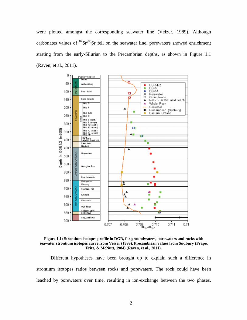
were plotted amongst the corresponding seawater line (Veizer, 1989). Although
carbonates values of 87
Sr/86
Sr fell on the seawater line, porewaters showed enrichment
starting from the early-Silurian to the Precambrian depths, as shown in Figure 1.1
(Raven, et al., 2011).
Figure 1.1: Strontium isotopes profile in DGR, for groundwaters, porewaters and rocks with
seawater strontium isotopes curve from Veizer (1999). Precambrian values from Sudbury (Frape,
Fritz, & McNutt, 1984) (Raven, et al., 2011).
Different hypotheses have been brought up to explain such a difference in
strontium isotopes ratios between rocks and porewaters. The rock could have been
leached by porewaters over time, resulting in ion-exchange between the two phases.
3
However, strontium isotope ratios of porewaters from the upper Ordovician in Figure 1.1
show a regular pattern that is not typical for leached rocks. That process would lead to an
87Sr/
86Sr value similar to that of the rock. That led to another possibility to explain the
difference in 87
Sr/86
Sr ratios: β-decay of 87
Rb over time in residual porewaters and/or in
the rock, causing a steady increase of 87
Sr that can be recovered from the porewater. As
the radionuclide is a monovalent cation, it does not behave the same way as strontium
does. Once decayed in the rock, strontium may be excluded from the original mineral as
it is not compatible, and would end up in the porewater. The decay being correlated with
time, it could be possible to create the regular pattern observed in Figure 1.1 if no other
sources of strontium or rubidium has mixed with porewaters. Finally, it is plausible that
none of these processes take place in this system, and the ingrowth of 87
Sr is simply
attributed to 87
Rb decay present in porewaters themselves.
1.2 Objectives
The overall objective of this project is (1) to determine the origin of the porewater
and (2) to explain the difference in isotopic signature of strontium in rocks and in
porewaters for the Upper Ordovician shales. Chosen samples of porewaters were
analyzed for strontium and rubidium isotopes. Corresponding rock samples were
sequentially leached to discriminate strontium and rubidium isotopes from the different
minerals. Data collected lead to a better understanding of the process in which the
porewaters became enriched in 87
Sr and were used (3) to determine the age of the rocks
and porewaters.
4
2.0 LITERATURE REVIEW
2.1 Study area
2.1.1 Location and topography
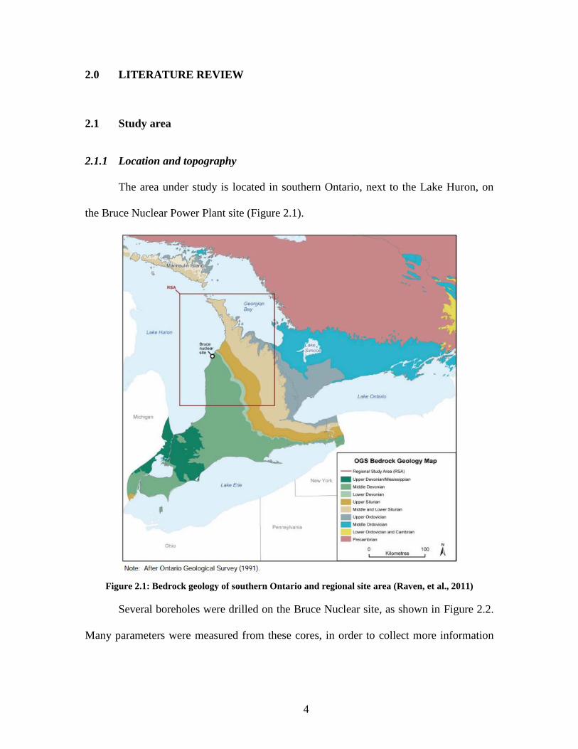
The area under study is located in southern Ontario, next to the Lake Huron, on
the Bruce Nuclear Power Plant site (Figure 2.1).
Figure 2.1: Bedrock geology of southern Ontario and regional site area (Raven, et al., 2011)
Several boreholes were drilled on the Bruce Nuclear site, as shown in Figure 2.2.
Many parameters were measured from these cores, in order to collect more information

5
on the feasibility of the project. In this thesis study, cores DGR-5 and DGR-6 were
emphasized.
Figure 2.2: Bruce nuclear site borehole locations (Raven, et al., 2011)
2.1.2 History of southern Ontario
The Ordovician rocks were formed during the Paleozoic Era, spanning from 541
to 252 million years before present. The Ordovician period covers the time between 485
and 443 million years before present. The beginning and the end of the period correspond
with major extinction events. At this time, the present eastern North America was located
in the tropics and was covered by inland seas. As a result, the southern Ontario Paleozoic
bedrock was formed by deposited marine sediments, from the Cambrian to the early
Carboniferous period (324 million years ago) (Armstrong & Carter, 2010).
6
2.1.3 Ordovician carbonates
The Ordovician carbonates, located in the middle Ordovician layers, are
subdivided into 2 groups: the Black River Group, which includes the Shadow Lake, Gull
River and Coboconk Formations, and the Trenton Group, which includes the Kirkfield,
Sherman Fall, Cobourg, and Collingwood Formations (Armstrong & Carter, 2010). These
rocks were formed during a major regional marine transgression that occurred after the
uplift and erosion of the Cambrian rocks. The transgression caused the overall sequence
of supratidal and tidal flat clastic/carbonates to lagoonal/shoal and deep shelf carbonates
(Kobluk & Brookfield, 1982). As this study focuses on the upper part of the middle
Ordovician, only the Cobourg Formation (Lower Member of the Lindsay Formation) and
the Collingwood Member (Lindsay Formation), both part of the Trenton Group, will be
described.
The Cobourg Formation is made of blue-grey to grey-brown fossiliferous
limestones and argillaceous limestones, with rocks ranging from very fine- to coarse-
grained (Armstrong & Carter, 2010). The Collingwood Member is formed of dark grey
and black calcareous shales, rich in organic carbon, overlying the fine-grained nodular
limestones of the Cobourg Formation (Armstrong & Carter, 2010). Mineralogical
analysis showed it is actually made of impure limestone or lime marlstone with high-
organics contents, causing its dark color (Macauley, Fowler, Goodarzi, Snowdon, &
Stasiuk, 1990).
2.1.4 Ordovician shales
The upper part of the Ordovician consists of orogeny-derived marine clastic
sediments (shale), deposited after the inundation of the Trenton Group. The area was

7
flooded after the carbonate platform of the Trenton Group collapsed, at the beginning of
the Taconic Orogeny. The resulting rocks are divided between 3 different formations:
Blue Mountain, Georgian Bay, and Queenston.
The Blue Mountain Formation is characterized by blue-grey to grey-brown shales
with variable amounts of siltstone, sandstone and limestone interbeds. The Georgian Bay
Formation is very similar, but has more greenish- to bluish-grey shale and contains more
fossils. Because of their similarities, the two formations are often combined and named
together. On the other hand, the 275-metre thick Queenston formation is characterized by
shale varying from red to maroon, with amounts of green shale, siltstone and sandstone
and limestone (Donaldson, 1989). The top of the formation shows a discontinuity caused
by a drastic sea level drop. This marine transgression caused the return of the carbonate-
forming conditions, in which the lower Silurian units formed (Manitoulin, Cabot Head,
Fossil Hill, Lions Head, Gasport, Goat Island and Guelph Formations).
2.1.5 Silurian units
The lower Silurian consists of intervals of sandstone, shale and limestone, formed
by the marine transgression previously explained. The upper section is characterized by
carbonate deposition, evaporites and related sediments (Armstrong & Carter, 2010). The
difference in composition is an indication of changes in the marine and sedimentary
environments. In facts, the Silurian rocks are the result of rapid basin subsistence and
arch uplift caused by the late Silurian Acadian Orogeny. The Michigan Basin became
more and more restricted, leading to evaporation of the water and precipitation of
carbonate, gypsum, anhydrite, halite and sylvite (Raven, et al., 2011). Occasional
8
intrusions of fresh marine water caused the repeating pattern of carbonates, evaporites
and argillaceous sediments observed in the Upper Silurian strata.
2.2 Strontium and rubidium dynamics
Isotopic systems are commonly used in geochronology and as tracers. The large
variety of radioisotopes allows dating objects from a few days to billions of years old,
making isotope systems powerful tools for scientists. Combined with stable isotopes, they
provide clues on past climates, origins of pollutants, and mixing rates of waters.
Strontium is the 16th
most abundant element in Earth’s crust, with a crustal
abundance of 370 ppm (Lide, 2005). It is a soft metal that substitutes for calcium in
numerous minerals such as apatite, gypsum, anorthite and carbonates, as they are both
divalent cations and have similar ionic radii (1.32 Å for Sr2+
, 1.14 Å for Ca2+
). In
minerals in which Si4+
is replaced by Al3+
, Sr2+
can substitute for K+, like in smectite and
vermiculite. The same process takes place in K-bearing minerals with rubidium and
potassium, as the elements are both monovalent and have similar ionic radii (1.66 Å for
Rb+, 1.52 Å for K
+) (Shannon, 1976). It is the case in muscovite, illite, and alkali
feldspars, for example (Capo, Stewart, & Chadwick, 1998). Their different valences also
have an impact on the hydrated radius on both ions. Because strontium is divalent, it will
attract more water molecules than rubidium, and thus be larger. The hydrated radii are
estimated to 2.28 Å for rubidium and 4.12 Å for strontium respectively (Ganguly, 2012).
Strontium and rubidium isotopes are widely used to identify geological processes
such as continental weathering and tectonic activity. Four stable strontium isotopes occur
in nature: 84
Sr (0.56%), 86
Sr (9.86%), 87
Sr (7.00%) and 88
Sr (82.58%). From these four,
only 87
Sr is radiogenic. It is a product of the radioactive β-decay of 87
Rb (Capo, Stewart,
9
& Chadwick, 1998) described in Equation 2.1 (Veizer, 1989). Rubidium has 2 isotopes:
85Rb (72.17%) and
87Rb (27.83%), the latter being the only radioactive species, with a
very long half-life of 4.88x10¹⁰
years. 87
Sr is commonly referred to as the “daughter”, and
87Rb, the “parent”.
𝑹𝒃𝟖𝟕 → 𝑺𝒓𝟖𝟕 + 𝜷− + ῡ + 𝑸 Equation 2.1
2.2.1 Isotope fundamentals
Most isotopes are expressed as a relative atomic ratio to the most abundant
isotope for each element. They are usually measured with respect to references of a
known isotopic content. For example, 18
O/16
O is expressed in comparison to Vienna
Standard Mean Ocean Water (VSMOW) for water samples and to Vienna Pee Dee
Belemnite (VPDB) for carbonates. The dimensionless ratio, called delta (δ), is expressed
in parts per thousand, or permil (‰) and is calculated according to Equation 2.2 (Clark &
Fritz, 1997):
𝜹 (‰) = (𝑹𝒔𝒂𝒎𝒑𝒍𝒆
𝑹𝒔𝒕𝒂𝒏𝒅𝒂𝒓𝒅− 𝟏) ∗ 𝟏𝟎𝟎𝟎
Equation 2.2
where Rsample and Rstandard are the atomic ratios in the sample and reference material.

10
In the case of strontium isotopes, it is possible to use the same notation as
described above, as in Equation 2.3.
𝜹 𝑺𝒓𝟖𝟕 = ([ 𝑺𝒓𝟖𝟕 / 𝑺𝒓𝟖𝟔 ]
𝒔𝒂𝒎𝒑𝒍𝒆
[ 𝑺𝒓𝟖𝟕 / 𝑺𝒓𝟖𝟔 ]𝒔𝒕𝒂𝒏𝒅𝒂𝒓𝒅
− 𝟏) ∗ 𝟏𝟎𝟎𝟎
Equation 2.3
In this specific case, absolute strontium isotope ratios can be measured directly with new
technologies, without using the delta notation. The international reference
NIST SRM-987 (87
Sr/86
Sr = 0.71025) is used to calibrate instruments in this situation. As
a result, in most publications, strontium isotopes are expressed in absolute ratios rather
than with the δ notation.
2.2.2 Strontium cycle
Depending on their nature, rocks may contain high levels of strontium. Sr is
released from rocks by weathering and erosion processes, including actions from winds,
animals and plants. Water is the main vector for Sr to reach rivers, lake, and eventually
oceans – the largest reservoir of dissolved Sr – and to be deposited in marine carbonates.
Tectonic activity and volcanism are then responsible for recycling crustal material.
Isotopic signatures of strontium may be different from one reservoir to another, as shown
in Figure 2.3.

11
Figure 2.3: Strontium fluxes and 87
Sr/86
Sr in reservoirs (Hodell, Mead, & Mueller, 1990)
Alterations of isotopic signatures cannot be explained by isotopic fractionation in
a sedimentary basin system, as it is unlikely to happen. The mass difference between the
different isotopes is too low (87
Sr is only 1.1% heavier than 86
Sr) for physical and
chemical processes to use one preferentially. However, interactions between rock and
water may change the ratio, depending on the mineralogy. For example, a clay mineral
containing high levels of Rb will undergo 87
Rb decay over time, thus the 87
Sr/86
Sr ratio in
the clay mineral will rise. Water-rock interactions could then be responsible for an
increase of the 87
Sr/86
Sr in the water. On the other hand, the strontium isotopes ratio in a
carbonate mineral containing very low levels of Rb+ will not get significantly altered over
time.
In the case of sedimentary rocks deposited in marine environment, rocks and
porewaters have the same 87
Sr/86
Sr ratio as the seawater at the time of deposition (Faure
& Gunter, 1991). A higher ratio measured in the water could indicate some mixing with
an external source of rubidium or enriched strontium. It is then possible to conclude that

12
Sr isotopes ratios in the different reservoirs are mainly altered by the presence of 87
Rb,
which decays over time, and by mixing with sources of different ratios.
In oceans, the residence time of Sr is between 2 and 4 million years (Hodell,
Mead, & Mueller, 1990), which is much longer than the oceanic mixing rate of a few
thousand years (Veizer J. , 1992). This explains why strontium concentration is relatively
uniform in oceans.
2.2.3 Rubidium cycle
Because of its very large radius, rubidium is excluded from crystals when magma
cools down. Being sequentially excluded, late-stage magmatic products tend to be highly
concentrated in rubidium (Anderson, 1989). Examples are pegmatite, biotite and
muscovite, which could contain more than 1000 ppm of rubidium. As a result, Rb is
present in greater concentration in crustal material than in mantle minerals, with which it
is virtually incompatible. Therefore, weathering products from the crust are enriched in
87Rb and become more radiogenic over time, leading to greater values of
87Sr/
86Sr. This
corresponds to the high strontium isotopes ratio shown in Figure 2.3.
Rubidium moves between rocks and water the same way strontium does.
However, it rarely forms actual minerals. It is adsorbed onto clay minerals such as illites
more strongly than K+. Of course, its size and valence will not allow it to be incorporated
in minerals such as carbonates like strontium does. Rubidium substitutes for potassium in
minerals such as orthoclase and biotite.
The chemistry of strontium and rubidium, as previously explained, is responsible
for various concentrations of these two elements in the different reservoirs and types of
rocks, as shown in Table 2.1.

13
Table 2.1: Average concentrations of calcium, strontium, potassium and rubidium in different
reservoirs.
Ca (ppm) Sr (ppm) K (ppm) Rb (ppm) Reference
Average crust 41 000 370 21 000 90 (Sposito, 1989)
Modern Sea Water 414 000 7 620 425 000 110 (Holland, 1984)
Deep-Sea Carbonate 312 400 2 000 2 900 10
(Faure G. , 1986) Carbonate 302 300 610 2 700 3
Shale 22 100 300 26 600 140
Deep-Sea Clay 29 000 180 25 000 110
2.2.4 Rb-Sr dating
Because 87
Rb is radioactive, it can be used, combined with its daughter 87
Sr, to
date minerals. With a constant of (1.3968 ± 0.0027)x10-11
decay per year (Rotenberg,
Davis, Amelin, Ghosh, & Bergquist, 2012), this isotopic system could technically be used
to date material older than the age of the universe, 13.77x10⁹ years old (National
Aeronautics and Space Administration, 2012). The rate of decay is directly proportional
to the number of atoms, expressed by:
𝑑𝑁
𝑑𝑡∝ 𝑁
where N is the amount of radioactive parent isotope. Because the amount of parent
isotope is constantly diminishing, dN/dt has a negative value. The decay constant, λ, also
has to be considered to establish the number of decays:
𝑑𝑁
𝑑𝑡= −𝜆𝑁

14
By rearranging and integrating the previous equation:
∫𝑑𝑁
𝑁= −𝜆 ∫ 𝑑𝑡
𝑡
𝑡0
𝑁
𝑁𝑜
𝑙𝑛 (𝑁
𝑁0) = −𝜆(𝑡 − 𝑡0)
Replacing t0 by its real value (0), we obtain the following equation:
𝑵 = 𝑵𝟎𝒆−𝝀𝒕 Equation 2.4
where N is the amount of radioactive parent isotope at time t, N0 is the initial amount of
radioactive parent isotope, t is the elapsed time, and λ is the decay constant. The amount
of daughter isotopes, D, is then expressed by the difference between N0 and N:
𝑫 = 𝑵𝟎 − 𝑵 Equation 2.5
Thus, by replacing N in Equation 2.5 by rearranged Equation 2.4, it is possible to get a
formula that directly leads to the amount of daughter isotope from decay:
𝑫 = 𝑵𝟎 − 𝑵 = 𝑵𝒆𝝀𝒕 − 𝑵 = 𝑵(𝒆𝝀𝒕 − 𝟏) Equation 2.6
This last equation is considered true in a case where no daughter isotope is found
initially. When it is not the case, the initial amount of daughter isotope, D0, has to be
taken into consideration in calculation.
𝑫 = 𝑫𝟎 + 𝑵(𝒆𝝀𝒕 − 𝟏) Equation 2.7

15
When applied to the Rb-Sr dating method, Equation 2.7 becomes Equation 2.8:
(𝑺𝒓𝟖𝟕
𝑺𝒓𝟖𝟔)
𝒕𝒐𝒕𝒂𝒍
= (𝑺𝒓𝟖𝟕
𝑺𝒓𝟖𝟔)
𝒊𝒏𝒊𝒕𝒊𝒂𝒍
+ (𝑹𝒃𝟖𝟕
𝑺𝒓𝟖𝟔) (𝒆𝝀𝒕 − 𝟏)
Equation 2.8
Because it is impossible to measure D0, it has to be calculated from a graph, where it
corresponds to the intercept (Figure 2.4). In the case of a sedimentary basin, this will
likely correspond to the isotopes ratio of the seawater at the time of deposition
(Chaudhuri & Clauer, 1992). From Equation 2.8, the age can be calculated by reporting
the analytical value of 87
Sr/86
Sr on the Y-axis and 87
Rb/86
Sr on the X-axis for different
components of the same material in an isochron, as shown in Figure 2.4. Knowing the
value of the slope, it is possible to solve for t, which corresponds to the age of the
material.
Figure 2.4: Rb-Sr isochron (Nelson, 2013)
From Figure 2.4, it is evident that the amount of 87
Sr at the time of measurement
depends on the original content in rubidium. Therefore, knots A, B, C and D represent
different components of a rock: calcite, whole rock, K-feldspar and biotite, for example,
A B C D
tx
t0
t0
t0
16
with increasing Rb original content. Of course, this situation represents a case where no
other sources of rubidium or strontium have mixed with the system. The main criterion in
geochronology is that the studied system was closed since its formation, therefore there
was no gain or loss of neither parent nor daughter isotopes by external sources or by
diffusion. Also, the different minerals taken from the rock to build the isochron must
have been formed and deposited at the same time. The minerals must have formed in
chemical equilibrium one to another in order to make a trustable isochron.
2.2.5 Evolution of 87
Sr/86
Sr over geological time
Modern seawater has an 87
Sr/86
Sr value of 0.7090, which represents a mixture of
both depleted oceanic (0.705) and continental enriched crust (˃0.710) (Figure 2.3). The
original bulk Earth’s value of 0.69899 is directly derived from meteorites
(Papanastassiou, Wasserburg, & Burnett, 1969). It is also referred to as the basaltic
achondrite best initial ratio (BABI). The mantle’s ratio has continuously been increasing
over time, as 87
Rb is constantly decaying into 87
Sr (see Figure 2.5). After the crustal
formation, the curve for the mantle became depleted in rubidium since the ion is
concentrated in the crust. As mentioned in section 2.2.3, rubidium is excluded from
minerals when magma cools down, enriching crustal rocks. This phenomenon is
responsible for the steep curve of the crust, and depletion of the Rb/Sr ratio in the mantle
in Figure 2.5. When a modern melt is derived from partial melting of the mantle, its
87Sr/
86Sr value is lower than a melt from crustal rocks would be.

17
Figure 2.5: Estimated evolution of 87
Sr/86
Sr of the Earth’s upper mantle, assuming a large-scale
melting event producing granitic-type continental rocks at 3.0 Ga b.p. (Wilson, 1989)
Modern values of strontium isotopes ratios are not as linear as in Figure 2.5. They
are controlled by different geological processes. Figure 2.6 shows variations of 87
Sr/86
Sr
ratio in seawater throughout Phanerozoic Time. Those variations have been explained by
high volcanism and spreading ridges, causing the release in oceans of 87
Sr-depleted
magmas. On the other hand, increases in 87
Sr are usually caused by weathering of
continent by glaciers, as observed in the late Cenozoic sediments (Clark & Fritz, 1997).

18
Figure 2.6: Strontium isotopes in seawater through time (Burke, et al., 1982)
Geochemistry of elements is also considered to explain variations of 87
Sr/86
Sr in
groundwaters, rivers and lakes, as the ratio is directly linked to the composition of
terrains. 87
Sr being the daughter of 87
Rb, the ratio will be directly linked to the potassium
content, which is high in clays and low in limestone once the water has reached
equilibrium with the rock. Thus, waters sitting on different terrains may have
significantly different isotopic signatures.
2.3 Mineral dissolution
Samples selected for this study are located just above the proposed repository,
which is 680 m deep (Figure 2.7). Emphasis was put on rocks from the upper and the top
of the middle Ordovician layers, including Queenston, Georgian Bay, Blue Mountains,
Collingwood and Cobourg formations, as the divergence between the Sr isotopes ratio in
rocks and porewaters happens mainly in these layers (ref. Figure 1.1). Shale and

19
argillaceous limestone are the main type of rocks found in the upper and middle
Ordovician, respectively.
Figure 2.7: Stratigraphy of the Bruce nuclear site (Raven, et al., 2011)
Major components of the rock were previously identified with various techniques
(electron microprobe, XRD, SEM/EDS, lithogeochemistry) (Raven, et al., 2011). Results
are shown in Figure 2.8.

20
Figure 2.8: Content weight of major components (Raven, et al., 2011)

21
Knowing the composition of the rocks was essential to determine the procedure to
be used to dissolve specific minerals. Based on Figure 2.8, the main components (calcite,
dolomite, and silicates) were targeted in the dissolution sequence, as they are found in
various concentrations at the studied depths. This choice of sequence is also consistent
with the site history. Calcite has been deposited at the bottom of the sea along with clay
minerals that likely were brought by erosion of the continent. Later on, Silurian brines
have infiltrated the rocks, causing dolomitization. Since the three mineral phases have a
different history and mechanism of formation, it was sensible to separate them.
Whole-rock dissolution is a widely used technique around the world to determine
mineral content and isotopes. Several research groups have dissolved carbonate rocks in
order to get strontium isotopes ratios. By doing so, it is possible to extract strontium from
every phase and have a better understanding of interactions between them. Different
leaching sequences have been tried to separate calcite from dolomite and silicates. The
main idea is to dissolve the entire sample in a specific sequence:
- Remove labile, adsorbed ions, and water soluble evaporites;
- Dissolve calcite;
- Dissolve dolomite and other carbonates;
- Dissolve silicates.
The removal of labile and exchangeable ions is necessary in order to avoid
contamination of the Sr ratio in further leachates. Ammonium acetate solution (1M) is
commonly used to do this (Jacobson, Blum, Page Chamberlain, Poage, & Sloan, 2002).
However, ammonium acetate is known to form complexes with calcium, which may
22
cause some calcite dissolution (Bailey, McArthur, Prince, & Thirlwall, 2000). Deionized
water happens to be an appropriate alternative to avoid this problem (Gosselin, Harvey,
Frost, Stotler, & Macfarlane, 2004).
Calcite dissolution can be achieved by leaching with acetic acid (Tessier, Campbell, &
Bisson, 1979) (Lerouge, et al., 2010). A rapid leach with low-concentration acetic acid –
usually 5 to 10% ‒ is proven to maximize dissolution of calcite over dolomite (Sharp,
Creaser, & Skidmore, 2002).
Treatment with HCl is common when it comes to dissolve all types of carbonates.
However, hydrochloric acid will also remove a significant amount of Sr from the surface
of clay particles without dissolving any of the silicate phases (Clauer, Chaudhuri, Kralik,
& Bonnot-Courtois, 1993). HCl also attacks hydrated oxides, sulfides and phosphates
(Gosselin, Harvey, Frost, Stotler, & Macfarlane, 2004).
The final step includes dissolution of the remaining silicates. Most of the time, a mixture
of nitric, hydrofluoric and perchloric acid is used (Jacobson, Blum, Page Chamberlain,
Poage, & Sloan, 2002) (Sharp, Creaser, & Skidmore, 2002).
2.4 Previous work on the DGR cores
2.4.1 Porewater solutes extraction
Porewaters were extracted in 2008 using the crush and leach technique. After
being crushed to 2-4 mm grain size, samples were heated to 150°C under vacuum to
extract porewaters. This was followed by a deionized water leach of the same crushed
rocks, for 60 days, in order to recover ions from porewaters. The resulting extraction
factors are shown in racted under vacuum.

23
Table 2.2. An aliquot of the leaching water was then taken up for geochemical
analyses. Original ion concentrations in porewaters were calculated by dividing the mass
of ion in the leachate by the mass of porewater extracted under vacuum.
Table 2.2: Extraction factors for porewaters
Sample ID
Mass of
porewater
extracted (g)
Mass of water
added for
leaching (g)
Extraction
factor
DGR5-497.50 1.5186 29.9841 19.74
DGR5-514.22 1.2865 32.2265 25.05
DGR5-525.57 1.2441 36.0370 28.97
DGR5-557.65 1.6867 32.3357 19.17
DGR5-564.96 0.7955 38.8617 48.85
DGR5-598.37 1.4268 35.3841 24.80
DGR5-625.23 1.4625 33.0629 22.61
DGR5-649.57 1.6137 32.6206 20.21
DGR6-654.12 1.4873 36.5946 24.60
DGR6-661.83 1.2537 37.9262 30.25
DGR6-662.17 0.6324 37.2685 58.93
DGR6-662.82 1.3021 36.9034 28.34
DGR5-671.30 1.3404 34.6608 25.86
DGR6-683.25 1.2299 36.7836 29.91
DGR5-683.57 1.0652 38.2880 35.94
DGR5-697.85 1.1594 35.6760 30.77
DGR6-697.97 1.4332 37.0231 25.83
DGR5-715.60 1.3173 37.8426 28.73
DGR5-724.90 2.7652 39.5468 14.78
DGR5-731.02 2.0117 36.8032 18.30
DGR5-734.06 1.0753 35.1175 32.66
2.4.2 Preliminary analyses
Some preliminary strontium isotopes analyses were done a few samples from the
upper Ordovician shale and middle Ordovician limestone, in 2010. Once porewaters were
extracted and ions were leached, a few grams of rocks were rinsed with deionized and

24
dried before being crushed to powders and leached with 5% acetic acid, for 20 minutes,
in an ultrasonic bath, to dissolve calcite. In addition, 2 samples from the upper
Ordovician and 2 samples from the middle Ordovician were rinsed, dried, and completely
dissolved to analyze the whole rock strontium isotopes ratio. Results are shown in Figure
2.9.
Figure 2.9: Strontium isotopes in groundwater, porewater and rocks (Raven, et al., 2011)
Acetic acid leachates (black triangles) from the upper and middle Ordovician
show strontium isotopes ratios falling close to the seawater line, indicating carbonates
likely originate from the seawater. Whole rock values (purple triangles) are more

25
enriched in shales than in limestones, which is expected as they contain more clay
minerals.
Porewater values from the shales show enrichment in 87
Sr that neither is in
equilibrium with carbonate phases (acetic acid leachable) nor it is with whole-rocks
values. This quick analysis suggests that simple leaching of the rocks by pore fluids
cannot be a valid explanation for the enrichment of radiogenic strontium in porewaters.

26
3.0 METHODOLOGIES
3.1 Sample selection
The focus of this study was put on DGR 5 and 6 cores, more specifically in the
upper Ordovician shales and the Cobourg formations. Table 3.1 shows samples used for
the project with respect to their formation and depth. All available samples were picked
for further analyses. Formations and depths relative to DGR-1/2 are shown in Figure 3.1.
Results will later be expressed relative to DGR-1/2.
Figure 3.1: Formations and depths relative to DGR-1/2

27
Table 3.1: Samples availabilities and associated formations
Formation Core Depth
(mLBGS)
Actual
Depth
(mBGS)1
Depth
relative to
DGR 1/2
Rock
sample
Porewater
sample
Queenston DGR5 497.50 456.52 458.01 √ √
Queenston DGR5 514.22 472.36 473.82 √
Queenston DGR5 525.57 483.14 484.59 √ √
Queenston DGR5 557.65 513.72 515.12 √
Georgian Bay DGR5 564.96 520.69 522.20 √ √
Georgian Bay DGR5 598.37 552.59 554.92 √ √
Georgian Bay DGR5 625.23 578.28 581.28 √ √
Georgian Bay DGR5 649.51 601.56 605.17 √
Georgian Bay DGR6 654.12 571.89 582.42 √
Georgian Bay DGR6 661.83 578.67 589.11 √
Georgian Bay DGR6 662.17 579.21 589.41 √ √
Georgian Bay DGR6 662.82 578.38 589.98 √
Blue Mountain DGR5 671.30 622.55 625.33 √
Georgian Bay DGR6 683.25 596.39 607.67 √
Blue Mountain DGR5 683.57 634.43 636.57 √
Blue Mountain DGR6 697.79 608.60 619.36 √
Blue Mountain DGR5 697.85 648.30 649.71 √
Cobourg DGR5 715.60 665.60 666.57 √ √
Cobourg DGR5 719.91 669.81 671.01 √
Cobourg DGR5 724.90 674.68 676.15 √
Cobourg DGR5 731.02 680.65 682.45 √ √
Cobourg DGR5 734.06 683.61 685.58 √ √ 1 The difference between depths and actual depths is attributed to angle when cores were drilled (ref. Figure 2.2)
Porewaters were extracted in 2008 from crushed rocks (2-4 mm) as described in
section 2.4.1 and stored in 15 mL plastic tubes until ready for analyses. Crushed rocks
samples were left in deionized water and stored in 50 mL Falcon tubes. All samples were
stored in cardboard boxes, kept away from heat and light until the beginning of this
project in 2013.

28
3.2 Preparation
A few grams of the crushed rock samples were taken out of the Falcon tubes,
rinsed with deionized water and dried at 70°C overnight. They were then taken to the
crushing room to be pulverized to fine powders with the help of a disk mill. Between
each sample, the equipment was rinsed with water, ethanol, and dried out. Silica beads
were crushed in the disk mill in order to clean the pores before it was rinsed again with
water, ethanol, dried, and pre-contaminated with the next sample. After being crushed,
samples were stored in 15-mL plastic tubes until ready for analyses.
Rock and porewater samples were transported at the Isotope Geochemistry and
Geochronology Research Centre (IGGRC) at Carleton University for strontium isotopes
analysis. All laboratory work related to strontium isotopes took place in the IGGRC clean
laboratory, using ultra clean Teflon containers and instruments.
In order to extract strontium from the different components of the rock, samples
underwent sequential leaching based on information from section 2.3. The time of
reaction and the amount of chemical required for each step was based on previous
experiments done at the IGGRC. Selected chemical were nanopure water, 5% acetic acid,
6N HCl and a mixture of 50% HF-12N HNO3. Various times of leaching were tried to
find the optimal dissolution process in order to separate adsorbed ions, calcite, dolomite
and silicates. A reference value was available to confirm the validity of the method: the
strontium isotopes ratio for the acetic acid leachate of the DGR3-687.10 had to be of
0.7080, which corresponds to the seawater value (Spencer, 2013). Once this value was
obtained for this sample, the method was applied on all other rock samples.

29
3.3 Analytical procedure
3.3.1 Rock samples
Powdered rock samples were weighted. Masses are indicated in Table 3.2.
Samples were run by batches of 3 at the time, for logistic reasons. Each batch took
3 weeks to analyze for strontium isotopes. Only 100 mg of the first samples were used to
compare the quality of the signal on the mass spectrometer used later on. Since the
quality of the signal was much better when using 200 mg of samples, it was decided to
keep this amount for other batches.
Table 3.2: Masses of rock samples
Sample ID Mass (mg)
DGR5-497.50 100.17
DGR5-525.57 200.96
DGR5-564.96 199.59
DGR5-598.37 198.36
DGR5-625.23 199.97
DGR6-662.17 199.17
DGR5-715.60 201.87
DGR5-719.91 199.08
DGR5-731.02 201.12
DGR5-734.06 200.99
Samples were put in a 15 mL Teflon container with 3 mL of nanopure water, capped and
left in an ultrasonic bath for 20 minutes before being taken out to rest for 5 minutes. The
mixtures were transferred in tubes and were centrifuged for 4 minutes. Water
supernatants were pipetted, transferred in pre-labelled 5 mL Teflon containers and stored.
The remaining powders were mixed with 3 mL of 5% acetic acid, put back in their
original Teflon containers and left in the ultrasonic bath for 20 minutes again. After being

30
taken out to rest for 5 minutes, the mixtures were transferred again in tubes to be
centrifuged for 4 minutes. Acidic supernatants were extracted with pipettes, transferred in
new pre-labelled 5 mL Teflon containers and stored. The remaining powders were mixed
with 3 mL of 6N HCl and went through the same procedure again. After supernatants
were removed and stored, the powders were entirely dissolved in a mixture of
50% HF - 12N HNO3. Samples were capped and left on a hotplate at 140°C until
complete dissolution.
After 6 days, the hot containers were uncapped and placed on the hotplate to evaporate to
dryness. A few drops of 7N HNO3 were added to the residues and evaporated, and then
3 mL of 6N HCl were added. The containers were capped and left on the hotplate
overnight. On the following day, all 12 containers (4 per sample – one for each leachate)
were opened and evaporated at 90 C. A few drops of 7N HNO3 were added in all
containers and dried down, and samples were redissolved in 3 mL of 2.5N HCl. All
containers were capped and left on the hotplate at 90°C overnight.
On the following morning, samples were divided in 2 subsamples of 1.5 mL each.
The first portion was dried, dissolved in 1.5 mL 7N HNO3 and stored in clean 15 mL
plastic tubes for further ICP analyses. The second subsample underwent strontium
extraction, using Dowex 50-X8 Cation resin, following the procedure described in
Appendix A. The strontium enriched phases were collected in clean pre-labelled Teflon
containers, left on a hotplate at 90°C to dry overnight, and spotted with 7N HNO3 again
on the following day to remove all traces of organic molecules. All containers were
capped and stored until ready for the next step.

31
Samples were then brought to the mass spectrometer laboratory. They were
dissolved in 4.2 µL of concentrated H3PO4, and 3 µL of each were put on single tantalum
filaments with a pipette and dried. An additional filament was prepared with
NIST SRM-987 standard (87
Sr/86
Sr = 0.710239 ± 0.000014) (Carleton University, 2012).
Filaments were inserted on the carrousel and put in the thermal ionization mass
spectrometer (TIMS). Samples were analyzed under vacuum on the following days. Table
3.3 shows analytical specifications of the instrument.
Table 3.3: Analytical parameters for the thermal ionization mass spectrometer
Brand
Filament
Fisher Scientific®
Single Tantalum
Current 2600-3000 mA
Temperature 1350-1400°C
Target signal 1.0 V
Number of measurements 100
Samples preserved for ICP analysis underwent proper dilution with 1% HNO3 and
were passed through 0.45 µm nitrocellulose filters. Cations (Na+, K
+, Mg
2+, Ca
2+ and
Sr2+
) were measured by Inductively Coupled Plasma Optical Emission Spectroscopy
(ICP-OES) using a Varian (Agilent)® Vista-Pro. Rubidium isotopes were determined by
Inductively Coupled Plasma Mass Spectrometer (ICP-MS). Specifications for both
instruments are shown in Table 3.4 and Table 3.5.

32
Table 3.4: Analytical parameters for the ICP-OES
Brand Varian (Agilent) Vista Pro®
Detector CCD
View Radial
RF Power 1.35 kW
Plasma Gas Flow 15 L/min
Auxiliary Gas Flow 1.5 L/min
Carrier Gas Flow 0.8 L/min
Sample Uptake Rate 1.0 mL/min
Table 3.5: Analytical parameters for the ICP-MS
Brand Agilent 7700x Quadrupole®
RF Power 1.50 kW
Plasma Gas Flow 15 L/min
Auxiliary Gas Flow 1.5 L/min
Carrier Gas Flow 1.0 L/min
Sample Uptake Rate 0.10 mL/min
3.3.2 Porewater samples
Porewater samples underwent proper dilutions with 1% HNO3 and were analyzed
for their content in sodium, potassium, magnesium, calcium and strontium with the ICP-
OES. Analytical parameters are described in Table 3.4. Diluted samples were also run on
the ICP-MS, with the analytical parameters described in Table 3.5. Appropriate standards
were prepared as well for all ions.
Strontium isotopes were also measured in porewaters. To do so, 1.5 mL of each
sample was dried down on a 90°C hotplate, in a clean Teflon beaker, at the IGGRC
laboratory. Once dried, residues were spotted with 7N HNO3 and dried again. 1.5 mL of
2.5N HCl was added to each beaker in order to perform strontium separation with Dowex
50-X8 cation exchange resin, as described in Appendix A. Strontium enriched phases
were collected in pre-labelled clean Teflon containers, were dried on a 90°C hotplate, and

33
redissolved in 4.2 µL H3PO4. 3 µL of each samples were deposited on single tantalum
filaments and dried. All samples along with a standard were put in the TIMS and
analyzed on the following day. Analytical parameters are described in Table 3.3. A total
of 21 porewater samples were analyzed (ref. Table 3.1).
3.4 Calculations
3.4.1 Strontium isotopes ratios
Strontium isotope ratios can be directly measured by thermal-ionization mass
spectrometer. In fact, 2 ratios are measured: 88
Sr/86
Sr, and 87
Sr/86
Sr. The first one is called
the normalizing ratio, as it should be constant in the environment. Neither 88
Sr nor 86
Sr
are radioactive or radiogenic, so their ratio must be 8.375 in any sample. In parallel, the
second ratio is measured. 87
Sr being radiogenic, the ratio varies from one sample to the
other. When the instrument measures a value different than 8.375 for 88
Sr/86
Sr, the
software applies a correction factor over the 87
Sr/86
Sr value, to correct for the deviation.
When measuring, filaments can reach a temperature of 1 400°C that can cause
fractionation, explaining any deviation from the value. To ensure this factor is correct, a
third ratio (84
Sr/86
Sr) is measured. Just like strontium 88 and 86, strontium 84 is constant
in the environment, thus the expected 84
Sr/86
Sr ratio is 0.05649. The measured ratio
multiplied by the correction factor should then always be equal to 0.05649.
The TIMS also corrects for the presence of 87
Rb, which causes interferences in the
measurement of 87
Sr as both species have the same mass. If the concentration of rubidium
is very low, it is possible for the detector to measure 85
Rb, to transform it into an
87Rb/
86Sr ratio, and to substract this value from the measured
87Sr/
86Sr ratio.

34
100 measurements are being taken of each sample. The software uses standard statistical
parameters in order to calculate the actual values and uncertainties for each sample.
Therefore, the arithmetic mean, standard deviation and standard error are calculated for
each sample. Reported values for strontium isotopes ratios show the mean of these 100
measurements, and the uncertainty represents the standard error multiplied by 2. Since
strontium isotope ratios are absolute measurements, no dilutions factors have to be taken
in consideration.
3.4.2 Rubidium isotopes
Rubidium isotopes were measured with the ICP-MS, as mentioned previously.
The appropriate standard solutions are prepared and a calibration curve is calculated. To
avoid dealing with mass interferences between 87
Sr and 87
Rb, 85
Rb is measured and the
concentration is back-calculated with the calibration curve. Since the abundance of each
isotope is well known, 87
Rb could be determined by multiplying the concentration of 85
Rb
by the abundance factor, which is 0.3856, as shown in Equation 3.1. In addition to that,
the obtained result is multiplied by the dilution factor (DF) for both rocks and porewater
samples. For porewaters, another factor has to be considered to get the original
concentration of isotopes. When they were extracted, porewaters were diluted by factors
shown in Table 2.2. This second factor, the extraction factor (EF) has to be applied on the
calculated concentrations as well.
[ 𝑹𝒃𝟖𝟕 ](𝒑𝒑𝒎)
= (𝑹𝒃(𝒄𝒐𝒖𝒏𝒕𝒔)
𝟖𝟓 − 𝑰𝒏𝒕𝒆𝒓𝒄𝒆𝒑𝒕
𝑺𝒍𝒐𝒑𝒆) ∗ 𝟎. 𝟑𝟖𝟓𝟔 ∗ 𝑫𝑭(∗ 𝑬𝑭)
Equation 3.1
35
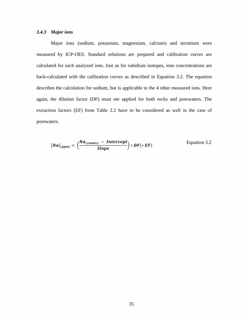
3.4.3 Major ions
Major ions (sodium, potassium, magnesium, calcium) and strontium were
measured by ICP-OES. Standard solutions are prepared and calibration curves are
calculated for each analyzed ions. Just as for rubidium isotopes, ions concentrations are
back-calculated with the calibration curves as described in Equation 3.2. The equation
describes the calculation for sodium, but is applicable to the 4 other measured ions. Here
again, the dilution factor (DF) must me applied for both rocks and porewaters. The
extraction factors (EF) from Table 2.2 have to be considered as well in the case of
porewaters.
[𝑵𝒂](𝒑𝒑𝒎) = (𝑵𝒂(𝒄𝒐𝒖𝒏𝒕𝒔) − 𝑰𝒏𝒕𝒆𝒓𝒄𝒆𝒑𝒕
𝑺𝒍𝒐𝒑𝒆) ∗ 𝑫𝑭(∗ 𝑬𝑭)
Equation 3.2

36
4.0 RESULTS AND DISCUSSION
4.1 Geochemistry
4.1.1 Rocks
Sodium, potassium, rubidium, calcium, magnesium, and strontium were analyzed to
determine their amount in each sample, with the methodology described in 3.3. In rock
samples, cations were expected to be representative of the lithology. Furthermore, they
were used to determine the validity of the leaching sequence. Measurements were
corrected for dilutions, and final concentrations are presented in
Table 4.1. For each element, concentrations are normalized for one kilogram of
rock (ref. Table 3.2). Additionally, rubidium concentrations were calculated from 85
Rb
measurements, as described in Section 3.4.2. Uncertainties are estimated to 1% for all
concentrations.

37
Table 4.1: Concentrations of ions in rocks
Sodium (mg/kg) Potassium (mg/kg) Rubidium (mg/kg)
Sample ID H2O
leachate AcOH
leachate HCl
leachate HF/HNO3
dissolution H2O
leachate AcOH
leachate HCl
leachate HF/HNO3
dissolution H2O
leachate AcOH
leachate HCl
leachate HF/HNO3
dissolution
DGR5-497.50 154 62.1 31.6 478 854 232 1 389 23 991 3.36 1.06 9.37 104
DGR5-525.57 124 70.1 54.3 544 540 550 1 250 19 481 1.49 0.89 6.92 133
DGR5-564.96 55.7 35.5 39.1 323 236 379 570 19 419 0.65 0.87 3.20 99.4
DGR5-598.37 108 44.2 29.8 101 355 467 713 13 065 1.28 0.88 5.52 30.3
DGR5-625.23 167 44.0 24.1 209 453 426 640 13 339 0.99 0.79 5.19 42.1
DGR6-662.17 27.4 48.3 47.2 1 105 103 297 435 15 002 0.68 0.52 2.48 80.3
DGR5-715.60 32.7 68.6 129 106 109 189 372 7 351 0.33 0.29 1.39 31.7
DGR5-719.91 28.3 47.6 94.0 65.7 85.4 129 227 5 049 0.27 0.24 1.13 24.7
DGR5-731.02 27.2 89.5 68.9 100 134 250 313 9 008 0.40 0.47 1.65 39.9
DGR5-734.06 35.2 49.6 56.9 55.7 93.0 129 193 5 161 0.28 0.26 1.07 20.1
Magnesium (mg/kg) Calcium (mg/kg) Strontium (mg/kg)
Sample ID H2O
leachate AcOH
leachate HCl
leachate HF/HNO3
dissolution H2O
leachate AcOH
leachate HCl
leachate HF/HNO3
dissolution H2O
leachate AcOH
leachate HCl
leachate HF/HNO3
dissolution
DGR5-497.50 329 6 595 22 946 6 502 385 94 549 4 457 303 4.34 99.6 9.7 26.3
DGR5-525.57 77.9 939 6 129 6 695 765 94 396 42 940 2 636 5.16 134 29.4 22.7
DGR5-564.96 73.7 2 724 10 826 5 485 722 79 614 62 569 5 055 4.56 91.6 28.8 21.1
DGR5-598.37 143 1 404 2 612 1 398 327 14 784 28 280 335 3.32 65.6 15.0 7.46
DGR5-625.23 65.4 1 625 2 018 1 631 465 22 451 12 981 338 5.48 32.9 13.9 8.12
DGR6-662.17 25.5 802 7 777 4 397 245 129 498 64 060 4 648 1.66 213 65.0 24.7
DGR5-715.60 17.5 605 3 809 1 646 860 122 112 173 748 17 845 2.06 197 282 22.9
DGR5-719.91 21.7 637 3 729 1 262 1 190 129 636 175 246 14 787 2.62 181 253 17.1
DGR5-731.02 30.0 1 008 5 799 1 920 559 187 283 136 010 8 540 2.44 260 197 17.0
DGR5-734.06 24.6 797 2 803 1 024 1 741 175 815 160 419 10 853 2.84 223 219 13.3

38
As expected, concentrations in water leachates are very low compared to the other
ones. This leach can be considered as a simple wash, but could also have dissolved
cations adsorbed onto surfaces of clays and other minerals. Traces of celestite detected in
those samples (Raven, et al., 2011) could also have been dissolved by the water leachate
(Bailey, McArthur, Prince, & Thirlwall, 2000). Moreover, high concentrations of sodium
in water leachates were measured in the upper part (DGR5-497.50 to DGR5-625.23).
Those values are consistent with previous observations of halite in the upper Ordovician
shales, with concentrations decreasing through depth (Jackson & Murphy, 2011).
The acetic acid and hydrochloric acid leachates are highly enriched in divalent
cations. The purpose of doing both leaches was to preferentially dissolve calcite over
other carbonates (mainly dolomite) with acetic acid, and to dissolve all of the other
carbonates with HCl. Magnesium concentrations in both leachates lead to believe
dolomite is concentrated in HCl, although small concentrations in AcOH show it might
have been slightly affected by the acetic acid treatment. As expected, very high
concentrations of calcium were measured, especially in limestones (DGR5-715.60 to
DGR5-734.06). Calcium in both AcOH and HCl leachates are indicators of calcite,
dolomite and ankerite, found in greater concentrations in limestones than in shales. It is
not excluded that calcite was not entirely dissolved by acetic acid and partially ended up
in the HCl leachate.
The first sample, DGR5-497.50, shows high concentrations of magnesium, which
corresponds with high concentrations of dolomite found in mineralogical analyses.
Magnesium and calcium concentrations are also not negligible in the HF/HNO3
dissolutions, indicating their presence in clays. Anorthite, illite, chlorite and smectite,

39
which are all present in samples in various concentrations (Jackson & Murphy, 2011) are
associated with these elements and could be responsible of their presence in the
HF/HNO3 solution.
Monovalent cations are found, in highest concentrations, in the final rocks
dissolutions associated with clay minerals. Amongst the most abundant silicate minerals
are illite, chlorite and smectite (Raven, et al., 2011), all rich in potassium and rubidium,
since both cations have similar behaviours. Concentrations of potassium and rubidium are
also consistent with the amount of sheet silicates found in samples (ref. Figure 2.8), as
they follow the same trend. One sample (DGR6-662.17) shows especially high
concentrations in sodium in the HF/HNO3 solution. This observation is consistent with
mineralogical analysis of these depths, showing high concentrations of albite.
The overall concentrations of measured cations are consistent with mineralogical analysis
(ref. Figure 2.8) (Jackson & Murphy, 2011). The different concentrations are visually
represented in Figure 4.1and Figure 4.2. Rubidium and potassium are following a similar
trend when comparing their concentrations in the HF solution. The same observation can
be made with calcium and strontium.

40
Figure 4.1: Concentrations of monovalent cations in leachates
A) Sodium B) Potassium C) Rubidium.
0
200
400
600
800
1 000
1 200
1 400
49
7,5
52
5,5
7
56
4,9
6
59
8,3
7
62
5,2
3
66
2,1
7
71
5,6
71
9,9
1
73
1,0
2
73
4,0
6
mg/
kg
Sample ID
Sodium
HF
HCl
AcOH
Water
0
5 000
10 000
15 000
20 000
25 000
30 000
49
7,5
52
5,5
7
56
4,9
6
59
8,3
7
62
5,2
3
66
2,1
7
71
5,6
71
9,9
1
73
1,0
2
73
4,0
6
mg/
kg
Sample ID
Potassium
HF
HCl
AcOH
Water
020406080
100120140160
49
7,5
52
5,5
7
56
4,9
6
59
8,3
7
62
5,2
3
66
2,1
7
71
5,6
71
9,9
1
73
1,0
2
73
4,0
6
mg/
kg
Sample ID
Rubidium
HF
HCl
AcOH
Water
A)
C)
B)

41
Figure 4.2: Concentrations of divalent cations in leachates
A) Magnesium B) Calcium C) Strontium.
05 000
10 00015 00020 00025 00030 00035 00040 000
49
7,5
52
5,5
7
56
4,9
6
59
8,3
7
62
5,2
3
66
2,1
7
71
5,6
71
9,9
1
73
1,0
2
73
4,0
6
mg/
kg
Sample ID
Magnesium
HF
HCl
AcOH
Water
050 000
100 000150 000200 000250 000300 000350 000400 000
49
7,5
52
5,5
7
56
4,9
6
59
8,3
7
62
5,2
3
66
2,1
7
71
5,6
71
9,9
1
73
1,0
2
73
4,0
6
mg/
kg
Sample ID
Calcium
HF
HCl
AcOH
Water
0
100
200
300
400
500
600
49
7,5
52
5,5
7
56
4,9
6
59
8,3
7
62
5,2
3
66
2,1
7
71
5,6
71
9,9
1
73
1,0
2
73
4,0
6
mg/
kg
Sample ID
Strontium
HF
HCl
AcOH
Water
A)
B)
C)

42
4.1.2 Porewaters
Concentrations of cations in porewaters are shown in Table 4.2. They are
corrected for both dilution and extraction factors (ref. Table 2.2), and are normalized for
one liter of porewater.
Table 4.2: Cations in porewaters
Sample
Depth
DGR-
1/2
(mBGS)
Mg2+
(ppm) Ca
2+ (ppm) Sr
2+ (ppm) K
+ (ppm) Na
+ (ppm)
Rb+
(ppm)
DGR5-497.50 458.01 10 688 52 215 1 103 12 607 47 869 16.9
DGR5-514.22 473.82 11 102 51 270 1 038 14 133 49 005 18.8
DGR5-525.57 484.59 11 309 54 867 1 214 14 798 51 470 19.3
DGR5-557.65 515.12 5 930 52 567 1 032 13 012 48 547 17.0
DGR5-564.96 522.20 12 415 61 502 1 528 15 198 66 450 20.5
DGR5-598.37 554.92 7 321 35 854 1 002 13 525 46 474 21.5
DGR5-625.23 581.28 7 286 38 973 1 119 12 360 46 817 17.3
DGR6-654.12 582.42 9 520 53 824 1 546 15 190 57 794 18.9
DGR6-661.83 589.11 8 476 52 477 1 474 13 537 59 674 16.9
DGR6-662.17 589.41 11 709 62 213 1 707 13 336 94 772 17.2
DGR6-662.82 589.98 8 228 50 253 1 409 13 452 53 540 16.4
DGR5-649.57 605.17 5 809 46 241 1 246 11 379 53 397 14.0
DGR6-683.25 607.67 6 822 48 430 1 285 12 244 50 791 15.4
DGR6-697.79 619.36 8 787 54 676 1 712 14 338 73 875 17.8
DGR5-671.30 625.33 6 525 44 277 1 220 10 136 51 541 12.2
DGR5-683.57 636.57 9 898 63 336 1 712 14 183 73 912 16.4
DGR5-697.85 649.71 8 988 52 699 1 491 13 042 65 015 14.5
DGR5-715.60 666.57 10 018 39 977 1 707 11 053 59 447 5.05
DGR5-724.60 676.15 10 262 41 153 1 759 10 750 59 900 4.64
DGR5-731.02 682.45 5 924 25 850 977 6 146 34 368 4.70
DGR5-734.06 685.58 11 179 37 893 1 543 12 698 62 004 8.85
Cations in porewaters are, as expected, consistent with analysis done in 2011
(Clark, Scharf, Zuliani, & Herod, 2011). Moreover, they seem to be fairly consistent
through depths, except for rubidium, which is found in smaller amounts in the
limestone’s porewaters. In general, cations in porewaters do not reflect the same trend as

43
cations in rocks, indicating they are not in equilibrium, nor they are leaching from the
rock (Figure 4.3 and Figure 4.4). The only observable exception is potassium
concentrations in the HF/HNO3 solution, which appears to be similar to those of the
porewaters. In the Ordovician shales, the dominant clay mineral is illite, which hosts the
largest reservoir of potassium. These minerals likely formed by illitization of diagenetic
smectite with the infiltration of K-enriched brines during the Silurian, fixing large
amounts of potassium and rubidium into the illite interlayers. Moreover, swelling clay
minerals (mainly smectite) are found in the shales. Those minerals have the potential to
hold large amounts of exchangeable interlayer cations, especially potassium. Being
abundant and mobile, those potassium ions can easily reach equilibrium between
interlayers and porewaters. If that were to be true, the same trend would be observed in
other cations, especially rubidium, which acts like potassium in clays. However, rubidium
is more strongly adsorbed onto clays than potassium, therefore has a reduced mobility
and has a higher affinity with clay surfaces than with water. This effect probably had an
impact when porewaters were originally extracted in 2008, using the crush-and-leach
method. This, combined with illitization, could be an explanation for the reduced
concentration of Rb in porewaters compared to that of the HF/HNO3 solution.
Figure 4.3 and Figure 4.4 show the concentration of the different cations through
depth for the porewaters and for each leachate of the rock dissolution sequence. Included
on those graphs are the concentrations of cations in the Guelph and Cambrian
groundwaters (orange dots) (Heagle & Pinder, 2009), (Jackson & Heagle, 2010). Results
are plotted by depth relative to DGR-1/2, and not by depth according to the samples
labels (ref. Table 3.1 and Figure 3.1). It appears that porewaters have cation

44
concentrations similar to those of the groundwaters, indicating a possible mixing of the
two sources. The only exception is rubidium, which is found in greater concentrations in
porewaters than in groundwaters, by a factor of approximately 10, for reasons previously
mentioned. Also, strontium in porewaters show a slight enrichment in concentration
compared to those of groundwaters. This could at first be explained by the ingrowth
through time from the 87
Rb decay, but this hypothesis will be analyzed later in the
isotopes section. It is already known and that the Silurian marine water (forming today’s
Guelph groundwater) has infiltrated deeper strata, so such observations are not surprising.
Combined with the diffusion of the Cambrian groundwater, both sources can form a
mixing line and be an explanation for the origins of porewaters.

45
Figure 4.3: Cations in porewaters and leachates. A) Sodium, B) Potassium, C) Rubidium.
350
450
550
650
750
850
10 100 1 000 10 000 100 000 1 000 000
Dep
th (
mB
GS
DG
R-1
/2)
ppm
Sodium
Porewaters
HF/HNO3
HCl
AcOH
H2O
Groundwater
350
450
550
650
750
850
10 100 1 000 10 000 100 000 1 000 000
Dep
th (
mB
GS
DG
R-1
/2)
ppm
Potassium
Porewaters
HF/HNO3
HCl
AcOH
H2O
Groundwater
350
450
550
650
750
850
0 1 10 100 1 000
Dep
th (
mB
GS
DG
R-1
/2)
ppm
Rubidium
Porewaters
HF/HNO3
HCl
AcOH
H2O
Groundwater
A)
B)
C)

46
Figure 4.4: Cations in porewaters and leachates A) Magnesium, B) Calcium, C) Strontium.
350
450
550
650
750
850
10 100 1 000 10 000 100 000
Dep
th (
mB
GS
DG
R-1
/2)
ppm
Magnesium
Porewaters
HF/HNO3
HCl
AcOH
H2O
Groundwater
350
450
550
650
750
850
100 1 000 10 000 100 000 1 000 000
Dep
th (
mB
GS
DG
R-1
/2)
ppm
Calcium
Porewaters
HF/HNO3
HCl
AcOH
H2O
Groundwater
350
450
550
650
750
850
1 10 100 1 000 10 000
Dep
th (
mB
GS
DG
R-1
/2)
ppm
Strontium
Porewaters
HF/HNO3
HCl
AcOH
H2O
Groundwater
C)
B)
A)

47
4.2 Rubidium isotopes
4.2.1 Rocks
As previously mentioned, 85
Rb was measured and converted into total rubidium
(ref. Table 4.1) and 87
Rb with natural abundance ratios. Since 87
Rb is the isotope of
interest, its concentration is shown in Table 4.3 for each leachate of the rock, expressed in
mg/kg of rock (ppm). Note that concentrations for whole rocks were calculated by
summing concentrations for each leachate. Concentrations are visually represented in
Figure 4.5
Table 4.3: 87
Rb in the different leachates of rock samples
Sample
Depth
DGR-1/2
(mBGS)
H2O
(ppm)
AcOH
(ppm)
HCl
(ppm)
HF/HNO3
(ppm)
Whole rock
(ppm)
DGR5-497.50 458.01 0.93 0.30 2.61 28.88 32.71
DGR5-525.57 484.59 0.42 0.25 1.93 37.12 39.70
DGR5-564.96 522.20 0.18 0.24 0.89 27.66 28.97
DGR5-598.37 554.92 0.36 0.25 1.54 8.45 10.58
DGR5-625.23 581.28 0.28 0.22 1.45 11.73 13.67
DGR6-662.17 589.41 0.19 0.14 0.69 22.35 23.37
DGR5-715.60 666.57 0.09 0.08 0.39 8.83 9.39
DGR5-719.91 671.01 0.07 0.07 0.31 6.87 7.33
DGR5-731.02 682.45 0.11 0.13 0.46 11.09 11.79
DGR5-734.06 685.58 0.08 0.07 0.30 5.60 6.05
Since concentrations of 87
Rb are directly derived from 85
Rb measurements, they
follow the same trends. Those values will be used for calculations later in section 4.4.

48
4.2.2 Porewaters
Just like for rocks, 87
Rb in porewaters were derived from 85
Rb measurements and
follow the same trend as presented in Table 4.2. Concentrations of rubidium-87 are
presented in Table 4.4, expressed in ppm.
Table 4.4: 87
Rb in porewaters
Sample
Depth
DGR-1/2
(mBGS)
87Rb (ppm)
DGR5-497.50 458.01 4.70
DGR5-514.22 473.82 5.24
DGR5-525.57 484.59 5.37
DGR5-557.65 515.12 4.73
DGR5-564.96 522.20 5.71
DGR5-598.37 554.92 5.97
DGR5-625.23 581.28 4.82
DGR6-654.12 582.42 5.27
DGR6-661.83 589.11 4.70
DGR6-662.17 589.41 4.78
DGR6-662.82 589.98 4.55
DGR5-649.57 605.17 3.89
DGR6-683.25 607.67 4.29
DGR6-697.79 619.36 4.96
DGR5-671.30 625.33 3.40
DGR5-683.57 636.57 4.56
DGR5-697.85 649.71 4.04
DGR5-715.60 666.57 1.41
DGR5-724.60 676.15 1.29
DGR5-731.02 682.45 1.31
DGR5-734.06 685.58 2.46
Figure 4.5 shows 87
Rb profiles for all leachates and porewaters, all reported in
ppm. Trends are very similar to those observed in Figure 4.3c, as 87
Rb concentrations are
directly proportional to total rubidium.

49
Figure 4.5: 87
Rubidium in leachates and in porewaters
450
500
550
600
650
700
0,0 1,0 2,0 3,0 4,0 5,0 6,0
Dep
th (
mB
GS
DG
R-1
/2)
87Rb (ppm)
87Rb profiles
H2O leachate AcOH leachate HCl leachate HF dissolution Whole rock Porewaters

50
4.3 Strontium isotopes
4.3.1 Rocks
Measured values of strontium isotopes ratios are presented in Table 4.5. Since
strontium isotopes are expressed in absolute ratios, they are dimensionless. Whole rock
isotopic signatures were calculated using the following equation:
(𝑺𝒓𝟖𝟕
𝑺𝒓𝟖𝟔)
𝑾𝒉𝒐𝒍𝒆 𝑹𝒐𝒄𝒌
=
∑ ((𝑺𝒓𝟖𝟕
𝑺𝒓𝟖𝟔 )𝒍𝒆𝒂𝒄𝒉𝒂𝒕𝒆
∗ [𝑺𝒓]𝒍𝒆𝒂𝒄𝒉𝒂𝒕𝒆 (
𝒎𝒎𝒐𝒍𝒌𝒈
))
∑[𝑺𝒓]𝒍𝒆𝒂𝒄𝒉𝒂𝒕𝒆 (
𝒎𝒎𝒐𝒍𝒌𝒈
)
Equation 4.1
where (87
Sr/86
Sr)leachate and [Sr]leachate (mmol/kg) represent respectively the strontium isotopes
ratios and the concentration of strontium, expressed in mmol/kg, for each leachate. 2σ
was calculated for whole rocks, deriving the previous equation.
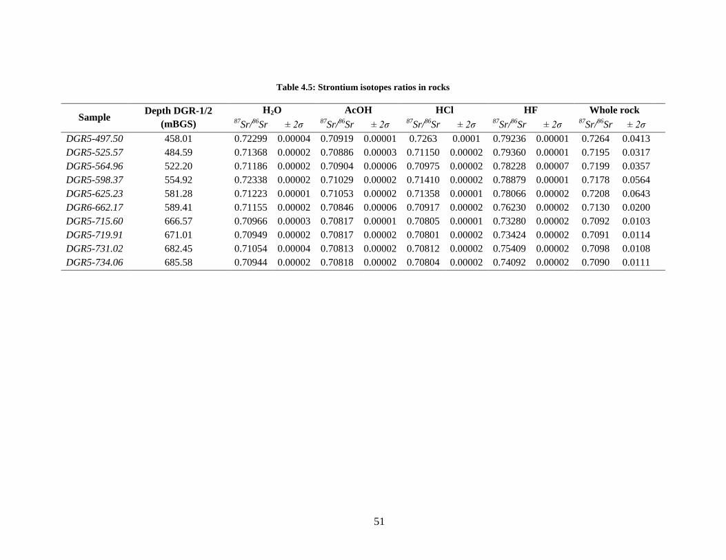
51
Table 4.5: Strontium isotopes ratios in rocks
Sample Depth DGR-1/2
(mBGS)
H2O AcOH HCl HF Whole rock 87
Sr/86
Sr ± 2σ 87
Sr/86
Sr ± 2σ 87
Sr/86
Sr ± 2σ 87
Sr/86
Sr ± 2σ 87
Sr/86
Sr ± 2σ
DGR5-497.50 458.01 0.72299 0.00004 0.70919 0.00001 0.7263 0.0001 0.79236 0.00001 0.7264 0.0413
DGR5-525.57 484.59 0.71368 0.00002 0.70886 0.00003 0.71150 0.00002 0.79360 0.00001 0.7195 0.0317
DGR5-564.96 522.20 0.71186 0.00002 0.70904 0.00006 0.70975 0.00002 0.78228 0.00007 0.7199 0.0357
DGR5-598.37 554.92 0.72338 0.00002 0.71029 0.00002 0.71410 0.00002 0.78879 0.00001 0.7178 0.0564
DGR5-625.23 581.28 0.71223 0.00001 0.71053 0.00002 0.71358 0.00001 0.78066 0.00002 0.7208 0.0643
DGR6-662.17 589.41 0.71155 0.00002 0.70846 0.00006 0.70917 0.00002 0.76230 0.00002 0.7130 0.0200
DGR5-715.60 666.57 0.70966 0.00003 0.70817 0.00001 0.70805 0.00001 0.73280 0.00002 0.7092 0.0103
DGR5-719.91 671.01 0.70949 0.00002 0.70817 0.00002 0.70801 0.00002 0.73424 0.00002 0.7091 0.0114
DGR5-731.02 682.45 0.71054 0.00004 0.70813 0.00002 0.70812 0.00002 0.75409 0.00002 0.7098 0.0108
DGR5-734.06 685.58 0.70944 0.00002 0.70818 0.00002 0.70804 0.00002 0.74092 0.00002 0.7090 0.0111

52
It is already known that limestones were precipitated from the seawater. Thus, it is
expected that the strontium isotope signatures of the carbonates (from the acetic acid and
hydrochloric acid leachates) to be the same than that of the seawater at the time of
deposition. As for the shales (DGR5-497.50 to DGR6-662.17) containing less carbonates,
they were not formed the same way than the Ordovician limestones, thus it would be
surprising that the associated AcOH and HCl leachates show the seawater values
(Spencer, 2013). The HF/HNO3 solutions, on the other hand, were expected to have very
high ratios, as they are rich in clays, thus concentrated in rubidium and have a high
potential for 87
Sr enrichment. Measured values for strontium isotopes ratios are consistent
with what was expected, based on rubidium contents. More explanations on the values
will be found in the next section, along with porewater values.
4.3.2 Porewaters
Strontium isotope ratios in porewaters are presented in Table 4.6. The first
observation is that ratios in porewaters show relatively constant values, slightly
increasing with depth, which is consistent with the initial observation made in 2011 (ref.
Figure 1.1).

53
Table 4.6: Strontium isotopes in porewaters
Sample
Depth
DGR-1/2
(mBGS)
87Sr/
86Sr ± 2σ
DGR5-497.50 458.01 0.70965 0.00005
DGR5-514.22 473.82 0.70964 0.00003
DGR5-525.57 484.59 0.70970 0.00002
DGR5-557.65 515.12 0.70971 0.00003
DGR5-564.96 522.20 0.70983 0.00002
DGR5-598.37 554.92 0.70988 0.00002
DGR5-625.23 581.28 0.70990 0.00002
DGR6-654.12 582.42 0.70992 0.00002
DGR6-661.83 589.11 0.70991 0.00002
DGR6-662.17 589.41 0.70987 0.00003
DGR6-662.82 589.98 0.70991 0.00003
DGR5-649.57 605.17 0.70993 0.00002
DGR6-683.25 607.67 0.70992 0.00003
DGR6-697.97 619.36 0.70989 0.00002
DGR5-671.30 625.33 0.70992 0.00002
DGR5-683.57 636.57 0.70994 0.00003
DGR5-697.85 649.71 0.70993 0.00003
DGR5-715.60 666.57 0.70988 0.00001
DGR5-724.60 676.15 0.70996 0.00002
DGR5-731.02 682.45 0.70989 0.00002
DGR5-734.06 685.58 0.70997 0.00003
Strontium isotope ratios of porewaters and of each leachate of rocks and are
plotted in Figure 4.6 along with ratios of seawater from the Ordovician and Silurian
(Veizer J. , 1989). Results will be discussed in the following section.
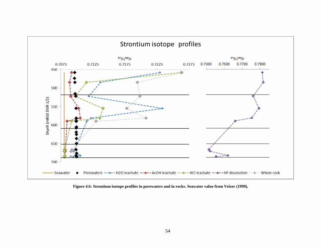
54
Figure 4.6: Strontium isotope profiles in porewaters and in rocks. Seawater value from Veizer (1999).

55
4.4 Dynamics
4.4.1 Equilibrium between rocks and porewaters
The first observation from Figure 4.6 is that strontium signatures of porewaters
are in total discordance with any phase of the rock, suggesting leaching of rocks by pore
fluids is very unlikely. In that case, strontium signatures in porewaters would have
reflected that of the rock, or at least one of the phases, since they would have reached
equilibrium over time. Moreover, concentrations of radiogenic strontium should be
directly derived from concentrations of radioactive rubidium. Thus, if clays were to
exclude radiogenic strontium in porewaters when it is formed, the isotopic ratio of
strontium in porewaters would reflect the trends of rubidium in clays. Figure 4.5 and
Figure 4.6, show that it is not the case, thus this hypothesis has to be rejected.
Another interesting observation can be made when comparing Figure 4.5 and
Figure 4.6. In the three first leachates, strontium isotopes ratios follow approximately the
same trend as rubidium-87 concentrations. The HF/HNO3 curve for 87
Rb shows a
negative excursion at the Queenston depths (518-609 m) while strontium isotopes are
going the other way. That could be intriguing at first sight, but a few calculations are
enough to prove it is still consistent. Using isotopes and concentrations of both elements,
it is possible to calculate the potential strontium isotopes ratio of a sample after a given
amount of time. Exhaustive calculations are shown in Appendix B. When applying these
calculations to each phase of the rock, using 0.7080 as initial ratio, the potential final
87Sr/
86Sr ratio is calculated. It is then possible to compare it to measurements in each
leachate. Calculations were performed using 450 million years (estimated time elapsed
since deposition) for H2O, AcOH and HCl leachates, and 415 million years for the HF

56
solution, since illites likely formed after the infiltration of the Silurian brine. Figure 4.7
shows profiles for measured ratios (dashed lines) along with calculated final ratios (solid
lines).
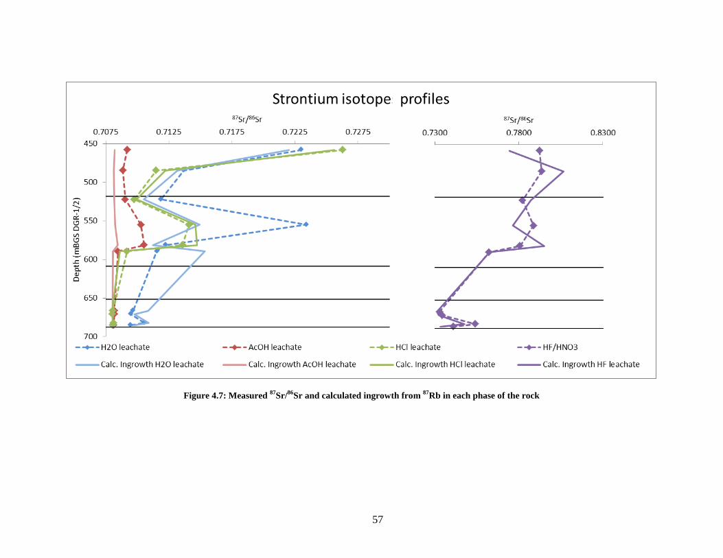
57
Figure 4.7: Measured 87
Sr/86
Sr and calculated ingrowth from 87
Rb in each phase of the rock

58
Although 87
Rb in for the HF curve was not consistent with measured strontium
isotopes in Figure 4.5, when considering the original amount of 87
Sr in samples, it is still
possible to get approximately to the measured values.
Hydrochloric acid leachates have strontium isotopes signatures very similar to what
would be expected with calculated ingrowths, suggesting this phase has not been exchanging
any rubidium or strontium since it has been formed. On the other hand, acetic acid leachates
seem to contain too little rubidium to decay to the measured strontium isotopes values. When
Silurian brines have infiltrated the Ordovician depths, they caused dolomitization that
changed strontium isotopic ratios, since the brine was richer in radiogenic strontium (up to
0.7088 during the Silurian) (ref. Figure 2.6).
2CaCO3 calcite + Mg2+
↔ CaMg(CO3)2 dolomite + Ca2+
CaCO3 calcite + Sr2+
↔ SrCO3 strontianite + Ca2+
Strontium in those brines had an enriched value of 87
Sr/86
Sr compared to calcite,
resulting in the formation (to trace levels) of enriched strontianite. When leaching those
rocks with acetic acid, strontianite dissolved (Bolton, 1878), causing the measured value of
87Sr/
86Sr to be higher than expected.
4.4.2 Ingrowth from groundwater
It is proven that the ingrowth of 87
Sr in porewaters cannot be attributed to leaching of
rocks or 87
Sr exclusion. That leaves only one other possibility: ingrowth of 87
Sr in the caused
by the 87
Rb decay in the porewaters themselves. In that case, the original strontium isotopes
ratios of porewaters have to be determined. Geochemical analysis showed porewaters likely
originated from a mixture of both Guelph and Cambrian groundwater, but another option is

59
that they find their origin in seawater trapped in pores when rocks formed. Both possibilities
have to be considered.
When taking concentrations of both rubidium and strontium, combined with isotopes
of both elements in porewaters, it is possible to calculate the original 87
Sr/86
Sr in porewaters
415 000 000 years ago (estimated age of the Silurian brine). However, this calculation will
be valid only in the case where no external sources of rubidium or strontium mixed with the
porewater, and where none of the elements precipitated or were lost by any process.
Exhaustive calculations are found in Appendix C.
Figure 4.8 represents measured strontium isotopes ratios for porewaters (black
diamonds), as well as those from both Guelph and Cambrian groundwaters (light blue
dashed line) (Heagle & Pinder, 2009). Guelph groundwater has undergone 87
Rb decay over
time as well; its value is represented (dark blue dot). For the Cambrian groundwater, Raven
et al. (2011) raised the possibility that radiogenic 87
Sr/86
Sr observed in the Middle
Ordovician limestones porewaters comes from the underlying Precambrian rocks. Enriched
brines from the Precambrian were measured in Sudbury (McNutt, Frape, & Fritz, 1984).
Movement of strontium into the overlying rocks, probably mixing with the Guelph
groundwater, is consistent with observations of other parameters such as δD and δ18
O
(Raven, et al., 2011). As a result, the original value for the Cambrian groundwater was set to
0.71035, which represents the average between the Precambrian brines and the original
Cambrian groundwater values. The resulting mixing line between the original Guelph and
Cambrian groundwaters is plotted (dark blue line). The graph also shows back-calculated
original ratios of porewaters (green stars) as well as the calculated ingrowth of radiogenic
strontium by 87
Rb decay in porewaters (red diamonds).

60
Figure 4.8: Original 87
Sr/86
Sr of porewaters and calculated ingrowth
The calculated original ratios show a strong correlation with the groundwaters mixing
line. This observation adds to the proof that porewaters originate from the infiltrated Guelph
groundwater and the diffusion of the Cambrian groundwater, likely mixed with Precambrian
brines. The calculated values for the ingrowth of 87
Sr in porewaters (Appendix C) are also
consistent with measurements, with very little variation. These calculations were performed
with the original groundwater values (dark blue line).
350
450
550
650
750
850
0,7090 0,7092 0,7094 0,7096 0,7098 0,7100 0,7102 0,7104D
epth
(m
BG
S D
GR
-1/2
)
87Sr/86Sr
Porewaters Groundwater mixing line today
Calculated original ratio Calculated ingrowth from groundwaters
Groundwater value, 415 my ago
61
4.4.3 Ingrowth from seawater
Constant strontium isotopes ratios in porewaters could lead thinking that they
originate from seawater trapped in pores when rocks were formed, and that 87
Sr has been
ingrowing overtime. The main difference between this scenario and the previous one is the
original strontium isotopes ratio of the water. In section 4.4.2, the original value was the mix
of both groundwaters. Here, it is the seawater ratio, 0.7080 (ref. Figure 2.6). Calculations
from the previous section were performed again considering this different parameter. Results
are plotted in Figure 4.9 (black line).
Furthermore, 87
Rb content in rocks was used to calculate the potential ingrowth of
strontium in the case that 87
Sr were to be expelled in porewaters once formed in minerals.
Although it is already demonstrated that this process does not take place in the system, this
consideration now adds to the proof that leaching from the rocks does not occur. For each
sample of porewater, the original amount of 87
Sr was added to the 87
Sr formed by 87
Rb decay
in porewaters and to the entire amount of 87
Sr formed by 87
Rb decay in each phase of the
matching rock sample. Full calculations are shown in Appendix D, and results are shown in
Figure 4.9. Calculations were performed for each phase of the rock, as well as for the whole
rock, considering 450 000 000 years (estimated time elapsed since deposition).

62
Figure 4.9: Calculated strontium isotopes ratios in porewaters, considering 450 000 000 years for 87
Rb decay
450
500
550
600
650
700
0,7075 0,7080 0,7085 0,7090 0,7095 0,7100 0,7105 0,7110 0,7115
Dep
th (
mB
GS
DG
R-1
/2)
87Sr/86Sr
Strontium isotopes profiles
Seawater Porewaters Ingrowth from porewaters H2O leachate
AcOH leachate HCl leachate HF leachate Whole rock

63
Figure 4.9 shows it would be impossible to reach the 87
Sr/86
Sr in porewaters when
considering their original ratio is that of the seawater (0.7080)., even when releasing
100% of the decayed rubidium (in 450 m.y.) from the rock into the porewaters. With the
exception of the two uppermost Queenston samples, the value is still far from the
measured ratio in most samples. Thus, the hypothesis suggesting the porewaters originate
from infiltrated and diffused groundwater remains the most plausible.
4.4.4 Strontium and Rubidium isotopes as a dating tool
One of the major problems when using the Rb-Sr method to date rocks is that
calculated ages are those of the formation of the rock, which is not necessarily the same
as its deposition. For sedimentary rocks, this rests on the assumption that all phases of the
rock were formed at the same time and were not transported, that strontium isotopes were
homogenized within the rock during its formation, and that the system remained close
until today. In the case of the studied Ordovician shales and limestones, isochrons were
traced and interpreted to have a better understanding of the interactions.
Isochrons were plotted for each leachate (Figure 4.10), with measured strontium
isotopes ratios and with calculated ingrown 87
Sr from 87
Rb. A time of 450 million years
was used in calculations for H2O, AcOH and HCl leachates, and 415 million years was
used for HF/HNO3 dissolution, as illites likely formed with the Silurian brines (see
calculations in Appendix B). Table 4.7 shows, for each isochron, the value of the slope,
intercept, determination coefficient (r2) as well as the calculated age obtained from those
parameters.

64
Figure 4.10: Isochrons for A) Water leachate, B) Acetic acid leachate, C) Hydrochloric acid leachate, D) Hydrofluoric acid dissolution.
0,7050
0,7100
0,7150
0,7200
0,7250
0,0 0,5 1,0 1,5 2,0 2,5
87 S
r/8
6 Sr
87Rb/86Sr
H2O leachate
Measured ratios Calculated ingrowth (450 m.y.)
0,7070
0,7080
0,7090
0,7100
0,7110
0,00 0,02 0,04 0,06 0,08
87 S
r/8
6 Sr
87Rb/86Sr
AcOH leachate
Measured ratios Calculated ingrowth (450 m.y.)
0,7050
0,7100
0,7150
0,7200
0,7250
0,7300
0,0 0,5 1,0 1,5 2,0 2,5 3,0 3,5
87 S
r/8
6 Sr
87Rb/86Sr
HCl leachate
Measured ratios Calculated ingrowth (450 m.y.)
0,7200
0,7400
0,7600
0,7800
0,8000
0,8200
0 5 10 15 20
87 S
r/8
6 Sr
87Rb/86Sr
HF/HNO3 dissolution
Measured ratios Calculated ingrowth (415 m.y.)
B)
C) D)
A)

65
Table 4.7: Statistical parameters and calculated age for each isochron
Leach Slope Intercept r2 Calculated age (years)
H2O 0.0071 0.7079 0.6625 509 300 000 ± 128 000 000
AcOH 0.0369 0.7081 0.9123 2 779 300 000 ± 298 900 000
HCl 0.0064 0.7078 0.9902 453 700 000 ± 15 900 000
HF/HNO3 0.0048 0.7198 0.8613 339 700 000 ± 48 000 000
In the first three isochron, values of intercepts reflect that of the seawater
(0.7080), with minor differences. That is consistent with the fact that rocks dissolved in
those three leachates are mostly evaporites and carbonates, deposited from marine
environments. Values for the water leachate isochron do not show a very strong
correlation (r2=0.6625), mostly because this leachate did not target any mineral
specifically. Celestite have probably dissolved at this step (Reardon & Armstrong, 1987),
with a few other evaporites and adsorbed ions. As a result, a trend is observable, the
calculated age is consistent, but the correlation is weak.
The acetic acid isochon is also consistent with Figure 4.7 where it was shown that
calcite does not contain enough rubidium to get to the measured strontium isotopes ratios.
However, the isochron shows a strong correlation between the ratios and 87
Rb/86
Sr,
suggesting not only calcite was dissolved by acetic acid. Strontianite, formed along with
dolomite (see section 4.4.1) has probably dissolved at this step, enriching the 87
Sr/86
Sr in
leachates. As a result, the calculated age is not representative of reality. On the other
hand, the hydrochloric acid isochron, which represents dolomite, is exactly as expected.
Its calculated age of 453 700 000 years and its strong correlation (r2 = 0.9902) are
consistent with the estimated time of deposition for carbonates.

66
Finally, the HF/HNO3 isochron shows a significant correlation between the two
isotopes ratios. The calculated age of 339.7 million years corresponds to the age of
illitization, when the original smectites were converted to illite by uptake of K and Rb
from the infiltrating Silurian brine.
It is impossible to trace such isochrons for porewaters, since each sample has a
different 87
Sr/86
Sr original value from the mixing line. However, ages can be calculated
for each sample individually. Stable isotopes (D, 18
O, 3He,
13CH4, and
13CO2) provided
evidence for porewater residence time approaching the age of the rock (Al, Clark,
Kennell, Jensen, & Raven, 2014) (Clark, et al., 2013) (Clark, et al., 2013). They were also
used to prove the system remained close since the Silurian brine infiltration. All
conditions being met to date pore fluids, estimations of their age were obtained by
calculating the difference between the estimated original mixing line and the measured
values (ref. Figure 4.8). For each sample, the calculated age is reported in Table 4.8.

67
Table 4.8: Estimated ages of porewaters
Sample Depth (mBGS DGR-1/2) Calculated age (years)
DGR5-497.50 458.01 621 600 000 ± 58 500 000
DGR5-514.22 473.82 445 900 000 ± 34 300 000
DGR5-525.57 484.59 553 800 000 ± 34 100 000
DGR5-557.65 515.12 425 700 000 ± 37 100 000
DGR5-564.96 522.20 705 400 000 ± 40 500 000
DGR5-598.37 554.92 397 000 000 ± 22 700 000
DGR5-625.23 581.28 452 100 000 ± 31 900 000
DGR6-654.12 582.42 599 900 000 ± 35 500 000
DGR6-661.83 589.11 581 900 000 ± 35 500 000
DGR6-662.17 589.41 559 500 000 ± 59 600 000
DGR6-662.82 589.98 571 400 000 ± 45 500 000
DGR5-649.57 605.17 536 900 000 ± 43 700 000
DGR6-683.25 607.67 481 700 000 ± 42 800 000
DGR6-697.97 619.36 406 000 000 ± 38 600 000
DGR5-671.30 625.33 454 000 000 ± 39 400 000
DGR5-683.57 636.57 425 700 000 ± 54 300 000
DGR5-697.85 649.71 297 200 000 ± 44 300 000
DGR5-715.60 666.57 200 200 000 ± 79 600 000
DGR5-724.60 676.15 713 400 000 ± 144 600 000
DGR5-731.02 682.45 (34 000 000)1
± 67 800 000
DGR5-734.06 685.58 280 200 000 ± 68 700 000 1Measured
87Sr/
86Sr is smaller than the original estimated value by the mixing line. See Figure 4.8.
Samples from the shales (DGR5-497.50 to DGR5-697.85) show ages fairly
consistent with the Ordovician. Variations and large uncertainties are attributed to the
approximation of the original 87
Sr/86
Sr values by the mixing line between both
groundwaters (ref. Figure 4.8), and to the fact that rubidium is exchanging with clays at
an unknown rate. As for limestones (DGR5-715.60 to DGR5-734.06), their estimated age
is much lower than reality. This could be attributed to their very low concentration in
rubidium, but also to the difficulty setting a value of 87
Sr/86
Sr in the Cambrian
groundwater, as the exchange rate between this water and the Precambrian brines is
undetermined.

68
5.0 CONCLUSIONS
This study shows that the use of geochemistry, combined with rubidium and
strontium isotopes, can help understanding the dynamics between rocks and pore fluids.
These methods were used to complete the three primary objectives of this thesis, which
were (1) to determine the origin of porewaters, (2) to explain the difference in strontium
isotopes ratios between the host rocks and their porewaters, and (3) to estimate ages of
both rocks and porewaters in the Ordovician shales and limestones, at the DGR site, in
Kincardine, Ontario.
5.1 Origin of porewaters
When calculating the original 87
Sr/86
Sr ratio from the measured ratios in
porewaters, values corresponding to a mixing line between the Guelph and Cambrian
groundwaters were obtained. This suggests porewaters are the result of a mix between the
overlying Silurian brines that infiltrated the system, and upward diffusion of the
Cambrian groundwaters, likely mixed with Precambrian brined to some extent. This
explanation is consistent with other observations from this site (Raven, et al., 2011).
The Ordovician seawater has an 87
Sr/86
Sr of 0.7080. Starting with this original
amount of 87
Sr, it is impossible to reach the measured values of 87
Sr/86
Sr when taking
87Rb decay into account.
5.2 Ingrowth of 87
Sr
Isotopes of both elements showed that the ingrowth of radiogenic strontium in
porewaters cannot be caused by pore fluids leaching rocks, as their isotope ratios would
have equilibrated over time. Also, it is very unlikely that radiogenic strontium, once

69
formed by 87
Rb decay, is expelled from minerals and transferred into porewaters. In that
case, 87
Rb in rocks and 87
Sr/86
Sr in porewaters would follow the same trends. The
ingrowth of 87
Sr was thus attributed to the 87
Rb decay in porewaters themselves.
Calculations support this explanation.
5.3 Rb-Sr dating
Ages were estimated for pore fluids and isochrones were traced for each phase of
the rocks using strontium and rubidium isotopes. The hydrochloric acid leachates, mostly
containing dolomites, gave a reliable age (453 700 000 years before present)
corresponding to that of their deposition. The HF/HNO3 isochron gave an age that could
correspond to that of illitization, as the process took place after rocks were deposited. The
estimated age is 339.7 million years.
5.4 Recommendations
Should additional investigations be conducted to evaluate the age of rocks or
porewaters, it is recommended that other isotopes systems be used to compare results.
Analyses of other isotopes systems could also add to the understanding of the water-rock
interaction at this site.
Furthermore, additional investigations on clays are suggested to differentiate ions
and isotopes from the interlayers than those from their structures. This could provide
clues on their real age of formation and how they interacted with the pore fluids and other
phases of rocks.
On a technical level, it is suggested to conduct extensive analyses to determine the
best conditions required to dissolve each mineral during the leaching sequence. Different

70
times of reaction, temperatures, and many more chemicals could be tried to dissolve
various minerals. Moreover, analyses of the remaining rocks after each leach should be
conducted to determine what minerals were dissolved in each leachate.

71
REFERENCES
Al, T., Clark, I. D., Kennell, L., Jensen, M., & Raven, K. (2014). Geochemical Evolution
and Residence Time of Porewater in Low-Permeability Rocks of the Michigan
Basin, Southwest Ontario. Unpublished.
Anderson, D. L. (1989). Theory of the Earth. Boston: Blackwell Scientific Publications.
Armstrong, D. K., & Carter, T. R. (2010). The Subsurface Paleozoic Stratigraphy of
Southern Ontario. Ontario Geological Survey, Special Volume 7.
Bailey, T. R., McArthur, J. M., Prince, H., & Thirlwall, M. F. (2000). Dissolution
methods for strontium isotope stratigraphy: whole rock analysis. Chemical
Geology, 167, 313-319.
Bofinger, V. M., Compston, W., & Vernon, M. J. (1968). The application of acid
leaching ot the Rb-Sr dating of a Middle Ordovician shale. Geochimica et
Cosmochimica Acta, 32, 823-833.
Bolton, H. C. (1878). Application of organic acids to the examination of minerals. (W.
Crookes, Ed.) The Chemical News and Journal of Industrial Science, 37(951), 65-
67.
Burke, W. H., Denison, R. E., Hetherington, E. A., Koepnick, R. B., Nelson, H. F., &
Otto, J. B. (1982). Variation of seawater 87Sr/86Sr through Phanezoroic time.
Geology, 10, 516-519.
Capo, R. C., Stewart, B. W., & Chadwick, O. A. (1998). Strontium isotopes as tracers of
ecosystem processes: theory and methods. Geoderma, 82(1-3), 197-225.
Carleton University. (2012). Isotope Geochemistry and Geochronology Research Centre.
Retrieved 09 11, 2014, from Isotope Geochemistry and Geochronology Research
Centre: http://iggrc.carleton.ca/
Chaudhuri, S., & Brookins, D. G. (1969). The Rb-Sr Whole-Rock Age od the Stearns
Shale (Lower Permian), Eastern Kansas, before and after Acid Leaching
Experiments. Geological Society of America Bulletin, 80, 2605-2610.
72
Chaudhuri, S., & Clauer, N. (1992). History of Marine Evaporites : Constraints from
Radiogenic Isotopes. (N. Clauer , & S. Chaudhuri, Eds.) Lecture Notes in Earth
Sciences, 43, 177-198.
Clark, I. D., Al, T., Jensen, M., Kennell, L., Mazurek, M., Mohapatra, R., & Raven, K.
(2013). Paleozoic-aged brine and authigenic helium preserved in an Ordovician
shale aquiclude. Geological Society of America, 41(9), 951-954.
Clark, I. D., Ilin, D., Jackson, R., Jensen, M., Kennell, L., Mohammadzadeh, H., . . .
Xing, Y. (2013). Microbial methane of Paleozoic age preserved in Ordovician
shales od the Michigan basin, Kincardine, Ontario. Unpublished.
Clark, I., & Fritz, P. (1997). Environmental Isotopes in Hydrogeology. Boca Raton,
Florida: CRC Press.
Clark, I., Scharf, V., Zuliani, J., & Herod, M. (2011). Porewater Analyses in DGR-5 and
DGR-6 Core, Technical Report TR-09-07. DGR Site Characterization Document,
Geofirma Engineering, Toronto.
Clauer, N., Chaudhuri, S., Kralik, M., & Bonnot-Courtois, C. (1993). Effects of
experimental leaching on Rb-Sr and K-Ar isotopic systems and REE contents of
diagenetic illite. Chemical Geology, 103, 1-16.
de Laeter, J. R., Böhlke, J. K., De Bièvre, P., Hidaka, H., Peiser, H. S., Rosman, K. J., &
Taylor, P. D. (2003). Atomic weights of the elements. Review 2000 (IUPAC
Technical Report). Pure and Applied Chemistry, 75(6), 683-800.
Donaldson, W. S. (1989). The depositional environment of the Queenston Shale,
southwestern Ontario. Proceedings, Ontario Petroleum Institute, 28th annual
conference, 28, Technical Paper 16. London, Ontario.
Faure, & Gunter. (1991). Principles and applications of inorganic geochemistry: A
comprehensive textbook for geology students. New York, NY: Macmillan
Publication Co.
Faure, G. (1986). Principles of Isotope Geology. New York, NY: Wiley.
73
Frape, S. K., Fritz, P., & McNutt, R. H. (1984). The role of water-rock interaction in the
chemical evolution of groundwaters from the Canadian Shiels. Geochimica et
Cosmochimica Acta, 48, 1617-1627.
Ganguly, A. (2012). Fundamentals of Inorganic Chemistry (2nd ed.). New Delhi, India:
Pearson.
Google Maps. (2014). Google Maps. Retrieved Jan 15, 2014, from Google Maps:
http://maps.google.ca
Gosselin, D. C., Harvey, F. H., Frost, C., Stotler, R., & Macfarlane, P. A. (2004).
Strontium isotope geochemistry of groundwater in the central part of the Dakota
(Great Plains) aquifer, USA. Applied Geochemistry, 19, 349-377.
Heagle, D., & Pinder, L. (2009). Opportunistic Groundwater Sampling in DGR-3 and
DGR-4, Technical Report TR-08-18. DGR Site Characterization Document, Intera
Engineering, Toronto.
Hodell, D. A., Mead, G. A., & Mueller, P. A. (1990). Variation in the strontium isotopic
composition of seawater (8 Ma to present) : Implications for chemical weathering
rates and dissolved fluxes to the oceans. Chemical Geology : Isotope Geoscience
section, 80, 291-307.
Holden, N. E. (2004). Section 11 : Table of the Isotopes. In W. M. (dir.), CRC Handbook
of Chemistry and Physics (85th ed.). Boca Raton, Florida: CRC Press.
Holland, H. D. (1984). The Chemical Evolution of the Atmospheres and Ocean.
Princeton, NJ: Princeton University.
Isotope Geochemistry and Geochronology Research Centre. (2013). Rb/Sr/REE
Extraction Procedure With Dowex 50-X8 Cation Resin. Carleton University.
Jackson, R., & Heagle, D. (2010). Opportunistic Groundwater Sampling in DGR-1 &
DGR-2, Technical Report TR-07-11. DGR Site Characterization Document, Intera
Engineering, Toronto.
Jackson, R., & Murphy, S. (2011). Mineralogical and Lithogeochemical Analyses of
DGR-5 and DGR-6 Core, Technical Report TR-09-06. 158.

74
Jacobson, A. D., Blum, J. D., Page Chamberlain, C., Poage, M. A., & Sloan, V. F.
(2002). Ca/Sr and Sr isotope systematics of a Himalayan glacial chronosequence :
Carbonate versus silicate weathering rates as a function of landscape surface age.
Geochimica et Cosmochimica Acta, 66(1), 13-27.
Kobluk, D. R., & Brookfield, M. E. (1982). Excursion 12A : Lower Paleozoic carbonate
rocks and paleoenvironments in southern Ontario. Field Excursion Guidebook.
Lerouge, C., Gaucher, E. C., Tournassat, C., Negrel, P., Crouzet, C., Guerrot, C., . . .
Buschaert, S. (2010). Strontium distribution and origins in a natural clayey
formation (Callovian-Oxfordian, Paris Basin, France): A new sequential
extraction procedure. Geochimica et Cosmochimica Acta, 74, 2926-2942.
Li, D., Shields-Zhou, G. A., Ling, H.-F., & Thirlwall, M. (2011). Dissolution methods for
strontium isotope stratigraphy: Guidelines for the use of bulk carbonate and
phosphorite rocks. Chemical Geology, 290, 133-144.
Lide, D. R. (2005). Section 14 : Geophysics, Astronomy, and Acoustics; Abundance of
Elements in the Earth's Crust and in the Sea. In W. M. Haynes, CRC Handbook of
Chemistry and Physics (85th ed.). Boca Raton, Florida: CRC Press.
Macauley, G., Fowler, M. G., Goodarzi, F., Snowdon, L. R., & Stasiuk, L. D. (1990).
Ordovician oil shale-source rock sediments in the central and eastern Canada
mainland and eastern arctic areas, and their significance for frontier exploration.
Geological Survey of Canada, Paper 90-14.
McNutt, R. H., Frape, S. K., & Fritz, P. (1984). Strontium isotopic composition of some
brines from the Precambrian Shield of Canada. Isotope Geoscience, 2, 205-215.
National Aeronautics and Space Administration. (2012). WMAP - Age of the Universe.
Retrieved Februrary 19, 2014, from National Aeronautics and Space
Administration: http://map.gsfc.nasa.gov/universe/uni_age.html
Nelson, S. A. (2013). Radiometric Dating. Retrieved 02 19, 2014, from Tulane
University, Earth & Environmental Sciences 2110, Mineralogy:
http://www.tulane.edu/~sanelson/eens211/radiometric_dating.htm

75
Papanastassiou, D. A., Wasserburg, G. J., & Burnett, D. S. (1969). Initial strontium
isotopic abundances and the resolution of small time differences in the formation
of planetary objects. Earth Planetary Science Letters, 5, 361-76.
Patchett, P. J., & Samson, S. D. (2003). Ages and growth of the continental crust from
radiogenic isotopes. (H. D. Holland, & K. K. Turekian, Eds.) Treatise on
Geochemistry, 3, 321-348.
Raven, K., McCreath, D., Jackson, R., Clark, I., Heagle, D., Sterling, S., & Melaney, M.
(2011). OPG's Deep Geologic Repository for Low & Intermediate Level Waste :
Descriptive Geosphere Site Model, NWMO DGR-TR-2011-24. Intera Engineering
Ltd. & Nuclear Waste Management Organization, Toronto.
Reardon, E. J., & Armstrong, D. K. (1987). Celestite solubility in water, seawater and
NaCl solution. Geochimica et Cosmochimica Acta, 51(1), 63-72.
Rotenberg, E., Davis, D. W., Amelin, Y., Ghosh, S., & Bergquist, B. A. (2012).
Determination of the decay-constant of 87Rb by laboratory accumulation of 87Sr.
Geochimica et Cosmochimica Acta, 85(15), 41-57.
Shannon, R. D. (1976). Revised effective ionic radii and systematic studies of interatomic
distances in halides and chalcogenides. Acta Crystallographica Section A, A32,
751-67.
Sharp, M., Creaser, R. A., & Skidmore, M. (2002). Strontium isotope composition of
runoff from a glaciated carbonate terrain. Geochimica et Cosmochimica Acta,
66(4), 595-614.
Spencer, E. A. (2013). Personal communication, University of Ottawa.
Sposito, G. (1989). The Chemistry of Soils. New York, NY: Oxford Univ. Press.
Tessier, A., Campbell, P., & Bisson, M. (1979). Sequential Extraction Procedure for the
Speciation of Particulate Trace Metals. Analytical Chemistry, 51(7), 844-851.
Veizer, J. (1989). Strontium isotopes in seawater through time. Annual Review of Earth
and Planetary Science, 17, 141-167.
76
Veizer, J. (1992). Depositional and diagenetic History of Limestones : Stable and
Radiogenic Isotopes. (N. Clauer, & S. Chaudhuri, Eds.) Lecture Notes in Earth
Sciecnces, 43, 13-48.
Wilson, B. M. (1989). Igneous Petrogenesis : A Global Tectonic Approach (1st ed.).
Netherlands: Harper Collins Academic.

77
APPENDIX A:
SR EXTRACTION PROCEDURE WITH CATION RESIN
78
PROCEDURE
1. Remove parafilm and caps from orange columns, let columns drain.
2. Sample should have been dissolved overnight in 1.5 ml 2.5N HCl, preferably on a
90°C hotplate. Label centrifuge tubes and centrifuge samples for at least 4 minutes.
3. Add samples to columns with 0.5ml pipette, being careful to get drops to fall to the
top of the resin bed without touching the column walls. Do not let the pipette tip seal
against the top of the column, or you will create a vacuum in the column when you let
up on the pipette plunger.
4. Wash down the sides of the column with ~ 1 ml 2.5N HCl by twirling the column
with one hand and squirting acid in the top for a couple of seconds with the other.
5. Add 16ml 2.5ml HCl, let drain through.
6. Place clean, labelled snap-cap beaker under column, and discard acid in waste bucket.
Leave snap-cap lids on the carousel.
8. Add 6ml 2.5N HCl, collect in snap-cap beaker (the Sr fraction). When complete, put
on hot-plate to dry. Replace waste bucket under column.
CLEANING
Add 3 column volumes of 6N HCl; resin shrinks. Add one column volume of ~ 2N HCl,
resin epands. Add 8ml 2.5N HCl (half-way up the yellow buckets), resin equilibrates. Cut
parafilm to seal the base of the columns, add ~ 2mls 2.5N HCl to the columns to keep
them wet, and put the caps back on the top.
(Isotope Geochemistry and Geochronology Research Centre, 2013)
79
APPENDIX B:
CALCULATED 87
SR/86
SR INGROWTH IN ROCKS
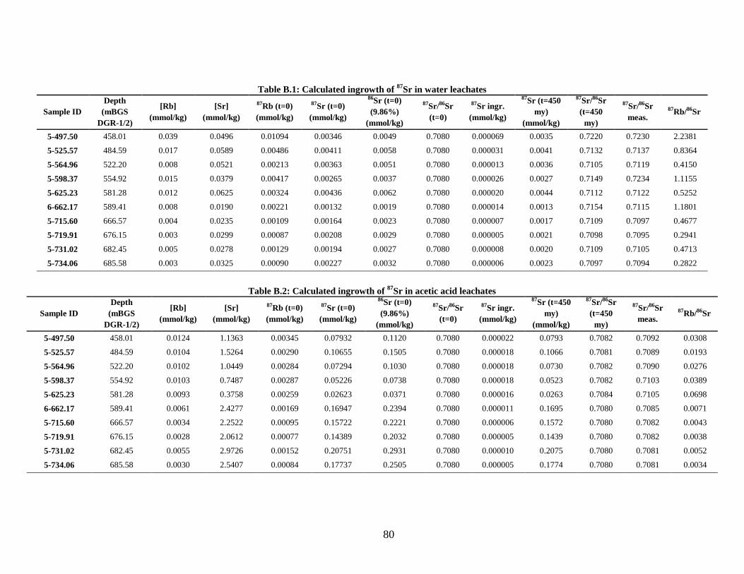
80
Table B.1: Calculated ingrowth of 87
Sr in water leachates
Sample ID
Depth
(mBGS
DGR-1/2)
[Rb]
(mmol/kg)
[Sr]
(mmol/kg)
87Rb (t=0)
(mmol/kg)
87Sr (t=0)
(mmol/kg)
86Sr (t=0)
(9.86%)
(mmol/kg)
87Sr/86Sr
(t=0)
87Sr ingr.
(mmol/kg)
87Sr (t=450
my)
(mmol/kg)
87Sr/86Sr
(t=450
my)
87Sr/86Sr
meas. 87Rb/86Sr
5-497.50 458.01 0.039 0.0496 0.01094 0.00346 0.0049 0.7080 0.000069 0.0035 0.7220 0.7230 2.2381
5-525.57 484.59 0.017 0.0589 0.00486 0.00411 0.0058 0.7080 0.000031 0.0041 0.7132 0.7137 0.8364
5-564.96 522.20 0.008 0.0521 0.00213 0.00363 0.0051 0.7080 0.000013 0.0036 0.7105 0.7119 0.4150
5-598.37 554.92 0.015 0.0379 0.00417 0.00265 0.0037 0.7080 0.000026 0.0027 0.7149 0.7234 1.1155
5-625.23 581.28 0.012 0.0625 0.00324 0.00436 0.0062 0.7080 0.000020 0.0044 0.7112 0.7122 0.5252
6-662.17 589.41 0.008 0.0190 0.00221 0.00132 0.0019 0.7080 0.000014 0.0013 0.7154 0.7115 1.1801
5-715.60 666.57 0.004 0.0235 0.00109 0.00164 0.0023 0.7080 0.000007 0.0017 0.7109 0.7097 0.4677
5-719.91 676.15 0.003 0.0299 0.00087 0.00208 0.0029 0.7080 0.000005 0.0021 0.7098 0.7095 0.2941
5-731.02 682.45 0.005 0.0278 0.00129 0.00194 0.0027 0.7080 0.000008 0.0020 0.7109 0.7105 0.4713
5-734.06 685.58 0.003 0.0325 0.00090 0.00227 0.0032 0.7080 0.000006 0.0023 0.7097 0.7094 0.2822
Table B.2: Calculated ingrowth of 87
Sr in acetic acid leachates
Sample ID
Depth
(mBGS
DGR-1/2)
[Rb]
(mmol/kg)
[Sr]
(mmol/kg)
87Rb (t=0)
(mmol/kg)
87Sr (t=0)
(mmol/kg)
86Sr (t=0)
(9.86%)
(mmol/kg)
87Sr/86Sr
(t=0)
87Sr ingr.
(mmol/kg)
87Sr (t=450
my)
(mmol/kg)
87Sr/86Sr
(t=450
my)
87Sr/86Sr
meas. 87Rb/86Sr
5-497.50 458.01 0.0124 1.1363 0.00345 0.07932 0.1120 0.7080 0.000022 0.0793 0.7082 0.7092 0.0308
5-525.57 484.59 0.0104 1.5264 0.00290 0.10655 0.1505 0.7080 0.000018 0.1066 0.7081 0.7089 0.0193
5-564.96 522.20 0.0102 1.0449 0.00284 0.07294 0.1030 0.7080 0.000018 0.0730 0.7082 0.7090 0.0276
5-598.37 554.92 0.0103 0.7487 0.00287 0.05226 0.0738 0.7080 0.000018 0.0523 0.7082 0.7103 0.0389
5-625.23 581.28 0.0093 0.3758 0.00259 0.02623 0.0371 0.7080 0.000016 0.0263 0.7084 0.7105 0.0698
6-662.17 589.41 0.0061 2.4277 0.00169 0.16947 0.2394 0.7080 0.000011 0.1695 0.7080 0.7085 0.0071
5-715.60 666.57 0.0034 2.2522 0.00095 0.15722 0.2221 0.7080 0.000006 0.1572 0.7080 0.7082 0.0043
5-719.91 676.15 0.0028 2.0612 0.00077 0.14389 0.2032 0.7080 0.000005 0.1439 0.7080 0.7082 0.0038
5-731.02 682.45 0.0055 2.9726 0.00152 0.20751 0.2931 0.7080 0.000010 0.2075 0.7080 0.7081 0.0052
5-734.06 685.58 0.0030 2.5407 0.00084 0.17737 0.2505 0.7080 0.000005 0.1774 0.7080 0.7081 0.0034
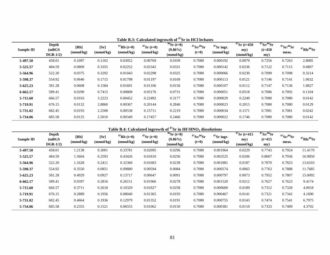
81
Table B.3: Calculated ingrowth of 87
Sr in HCl lechates
Sample ID
Depth
(mBGS
DGR-1/2)
[Rb]
(mmol/kg)
[Sr]
(mmol/kg)
87Rb (t=0)
(mmol/kg)
87Sr (t=0)
(mmol/kg)
86Sr (t=0)
(9.86%)
(mmol/kg)
87Sr/86Sr
(t=0)
87Sr ingr.
(mmol/kg)
87Sr (t=450
my)
(mmol/kg)
87Sr/86Sr
(t=450
my)
87Sr/86Sr
meas. 87Rb/86Sr
5-497.50 458.01 0.1097 0.1102 0.03052 0.00769 0.0109 0.7080 0.000192 0.0079 0.7256 0.7263 2.8085
5-525.57 484.59 0.0809 0.3355 0.02252 0.02342 0.0331 0.7080 0.000142 0.0236 0.7122 0.7115 0.6807
5-564.96 522.20 0.0375 0.3292 0.01043 0.02298 0.0325 0.7080 0.000066 0.0230 0.7099 0.7098 0.3214
5-598.37 554.92 0.0646 0.1715 0.01798 0.01197 0.0169 0.7080 0.000113 0.0121 0.7146 0.7141 1.0632
5-625.23 581.28 0.0608 0.1584 0.01691 0.01106 0.0156 0.7080 0.000107 0.0112 0.7147 0.7136 1.0827
6-662.17 589.41 0.0290 0.7415 0.00808 0.05176 0.0731 0.7080 0.000051 0.0518 0.7086 0.7092 0.1104
5-715.60 666.57 0.0163 3.2223 0.00452 0.22492 0.3177 0.7080 0.000029 0.2249 0.7080 0.7080 0.0142
5-719.91 676.15 0.0132 2.8860 0.00367 0.20144 0.2846 0.7080 0.000023 0.2015 0.7080 0.7080 0.0129
5-731.02 682.45 0.0193 2.2508 0.00538 0.15711 0.2219 0.7080 0.000034 0.1571 0.7081 0.7081 0.0242
5-734.06 685.58 0.0125 2.5010 0.00349 0.17457 0.2466 0.7080 0.000022 0.1746 0.7080 0.7080 0.0142
Table B.4: Calculated ingrowth of 87
Sr in HF/HNO3 dissolutions
Sample ID
Depth
(mBGS
DGR-1/2)
[Rb]
(mmol/kg)
[Sr]
(mmol/kg)
87Rb (t=0)
(mmol/kg)
87Sr (t=0)
(mmol/kg)
86Sr (t=0)
(9.86%)
(mmol/kg)
87Sr/86Sr
(t=0)
87Sr ingr.
(mmol/kg)
87Sr (t=415
my)
(mmol/kg)
87Sr/86Sr
(t=415
my)
87Sr/86Sr
meas. 87Rb/86Sr
5-497.50 458.01 1.2138 0.3001 0.33781 0.02095 0.0296 0.7080 0.001964 0.0229 0.7743 0.7924 11.4170
5-525.57 484.59 1.5604 0.2593 0.43426 0.01810 0.0256 0.7080 0.002525 0.0206 0.8067 0.7936 16.9850
5-564.96 522.20 1.1628 0.2411 0.32360 0.01683 0.0238 0.7080 0.001881 0.0187 0.7870 0.7823 13.6103
5-598.37 554.92 0.3550 0.0851 0.09880 0.00594 0.0084 0.7080 0.000574 0.0065 0.7763 0.7888 11.7685
5-625.23 581.28 0.4929 0.0927 0.13717 0.00647 0.0091 0.7080 0.000797 0.0073 0.7952 0.7807 15.0092
6-662.17 589.41 0.9397 0.2816 0.26151 0.01966 0.0278 0.7080 0.001520 0.0212 0.7627 0.7623 9.4174
5-715.60 666.57 0.3711 0.2618 0.10329 0.01827 0.0258 0.7080 0.000600 0.0189 0.7312 0.7328 4.0018
5-719.91 676.15 0.2889 0.1956 0.08040 0.01365 0.0193 0.7080 0.000467 0.0141 0.7321 0.7342 4.1690
5-731.02 682.45 0.4664 0.1936 0.12979 0.01352 0.0191 0.7080 0.000755 0.0143 0.7474 0.7541 6.7975
5-734.06 685.58 0.2355 0.1521 0.06555 0.01062 0.0150 0.7080 0.000381 0.0110 0.7333 0.7409 4.3702

82
APPENDIX C:
87SR/
86SR INGROWTH FROM GROUNDWATERS

83
Table C.1: Calculated original 87
Sr/86
Sr values for porewaters
Sample ID [Rb]
(mmol/kg)
[Sr]
(mmol/kg)
87Rb (t=x)
(mmol/kg)
87Sr (t=x)
(mmol/kg)
86Sr
(9.86%)
(mmol/kg)
87Sr/86Sr
meas.
87Sr ingrown
(t=415 my)
(mmol/kg)
87Rb (t=0)
(mmol/kg)
87Sr (t=0)
(mmol/kg)
87Sr/86Sr
(t=0)
DGR5-497.50 0.1973 12.5879 0.0549 0.8808 1.2412 0.7097 0.000319 0.0552 0.8805 0.7094
DGR 5-514.22 0.2204 11.8418 0.0613 0.8286 1.1676 0.7096 0.000357 0.0617 0.8282 0.7093
DGR 5-525.57 0.2259 13.8559 0.0629 0.9696 1.3662 0.7097 0.000365 0.0632 0.9692 0.7094
DGR 5-557.65 0.1988 11.7838 0.0553 0.8246 1.1619 0.7097 0.000322 0.0556 0.8243 0.7094
DGR 5-564.96 0.2399 17.4436 0.0668 1.2209 1.7199 0.7098 0.000388 0.0672 1.2205 0.7096
DGR 5-598.37 0.2511 11.4331 0.0699 0.8003 1.1273 0.7099 0.000406 0.0703 0.7999 0.7095
DGR 5-625.23 0.2025 12.7742 0.0563 0.8941 1.2595 0.7099 0.000328 0.0567 0.8938 0.7096
DGR 6-654.12 0.2214 17.6451 0.0616 1.2351 1.7398 0.7099 0.000358 0.0620 1.2348 0.7097
DGR 6-661.83 0.1974 16.8220 0.0549 1.1775 1.6587 0.7099 0.000319 0.0552 1.1772 0.7097
DGR 6-662.17 0.2011 19.4805 0.0560 1.3635 1.9208 0.7099 0.000325 0.0563 1.3632 0.7097
DGR 6-662.82 0.1914 16.0861 0.0533 1.1260 1.5861 0.7099 0.000310 0.0536 1.1257 0.7097
DGR 5-649.57 0.1634 14.2253 0.0455 0.9958 1.4026 0.7099 0.000264 0.0457 0.9955 0.7097
DGR 6-683.25 0.1802 14.6662 0.0501 1.0266 1.4461 0.7099 0.000291 0.0504 1.0263 0.7097
DGR 6-697.97 0.2084 19.5379 0.0580 1.3676 1.9264 0.7099 0.000337 0.0583 1.3672 0.7097
DGR 5-671.30 0.1430 13.9241 0.0398 0.9747 1.3729 0.7099 0.000231 0.0400 0.9744 0.7098
DGR 5-683.57 0.1915 19.5373 0.0533 1.3676 1.9264 0.7099 0.000310 0.0536 1.3673 0.7098
DGR 5-697.85 0.1696 17.0141 0.0472 1.1910 1.6776 0.7099 0.000274 0.0475 1.1907 0.7098
DGR 5-715.60 0.0591 19.4800 0.0164 1.3635 1.9207 0.7099 0.000096 0.0165 1.3634 0.7098
DGR 5-724.60 0.0543 20.0800 0.0151 1.4056 1.9799 0.7100 0.000088 0.0152 1.4056 0.7099
DGR 5-731.02 0.0550 11.1500 0.0153 0.7804 1.0994 0.7099 0.000089 0.0154 0.7804 0.7098
DGR 5-734.06 0.1035 17.6100 0.0288 1.2328 1.7363 0.7100 0.000168 0.0290 1.2326 0.7099

84
Table C.2: Ingrowth from porewaters, starting with the original groundwater mixing line
Sample ID [Rb]
(mmol/kg)
[Sr]
(mmol/kg)
87Rb (t=0)
(mmol/kg)
87Sr (t=0)
(mmol/kg)
86Sr
(9.86%)
(mmol/kg)
87Sr/86Sr
(t=0)
87Sr ingrown
(t=415 my)
(mmol/kg)
87Rb (t=0)
(mmol/kg)
87Sr
(t=415 my)
(mmol/kg)
87Sr/86Sr
(t=415 my)
5-497.50 0.1973 12.5879 0.0549 0.8803 1.2412 0.7093 0.000319 0.0552 0.8806 0.7095
5-514.22 0.2204 11.8418 0.0613 0.8282 1.1676 0.7093 0.000357 0.0617 0.8286 0.7096
5-525.57 0.2259 13.8559 0.0629 0.9691 1.3662 0.7093 0.000365 0.0632 0.9695 0.7096
5-557.65 0.1988 11.7838 0.0553 0.8243 1.1619 0.7094 0.000322 0.0556 0.8246 0.7097
5-564.96 0.2399 17.4436 0.0668 1.2202 1.7199 0.7095 0.000388 0.0672 1.2206 0.7097
5-598.37 0.2511 11.4331 0.0699 0.7999 1.1273 0.7095 0.000406 0.0703 0.8003 0.7099
5-625.23 0.2025 12.7742 0.0563 0.8938 1.2595 0.7096 0.000328 0.0567 0.8941 0.7099
6-654.12 0.2214 17.6451 0.0616 1.2346 1.7398 0.7096 0.000358 0.0620 1.2350 0.7098
6-661.83 0.1974 16.8220 0.0549 1.1770 1.6587 0.7096 0.000319 0.0552 1.1774 0.7098
6-662.17 0.2011 19.4805 0.0560 1.3631 1.9208 0.7096 0.000325 0.0563 1.3634 0.7098
6-662.82 0.1914 16.0861 0.0533 1.1256 1.5861 0.7096 0.000310 0.0536 1.1259 0.7098
5-649.57 0.1634 14.2253 0.0455 0.9954 1.4026 0.7097 0.000264 0.0457 0.9957 0.7099
6-683.25 0.1802 14.6662 0.0501 1.0263 1.4461 0.7097 0.000291 0.0504 1.0266 0.7099
6-697.97 0.2084 19.5379 0.0580 1.3672 1.9264 0.7097 0.000337 0.0583 1.3676 0.7099
5-671.30 0.1430 13.9241 0.0398 0.9744 1.3729 0.7097 0.000231 0.0400 0.9746 0.7099
5-683.57 0.1915 19.5373 0.0533 1.3673 1.9264 0.7098 0.000310 0.0536 1.3676 0.7099
5-697.85 0.1696 17.0141 0.0472 1.1908 1.6776 0.7098 0.000274 0.0475 1.1910 0.7100
5-715.60 0.0591 19.4800 0.0164 1.3634 1.9207 0.7099 0.000096 0.0165 1.3635 0.7099
5-724.60 0.0543 20.0800 0.0151 1.4055 1.9799 0.7099 0.000088 0.0152 1.4056 0.7099
5-731.02 0.0550 11.1500 0.0153 0.7805 1.0994 0.7099 0.000089 0.0154 0.7805 0.7100
5-734.06 0.1035 17.6100 0.0288 1.2327 1.7363 0.7099 0.000168 0.0290 1.2328 0.7100

85
APPENDIX D:
87SR/
86SR INGROWTH FROM SEAWATER

86
Table D.1: Calculated ingrowth of 87
Sr in porewaters, starting with seawater ratio
Sample ID Seawater 87Sr/86Sr
[Sr] in
porewaters
(mmol/kg)
[86Sr] in porewater
(9.86% natural
abundance)
(mmol/kg)
[87Sr] in
porewater
(mmol/kg)
[87Rb] in
porewater
(mmol/kg)
[87Sr] ingrowth
from 87Rb-decay in
porewater (t= 450
m.y.)
[87Sr] final in
porewaters, after
ingrowth
(mmol/kg)
Final 97Sr/86Sr
in porewaters
5-497.50 0.7080 12.588 1.2412 0.8786 0.0549 0.000346 0.8790 0.7082
5-514.22 0.7080 11.842 1.1676 0.8266 0.0613 0.000387 0.8269 0.7082
5-525.57 0.7080 13.856 1.3662 0.9671 0.0629 0.000396 0.9675 0.7082
5-557.65 0.7080 11.784 1.1619 0.8225 0.0553 0.000349 0.8229 0.7082
5-564.96 0.7080 17.444 1.7199 1.2176 0.0668 0.000421 1.2180 0.7082
5-598.37 0.7080 11.433 1.1273 0.7980 0.0699 0.000441 0.7985 0.7083
5-625.23 0.7080 12.774 1.2595 0.8916 0.0563 0.000355 0.8920 0.7082
6-654.12 0.7080 17.645 1.7398 1.2316 0.0616 0.000388 1.2320 0.7081
6-661.83 0.7080 16.822 1.6587 1.1742 0.0549 0.000346 1.1745 0.7081
6-662.17 0.7080 19.481 1.9208 1.3597 0.0560 0.000353 1.3601 0.7081
6-662.82 0.7080 16.086 1.5861 1.1228 0.0533 0.000336 1.1232 0.7081
5-649.57 0.7080 14.225 1.4026 0.9929 0.0455 0.000287 0.9932 0.7081
6-683.25 0.7080 14.666 1.4461 1.0237 0.0501 0.000316 1.0240 0.7081
6-697.97 0.7080 19.538 1.9264 1.3637 0.0580 0.000366 1.3641 0.7081
5-671.30 0.7080 13.924 1.3729 0.9719 0.0398 0.000251 0.9722 0.7081
5-683.57 0.7080 19.537 1.9264 1.3637 0.0533 0.000336 1.3640 0.7081
5-697.85 0.7080 17.014 1.6776 1.1876 0.0472 0.000298 1.1879 0.7081
5-715.60 0.7080 19.480 1.9207 1.3597 0.0164 0.000104 1.3598 0.7080
5-724.60 0.7080 20.080 1.9799 1.4016 0.0151 0.000095 1.4017 0.7080
5-731.02 0.7080 11.150 1.0994 0.7783 0.0153 0.000097 0.7784 0.7080
5-734.06 0.7080 17.610 1.7363 1.2292 0.0288 0.000182 1.2294 0.7080

87
Table D.2: Calculated ingrowth of 87
Sr in porewaters from H2O leachate, starting with seawater ratio
Sample ID Seawater 87Sr/86Sr
[Sr] in water
leachate
(mmol/kg)
[86Sr] in water
leachate (9.86%)
(mmol/kg)
[87Sr] in water
leachate
(mmol/kg)
[87Rb] in water
leachate
(mmol/kg)
[87Sr] ingrowth
from 87Rb-decay in
water leachate
(t= 450 m.y.)
[87Sr] final in
porewaters, after
ingrowth1
(mmol/kg)
Final 97Sr/86Sr
in porewaters2
DGR5-497.50 0.7080 0.0496 0.0049 0.00346 0.01094 0.000070 0.8792 0.7083
DGR5-525.57 0.7080 0.0589 0.0058 0.00411 0.00486 0.000031 0.9677 0.7083
DGR5-564.96 0.7080 0.0521 0.0051 0.00363 0.00213 0.000014 1.2182 0.7082
DGR5-598.37 0.7080 0.0379 0.0037 0.00265 0.00417 0.000027 0.7986 0.7084
DGR5-625.23 0.7080 0.0625 0.0062 0.00436 0.00324 0.000021 0.8921 0.7083
DGR6-662.17 0.7080 0.0190 0.0019 0.00132 0.00221 0.000014 1.3603 0.7082
DGR5-715.60 0.7080 0.0235 0.0023 0.00164 0.00109 0.000007 1.3600 0.7081
DGR5-724.60 0.7080 0.0299 0.0029 0.00208 0.00087 0.000006 1.4019 0.7080
DGR5-731.02 0.7080 0.0278 0.0027 0.00194 0.00129 0.000008 0.7785 0.7081
DGR5-734.06 0.7080 0.0325 0.0032 0.00227 0.00090 0.000006 1.2295 0.7081 1Combined ingrowth from the porewater and the water leachate
2Considering decay from Rb in porewater and in water leachate
Table D.3: Calculated ingrowth of 87
Sr in porewaters from AcOH leachate, starting with seawater ratio
Sample ID Seawater 87Sr/86Sr
[Sr] in AcOH
leachate
(mmol/kg)
[86Sr] in AcOH
leachate (9.86%)
(mmol/kg)
[87Sr] in AcOH
leachate
(mmol/kg)
[87Rb] in
AcOH leachate
(mmol/kg)
[87Sr] ingrowth
from 87Rb-decay in
AcOH leachate
(t= 450 m.y.)
[87Sr] final in
porewaters, after
ingrowth1
(mmol/kg)
Final 97Sr/86Sr
in porewaters2
DGR5-497.50 0.7080 1.1363 0.1120 0.07931 0.00345 0.000022 0.8791 0.7083
DGR5-525.57 0.7080 1.5264 0.1505 0.10654 0.00290 0.000019 0.9677 0.7083
DGR5-564.96 0.7080 1.0449 0.1030 0.07293 0.00284 0.000018 1.2182 0.7083
DGR5-598.37 0.7080 0.7487 0.0738 0.05226 0.00287 0.000018 0.7986 0.7084
DGR5-625.23 0.7080 0.3758 0.0371 0.02623 0.00259 0.000017 0.8921 0.7083
DGR6-662.17 0.7080 2.4277 0.2394 0.16945 0.00169 0.000011 1.3603 0.7082
DGR5-715.60 0.7080 2.2522 0.2221 0.15720 0.00095 0.000006 1.3600 0.7081
DGR5-724.60 0.7080 2.0612 0.2032 0.14387 0.00077 0.000005 1.4019 0.7081
DGR5-731.02 0.7080 2.9726 0.2931 0.20749 0.00152 0.000010 0.7785 0.7081
DGR5-734.06 0.7080 2.5407 0.2505 0.17734 0.00084 0.000005 1.2295 0.7081 1Combined ingrowth from the porewater and the AcOH leachate
2Considering decay from Rb in porewater and in AcOH leachate

88
Table D.4: Calculated ingrowth of 87
Sr in porewaters from HCl leachate, starting with seawater ratio
Sample ID Seawater 87Sr/86Sr
[Sr] in HCl
leachate
(mmol/kg)
[86Sr] in HCl
leachate (9.86%)
(mmol/kg)
[87Sr] in HCl
leachate
(mmol/kg)
[87Rb] in HCl
leachate
(mmol/kg)
[87Sr] ingrowth
from 87Rb-decay in
HCl leachate
(t= 450 m.y.)
[87Sr] final in
porewaters, after
ingrowth1
(mmol/kg)
Final 97Sr/86Sr
in porewaters2
DGR5-497.50 0.7080 0.1102 0.0109 0.00769 0.03052 0.000196 0.8793 0.7084
DGR5-525.57 0.7080 0.3355 0.0331 0.02342 0.02252 0.000144 0.9678 0.7084
DGR5-564.96 0.7080 0.3292 0.0325 0.02298 0.01043 0.000067 1.2182 0.7083
DGR5-598.37 0.7080 0.1715 0.0169 0.01197 0.01798 0.000115 0.7987 0.7085
DGR5-625.23 0.7080 0.1584 0.0156 0.01106 0.01691 0.000108 0.8922 0.7084
DGR6-662.17 0.7080 0.7415 0.0731 0.05176 0.00808 0.000052 1.3603 0.7082
DGR5-715.60 0.7080 3.2223 0.3177 0.22492 0.00452 0.000029 1.3600 0.7081
DGR5-724.60 0.7080 2.8860 0.2846 0.20144 0.00367 0.000024 1.4019 0.7081
DGR5-731.02 0.7080 2.2508 0.2219 0.15711 0.00538 0.000034 0.7785 0.7081
DGR5-734.06 0.7080 2.5010 0.2466 0.17457 0.00349 0.000022 1.2295 0.7081 1Combined ingrowth from the porewater and the HCl leachate
2Considering decay from Rb in porewater and in HCl leachate
Table D.5: Calculated ingrowth of 87
Sr in porewaters from HF/HNO3 dissolution, starting with seawater ratio
Sample ID Seawater 87Sr/86Sr
[Sr] in
HF/HNO3
dissolution
(mmol/kg)
[86Sr] in
HF/HNO3
dissolution
(9.86%)
(mmol/kg)
[87Sr] in
HF/HNO3
dissolution
(mmol/kg)
[87Rb] in
HF/HNO3
dissolution
(mmol/kg)
[87Sr] ingrowth
from 87Rb-decay
in HF/HNO3
(t= 450 m.y.)
[87Sr] final in
porewaters, after
ingrowth1
(mmol/kg)
Final 97Sr/86Sr
in porewaters2
DGR5-497.50 0.7080 0.3001 0.0296 0.02095 0.33781 0.002165 0.8813 0.7100
DGR5-525.57 0.7080 0.2593 0.0256 0.01810 0.43426 0.002784 0.9704 0.7103
DGR5-564.96 0.7080 0.2411 0.0238 0.01683 0.32360 0.002074 1.2202 0.7095
DGR5-598.37 0.7080 0.0851 0.0084 0.00594 0.09880 0.000633 0.7992 0.7090
DGR5-625.23 0.7080 0.0927 0.0091 0.00647 0.13717 0.000879 0.8930 0.7090
DGR6-662.17 0.7080 0.2816 0.0278 0.01966 0.26151 0.001676 1.3619 0.7091
DGR5-715.60 0.7080 0.2618 0.0258 0.01827 0.10329 0.000662 1.3606 0.7084
DGR5-724.60 0.7080 0.1956 0.0193 0.01365 0.08040 0.000515 1.4024 0.7083
DGR5-731.02 0.7080 0.1936 0.0191 0.01352 0.12979 0.000832 0.7793 0.7088
DGR5-734.06 0.7080 0.1521 0.0150 0.01062 0.06555 0.000420 1.2299 0.7083 1Combined ingrowth from the porewater and the HF/HNO3 dissolution
2Considering decay from Rb in porewater and in HF/HNO3 dissolution
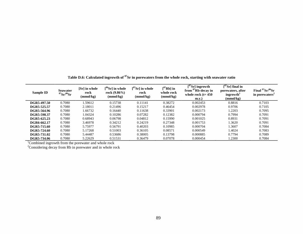
89
Table D.6: Calculated ingrowth of 87
Sr in porewaters from the whole rock, starting with seawater ratio
Sample ID Seawater 87Sr/86Sr
[Sr] in whole
rock
(mmol/kg)
[86Sr] in whole
rock (9.86%)
(mmol/kg)
[87Sr] in whole
rock
(mmol/kg)
[87Rb] in
whole rock
(mmol/kg)
[87Sr] ingrowth
from 87Rb-decay in
whole rock (t= 450
m.y.)
[87Sr] final in
porewaters, after
ingrowth1
(mmol/kg)
Final 97Sr/86Sr
in porewaters2
DGR5-497.50 0.7080 1.59612 0.15738 0.11141 0.38272 0.002453 0.8816 0.7103
DGR5-525.57 0.7080 2.18011 0.21496 0.15217 0.46454 0.002978 0.9706 0.7105
DGR5-564.96 0.7080 1.66732 0.16440 0.11638 0.33901 0.002173 1.2203 0.7095
DGR5-598.37 0.7080 1.04324 0.10286 0.07282 0.12382 0.000794 0.7994 0.7091
DGR5-625.23 0.7080 0.68943 0.06798 0.04812 0.15990 0.001025 0.8931 0.7091
DGR6-662.17 0.7080 3.46978 0.34212 0.24219 0.27348 0.001753 1.3620 0.7091
DGR5-715.60 0.7080 5.75977 0.56791 0.40203 0.10985 0.000704 1.3607 0.7084
DGR5-724.60 0.7080 5.17268 0.51003 0.36105 0.08571 0.000549 1.4024 0.7083
DGR5-731.02 0.7080 5.44487 0.53686 0.38005 0.13798 0.000885 0.7794 0.7089
DGR5-734.06 0.7080 5.22629 0.51531 0.36479 0.07078 0.000454 1.2300 0.7084 1Combined ingrowth from the porewater and whole rock
2Considering decay from Rb in porewater and in whole rock