AFRL-VA-WP-TP-2006-341 REACTIVE FLOW CONTROL OF DELTA WING VORTEX (POSTPRINT) Yong Liu, Ming Mu, J. Jim Zhu, Douglas A. Lawrence, Ephraim J. Gutmark, James H. Myatt, and Cameron A. May AUGUST 2006

Approved for public release; distribution is unlimited.

STINFO COPY

© 2006 by the Authors (except James H. Myatt) The U.S. Government is joint author of the work and has the right to use, modify, reproduce, release, perform, display, or disclose the work. AIR VEHICLES DIRECTORATE AIR FORCE MATERIEL COMMAND AIR FORCE RESEARCH LABORATORY WRIGHT-PATTERSON AIR FORCE BASE, OH 45433-7542

NOTICE AND SIGNATURE PAGE

Using Government drawings, specifications, or other data included in this document for any purpose other than Government procurement does not in any way obligate the U.S. Government. The fact that the Government formulated or supplied the drawings, specifications, or other data does not license the holder or any other person or corporation; or convey any rights or permission to manufacture, use, or sell any patented invention that may relate to them. This report was cleared for public release by the Air Force Research Laboratory Wright Site (AFRL/WS) Public Affairs Office and is available to the general public, including foreign nationals. Copies may be obtained from the Defense Technical Information Center (DTIC) (http://www.dtic.mil). AFRL-VA-WP-TP-2006-341 HAS BEEN REVIEWED AND IS APPROVED FOR PUBLICATION IN ACCORDANCE WITH ASSIGNED DISTRIBUTION STATEMENT. *//Signature// //Signature// JAMES H. MYATT, Ph.D. DEBORAH S. GRISMER, Ph.D. Senior Aerospace Engineer Chief Control Design and Analysis Branch Control Design and Analysis Branch Air Vehicles Directorate Air Vehicles Directorate //Signature// JEFFREY C. TROMP, Ph.D. Senior Technical Advisor Control Sciences Division Air Vehicles Directorate This report is published in the interest of scientific and technical information exchange, and its publication does not constitute the Government’s approval or disapproval of its ideas or findings. *Disseminated copies will show “//Signature//” stamped or typed above the signature blocks.

i

REPORT DOCUMENTATION PAGE Form Approved OMB No. 0704-0188

The public reporting burden for this collection of information is estimated to average 1 hour per response, including the time for reviewing instructions, searching existing data sources, searching existing data sources, gathering and maintaining the data needed, and completing and reviewing the collection of information. Send comments regarding this burden estimate or any other aspect of this collection of information, including suggestions for reducing this burden, to Department of Defense, Washington Headquarters Services, Directorate for Information Operations and Reports (0704-0188), 1215 Jefferson Davis Highway, Suite 1204, Arlington, VA 22202-4302. Respondents should be aware that notwithstanding any other provision of law, no person shall be subject to any penalty for failing to comply with a collection of information if it does not display a currently valid OMB control number. PLEASE DO NOT RETURN YOUR FORM TO THE ABOVE ADDRESS.

1. REPORT DATE (DD-MM-YY) 2. REPORT TYPE 3. DATES COVERED (From - To)

August 2006 Conference Paper Postprint 06/05/2001 – 03/31/2006 5a. CONTRACT NUMBER

In-house 5b. GRANT NUMBER

4. TITLE AND SUBTITLE

REACTIVE FLOW CONTROL OF DELTA WING VORTEX (POSTPRINT)

5c. PROGRAM ELEMENT NUMBER 0601102

5d. PROJECT NUMBER

A03D 5e. TASK NUMBER

6. AUTHOR(S)

Yong Liu, Ming Mu, J. Jim Zhu, and Douglas A. Lawrence (Ohio University) Ephraim J. Gutmark and Cameron A. May (University of Cincinnati) James H. Myatt (AFRL/VACA)

5f. WORK UNIT NUMBER

0B 7. PERFORMING ORGANIZATION NAME(S) AND ADDRESS(ES) 8. PERFORMING ORGANIZATION Ohio University 329 Stocker Center Athens, OH 45701 ----------------------------------------------------- University of Cincinnati Aerospace Engineering & Engineering Mechanics 799 Rhodes Hall P. O. Box 210070 Cincinnati, OH 45221-0070

Control Design and Analysis Branch (AFRL/VACA) Control Sciences Division Air Vehicles Directorate Air Force Materiel Command Air Force Research Laboratory Wright-Patterson Air Force Base, OH 45433-7542

REPORT NUMBER

AFRL-VA-WP-TP-2006-341

9. SPONSORING/MONITORING AGENCY NAME(S) AND ADDRESS(ES) 10. SPONSORING/MONITORING AGENCY ACRONYM(S)

AFRL-VA-WP Air Vehicles Directorate Air Force Research Laboratory Air Force Materiel Command Wright-Patterson Air Force Base, OH 45433-7542

11. SPONSORING/MONITORING AGENCY REPORT NUMBER(S)

AFRL-VA-WP-TP-2006-341 12. DISTRIBUTION/AVAILABILITY STATEMENT

Approved for public release; distribution is unlimited. 13. SUPPLEMENTARY NOTES

© 2006 by the Authors (except James H. Myatt). The U.S. Government is joint author of the work and has the right to use, modify, reproduce, release, perform, display, or disclose the work. Conference paper published in the Proceedings of the 2006 AIAA Guidance, Navigation, and Control Conference and Exhibit, published by AIAA. PAO Case Number: AFRL/WS 06-1786 (cleared July 19, 2006). Paper contains color.

14. ABSTRACT

In this paper, the reactive flow control of delta wing leading edge vortices using along-core pulse width modulation (PWM) flow injection is presented. Leading edge vortices on the upper surface of a delta wing can augment lift. Manipulating breakdown points of leading edge vortices can effectively change the delta wing’s lift and drag and generate attitude control torque. In this paper, a dynamic model of active flow control of vortex break down points is identified from wind tunnel data using a model scheduling method. Based on the identified model, a closed-loop active flow controller is developed. Simulation and real-time wind tunnel test show that the closed-loop controller can effectively manipulate the upper surface pressure of the delta wing, which indicates the closed-loop controller can effectively control vortex breakdown points.

15. SUBJECT TERMS flow control, delta wing, vortex

16. SECURITY CLASSIFICATION OF: 19a. NAME OF RESPONSIBLE PERSON (Monitor) a. REPORT Unclassified

b. ABSTRACT Unclassified

c. THIS PAGE Unclassified

17. LIMITATION OF ABSTRACT:

SAR

18. NUMBER OF PAGES

30 James H. Myatt 19b. TELEPHONE NUMBER (Include Area Code)

N/A Standard Form 298 (Rev. 8-98)

Prescribed by ANSI Std. Z39-18

Reactive Flow Control of Delta Wing Vortex

Yong Liu*, Ming Wu†, J. Jim Zhu‡, Douglas A. Lawrence§ School of Electrical Engineering and Computer Science, Ohio University, Athens, OH, 45701

Ephraim J. Gutmark**, Aerospace Engineering & Engineering Mechanics, University of Cincinnati, Cincinnati, OH, 45221

James H. Myatt †† Air Vehicles Directorate, Air Force Research Laboratory, Wright-Patterson AFB, OH, 45433

And

Cameron A. May‡‡ Aerospace Engineering & Engineering Mechanics, University of Cincinnati, Cincinnati, OH, 45221

In this paper, the reactive flow control of delta wing leading edge vortices using along-core pulse width modulation (PWM) flow injection is presented. Leading edge vortices on the upper surface of a delta wing can augment lift. Manipulating breakdown points of leading edge vortices can effectively change the delta wing’s lift and drag and generate attitude control torque. In this paper, a dynamic model of active flow control of vortex break down points is identified from wind tunnel data using a model scheduling method. Based on the identified model, a closed-loop active flow controller is developed. Simulation and real-time wind tunnel test show that the closed-loop controller can effectively manipulate the upper surface pressure of the delta wing, which indicates the closed-loop controller can effectively control vortex breakdown points.

Nomenclature JetA = Jet orifice area. (inch2)

µC = Jet momentum coefficient

PC = Pressure Coefficient

xe = Error state

ye = Output error

ue = Feedback control input

pK = Proportional feedback gain

iK = Integral feedback gain

oK = Observer feedback gain P = Dynamic pressure ∞P = Free stream pressure

S = Delta wing area (inch2)

* Graduate Student, School of Electrical Engineering and Computer Science, Ohio University † Graduate Student, School of Electrical Engineering and Computer Science, Ohio University. ‡ Professor, School of Electrical Engineering and Computer Science, Ohio University, corres. § Associate Professor, School of Electrical Engineering and Computer Science, Ohio University. ** Professor, Aerospace Engineering and Engineering Mechanics ††Senior Aerospace Engineer, Senior Member AIAA. ‡‡ Graduate Student, Aerospace Engineering and Engineering Mechanics

AIAA Guidance, Navigation, and Control Conference and Exhibit21 - 24 August 2006, Keystone, Colorado

AIAA 2006-6189

Copyright © 2006 by the authors. Published by the American Institute of Aeronautics and Astronautics, Inc., with permission.

1

∞U = Free stream wind velocity (inch/s)

JetV = Flow speed at jet orifice (inch/s) u = Duty cycle input u = Nominal control input δu = Broadband component of duty cycle input

u = Static duty cycle y = Dynamic pressure sensor output (V)

comy = Dynamic pressure command (V)

y = Steady dynamic pressure sensor output (V)

δy = Deviation component of dynamic pressure sensor output (V) α = Scheduling variable ρ = Air density η = Augmented error states η̂ = Observer state η~ = Observer state error ζ = Augmented output error

ζ̂ = Observer output

ζ~ = Observer output error

I. Background and Introduction he delta wing has been in the second half of the 20th century a common platform for modern high-speed civil and military aircraft due to low drag in supersonic flight as a result of the swept leading edge of the wing and high lift in subsonic flight at moderate angles of attack due to the formation of vortices over the upper surface.

At moderate to high angles of attack, there exist large leading-edge vortices propagating on the top surface of the delta wing. These vortices can effectively augment the total lift. However, during higher angle of attack flight, a phenomenon known as vortex breakdown may occur, which plays a role in limiting the performance of the aircraft. Onset of vortex breakdown is observed as the vortex diameter increases, the axial velocity of the vortex core decreases and the circumferential velocity decreases. Aft of the vortex break down location, flow becomes turbulent, which results in a rapid loss of lift. Thus, controlling vortex breakdown locations on delta wings is desirable for extending the performance envelope of delta wing aircraft.

A substantial amount of research has been dedicated to the control of aerodynamic flows using both passive and active control mechanisms. Passive vortex control devices such as vortex generators and winglets attach to the wing and require no energy input. Passive vortex control devices are designed to perform optimally over a small range of flight conditions. Active vortex control systems require energy input and can operate effectively and efficiently over a wider range of flight conditions. Types of active vortex control include fluidic control and surface control. Examples of fluidic control are leading edge injection and suction [9], trailing edge injection [14] and along-core injection [5]. Examples of surface control are movable surfaces, such as variable sweep delta wings, and micro-electromechanical devices mounted on the surface of the wing. The surface control can change the geometry of the wing for different flow conditions. Other active flow control methods, such as synthetic jet control on delta wing leading edges is also effective for changing the aerodynamic characteristics of delta wings [2] [3].

Gutmark and Guillot [5] proposed controlling the breakdown of delta wing leading edge vortices by injection into or near the vortex core. Experiments were conducted on a 60 degree half-delta wing in a wind tunnel with a Reynolds number of 260,000 based on the free stream conditions and the wing’s root chord. It was discovered that too much injection would penetrate the outer wall of the vortex core whereas too little injection would not provide enough momentum to the vortex to maintain its coherence. Along-core injection was shown to be an effective technique for manipulating vortex breakdown location.

Wind tunnel experiments were used to study reactive flow control of vortex breakdown location with along-core injection. Static pressure taps on the upper surface were used to determine vortex breakdown location. It was observed that pulse-width-modulation (PWM) flow injection with fixed flow pressure and continuous injection with

T

2

varying injection momentum are equally effective for controlling vortex breakdown. For the PWM injection, the optimized configuration of nozzle azimuth and pitch angles, injection momentum, PWM frequency and duty cycles to delay the vortex breakdown were analyzed using wind tunnel data [10]. The optimal jet configuration was the azimuth angle at 170 degrees, pitch angle at 35 degrees, momentum coefficient at 0.023, normalized modulation frequency at 1.08 based on the free stream velocity and wing’s root chord,, duty cycle at 50%, momentum coefficient at 0.023, where the nondimensional momentum coefficient is defined as

2

⎟⎟⎠

⎞⎜⎜⎝

⎛=

∞UV

SA

C jetjetu .

In this paper, closed-loop reactive control of vortex breakdown location is presented. The jet operated at the optimized configuration except the closed-loop control adjusts injection duty cycle to control the vortex breakdown location. In Section II, the experiment equipment and the data acquisition and real-time control system are introduced. In Section III, the nonlinear dynamic modeling development for delta wing active vortex control is presented. In Section IV, a trajectory linearization type gain scheduling controller based on the identified nonlinear model is developed. Simulation and real-time test results of reactive vortex control are presented in Section V.

II. Wind Tunnel Experiment, Data Acquisition and Real-time Control System Wind tunnel experiments for delta wing vortex control were conducted in the low speed wind tunnel in the

University of Cincinnati Aerospace Engineering Department’s Fluid Mechanics & Propulsion Laboratory. The wind tunnel is a subsonic closed-circuit wind tunnel manufactured by Engineering Laboratory Design Inc. located in Lake City, Minnesota. The test section has a cross-section of 2ft × 2ft and is 8ft in length. The wind tunnel is rated by the manufacturer to speeds of up to 300 ft/sec and also is equipped with a heat exchanger and a West model 3800 temperature controller so that the internal temperature can be maintained at a desired setting.

The delta wing model used in the experiment was an aluminum 60 degree sweep delta wing with a 30 leading edge bevel on the lower surface. The dimensions of the test delta wing are shown in Table 1. A top plate for the wing was designed with 96 static pressure taps on the surface in 4 span-wise rows located at 35%, 55%, 75%, and 95% of the root chord, as shown in Figure 1. A second top plate was fabricated to accommodate dynamic pressure transducers. The dynamic pressure instrument was a piezoelectric transducer manufactured by Endevco Inc. with a pressure range of 0 to 2 psia. The flow injection valve is an orifice poppet valve from Parker Valves Inc., driven by a 24 VDC signal from an Iota-1 controller also manufactured by Parker Valves Inc. Figure 2 shows the delta wing model mounted in the wind tunnel.

In the data acquisition and real-time control experiments, two different instrumentation systems were used. The first hardware used was a Labview system from National Instruments. It was used in static and dynamic pressure data acquisition. The Labview system was capable of generating PWM signals to drive the control jets and to measure the pressure sensor signals. The highest sampling rate of the Labview system used in the experiments was 4 kHz. However, the Labview system did not support real-time tasks, so it could not be used for real-time closed-loop control. The second hardware used was a Wincon/RTX system from Quanser. WinCon/RTX was a rapid-prototyping system for control system applications. RTX provided a real-time extension of the Windows OS. The Wincon toolbox, used with Simulink and Real-Time Workshop from The MathWorks, could generate real-time executable code directly from the Simulink model. In this project, Wincon 3.2, RTX 5.1 and a multi-Q PCI board were used in dynamic tests for system identification and real-time control tests. The highest sampling rate that can be achieved using the WinCon system was 2 kHz.

Table 1 Dimensions of delta wing

Sweep Angle 60°

Leading-Edge Bevel Angle 30°

Span 0.394 m

Root Chord 0.343 m

Angle of Attack 15°

Freestream Velocity 20 m/s

3

Figure 1 Delta wing control jets and static pressure sensor.

Figure 2 Wind tunnel test section for delta wing flow control.

A PWM duty cycle resolution problem was identified in the experiments. In the dynamic tests, the duty cycle was assumed to be any real number between 0% and 100%. However, using either Labview or Wincon, this assumption was not satisfied. In the Labview configuration, the highest sampling rate was 4 kHz and the desired PWM frequency is 55 Hz. Therefore, less than 80 (4000/55=72.72) different pulse widths could be generated. In the WinCon/RTX configuration, the pulse width resolution was even lower, since the highest sampling rate was only 2 kHz. The low duty cycle resolution violated the assumption for system identification. To increase the resolution of the duty cycle, a Microchip PIC18F458 microcontroller was used to generate the PWM signal at 55Hz with 10-bit (1024) resolution. Microchip 18F458 was a high end 8 bit microcontroller with highest clock rate 40 MHZ. When using the PIC18F458 as a high resolution PWM generator, the PWM signal was no longer generated by Labview or WinCon directly. Instead, an analog signal ranging between 0 to 5V, which represented 0% – 100% pulse width, was sent to the PIC18F458. The PIC18F458 picked up the command via a 10-bit built-in A/D converter, and used a 4 MHz crystal to trigger the PWM signal. Thus, the PWM signal resolution was independent of the sampling rates of the Labview and WinCon systems.

III. Nonlinear model development for vortex active flow control From wind tunnel experiment using static pressure tap, it was determined that an unsteady pressure sensor

installed at 66.7% root chord (11.43 cm from trailing edge) and at 6.35 cm span from root chord was used to indicate the vortex break down location. This sensor was under the vortex core on the delta wing upper surface, and was close to the vortex breakdown location without jet injection. When the vortex breakdown was delayed, the dynamic pressure at this position would decrease. The pressure signal is represented by the pressure coefficient pC which is defined as

⎟⎠⎞

⎜⎝⎛−= ∞∞∞

2

21/)( UPPC p ρ

The vortex breakdown was indicated by the increase of pC . The unsteady pressure sensor calibration constant was 0.070391 (mv/psi). The sensor output was amplified 1000 and then sampled by data acquisition board. The dynamic pressure at 20m/s wind speed test was 0.0462psi. The calibrated unsteady pressure coefficient was calculated as

yyC p 3075.00462.0070391.01000

=××

=

where y is the amplified pressure sensor output voltage. When the vortex breakdown was delayed, the pressure sensor output voltage increases. From the view point of control system, the system input is the duty cycle of the PWM injection, and the system output is the amplified pressure sensor output.

A nonlinear dynamic model was identified from experimental data. Methods for nonlinear control system design are typically model-based. First principles modeling may be applied to simple systems yielding parametric models that require identification and tuning of a relatively small set of parameters. Complex nonlinear phenomena often do

4

not lend themselves to this type of modeling, necessitating a black-box approach commonly referred to as system identification. Techniques for linear system identification, [6] [12] are more widely available than for the nonlinear case [7], however, linear models can only predict the behavior of a nonlinear system in a vicinity of an equilibrium point, or other nominal condition.

In order to exploit the reliability of linear system identification techniques while overcoming the inherent limitation of linear models, we employ an approach for nonlinear system identification motivated by gain scheduled control system design [7], which we refer to as model scheduling. The basic idea is to identify a set of linear models about a collection of equilibria from which a nonlinear model is constructed that instantaneously schedules the linear models based on the input signals and/or other internal variables. The overall procedure consists of the following four steps:

1) Conduct static tests on the system to acquire equilibrium data characterizing constant input signal values and associated constant steady-state output values. Characterize the output values as a function of the input values.

2) For a discrete set of equilibria, perform linear system identification to obtain a set of linear state-space models that describe the system's small-signal behavior in a vicinity of each equilibrium.

3) Interpolate or curve fit the parameters in the state-space models to yield a smoothly parameterized family of linear models.

4) Construct a nonlinear model that satisfies static and dynamic linearization requirements with respect to the parameterized family of linear models.

1. Static Test

The control jet is pulse-width modulated at normalized modulation frequency at 1.08 based on the free stream velocity and wing’s root chord, with a duty cycle that is programmable between 0% and 100% in 1/1024 0.1≈ % increments. For the static tests, PWM control jet inputs were applied for constant pulse widths ranging from 0% to 100% in 10% increments. For each fixed pulse width, three 10 second trials were performed. The raw pressure sensor voltage output was analog filtered for anti-aliasing at a cut-off frequency of 100 HZ and then sampled at a 2000 Hz rate. The first 3 seconds of data that include the unwanted transient response were discarded. The final seven seconds of data therefore comprised the steady-state response of the dynamic pressure sensor to the constant duty cycle value.

0 10 20 30 40 50 60 70 80 90 100-2.2

-2

-1.8

-1.6

-1.4

-1.2

-1

-0.8

-0.6

-0.4

Duty Cycle (%)

Vol

tage

(V)

Sensor3 Static Test Comparision

High Resolution PWM Labview Setup

Figure 3 Steady-state pressure sensor voltage vs. jet duty cycle.

For each duty cycle value, the sensor voltage time histories were averaged across the three trials and then time-averaged over the final seven seconds to yield the static steady-state value of the pressure sensor voltage for the corresponding duty cycle value. These data points with linear interpolation are plotted in Figure 3 along with error bars indicating the variance associated with the time averaging. Also plotted are the static steady-state pressure

5

sensor voltages derived from an earlier experiment that utilized the original LabView data collection system. The high-resolution PWM generator and the correction of an earlier problem with the unsteady pressure sensor combined to greatly reduce the variance in the static test data.

2. Dynamic Test The steady-state pressure sensor response versus duty cycle input depicted above, henceforth, the static curve is

used to determine the equilibria about which to conduct dynamic tests as follows. The static curve is first divided into regions which are well-approximated by a linear curve. The midpoint of each region then determines the static duty cycle value to which a broadband (random noise) perturbation is added. The width of each region then determines the amplitude of the broadband component of the duty cycle input signal. Dynamic tests were conducted on each region for broadband components with amplitude equal to 25%, 50% and 75% of the region width. The dynamic test parameters are summarized in

Table 2. The composite duty cycle input signal is denoted ( ) ( )ou t u u tδ= + in which ou is the static duty cycle

component with value given by the region midpoint and δu denotes the broadband component. The resulting

pressure sensor response denoted )(ty is decomposed as ( ) ( )oy t y y tδ= + in which oy is the static response value

corresponding to ou as determined from the static curve and the deviation component is given by ( ) ( ) oy t y t yδ = − . Figure 4 contains the time histories of the pressure sensor response and control jet duty-cycle input signal for Region 1 for perturbation amplitudes scaled to 75% of the region width.

For each region, the deviation components of both input and output signals were sampled at 2000 Hz and linear system identification algorithms were applied to the discretized signals to yield a 5th-order discrete-time linear state-space model. Two methods, eigensystem realization [6] and subspace identification [12] were employed yielding similar models. The discrete-time models were converted to a continuous-time model via the bilinear transformation[13].

Table 2 Dynamic test parameters

Range Width Nominal Duty Cycle

Noise Amp 25% width

Noise Amp 50% width

Noise Amp 75% width

Region1 0 - 14.2 14.2 7.1000 3.6 7.1 10.7

Region2 14.2 – 39.6 25.4 26.90 6.3 12.7 19

Region3 39.6 – 52.6 13 45.60 3.2 6.5 9.6

Region4 52.6 – 62.8 10.2 57.70 2.5 5.1 7.5

Region5 62.8 – 76.6 13.8 69.70 3.4 6.9 10.3

Region6 76.6 – 100 23.4 87.80 5.8 11.7 17.5

6

The continuous-time state-space models for each region, indexed by the scheduling variable oii u=α , 6,,1…=i

were cast in modal form specified by coefficient matrices:

0 1 2 3 4 5 6 7 8 9 10-2

-1.5

-1

-0.5

0

Dynamic Test Nominal Duty Cycle = 7.10 Noise Level= 10.70

Sen

sor V

olta

ge (V

)

0 1 2 3 4 5 6 7 8 9 100

20

40

60

80

100

Dut

y C

ycle

(%)

Time (Seond)

Figure 4 Pressure sensor voltage response (top) and duty-cycle input (bottom) for Region 1 dynamic test with ou =7.10% and ( )tuδ amplitude =10.70%.

( )

11 21

21 11

33 43

43 33

55

( ) ( ) 0 0 0 0( ) ( ) 0 0 0 1

( ) ,0 0 ( ) ( ) 0 00 0 ( ) ( ) 0 10 0 0 0 ( ) 0

i i

i i

i ii i

i i

i

a aa a

A Ba aa a

a

α αα α

α αα αα α

α

−⎡ ⎤ ⎡ ⎤⎢ ⎥ ⎢ ⎥⎢ ⎥ ⎢ ⎥⎢ ⎥ ⎢ ⎥= =−⎢ ⎥ ⎢ ⎥⎢ ⎥ ⎢ ⎥⎢ ⎥ ⎢ ⎥⎣ ⎦⎣ ⎦

[ ]1 2 3 4 5( ) ( ) ( ) ( ) ( ) ( ) , ( ) 0i i i i i i iC c c c c c Dα α α α α α α= =

Model parameter values are listed below in Table 3. This form directly displays the model’s eigenvalues or poles as follows

1,2 11 21 3,4 33 43 5 55( ) ( ) ( ), ( ) ( ) ( ), ( ) ( )i i i i i i i ia ja a ja a= ± = ± =λ α α α λ α α α λ α α

and the ic ’s are related to the real and imaginary parts of the residues associated with these eigenvalues in a partial fraction expansion of the model’s transfer function.

3. Parameter Interpolation

This step simply involves linear interpolation of the state space-model parameters for each region to yield state-space coefficient matrices that are now functions of the scheduling variableα (representing the PWM duty cycle in the continuous 0% - 100% range):

7

11 21

21 11

33 43

43 33

55

( ) ( ) 0 0 0( ) ( ) 0 0 0

( ) 0 0 ( ) ( ) 00 0 ( ) ( ) 00 0 0 0 ( )

a aa a

A a aa a

a

−⎡ ⎤⎢ ⎥⎢ ⎥⎢ ⎥= −⎢ ⎥⎢ ⎥⎢ ⎥⎣ ⎦

α αα α

α α αα α

α

01

( ) 011

B

⎡ ⎤⎢ ⎥⎢ ⎥⎢ ⎥=⎢ ⎥⎢ ⎥⎢ ⎥⎣ ⎦

α

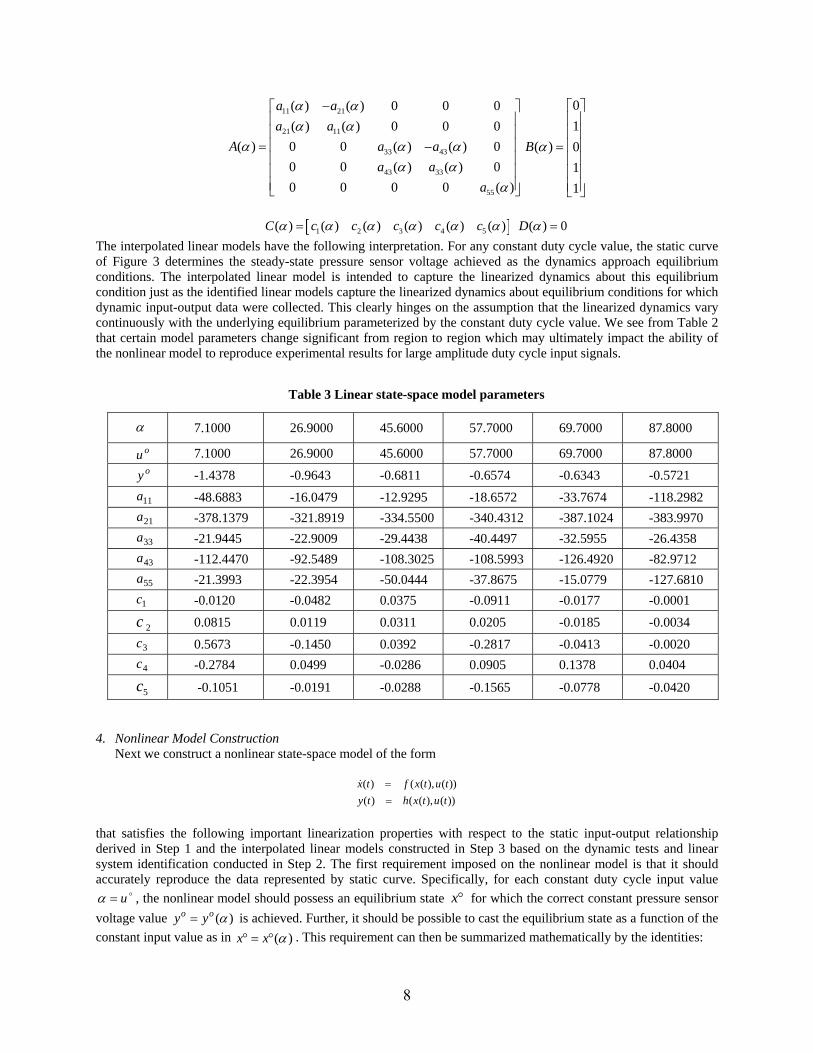
[ ]1 2 3 4 5( ) ( ) ( ) ( ) ( ) ( ) ( ) 0C c c c c c Dα α α α α α α= = The interpolated linear models have the following interpretation. For any constant duty cycle value, the static curve of Figure 3 determines the steady-state pressure sensor voltage achieved as the dynamics approach equilibrium conditions. The interpolated linear model is intended to capture the linearized dynamics about this equilibrium condition just as the identified linear models capture the linearized dynamics about equilibrium conditions for which dynamic input-output data were collected. This clearly hinges on the assumption that the linearized dynamics vary continuously with the underlying equilibrium parameterized by the constant duty cycle value. We see from Table 2 that certain model parameters change significant from region to region which may ultimately impact the ability of the nonlinear model to reproduce experimental results for large amplitude duty cycle input signals.

Table 3 Linear state-space model parameters

α 7.1000 26.9000 45.6000 57.7000 69.7000 87.8000 ou 7.1000 26.9000 45.6000 57.7000 69.7000 87.8000 oy -1.4378 -0.9643 -0.6811 -0.6574 -0.6343 -0.5721

11a -48.6883 -16.0479 -12.9295 -18.6572 -33.7674 -118.2982

21a -378.1379 -321.8919 -334.5500 -340.4312 -387.1024 -383.9970

33a -21.9445 -22.9009 -29.4438 -40.4497 -32.5955 -26.4358

43a -112.4470 -92.5489 -108.3025 -108.5993 -126.4920 -82.9712

55a -21.3993 -22.3954 -50.0444 -37.8675 -15.0779 -127.6810

1c -0.0120 -0.0482 0.0375 -0.0911 -0.0177 -0.0001

2c 0.0815 0.0119 0.0311 0.0205 -0.0185 -0.0034

3c 0.5673 -0.1450 0.0392 -0.2817 -0.0413 -0.0020

4c -0.2784 0.0499 -0.0286 0.0905 0.1378 0.0404

5c -0.1051 -0.0191 -0.0288 -0.1565 -0.0778 -0.0420

4. Nonlinear Model Construction

Next we construct a nonlinear state-space model of the form

( ) ( ( ), ( ))( ) ( ( ), ( ))

x t f x t u ty t h x t u t

==

that satisfies the following important linearization properties with respect to the static input-output relationship derived in Step 1 and the interpolated linear models constructed in Step 3 based on the dynamic tests and linear system identification conducted in Step 2. The first requirement imposed on the nonlinear model is that it should accurately reproduce the data represented by static curve. Specifically, for each constant duty cycle input value

u=α , the nonlinear model should possess an equilibrium state x° for which the correct constant pressure sensor voltage value )(αoo yy = is achieved. Further, it should be possible to cast the equilibrium state as a function of the constant input value as in ( )x x° = ° α . This requirement can then be summarized mathematically by the identities:

8

( ( ), ) 0( ( ), ) ( ).

f xh x y

α αα α α

° =° = °

The second requirement imposed on the nonlinear model is that its linearization about any equilibrium should exactly match the (interpolated) linear model for that equilibrium. This ensures that the small-signal behavior of the nonlinear model about any equilibrium is governed by the associated linear model. Writing the nonlinear model’s linearization about an equilibrium corresponding to a constant duty cycle input value u= °α as

( ) ( ( ), ) ( ) ( ( ), ) ( )

( ) ( ( ), ) ( ) ( ( ), ) ( )

f fx t x x t x u tx uh hy t x x t x u tx u

δ δ δ

δ δ δ

α α α α

α α α α

∂ ∂= ° + °

∂ ∂∂ ∂

= ° + °∂ ∂

it is clear that the second requirement is equivalent to the following identities:

( ( ), ) ( ) ( ( ), ) ( )

( ( ), ) ( ) ( ( ), ) ( ).

f fx A x Bx uh hx C x Dx u

α α α α α α

α α α α α α

∂ ∂° = ° =

∂ ∂∂ ∂

° = ° =∂ ∂

Nontrivial existence conditions must be satisfied in order for these requirements to be met. Here we proceed directly to the specification of a nonlinear model with the requisite properties. First, we point out that since the modeling objective is to predict input-output behavior from jet duty cycle to pressure sensor voltage and since the underlying model state has no physical significance, a coordinate transformation on the model state does not interfere with the ultimate modeling goal. In the present context consider an alternate interpolated linear model specified by

1ˆ ˆˆ ˆ( ) ( ), ( ) ( ) ( ), ( ) ( ) ( ), ( ) ( )A A B A B C C A D Dα α α α α α α α α α−= = = = .

The associated transfer function of the transformed model matches that of the original interpolated linear model as can be readily verified:

[ ]( )

[ ]

1

11

11

1

ˆ ˆˆ ˆ ˆ( , ) ( ) ( ) ( ) ( )

( ) ( ) ( ) ( ) ( ) ( )

( ) ( ) ( ) ( ) ( ) ( )

( ) ( ) ( ) ( )( , ).

H s C sI A B D

C A sI A A B D

C A sI A A B D

C sI A B DH s

α α α α α

α α α α α α

α α α α α α

α α α αα

−

−−

−−

−

⎡ ⎤= − +⎣ ⎦

= − +

⎡ ⎤= − +⎣ ⎦

= − +

=

Next, consider the nonlinear model specified by the following functions:

[ ][ ]1

( , ) ( )

( , ) ( ) ( ) ( )

f x u A x Bu

h x u C A x B y

α

α α α α−

= +

= + + °

in which α is produced by any function ( , )x uϕ that satisfies ( ( ), )x° =ϕ α α α and we have explicitly incorporated the fact that ( ) BB =α , constant, and ( ) 0=αD . The first requirement is satisfied for the equilibrium state

0

( ) 0x Bα

α ααα

⎡ ⎤⎢ ⎥−⎢ ⎥⎢ ⎥° = − =⎢ ⎥−⎢ ⎥⎢ ⎥−⎣ ⎦

9

from which it follows that 2 4 5( , ) , , ,x u u x x xϕ = − − − are valid choices for the function ( , )⋅ ⋅ϕ . As for the second requirement, using ( ) 0x B° + =α α we see that

[ ]( ( ), ) ( ( ( ), )) ( ( ), ) ( ) ( ( ( ), ))

( )ˆ( )

f Ax x x x B A xx x

A

A

ϕα α ϕ α α α α α α ϕ α ααα

α

∂ ∂ ∂° = ° ° ° + + °

∂ ∂ ∂=

=

[ ]( ( ), ) ( ( ( ), )) ( ( ), ) ( ) ( ( ( ), ))

( )ˆ ( )

f Ax x x x B A x Bu u

A B

B

ϕα α ϕ α α α α α α ϕ α ααα

α

∂ ∂ ∂° = ° ° ° + + °

∂ ∂ ∂=

=

For the output equation, provided that the following necessary condition is satisfied by the static curve and interpolated linear models

1

1

( ) ( ) ( ) ( ) ( )

( ) ( )

y C A B D

C A B

α α α α αα

α α

−

−

∂ °= − +

∂= −

we have

[ ]1

1

1 1

( )( ( ), ) ( ( ( ), )) ( ( ), ) ( )

( ) ( ) ( ( ), ) ( ) ( ( ), )

( ) ( ) ( ) ( ) ( ) ( ( ), )

ˆ ( )

h CAx x x x Bx x

yC A I B x xx x

yC A C A B xx

C

ϕα α ϕ α α α α α αα

ϕ ϕα α α α α α ααϕα α α α α α α

α

α

−

−

− −

∂ ∂ ∂° = ° ° ° +

∂ ∂ ∂∂ ∂ ° ∂⎡ ⎤+ + ° + °⎢ ⎥∂ ∂ ∂⎣ ⎦

∂ ° ∂⎡ ⎤= + + °⎢ ⎥∂ ∂⎣ ⎦

=

and

[ ]1

1

( )( ( ), ) ( ( ( ), )) ( ( ), ) ( )

( ) ( ) ( ) ( ( ), )

0( )

ˆ ( )

h CAx x x x Bu u

yC A B xu

D

D

ϕα α ϕ α α α α α αα

ϕα α α α αα

α

α

−

−

∂ ∂ ∂° = ° ° ° +

∂ ∂ ∂∂ ° ∂⎡ ⎤+ + °⎢ ⎥∂ ∂⎣ ⎦

==

=

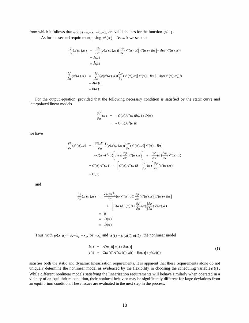
Thus, with 2 4( , ) , , ,x u u x x= − −ϕ or 5x− and ( ) ( ( ), ( ))t x t u t=α ϕ , the nonlinear model

[ ][ ]1

( ) ( ( )) ( ) ( )

( ) ( ( )) ( ( )) ( ) ( ) ( ( ))

x t A t x t Bu t

y t C t A t x t B t y t

α

α α α α−

= +

= + + ° (1)

satisfies both the static and dynamic linearization requirements. It is apparent that these requirements alone do not uniquely determine the nonlinear model as evidenced by the flexibility in choosing the scheduling variable ( )tα . While different nonlinear models satisfying the linearization requirements will behave similarly when operated in a vicinity of an equilibrium condition, their nonlocal behavior may be significantly different for large deviations from an equilibrium condition. These issues are evaluated in the next step in the process.

10

IV. Delta Wing Vortex Breakdown Location Controller Design The closed-loop controller has a trajectory linearization like structure. Trajectory linearization control (TLC) is a

nonlinear control method based on linearization along a nominal trajectory. The structure of TLC is illustrated in Figure 5. A TLC controller consists of two components: a pseudo inversion of the plant that generates the nominal control input (open-loop control), and a linear time-varying feedback regulator that stabilizes and decouples the tracking error dynamics (closed-loop control). The nonlinear tracking and decoupling control by trajectory linearization can be viewed as the ideal gain-scheduling controller designed at every point on the trajectory. Therefore the TLC provides robust stability and performance along the trajectory. TLC has been successfully applied in flight control [4, 11, 15, 16, 17] and mobile robot control [8].

The reactive flow control system of delta-wing vortices was a TLC type system. In the controller design, it was assumed that the gain scheduling variable (such as the pressure command) changed slowly compared with the system dynamics. Based on this assumption, the pseudo-inverse of the plant model was achieved by interpolating the static test results. By looking up the static test results, a nominal duty cycle command was generated, which would put the pressure in the vicinity of the commanded pressure at the sensor location. Based on the slowly varying scheduling variable assumption, at each operation region, the error dynamics were approximated by the local linear models identified from Section 3.2. For each operating region, a linear feedback controller is designed to stabilize the operating error about the operating point, i.e. drive the error to zero asymptotically. Then a nonlinear feedback stabilizer is designed by interpolating gains of these linear feedback controllers with the scheduling variable. Since the error state cannot be measured directly, a gain-scheduling nonlinear error state observer was designed to observe the error state from the output error in a manner similar to the nonlinear feedback stabilizer design. The structure of the reactive flow control system for the delta-wing vortex is illustrated in Figure 6.

µµ~

Pseudo-InversePlant Model

Stabilizing Controller

Nonlinear Plant Modelcomy

µ

y

Figure 5 Trajectory linearization control structure.

pK

Plant

Plant ModelPseudo Inverse

- ∫u y

comy u

iK

Error State Observer

pK pK

Plant

Plant ModelPseudo Inverse

- ∫u y

comy u

iK iK

Error State Observer

Figure 6 Reactive flow control system for the delta-wing vortex.

11

1. Closed-loop Controller Design The gain-scheduled nonlinear model (1) can be rewritten as

( ) ( )( )

( ) ( ) ( ) ( ) ( ) ( )

1

1

ˆ ˆˆˆ ˆ ( ) ( ) ( )

whereˆ ˆˆ, ( ) ,

x A B u

y C x C A B y

A A B A B C C A

α α

α α α α α

α α α α α α α

−

−

= +

= + +

= = =

(2)

For a given command comy , by looking up the static test curve, the scheduling variable and equilibrium point of the system are determined, such that

αBxo −= when α=ou (3a)

At the equilibrium point,

( )αocom yy = (3b)

Assuming the scheduling variable is a constant, the system dynamics can be linearized at the equilibrium point. Define the error state, output error and feedback control input as

( ) ( ) ( )ααα ou

oy

ox uueyyexxe −=−=−= ,,

The error dynamics at the nominal state can be written as

( ) ( )( )

ˆ ˆ

ˆx x u

y x

e A e B e

e C e

α α

α

= ⋅ +

= (4)

To introduce integral output feedback to the error dynamics, we augment the error states and output as

, x y

y y

e e

e eη ζ

⎡ ⎤ ⎡ ⎤= =⎢ ⎥ ⎢ ⎥⎢ ⎥ ⎢ ⎥⎣ ⎦ ⎣ ⎦∫ ∫

Then the augmented error dynamics is

( )( )

( )

( )

ˆ ˆˆ 0

ˆ 01

u

A B eC 0

C

α αη ηα

αζ η

⎡ ⎤ ⎡ ⎤= +⎢ ⎥ ⎢ ⎥⎢ ⎥ ⎣ ⎦⎣ ⎦⎡ ⎤

= ⎢ ⎥⎣ ⎦

0

0

(5)

Design the feedback control law as

u p ie K K η⎡ ⎤= ⎣ ⎦

Then the closed-loop system dynamics are

( ) ( ) ( )( )

ˆ ˆ ˆ

ˆ 0P iA B K B K

C

α α αη η

α

⎡ ⎤+= ⎢ ⎥⎢ ⎥⎣ ⎦

(6)

12

If the matrix ( ) ( )( ) ⎥

⎦

⎤⎢⎣

⎡

0ˆˆˆ

ααα

CBA has full rank, the augmented system is controllable. We can place the closed-loop

eigenvalues at any desired position.

2. Error State Observer Design The error state observer is designed for the augmented error dynamics (5). Suppose the observer dynamics are

( )( )

( )

( ) ηαζ

αηααη

ˆ10ˆˆ

0

ˆˆ

ˆˆ

ˆ

⎥⎥⎦

⎤

⎢⎢⎣

⎡=

⎥⎥⎦

⎤

⎢⎢⎣

⎡+

⎥⎥⎦

⎤

⎢⎢⎣

⎡=

0

0

C

eB0C

Au

(7)

where ˆ η is the observer state variables, ˆ ζ is the observer output.

Define ηηη ˆ~ −= and ξξξ ˆ~−= , then the error dynamics of the observer is

( )( )( )

ˆ 0ˆ

ˆ 01

A

C 0

C

αη η

α

αζ η

⎡ ⎤⎢ ⎥=⎢ ⎥⎣ ⎦⎡ ⎤

= ⎢ ⎥⎢ ⎥⎣ ⎦0

(8)

By introducing a feedback law to stabilize the observer error dynamics, the error dynamics of the observer become

( )( )( )

ˆ 0ˆ

ˆ 00 1

o

AK

C 0

C

αη η ζ

α

αζ η

⎡ ⎤⎢ ⎥= +⎢ ⎥⎣ ⎦⎡ ⎤

= ⎢ ⎥⎢ ⎥⎣ ⎦

(9)

The system (5) is observable, so the augmented system is also observable. We can design the observer feedback gain to put the eigenvalues of the closed-loop observer dynamics in the desired locations.

The total control input (duty cycle) is ( ) ˆ p iu u K Kα η⎡ ⎤= + ⎣ ⎦

V. Delta Wing Vortex Breakdown Location Control Simulation and Real-time Wind Tunnel Test

The closed-loop vortex breakdown controller was simulated in Simulink first, and then tested in real-time wind tunnel experiments. The feedback gains are listed in

Table 4. In the controller implementation, the gain scheduling variable is chosen as the nominal control input.

The nominal control input was filtered by a low pass filter, and then fed into the gain scheduling controller and gain scheduling model. The observer gains are listed in Table 5.

1. Simulation Result

Figure 7 shows the simulation diagram with augmented error state observer. Figure 8, Figure 9 and Figure 10

show simulation results with the augmented observer.

13

Table 4 Gain scheduling feedback gains

α 7.1000 26.9000 45.6000 57.7000 69.7000 87.8000

0.5762 0.7618 0.6471 0.5845 0.5822 0.0728

0.8711 0.7954 0.9191 0.9430 0.9285 0.9518

-0.1775 -0.0193 -0.1020 -0.0757 -0.0983 -0.0284

0.1831 0.0678 0.0450 -0.0021 0.0176 0.0059

pK

-0.7396 -0.0262 -0.0593 -0.0179 -0.0793 -0.0001

)10( 2×iK -32.9125 -14.0684 -51.9755 -1.8490 -3.4307 -21.0059

Table 5 Augmented error state observer gains

α 7.1000 26.9000 45.6000 57.7000 69.7000 87.8000

0.1122 0.1794 -0.0268 0.1228 0.1129 1.5110

-0.1398 0.1421 -0.2568 0.0603 0.6255 3.9057

-0.0002 0.0011 -0.0005 0.0001 -0.0009 -0.0006

0.0002 -0.0002 0.0038 -0.0005 -0.0011 -0.0011

0 0.0005 0.0002 0 0 -0.0003

1oK

)10( 2×

0 0 0 0 0 0

0 0 0 0 0 0

0 0 0 0 0 0

0 0 0 0 0 0

0 0 0 0 0 0

0 0 0 0 0 0

2oK

0.0050 0.0050 0.0050 0.0050 0.0050 0.0050

*The observer gain is ⎥⎦

⎤⎢⎣

⎡=

2

1

o

oo K

KK

14

yerror1

y

xerror

u

integralerror

error_state

orstate_estima

To_workspace

controinput

To Workspace4

rorstate_estima

To Workspace3

uinput

To Workspace2

command

To Workspace1

youtput

To Workspace

Terminator

x

initial x

x_f iltering

Subsystem2

x

initial x

x_f iltering

Subsystem1

Scheduling Variable Feedback Gain

Subsystem

Step

Scope

Saturation

Reshape1

Reshape

Product1

MatrixMultiply

Product

u

scheduling v ariable

Initial Condition

x-state

y

Ahead

Bhead

Chead

Plant Model

Scheduling Variable

Initial Condition

y error

A

B

C

ex_estimate

Observer

-1.0

Model Initial Condition2

-C-

Model Initial Condition

Look-UpTable of Nominal Control2

Look-UpTable of Nominal Control1

Look-UpTable of Nominal Control

1s

Integrator

-C-

Initial Condition1

1

Gain

12.86

Display2

em

-[0 1 0 1 1]

B Matrix[5x1]

[5x1][5x1]

5

5

6 [1x6]

[1x6]

6 6

5 [5x1]

[5x1]

[5x1]

[5x1] [5x1][5x1][5x1]

2

2

2

[6x1]

[6x1]

[6x1]

[6x1] [5x1]

[5x1] [6x1]

[6x1]

Figure 7 Closed-loop control simulation with augmented error state observer.

Figure 8 Closed-loop control simulation with augmented error state observer: command and output.

0 0.5 1 1.5 2 2.5 3 3.5 4 4.5 5-1.35

-1.3

-1.25

-1.2

-1.15

-1.1

-1.05

-1

-0.95

-0.9

Time (Second)

Ses

or V

olta

ge (V

)

Command and Output

ResponseCommand

15

2. Real-time Wind Tunnel Experiment

In the real-time wind tunnel experiment, the hardware is the Wincon/RTX system with a high resolution PWM generator. The Simulink diagram is shown in Figure 11. In the real-time test, the sensor output voltage was filtered by the second order low pass filter. The damping ratio is 0.707, and the bandwidth is 13 rad/s. The filtered sensor output was used as the measurement to feed into the closed-loop controller. The scheduling variable was chosen as

0 0.5 1 1.5 2 2.5 3 3.5 4 4.5 5-0.06

-0.04

-0.02

0

0.02

0.04

0.06

Time (Second)

Erro

r Sta

te E

stim

atio

n

Error State Estimation

Figure 9 Closed-loop control simulation with augmented error state observer: error state estimation.

0 0.5 1 1.5 2 2.5 3 3.5 4 4.5 50

10

20

30

40

50

60

Time (Second)

Dut

yCyc

le (p

erce

nt)

Control Input

Figure 10 Closed-loop control simulation with augmented error state observer: control input.

16

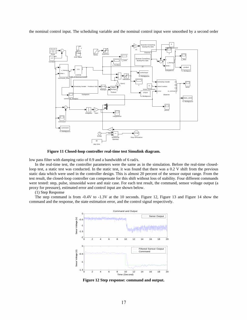
the nominal control input. The scheduling variable and the nominal control input were smoothed by a second order

low pass filter with damping ratio of 0.9 and a bandwidth of 6 rad/s. In the real-time test, the controller parameters were the same as in the simulation. Before the real-time closed-

loop test, a static test was conducted. In the static test, it was found that there was a 0.2 V shift from the previous static data which were used in the controller design. This is almost 20 percent of the sensor output range. From the test result, the closed-loop controller can compensate for this shift without loss of stability. Four different commands were tested: step, pulse, sinusoidal wave and stair case. For each test result, the command, sensor voltage output (a proxy for pressure), estimated error and control input are shown below.

(1) Step Response The step command is from -0.4V to -1.3V at the 10 seconds. Figure 12, Figure 13 and Figure 14 show the

command and the response, the state estimation error, and the control signal respectively.

yerror1

y_filterQuanser ConsultingMultiQ-PCI ADC

y1

y

xerror

u_norm

u_feedback

-K-

u2

u

40

stop time

integralerror

command_filterplot

x

initial x

x_f iltering

command_filter

command

controinput

To Workspace4

rorstate_estima

To Workspace3

uinput

To Workspace2

command

To Workspace1

youtput

To Workspace

x

initial x

x_f iltering

Subsystem2

Scheduling Variable Feedback Gain

Subsystem

STOP

Stop Simulation

Step

Sine Wave

Saturation

Reshape

>=

RelationalOperator

Ramp QuantizerPulseGenerator

MatrixMultiply

Product

Scheduling Variable

Initial Condition

y error

A

B

C

ex_estimate

Observer

???

Look-UpTable of Nominal Control

1s

Integrator

0

Initial Condition3

-C-

Initial Condition1

1 Gain2

1

Gain1

1

Gain

-1.2

Constant

Clock1

Quanser ConsultingMultiQ-PCI DAC

Channel 2

Figure 11 Closed-loop controller real-time test Simulink diagram.

0 2 4 6 8 10 12 14 16 18 20-2

-1.5

-1

-0.5

0Command and Output

Ses

or V

olta

ge (V

) Senor Output

0 2 4 6 8 10 12 14 16 18 20-1.5

-1

-0.5

0

Time (Second)

Ses

or V

olta

ge (V

) Filtered Sensor OutputCommand

Figure 12 Step response: command and output.

17

0 2 4 6 8 10 12 14 16 18 20-50

0

50Estimated State Error

0 2 4 6 8 10 12 14 16 18 20-20

0

20

0 2 4 6 8 10 12 14 16 18 20-5

0

5

0 2 4 6 8 10 12 14 16 18 20-2

0

2

0 2 4 6 8 10 12 14 16 18 20-2

0

2

Time (Second)

Figure 13 Step response: state estimation error.

0 2 4 6 8 10 12 14 16 18 200

10

20

30

40

50

60

70

80

90

100

Time (Second)

Dut

yCyc

le (p

erce

nt)

Control Input

Figure 14 Step response: control input.

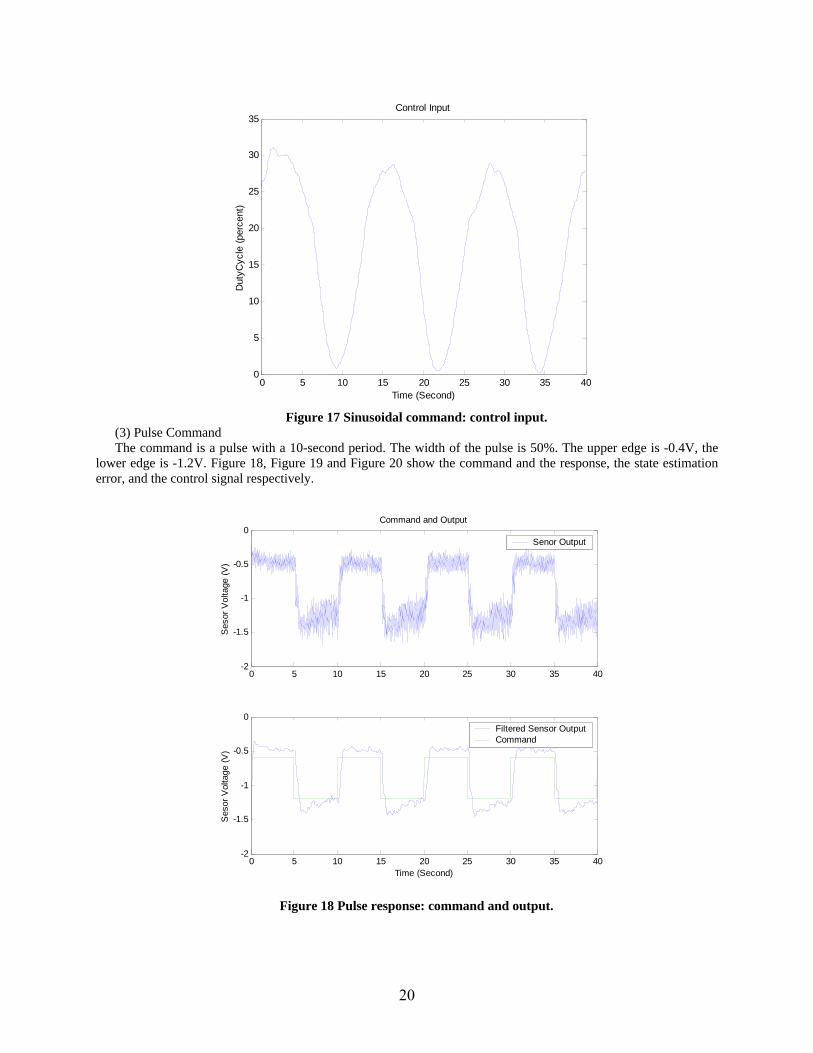
(2) Sinusoidal Wave Command The command is a sinusoidal signal with a frequency of 0.5 rad/s. The amplitude of the sinusoidal signal is 0.3V,

and the bias is -1V. Figure 15, Figure 16 and Figure 17 show the command and the response, the state estimation error and the control signal, respectively.

18

0 5 10 15 20 25 30 35 40-2

-1.5

-1

-0.5

0Command and Output

Ses

or V

olta

ge (V

)

Senor Output

0 5 10 15 20 25 30 35 40-1.5

-1

-0.5

Time (Second)

Ses

or V

olta

ge (V

)

Filtered Sensor OutputCommand

Figure 15 Sinusoidal command: command and output.

0 5 10 15 20 25 30 35 40-0.5

0

0.5Estimated State Error

0 5 10 15 20 25 30 35 40-0.5

0

0.5

0 5 10 15 20 25 30 35 40-0.2

0

0.2

0 5 10 15 20 25 30 35 40-0.5

0

0.5

0 5 10 15 20 25 30 35 40-2

0

2

Time (Second)

Figure 16 Sinusoidal command: state estimation error.

19

0 5 10 15 20 25 30 35 400

5

10

15

20

25

30

35

Time (Second)

Dut

yCyc

le (p

erce

nt)

Control Input

Figure 17 Sinusoidal command: control input.

(3) Pulse Command The command is a pulse with a 10-second period. The width of the pulse is 50%. The upper edge is -0.4V, the

lower edge is -1.2V. Figure 18, Figure 19 and Figure 20 show the command and the response, the state estimation error, and the control signal respectively.

0 5 10 15 20 25 30 35 40-2

-1.5

-1

-0.5

0Command and Output

Ses

or V

olta

ge (V

)

Senor Output

0 5 10 15 20 25 30 35 40-2

-1.5

-1

-0.5

0

Time (Second)

Ses

or V

olta

ge (V

)

Filtered Sensor OutputCommand

Figure 18 Pulse response: command and output.

20

0 5 10 15 20 25 30 35 40-10

0

10Estimated State Error

0 5 10 15 20 25 30 35 40-10

0

10

0 5 10 15 20 25 30 35 40-1

0

1

0 5 10 15 20 25 30 35 40-1

0

1

0 5 10 15 20 25 30 35 40-5

0

5

Time (Second)

Figure 19 Pulse response: state estimation error.

0 5 10 15 20 25 30 35 400

10

20

30

40

50

60

70

80

90

Time (Second)

Dut

yCyc

le (p

erce

nt)

Control Input

Figure 20 Pulse response: control input.

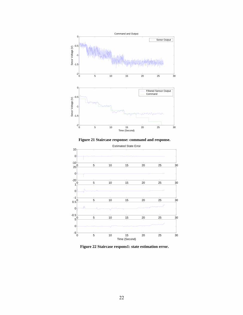
(4) Staircase Response The command is a staircase starting from -0.6V, with step size -0.2V. Figure 21, Figure 22 and Figure 23 show

the command and the response, the state estimation error, and the control signal respectively. The controller saturates after 17 seconds. The duty cycle is 0%, there is no injection to delay the vortex breakdown. The delta wing upper surface pressure reaches its limit at this point.

21

0 5 10 15 20 25 30-2

-1.5

-1

-0.5

0Command and Output

Ses

or V

olta

ge (V

)

Senor Output

0 5 10 15 20 25 30-2

-1.5

-1

-0.5

0

Time (Second)

Ses

or V

olta

ge (V

)

Filtered Sensor OutputCommand

Figure 21 Staircase response: command and response.

0 5 10 15 20 25 30-10

0

10Estimated State Error

0 5 10 15 20 25 30-20

0

20

0 5 10 15 20 25 30-1

0

1

0 5 10 15 20 25 30-0.5

0

0.5

0 5 10 15 20 25 30-5

0

5

Time (Second)

Figure 22 Staircase respons1: state estimation error.

22

0 5 10 15 20 25 300

10

20

30

40

50

60

70

80

90

Time (Second)

Dut

yCyc

le (p

erce

nt)

Control Input

Figure 23 Staircase response: control input.

VI. Conclusion and Future Work In this paper, the modeling and the reactive flow control of delta wing vortex breakdown locations have been

presented. A dynamic model of active flow control of vortex breakdown locations is identified using a model scheduling method1. Based on the identified model, a reactive flow controller is developed and real-time tested in a wind tunnel. Simulation and the real-time wind tunnel test show that the reactive controller can effectively manipulate the upper surface pressure of the delta wing in the presence of turbulence levels commonly found in subsonic wind tunnels.

The relationship between individual surface pressures and aerodynamic forces and moments necessary for flight control design was not explored. In future work, a high-bandwidth force and moment balance will be used to directly measure forces and moments generated by reactive vortex breakdown location control. A flying delta wing aircraft using reactive flow control will be developed and tested in the future.

Acknowledgment The authors gratefully acknowledge the financial support provided by the Ohio Dayton Area Graduate Studies

Institute (DAGSI).

References 1Allwine, D.A., Strahler, J.A., Lawrence, D.A., Jenkins, J.E., and Myatt, J.H., "Nonlinear Modeling of Unsteady

Aerodynamics at High Angle of Attack," AIAA Paper 2004-5275, AIAA Atmospheric Flight Mechanics Conference, Providence, RI, Aug. 2004.

2Amitay, M., Washburn, A.E., Anders, S.G., Parekh, D.E., and Glezer, A., “Active Flow Control on the Stingray UAV: Transient Behavior,” AIAA Paper 2003-4001, 33rd AIAA Fluid Dynamics Conference, Orlando, FL, June 2003.

3Amitay, M., Washburn, A.E., Anders, S.G., and Parekh, D.E., “Active Flow Control on the Stingray Uninhabited Air Vehicle: Transient Behavior,” AIAA Journal, Vol. 42. No. 11, Nov. 2004, pp. 2205-2215.

4 Bevacqua, T., Best, E., Huizenga, A., Cooper, D., and Zhu, J.J., “Improved Trajectory Linearization Flight Controller for Reusable Launch Vehicles,” AIAA Paper 2004-0875, 42nd Aerospace Sciences Meeting, Reno, NV, Jan. 2004.

5 E. Gutmark and S. Guillot, “Control of Vortex Breakdown over Highly Swept Wings”, AIAA J., Vol. 43, No. 9, pp. 2065-2069, Sept. 2005.

6 Juang, J.-N. and Pappa, R.S. “An Eigensystem Realization Algorithm for Modal Parameter Identification and Model Reduction,” AIAA Journal of Guidance and Control, and Dynamics, Vol. 8, No. 5, May 1985, pp. 620 - 627.

23

7 Lawrence, D.A. and Rugh, W.J., “Gain Scheduling Dynamic Linear Controllers for a Nonlinear Plant,” Automatica, Vol. 31, No. 3, Mar. 1995, pp. 381 – 390.

8Liu, Y., Wu, X., Zhu, J., and Lew, J., "Omni-Directional Mobile Robot Controller Design by Trajectory Linearization," Proceedings of the American Control Conference, Vol. 4, Denver, CO, June 2003, pp. 3423-3428.

9 Maines, B. H., Moeller, B., and Rediniotis, O.K., “The Effects of Leading Edge Suction on Delta Wing Vortex Breakdown", AIAA Paper 99-0128, 37th Aerospace Sciences Meeting, Reno, NV, Jan. 1999.

10 May, C. and Gutmark, E. J., “High angle of attack flight control of delta wings using vortex actuators”, Proceedings of 43rd AIAA Aerospace Sciences Meeting and Exhibit, 2005, AIAA-2005-1232.

11 Mickle, M.C. and Zhu, J.J, “Bank-to-Turn Roll-Yaw-Pitch Autopilot Design Using Dynamic Nonlinear Inversion and PD-Eigenvalue Assignment,” Proceedings of the American Control Conference, Vol. 2, Chicago, IL, June 2000, pp. 1359-1364.

12Moonen, M., De Moor, B., Vanderberghe, L., and Vandewalle, J., “On and Off-line Identification of Linear State Space Models,” International Journal of Control, Vol. 49, No. 1, 1989, pp. 219 - 232.

13 Phillips C. L. and Nagle H.T. , Digital Control System Analysis and Design, 2nd edition, Prentice-Hall, Englewood Cliffs, NJ, 1992.

14 Watry, C. and Helin, H., “Effects of Trailing Edge Jet Entrainment on Delta Wing Vortices,” AIAA Paper 94-0072, 32nd Aerospace Sciences Meeting, Reno, NV, Jan. 1994.

15Wu, X., Liu, Y., and Zhu, J.J., "Design and Real Time Testing of a Trajectory Linearization Flight Controller for the 'Quanser UFO,'" Proceedings of the American Control Conference, Vol. 5, Denver, CO, June 2003, pp. 3913-3918.

16Zhu, J.J. and Huizenga, A.B., "A Type Two Trajectory Linearization Controller for a Reusable Launch Vehicle - A Singular Perturbation Approach," AIAA Paper 2004-5184, AIAA Atmospheric Flight Mechanics Conference, Providence, RI, Aug. 2004.

17 Zhu, J. , Hodel, A.S., Funston, K., and Hall, C.E. “X-33 Entry Flight Controller Design by Trajectory Linearization - A Singular Perturbational Approach,” AAS-01-012, American Astronautical Society Guidance and Control Conference, Breckenridge, Colorado, Jan. 2001, also in Guidance and Control 2001, Advances in the Astronautical Sciences, Vol. 107, , American Astronautical Society, pp. 151-170.

24