Embed Size (px)
Citation preview

OXIRED 02
– Work Package 3 –
Reactive Transport
Modeling
Report on Task 3.4
submitted to
by
UIT GmbH DresdenZum Windkanal 21, D-01109 Dresden, Germany
Project financed by:
Dresden, Mar 2011


DELIVERABLE D 3.4
Reactive Transport Modelingof
TUB Column Tests
AUTHORS: Dr. Harald KalkaDr. Jana Nicolai
CONTACT: Dr. Harald KalkaPhone: +49-351-8 86 46 40Fax: +49-351-8 86 57 73E-Mail: [email protected]
PROJECT PARTNER: Technische Universität Berlin
Dr. Traugott ScheyttDr. Dirk RadnyBeate Müller


Reactive Transport Modeling – Mar 2011 3
CONTENTS
1 INTRODUCTION....................................................................................................................... 51.1 Background and Objectives............................................................................................ 51.2 The Model ...................................................................................................................... 61.3 List of Abbreviations...................................................................................................... 7
2 EXPERIMENTAL SETUP AND MODEL INPUT ........................................................................... 92.1 Experimental Setup ........................................................................................................ 92.2 Model Configuration and Input Parameters ................................................................. 11
2.2.1 Geometry & Hydraulics ........................................................................................ 112.2.2 Two-Layer Model ................................................................................................. 132.2.3 Aqueous Solutions ................................................................................................ 142.2.4 Thermodynamic Database..................................................................................... 15
3 HYDRAULICS AND HYDROCHEMISTRY ................................................................................ 173.1 Advection and Dispersion ............................................................................................ 173.2 Cation Exchange........................................................................................................... 183.3 Mineral Phases ............................................................................................................. 22
3.3.1 Theoretical Background ........................................................................................ 223.3.2 Model Calculations ............................................................................................... 233.3.3 Comparison of three Calcite-Precipitation Models............................................... 26
4 REDOX REACTIONS .............................................................................................................. 274.1 Theoretical Background ............................................................................................... 274.2 Experimental Evidence for Redox Reactions............................................................... 294.3 Redox Sequences in the Column Tests ........................................................................ 304.4 Biodegradation and Enzyme Kinetics .......................................................................... 31
4.4.1 Conceptual Model ................................................................................................. 314.4.2 Model Parameters and Initial Conditions.............................................................. 34
4.5 Application and Model Results .................................................................................... 374.5.1 Model Calculations versus Experiments............................................................... 374.5.2 Interpretation – Redox Zonation inside Columns ................................................. 414.5.3 Limits and Benefits ............................................................................................... 43
5 SUMMARY ............................................................................................................................ 45
REFERENCES................................................................................................................................ 47
APPENDIX .................................................................................................... 49
A REACTIVE TRANSPORT ........................................................................................................ 51A.1 Definition of the System............................................................................................... 51
A.1.1 Aqueous and Mineral Phases ................................................................................ 51A.1.2 Main Equations ..................................................................................................... 52
A.2 Transport Phenomena................................................................................................... 53A.2.1 Advection in a Homogeneous System................................................................... 53A.2.2 Advection in a Heterogeneous System.................................................................. 54A.2.3 Dispersion ............................................................................................................. 55A.2.4 Numerical Model versus Analytical Solution ....................................................... 57

Reactive Transport Modeling – Mar 20114
A.3 The Software................................................................................................................. 59
B ENZYME KINETICS ............................................................................................................... 61B.1 Michaelis-Menten Equation ......................................................................................... 61B.2 Enzyme Inhibition – HALDANE Equation ..................................................................... 63B.3 Microbial Growth Dynamics – MONOD Kinetics......................................................... 65

Reactive Transport Modeling – Mar 2011 5
1 INTRODUCTION
1.1 Background and Objectives
The project OXIRED 2 started in January 2010 as a continuation of OXIRED 1. Theproject is guided by KompetenzZentrum Wasser Berlin (project leader Dr. G. Grützma-cher); it is sponsored by Berliner Wasserbetriebe (BWB) and VEOLIA Eau.
OXIRED 2 comprises three Work Packages:
WP 1 Laboratory, Technical, and Pilot Scale Experiments(by TUB, UBA, and KWB)
WP 2 Selection and Preparation of Demonstration Site(by KWB)
WP 3 Redox Control and Optimization at AR Ponds(by TUB and UIT)
WP3 consists of two main parts and was performed in cooperation with TUB:
Part I. Laboratory column experiments with special emphasis on sedi-ment characteristics (by TUB)
Part II Numerical modeling of the results of the TUB column experi-ments (by UIT)
The present report belongs to Part II of WP3.
Motivation. In Berlin, around 70 % of abstracted groundwater originates from river-bank filtration and artificial recharge (AR). A description of AR is given in [KWB10].Fig. 1.1 shows a typical AR system which contains four elements: infiltration pond, hy-porheic zone, subsurface passage, and production well.
Fig. 1.1 Artificialrecharge system – AR(redrawn from [KWB10])
infiltration pond
production well
cone ofdepression
hyporheiczone
subsurface passage

Reactive Transport Modeling – Mar 20116
During percolation and subsurface passage the quality of the infiltrated water improvesdue to physical filtration, sorption and biodegradation. Biodegradation is a major driverfor redox zonation and so it is highly influenced by redox conditions, too. The mainpurpose of WP3 is to investigate these processes in column experiments including itsnumerical simulation.
1.2 The Model
The column tests are simulated with the Reactive Transport Model TRN, version 1.7.TRN belongs to a well-tested family of other environmental models developed by UITin the last 14 years. It is written in the object oriented language C++ using special chem-istry classes which include the numerical routines of the USGS computer codePHREEQC [PA99]. A brief model description is given in Appendix A.
The model combines transport with geochemistry (thermodynamics and kinetics) andconsists of three main parts as it is shown in Fig. 1.2:
transport module (advection & dispersion; single and dual porosity) geochemical module (based on PHREEQC routines, thermodynamic databases,
and kinetic models including enzyme kinetics) Graphical User Interface – GUI (data input, visualization, and scenario compari-
sons)
Fig. 1.2 Modular struc-ture of the ReactiveTransport Model TRN
TRN is user-friendly and it is equipped with online graphics and data visualizationtools. The user is able to interact with the running system and to check intermediate re-sults. About 20 % of the source code deals with plausibility tests. In particular, at everytime step TRN checks the local and global mass balance (in each cell and in the wholecolumn). Any inconsistency generates an error message.
TransportModule
advection
dispersion
single / dual porosity
GeochemistryModule
GUIdata visualization
data comparison
(no numerical dispersion)
thermodynamics
kinetics
database
Ph
ree
qC

Reactive Transport Modeling – Mar 2011 7
Adopting the ideas of [AP05] the transport model is free of numerical dispersion. Thisis a great advantage: fronts move neatly and remain sharp; they are only influenced byhydrodynamic dispersion.
A typical setup for 1D reactive transport is sketched in Fig. 1.3. The column (or flowpath in the subsurface) is split into N cells. Each cell can be configured separately com-posing a flow path through different layers/zones.
Fig. 1.3 Cell struc-ture of 1D reactivetransport column
1.3 List of Abbreviations
ADR Advection-Dispersion-Reaction EquationAR Aquifer RechargeATP Adenosine TriphosphateBF Bank FiltrationBOD Biochemical Oxygen DemandBOM Bulk Organic MatterBWB Berliner WasserbetriebeCBZ CarbamazepineCEC Cation Exchange CapacityCOD Chemical Oxygen DemandDIC Dissolved Inorganic CarbonDO Dissolved OxygenDOC Dissolved Organic CarbonDOM Dissolved Organic MatterDON Dissolved Organic NitrogenEC Electrical ConductivityEh Redox Potential in mV (relative to SHE)GUI Graphical User Interface
inflo
w=
F(t
)
Layer A Layer B Layer C
Advection & Dispersion & Reactions
unlimitedNumber of aqueous Species
unlimitedNumber of reactive Minerals
unlimitedNumber of secondary Minerals
unlimitedNumber of Ion-Exchange Species
unlimitedType of Kinetics
unlimitedNumber of aqueous Species
unlimitedNumber of reactive Minerals
unlimitedNumber of secondary Minerals
unlimitedNumber of Ion-Exchange Species
unlimitedType of Kineticsfast running
C++ code

Reactive Transport Modeling – Mar 20118
GW Groundwater (also abbreviated by ‘gw’)HFO Hydrous Ferric OxidesIAP Ion Activity ProductI/O Input/OutputIT Information TechnologyIX Ion ExchangeKWB KompetenzZentrum Berlinl.h.s left hand side (of an equation)LT Lake TegelM Mol per Liter (concentration unit: 1 M = 1 mol/L)mM Millimol per Liter (concentration unit: 1 mM = 1 mmol/L)na not analyzedNA Natural AttenuationOC Organic CarbonODE Ordinary Differential EquationORP Oxidation-Reduction Potential (in short: redox potential)PDE Partial Differential EquationPhAC Pharmaceutically Active CompoundPOC Particular Organic CarbonPOM Particular Organic MatterPON Particular Organic Nitrogenr.h.s right hand side (of an equation)RMS Root Mean Square (square root of variance)SHE Standard Hydrogen ElectrodeSI Saturation IndexSMX SulfamethoxazoleTRN Reactive Transport Model developed by UIT and applied in this reportTSS Total Suspended SolidsTUB Technische Universität BerlinUBA UmweltbundesamtUIT Umwelt- und Ingenieurtechnik GmbH Dresden, GermanyUSGS U.S. Geological SurveyXRD X-ray DiffractionWP Work Package
1D One Dimensional2D Two Dimensional3D Three Dimensional

Reactive Transport Modeling – Mar 2011 9
2 EXPERIMENTAL SETUP AND MODEL INPUT
2.1 Experimental Setup
The column tests are performed at TU Berlin [TUB10]. Fig. 2.1 shows the experimentalsetup that consists of:
closed container for the water upward flow through the column; flow velocities ~ 0.1 to 1 m/d column is 35 cm in length, diameter of d = 13.5 cm continuously measurement of pH, T, ORP, DO, EC at the outflow of the column eluted liquid was collected and sampled (one sample per hour with subsequent ana-
lysis of main cations and anions)
Fig. 2.1 Experimental setup of column tests (redrawn from [TUB10].
In total, five column tests are performed at TUB. As shown in Tab. 2.1, the experimentsdiffer by the pre-treatment of the sediment (not treated, treated at 200 °C and at 550 °C)and by addition of iron coated sand. In this way, Col 1, Col 2, and Col 3 are mono-layerexperiments, whereas Col 4 and Col 5 represent 2-layer experiments.
Tab. 2.1 Five column tests performed at TUB.
column sediment iron coated sand
1 not treated no
2 not treated no
3 24 h at 200°C no
4 24 h at 200°C 10 cm at column exit (within anaerobic zone)
5 8 h at 550°C 10 cm at column entry (within aerobic zone)
columnperistaltic pump
container
flow-through cellwith probes
sample collector

Reactive Transport Modeling – Mar 201110
Inflow Water. The inflow water for the column tests was taken from Lake Tegel (aftermicro-sieving). Its chemical composition is listed in Tab. 2.2 (only main parameters).
Tab. 2.2 Inflow water composition (ozonated) taken from Lake Tegel.
Each column test takes about 14 days and comprises three phases (LT – Lake Tegel):
Starting phase:
– Influent: LT-water (not ozonated)– Duration of starting phase ~ 3 days
• Main phase:
– Change of influent: LT-water (not ozonated) to LT-water (ozonated) after10-12 days
– Addition of a tracer
• Final phase:
– Change of influent: LT-water (ozonated) to LT-water (not ozonated)
Sediment. The sediment was taken from infiltration pond Lake Tegel, Berlin, at a depthbetween 0 and 0.5 m below surface level. Typical sediment parameters are:
Medium grain size: 0.38 mm Hydraulic conductivity (HAZEN): 5.610-4 m/s
The organic carbon content fOC and the total carbon content fC is listed in Tab. 2.1.
Tab. 2.3 Organic carbonand total carbon content insoil samples of Col 2 toCol 5.
inflow water raw data
pH - 8.0
ORP mV 345
EC µS/cm 940
Ca mg/L 87.3
SO4 mg/L 93.5
NO3 mg/L 6.2
O2 mg/L 21.0
DOC mg/L 7.9
column sediment fOC [kgOC/kgsoil] fC [kgC/kgsoil]
2 not treated 0.0017
3 before column test 0.0017
3 after column test, column entry 0.0016
4 24 h at 200°C 0.0019 0.0022
5 8 h at 550°C 0.0006 0.0007

Reactive Transport Modeling – Mar 2011 11
2.2 Model Configuration and Input Parameters
In total, five column tests (Col 1, Col 2, Col 3, Col 4, and Col 5) are performed by TUB,whereas Col 1 was run to test the experimental setup and it is not used in the numericalsimulations. Col 2 was used to adjust the hydraulic parameters and CEC. A schematicoverview of all column tests is given in Fig. 2.2.
Fig. 2.2 Overviewof the five columntests
2.2.1 Geometry & Hydraulics
Geometry. The geometry of the column is defined by:
total column length L = 35 cmcolumn diameter d = 13.5 cmcross section A = d2/4 = 143 cm2
total volume V = AL = 5.010 Lnumber of cells N = 35cell length x = L/N = 1 cmporosity (of quartz sand) = 0.35total pore volume VP = V = 1.753 Lpore volume of one cell VP = VP/N = 50.1 mL
Hydraulics. In the homogeneous system all cells have the same pore volume
(2.1) xAVP
Given the volumetric flow Q as the constant inflow rate (pumping rate), the timestepwidth can be determined by
(2.2)Q
xA
Q
Vt P
Porosity
Dispersion
CEC
dried at 200°C
dried at 200°C
500 to 600 °C
Col 3
Col 4
Col 5
yes
yes
no
sediment
Fe coated sand
hyd
rau
lics
no
yes
yes
µ biology
naturalCol 2 yes no
Col 1 provisional test

Reactive Transport Modeling – Mar 201112
The timestep t enters the model as a key input parameter (together with x). The rela-tion between pore velocity v and inflow rate Q is given as
(2.3)t
x
A
Qv
The pore volume is exchanged once completely after the time
(2.4)v
L
Q
VT P
P
In the experiments the pumping rate was kept constant at approximately Q = 1 mL/min;it varies slightly from column to column. The hydraulic parameters are listed in Tab. 2.4.The pore volume exchange TP is in the range of one day.
Tab. 2.4 Hydraulic parameters.
Numerical Dispersion. Using Eq. (2.3), i.e. the relationship t = x/v between timeand distance discretization, numerical dispersion is minimized to zero [AP05]. This is agreat advantage of the applied procedure. Thus, in case of pure advection we simplymove along, pouring at every time step concentrations from one cell into the next one.Fronts move neatly and remain sharp (see, for example, blue curve in Fig. 3.2). Suchsharpness is blurred when front transfer and grid boundaries do not correspond (i.e.when t x/v). In this case the mixing of old and new concentrations in a cell leads togradual smoothening of transitions (which is called numerical dispersion). In conclu-sion, applying rigorously Eq. (A.24) the model becomes free of numerical dispersion. (Aquite similar approach is used in the advection procedure of PHREEQC [PA99].)
The hydrodynamic dispersion was adjusted to the bromide breakthrough (see Fig. 3.2).
Single vs. Dual Porosity. The reactive transport model TRN allows the application oftwo principal concepts: single-porosity and dual-porosity. The dual porosity approachreflects the fact that in porous media pores are partly active (mobile) and partly inactive(immobile or stagnant). The inactive pores are filled with solution but the velocity insidethose pores is negligible compared with the velocity in active pores. Thus, transport ofdissolved solids is considered by advection and dispersion in active (mobile) poreswhile the diffusion process dominates in the stagnant pores. The interplay between mo-bile and stagnant pores is often described by a first-order mass transfer ( entersEqs. (A.6) and (A.7), respectively).
Col 2 Col 3 Col 4 Col 5
inflow rate Q mL/min 1.3 1.3 1.0 1.1
pore velocity v cm/h 1.56 1.56 1.20 1.32
timestep t h 0.641 0.641 0.833 0.758
one pore exchange TP h 22.4 22.4 29.2 26.5
duration of test Ttest days 14 11 19 13

Reactive Transport Modeling – Mar 2011 13
However, in order to keep the present model simple all calculations are performed in thesingle-porosity approach (rather the dual-porosity model). This is supported by the dataitself where the bromide peak (tracer) is almost symmetric. In this way we do not needthe extra mass-exchange parameter (which is unknown and requires additional effortto be adjusted).
2.2.2 Two-Layer Model
Col 1, Col 2, and Col 3 represent a homogenous system (mono-layer). In addition tothese experiments, Col 4 and Col 5 contain one layer of iron-coated sand (of 10 cmthickness). As shown in Fig. 2.3, two configurations of the two-layer system are consid-ered: Fe-coated sand at the column entry (Col 4) and Fe-coated sand at the column exit(Col 5). The porosity of Fe-coated sand is assumed to be equal to that of pure sand, i.e.the flow velocity in the two-layer model does not change.
Fig. 2.3 Columnsetup with 35 cellsas a mono-layer andtwo-layer system.
The Fe-coated sand should enhance the adsorption capacity of the sediment (due to HFOphases) and retard inorganic and organic contaminants. The longer residence time with-in this zone would provide more time for biodegradation.
Fig. 2.4 Column setup and redox zonation
35 cm
puresand
Col 1Col 2Col 3
Col 4
Col 5
Fe-coatedsand
dep
th
surface
Col 5Col 5Col 4Col 4
redoxzonation
aerob
anaerob
Reactive Transport Modeling – Mar 201114
The location of the iron-coated sand, once at the column exit and once at the columnentry should mimic anaerobic degradation (Col 4) and aerobic degradation (Col 5). Theidea behind this column design is illustrated in Fig. 2.4 where water percolates throughthe subsurface and passes different redox zones.
2.2.3 Aqueous Solutions
The geochemical input comprises several aspects:
the aqueous solutions for both inflow and initial waters the ion exchanger see § 3.2 the equilibrium minerals see § 3.3
as well as
thermodynamic database see § 2.2.4 kinetic parameters for calcite see § 3.3.2 kinetic parameters for redox reactions see § 4.4.2
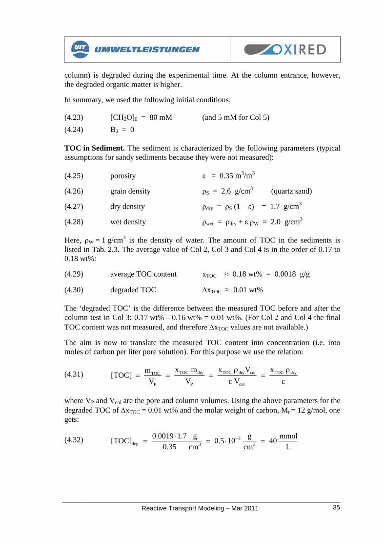
Input Waters. In the experiments, the inflow water was taken from Lake Tegel as dis-cussed in § 2.1. Based on the analyzed water composition (raw data) input waters for thereactive transport model has been generated by PHREEQC. These ‘synthetic’ waters arefree of charge-balance errors, IB = 0, and stay in equilibrium with mineral phases (see§ 3.3).
The so prepared water composition, exemplary for Col 5, is listed in Tab. 2.5. The in-flow waters (model input) of the other columns differ only slightly from these data.
Tab. 2.5 Inflow water of Col 5 (model input generatedwith PHREEQC).
inflow water Col 5 not ozonated ozonated
pH - 8.0 8.0
pe - 6.6 12.6
T °C 25 25
Ca mg/L 104 104
Mg mg/L 14.3 14.3
Na mg/L 39.5 39.5
K mg/L 6.6 6.6
S(6) mg/L 168 168
C(4) mg/L 36.4 36.4
Cl mg/L 54.9 54.9
Fe mg/L 210-9
210-9
Al mg/L 0.11 0.11
N(-3) mg/L 0 0
N(3) mg/L 0.88 0
N(5) mg/L 6.7 7.9
P mg/L 0.006 0.006
Si mg/L 0.11 0.11
F mg/L 0.4 0.4

Reactive Transport Modeling – Mar 2011 15
Inflow Regime. There are three types of inflow waters:
LT unprepared Lake Tegel water
LT_O3 ozonated Lake Tegel water
LT_tracer ozonated Lake Tegel water with 10 mg/L LiBr (see below)
During the experiments the inflow water changes according to a predefined time regime:
LT LT_O3 LT_tracer LT_O3 LT
The start and end times of each interval vary slightly from column to column. The spe-cific time regime of each column test (as defined in [TUB11]) was considered in TRNexplicitly.
Tab. 2.5 shows the composition of the non-ozonated and the ozonated water, LT andLT_O3. Both waters differ by the pe value (redox potential) and the N speciation (i.e.how N disproportionates into nitrate, nitrite, and ammonium). The relation between pevalue and redox potential Eh is defined in Eq. (4.6) and Eq. (4.7), respectively.
Remark. Ozonated water is not stable. The ozone (self-)decay was simulated by a modi-fication of the inflow waters.
Tracer. In all column tests LiBr was used as tracer. It has been injected with a uniformconcentration of
LiBr = 10 mg/L
The start time t1 and injection interval, t2 – t1, was different in each column test:
Col 2: t1 = 164 h t2 = 235 h (3 days)Col 3: t1 = 99 h t2 = 124 h (1 day)Col 4: t1 = 309 h t2 = 341 h (1⅓ day)Col 5: t1 = 98 h t2 = 125 h (1 day)
Initial Water. The initial water which enters each column cell at t = 0 was chosen as theunprepared Lake Tegel water, LT.
2.2.4 Thermodynamic Database
PHREEQC, which is embedded in the reactive transport model, uses the standard data-base wateq4f. For transparency reasons, this database is applied in its original form. Ad-ditional species that are not contained in wateq4f are added to the PHREEQC input filesas header (the same header for all PHREEQC calculations during running TRN). Thus,we never change or disturb the original database file ‘wateq4f.dat’.


Reactive Transport Modeling – Mar 2011 17
3 HYDRAULICS AND HYDROCHEMISTRY
3.1 Advection and Dispersion
The breakthrough of the tracer ‘LiBr’ was used to check and adjust the hydraulic pa-rameters. More precisely, only the anion Br- is the tracer per se whereas the cation Li+
undergoes ion exchange (see Fig. 3.1 and § 3.2).
Fig. 3.1 Calculated and measured breakthrough of Li+ and Br- in Col 2; model without and with ion exchange – bluecurves, experiment – red dots (screenshots of TRN).
An optimal description of bromide Br- was achieved (in all column tests) by the follow-ing parameter set:
volumetric flow Q = 1.0 to 1.3 mL/min (depends on column test)pore volume = 0.35longitudinal dispersivity L = 0.3 cm
These parameters are used in all calculations of the present study. The dispersivity L
enters the Advection-Dispersion equation via the longitudinal dispersion coefficient:
(3.1) vD LL
without Ion Exchange
Li
Br
Li
Br
with Ion Exchange

Reactive Transport Modeling – Mar 201118
Fig. 3.2 shows how an increase of the longitudinal dispersion L smoothes the bromidebreakthrough curves in Col 3. The simulation starts with pure advection, i.e. L = 0,where there is no smoothing at all (due to the fact that the model is free of numericaldispersion).
Fig. 3.2 Tracer ‘Bromi-de’ in Col 3 simulatedwith different longitudi-nal dispersions L (L =0 is pure advection).
3.2 Cation Exchange
Any natural sediment contains at least small amounts of clay or other minerals (ratherthan pure quartz SiO2). Clays give reason for ion exchange. Therefore, in all calcula-tions ion exchange of the cations H+, K+, Na+, Ca2+, Mg2+, Li+, and NH4
+ is taken intoaccount. They are defined by the following reactions (with log K values from wateq4f):
(3.2) H+ + X- = HX log K = 1.0
(3.3) K+ + X- = KX log K = 0.7
(3.4) Na+ + X- = NaX log K = 0.0
(3.5) Li+ + X- = LiX log K = -0.08
(3.6) Ca+2 + 2X- = CaX2 log K = 0.8
(3.7) Mg+2 + 2X- = MgX2 log K = 0.6
(3.8) NH4+ + X- = NH4X log K = 0.6
(3.9) Fe+2 + 2X- = FeX2 log K = 0.44
(3.10) Al+3 + 3X- = AlX3 log K = 0.36
Since the Fe and Al concentrations in the inflow solution are below the detection limition exchange of Fe+2 and Al+3 plays a minor role only. Nonetheless, these processes arenot excluded from calculations. Instead, it was assumed that the (very small) Fe and Alconcentrations are in equilibrium with FeOOH (goethite) and Al2Si2O5(OH)4 (kaolinite).
0
5
10
15
20
25
30
35
40
45
5 6 7 8 9 10 11
time [days]
Bro
mid
e[m
g/L
]
pure ADV
DISP = 0.3 cm
DISP = 0.6 cm
DISP = 1.2 cm

Reactive Transport Modeling – Mar 2011 19
CEC. Besides the thermodynamic data (log k values from wateq4f) the reactive trans-port model requires the input parameter ‘total cation capacity per pore volume’:
(3.11)
TOT
P
clay
P
sites)pore( C
V
mCEC
V
nC
TOT
where nsites is the number of exchanger sites in meq and VP is the pore volume. Thecation exchange capacity, CEC, of a typical (dry) clay mineral, such like Montmorillo-nite, is
(3.12)g100
meq90
m
nCEC
clay
sites
Assuming a low clay content of 1 wt%, that is, f = mclay/msed = 0.01 where msed is the drysediment mass with density ρB ≈ 1.7 g/cm3, we obtain as a first approximation
(3.13)L
meq15CECfC BTOT ‘theoretical value’
In the model calculations we used CTOT = 15 meq/L as the start value (prior to the com-parison with the experiment). The comparison of the calculated and measured break-through of Li+ was then used to adjust CTOT properly. In general, the higher CTOT thehigher is the retardation.
Results. The adjusted values of CTOT are the following (see Fig. 3.3):
Col 2: CTOT = 20 meq/LCol 3: CTOT = 20 meq/LCol 4: experimental data for Li+ violate mass balanceCol 5: CTOT = 5 meq/L (CEC shrinks due to 550°C treatment)
There is a good agreement between the rough ‘theoretical’ prediction in Eq. (3.13) andthe extracted CTOT values. Also, CTOT becomes smaller in the sediment pretreated with550 °C due to the temperature-driven artificial weathering. Col 5 shows a smaller retar-dation.
The experimental data of Col 4 (shown in the middle-left diagram of Fig. 3.3) are toosmall in comparison to the prediction (independent of any particular choice for CTOT).Here, the mass balance deficiency of approximately 50 %, calculated from the area be-neath the measured data points, remains an open question. The argument that Li+ isfixed by HFO complexes of the iron-coated sand is not supportable since such an HFO-effect is not seen in Col 5 that contains iron coated sand as well.

Reactive Transport Modeling – Mar 201120
Fig. 3.3 Calculated and measured breakthrough of Li+ in Col 3, Col 4, and Col 5; model with ion exchange – bluecurves, experiment – red dots (screenshots of TRN).
Tab. 3.1 Sorbed cations on ion exchanger (Col 4)
Fig. 3.4 Pie chart of sorbed cations on ionexchanger in Col 4 (data from Tab. 3.1).
IX speciesconcentration
[meq/L]
HX 910-5
KX 0.173
NaX 0.326
CaX2 17.18
MgX2 2.319
FeX2 ~ 0
AlX3 ~ 0
NH4X ~ 0
LiX ~ 0
CTOT 20.0
Q = 1.3 mL/min
Fe-coated /dried sediment 200°C
Fe-coated /heated sediment 550°C
Br Li
Br
Br
Li
Li
Li
Col 3
Col 4
Col 5
retarded ?adsorbed ?
LiLi
CTOT = 5 meq/L
dried sediment 200°C
Q = 1.0 mL/min
Q = 1.1 mL/min
CTOT = 20 meq/L
other
0%
NaX
2%
KX
1%HX
0%
MgX2
12%
CaX2
85%
HX
KX
NaX
CaX2
MgX2
other

Reactive Transport Modeling – Mar 2011 21
Tab. 3.1 shows the distribution of cations on the ion exchanger that is in equilibriumwith Lake Tegel water (without LiBr tracer). The partial concentrations sum up to thetotal exchange capacity CTOT = 20 meq/L. Please note that up to 85 % of the ion ex-changer is occupied by Ca.
Fig. 3.5 displays the outflow concen-trations of K, Mg, and Ca in Col 3. Kas a non-reactive element can only beinfluenced by ion exchange (like Li).Thus, the interesting behavior of K inthe upper diagram is caused by load-ing and deloading of the other majorions like Ca and Mg (Note: the Caconcentration is one order of magni-tude higher than the K concentration).The behavior of Ca is affected by pHand the mineral phase calcite as it willbe discussed in § 3.3.2.
Fig. 3.5 Outflow concentrations of K, Mg, and Cain Col 3 (model calculations and experiments).time [days]
K [mg/L]
Mg [mg/L]
Ca [mg/L]

Reactive Transport Modeling – Mar 201122
3.3 Mineral Phases
3.3.1 Theoretical Background
In principle, there are two possibilities to simulate the dissolution and precipitation ofminerals:
by kinetics (based on a kinetic approach and additional parameters) by thermodynamics (based on log k values contained in the PHREEQC database)
The advantage of the equilibrium approach is that it relies on fundamental thermody-namic data rather than on empirical kinetic data (which are less known and in mostcases not available).
Accordingly, it is quite useful to separate between reactive (or primary) and secondaryminerals:
reactive minerals (dissolution only) secondary minerals (precipitation and dissolution)
Reactive minerals act as a source; secondary minerals act mainly as a sink for elements.Therefore, reactive minerals require an initial mass m0 (more precisely: the initialamount n0 of moles per liter solution). Whereas reactive minerals are predestinated for akinetic approach secondary minerals are described as reversible processes controlled byequilibrium thermodynamics.
Thought the separation between reactive and secondary minerals is very convenient forconceptual models, in natural systems there is no such sharp borderline. Typical reactiveminerals are pyrite, clay minerals and carbonates (calcite, dolomite); typical secondaryminerals are gypsum, amorphous hydroxides like Fe(OH)3 and Al(OH)3, and calcite.Thus, calcite can be assigned as a reactive or a secondary mineral. In the present studywe use a kinetic approach for calcite – see Eqs. (3.18) and (3.19).
IAP and SI. The dissolution and precipitation of a mineral phase, AB, is given by thereaction formula
(3.14) mineral A + B
For example, in case of calcite, CaCO3, A and B symbolize Ca+2 and CO3-2. The activi-
ties of reactants A and B at equilibrium defines the equilibrium constant
(3.15) eqeq ]B[]A[K (equilibrium constant)
On the other hand, the measured activities define the ion activity product
(3.16) actualactual ]B[]A[IAP (ion activity product)
dissolution
precipitation

Reactive Transport Modeling – Mar 2011 23
The saturation index is then defined by
(3.17)
K
IAPlogSI (saturation index)
According to the SI value we distinguish between three cases:
SI = 0 solution is saturated with the mineralSI < 0 solution is under-saturated with the mineralSI > 0 solution is supersaturated with the mineral
If SI < 0 we have IAP < K and the reaction in Eq. (3.14) will proceed to the right (disso-lution). Vice versa, if SI > 0 we have IAP > K and the reaction will proceed to the left(precipitation).
3.3.2 Model Calculations
With regard to ‘reactive minerals’ the columns represent a simple system. The sedimentused in the experiments is in equilibrium with the solution (lake water) and long-termweathering processes do not need to be considered in these short-term tests. Thereforeno ‘primary minerals’ are considered in the model. However, ‘secondary minerals’ thatcould precipitate from the solution have been included in all calculations:
gypsum CaSO4H2O ferrihydrite Fe(OH)3
aluminum hydroxide Al(OH)3
amorphous SiO2 SiO2(am) calcite CaCO3 as kinetic reaction
From these minerals only calcite affects the water composition significantly (see Fig. 3.6);calcite is treated as a kinetic reaction. The other minerals enter the model as ‘equilib-rium phases’ based on log k values (taken from the PHREEQC’s standard databasewateq4f). However, the influence of these equilibrium phases is negligible in the columntests; only small amounts (if any) precipitate.
Fig. 3.6 Ca and DIC in the outflow solution in Col 3 (model calculations and experiments).
as equilibrium phases
time [days] time [days]
Ca [mg/L]DIC [mg/L]

Reactive Transport Modeling – Mar 201124
The extraordinary role of calcite already becomes clear from the hydrochemistry of theinflow water from Lake Tegel: This water is supersaturated with calcite, what calls for akinetic description.
Calcite Kinetics. The dissolution and precipitation of calcite is treated as ‘higher-orderkinetics’ depending on the saturation index, SI (see also Eq. (A.12), [PA99]):
(3.18)
0
SIdiss
diss m
m101r
dt
dm
V
1for SI < 0
(3.19) SIprec
prec
101rdt
dm
V
1 for SI > 0
Here, m(t) and m0 denote the actual and initial amount of calcite in mol; V is the solu-tion volume, and rdiss and rprec are the specific dissolution and precipitation rates:
rdiss = 310-8 mol/L/srprec = 110-8 mol/L/s
The initial amount of calcite, m0, was fitted to the data (see Tab. 3.2). It represents thereactive fraction of the total CaCO3 in the sediment, i.e. that part that is in direct contactto the solution. Please note that the precipitation does not depend on the calcite amountm or m0.
Initial Acidity. In all column tests a wash-out of ‘weathering products’ was observedjust after start. This effect is accompanied (except Col 5) with a steep decrease of pHfrom about 8.5 to 6 (see red dots in Fig. 3.7). This relatively fast ‘acidification’ cannotbe explained neither by mineral dissolution nor by biodegradation alone. It seems to bean artificial effect caused by the pre-treatment/heating of the sediment (weathering of thematerial due to air contact). In order to simulate this effect we assume a short-termacidification by acids, abbreviated by ‘HA’, that generate H+ ions with decreasing ratefrom 10-7 mol/L/s to zero in the first 20 hours (first-order kinetics with an initial amountgiven in Tab. 3.2).
Fig. 3.7 pH value in the outflow solution inCol 3 (model calculations and experiments).
pH
time [days]

Reactive Transport Modeling – Mar 2011 25
Results. Comparison of model calculations with measured data in Fig. 3.6 and Fig. 3.7shows the sensitive interrelation between pH, Ca, and DIC (dissolved inorganic carbon)in the outflow solution of Col 3. In particular, small changes of pH strongly affect bothCa and DIC concentrations, and vice versa.
This behavior is typical for all columns but it is best evidenced in Col 3. In Col 2 the Cavalues and in Col 4 the DIC values are missing in the time interval just after start. OnlyCol 5 behaves completely different due to the severe pre-treatment at 550 °C.
Initial Conditions. The pre-treatment of the sediment differs from column to column(as indicated in Tab. 2.1). Particularly this variation reflects in the initial amounts ofcalcite and HA as shown in Tab. 3.2. These parameters are not known beforehand; theywere adjusted in model calculations.
Tab. 3.2 Initial amount of calcite and acidity (HA) in mmolper liter pore solution.
The data in Tab. 3.2 indicate that the amount of calcite in Col 2 (untreated sediment) issmaller than in Col 3 and Col 4. On the other hand, in Col 5 calcite seems to be de-stroyed by the pre-treatment at 550 °C. The same considerations are valid for the initialacidity potential (HA).
Final Note: Hydrochemical modeling does not allow separate adjustment of one pa-rameter (i.e. element) without influencing all other parameters. All quantities are tightlyconnected with each other by mass balance and by charge balance.
initialamount
Calcite[mM]
HA[mM]
Col 2 1 4
Col 3 5 8
Col 4 5 8
Col 5 0 0

Reactive Transport Modeling – Mar 201126
3.3.3 Comparison of three Calcite-Precipitation Models
Three precipitation models for calcite are compared:
kinetic approach (applied and described in § 3.3.2) equilibrium approach (based on thermodynamic log K values) no calcite / no precipitation
In the equilibrium approachsuper-saturation of SI = 0.5is assumed.
The results are shown inFig. 3.8. The diagrams dis-play pH, Ca, and DIC in theoutflow solution of Col 3(experimental data are mar-ked by red dots). Evidently,the best description is ob-tained by the kinetic ap-proach (blue curve).
Fig. 3.8 Comparison of three “calciteprecipitation models”: (i) kinetic ap-proach, (ii) equilibrium thermodynam-ics, (iii) no calcite / no precipitation.The diagrams show are pH, Ca, andDIC in the outflow solution of Col 3(dots – experimental data).
3
4
5
6
7
8
9
0 1 2 3 4 5 6 7 8 9 10 11 12
pH
va
lue
pH
Calc_kin
Calc_eq
Calc_no
0
20
40
60
80
100
120
140
160
180
200
0 1 2 3 4 5 6 7 8 9 10 11 12
Ca
[mg
/L]
Ca
Calc_kin
Calc_eq
Calc_no
0
10
20
30
40
50
60
70
80
0 1 2 3 4 5 6 7 8 9 10 11 12
time [days]
DIC
[mg
/L]
DIC
Calc_kin
Calc_eq
Calc_no

Reactive Transport Modeling – Mar 2011 27
4 REDOX REACTIONS
4.1 Theoretical Background
Redox reactions are oxidation-reduction reactions. The term oxidation refers to the re-moval of electrons from an atom, forcing an increase in the oxidation number; reductionrefers to the addition of electrons to lower the oxidation number. Thus, in redox reac-tions there is always a transfer of electrons from a reducing agent ‘Red’ (electron donor)to an oxidizing agent ‘Ox’ (electron acceptor):
(4.1) 11 dReneOx (reduction)
(4.2) neOxdRe 22 (oxidation)
which add up to the total reaction equation
(4.3) 2121 OxdRedReOx
Here n denotes the number of electrons. The electron exchange occurs between so-called redox-sensitive elements, i.e. elements with more than one valence state (oxida-tion number): C, O, N, S, Fe, Mn, and other trace metals like Mo, Cr, As, Co, Ni, Sb, Thand U. Free electrons do not exist in natural systems, hence, any group of half reactionswhich add up to the total reaction equation should obey the ‘electron balance’.
Redox reactions are mediated by microorganisms. The microorganisms act as catalystsspeeding up the reactions that otherwise would be extremely slow. The electron transfermediated by microbes is sketched in Fig. 4.1.
Fig. 4.1 Electron trans-fer in redox reactionsmediated by microor-ganisms.
Microbe
e-D
on
or
e-A
ccep
tor
Ox Ox + e-
Red + e- Red
e- Energy(ATP)
+
oxidation (loss of e-)
reduction (gain of e-)
half reactions
Reactive Transport Modeling – Mar 201128
Half-redox reactions are similar to other equilibrium reactions. (Please note that theabove equations are analogous to acid-base reactions where instead of an electron trans-fer there is a transfer of protons, H+.) Thus, in parallel to the definition of pH there is asimilar definition of pe based on the ‘electron concentration’ or ‘electron activity’ [e-]:
(4.4) ]H[logpH
(4.5) ]e[logpe
High proton concentration means low pH-values; high ‘electron concentration’ meanslow pe-values. The relation between the measured redox potential or ORP in V relativeto SHE (standard hydrogen electrode), and the pe-value is
(4.6) hERT10ln
Fpe
where the FARADAY constant is F = 96 490 JV-1 and R = 8.314 Jmol-1K-1. For 25 °C(T = 298.15 K) the equation simplifies to
(4.7) 059.0/]V[Epe h
If some of the half-redox reactions are in equilibrium, redox phenomena can be modeledas equilibrium processes (using PHREEQC-code, for example). However, redox reactionsoften are slow relative to physical processes (transport, mixing etc.) which call for akinetic description.
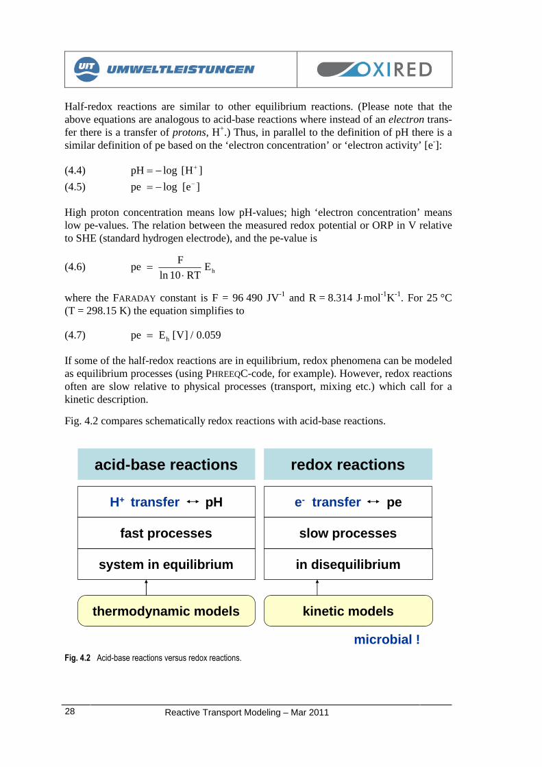
Fig. 4.2 compares schematically redox reactions with acid-base reactions.
Fig. 4.2 Acid-base reactions versus redox reactions.
acid-base reactions
H+ transfer pH e- transfer pe
redox reactions
fast processes slow processes
system in equilibrium in disequilibrium
thermodynamic models kinetic models
microbial !

Reactive Transport Modeling – Mar 2011 29
4.2 Experimental Evidence for Redox Reactions
Redox reactions are, in fact, the central topic of the present OXIRED 2 project. In natu-ral systems redox reactions are mediated by microbial activity [KWB10]. In particular,aerobic biodegradation of organic material results in a decrease of the redox potential(Eh or pe value) and pH value. These effects are seen in the column experiments.
Fig. 4.3 Measured redox potential, Eh or pe, in Col 2 to Col 5.
Fig. 4.3 displays the measured redox potential in the outflow solution of Col 2 to Col 5.After starting the column tests the redox potential drops down from pe ≈ 10 to -4 inCol 2 and Col 3, and from pe ≈ 13 to -2.5 in Col 4 which is an indicator for microbialactivity.
Conversely, there is no evidence for microbial activity in Col 5 (the redox potential re-mains at ambient oxic conditions at pe ≈ 5). It seems quite reasonable that the microbialpopulation was damaged during the pre-treating of the sediment at 550 °C. Only Col 5was pretreated at such high temperatures (see Tab. 4.1).
Tab. 4.1 Column setup used in the experiments.
Col 1 Col 2 Col 3 Col 4 Col 5
flow Q mL/min 1.3 1.3 1.0 1.1
sediment natural natural 200 °C 200 °C 550 °C
CEC meq/L 20 20 20 20 5
µ biology yes yes yes yes no
Fe-coated sand no no no yes yes
-5,0
-2,5
0,0
2,5
5,0
7,5
10,0
12,5
15,0
0 2 4 6 8 10 12 14 16 18 20
Time in days
pE
-300
-150
0
150
300
450
600
750
900
Eh
inm
V
Col 2
Col 3
Col 4
Col 5
microbial activity (Col 2 to 4)
no microbial activity (Col 5)

Reactive Transport Modeling – Mar 201130
4.3 Redox Sequences in the Column Tests
Sequences of redox reactions and redox zoning play a key role in environmental geo-chemistry [AP05] and, especially, in bank filtration and artificial recharge [KWB10].Fig. 4.4 displays typical redox sequences at neutral pH. The diagram highlights the halfreactions (in orange color) which are relevant for biodegradation in the present columntests. In particular, the system does not contain sufficient manganese and dissolved ironto be relevant.
Fig. 4.4 Redox sequences at pH = 7 in natural systems. Half-reactions which are relevant for the biodegradation inthe present column tests are marked in orange color.
e- Donor. All columns contain organic matter (as it is evident from the measured fOC
values in Tab. 2.3). Thus, the starting point for all further consideration is the biodegra-dation of organic matter. It is a good approximation to use CH2O (i.e. 1/6 glucose) as acommon representative for organic matter. In this way, CH2O acts as electron donor inthe oxidation half-reaction:
(4.8) CH2O + H2O = CO2 + 4H+ + 4e- oxidation: C(0) C(IV)
0 10 20-20 -10
0 10 20-20 -10
O2 reduction
denitrification
MnO2 → Mn+2
Fe(3) oxide → Fe+2
SO4-2 reduction
CH4 fermentation
reductions
oxidation of Corg
Sulfide → SO4-2
Fe+2 oxidation
nitrification
Mn+2 oxidation
oxidations
pe
half-reactions relevant inCol 2, Col 3, and Col 4

Reactive Transport Modeling – Mar 2011 31
e- Acceptors. There are four potential e- acceptors in the column system: oxygen, ni-trate, nitrite, and sulfate. The corresponding reduction half-reactions are:
(4.9) O2 + 4H+ + 4e- = 2H2O reduction: O(-II) O(0)
(4.10) NO3- + 2H+ + 2e- = NO2
- + H2O reduction: N(V) N(III)
(4.11) NO2- + 8H+ + 6e- = NH4
+ + H2O reduction: N(III) N(-III)
(4.12) SO4-2 + 10H+ + 8e- = H2S + 4H2O reduction: S(VI) S(-II)
In reality, the reaction pathways are not nearly as simple as considered. For example, thereduction of nitrate to ammonium proceeds via several nitrogen compounds:
(4.13) NO3- NO2
- NOx N2 PON DON NH4+
Here, NOx abbreviates the gases NO, NO2, N2O; PON and DON are particular organicnitrogen and dissolved organic nitrogen.
The same holds true for sulfate which is reduced in long chain of steps down to sulfide,S(-II), where in total eight electrons are transferred:
(4.14) SO4-2 SO3
-2 S2O3-2 S S-2 HS- H2S
For example, the reduction to sulfite is given by
(4.15) SO4-2 + 2H+ + 2e- = SO3
-2 + H2O reduction: S(VI) S(IV)
Note: The ‘sulfite chemistry’ defined in Eq. (4.15) is not contained in wateq4f. Thus, weexplicitly implemented the ‘sulfite chemistry’ into the model to study this effect.
As it will be shown in the model calculations in § 4.5 the redox processes in the col-umns are dominated by the major electron acceptors O2, nitrate and nitrite alone. Thesulfate reduction is too small to be reliable identified by the experimental data (even ifthe ‘sulfite chemistry’ defined in Eq. (4.15) is considered). Images of redox zonationinside the column are given in Fig. 4.13.
4.4 Biodegradation and Enzyme Kinetics
4.4.1 Conceptual Model
The biodegradation model bases on a combined approach of enzyme kinetics and ther-modynamics. Whereas the degradation of organic matter in Eq. (4.8) is treated by en-zyme kinetics the accompanied electron transfer and electron balance is controlled bythermodynamics (using PHREEQC). In PHREEQC all relevant redox reactions are consid-ered per se; they are defined in the thermodynamic database (wateq4f) which contains along list of reaction equations and log K values (equilibrium constants).

Reactive Transport Modeling – Mar 201132
Enzyme Kinetics. A brief introduction to enzyme kinetics is presented in Appendix B.The set of differential equations that considers both enzyme kinetics and populationdynamics is given in Eqs. (B.20) to (B.22):
(4.16) )t(BY
)t(
dt
]S[d
(4.17) )t(B)t(dt
dB
(4.18)]S[K
]S[)t(
S
max
Here, the symbols are:
[S(t)] substrate concentration in mol/LB(t) biomass concentration in cells/LKS half-saturation constant in mol/Lµmax maximum rate in 1/s cell death rate in 1/sY yield coefficient in cells/mol
This submodel contains at least four parameters which are not known beforehand: µmax,KS, and Y (as well as the initial biomass concentration B0). The number of experi-ments, however, is too small in order to fit all these parameters reliably. Hence, somesimplifications will be done below.
The enzyme kinetics is applied for the oxidation of organic matter defined in Eq. (4.8),i.e. the substrate is CH2O. Inserting Eq. (4.18) into Eq. (4.16) we get
(4.19)
max2S
20
2
B
)t(B
]OCH[K
]OCH[
dt
]OCH[dwith max
max0 B
Y
Population Dynamics. The population dynamics, B(t), is used to simulate the lagtimebehavior of the microorganisms (at t = 0 it starts with B0 ≈ 0). Instead of solving thedifferential equation (4.17) numerically (whereby is an unknown parameter) we use ananalytical closed-form expression. It is assumed that the active biomass grows from zeroto a saturation level Bmax according to a smooth step function:
(4.20)
1
lag
max
ttexp1
B
)t(B
where tlag is the lagtime and a smoothing parameter. As shown in Fig. 4.5 this ‘nor-malized’ function starts at zero and switches to 1 when the time comes near the lag time,t ≈ tlag. The parameter controls how steep or smooth the transition from 0 to 1 is (thelarger the broader the transition).

Reactive Transport Modeling – Mar 2011 33
Fig. 4.5 Populationdynamics in Col 2 andCol 4 expressed by the‘normalized’ biomassconcentration B(t)/Bmax
in Eq. (4.20).
e Acceptors. So far Eq. (4.19) works for conditions where the supply of electron accep-tors in the system is time-independent. In practice, however, the amount of e-acceptors(oxygen, nitrate, and nitrite) varies strongly over time. The higher the amount of e-acceptors the faster the organic material degrades (no e-acceptors – no degradation).Thus, it is assumed that the biodegradation rate is proportional to the amount of all e-acceptors actually present in the system, especially O2(t), NO3
-(t) and NO2-(t). Mathe-
matically, the constant rate parameter µ0 in Eq. (4.19) is replaced by a time-dependentone:
(4.21) µ0 )t(f)t( accepteff0
with
(4.22) )t(NOa)t(NOa)t(Oaf)t(f 2231200accept
Here, the coefficients are chosen as a0 = a1 = 1 mol-1 and a2 = ½ a1. In addition, the tiny‘background factor’ f0 = 110-5 accounts for all other minor e-acceptors in the columnsystem (sulfate, redox specific metal ions, etc.). The ai coefficients are chosen as 1.
[Note: In the experiments O2 is always accompanied with nitrate. Thus, in order to keepthe parameter number as small as possible O2 and NO3
- are lumped together into oneterm of Eq. (4.22).]
Eq. (4.19) with µ0(t) is used to calculate at each time step ti and in each column cell xn
the amount m of CH2O that is biodegraded. The electrons released in this oxidationreaction are captured by electron acceptors like O2, nitrate and/or nitrite (which undergoa reduction process).
0,0
0,1
0,2
0,3
0,4
0,5
0,6
0,7
0,8
0,9
1,0
1,1
0 2 4 6 8 10 12 14 16 18 20
time [days]
bio
mass
(norm
aliz
ed)
Col 2
Col 4
t_lag (Col 2) t_lag (Col 4)

Reactive Transport Modeling – Mar 201134
4.4.2 Model Parameters and Initial Conditions
Parameter Adjustment. The biodegradation model defined by Eqs. (4.19) to (4.21)contains four main parameters:
µeff effective rate in mol/L/sKS half-saturation constant in mol/Ltlag lag time in h time parameter in h
These four parameters were adjusted to get an optimal description of the time develop-ment of 7 measured quantities: pe value, dissolved oxygen, nitrate, nitrite, ammonium,as well as pH and DIC. The so obtained ‘best-fit’ parameter set is listed in Tab. 4.2.
Tab. 4.2 Parameter set for enzyme kinetics (extracted from column tests)
As discussed in § 4.2, microbial activity is expected in Col 2, Col 3, and Col 4, but it isdamaged in Col 5 due to the heating of sediment at 550 °C. Nonetheless, Col 5 was notexcluded from the redox calculations; the extracted parameter set for Col 5, however,may be not very meaningful. The major premise in performing the parameter fit was thatthe two MICHAELIS-MENTEN parameters µ0 and KS should be equal in all ‘microbialactive’ columns, i.e. in Col 2, Col 3, and Col 4. This was, in fact, achieved as shown inTab. 4.2.
Initial Conditions. In addition to the four model parameter the two differential equa-tions (4.19) and (4.20) require two initial conditions for t = 0:
[CH2O]0 initial mass of reactive CH2O in mol/LB0 = 0 initial biomass in mol/L
An estimation for the initial organic matter which is accessible and degradable by mi-croorganisms [CH2O]0, follows from the measured TOC in the sediment (before andafter the column test). As shown below, the maximum degraded TOC is in the order of40 mM carbon (result of measurement at the column entrance, but keep in mind themeasure accuracy). The degradable TOC inside the columns should be larger than thisvalue. In particular, assuming an initial mass [CH2O]0 of, say, 80 mM we observed inthe calculations that only a small amount (of about 5 % as an average over the whole
µeff KS t_lag column
sediment(preparation) mol/L/s mmol/L hours hours
Col 2 natural 410-7 8 72 12
Col 3 200 °C 410-7 8 36 18
Col 4 200 °C 410-7 8 96 18
Col 5 550 °C 0.410-7 0.05 4 3
Reactive Transport Modeling – Mar 2011 35
column) is degraded during the experimental time. At the column entrance, however,the degraded organic matter is higher.
In summary, we used the following initial conditions:
(4.23) [CH2O]0 = 80 mM (and 5 mM for Col 5)
(4.24) B0 = 0
TOC in Sediment. The sediment is characterized by the following parameters (typicalassumptions for sandy sediments because they were not measured):
(4.25) porosity ε = 0.35 m3/m3
(4.26) grain density ρS = 2.6 g/cm3 (quartz sand)
(4.27) dry density ρdry = ρS (1 – ε) = 1.7 g/cm3
(4.28) wet density ρwet = ρdry + ε ρW = 2.0 g/cm3
Here, ρW = 1 g/cm3 is the density of water. The amount of TOC in the sediments islisted in Tab. 2.3. The average value of Col 2, Col 3 and Col 4 is in the order of 0.17 to0.18 wt%:
(4.29) average TOC content xTOC ≈ 0.18 wt% = 0.0018 g/g
(4.30) degraded TOC xTOC ≈ 0.01 wt%
The ‘degraded TOC’ is the difference between the measured TOC before and after thecolumn test in Col 3: 0.17 wt% – 0.16 wt% = 0.01 wt%. (For Col 2 and Col 4 the finalTOC content was not measured, and therefore xTOC values are not available.)
The aim is now to translate the measured TOC content into concentration (i.e. intomoles of carbon per liter pore solution). For this purpose we use the relation:
(4.31)
dryTOC
col
coldryTOC
P
dryTOC
P
TOCx
V
Vx
V
mx
V
m]TOC[
where VP and Vcol are the pore and column volumes. Using the above parameters for thedegraded TOC of xTOC = 0.01 wt% and the molar weight of carbon, Mr = 12 g/mol, onegets:
(4.32)L
mmol40
cm
g105.0
cm
g
35.0
7.10019.0]TOC[
3
3
3deg

Reactive Transport Modeling – Mar 201136
Thermodynamics & Kinetics. Fig. 4.6 sketches the idea behind the interplay of ther-modynamics and kinetics in the applied model. The biodegradation of CH2O is simu-lated by enzyme kinetics. Each molecule of CH2O releases 4 electrons which are imme-diately captured by e- acceptors (O2, NO3
-, NO2-). The latter process is completely con-
trolled by thermodynamics (where the reaction stoichiometry and log K values are de-fined in the PHREEQC database wateq4f). The so modified concentrations of the redoxspecies (e- acceptors) influence then, via the rate coefficient μ0(t), the degradation proc-ess. In this way, the system represents a nonlinear feedback loop.
Fig. 4.6 Interplay of thermodynamics and kinetics in the present model: Nonlinear feedback loop connected byelectron balance.
electron flow
max2S
20
2
B
)t(B
]OCH[K
]OCH[
dt
]OCH[dmax
maxeff B
Y
)t(f)t( accepteff0
)t(NOa)t(NOa)t(Oaf)t(f 2231200accept
A non-linear system.
Th
erm
od
yn
am
ics
Enzyme Kinetics

Reactive Transport Modeling – Mar 2011 37
4.5 Application and Model Results
4.5.1 Model Calculations versus Experiments
The simulation of the redox processes is based on the biodegradation model inEqs. (4.19) to (4.21) and the parameter set in Tab. 4.2. In the following we focus on thepe value (ORP) and the redox species:
dissolved oxygen O(0) nitrate N(5) nitrite N(3) ammonium N(-3)
[All other elements are already discussed in the foregoing Chapters.] The measured andcalculated outflow concentrations of these four redox species are shown in the diagramsof Fig. 4.7 (for Col 2), in Fig. 4.8 (for Col 3), in Fig. 4.9 (for Col 4), and in Fig. 4.10(for Col 5). In addition, pH ant the pe values for all columns are displayed in Fig. 4.11.In all cases the model fits the general trend of the experimental data.
From the mathematical point of view, the underlying system is highly non-linear. Justsmall changes of one single element concentration cause huge changes of the pe value.This effect is observable, for example, in the pe diagrams of Fig. 4.11. In this way, thenumerical simulation of redox reactions belongs to the most complicated tasks in hydro-chemistry. In order to understand the ongoing processes (and to avoid misinterpretation)50 to 80 test calculations for each column were performed (in total about 350 calcula-tions).
The benefit of this study is that we can now ‘visualize’ and quantify the ongoing redoxprocesses inside each column as a function of time t and distance x. Processes that areunseen in the experiments are become uncovered now. Please note that the measureddata for the two N-species, nitrite and ammonium, are very sparse. This experimentalinformation alone is insufficient to draw any picture of redox zonation. Only the combi-nation of experiment and model calculation provides an adequate understanding of thecomplex dynamics (as it will be done in the next paragraph).

Reactive Transport Modeling – Mar 201138
Fig. 4.7 Oxygen, nitrate, nitrite, and ammonium in the outflow solution of Col 2 as a function of time (model calcula-tions and experiments; for nitrate and ammonium experimental data do not exist).
Fig. 4.8 Oxygen, nitrate, nitrite, and ammonium in the outflow solution of Col 3 as a function of time (model calcula-tions and experiments).
time [days] time [days]
Oxygen [mg/L] Nitrate [mg/L]
Nitrite [mg/L]Ammonium [mg/L]
Col 2
time [days] time [days]
Oxygen [mg/L] Nitrate [mg/L]
Nitrite [mg/L]Ammonium [mg/L]
Col 3

Reactive Transport Modeling – Mar 2011 39
Fig. 4.9 Oxygen, nitrate, nitrite, and ammonium in the outflow solution of Col 4 as a function of time (model calcula-tions and experiments).
Fig. 4.10 Oxygen, nitrate, nitrite, and ammonium in the outflow solution of Col 5 as a function of time (model calcula-tions and experiments).
time [days] time [days]
Nitrite [mg/L]Ammonium [mg/L]
Oxygen [mg/L] Nitrate [mg/L]Col 4
time [days] time [days]
Nitrite [mg/L]
Ammonium [mg/L]
Oxygen [mg/L]
Nitrate [mg/L]Col 5

Reactive Transport Modeling – Mar 201140
Fig. 4.11 pH and pe values in the outflow solution of Col 2 to Col 5 as a function of time (model calculations andexperiments).
time [days] time [days]
Col 2 Col 2
Col 3 Col 3
Col 4 Col 4
Col 5
Col 5
pH pe
pH pe
pH pe
pH
pe

Reactive Transport Modeling – Mar 2011 41
4.5.2 Interpretation – Redox Zonation inside Columns
The dynamics of the ongoing redox processes in time and space is illustrated inFig. 4.12 and Fig. 4.13. Fig. 4.12 shows the concentration of O2 and three N species inthe outflow solution of Col 3 as a function of time. Please note how oxygen, nitrate,nitrite, and ammonium seep out the column one after the other. Once O2 is depleted ni-trate transforms into nitrite; then nitrite transforms into ammonium so that after about 3days ammonium remains as the only N-species in the outflow solution. The steady stateis achieved after 7-8 days where the mass balance is fulfilled:
inflow concentration of NO3- = outflow concentration of NH4
+ = 0.1 mM
Ammonium, NH4+, as the only cation of all four redox species is absorbed on the ion
exchanger. Therefore, in contrast to the other three species with a sharp breakthrough,the ammonium curve is retarded (smoothed). The loading on the ion exchanger occursduring the first 5 days. After this time ammonium reaches the saturation value of0.1 mM in the outflow.
Fig. 4.12 Oxygen, nitrate, nitrite, and ammo-nium in the outflow solution of Col 3 as a func-tion of time.
Redox Zonation. The forming of redox zones inside Col 3 is shown in Fig. 4.13 at fourdifferent times. At the beginning (upper diagram) the column is filled with O2- and ni-trate-rich water (no zonation). This oxidized water is injected into the column and main-tains oxidizing conditions at the column inlet (first column cells near x ≈ 0). When timepasses biodegradation establishes reductive condition inside the column (about 5 cmaway from the entrance, and especially at the column outlet). After 20 hours (2nd dia-gram) nitrite is produced inside the column; after 45 hours (3rd diagram) ammoniumappears. At the same time O2 is depleted completely. The last diagram (after 70 hours)shows that the reductive conditions once established will prevail as a ‘steady state’ untilthe entire organic material is degraded (which, however, would require longer experi-mental time).
0,00
0,02
0,04
0,06
0,08
0,10
0,12
0,14
0,16
0 1 2 3 4 5 6 7 8
time [days]
Oxygen [mM]
Nitrate [mM]
Nitrite [mM]
Ammonium [mM]

Reactive Transport Modeling – Mar 201142
Fig. 4.13 Redox zonation within Col 3 atdifferent times (initial state in upper dia-gram)
0,00
0,02
0,04
0,06
0,08
0,10
0,12
0,14
0,16
0,18
0,00 0,05 0,10 0,15 0,20 0,25 0,30 0,35
Nitrate [mM]
Nitrite [mM]
Ammonium [mM]
Oxygen [mM]initial state
0,00
0,02
0,04
0,06
0,08
0,10
0,12
0,14
0,00 0,05 0,10 0,15 0,20 0,25 0,30 0,35
after 20 hours
0,00
0,02
0,04
0,06
0,08
0,10
0,12
0,00 0,05 0,10 0,15 0,20 0,25 0,30 0,35
after 45 hours
0,00
0,02
0,04
0,06
0,08
0,10
0,12
0,00 0,05 0,10 0,15 0,20 0,25 0,30 0,35
distance inside the column [m]
Nitrate [mM]
Nitrite [mM]
Ammonium [mM]
Oxygen [mM]
after 70 hours

Reactive Transport Modeling – Mar 2011 43
4.5.3 Limits and Benefits
Limits. The model represents a first approach to the complex branch of redox processes.Thus, we focused on three N species: nitrate, nitrite, and ammonium (the only concen-trations that are measured):
(4.33) NO3- NO2
- NOx N2 PON DON NH4+
The formation of N2 gas is not considered yet. However, in contrast to bioreactors (as‘open systems’) aquifer and columns represent ‘closed systems’ where gas formation ismore or less constraint. The good description of both pe value and ammonium justifythe chosen approach.
[Note: Probably two effects (not considered in the model) compensate each other: Theformation of additional ammonium during degradation of organic matter and the deple-tion of ammonium due to escape of N2.]
Model & Experiments. The present WP 3 demonstrates a sound combination of ‘ex-periment’ and ‘theory’. Due to this combination we are able to reveal details about theredox system that we didn’t think beforehand (looking on raw data alone).
Outlook. Once a model is calibrate by real data it can be used as a predictive tool forscenario simulations:
variation of flow velocity and other hydraulic/geometric parameters multi-layer systems with natural sediments and/or technical sand long-term experiments ( 3 month) larger columns (upscaling) column systems (including reactors)
The extension and upgrade of the model is an ongoing process (based on site- and pro-ject-specific data and knowledge). In this way, the model is ready to incorporate newaspects of geochemistry and geomicrobiology.
not measured


Reactive Transport Modeling – Mar 2011 45
5 SUMMARY
The present report belongs to Work Package 3 “Redox Control and Optimization at ARPonds” of the OXIRED 2 project started in January 2010. Work Package 3 consists oftwo main parts and was performed in cooperation with TUB:
Part I. Laboratory column experiments with special emphasis on sediment char-acteristics (by TUB)
Part II Numerical modeling of the results of the TUB column experiments (byUIT; present report)
The present report focuses on the geochemical interpretation of the TUB column ex-periments. A reactive transport model TRN – based on the U.S.G.S. code PHREEQC –was used to simulate four column tests (Col 2, Col 3, Col 4, and Col 5). The study wasperformed in several steps, from the simplest to the most complicated one:
hydraulics (advection & dispersion) in § 3.1 cation exchange in § 3.2 mineral phases (calcite kinetics) in § 3.3 redox reactions and biodegradation in Chapter 4
The system is highly dynamic. The aim was to combine all these separate processes intoa coherent whole that explains the formation of redox zones inside the columns (as afunction of time and column depth).
Hydraulics. The study starts with the adjustment of the hydraulic and geometric para-meter set for each column. This was done by fitting the breakthrough curve of bromide(resulting from added LiBr to the inflow solution). Whereas the anion Br- acts as perfecttracer the cation Li+ undergoes ion exchange.
Ion Exchange. The breakthrough of Li+ was used to extract the ion-exchange capacityCEC of the sediment. The deduced CEC of 20 meq/L agrees well with theoretical esti-mations for the sediment in Col 2 to Col 4. In Col 5, however, the sediment was pre-treated at 550 °C causing a temperature-driven artificial weathering which results in asmaller CEC of 5 meq/L.
Ion exchange is crucial to understand the behavior of other cations, especially K+, Mg+2,NH4
+ (as well as the retardation of carbamazepine). K+ as a non-reactive element is onlyinfluenced by ion exchange (like Li+). The good agreement between the calculated andobserved concentrations in Fig. 3.5 reflects the quality of the ion-exchange model(where the time-dependent behavior of K+ is caused solely by loading and deloading ofthe competing ions like Ca and Mg).

Reactive Transport Modeling – Mar 201146
Mineral Dissolution. The only mineral that significantly influences the column systemis calcite. The extraordinary role of calcite already becomes clear from the hydrochemis-try of the inflow water from Lake Tegel. This water is super-saturated with calcite, whatcalls for a kinetic approach (instead of pure equilibrium thermodynamics). The calcitedissolution rate was adjusted to describe the outflow concentrations of Ca, DIC, and pHvalue.
Redox Reactions. Redox reactions are the central part of the present study. For thispurpose a biodegradation model was established (and included into the reactive trans-port model). The biodegradation model bases on a combined approach of enzyme kinet-ics and thermodynamics. Whereas the degradation of organic matter in Eq. (4.8) istreated by enzyme kinetics the accompanied electron transfer and electron balance iscontrolled by thermodynamics (using PHREEQC). In PHREEQC all relevant redox reac-tions are considered per se; they are defined in the thermodynamic database (wateq4f)which contains a long list of reaction equations (stoichiometry) and log K values (equi-librium constants).
From the mathematical point of view, the redox system is highly non-linear. Just smallchanges of one single element concentration cause huge changes of the pe value. Thiseffect is observable, for example, in the pe diagrams of Fig. 4.11. In this way, the nu-merical simulation of redox reactions belongs to the most complicated tasks in hydro-chemistry. In order to understand the ongoing processes (and to avoid misinterpretation)50 to 80 test calculations for each column were performed (in total about 350 calcula-tions).
Redox Zonation. The benefit of the biodegradation model is that now we can quantifythe ongoing redox processes inside each column as a function of time and column depth.Processes that are unseen in the experiments are become uncovered now, especially thetransition from nitrate to nitrite to ammonium (despite the very sparse experimental datafor nitrite and ammonium). In this case, only the combination of experiment and modelcalculation provides an adequate understanding of the complex dynamics (as shown in§ 4.5.2).
Outlook. Once a model is calibrate by real data it can be used as a predictive tool forscenario simulations:
variation of flow velocity and other hydraulic/geometric parameters multi-layer systems with natural sediments and/or technical sand long-term experiments ( 3 month) larger columns (upscaling) column systems (including reactors)
The model is ready to incorporate new aspects of geochemistry and geomicrobiology.

Reactive Transport Modeling – Mar 2011 47
REFERENCES
[AP05] Appelo C.A.J., D. Postma: Geochemistry, Groundwater and Pollution, SecondEdition, CRC Press Taylor & Francis Group, Boca Raton, 2005
[Br94] Brezonik, P.L.: Chemical Kinetics and Process Dynamics in Aquatic Systems,Lewis Publishers, Boca Raton: CRC Press LLC, 1994
[DS97] Domenico P.A., F.W. Schwartz: Physical and Chemical Hydrogeology, JohnWiley & Sons, Inc. New York 1997
[KWB10] Reuleaux, M., G. Grützmacher: Literature Study on Published Experience withRedox Control in Infiltration Ponds and other Subsurface Systems, Kompetenz-Zentrum Berlin, Dec 2010
[La87] Lasch, J.: Enzymkinetik, VEB Gustav Fischer Verlag, Jena 1987
[MH93] Morel F.M.M., J.G. Hering: Principles and Applications of Aquatic Chemistry,John Wiley & Sons, New York 1993
[Num03] Press W.H., S.A. Teukolsky, W.T. Vetterling, B.P. Flannery: Numerical Re-cipies in C++ – The Art of Scientific Computing, Second Edition, CambridgeUniversity Press, 2003
[Pa95] Panikov, N.S.: Microbial Growth Kinetics, Chapman & Hall, London 1995
[PA99] Parkhurst David L, C.A.J Appelo: User’s guide to PHREEQC (version 2) – acomputer program for speciation, batch-reaction, one-dimensional transport,and inverse geochemical calculations, Water-Resources Investigation Report99-4259, Denver, Colorado 1999
[Sch89] Schellenberger, A.: Enzymkatalyse, VEB Gustav Fischer Verlag, Jena 1989
[TUB11] Scheytt, T., B. Müller: Laboratory Column Experiments on Options for RedoxControl in Air Infiltration Ponds – OXIRED 2 WP3, Deliverable D3.4 – Part I,TU Berlin, Feb 2011


Reactive Transport Modeling – Mar 2011 49
Appendix


Reactive Transport Modeling – Mar 2011 51
A REACTIVE TRANSPORT
A.1 Definition of the System
A.1.1 Aqueous and Mineral Phases
The reactive transport model combines transport with reactions (chemical equilibriumand kinetics). The reaction module describes the mass transfer of species i between sev-eral phases:
(A.1) mobile water: WWi
Wi Vcm
(A.2) stagnant water: PPi
Pi Vcm
(A.3) secondary minerals: Sim
(A.4) ion exchange: Yim
(A.5) primary minerals: Rim
Here, mi denotes the mass (amount in moles), ci the concentration (in mol/L), and V thewater volume.
The distinction between two water phases (mobile and stagnant) is a key feature of theso-called ‘dual-porosity approach’. The mass transfer between all phases is depicted inFig. A.1.
Fig. A.1 Interplay of allprocesses within one cellof a 1D-column (dualporosity approach)
The reversible reactions (mineral phase equilibrium and ion exchange) are calculated bythe thermodynamic code PHREEQC [PA99]; irreversible reactions (mineral dissolution)are based on a kinetic approach.
inflow
dissolution ofprimary minerals
(irreversible)
outflow
ion exchange(reversible)
mobilewater
equilibrium withsecondary minerals
(reversible)
stagnantwater
ion exchange(reversible)

Reactive Transport Modeling – Mar 201152
A.1.2 Main Equations
Dual Porosity. The complete system for the dual-porosity approach is described by a setof differential equations (stoichiometric coefficients are omitted in order to keep thenotation straight):
(A.6) SWWi
PiP2
Wi
2
L
Wi
Wi J)cc(V
x
mD
x
mv
t
m
(A.7) reacYPWi
PiP
Pi JJ)cc(V
td
md
(A.8) SW
Si J
td
md (thermodynamic model)
(A.9) YP
Yi J
td
md (thermodynamic model)
(A.10) reac
Ri J
td
md (kinetic model)
The first two terms in Eq. (A.6) describe advection (with velocity v) and dispersion(with the longitudinal dispersion coefficient DL). The exchange between both waterphases is controlled by the rate (third term). The ‘rates’ JwS and JwS symbolize theprecipitation/dissolution of secondary minerals and the ion exchange; both are calcu-lated by PHREEQC. Finally, for the primary mineral dissolution rate Jreac several kineticapproaches are possible, for example:
(A.11)
0
reacm
mrJ (first-order kinetics)
(A.12) SI
0
reac 101m
mrJ
(A.13) SIpHb
0
reac 10110m
mrJ
(A.14) kineticsenzymeJ reac (mixed-order kinetics)
and other sophisticated kinetics (such as pyrite oxidation).
Single Porosity. In the case of single-porosity approach the above set of differentialequations reduces to:
(A.15) reacXWSW2
Wi
2
L
Wi
Wi JJJ
x
mD
x
mv
t
m

Reactive Transport Modeling – Mar 2011 53
(A.16) SW
Si J
td
md (thermodynamic model)
(A.17) YW
Yi J
td
md (thermodynamic model)
(A.18) reac
Ri J
td
md (kinetic model)
Dual-Porosity Mass Transfer. The diffusion-like mass transfer between stagnant andmobile water is controlled by the rate parameter in Eqs. (A.6) and (A.7). For the ex-treme case = 0 there is no interaction at all; otherwise, for = the double porosityapproach converges to the single porosity model.
An estimate of is given by VAN GENUCHTEN’s approach [VG85]
(A.19)2
1s
res
)fa(
D
where D is the diffusion coefficient (in the order of 10-9 m2/s), a is the particle radius,and fs1 = 0.2 the shape factor.
Dispersivity. The relation between the dispersion coefficient DL and the longitudinaldispersivity L is given in Eq. (A.29).
A.2 Transport Phenomena
A.2.1 Advection in a Homogeneous System
For systems with fluid motion, mass transport is due to both advection and hydrodyna-mic dispersion, which are described by the first two terms in Eq. (A.6). The advection-dispersion equation,
(A.20)2i
2
Lii
x
cD
x
cv
t
c
is the workhorse for modeling studies in groundwater contamination [DS97].
Fig. A.2 Discretizationof an homogeneous1D-system into N cells
L
N cellsx

Reactive Transport Modeling – Mar 201154
Homogeneous System. In order to discuss the advection we consider a homogeneous1D-system of total length L, cross section A, and porosity . According to a spatial dis-cretization the system will be decomposed into N cells of equidistant length x (seeFig. A.2), whereas
(A.21)N
Lx (cell length)
In the homogeneous system all cells have the same pore volume
(A.22) xAVpore
Given the volumetric flow Q as the constant inflow rate, the timestep width can be de-termined by
(A.23)Q
xA
Q
Vt pore
The relation between pore velocity v and inflow rate Q is given by
(A.24)t
x
A
Qv
Using this relationship between time and distance discretization, t = x/v, numericaldispersion is minimized [AP05]. This is a great advantage of the applied procedure.Thus, in case of pure advection we simply move along, pouring at every time step con-centrations from one cell into the next one. Fronts move neatly and remain sharp. Suchsharpness is blurred when front transfer and grid boundaries do not correspond (i.e.when t x/v). In this case the mixing of old and new concentrations in a cell leads togradual smoothening of transitions (which is called numerical dispersion). In conclu-sion, applying rigorously Eq. (A.24) our model becomes free of numerical dispersion.(A quite similar approach is used in the advection procedure of PHREEQC [PA99].)
A.2.2 Advection in a Heterogeneous System
In practice, the mass transport often takes place in heterogeneous systems where thewater flow transverses several layers (for example a passage from sandy aquifers todense sediments and vice versa). To account for this situation the system will be dividedinto several homogeneous segments (compartments, layers). Each segment K is againsubdivided into NK cells. Fig. A.3 shows an example of an inhomogeneous system de-composed in three homogeneous segments (layers). In the model, the number of seg-ments/layers, as well as the number of cells, is unlimited.

Reactive Transport Modeling – Mar 2011 55
Fig. A.3 Decomposition of an inhomogeneous system into three homogeneous segments (layers)
To employ the advantages of the model described in § A.2.1 (i.e. a model without nu-merical dispersion), the cell structure of the compartments should fulfill the conditionthat all cells in the system have the same pore volume:
(A.25) ...xAxAconstV BBAAP
Thus, given a constant inflow rate Q, at every time step
(A.26) constQ
xA
Q
Vt KKP
(for all layers K)
the pore volume VP of cell n is shifted entirely to the next cell n+1. In consequence ofEq. (A.25) the chosen cell length x depends on the porosity ε. In other words, within alayer of a given porosity ε1 all cells obey the same cell lengths x1, and this cell lengthdiffers from any other layer of porosity 2. Further on, whereas Q is constant in thewhole system the pore velocity v differs from layer to layer:
(A.27) constt
x
A
Qv K
K
K
The total number of cells of a heterogeneous system is
(A.28) ...x
L
x
L...NNN
B
B
A
ABA
A.2.3 Dispersion
The coefficient of hydrodynamic dispersion, DL, incorporates the combined effects ofdiffusion and mechanical dispersion
(A.29) vDD LeL
Layer A Layer B Layer C
NA cells NB cells NC cells

Reactive Transport Modeling – Mar 201156
Dispersivity L (in cm or m) represents the spreading of a solute over a given length offlow. If there is no water flow at all, v = 0, mechanical dispersion vanishes, i.e., the hy-drodynamic dispersion reduces to diffusion, DL = De.
The process of molecular diffusion is slower in porous media than in open water be-cause ions must follow the tortuous flow paths [DS97]. To account for this an effectivemolecular diffusion coefficient is used
(A.30)
D
wDDe with w = 0.01 ... 0.5
Here, the meaning of the symbols is:
DL hydrodynamic dispersion coefficient [L2/T]De effective diffusion coefficient [L2/T]D molecular diffusion coefficient [L2/T]L longitudinal dispersivity [L]w empirical coefficient [unitless] tortuousity [unitless]
The usual assumption is that the pore velocity v and the dispersion coefficient does notdependent on the type of solute species.
Numerics. Numerical instabilities (oscillations) in the calculation of dispersion are eli-minated with the constraint [PA99]:
(A.31)L
DD3
xt
(dispersion time step)
This quantity should be compared with the advection time step defined in § A.2.1:
(A.32)v
xt
(advection time step)
The meaning of Eq. (A.31) is explained easily: Dispersive transport is essentially mix-ing of cells. The restriction is that never more solution is mixed out of a cell than staysbehind. Thus, if tD is nD times smaller than t,
(A.33)D
Dn
tt
then, n mixes at every time step t will be performed automatically .

Reactive Transport Modeling – Mar 2011 57
A.2.4 Numerical Model versus Analytical Solution
We consider the general expression of a transport equation with retardation (due to sorp-tion) and first-order kinetics
(A.34) cx
cD
x
cv
t
cR
2
2
with as degradation constant and where the retardation factor is defined as
(A.35) db K1R
The initial and boundary conditions are given by
(A.36)
0t,xfor0c
0t,0xforcc
0x,0tfor0c
0
The initial condition (first line) states that at all points have at time t = 0 zero concentra-tion. The first boundary condition (second line) states that at x = 0, for all time t, theconcentration is c0 (that is, a continuous source). The analytical solution is:
(A.37)
DRt4
wtRxerfc
D2
)wv(xexp
DRt4
wtRxerfc
D2
)wv(xexp
2
c)t,x(c 0
with the abbreviation
(A.38) DR4vw 2
and the complementary error function
(A.39)
x
2 dt)t(exp2
xerfc
If there is no retardation, R = 0, and no degradation, = 0, we have w = v. In this spe-cial case Eq. (A.37) reduces to the so-called Ogata-Banks equation:
(A.40)
Dt4
vtxerfc
D
xvexp
Dt4
vtxerfc
2
c)t,x(c 0

Reactive Transport Modeling – Mar 201158
Numerical Test. An analytical solution of the ADR equation only exists for some spe-cial cases (like homogeneous flow tube, no higher order kinetics etc.) with the initialand boundary conditions defined in Eq. (A.36). In the following, we consider 3 specialcases of an 1-dimensional plug flow:
A transport with small dispersion L = 0.005 mB transport with medium dispersion L = 0.05 mC transport with large dispersion L = 0.10 m
The size of the flow tube and the hydraulic parameters for all 3 cases are given by:
total length L = 1.0 mnumber of cells N = 40cell length x = L/N = 0.025 mporosity = 0.2flow velocity v = 0.2 m/daytime step t = x/v = 3 h
Given a flow tube or column of diameter d = 42 mm, the cross section area is A = (/4)d2
= 1.3810-3 m2. This correspond to
total pore volume VP = AL = 2.7610-5 m3
pore volume of a cell VP = VP/N = 0.6910-6 m3
volumetric flux Q = VP/t = 0.23 mL/h
Fig. A.4 Compari-son of the numericalmodel (circles) withanalytical solutions(lines) for three dis-persivities L
The time needed for one pore-volume exchange is TP = VP/Q = 120 h. The simulation istE = 400 h which correspond to 3.33 pore-volume exchanges.
The comparison between the numerical model and the analytical solution, i.e. Eq. (A.37),is shown in Fig. A.4. In all 3 cases the numerical model agrees with the exact solution.
0,0
0,1
0,2
0,3
0,4
0,5
0,6
0,7
0,8
0,9
1,0
1,1
0 50 100 150 200 250 300 350 400
t [hours]
c/c
0
alpha = 0.5 cm
alpha = 5 cm
alpha = 10 cm

Reactive Transport Modeling – Mar 2011 59
A.3 The Software
The software was written in the object oriented programming (OOP) language C++. Theprogram consists of a clearly arranged user interface (see Fig. A.1) as well as visualiza-tion tools that present all results in form of diagrams and tables (see Fig. A.3). Thesimulation progress and the actual results can be observed by ‘online graphics’ (seeFig. A.2).
Software Design. In the philosophy of OOP, the model was build with a modular de-sign that consists of a main program and “packages”. The packages are groups of inde-pendent subroutines that carry out specific simulation tasks such as transport, disper-sion, sorption, kinetics, and chemical equilibrium calculations with PHREEQC. Thismodular design is useful in several respects. First, it provides a logical basis for organiz-ing the actual code with similar program elements or functions grouped together. Sec-ond, such a structure facilitates the integration of new packages in order to enhance thecode’s capabilities.
Code Capabilities. The program differs in several items from other existing reactivetransport models. One of them is the special treatment of transport phenomena (advec-tion without numerical dispersion, dispersion with interlacing time steps etc.).
Another advantage is the direct link between transport and hydrochemistry due to theinclusion of PHREEQC code with its thermodynamic database. It allows the consistentcalculation of pH, of CO2 equilibrium with HCO3
- and CO3-2 and, especially, the tricky
redox reactions. In general, PHREEQC is characterized by:
the number of chemical species (anions, cations, etc.) in aqueous solutions is un-limited
the number of mineral phases is unlimited (thermodynamic database is extend-able)
complexation and speciation using activity models (DEBYE-HÜCKEL etc.) equilibrium with mineral phases (precipitation and dissolution) equilibrium with gas phases (open and closed systems) ion exchange
Finally, the numerical model is embedded in a comfortable graphical user interface(GUI). The model data (input and output) will be displayed in various diagrams andtables. The offline graphic allows the direct comparison of different runs (scenarios).
Mass Balance. During computation mass balance is checked in each timestep.

Reactive Transport Modeling – Mar 201160
Fig. A.1 Main window of Reactive Trans-port Model TRN
Fig. A.2 Online-graphic showing theinflow and outflow concentrations
Fig. A.3 The complete output is visualizedin diagrams
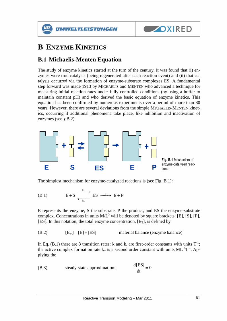
Reactive Transport Modeling – Mar 2011 61
B ENZYME KINETICS
B.1 Michaelis-Menten Equation
The study of enzyme kinetics started at the turn of the century. It was found that (i) en-zymes were true catalysts (being regenerated after each reaction event) and (ii) that ca-talysis occurred via the formation of enzyme-substrate complexes ES. A fundamentalstep forward was made 1913 by MICHAELIS and MENTEN who advanced a technique formeasuring initial reaction rates under fully controlled conditions (by using a buffer tomaintain constant pH) and who derived the basic equation of enzyme kinetics. Thisequation has been confirmed by numerous experiments over a period of more than 80years. However, there are several deviations from the simple MICHAELIS-MENTEN kinet-ics, occurring if additional phenomena take place, like inhibition and inactivation ofenzymes (see § B.2).
Fig. B.1 Mechanism ofenzyme-catalyzed reac-tions
The simplest mechanism for enzyme-catalyzed reactions is (see Fig. B.1):
(B.1) PEESSE k
k
k
E represents the enzyme, S the substrate, P the product, and ES the enzyme-substratecomplex. Concentrations in units M/L3 will be denoted by square brackets: [E], [S], [P],[ES]. In this notation, the total enzyme concentration, [ET], is defined by
(B.2) ]ES[]E[]E[ T material balance (enzyme balance)
In Eq. (B.1) there are 3 transition rates: k and k- are first-order constants with units T-1;the active complex formation rate k+ is a second order constant with units ML-3T-1. Ap-plying the
(B.3) steady-state approximation: 0dt
]ES[d
+ +
E S ES E P

Reactive Transport Modeling – Mar 201162
the rate of product formation can be derived:
(B.4)]S[K
]S[]E[k
dt
]S[d
dt
]P[d
S
T
This is the well known MICHAELIS-MENTEN equation where
(B.5)
k
kkKS (BRIGGS & HALDANE)
Usually, the product of k and [ET] is lumped into a single parameter vmax, which iscalled the maximum rate or maximum reaction velocity:
(B.6) ]E[kv Tmax
KS is known as the half saturation constant measured in concentration units M/L3. Here,‘half’ means if [S] = KS, the formation rate becomes d[P]/dt = ½ vmax.
The MICHAELIS-MENTEN equation contains two parameters: Ks and vmax. There are sev-eral (graphical) approaches to estimate these parameters from batch degradation tests.Limiting conditions for this type of kinetics are listed at the end of this Section.
Equilibrium Approach. Equation (B.4) in combination with Eq. (B.5) was derived firstby BRIGGS and HALDANE in 1925. In the special case of k- >> k, however, Eq. (B.5)simplifies to
(B.7)
k
k
k
kkK kk
S
which was originally formulated by MICHAELIS and MENTEN in 1913. The meaning ofthis assumption is that the formation of the active complex in Eq. (B.1) is much fasterthan the product formation, ES E + P. If this assumption is valid, a pseudo-equi-librium exists between the substrate and the enzyme that can be expressed by the law ofmass action
(B.8)]ES[
]S][E[
k
kKS
(MICHAELIS and MENTEN)
Here KS acts as a dissociation constant of the ES-complex. In this approach, the sub-strate and the enzyme stay in equilibrium with each other while the substrate is beingconsumed. (Note: The equilibrium assumption and the steady-state approximation inEq. (B.3) are quite different things; the first one is more restrictive.)

Reactive Transport Modeling – Mar 2011 63
Order of Kinetics. The MICHAELIS-MENTEN equation (B.4) is plotted in Fig. B.2. Thisequation represents ‘kinetics of mixed order’ (comprising zero- and first-order kinetics).For high substrate concentrations it is of zero order; for small substrate concentration itis of first order:
(B.9) SK]S[ const]E[kdt/]S[d T
(B.10) SK]S[ ]S[dt/]S[d with ST K/]E[k
Fig. B.2 Plot of MICHAELIS-MENTEN
equation
Range of Validity. The application of the MICHAELIS-MENTEN equation requires sev-eral preconditions [Br94]:
1. The reaction must involve a single substrate only (or the concentration of additionalsubstrates must stay constant).
2. Because the reverse reaction (P + S ES) is ignored in Eq. (B.1), initial velocities(= extrapolated values of d[S]/dt at t = 0) must be measured at varying initial sub-strate concentrations [S0].
3. The concentration of the enzyme must be constant.4. [E0] must be much smaller than [S0]; otherwise it is not be possible to apply the
steady-state condition in Eq. (B.3).5. Environmental conditions must be constant (temperature, pH, ionic strength).
B.2 Enzyme Inhibition – HALDANE Equation
Inhibitors are compounds that bind to free enzymes rendering it unusable. Several kindsof inhibitor mechanisms exist. Three major classes of (product) inhibitors are:
competitive inhibition, in which the inhibitor H and substrate S compete for the samereactive site on the enzyme (the alternative substrate H is chemically similar to thesubstrate)
self-inhibition, in which high concentrations of substrate S inhibit the product for-mation. In this case, reaction rates reach a maximum at some intermediate [S] andthen decline as [S] increases. This behavior is described by the so-called HALDANE
formula.
d[P]/dt
[S]KS
vmax
½ vmax

Reactive Transport Modeling – Mar 201164
non-competitive inhibition, in which the inhibitor G and the substrate S may both bebound to the enzyme. The enzyme-substrate-inhibitor complex cannot form prod-ucts.
Self-inhibition (also called substrate inhibition) is a special case of uncompetitive inhibi-tion, in which the inhibitor binds to the enzyme-substrate complex, rather than to thefree enzyme.
Fig. B.3 Three types of inhibitor mechanisms
The three types of inhibitor mechanisms are depicted in Fig. B.3. The corresponding in-hibition-extended MICHAELIS-MENTEN equations are:
(B.11)]S[IK
]S[v
dt
]S[d
1S
max
with
1
1K
]H[1I
(B.12)2S
max
I]S[K
]S[v
dt
]S[d
with
SS
2K
]S[1I
(B.13)3S
max
I
1
]S[K
]S[v
dt
]S[d
with
G
3K
]G[1I
It is quite easy to combine all three inhibition types and incorporate them into a singleexpression:
(B.14)]G[K
K
K/]S[]S[IK
]S[v
dt
]S[d
G
G
SS2
S
max
+
E H EHEH
+
E 2S ESS
+
E S ESG
+
G
]S[IK
]S[v
1S
max
]S[IK
]S[v
1S
max
1
1K
]H[1I
2S
max
I]S[K
]S[v
2S
max
I]S[K
]S[v
2
2K
]S[1I
3S
max
I
1
]S[K
]S[v
3S
max
I
1
]S[K
]S[v
3
3K
]G[1I
competitiveinhibition
self-inhibition(HALDANE)
non-competitiveinhibition

Reactive Transport Modeling – Mar 2011 65
Here the competitive-inhibition term
(B.15)inhjSj K
]j[1I
includes several alternate substrates [j]. The product in Eq. (B.15) runs over all inhibi-tors [j] excluding the ‘self-inhibitor’ S. (In case of reductive degradation dissolved oxy-gen is a non-competitive inhibitor: [G] = [O2], KG = KO2.)
Once again, if there are neither competitive nor non-competitive inhibitors, [j] = 0 and[G] = 0, Eq. (B.14) reduces to the HALDANE equation:
(B.16)SS
2S
max
K/]S[]S[K
]S[v
dt
]S[d
(HALDANE equation)
which is equivalent to Eq. (B.12). Here, KSS is the HALDANE parameter.
Allosteric Inhibition. So far, only conventional inhibitors were considered which affectenzyme activity by direct interaction with the active site. By contrast, allosteric inhibi-tors modify enzyme activity by binding at sites remote from the catalytic site, thus caus-ing conformational changes (enzymes become inactive). Allosteric inhibition is not con-sidered in the model.
B.3 Microbial Growth Dynamics – MONOD Kinetics
Microorganisms, mainly bacteria, occur ubiquitously in the subsurface. In groundwaterthey usually form colonies attached as biofilms on the matrix of porous media or frac-tured surfaces.
In this Section we establish a link between enzyme kinetics and microbial growth dy-namics (population dynamics). At first glance, the expressions of enzyme kinetics andof microbial growth seem to be quite the same. But this is not strictly true. In contrast,we have to deal with two completely different concepts developed at different times andwithout any reference to each other (see Tab. B.1).
The heart of MONOD’s theory is the concept relating microbial growth rate, , with lim-iting substrate concentration, [S]. The empirical formula MONOD derived in 1942 was
(B.17)]S[K
]S[
S
max
(MONOD equation)
with max as the maximum rate in units of inverse time, T-1. It is interesting to note, thatoriginally MONOD did not draw any parallel between his equation and the MICHAELIS-MENTEN equation. The microbial growth rate determines the population dynamics, i.e.the change in biomass or cell density
(B.18) B)(dt
dB

Reactive Transport Modeling – Mar 201166
where B is the biomass or cell density and denotes the cell death rate [T-1]. Eq. (B.18)is a first-order rate equation. Due to the same mathematical form as in the MICHAELIS-MENTEN equation (hyperbolic form) the MONOD equation implies that approachesasymptotically the value max that remains constant while [S] increases (similar to thecurve in Fig. B.2 at page 63).
Tab. B.1 Enzyme kinetics vs. population dynamics (basic concepts)
It is a matter of fact that the (total) number of enzymes, ET, and the biomass B are corre-lated: The greater the biomass the more enzymes are present to degrade the substrate. Ina good approximation, enzyme and biomass concentrations should be proportional,[ET] B. Both quantities are tied together by the so-called yield coefficient Y (a kind of‘generalized stoichiometric coefficient’):
(B.19) BY
]E[k maxT
Using the formulas in Tab. B.1, the dynamics of an ‘unisubstrate model’ is described bythe following set of differential equations:
(B.20) )t(BY
)t(
dt
]S[d
(B.21) )t(B)t(dt
dB
(B.22)]S[K
]S[)t(
S
max
enzyme kinetics population dynamics
MICHAELIS, MENTEN 1913 MONOD 1942
dynamical variable: substrate [S] biomass or cell density B
]S[K
]S[v
dt
]S[d
S
max
]E[kv Tmax
]S[K
]S[
S
max
B)(dt
dB
deduced from well-defined assumptionsabout the catalytic mechanism
empirical equation