Reading expRess Lesson sampLeR Level H (Grade 8), Lesson

Annales Geophysicae (2004) 22: 3869–3887SRef-ID: 1432-0576/ag/2004-22-3869© European Geosciences Union 2004

AnnalesGeophysicae

Turbulent diffusivity in the free atmosphere inferred from MSTradar measurements: a review

R. Wilson

Service d’Aeronomie/IPSL, Universite P. et M. Curie, Paris, France

Received: 15 December 2003 – Revised: 16 June 2004 – Accepted: 24 June 2004 – Published: 29 November 2004

Part of Special Issue “10th International Workshop on Technical and Scientific Aspects of MST Radar (MST10)”

Abstract. The actual impact on vertical transport of small-scale turbulence in the free atmosphere is still a debated is-sue. Numerous estimates of an eddy diffusivity exist, clearlyshowing a lack of consensus. MST radars were, and con-tinue to be, very useful for studying atmospheric turbulence,as radar measurements allow one to estimate the dissipationrates of energy (kinetic and potential) associated with turbu-lent events. The two commonly used methods for estimatingthe dissipation rates, from the backscattered power and fromthe Doppler width, are discussed. The inference methods ofa local diffusivity (local meaning here “within” the turbulentpatch) by using the dissipation rates are reviewed, with someof the uncertainty causes being stressed. Climatological re-sults of turbulence diffusivity inferred from radar measure-ments are reviewed and compared.

As revealed by high resolution MST radar measurements,atmospheric turbulence is intermittent in space and time. Re-cent theoretical works suggest that the effective diffusivity ofsuch a patchy turbulence is related to statistical parametersdescribing the morphology of turbulent events: filling factor,lifetime and height of the patches. It thus appears that a sta-tistical description of the turbulent patches’ characteristicsis required in order to evaluate and parameterize the actualimpact of small-scale turbulence on transport of energy andmaterials. Clearly, MST radars could be an essential tool inthat matter.

Key words. Meteorology and atmospheric dynamics (turbu-lence; instruments and technique) – Radio science (remotesensing)

1 Introduction

Small-scale turbulence is a very essential process of atmo-spheric and oceanic dynamic since (i) it is the sink for me-chanical energy through dissipative processes, (ii) it induces

Correspondence to:R. Wilson([email protected])

drag on the large-scale flow through Reynolds stress, (iii) itinduces irreversible transport of heat, mass and minor con-stituents. However, the actual impact of small-scale turbu-lence on the atmospheric dynamic – energy budget and ver-tical transport – is still an open issue. For instance, the ques-tion as to whether the small-scale turbulence has any signif-icant impact on vertical transport in the upper-tropospherelower-stratosphere (UTLS), and in the mesosphere as well,is still debated.

Various evaluations of the turbulent diffusivityKθ (m2/s)for the UTLS and for the mesosphere are shown in Table1.In this table are reported estimations of the diffusivity in-ferred either from indirect methods – by combining the ob-servations of tracer profiles and a mathematical model fortransport, production and losses – or from direct measure-ments of energetics parameters of turbulence, are reported.These estimations can hardly be directly compared however,as they have sometimes very different meanings.

Some of these evaluations are bulk transport coefficients,i.e. on a planetary scale. The vertical transport terms areevaluated by taking into account the production and loss pro-cesses on large space and time scales (several weeks) (Massieand Hunten, 1981; Ogawa and Shimazaki, 1975). However,the actual impact of small-scale turbulence cannot be di-rectly retrieved from these values, as other non-turbulent pro-cesses might contribute to vertical transport as the (diabatic)Brewer-Dobson circulation.

A small impact on vertical transport in the lower strato-sphere (Kθ∼0.01−0.02 m2/s or less) was inferred from thein-situ observations of filamentary structures of tracers andby using a numerical model representing the stretching andmixing processes (Waugh, 1997; Balluch and Haynes, 1997).On the other hand,Legras et al.(2003), by combining ob-served ozone profiles and a stochastic-dynamical model forreconstructing the profiles, found a much more significantimpact (Kθ≈0.1 m2/s or larger).

Further difficulties arise when comparing the diffusiv-ity estimates inferred from measurements. Some evalua-tions are local ones (i.e. within the turbulent patches), either

3870 R. Wilson: Turbulent diffusivity from MST radar measurements: a review

Table 1. Various estimations of atmospheric diffusivity (m2/s) for the UTLS and mesosphere.

Various estimates forKθ (m2/s)

Indirect In-situ Radar

Free Troposphere ∼10 (Massie and Hunten, 1981) 0.02−0.8 0.3−3(Alisse and Sidi, 2000a) (Nastrom and Eaton, 1997)

2–111 [mean 42] 0.3−3 (Rao et al., 2001)(Kennedy and Shapiro, 1980)

0.2−2 (Kurosaki et al., 1996)

Lower Stratosphere 0.2−0.6 0.46−1.2 [eff. 0.01−0.06] 0.1−0.5 (Fukao et al., 1994)(Massie and Hunten, 1981) (Lilly et al., 1974)

∼ 0.01−0.02 (Waugh, 1997) 0.1−0.35 0.5−1(Balluch and Haynes, 1997) (Alisse and Sidi, 2000a) (Nastrom and Eaton, 1997)

∼0.1 (Legras et al., 2003) 0.01−0.1 (Bertin et al., 1997) 0.05−0.3 (Rao et al., 2001)

0.2−0.3(Woodman and Rastogi, 1984)

Mesosphere 20−200 3.5−70 (Lubken, 1992) 1−30 (Fukao et al., 1994)(Ogawa and Shimazaki, 1975) (Lubken et al., 1993) (Kurosaki et al., 1996)

3−10 (Rao et al., 2001)

100−200 (Hocking, 1988)

20−150 (Roper, 2000)

from in-situ measurements (e.g.Lilly et al., 1974; Barat andBertin, 1984; Lubken, 1992; Alisse and Sidi, 2000a), or fromradar measurements (e.g.Hocking, 1988; Fukao et al., 1994;Roper, 2000; Rao et al., 2001). Other estimates are inferredfrom an evaluation of the heat (or tracer) flux across a givenheight level, by using both local evaluations of turbulencestrength and fractional time of turbulent events. These evalu-ations thus take into account, in some aspects, the space-timeintermittency of turbulence (e.g.Lilly et al., 1974; Woodmanand Rastogi, 1984) (the values between brackets are fromLilly et al. (1974) in the table). Furthermore, some estimatesare Eulerian, as radar measurements (a fixed volume beingsampled), others being performed quasi-instantaneously, ei-ther at a quasi-constant height level (instrumented aircrafts)or along a quasi-vertical profile (balloons or rockets borneinstruments).

In fact, there exists a certain confusion in the literaturewhen comparing these “turbulent diffusivities”. One can,however, observe at this stage that, beyond the natural vari-ability of turbulence strength, the dispersion of these “effec-tive” diffusivity estimates (two to three orders of magnitude)reveals a lack of consensus about the actual impact of small-scale turbulence on transport processes (Table1).

MST radars have the unique ability to allow for measure-ments related to the energetics of small-scale turbulence witha high space-time resolution, in the UTLS and in the meso-sphere. The aim of this paper is to review and discuss the

methods used in evaluating the turbulence diffusivity fromMST radar measurements. In Sect.2, the main character-istics of turbulence in the free atmosphere are described:length scales, energetics and related diffusivity. The infer-ence of turbulent diffusivity from radar measurements is atwo-step process. First, the turbulence strength is character-ized, usually from the KE dissipation rate,εk. Second, theturbulent diffusivity is evaluated by assuming a relationshipbetween the dissipation rateεk and the heat flux (or buoy-ancy flux). The two commonly used methods for estimatingεk, from the structure constantC2

n or from the turbulent ve-locity varianceu2, are described in Sect.3. We also introducethe equations describing the (unfamiliar) turbulent potentialenergy (balance equation, dissipation rate) and its relationto mixing. Indeed, as noticed byHocking and Mu(1997);Hocking (1999), the structure constantC2

n is a quantity re-lated to the potential energy of the turbulent flow. On theother hand, numerous authors showed that mixing events ina stratified flow lead to a change in the background poten-tial energy through the dissipation of available potential en-ergy (Dillon and Park, 1987; McIntyre, 1989; Winters et al.,1995). The estimation of a turbulent diffusivity from radarmeasurements relies on measured quantities (εk or C2

n) butalso on non-measured parameters (i.e. local stratification,mixing efficiency, filling factor). that have to be evaluatedindependently. This point will be discussed in some detail inSect.4. Quantitative results are described in the following

R. Wilson: Turbulent diffusivity from MST radar measurements: a review 3871

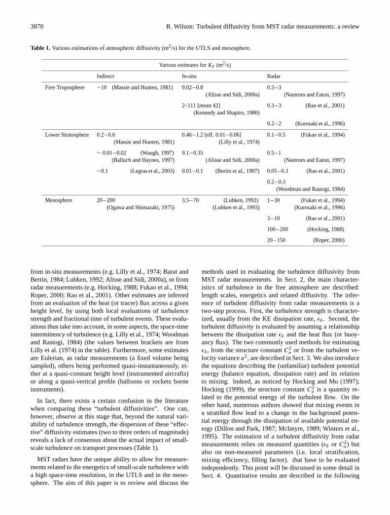
Fig. 1. Power spectrum of relative density fluctuations together with Tatarskii’s (1971) theoretical model (fromLubken, 1992).

section. Climatological studies of turbulence diffusivity in-ferred from radar measurements are reviewed and discussed.Comparative studies of radar methods are also reviewed.

A key issue in evaluating the actual diffusive properties ofsmall-scale turbulence in the atmosphere (and ocean as well)is the intermittency. In the last part of the paper, theoreti-cal and semi-empirical works on the diffusive properties ofa patchy turbulence are presented. A few suggestions for fu-ture radar studies will also be advanced.

2 Inertial turbulence in a stratified atmosphere

Turbulent motions in a stratified medium induce fluctuationsof velocity but also of tracers, such as temperature, humidity,or refractive index. Numerous evidences of an inertial sub-range “a la Kolmogorov” were observed “in-situ” in the freeatmosphere from micro-structures measurements (e.g.Barat,1984; Barat and Bertin, 1984; Sidi and Dalaudier, 1990;Lubken, 1992). The inertial turbulent subrange is character-ized by a−5/3 spectral index for 1-D (observable) spectraof the velocity or tracers’ fluctuations (Fig.1, from Lubken,1992).

It is important to note that the energy spectrum of air mo-tions is also characterized by ak−5/3-range (k being the hori-zontal wave number) in the mesoscale region, i.e. from wave-lengths of some few km to wavelengths of about 500 km

(Gage, 1979; Nastrom and Gage, 1985). There is still adebate about the interpretation of such a spectrum.De-wan(1979) andVanZandt(1982) explained thek−5/3-rangeby a direct energy cascade of gravity waves (from large tosmall scales). On the other hand,Gage(1979) interpretedthek−5/3-spectrum as the spectrum of 2-D turbulence with anegative energy flux (from small to large scales). In a recentpaper, by considering the second and third order structurefunctions,Lindborg (1999) brought support to the first hy-pothesis (i.e. the wave hypothesis), at least for thek5/3 range.In any event, such ak−5/3-spectrum must not be interpretedas the spectrum of inertial turbulence, and cannot be usedin order to infer small-scale turbulence parameters (TKE ordissipation rates).

2.1 Turbulent scales

A variety of turbulence scales were defined. Two importantlength scales are the outer scaleLm, characterizing the sizeof the largest turbulent eddies of the inertial range, and theinner scalelo, a transition scale between the inertial and theviscous ranges. The outer scale (sometimes labelled the in-tegral scale) is related to the rms wind velocityu and TKEdissipation rateεk in the inertial range through (e.g.Tennekesand Lumley, 1972, p 20):

Lm ∼ u3/εk . (1)


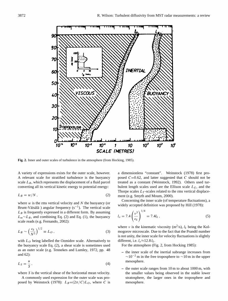
Fig. 2. Inner and outer scales of turbulence in the atmosphere (fromHocking, 1985).

A variety of expressions exists for the outer scale, however.A relevant scale for stratified turbulence is the buoyancyscaleLB , which represents the displacement of a fluid parcelconverting all its vertical kinetic energy to potential energy:

LB = w/N , (2)

wherew is the rms vertical velocity andN the buoyancy (orBrunt-Vaisala ) angular frequency (s−1). The vertical scaleLB is frequently expressed in a different form. By assumingLm∼LB , and combining Eq. (2) and Eq. (1), the buoyancyscale reads (e.g.Fernando, 2002):

LB ∼

( εk

N3

)1/2≡ LO , (3)

with LO being labelled the Ozmidov scale. Alternatively tothe buoyancy scale Eq. (2), a shear scale is sometimes usedas an outer scale (e.g.Tennekes and Lumley, 1972, pp. 48and 62):

LS =u

S, (4)

whereS is the vertical shear of the horizontal mean velocity.A commonly used expression for the outer scale was pro-

posed byWeinstock(1978): LB=(2π/C)LO , whereC is

a dimensionless “constant”.Weinstock (1978) first pro-posedC=0.62, and latter suggested thatC should not betreated as a constant (Weinstock, 1992). Others used tur-bulent length scales used are the Ellison scaleLE , and theThorpe scalesLT -scales related to the rms vertical displace-ment (e.g.Smyth and Moum, 2000).

Concerning the inner scale (of temperature fluctuations), awidely accepted definition was proposed byHill (1978):

lo = 7.4

(ν3

εk

)1/4

= 7.4lk , (5)

whereν is the kinematic viscosity (m2/s), lk being the Kol-mogorov microscale. Due to the fact that the Prandtl numberis not unity, the inner scale for velocity fluctuations is slightlydifferent, i.e.lo≈12.8 lk.

For the atmosphere (Fig.2, from Hocking1985):

– the inner scale of the inertial subrange increases from∼10−2 m in the free troposphere to∼10 m in the uppermesosphere.

– the outer scale ranges from 10 m to about 1000 m, withthe smaller values being observed in the stable lowerstratosphere, the larger ones in the troposphere andmesosphere.


Evaluations of inner and outer scales in the UTLS (5–20 km)are reported inEaton and Nastrom(1998). These scales areinferred from radar estimates of the TKE and related dissipa-tion rate. Inner scale values were observed to increase from1 cm at 5 km to about 8 cm at 20 km altitude. The outer scale(shear scale) is found to range from∼10 m (lower strato-sphere) to∼65 m (free troposphere). By combining rocketand radar data,Watkins et al.(1988) observed an inner scaleranging from 2 to 6 m in the upper mesosphere (80 to 90 kmheight domain).

2.2 Energetics

Typically, energy (kinetic or potential) of turbulent motionsranges from∼10−2 J/kg in the lower stratosphere to about1–10 J/kg or so in the free troposphere and mesosphere(Fukao et al., 1994; Nastrom and Eaton, 1997; Alisse andSidi, 2000a; Lubken, 1992; Hall et al., 1999). By noting thatεk∼u3/Lm (Eq.1) and assumingLm∼LB leads to:

εk ∼ u2N . (6)

The dissipation rate is thus∼10−2×TKE, typically.

The turbulence intensity is usually characterized from theTKE per unit mass (J/Kg)

EK =1

2(u2

+ v2+ w2) , (7)

whereu, v, w are the rms turbulent velocities. One importantcharacteristic of stratified turbulence is that a fraction of TKEis converted into available turbulent potential energy (TPE)

EP =1

2N2ζ 2

=1

2

g2

N2

θ2

θ2

, (8)

whereθ is the generalized potential temperature (Ottersten,1969b), θ being a reference state,ζ is the rms vertical dis-placement inferred from the potential temperature variance(i.e. the Ellison scale). It is precisely that fraction of energywhich is related to the heat (and mass) transport. Indeed,Eq. (8) shows that the dissipation of temperature variance in-duces a dissipation of TPE (later discussed). In a stratifiedmedium (dθ/dz>0), the dissipation of (potential) tempera-ture variance, in reducing the stratification, induces a down-ward heat flux.

The equation describing the time evolution of TKE in astratified medium reads (Tennekes and Lumley, 1992, p. 63;Gill, 1982, pp. 76–78)

dEK

dt= P − B − εk + ∇ · FK , (9)

where∇·FK is a transport term through surface fluxes,P

is the production term through Reynolds stress acting in ashear, andB is the buoyancy flux, expressing a reversibleconversion of TKE into TPE,

P = −u′w′du

dz; B = −

g

θw′θ ′ . (10)

The time evolution of temperature variance reads, (Ten-nekes and Lumley, 1972, p. 95)

1

2

dθ ′2

dt= −w′θ ′

dθ

dz− εθ + ∇ · Fθ , (11)

where εθ is the dissipation rate of half temperature vari-ance,with∇·Fθ being a transport term. By noting that thetemperature variance is related to the TPE (Eq.8), one ob-tains an equation for the time evolution of TPE by multiply-ing Eq. (11) by (g/Nθ)2:

dEP

dt= B − εp + ∇ · Fp . (12)

The buoyancy flux is here a source term for TPE, dissipatedthrough thermal diffusivity (εp ∝ εθ ). Therefore, the dissipa-tion rate of temperature variance,εθ , can be interpreted as adissipation rate of available potential energy.

Two simplifying assumptions are typically made (likelydue to the lack of alternative possibilities). By assuming spa-tial homogeneity, the divergence terms vanishes. By furtherassuming stationarity, the balance equations for TKE andTPE reduce to

P − B = εk (13)

B = εp . (14)

The productionP of TKE is balanced by the buoyancy fluxB(reversible conversion into TPE) and the dissipationεk (irre-versible). The production term of TPEB is simply balancedby the dissipation rateεp.

2.3 Turbulent diffusivity

The diffusive properties of turbulence are commonly ex-pressed from the heat flux8θ=ρCpw′θ ′ (ρ is atmo-spheric density,Cp the specific heat at constant pres-sure). The eddy diffusion coefficient for heat is defined asKθ=−w′θ ′/(dθ/dz).

From Eq. (14) an indirect evaluation of the diffusivity canbe estimated from the dissipation rate of temperature vari-ance (Osborn and Cox, 1972)

Kθ =εθ

(dθ/dz)2. (15)

Equivalently, with the above notations, (multiplying the nu-merator and denominator of Eq. (15) by (g/Nθ)2) one ob-tains:

Kθ =εp

N2. (16)

Another indirect evaluation, from the TKE dissipation rate,is inferred from Eq. (13) (Lilly et al., 1974; Osborn, 1980):

Kθ = γεk

N2, (17)

whereγ is sometimes referred to as the mixing efficiency.Under the above hypotheses of homogeneity and stationarity,γ reads

γ =B

P − B=

Rf

1 − Rf

=εp

εk

, (18)


whereRf =B/P is the flux Richardson number. As noticedby several authors however, the efficiency of mixing shouldrather be defined as the fraction of the supplied energy thatis actually used for mixing, that isB/P=Rf , rather thanγ .We therefore chose to simply labelγ as the dissipation ratesratio.

3 Radar measurements of the turbulence energetics

Radar measurements related to small-scale turbulence areusually the reflectivity and the wind velocity variance. Un-der the hypothesis that the inhomogeneities of refractive in-dex are due to homogeneous and stationary inertial turbu-lence, the reflectivity is a simple function of the structureconstantC2

n Tatarskii(1961); Ottersten(1969a). C2n can be

interpreted as the mean squared-difference of refractive in-dex for unity distance (i.e. the value of the structure functionfor one meter separation). The wind velocity variance relatesto the TKE, provided that the non-turbulent contributions tothat variance can be removed. A variety of radar techniquesexist for estimating the wind velocity: from the line-of-sightvelocity differences from meteors (Roper, 1966); from theimaging Doppler interferometry scattering positions (Roperand Brosnahan, 1997), from spaced antenna full correla-tion analysis (Briggs, 1980; Manson et al., 1981), and fromthe spectral broadening observed by MST Doppler radars.(Hocking, 1983). This last technique, applicable for nar-row beams VHF and UHF radars, was widely used fromthe troposphere to the mesosphere. The other techniques,mostly based on MF radars measurements, were rather usedin studying the mesospheric dynamics. A comparative dis-cussion about these techniques is beyond the scope of thispaper. However, some of the approximations and assump-tions of the inference methods of turbulence parameters areindependent of the measurement techniques.

In the following of this section, we shall mostly discussthe two commonly used measurement methods for turbu-lence studies from MST radars. Following the terminologyof Cohn(1995), the method relying on the reflectivityη, orrelatedC2

n, to the dissipation rateεk, will be labelled the“power method”. The method relying on the Doppler widthto εk, will be also labelled the “spectral width method”. Newradar methods for estimating the dissipation rateεk will alsobe briefly mentioned. Again, the subject of this paper is notto review radar techniques used for turbulence measurements(some good articles exist, e.g.Hocking, 1985, 1997; Cohn,1995; Hocking and Mu, 1997) but rather to discuss the meth-ods used to infer the turbulent diffusivity from radar mea-surements of reflectivity and wind velocity variance.

3.1 The power method

The power method relates the radar reflectivity to the struc-ture constant of refractive indexC2

n (VanZandt et al., 1978;Gage et al., 1980), by assuming that the reflecting layersare due to inertial and (locally) homogeneous turbulence.

In other words, the basic assumption of this method is thatthe scattering process is Bragg scattering due to isotropic re-fractive index inhomogeneities (Tatarskii, 1961). Support-ing this hypothesis, a direct comparison between high reso-lution in-situ measurements of refractive index fluctuationsand oblique radar backscattered power was successfully con-ducted byLuce et al.(1996). Of course, the power methodrequires a radar calibration. The power method can onlybe applied if other sources of (back)scattering can be ne-glected. Non-turbulent causes of radio waves scattering in-clude Rayleigh scattering (from hydro-meteors or insects, in-volving UHF radars) and Fresnel scattering (partial reflec-tion, involving VHF radars). By comparing high-resolutionin-situ measurements and vertical power of a VHF radar,Luce et al.(1995) showed that partial reflection from tem-perature sheets, described byDalaudier et al.(1994), is likelyto be the main mechanism contributing to vertical echo en-hancements.

The isotropic scatterers (i.e. isotropic refractive index in-homogeneities) are thought to be the dominant scatteringprocess for zenith angles larger than∼10–15◦(e.g. Tsudaet al., 1986; Hocking et al., 1990), although aspect sensitiv-ity was observed in some cases for zenithal angles as largeas 20◦(Tsuda et al., 1997a), and even 30◦(Worthington et al.,1999a,b). Aspect sensitivity has not been observed for UHFradars. Several authors also reported radar observations of anazimuthal anisotropy of the backscattered power of obliquebeams (e.g.Tsuda et al., 1986; Hocking et al., 1990; Hooperand Thomas, 1995; Worthington and Thomas, 1997; Wor-thington et al., 1999b). Such an anisotropy of backscat-tered power is believed to be due to the tilting of aspectsensitive surfaces by gravity waves and vertical wind shears(Worthington and Thomas, 1997), i.e. it is not a turbulenceinduced effect. However, another hypothesis for the VHFzenithal aspect sensitivity relies on the turbulence anisotropy(e.g.Tsuda et al., 1997a). For a review on the aspect sen-sitivity of VHF radar echoes, seeLuce et al.(2002b). Inany event, such aspect sensitive scatterers may induce er-ror (over-estimation) in evaluating the isotropic-turbulenceintensity.

Within a stratified medium, the refractive index fluctua-tions δn are induced by vertical displacementδz (Tatarskii,1961)

δn = Mδz , (19)

whereM is the gradient of generalized potential index forunionized atmosphere (Tatarskii, 1961; Ottersten, 1969b):

M=−0.776×10−6P

T

[(1+15 500

q

T

)N2

g−

15 500

2T

∂q

∂z

],(20)

whereP is the pressure (Pa),T the temperature (K),q thespecific humidity (g/g). If humidity can be neglected, as it isthe case in the stratosphere,M depends on the static stabilityonly:

M = −0.776× 10−6P

T

N2

g. (21)


Note that, in the mesosphere,M also depends on the electrondensity.

Vertical displacements inducing a conversion into (avail-

able) TPE (Eq.8), and noting that(δz2)1/2

≈ζ , one can ex-

pressEP as a function of the variance of refractive indexfluctuationsδn2:

EP =1

2N2ζ 2

=1

2

(N

M

)2

δn2 . (22)

The dissipation of refractive index variance (εn) can thus beexpressed as a function of the dissipation rate of TPE (εp).From Eq. (22):

εp =

(N

M

)2

εn . (23)

Under the assumption of isotropic inertial turbulence, the 3Dspectrum of refractive index fluctuations is proportional tothe structure constantC2

n (Tatarskii, 1961, pp. 46–58), thatis:

C2n = a2 εn

ε1/3k

. (24)

As a function of the TPE dissipation rate Eq. (23), the struc-ture function reads:

C2n = a2

(M

N

)2 εp

ε1/3k

. (25)

Hence, the structure constantC2n is related to both the dissi-

pation rates of TPE and TKE. One can therefore expressC2n

either as a function ofεk (e.g.VanZandt et al., 1978; Hock-ing, 1999):

C2n = γ a2

(M

N

)2

ε2/3k (26)

or as a function ofεp (Dole et al., 2001)

C2n = γ 1/3a2

(M

N

)2

ε2/3p . (27)

As noticed by numerous authors (e.g.VanZandt et al.,1978; Gage et al., 1980), a further complication comes fromthe fact that the radar reflectivityη, and thus the inferredC2

n, are weighted volume averages (<η>vol and<C2n>vol)

(a uniform reflectivity within the sampling radar volume isassumed):

< C2n >vol= FT C2

n , (28)

whereFT is the turbulent fraction of the sampled volume.Therefore, the local dissipation rates (within the turbulentlayer) must be expressed as a function of the volume aver-aged<C2

n>vol ;

εk =1

γ 3/2

(1

a2

N2

M2

< C2n >vol

FT

)3/2

(29)

εp =1

γ 1/2

(1

a2

N2

M2

< C2n >vol

FT

)3/2

. (30)

The inferred dissipation rates only differ by the power of theγ term. Theεp estimate is rather more robust, showing aweaker dependency on the unknownγ term, than theεk es-timate (Dole and Wilson, 2000). Indeed, the refractive indexfluctuations are rather related to potential energy (dependingon vertical motions and stratification) than to kinetic energy.Notice, however that these two expressions for the dissipa-tion rates (Eqs.29 and 30) lead to an equivalent turbulentdiffusivity Kθ (Eqs.16and17).

3.2 The spectral width method

Turbulent motions induce a widening of the velocity distribu-tion and thus a spectral broadening of the backscattered echo.But other non-turbulent processes also contribute to the spec-tral broadening (e.g.Hocking, 1985; Gossard and Strauch,1983; Nastrom and Eaton, 1997):

– beam and shear broadening, related to the beam geo-metry;

– wave or 2-D turbulence contamination.

The non-turbulent effects must be removed. With the variouscauses of broadening being independent of each other, theinduced variances simply add, i.e.:

σ 2obs = σ 2

T + σ 2B+S + σ 2

W , (31)

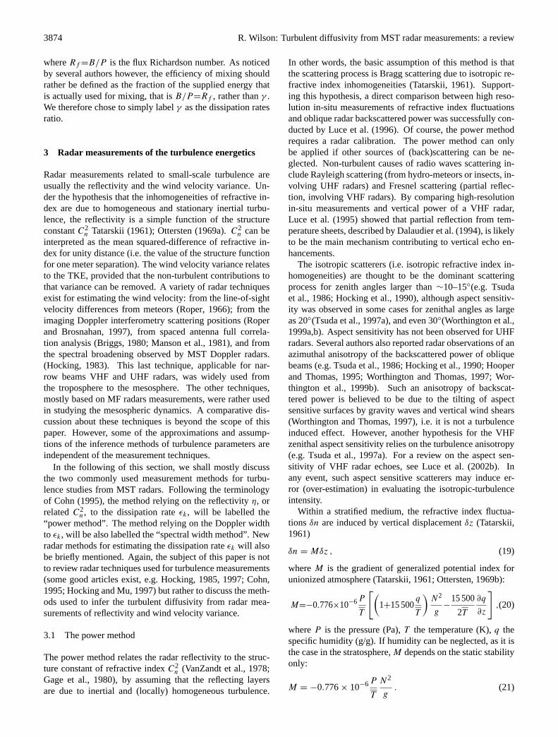
whereσobs is the observed spectral width (half power-halfwidth in Hz), σT being the turbulent contribution to thatbroadening. Beam and shear broadeningσB+S have to beevaluated from the known wind velocity profile, taking intoaccount the beam geometry.Nastrom and Eaton(1997), Chu(2002), andVanZandt et al.(2002) presented formulae thataccounts for the background wind speed across a radar beam.The wave (or 2-D turbulence)σW can be reduced a by shortintegration time (e.g.Cohn, 1995), or by using a wave model(Hocking, 1988; Nastrom and Eaton, 1997).

The rms turbulent velocity relates toσT asu=(λr/2)σT /

√(2 ln 2). Nastrom and Eaton(1997) ob-

served that, for the narrow beam WSMR radar (2.9◦oneway 3 dB beamwidth), the beam broadening is generallythe largest correction term by far (WSMR stands for WhiteSand Missile Range). Figure3, from Nastrom and Eaton(1997), shows mean profiles of the observed spectral width,compared to the applied corrections (total correction and thedifferent terms).

A new radar technique for removing these non-turbulent(deterministic) effects has been recently proposed byVanZandt et al.(2002). The basic idea is to evaluate thebroadening with two different beamwidths, the correctionterms being approximately proportional to the beamwidthsquared. The two beamwidth method has the advantageof being less sensitive than the standard single-beamwidth


Fig. 3. Mean vertical profiles of the observed width with the correc-tions due to beam broadening, shear broadening and gravity-waveeffects fromNastrom and Eaton(1997).

method to the necessary instrumental corrections of the ob-served spectral widthσobs .

Nastrom and Tsuda(2001) observed significant differ-ences between the spectral widths from beams in two orthog-onal planes – zonal and meridional – at both the MU (Middleand Upper atmosphere) radar and the WSMR radar. Such ananisotropy may be an effect due to the horizontal wind direc-tion relative to the antenna beams (Chu, 2002).

The spectral width method has several advantages over thepower method. First, there is no need for an absolute calibra-tion of the radar. Second, the radar estimate of the velocityvariance is a reflectivity and range weighted average (Doviakand Zrnic, 1993, pp. 109–110), i.e. the non-turbulent (non-reflecting) regions of the sampled volume do not contribute.The variance estimate is thus a weighted average on turbulentpatches only. On the other hand, the turbulent velocity vari-ance is related to the TKE dissipation rate. Consequently,there is no need for further information about the turbulentfraction or the dissipation ratioγ , in order to retrieveεk. Ifconcerned with mixing, however, (i.e. vertical transport ofheat or mass) the turbulent diffusivity is only indirectly re-lated to the TKE dissipation rate (through the energy conver-sion rateB or the dissipation rates ratioγ ).

Two methods were proposed (discussed byHocking,1999) in order to relate the measuredu2 to εk.

– If the radar volume is filled with homogeneous turbu-lence, the observed variance results from the convolu-tion of the velocity fluctuation field with the weightedsampling volume. By assuming a Kolmogorov spec-trum, as well as a Gaussian shaped sampling volume,the dissipation rate reads (Frisch and Clifford, 1974;Gossard and Strauch, 1983):

εk =1

δ

[u2

1.35α[1 − β2/15]

]3/2

, (32)

where

{δ = σb ; β2

≈ 1 − (σr/σb)2 if σr < σb

δ = σr ; β2≈ 4(1 − (σb/σr)

2) if σb < σr.

– If the outer scale of turbulence is smaller than any scaleof the sampled volume, the relationship between thevariance (i.e. TKE) and the dissipation rate is ratherdependent on the outer scaleLm (Sato and Woodman,1982; Hocking, 1983). Weinstock(1978) suggested thatthis outer scale is likely proportional to the OzmidovscaleLO

Lm ≈ 3πLO ∼ 3π( ε

N3

)1/2. (33)

Therefore

εk ≈ 0.47u2 N . (34)

This last relationship is widely used in most MST radarsstudies of atmospheric turbulence. Notice, however, that therelation betweenLm andLO (Eq. 33) has been questionedby Weinstock(1992), as it seems to lead to too high a valuefor the dissipation rates ratio.

A variant of the spectral width method, sometimes labelledas the “variance method”, is based on the direct estimation ofthe wind velocity variance from the velocity spectrum (e.g.Hall et al., 2000; Satheesan and Murthy, 2002). These au-thors assumed that motions are turbulent for short time fluc-tuations, in order to estimateεk from Eq. (34). However,some caution must be taken in this case as a−5/3 spectralindex is not undoubtedly the signature of inertial turbulence.Satheesan and Murthy(2002) presented a comparative studyof methods for retrieving the dissipation rateεk (to be dis-cussed later).

3.3 Direct estimation ofεk: the two-wavelengths method

A new radar technique was recently proposed byVanZandtet al.(2000), allowing for a direct estimations of the TKE dis-sipation rate. These authors used the ratio of simultaneousobservations of radar reflectivity for two wavelengths closeto the viscous scale, together with Hill’s model of refractivityfluctuations due to turbulence (Hill , 1978; Frehlich, 1992).When neglecting scattering from particulates, the radar re-flectivity η(λ) (m2/m2) reads

η(λ) = 0.38C2

n

λ1/3H(λ, εk) , (35)

where theH(λ, εk) term takes into account the departurefrom the standard Kolmogorov model for the temperaturefluctuations for scales close to the dissipation scale. Withthis dual-wavelengths technique most non-turbulent echoesare identified and filtered out.

4 Stratification and unknown parameters

Detailed knowledge of the local atmospheric conditions isneeded for the correct interpretation of radar observations


(Eqs.29 or 34 for instance). Furthermore, the relationshipsbetween diffusion and energy dissipation rates rely on strat-ification (Eqs.16 and17). Depending on the method used,several additional parameters have to be evaluated: buoyancyfrequencyN and gradient of generalized refractive indexM,turbulent fractionFT , as well as the dissipation rates ratioγ .Various methods or strategies have been proposed.

4.1 Local atmospheric conditions

The local stratification (within the radar sample volume) isdescribed byN andM. Both parameters are needed for re-lating C2

n to the dissipation rates (power method, Eqs.29and 30). The buoyancy frequency is also used in relatingthe TKE toεk (spectral width method, Eq.34). Furthermore,the turbulent diffusivityKθ is related to the dissipation ratesthroughN2 (Eqs.16and17).

In the upper troposphere and lower stratosphere the spe-cific humidity is negligible;M depends mainly on the buoy-ancy frequencyN . In most cases, the localN is evaluatedfrom additional in-situ measurements – usually from stan-dard meteorological soundings. However, as observed byDalaudier et al.(2001), the use of in-situ soundings doesnot allow for valuable estimations of the local stratification(within the radar volume) – at least for vertical resolutionsof ∼150 m – likely because of the large variability ofN onrelatively small time-and-space scales. The most probableexplanation for such a rapid time and space evolution of thestability profile is the propagation of gravity waves. A goodestimator – in the sense of the mathematical expectation ofa random variable – remains likely the bulk buoyancy fre-quency, obtained either from a model (climatological or nu-merical), or from standard meteorological soundings with alow vertical resolution.

In the troposphereM depends on both the Brunt-Vaisalafrequency and humidity gradientdq/dz (Eq. 20). In thiscase, the humidity gradient must necessarily be estimatedfrom additional measurements. New data processing meth-ods for retrieving the humidity profile by combining theradar reflectivity with additional measurements were recentlyproposed: with RASS (Radio Acoustic Sounding System)(Tsuda et al., 2001), GPS (Global Positioning System) (Gos-sard et al., 1998), or balloon-borne instruments (Mohan et al.,2001; Wilson and Dalaudier, 2003). Clearly, such combina-tions of instruments are very promising for future turbulencestudies.

4.2 The turbulent fraction

The turbulent fraction,FT , must be evaluated in order to re-trieve the localC2

n from the volume-averaged<C2n>vol . On

the other hand, as will be further discussed in Sect.6, a statis-tical description of turbulent events (layers depths, lifetime,filling factor, intensity) is required for estimating the effec-tive diffusivity of a patchy turbulence (Hocking and Rottger,2001).

In-situ measurements – from instrumented aircrafts – inthe lower stratosphere suggest 0.02<FT <0.05 (Lilly et al.,1974). From six balloon soundings of temperature and windmicrostructures,Alisse and Sidi(2000a) observedFT ≈0.18in the UTLS. High resolution radar measurements in thelower stratosphere indicate 0.1<FT <0.2 ((Dole et al., 2001).One difficulty in comparing these values comes from thefact that these instruments have different detection thresh-olds, implying different biases in theFT estimations (theyare lower bounds) (see, for instance,Wilson and Dalaudier,2003).

A turbulent fraction parameterization based on a simplestatistical model for wind shears (i.e. a Gaussian distribu-tion whose parameters are based on observed quantities) andby using an instabilityRi criterion (Ri=N2/S2 is the gra-dient Richardson number) gives typically 0.015<FT <0.5 inthe free troposphere, andFT ∼0.03 in the lower stratosphere(VanZandt et al., 1978). A simplified and somewhat ad hocmodel was suggested byGage et al.(1980): F

1/3T N2

=const.On the other hand,Weinstock(1981) made the assumptionthat the depth of a turbulent layerLl for developed turbu-lence is approximately equal to the outer scaleLm (definingLm=3πLO ). By further assuming that there is only one tur-bulent layer within the sampled volume, that isFt∼Ll/1r,the localεk reads:

εk = N2

(1

a2γ

C2n1r

3πM2

)6/7

. (36)

Although interesting, the hypothesis of a close relation be-tweenLl andLO has not been confirmed by high-resolutionin-situ observations (Barat and Bertin, 1984; Alisse et al.,2000b), no clear relation being observed between the layerdepthLl and the Ozmidov scaleLO .

4.3 The dissipation rates ratio

Theγ term appears – more or less explicitly – when relatingthe TKE dissipation rateεk (usually estimated) to the temper-ature variance (or TPE) dissipation rate. Hence, the expres-sions relatingC2

n to the dissipation rates rates depends onγ

(Eqs.26–27), as well as the relation between the heat fluxand the TKE dissipation ratesεk (Eq.17). Indeed,γ appearswhen expressing a conversion of TKE into TPE. Such a con-version rate is quantified by the flux Richardson numberRf .If homogeneity and stationarity are assumed,Rf andγ arevery closely related sinceRf =γ /(1+γ ) (Eq.18).

A variety of expressions forγ can be found in the literature(see Hocking, 1999, for a detailed review). For instance bywriting Rf =Ri/P T

r (whereRi is the gradient Richardsonnumber,P T

r the turbulent Prandtl number),γ reads:

γ =1

P Tr

Ri

P Tr − Ri

.

A “canonical” Rf =0.25 givesγ=1/3 (Lilly et al., 1974,based onThorpe(1973) experiments). Under the hypothe-sis of a constant ratio of scales(Lm/LO)≈3π , Weinstock


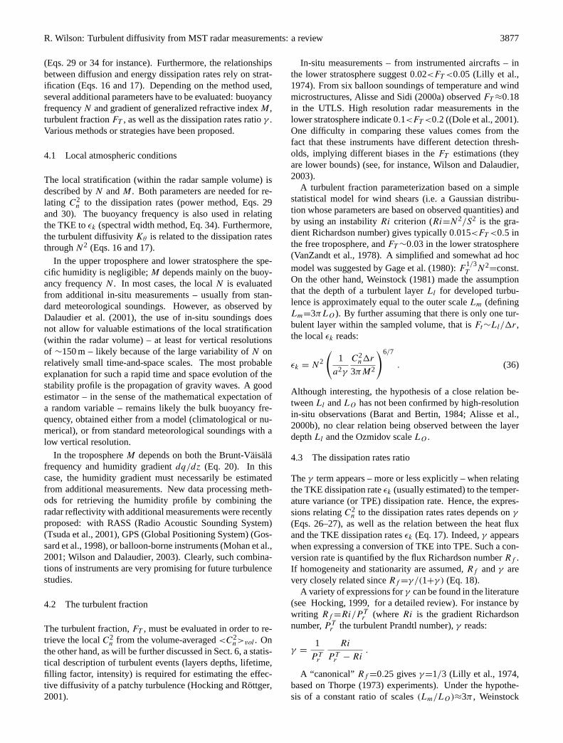
Fig. 4. The flux Richardson Number,Rf , versus the turbulent

Richardson number,Rio=N2L2m/q2 (observations and model),

from Rohr et al.(1984) andWeinstock(1992).

(1978) suggestsγ≈0.8. However, an accumulation of obser-vational evidences suggest thatγ is likely to be smaller than0.8 on the average (e.g.Weinstock, 1992). In fact, γ is ob-served to be significantly variable. Several estimations in theoceanic thermocline, lakes, or laboratory experiments (watertank) indicate 0.1<γ<0.4 (e.g.McEwan, 1983; Rohr et al.,1984; Gargett and Moum, 1995; Moum, 1996). In-situ andradar estimations in the UTLS indicate 0.06<γ<0.3 (Alisseand Sidi, 2000a; Dole et al., 2001).

Laboratory experiments (e.g.Rohr and Van Atta, 1987;Ivey and Imberger, 1991), direct numerical simulations (e.g.Smyth et al., 2001) or theoretical considerations (Weinstock,1992), suggest thatRf (and thusγ ) evolves during the lifecycle of the turbulence event. It is usually observed thatRf

is decreasing with decreasingRi0, the turbulent Richardsonnumber (Ri0=N2L2

m/q2 expresses the ratio of TPE to TKE).Weinstock(1992), giving up the hypothesis of a constant ra-tio of scales (Lm/LO ), suggests thatγ is a simple functionof Ri0 (Fig. 4):

γ ≈ 1.2Ri0 (for Ri0 ≤ 2) . (37)

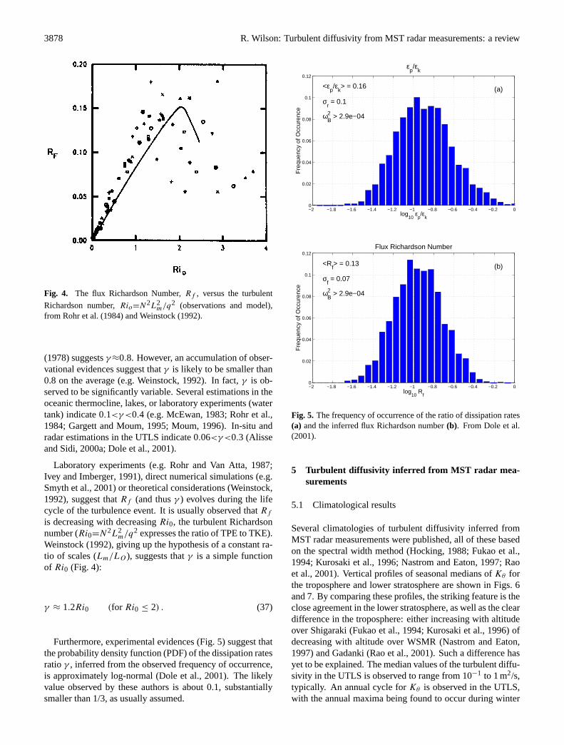
Furthermore, experimental evidences (Fig.5) suggest thatthe probability density function (PDF) of the dissipation ratesratioγ , inferred from the observed frequency of occurrence,is approximately log-normal (Dole et al., 2001). The likelyvalue observed by these authors is about 0.1, substantiallysmaller than 1/3, as usually assumed.

−2 −1.8 −1.6 −1.4 −1.2 −1 −0.8 −0.6 −0.4 −0.2 00

0.02

0.04

0.06

0.08

0.1

0.12

log10

εp/ε

k

Fre

quen

cy o

f Occ

uren

ce

εp/ε

k

<εp/ε

k> = 0.16

σr = 0.1

ωB2 > 2.9e−04

(a)

−2 −1.8 −1.6 −1.4 −1.2 −1 −0.8 −0.6 −0.4 −0.2 00

0.02

0.04

0.06

0.08

0.1

0.12

log10

Rf

Fre

quen

cy o

f Occ

uren

ce

Flux Richardson Number

<Rf> = 0.13

σf = 0.07

ωB2 > 2.9e−04

(b)

Fig. 5. The frequency of occurrence of the ratio of dissipation rates(a) and the inferred flux Richardson number(b). FromDole et al.(2001).

5 Turbulent diffusivity inferred from MST radar mea-surements

5.1 Climatological results

Several climatologies of turbulent diffusivity inferred fromMST radar measurements were published, all of these basedon the spectral width method (Hocking, 1988; Fukao et al.,1994; Kurosaki et al., 1996; Nastrom and Eaton, 1997; Raoet al., 2001). Vertical profiles of seasonal medians ofKθ forthe troposphere and lower stratosphere are shown in Figs.6and7. By comparing these profiles, the striking feature is theclose agreement in the lower stratosphere, as well as the cleardifference in the troposphere: either increasing with altitudeover Shigaraki (Fukao et al., 1994; Kurosaki et al., 1996) ofdecreasing with altitude over WSMR (Nastrom and Eaton,1997) and Gadanki (Rao et al., 2001). Such a difference hasyet to be explained. The median values of the turbulent diffu-sivity in the UTLS is observed to range from 10−1 to 1 m2/s,typically. An annual cycle forKθ is observed in the UTLS,with the annual maxima being found to occur during winter


(a) (b)

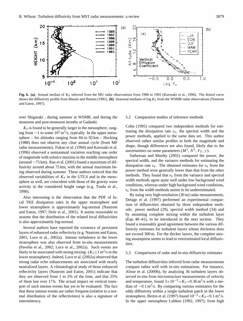
Fig. 6. (a): Annual median ofKθ inferred from the MU radar observations from 1986 to 1992 (Kurosaki et al., 1996). The dotted curveshows the diffusivity profile fromMassie and Hunten(1981). (b): Seasonal medians of logKθ from the WSMR radar observations (Nastromand Eaton, 1997).

over Shigaraki , during summer at WSMR, and during themonsoon and post-monsoon months at Gadanki.

Kθ is found to be generally larger in the mesosphere, rang-ing from∼1 to some 102 m2/s, typically. In the upper meso-sphere – for altitudes ranging from 84 to 92 km –Hocking(1988) does not observe any clear annual cycle (from MFradar measurements).Fukao et al.(1994) andKurosaki et al.(1996) observed a semiannual variation reaching one orderof magnitude with solstice maxima in the middle mesosphere(around∼75 km).Rao et al.(2001) found a maximum of dif-fusivity around about 75 km, with the annual maximum be-ing observed during summer. These authors noticed that theobserved variabilities ofKθ in the UTLS and in the meso-sphere as well, are coincident with those of the gravity waveactivity in the considered height range (e.g.Tsuda et al.,1990).

Also interesting is the observation that the PDF of lo-cal TKE dissipation rates in the upper stratosphere andlower stratosphere is approximately log-normal (Nastromand Eaton, 1997; Dole et al., 2001). It seems reasonable toassume that the distribution of the related local diffusivitiesis also approximately log-normal.

Several authors have reported the existence of persistentlayers of enhanced radar reflectivity (e.g.Nastrom and Eaton,2001; Luce et al., 2002a). Intense turbulence in the lowerstratosphere was also observed from in-situ measurements(Pavelin et al., 2002; Luce et al., 2002a). Such events arelikely to be associated with strong mixing: (Kθ≥1 m2/s in thelower stratosphere). Indeed,Luce et al.(2002a) observed thatstrong radar echo enhancements are associated with nearlyneutralized layers. A climatological study of those enhancedreflectivity layers (Nastrom and Eaton, 2001) indicate thatthey are observed from 1 to 2% of the time, and that 25%of them last over 17 h. The actual impact on vertical trans-port of such intense events has yet to be evaluated. The factthat these intense events are rather frequent (relative to a nor-mal distribution of the reflectivities) is also a signature ofintermittency.

5.2 Comparative studies of inference methods

Cohn (1995) compared two independent methods for esti-mating the dissipation rateεk, the spectral width and thepower methods, applied to the same data set. This authorobserved rather similar profiles in both the magnitude andshape, though differences are also found, likely due to theuncertainties on some parameters (M2, N2, FT , γ ).

Satheesan and Murthy(2002) compared the power, thespectral width, and the variance methods for estimating thedissipation rateεk. The obtained estimates forεk from thepower method were generally lower than that from the othermethods. They found thatεk from the variance and spectralwidth methods agree quite well under low background windconditions, whereas under high background wind conditions,εk from the width methods seems to be underestimated.

By using very high-resolution (30 m) radar measurements,Delage et al.(1997) performed an experimental compar-ison of diffusivities obtained by three independent meth-ods: power method (29), spectral width method (34) andby assuming complete mixing within the turbulent layer(Eqs.40–41), to be introduced in the next section. Theyfound a reasonably good agreement between the various dif-fusivity estimates for turbulent layers whose thickness doesnot exceed 300 m. For the thicker layers, the complete mix-ing assumption seems to lead to overestimated local diffusiv-ities.

5.3 Comparisons of radar and in-situ diffusivity estimates

The turbulent diffusivities inferred from radar measurementscompare rather well with in-situ estimations. For instance,Alisse et al.(2000b), by analyzing 36 turbulent layers ob-served in-situ from microstructure measurements of velocityand temperature, found 3×10−3<Kθ<0.36 m2/s with a me-dian of∼0.1 m2/s. By comparing various estimators for theeddy diffusivity within a single turbulent patch in the lowerstratosphere,Bertin et al.(1997) found 10−3<Kθ<0.1 m2/s.In the upper mesosphereLubken (1992, 1997), from high


(a) (b)

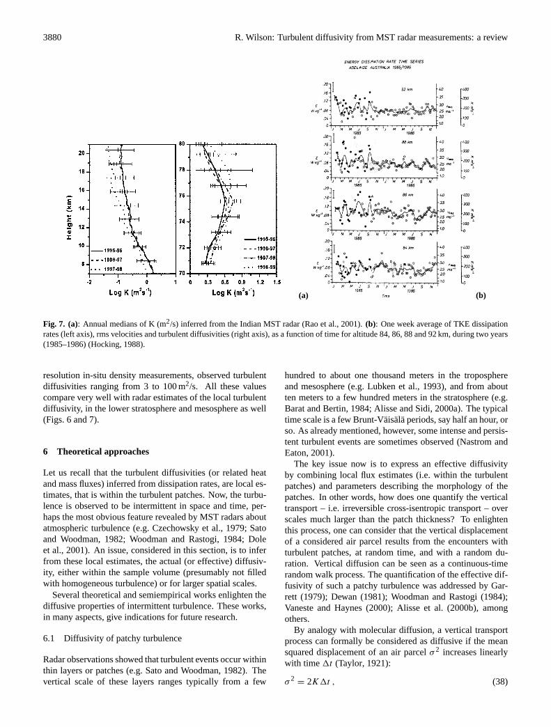
Fig. 7. (a): Annual medians of K (m2/s) inferred from the Indian MST radar (Rao et al., 2001). (b): One week average of TKE dissipationrates (left axis), rms velocities and turbulent diffusivities (right axis), as a function of time for altitude 84, 86, 88 and 92 km, during two years(1985–1986) (Hocking, 1988).

resolution in-situ density measurements, observed turbulentdiffusivities ranging from 3 to 100 m2/s. All these valuescompare very well with radar estimates of the local turbulentdiffusivity, in the lower stratosphere and mesosphere as well(Figs.6 and7).

6 Theoretical approaches

Let us recall that the turbulent diffusivities (or related heatand mass fluxes) inferred from dissipation rates, are local es-timates, that is within the turbulent patches. Now, the turbu-lence is observed to be intermittent in space and time, per-haps the most obvious feature revealed by MST radars aboutatmospheric turbulence (e.g.Czechowsky et al., 1979; Satoand Woodman, 1982; Woodman and Rastogi, 1984; Doleet al., 2001). An issue, considered in this section, is to inferfrom these local estimates, the actual (or effective) diffusiv-ity, either within the sample volume (presumably not filledwith homogeneous turbulence) or for larger spatial scales.

Several theoretical and semiempirical works enlighten thediffusive properties of intermittent turbulence. These works,in many aspects, give indications for future research.

6.1 Diffusivity of patchy turbulence

Radar observations showed that turbulent events occur withinthin layers or patches (e.g.Sato and Woodman, 1982). Thevertical scale of these layers ranges typically from a few

hundred to about one thousand meters in the troposphereand mesosphere (e.g.Lubken et al., 1993), and from aboutten meters to a few hundred meters in the stratosphere (e.g.Barat and Bertin, 1984; Alisse and Sidi, 2000a). The typicaltime scale is a few Brunt-Vaisala periods, say half an hour, orso. As already mentioned, however, some intense and persis-tent turbulent events are sometimes observed (Nastrom andEaton, 2001).

The key issue now is to express an effective diffusivityby combining local flux estimates (i.e. within the turbulentpatches) and parameters describing the morphology of thepatches. In other words, how does one quantify the verticaltransport – i.e. irreversible cross-isentropic transport – overscales much larger than the patch thickness? To enlightenthis process, one can consider that the vertical displacementof a considered air parcel results from the encounters withturbulent patches, at random time, and with a random du-ration. Vertical diffusion can be seen as a continuous-timerandom walk process. The quantification of the effective dif-fusivity of such a patchy turbulence was addressed byGar-rett (1979); Dewan(1981); Woodman and Rastogi(1984);Vaneste and Haynes(2000); Alisse et al.(2000b), amongothers.

By analogy with molecular diffusion, a vertical transportprocess can formally be considered as diffusive if the meansquared displacement of an air parcelσ 2 increases linearlywith time1t (Taylor, 1921):

σ 2= 2K1t , (38)


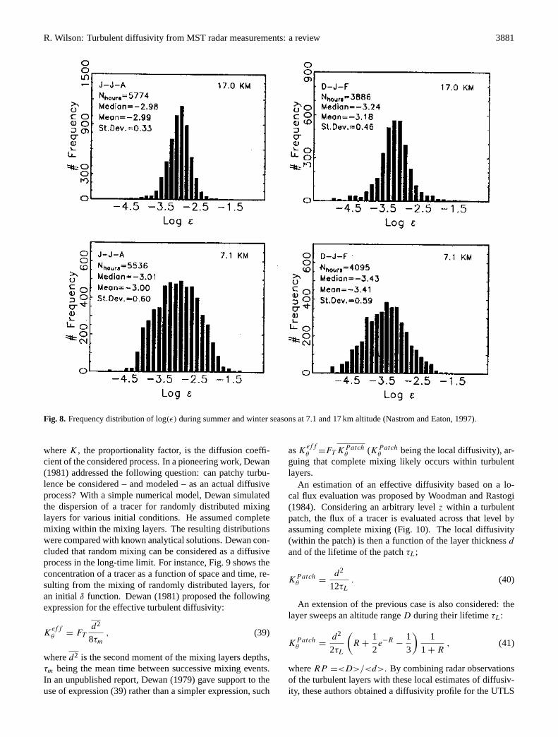
Fig. 8. Frequency distribution of log(ε) during summer and winter seasons at 7.1 and 17 km altitude (Nastrom and Eaton, 1997).

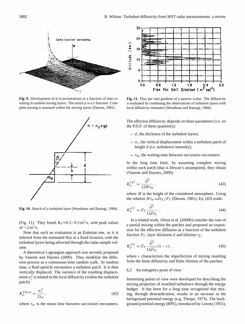
whereK, the proportionality factor, is the diffusion coeffi-cient of the considered process. In a pioneering work,Dewan(1981) addressed the following question: can patchy turbu-lence be considered – and modeled – as an actual diffusiveprocess? With a simple numerical model, Dewan simulatedthe dispersion of a tracer for randomly distributed mixinglayers for various initial conditions. He assumed completemixing within the mixing layers. The resulting distributionswere compared with known analytical solutions. Dewan con-cluded that random mixing can be considered as a diffusiveprocess in the long-time limit. For instance, Fig.9 shows theconcentration of a tracer as a function of space and time, re-sulting from the mixing of randomly distributed layers, foran initial δ function. Dewan(1981) proposed the followingexpression for the effective turbulent diffusivity:

Keffθ = FT

d2

8τm

, (39)

whered2 is the second moment of the mixing layers depths,τm being the mean time between successive mixing events.In an unpublished report,Dewan(1979) gave support to theuse of expression (39) rather than a simpler expression, such

asKeffθ =FT KPatch

θ (KPatchθ being the local diffusivity), ar-

guing that complete mixing likely occurs within turbulentlayers.

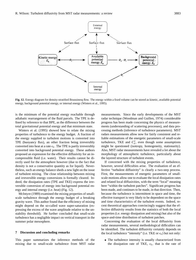
An estimation of an effective diffusivity based on a lo-cal flux evaluation was proposed byWoodman and Rastogi(1984). Considering an arbitrary levelz within a turbulentpatch, the flux of a tracer is evaluated across that level byassuming complete mixing (Fig.10). The local diffusivity(within the patch) is then a function of the layer thicknessd

and of the lifetime of the patchτL;

KPatchθ =

d2

12τL

. (40)

An extension of the previous case is also considered: thelayer sweeps an altitude rangeD during their lifetimeτL:

KPatchθ =

d2

2τL

(R +

1

2e−R

−1

3

)1

1 + R, (41)

whereRP =<D>/<d>. By combining radar observationsof the turbulent layers with these local estimates of diffusiv-ity, these authors obtained a diffusivity profile for the UTLS


Fig. 9. Development ofφ (concentration) as a function of time re-sulting in random mixing layers. The initialφ is aδ function. Com-plete mixing is assumed within the mixing layers (Dewan, 1981).

Fig. 10. Sketch of a turbulent layer (Woodman and Rastogi, 1984).

(Fig. 11). They foundKθ≈0.2−0.5 m2/s, with peak valuesof ∼2 m2/s.

Note that such an evaluation is an Eulerian one, as it isinferred from the estimated flux at a fixed location, with theturbulent layers being advected through the radar sample vol-ume.

A theoretical Lagrangian approach was recently proposedby Vaneste and Haynes(2000). They modelize the diffu-sion process as a continuous-time random walk. At randomtime, a fluid particle encounters a turbulent patch. It is thenvertically displaced. The variance of the resulting displace-mentσ 2

z is related to the local diffusivity (within the turbulentpatch):

KPatchθ =

σ 2z

2τm

, (42)

whereτm is the mean time between successive encounters.

Fig. 11. Flux per unit gradient of a passive scalar. The diffusivityis evaluated by combining the observations of turbulent layers withlocal diffusivity estimates (Woodman and Rastogi, 1984).

The effective diffusivity depends on three parameters (i.e. onthe P.D.F. of these quantities):

– d, the thickness of the turbulent layers;

– σz, the vertical displacement within a turbulent patch ofheightd (i.e. turbulence intensity);

– τm, the waiting time between successive encounters.

In the long time limit, by assuming complete mixingwithin each patch (that is Dewan’s assumption), they obtain(Vaneste and Haynes, 2000):

Keffθ =

d3

12Hτm

, (43)

whereH is the height of the considered atmosphere. Usingthe relationHτm=dτL/FT (Dewan, 1981), Eq. (43) reads:

Keffθ = FT

d3

12dτL

. (44)

In a related work,Alisse et al.(2000b) consider the case ofa partial mixing within the patches and proposed an expres-sion for the effective diffusion as a function of the turbulentfractionFT , layer thicknessd and lifetimeτL:

Keffθ = FT

d3

12dτL

(1 − c) , (45)

wherec characterizes the imperfection of mixing resultingfrom the finite diffusivity and finite lifetime of the patches.

6.2 An energetics point of view

Interesting points of view were developed for describing themixing properties of stratified turbulence through the energybudget. It has been for a long time recognized that mix-ing, through destratification, results in an increase in thebackground potential energy (e.g.Thorpe, 1973). The back-ground potential energy (BPE), introduced byLorenz(1955),


Fig. 12.Energy diagram for density-stratified Boussinesq flow. The energy within a fixed volume can be stored as kinetic, available potentialenergy, background potential energy, or internal energy (Winters et al., 1995).

is the minimum of the potential energy reachable throughadiabatic rearrangement of the fluid parcels. The TPE is de-fined by reference to that BPE, as the difference between thetotal gravitational potential energy and that minimum state.

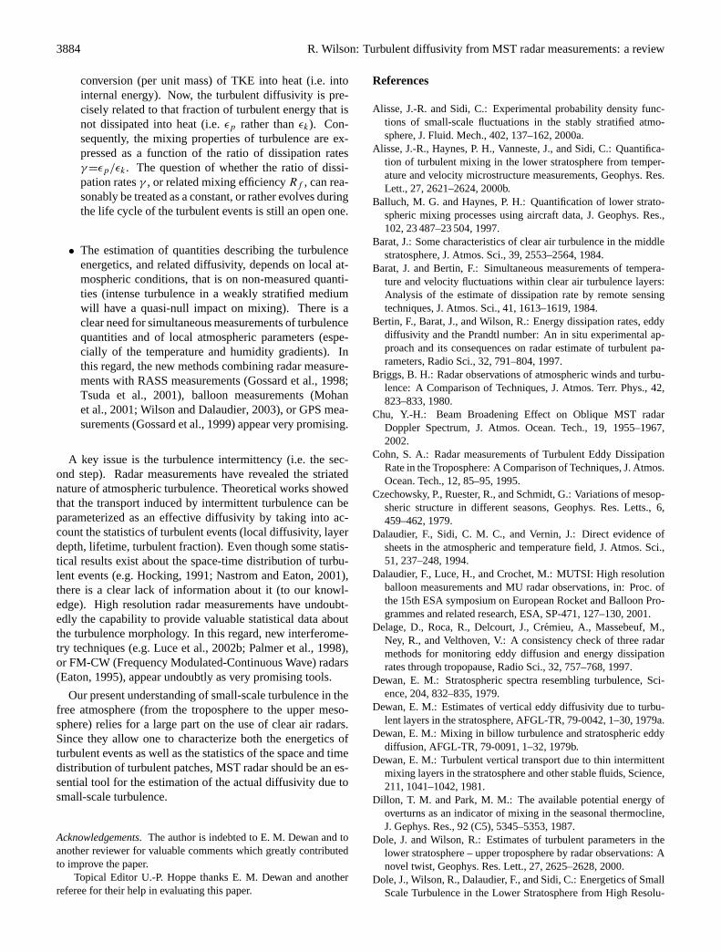
Winters et al.(1995) showed how to relate the mixingproperties of turbulence to the energy budget. A fraction ofthe energy supplied to turbulent motions is converted intoTPE (buoyancy flux), an other fraction being irreversiblyconverted into heat at a rateεk. The TPE is partly irreversiblyconverted into background potential energy. These authorsproposed an expression for the effective diffusivity for an in-compressible fluid (i.e. water). Their results cannot be di-rectly used for the atmosphere however (due to the fact thatdensity is not a conservative quantity as for liquid). Never-theless, such an energy balance sheds a new light on the issueof turbulent mixing. The close relationship between mixingand irreversible energy conversions is formally cleared. In-deed, the dissipation rates (TPE and TKE) express the irre-versible conversion of energy into background potential en-ergy and internal energy (i.e. heat) (Fig.12).

McIntyre(1989) examined the mixing properties of small-scale turbulence through the energy budget of a breakinggravity wave. This author found that the efficiency of mixingmight depend on the so-called wave super-saturation (ex-pressing the excess of the wave amplitude relative to the un-stability threshold). He further concluded that small-scaleturbulence has a negligible impact on vertical transport in thesummer polar mesosphere.

7 Discussion and concluding remarks

This paper summarizes the inference methods of themixing due to small-scale turbulence from MST radar

measurements. Since the early developments of the MSTradar technique (Woodman and Guillen, 1974) considerableprogress has been made concerning the physics of measure-ments (understanding of scattering processes), and data pro-cessing methods (inference of turbulence parameters). MSTradars measurements allow now for fairly consistent and re-liable estimations of the energetic parameters of small-scaleturbulence, TKE andC2

n, even though some assumptionsmight be questioned (isotropy, homogeneity, stationarity).Also, MST radar measurements have revealed a lot about themorphology of atmospheric turbulence, particularly aboutthe layered structure of turbulent events.

If concerned with the mixing properties of turbulence,however, several difficulties arise. The evaluation of an ef-fective “turbulent diffusivity” is clearly a two-step process.First, the measurements of energetic parameters of small-scale motions allow one to evaluate the local dissipation ratesand related local diffusivities, with the term “local” meaninghere “within the turbulent patches”. Significant progress hasbeen made, and continues to be made, in that direction. Then,because the turbulence is intermittent in space and time, theeffective transport is very likely to be dependent on the spaceand time characteristics of the turbulent events. Indeed, re-cent theoretical approaches convincingly suggest that the ef-fective diffusivity results from the statistics of both the localproperties (i.e. energy dissipation and mixing) but also of thespace-and-time distribution of turbulent patches.

Concerning the evaluation of the local diffusivity fromradar measurements, several methodological difficulties canbe identified. The turbulent diffusivity certainly depends onthe local turbulence “intensity” (i.e. TKE orεk) but not only:

• The turbulence intensity is usually characterized fromthe dissipation rate of TKE,εk, that is the rate of


conversion (per unit mass) of TKE into heat (i.e. intointernal energy). Now, the turbulent diffusivity is pre-cisely related to that fraction of turbulent energy that isnot dissipated into heat (i.e.εp rather thanεk). Con-sequently, the mixing properties of turbulence are ex-pressed as a function of the ratio of dissipation ratesγ=εp/εk. The question of whether the ratio of dissi-pation ratesγ , or related mixing efficiencyRf , can rea-sonably be treated as a constant, or rather evolves duringthe life cycle of the turbulent events is still an open one.

• The estimation of quantities describing the turbulenceenergetics, and related diffusivity, depends on local at-mospheric conditions, that is on non-measured quanti-ties (intense turbulence in a weakly stratified mediumwill have a quasi-null impact on mixing). There is aclear need for simultaneous measurements of turbulencequantities and of local atmospheric parameters (espe-cially of the temperature and humidity gradients). Inthis regard, the new methods combining radar measure-ments with RASS measurements (Gossard et al., 1998;Tsuda et al., 2001), balloon measurements (Mohanet al., 2001; Wilson and Dalaudier, 2003), or GPS mea-surements (Gossard et al., 1999) appear very promising.

A key issue is the turbulence intermittency (i.e. the sec-ond step). Radar measurements have revealed the striatednature of atmospheric turbulence. Theoretical works showedthat the transport induced by intermittent turbulence can beparameterized as an effective diffusivity by taking into ac-count the statistics of turbulent events (local diffusivity, layerdepth, lifetime, turbulent fraction). Even though some statis-tical results exist about the space-time distribution of turbu-lent events (e.g.Hocking, 1991; Nastrom and Eaton, 2001),there is a clear lack of information about it (to our knowl-edge). High resolution radar measurements have undoubt-edly the capability to provide valuable statistical data aboutthe turbulence morphology. In this regard, new interferome-try techniques (e.g.Luce et al., 2002b; Palmer et al., 1998),or FM-CW (Frequency Modulated-Continuous Wave) radars(Eaton, 1995), appear undoubtly as very promising tools.

Our present understanding of small-scale turbulence in thefree atmosphere (from the troposphere to the upper meso-sphere) relies for a large part on the use of clear air radars.Since they allow one to characterize both the energetics ofturbulent events as well as the statistics of the space and timedistribution of turbulent patches, MST radar should be an es-sential tool for the estimation of the actual diffusivity due tosmall-scale turbulence.

Acknowledgements.The author is indebted to E. M. Dewan and toanother reviewer for valuable comments which greatly contributedto improve the paper.

Topical Editor U.-P. Hoppe thanks E. M. Dewan and anotherreferee for their help in evaluating this paper.

References

Alisse, J.-R. and Sidi, C.: Experimental probability density func-tions of small-scale fluctuations in the stably stratified atmo-sphere, J. Fluid. Mech., 402, 137–162, 2000a.

Alisse, J.-R., Haynes, P. H., Vanneste, J., and Sidi, C.: Quantifica-tion of turbulent mixing in the lower stratosphere from temper-ature and velocity microstructure measurements, Geophys. Res.Lett., 27, 2621–2624, 2000b.

Balluch, M. G. and Haynes, P. H.: Quantification of lower strato-spheric mixing processes using aircraft data, J. Geophys. Res.,102, 23 487–23 504, 1997.

Barat, J.: Some characteristics of clear air turbulence in the middlestratosphere, J. Atmos. Sci., 39, 2553–2564, 1984.

Barat, J. and Bertin, F.: Simultaneous measurements of tempera-ture and velocity fluctuations within clear air turbulence layers:Analysis of the estimate of dissipation rate by remote sensingtechniques, J. Atmos. Sci., 41, 1613–1619, 1984.

Bertin, F., Barat, J., and Wilson, R.: Energy dissipation rates, eddydiffusivity and the Prandtl number: An in situ experimental ap-proach and its consequences on radar estimate of turbulent pa-rameters, Radio Sci., 32, 791–804, 1997.

Briggs, B. H.: Radar observations of atmospheric winds and turbu-lence: A Comparison of Techniques, J. Atmos. Terr. Phys., 42,823–833, 1980.

Chu, Y.-H.: Beam Broadening Effect on Oblique MST radarDoppler Spectrum, J. Atmos. Ocean. Tech., 19, 1955–1967,2002.

Cohn, S. A.: Radar measurements of Turbulent Eddy DissipationRate in the Troposphere: A Comparison of Techniques, J. Atmos.Ocean. Tech., 12, 85–95, 1995.

Czechowsky, P., Ruester, R., and Schmidt, G.: Variations of mesop-sheric structure in different seasons, Geophys. Res. Letts., 6,459–462, 1979.

Dalaudier, F., Sidi, C. M. C., and Vernin, J.: Direct evidence ofsheets in the atmospheric and temperature field, J. Atmos. Sci.,51, 237–248, 1994.

Dalaudier, F., Luce, H., and Crochet, M.: MUTSI: High resolutionballoon measurements and MU radar observations, in: Proc. ofthe 15th ESA symposium on European Rocket and Balloon Pro-grammes and related research, ESA, SP-471, 127–130, 2001.

Delage, D., Roca, R., Delcourt, J., Cremieu, A., Massebeuf, M.,Ney, R., and Velthoven, V.: A consistency check of three radarmethods for monitoring eddy diffusion and energy dissipationrates through tropopause, Radio Sci., 32, 757–768, 1997.

Dewan, E. M.: Stratospheric spectra resembling turbulence, Sci-ence, 204, 832–835, 1979.

Dewan, E. M.: Estimates of vertical eddy diffusivity due to turbu-lent layers in the stratosphere, AFGL-TR, 79-0042, 1–30, 1979a.

Dewan, E. M.: Mixing in billow turbulence and stratospheric eddydiffusion, AFGL-TR, 79-0091, 1–32, 1979b.

Dewan, E. M.: Turbulent vertical transport due to thin intermittentmixing layers in the stratosphere and other stable fluids, Science,211, 1041–1042, 1981.

Dillon, T. M. and Park, M. M.: The available potential energy ofoverturns as an indicator of mixing in the seasonal thermocline,J. Gephys. Res., 92 (C5), 5345–5353, 1987.

Dole, J. and Wilson, R.: Estimates of turbulent parameters in thelower stratosphere – upper troposphere by radar observations: Anovel twist, Geophys. Res. Lett., 27, 2625–2628, 2000.

Dole, J., Wilson, R., Dalaudier, F., and Sidi, C.: Energetics of SmallScale Turbulence in the Lower Stratosphere from High Resolu-


tion Radar Measurements, Ann. Geophys., 19, 945–952, 2001.Doviak, R. J. and Zrnic, D. S.: Doppler radar and weather observa-

tions, Academic Press, second edn., 1993.Eaton, F. D.: A new frequency-modulated continuous wave radar

for studying planetary boundary layer morphology, Radio Sci-ence, 30 (1), 75–88, 1995.

Eaton, F. D. and Nastrom, G. D.: Preliminary estimates of the ver-tical profiles of inner and outer scales from White Sands MissileRange, New Mexico, VHF radar observation, Radio Science, 33,895–903, 1998.

Fernando, H. J. S.: Environmental Stratified Flows, chap. Turbu-lence in Stratified Fluid, Kluwer Academic Publishers, 2002.

Frehlich, E.: Laser scintillation measurements of the temperaturespectrum in the atmospheric surface layer, J. Atmos. Sci., 49,1494–1509, 1992.

Frisch, A. S. and Clifford, S. F.: A study of convection capped bya stable layer using Doppler radar and acoustic echo sounder, J.Atmos. Sci., 31, 1622–1428, 1974.

Fukao, S., Yamanaka, M., Ao, N., Hocking, W. K., Sato, T., Ya-mamoto, M., Nakamura, T., Tsuda, T., and Kato, S.: Seasonalvariability of vertical diffusivity in the middle atmosphere, 1.Three-year observations by the middle and upper atmosphereradar, J. Geophys. Res., 99, 18 973–18 987, 1994.

Gage, K. S.: Evidence for ak−5/3 law inertial range in mesoscaletwo-dimensional turbulence, J. Atmos. Sci., 36, 1950–1954,1979.

Gage, K. S., Green, J. L., and VanZandt, T. E.: Use of Doppler radarfor the measurement of atmospheric turbulence parameters fromthe intensity of clear air echo, Radio Sci., 15, 407–416, 1980.

Gargett, A. E. and Moum, J. N.: Mixing efficiencies in turbulenttidal fronts: results from direct and indirect measurements ofdensity fluxes, J. Phys. Oceanogr., 25, 2583–2608, 1995.

Garrett, C.: Mixing in the ocean interior, Dyn. Atm. Oceans, 3,239–265, 1979.

Gill, A.: Atmosphere-Ocean Dynamics, Academic Press, 1982.Gossard, E. E. and Strauch, R. G.: Doppler radar and weather obser-

vations, Developments in Atmospheric Science, Elsevier, 1983.Gossard, E. E., Wolfe, D. E., Moran, K. P., Paulus, R. A., Anderson,

K. D., and Rogers, L. T.: Measurements of clear-air gradients andturbulence properties with radar wind profilers, J. Atmos. Ocean.Tech., 15, 321–342, 1998.

Gossard, E. E., Gutman, S., Stankov, B. B., and Wolf, D. E.: Profilesof radio refractive index and humidity derived from radar windprofilers and Global Positioning System, Radio Sci., 34 (2), 371–383, 1999.

Hall, C. M., Hope, U.-P., Blix, T. A., Thrane, E. V., H., M. A., andMeek, C. E.: Seasonal variation of turbulent energy dissipationrates in the polar mesosphere: a comparison of methods, EarthPlannets Space, 51, 515–524, 1999.

Hall, C. M., Nozawa, S., Manson, A. H., and Meek, C. E.: Deter-mination of turbulent energy dissipation rate directly from MF-radar determined velocity, Earth Plannets Space, 52, 137–141,2000.

Hill, R. J.: Spectra of fluctuations in refractivity, temperature, hu-midity, and the temperature-humidity cospectrum in the inertialand dissipation range, Radio Sci., 13, 953–961, 1978.

Hocking, W. K.: On the extraction of atmospheric turbulence pa-rameter from radar backscatter Doppler spectra – I. Theory, J.Atmos Terr. Phys., 45, 89–102, 1983.

Hocking, W. K.: Measurement of turbulent energy dissipation ratesin the middle atmosphere by radar techniques : A review, RadioSci., 20, 1403–1422, 1985.

Hocking, W. K.: Two years of continuous measurements of tur-bulence parameters in the upper mesosphere and lower thermo-sphere made with a 2-MHz radar, J. Gephys. Res., 91, 2475–2491, 1988.

Hocking, W. K.: The effects of middle atmospheric turbulence oncoupling between atmospheric regions, J. Geomag. Geoelectr.,43, suppl., 621–636, 1991.

Hocking, W. K.: An assessment of the capabilities and limitationsof radars in measurements of upper atmosphere turbulence, Adv.Space Res., 17 (11), 37–47, 1997.

Hocking, W. K.: The dynamical parameters of turbulence theory asthey apply to middle atmosphere studies, Earth Planets Space,51, 525–541, 1999.

Hocking, W. K. and Mu, K. L.: Upper and middle tropospheric ki-netic energy dissipation rates from measurements ofC2

n – reviewof theories, in-situ investigations, and experimental studies usingthe Buckland Park atmospheric radar in Australia, J. Atmos. Sol.Terr. Phys., 59, 1779–1803, 1997.

Hocking, W. K. and Rottger, J.: The structure of turbulence in themiddle and lower atmosphere seen by and deduced from MF, HF,and VHF radar, with special emphasis on small-scale featuresand anysotropy, Ann. Geophys., 19, 933–944, 2001.

Hocking, W. K., Fukao, S., Tsuda, T., Yamamoto, M., Sato, T.,and Sato, K.: Aspect sensitivity of stratospheric VHF radio wavescatterers, particularly above 15 km altitude, Radio Sci., 25, 613–627, 1990.

Hooper, D. and Thomas, L.: Aspect sensitivity of VHF scatterersin the troposphere and stratosphere from comparisons of powersin off-vertical beams, J. Atmos. Solar-Terr. Phys., 57, 655–663,1995.

Ivey, G. and Imberger, J.: On the nature of turbulence in a stratifiedfluid, Part 1: The energetics of mixing, J. Phys. Oceanogr., 21,650–658, 1991.

Kennedy, P. J. and Shapiro, M. A.: Further Encounters with ClearAir Turbulence in Research Aircraft, J. Atmos. Sci., 37, 986–993,1980.

Kurosaki, S., Yamanaka, M. D., Hashiguchi, H., Sato, T., andFukao, S.: Vertical eddy diffusivity in the lower and middle at-mosphere: a climatology based on the MU radar observationsduring 1986-1992, J. Atmos. Sol. Terr. Phys., 58, 727–734, 1996.

Legras, B., Joseph, B., and Lefevre, F.: Vertical diffusivity in thelower stratosphere from Lagrangian back-trajectory reconstruc-tion of ozone profiles, J. Geophys. Res., 108(D18), 4562, 2003.

Lilly, D. K., Waco, D. E., and Aldefang, S. I.: Stratospheric mixingestimated from high altitude turbulence measurements, J. Appl.Meteorol., 13, 488–493, 1974.

Lindborg, E.: Can the atmospheric kinetic energy spectrum be ex-plained by two-dimensional turbulence?, J. Fluid. Mech., 388,259–288, 1999.

Lorenz, E. N.: Available potential energy and the maintenance ofthe general circulation, Tellus, 7, 157–167, 1955.

Lubken, F.-J.: On the extraction of turbulent parameters from atmo-spheric density fluctuations, J. Gephys. Res., 97, 20,385–20,395,1992.

Lubken, F.-J.: Seasonal variation of turbulent energy dissipationrates at high latitudes as determined by insitu measurementsof neutral density fluctuations, J. Gephys. Res., 102, 13,441–13,456, 1997.

Lubken, F.-J., Hillert, W., Lehmacher, G., and von Zahn, U.: Exper-iments revealing small impact of turbulence on the energy budgetof the mesosphere and lower thermosphere, J. Gephys. Res., 98,20 369–20 384, 1993.


Luce, H., Crochet, M., Dalaudier, F., and Sidi, C.: Interpretationof VHF ST radar vertical echo from in situ temperature sheetobservations, Radio Sci., 30, 1002–1025, 1995.

Luce, H., Dalaudier, F., Crochet, M., and Sidi, C.: Direct compar-ison between in situ and VHF and oblique radar measurementsof refractive index spectra: a new successful attempt, Radio Sci.,31, 1487–1500, 1996.

Luce, H., Fukao, S., Dalaudier, F., and Crochet, M.: Strong mix-ing events observed near the tropopause with the MU radar andhight-resolution Balloon techniques, J. Atmos. Sci., 59, 2885–2896, 2002a.

Luce, H., Yamamoto, M., Fukao, S., Helal, D., and Crochet, M.: Afrequency domain radar interferometric imaging (FII) techniquebased on high-resolution methods, J. Atmos. Sol. Terr. Phys., 61,2885–2896, 2002b.

Manson, A. H., Meek, C. E., and Gregory, J. B.: Gravity wavesof short period (5-90 min) in the lower thermosphere at 52◦ N(Saskatoon, Canada): 1978/1979, J. Atmos. Terr. Phys., 43, 35–44, 1981.

Massie, S. T. and Hunten, D. M.: Stratospheric eddy diffusion coef-ficients from tracer data, J. Geophys. Res., 86, 9859–9868, 1981.

McEwan, A. D.: Internal mixing in stratified fluids, J. Fluid. Mech.,128, 59–80, 1983.

McIntyre, M. E.: On Dynamics and Transport Near the PolarMesopause in Summer, J. Gephys. Res., 94 (D12), 14 617–14 628, 1989.

Mohan, K., Narayama Rao, D., Narayama Rao, T., and Raghavan,S.: Estimation of temperature and humidity from MST radar ob-servation, Ann. Geophys., 19, 855–861, 2001.

Moum, J. N.: Efficiency of mixing in the main thermocline, J.Gephys. Res., 101, 12 057–12 069, 1996.

Nastrom, G. D. and Eaton, F. D.: Tubulence eddy dissipationrates from radar observations at 5–20 km at White Sands Mis-sile Range, New Mexico, J. Geophys. Res, 102, 19 495–19 505,1997.

Nastrom, G. D. and Eaton, F. D.: Persistent Layers of EnhancedC2n

in the Lower Stratosphere from VHF Radar Observations, RadioSci., 36, 137–149, 2001.

Nastrom, G. D. and Gage, K. S.: A climatology of atmosphericwavenumber spectra of wind and temperature observed by com-mercial aircraft, J. Atmos. Sci., 42, 950–960, 1985.

Nastrom, G. D. and Tsuda, T.: Anisotropy of Doppler spectralparmeters in the VHF radar observations at MU and WhiteSands, Ann. Geophys., 19, 883–888, 2001.

Ogawa, T. and Shimazaki, T.: Diurnal vaaariations of old nitro-gen and ionic density in the mesosphere and lower thermosphere:Simultaneous solutions of photochemical-diffusion equations, J.Gephys. Res., 80, 3945–3960, 1975.

Osborn, T. R.: Estimates of the local rate of vertical diffusion fromdissipation measurements, J. Phys. Oceanogr., 10, 83–89, 1980.

Osborn, T. R. and Cox, C. S.: Oceanic fine structure, Geophys.Fluid. Dyn., 3, 321–345, 1972.

Ottersten, H.: Radar backscattering from the turbulent clear atmo-sphere, Radio Sci., 4, 1251–1255, 1969a.

Ottersten, H.: Mean vertical gradient of potential refractive indexin turbulent mixing and radar detection of CAT, Radio Sci., 4,1247–1249, 1969b.

Palmer, R. D., Gopalam, S., Yu, T. Y., and Fukao, S.: Coherent radarimaging using the Capon’s method, Radio Sci., 33, 1585–1598,1998.

Pavelin, E., Whiteway, J., Busen, R., and Hacker, J.: Airborneobservations of turbulence, mixing, and gravity waves in the

tropopause region, J. Geophys. Res., 107 (D10), 4084, 2002.Rao, D. N., Ratnam, M. V., Rao, T. N., and Rao, S. V.: Seasonal

variation of vertical eddy diffusivity in the troposphere, lowerstratosphere and mesosphere over a tropical station, Ann. Geo-phys., 19, 975–984, 2001.

Rohr, J. J. and Van Atta, C. W.: Mixing efficiency in stably stratifiedgrowing turbulence, J. Gephys. Res., 92, 5481–5488, 1987.

Rohr, J. J., Itsweire, E. C., and Van Atta, C. W.: Mixing efficiency instably stratified decaying turbulence, Geophys. Astrophys. Fluid.Dyn., 29, 221–236, 1984.

Roper, R. G.: Atmospheric turbulence in the meteor region, J.Gephys. Res., 71, 5785–5792, 1966.

Roper, R. G.: On the radar estimation of turbulence parameters in astably stratified atmosphere, Radio Sci., 35, 999, 2000.

Roper, R. G. and Brosnahan, J. W.: Imaging Doppler Interferometryand the measurement of atmospheric turbulence,, Radio Sci., 32,1137–1148, 1997.

Satheesan, K. and Murthy, R. F. K.: Turbulence parameters in thetropical troposphere and lower stratosphere, J. Gephys. Res., 107(D1), ACL 2 (1–13), 2002.

Sato, T. and Woodman, R. F.: Fine Altitude Resolution Observa-tions of Stratospheric Turbulent Layers by the Arecibo 430 MHzRadar, J. Atmos. Sci., 39, 2546–2552, 1982.

Sidi, C. and Dalaudier, F.: Turbulence in the stratified atmosphere:Recent theoretical developments and experimental results, Adv.Space Res, 10 (10), 25–36, 1990.

Smyth, W. D. and Moum, J. N.: Length scales of turbulence instably stratified turbulence, Phys. Fluids, 12, 1327–1342, 2000.

Smyth, W. D., Moum, J. N., and Caldwell, D. R.: The efficiency ofmixing in turbulent patches: Inferences from direct simulationsand microstructure observations, J. Phys. Oceanogr., 31, 1969–1992, 2001.

Tatarskii, V. I.: Wave Propagation in a Turbulent Medium,McGraw-Hill, 1961.

Tatarskii, V. I.: The effects of the turbulent atmosphere onwave propagation, Israel Program for Scientific Translations,Jerusalem, 1971.

Taylor, G. I.: Diffusion by continuous movements, Proc. LondonMath. Soc., 20, 196–212, 1921.

Tennekes, H. and Lumley, J.: A first course in Turbulence, MITPress, 1972.

Thorpe, S. A.: Turbulence in stably stratified fluids: a review of lab-oratory experiments, Bound.-Layer Meteorol., 5, 95–119, 1973.

Tsuda, T., Sato, T., Fukao, S., and Kato, S.: MU radar observa-tions of the aspect sensitivity of backscattered VHF echo powerin the troposphere and lower stratosphere, Radio Sci., 21, 971–980, 1986.

Tsuda, T., Murayama, Y., Yamamoto, M., Kato, S., and Fukao,S.: Seasonal variation of momentum flux in the mesosphere ob-served with the MU radar, Geophys. Res. Lett., 17, 725–728,1990.

Tsuda, T., VanZandt, T. E., and Saito, H.: Zenith-angle dependenceof VHF specular reflection echoes in the lower atmosphere, J.Atmos. Solar-Terr. Phys., 59, 761–775, 1997a.

Tsuda, T., Miyamoto, M., and Furumoto, J.: Estimation of a Hu-midity Profile Using Turbulence Echo Characteristics, J. Atmos.Ocean. Tech., 18, 1214–1222, 2001.

Vaneste, J. and Haynes, P. H.: Intermittent mixing in strongly strat-ified fluids as a random walk, J. Fluid. Mech., 411, 165–185,2000.

VanZandt, T. E.: A universal spectrum of buoyancy waves in theatmosphere, Geophys. Res. Lett., 9, 575–578, 1982.


VanZandt, T. E., Green, J. L., Gage, K. S., and Clarck, W. L.: Verti-cal profiles of refractivity turbulence structure constant: compar-ison of observations by the Sunset radar with a new theoreticalmodel, Radio Sci., 13, 819–829, 1978.

VanZandt, T. E., Clarck, W. L., Gage, K. S., Williams, C. R., andEcklund, W. L.: A dual-wavelength radar technique for measur-ing the turbulent energy dissipation rateε, Geophys. Res. Lett.,27, 2537–2540, 2000.

VanZandt, T. E., Nastrom, G. D., Furumoto, J., Tsuda, T., andClarck, W. L.: A dual-beamwidth radar method for measuring at-mospheric turbulent kinetic energy, Geophys. Res. Lett., 29 (12),1572–1575, 2002.

Watkins, B. J., Philbrick, C. R., and Balsley, B. B.: TurbulenceEnergy Dissipation Rates and Inner Scale Sizes from Rocket andRadar Data, J. Gephys. Res., 93 (D6), 17 009–17 014, 1988.

Waugh, D., Plumb, R. A., Elkins, J. W., et al.: Mixing on polarvortex air into middle latitudes as revealed by tracer-tracer scatterplots, J. Geophys. Res., 102, 13 119–13 134, 1997.

Weinstock, J.: On the theory of turbulence in the buyoancy subrangeof stably stratified flows, J. Atmos. Sci., 35, 634–649, 1978.

Weinstock, J.: Using radar to estimate dissipation rate in thin layerof turbulence, Radio Sci., 16, 1401–1406, 1981.

Weinstock, J.: Vertical diffusivity and overturning length in stablystratified turbulence, J. Gephys. Res., 97, 12,653–12,658, 1992.

Wilson, R. and Dalaudier, F.: Simultaneous observations of atmo-spheric turbulence in the lower stratosphere from balloon sound-ings and ST radar measurements, in: Proc. of the 10th MST radarworkshop, 2003.

Winters, K. B., Lombard, P. N., Riley, J. J., and d’Assaro, E. A.:Available potential energy and mixing in density stratified fluid,J. Fluid. Mech., 289, 115–128, 1995.

Woodman, R. F. and Guillen, A.: Radar observations of winds andturbulence in the stratosphere and mesosphere, J. Atmos. Sci.,31, 493–505, 1974.

Woodman, R. F. and Rastogi, P. K.: Evaluation of effective eddydiffusive coefficients using radar observations of turbulence inthe stratosphere, Geophys. Res. Lett., 11, 243–246, 1984.

Worthington, R. M. and Thomas, P. K.: Long-period unstablegravity-waves and associated VHF radar echoes, Ann. Geophys.,15, 813–822, 1997.

Worthington, R. M., Palmer, R. D., and Fukao, S.: An Investigationof Tilted Aspect-Sensitive Scatterers in the Lower Atmosphere,Using the MU and Aberystwyth VHF Radars, Radio Sci., 34,413–426, 1999a.

Worthington, R. M., Palmer, R. D., and Fukao, S.: Complete mapsof the aspect sensitivity of VHF atmospheric radar echoes, Ann.Geophys., 17, 1116–1119, 1999b.

Documents

Reading expRess Lesson sampLeR Level H (Grade 8), Lesson