Readme Supplement

Version 7.50

Disclaimer

Please read the following carefully:

This software and this document have been developed and checked for correctness and accuracy by SST Systems, Inc. (SST) and InfoPlant Technologies Pvt. Ltd. (InfoPlant). However, no warranty, expressed or implied, is made by SST and InfoPlant as to the accuracy and correctness of this document or the functioning of the software and the accuracy, correctness and utilization of its calculations.

Users must carry out all necessary tests to assure the proper functioning of the software and the applicability of its results. All information presented by the software is for review, interpretation, approval and application by a Registered Professional Engineer.

CAEPIPE is a trademark of SST and InfoPlant.

CAEPIPE Version 7.50, © 2016, SST Systems, Inc. and InfoPlant Technologies Pvt. Ltd. All Rights Reserved.

SST Systems, Inc. Tel: (408) 452-8111 1798 Technology Drive, Suite 236 Fax: (408) 452-8388 San Jose, California 95110 Email: info@sstusa.com USA www.sstusa.com InfoPlant Technologies Pvt. Ltd. Tel: +91-80-40336999 7, Crescent Road Fax: +91-80-41494967 Bangalore 560001 Email: iplant@vsnl.com India

Annexure A

Code Compliance

EN 13480-3 (2012)

Allowable Pressure

The allowable pressure for straight pipes is calculated from Equation 6.1-1 or 6.1-3 depending on the ratio between inner and outer diameter.

For 7.1/ io DD

eD

fzeP

o

2

For 7.1/ io DD

)1(

)1(2

2

a

afzP

where

P = allowable pressure

f = allowable stress

z = joint factor (input as material property in CAEPIPE)

e = nominal pipe thickness x [1 - mill tolerance %/100] - corrosion allowance “c”

(Any additional thickness required for threading, grooving, erosion, corrosion, etc. should be included in corrosion allowance in CAEPIPE)

Do = outside diameter

Di = inside diameter

oD

ea

21

For pipe bends the maximum allowable pressure is calculated using the equivalent pipe wall thickness eequi.

f

equit

ee

Where

)50.0/(

)25.0/(

DR

DRt f

R = radius of bend

For closely spaced miter bends, the allowable pressure is calculated from Equations 6.3.4-1 and 6.3.4-2.

)2/(

)(,

)tan643.0(min

2

rRr

rRfze

reer

fzeP

s

s

with 22.5

For widely spaced miter bends, the allowable pressure is calculated from Equations 6.3.4-1, 6.3.4-2 and 6.3.5-1

)2/(

)(,

)tan643.0(min

2

rRr

rRfze

reer

fzeP

s

s

with 22.5

)tan25.1(

2

reer

fzeP

with > 22.5

Where

r = mean radius of pipe = (D - t)/2

Rs = effective bend radius of the miter

= miter half angle

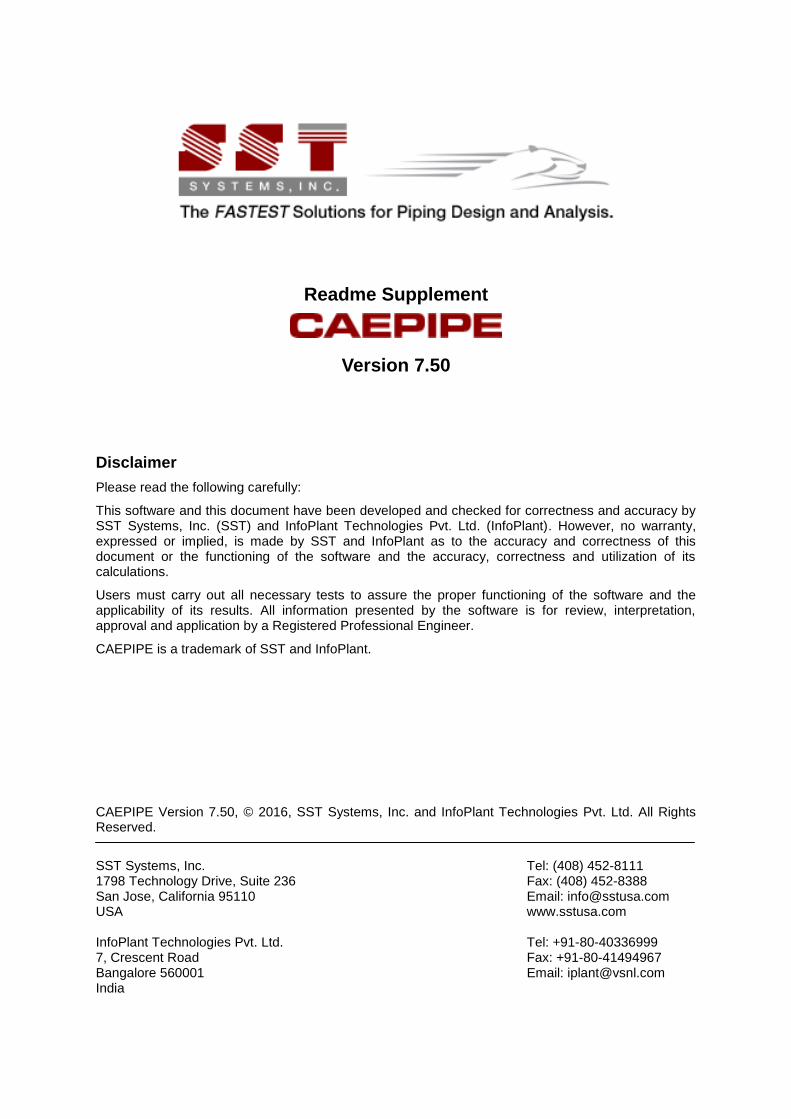
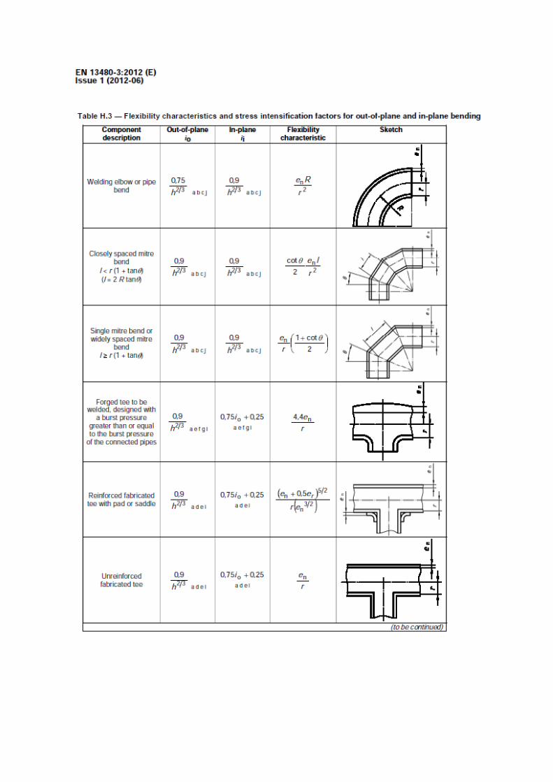
Sustained Stress

The stress ( 1 ) due to sustained loads (pressure, weight and other sustained mechanical loads) is

calculated from Equation (12.3.2-1)

fA

n

o fZ

iM

e

PD

75.0

41

where

P = maximum of CAEPIPE input pressures [i.e., max(P1 through P10)]

Do = outside diameter

en = nominal pipe thickness

i stress intensification factor; the product of 0.75i shall not be less than 1.0

AM resulting bending moment due to sustained loads

Z = uncorroded section modulus; for reduced outlets / branch connections, effective section modulus

ff = min(f; fcr) = design stress for flexibility analysis at the maximum operating temperature under consideration [i.e., max(T1 through T10)], where

f = min(Rp0.2t/1.5 ; Rm/2.4)

fcr = design stress in creep range at max(T1 through T10)

Rp0.2t = minimum 0.2% proof strength at max(T1 through T10)

Rm = Tensile Strength (= Tensile as shown in CAEPIPE material input)

Note:

Starting Version 7.50 of CAEPIPE, the value of “ff” is no longer input in the material properties table. Instead, the value of “f” which is calculated as min(Rp0.2t/1.5; Rm/2.4) is input for each temperature.

If a stress model created using an earlier version of CAEPIPE is read into Version 7.50 of CAEPIPE, then in the 7.50 model file, the material properties should be updated appropriately.

Sustained plus Occasional Stress

The stress ( 2 ) due to sustained and occasional loads is calculated from Equation (12.3.3-1) as the sum

of stress due to sustained loads such as due to pressure, weight and other sustained mechanical loads and stress due to occasional loads such as earthquake or wind. Wind and earthquake are not considered concurrently.

fBA

n

o kfZ

iM

Z

iM

e

PD

75.075.0

42

MB=resultant bending moment due to occasional load

k = 1.2 if the occasional load is acting less than 1% in any 24 hour operating period. In CAEPIPE, the default value of k is 1.2.

This k value can be modified through CAEPIPE Options > Analysis > Code > Occasional load factor.

Expansion Stress

The stress ( 3 ) due to thermal expansion is calculated from Equation (12.3.4-1)

aC f

Z

iM3

where

MC = resultant moment due to thermal expansion and alternating loads

Z = uncorroded section modulus; for reduced outlets / branch connections, effective section modulus

c

hhCa

E

EffUf )25.025.1( as per Equation (12.1.3-1)

U cyclic stress range reduction factor taken from Table 12.1.3-1

Ec = modulus of elasticity at the minimum metal temperature consistent with the loading under consideration

Eh = modulus of elasticity at the maximum metal temperature consistent with the loading under consideration

fC = min(Rm/3; f), where f = min(Rp0.2t/1.5 ; Rm/2.4) at room temperature (Tref) as per Equation (12.1.3-2)

fh = basic allowable stress at maximum metal temperature consistent with the loading under consideration = min(fc; f; fcr) as per Equation 12.1.3-3,

with fc determined at minimum metal temperature consistent with the loading under consideration and f determined at maximum metal temperature consistent with the loading under consideration

For example, for the thermal range (T1-T2), with T1 = 300 0C, T2 = 100

0C and Tref = 21

0C,

Ec is determined at T2 = 100 0C and Eh is determined at T1 =300

0C

fc as per Equation (12.1.3-2) listed above is determined at Tref = 21 0C,

the value of fc used in calculating fh is determined at T2 = 100 0C

the value of f used in calculating fh is determined at T1 = 300 0C and

the value of fcr is taken at T1 = 300 0C (if available)

If the above condition in Equation (12.3.4-1) is not met, Equation (12.3.4-2) may be used.

af

CA

n

o ffZ

iM

Z

iM

e

PD

75.0

44

Additional Conditions for the Creep Range

For piping operating within the creep range, the stress, 5 , due to sustained, thermal and alternating

loadings shall satisfy the Equation (12.3.5-1) below.

crCA

n

o fZ

iM

Z

iM

e

PD

3

75.075.0

45

where

crf = design stress in creep range at max(T1 through T10)

Stresses due to single non-repeated Support Movement (settlement)

Settlement evaluation as per Equation (12.3.6-1) of EN 13480-3 (2012) is not yet implemented in Version 7.50 of CAEPIPE.

Annexure B

Pressure Relief Valve Analysis

Pressure Relief Valve Analysis

A Simplified Approach

[Abbreviation: Pressure relief valve = PRV]

During an overpressure event, the discharge of a PRV imposes a load, referred to as a reaction force, on the collective installation. The flowrate and associated reaction force increase from nominally zero to some value, remain relatively constant at that value for the duration of the release, and then decrease to zero again, i.e., when the relief valve opens, the discharge fluid creates a jet force that acts on the piping system. This force increases from zero to its full value over a time frame similar to the opening time of the valve. The relief valve remains open until sufficient fluid is vented to relieve the overpressure situation. As the valve closes, the reduction in flow reduces the jet force to zero.

Detailed Analysis Approach

Perform a fluid transient analysis on the piping system using some software tool such as “FlowMaster”, “PipeNet”, “RELAP”, "ROLAST", etc.

Apply the resulting output obtained (forces as a function of time) at the bend node after the relief valve in a pipe stress analysis software (CAEPIPE).

Compute forces, moments and stresses in the piping system due to this loading.

As one can see, this method is detailed, time consuming and expensive.

Alternate Analysis Approach

American Petroleum Institute’s API 520, Part II, provides a basis for calculation of the reaction force in the event of a vapor or a two-phase release directly to the atmosphere. There is no discussion in this section of API 520, Part II, about the reaction force developed during a liquid release. Furthermore, no guidance is presented with respect to applying these results or determining if an installation is acceptable; instead, the burden is placed on the designer to ensure that the installation is appropriately designed. While this may be reasonable for the design of new facilities, evaluating the adequacy of existing facilities becomes much more complicated.

The formula (section 4.4.1.1) in US Customary units from API 520, Part II, for vapor relief devices discharging to the atmosphere, is shown below:

)()1(366

APMk

kTWF

where, F = Reaction force at the point of discharge to the atmosphere,(lbf.)

k = Ratio of specific heats (CP/CV) at the outlet conditions

W = Flow rate of any gas or vapor, pound mass (lbm.)/hr

CP = Specific heat at constant pressure

CV = Specific heat at constant volume

T = Temperature at the outlet, °R

M = Molecular weight of the process fluid

A = Area of the outlet at the point of discharge, in2

P = Static pressure within the outlet at the point of discharge, psig

Using the reaction force computed from the above formula along with the PRV parameters mentioned below:

Valve Opening Time

Valve Closing Time and

Relief duration (all obtained from the PRV manufacturer)

One can generate a PRV load profile and apply it in CAEPIPE for further analysis.

Example

By assuming the following data, one can apply the relief valve loading in CAEPIPE. Please see the model below for details.

1. Reaction force (F) computed = 6,700 lb.

2. Relief Valve Opening time = 8 ms (milliseconds)

3. Relief Valve Closing time = 8 ms

4. Relief duration = 1 s

5. Thermal Anchor Movement at Node 10 = 1” in (vertical) Y-direction

6. Pressure = 450 psig

7. Temperature = 650°F

A sample model, “ReliefValve.mod” is available with this document (and @ www.sstusa.com) for your reference. The steps followed in generating the model are given below.

After creating your piping model (with node 75 being the center node of the discharge bend where the PRV reaction force will be applied),

a. Select “Relief valve loading” from CAEPIPE Layout window > Misc and enter the data in the dialog box as shown in the figure below.

b. After entering the data as shown in the dialog above, press the button “OK”. This will generate a “Force Spectrum Load” as shown in the figure below.

c. Apply the Force Spectrum Load thus generated at the bend center node 75 after the relief valve in vertical direction (FY) as shown below.

d. Check “Force Spectrum” for analysis through Layout window > Load cases. Click on OK.

e. Save and Analyze the model.

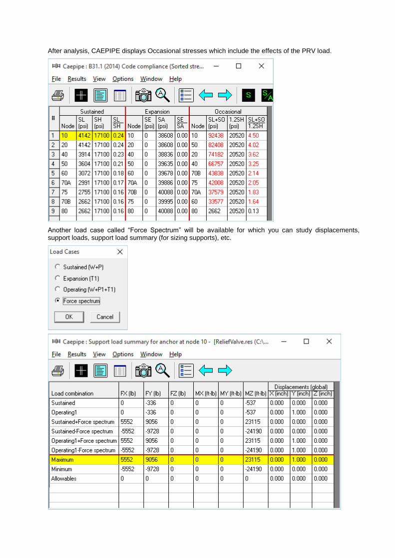
After analysis, CAEPIPE displays Occasional stresses which include the effects of the PRV load.

Another load case called “Force Spectrum” will be available for which you can study displacements, support loads, support load summary (for sizing supports), etc.

Annexure C

Generation of Mesh for Buried Piping Layout

(Automatic Discretization of Buried Piping Layout)

Generation of Mesh for Buried Piping Layout

Modulus of Subgrade Reaction (k)

This factor k defines the resistance of the soil or backfill to pipe movement due to the bearing pressure at the pipe/soil interface. Several methods for calculating modulus of subgrade reaction (k) have been developed in recent years.

As per Trautmann, C.H., and O’Rourke, T.D., “Lateral Force-Displacement Response of Buried Pipes,” Journal of Geotechnical Engineering, ASCE, Vol. 111, No. 9 Sep 1985, pp. 1077-1092, the modulus of subgrade reaction, k, can be calculated as per Eq. (2) in Appendix VII of ASME B31.1-2014 code.

wDNCk hk

where,

Ck = a dimensionless factor for estimating horizontal stiffness of compacted backfill. Ck may be estimated at 20 for loose soil, 30 for medium soil, and 80 for dense or compacted soil. In the current version of CAEPIPE, the value of Ck is internally set as 80 for both cohesive and cohesionless soil.

D = pipe outside diameter

w = soil density

Nh = a dimensionless horizontal force factor from Fig. 8 of above stated technical paper. For a typical value where the soil internal friction angle is 30 deg. the curve from Fig. 8 may be approximated by a straight line defined by

Nh = 0.285H/D + 4.3

where

H = the depth of pipe below grade at the pipe centerline

Influence Length (Lk)

The influence length is defined as the portion of a transverse pipe run which is deflected or “influenced” by pipe thermal expansion along the axis of the longitudinal run.

From Hetenyi’s theory, (Beams on Elastic Foundation, The University of Michigan Press, Ann Arbor, Michigan 1967) (also, see Section VII-3.3.2 of Appendix VII of ASME B31.1-2014 code)

4

3kL

where,

Pipe / Soil System Characteristics =

4/1

4

EI

k

E = modulus of elasticity of pipe at reference temperature

I = moment of inertia of pipe cross section

k = modulus of subgrade reaction of soil as detailed above.

Implementation in CAEPIPE

It is in the bends, elbows, and branch connections that the highest stresses are found in buried piping subjected to thermal expansion of the pipe. These stresses are due to the soil forces that bear against the transverse run. The stresses are proportional to the amount of soil deformation at the elbow or branch connection. Hence, piping element at the junction of bend, elbow and branch connection is to be refined in the stress layout.

This can be performed through Layout Window > Edit > Refine buried piping layout.

When the command is selected, CAEPIPE will refine the piping layout as detailed below.

1. Calculate modulus of subgrade reaction (k) as detailed above. While calculating k, the value of Ck is taken as 80 for both cohesive and cohesionless soil.

2. Calculate influence length (Lk) for the element that is fully buried.

3. If the length of the pipe element near bend / elbow / branch connection is greater than or equal to the influence length (Lk), then the pipe element will be split into a number of short elements with length of each short element being equal to 2 x OD of that pipe section until the Influence length (Lk).

On the other hand, if the length of the pipe element near bend / elbow / branch connection is less than the influence length (Lk) and greater than 2 x OD of the pipe, then the pipe element will be split into a number of short elements with length of each short element being equal to 2 x OD of that pipe section.

Note: while refining the layout, the new node number will be generated by adding the node increment specified (through Layout Window > Options > Node increment) to the available free node number. Hence, set the node increment value as required before refining the buried piping layout.

Sample buried piping model

The following data are used to generate the sample buried piping model.

Piping code = B31.1 (2014)

Use liberal allowable stresses

Do not include axial force in stress calculations

Reference temperature = 70 (F)

Number of thermal cycles = 7000

Number of thermal loads = 1

Thermal = Operating - Sustained

Use modulus at reference temperature

Include hanger stiffness

Include Bourdon effect

Use pressure correction for bends

Pressure stress = PD / 4t

Peak pressure factor = 1.00

Cut off frequency = 33 Hz

Number of modes = 20

Include missing mass correction

Use friction in dynamic analysis

Vertical direction = Y

-----------------------------------------------------------------------------------

Pipe material API: API 5L

-----------------------------------------------------------------------------------

Density = 0.283 (lb/in3), Nu = 0.300, Joint factor = 0.85, Type = CS

Temp E Alpha Allowable

(F) (psi) (in/in/F) (psi)

-------------------------------------------

-20 27.9E+6 6.25E-6 10900

100 27.9E+6 6.47E-6 10900

200 26.8E+6 6.70E-6 10900

300 25.3E+6 6.90E-6 10900

400 24.7E+6 7.10E-6 10900

-----------------------------------------------------------------------------------

Pipe Sections

-----------------------------------------------------------------------------------

Nominal O.D. Thk Cor.Al M.Tol Ins.Dens Ins.Th Lin.Dens Lin.Th

Name Dia. Sch (inch) (inch) (inch) (%) (lb/ft3) (inch) (lb/ft3) (inch)

-----------------------------------------------------------------------------------

12 12" STD 12.75 0.375 0 0.0

-----------------------------------------------------------------------------------

Soils

-----------------------------------------------------------------------------------

Name Type Density Strength Delta Ks Ground Level

(lb/ft3) (psi) (deg) (ft'in")

-----------------------------------------------------------------------------------

S1 Cohesionless 130 30 0.30 12'0"

-----------------------------------------------------------------------------------

Pipe Loads

-----------------------------------------------------------------------------------

Load T1 P1 T2 P2 T3 P3 Specific Add.Wgt Wind

Name (F) (psi) (F) (psi) (F) (psi) gravity (lb/ft) Load

-----------------------------------------------------------------------------------

L1 140 100

-----------------------------------------------------------------------------------

Soil characteristics

Soil density, w = 130 lb/ft3 = 0.075 lb/in3

Pipe depth below grade, H = 12 ft (144 in)

Type of backfill, dense sand (cohesion less soil)

Ck = 80

Calculation of Modulus of subgrade reaction (k)

Nh = 0.285H/D + 4.3

Nh = (0.285 x 144 / 12.75) + 4.3 = 7.518

wDNCk hk = 80 x 7.518 x 0.075 x 12.75 = 575.127 psi

Calculation of Influence Length (Lk)

Moment of inertia, I = 279.3 in4

Modulus of elasticity, E = 27.9 x 106 psi

4

3kL

Pipe / Soil System Characteristics =

4/1

4

EI

k = [575.127 / (4 x 27.9 x 106 x 279.3)]

1/4 = 0.01165

Influence Length (Lk) = 3 x 3.14 / (4 x 0.01165) = 202.145 in

As the length of pipe element near the bend and branch connection is greater than the influence length (Lk = 202.145 in), the pipe elements near the bends and branch connection are split into a number of short elements with length of each short element being equal to 2 x OD = 2 x 12.75 = 25.5 in until the influence length (Lk). See figures given below for details.