255

10. Reference Guide Formats and Conventions

The manual for the PLS_Toolbox uses a format consistent with that used for MATLAB. For additional information on usage see the above Functions section. The following format is used in the Reference section:

Purpose Provides short concise descriptions of a PLS_Toolbox command or function.

Synopsis Shows the input/output format of the command or function.

Description Describes what the command or function does and any rules or restrictions that apply.

Examples Provides examples of how the command or function can be used.

Options Describes advanced options of the command or function.

Algorithm Describes algorithms and routines used within the command or function.

See Also Refers to other related commands or functions in the PLS_Toolbox.

and the following conventions:

Monospace Commands, function names, and screen displays; for example, pca.

Italics Book titles, names of sections in this book, MATLAB toolbox names, and for introduction of new terms; for example, Chemometrics.

Monospace Optional input variables from PLS_Toolbox functions.

Routines in the PLS_Toolbox follow the convention of having samples in rows and variables in columns.

256

alignmat Purpose

Alignment of matrices and N-way arrays

Synopsis [bi,itst] = alignmat(amodel,b); [bi,itst] = alignmat(a,b,nocomp);

Description

In some cases, data arrays require alignment to aid the performance of the three-way (e.g. GRAM, or PARAFAC) or unfold models such as MPCA. For example, sometimes GC peaks or data from batch operations can be shifted on a sample-to-sample basis (each sample is a Mb by N matrix). In these cases, it is advantageous to choose a sub-matrix of a single matrix A as a standard and find the sub-matrix of subsequent samples B that best align or match the standard matrix. It is also possible to use a model of one or more standard matrices Amodel and find the sub-matrix of subsequent samples B that best align or match the model. In the latter case, it is also possible to find the sub-array of B that best aligns with the model of a N-way data set (Amodel). This can be performed along multiple modes using ALIGNMAT.

ALIGNMAT finds the subarray of b, bi, that most matches a using two different algorithms. For input: [bi,itst] = alignmat(amodel,b);

the sub-array bi is found using a projection method. In this case, bi is the sub-array of b that has the lowest residuals on a model of a called amodel. Models for amodel are standard model structures from PCA, PCR, GRAM, TLD, or PARAFAC. Input b can be class "double" or "dataset" and must have the same number of modes/dimensions as a with each element of size(b) ≥ size(a). Alignment is performed for modes with size(b) > size(a).

For input: [bi,itst] = alignmat(a,b,ncomp);

both a and b can be class "double" or "dataset", but both are two-way arrays (matrices). For a M by N then b must be Mb by N where Mb ≥ M (when Mb = M no alignment is performed). The output bi is the sub-array of b that best matches the matrix a. Optional input ncomp is a scalar of the number of components to use in the decomposition {default: ncomp = 1}.

Output bi is an array of class "double", itst is a cell array containing the indices of b that match bi. Note that since interpolation is used the indices in itst are not in general integers.

257

P

TMxN

MbxNb

Amodel

B

MbxNb

B

MxN

ABi

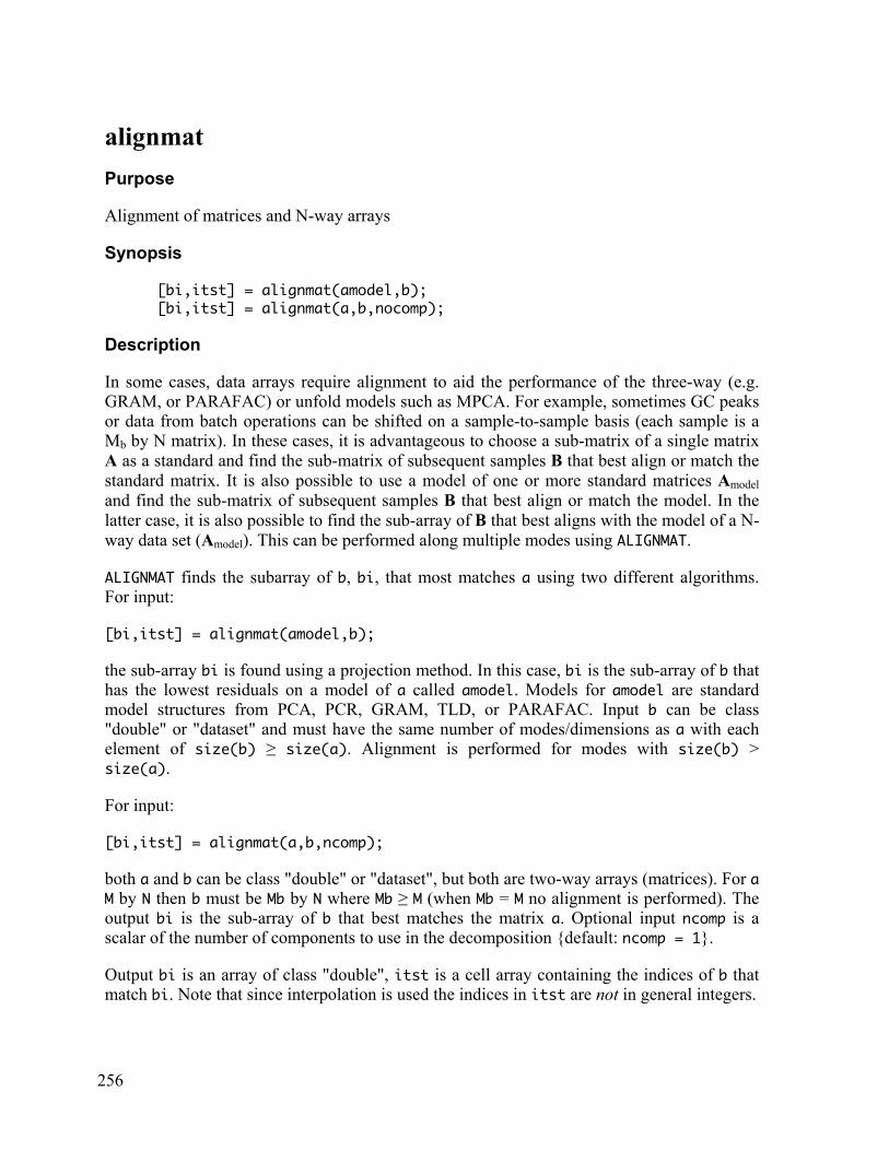
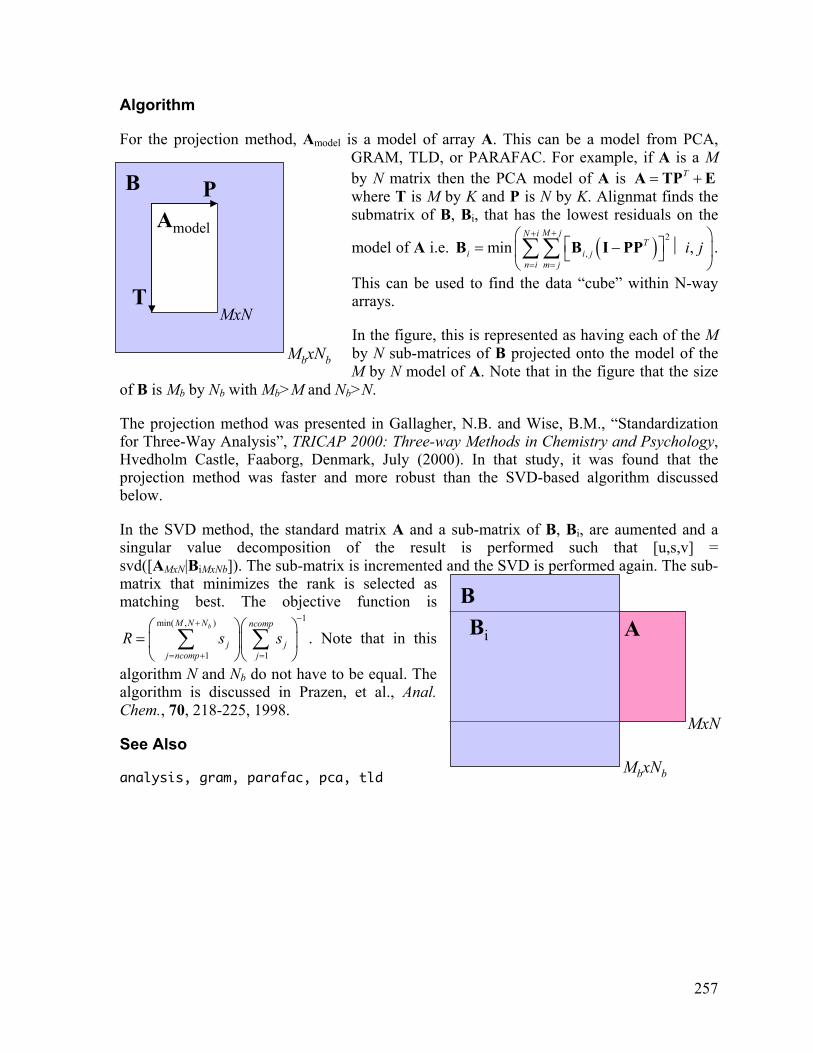
Algorithm

For the projection method, Amodel is a model of array A. This can be a model from PCA, GRAM, TLD, or PARAFAC. For example, if A is a M by N matrix then the PCA model of A is T= +A TP E where T is M by K and P is N by K. Alignmat finds the submatrix of B, Bi, that has the lowest residuals on the

model of A i.e. ( ) 2

,min ,M jN i

Ti i j

n i m ji j

++

= =

= − ∑ ∑B B I PP .

This can be used to find the data “cube” within N-way arrays.

In the figure, this is represented as having each of the M by N sub-matrices of B projected onto the model of the M by N model of A. Note that in the figure that the size

of B is Mb by Nb with Mb>M and Nb>N.

The projection method was presented in Gallagher, N.B. and Wise, B.M., “Standardization for Three-Way Analysis”, TRICAP 2000: Three-way Methods in Chemistry and Psychology, Hvedholm Castle, Faaborg, Denmark, July (2000). In that study, it was found that the projection method was faster and more robust than the SVD-based algorithm discussed below.

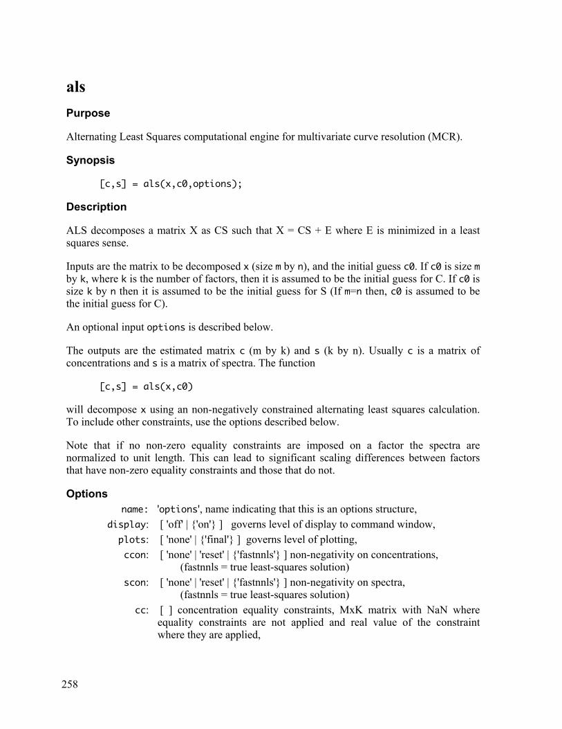
In the SVD method, the standard matrix A and a sub-matrix of B, Bi, are aumented and a singular value decomposition of the result is performed such that [u,s,v] = svd([AMxN|BiMxNb]). The sub-matrix is incremented and the SVD is performed again. The sub-matrix that minimizes the rank is selected as matching best. The objective function is

1min( , )

1 1

bM N N ncomp

j jj ncomp j

R s s−+

= + =

=

∑ ∑ . Note that in this

algorithm N and Nb do not have to be equal. The algorithm is discussed in Prazen, et al., Anal. Chem., 70, 218-225, 1998.

See Also

analysis, gram, parafac, pca, tld

258

als Purpose

Alternating Least Squares computational engine for multivariate curve resolution (MCR).

Synopsis [c,s] = als(x,c0,options);

Description

ALS decomposes a matrix X as CS such that X = CS + E where E is minimized in a least squares sense.

Inputs are the matrix to be decomposed x (size m by n), and the initial guess c0. If c0 is size m by k, where k is the number of factors, then it is assumed to be the initial guess for C. If c0 is size k by n then it is assumed to be the initial guess for S (If m=n then, c0 is assumed to be the initial guess for C).

An optional input options is described below.

The outputs are the estimated matrix c (m by k) and s (k by n). Usually c is a matrix of concentrations and s is a matrix of spectra. The function

[c,s] = als(x,c0)

will decompose x using an non-negatively constrained alternating least squares calculation. To include other constraints, use the options described below.

Note that if no non-zero equality constraints are imposed on a factor the spectra are normalized to unit length. This can lead to significant scaling differences between factors that have non-zero equality constraints and those that do not.

Options name: 'options', name indicating that this is an options structure, display: [ 'off' | {'on'} ] governs level of display to command window, plots: [ 'none' | {'final'} ] governs level of plotting, ccon: [ 'none' | 'reset' | {'fastnnls'} ] non-negativity on concentrations,

(fastnnls = true least-squares solution) scon: [ 'none' | 'reset' | {'fastnnls'} ] non-negativity on spectra,

(fastnnls = true least-squares solution) cc: [ ] concentration equality constraints, MxK matrix with NaN where

equality constraints are not applied and real value of the constraint where they are applied,

259

ccwts: [inf] weighting for equality constraints. Use inf for hard equality constraints and values < inf for soft equality constraints. Soft constraints weightings are given a fraction of the total sum-squared signal in X. If a scalar value is supplied, this value is used as the weighting for all factors. Otherwise, a vector K elements in length specifies the specific weighting to be use on each factor and may be a mix of hard (inf) and soft (<inf) constraints.

sc: [ ] spectral equality constraints, KxN matrix with NaN where equality constraints are not applied and real value of the constraint where they are applied,

scwts: [inf] weighting for spectral equality constraints (see ccwts) sclc: [ ] concentration scale axis, vector with M elements otherwise 1:M is

used, scls: [ ] spectra scale axis, vector with N elements otherwise 1:N is used, tolc: [ {1e-5} ] tolerance on non-negativity for concentrations, tols: [ {1e-5} ] tolerance on non-negativity for spectra, ittol: [ {1e-8} ] convergence tolerance, itmax: [ {100} ] maximum number of iterations, timemax: [ {3600} ] maximum time for iterations, rankfail: [ 'drop' |{'reset'}| 'random' | 'fail' ] how are rank deficiencies handled: drop - drop deficient components from model reset - reset deficient components to initial guess random - replace deficient components with random vector fail - stop analysis, give error

Examples

To decompose a matrix x without non-negativity constraints use: options = als(‘options’); options.ccon = ‘none’; options.scon = ‘none’; [c,s] = als(x,c0,options);

The following shows an example of using soft-constraints on the second spectral component of a three-component solution assuming that the variable softs contains the spectrum to which component two should be constrained.

[m,n] = size(x); options = als(‘options’); options.sc = NaN*ones(3,n); %all 3 unconstrained options.sc(2,:) = softs; %constrain component 2 options.scwts = 0.5; %consider as ½ of total signal in X [c,s] = als(x,c0,options);

See Also

260

pca, parafac

261

analysis Purpose

Graphical user interface for data analysis.

Synopsis analysis

Description

Performs various analysis methods including PCA, MCR, PARAFAC, Cluster, PLS, PCR, PLSDA, and SIMCA using a graphical user interface. Typical operations for file manipulation, preprocessing, and Analysis selection can be found in the menu items of the figure. Once data has been loaded and an Analysis selected, the Toolbar will populate with appropriate buttons for the Analysis. Plots created by the Toolbar buttons will bring up a plot figure window as well as a plot controls window. Use the plot controls window to manipulate the plot figure.

Note: For more information see Chapter 5 of the PLS_Toolbox Manual.

See Also

browse, cluster, mcr, parafac, pca, pcr, pls

262

anova1w Purpose

One way analysis of variance.

Synopsis anova1w(dat,alpha)

Description

Calculates one way ANOVA table and tests significance of between factors variation (it is assumed that each column of the data represents a different treatment). Inputs are the data table dat and the desired confidence level alpha, expressed as a fraction (e.g. 0.95, 0.99, etc.). The output is an ANOVA table written to the command window.

See Also

anova2w, ftest, statdemo

263

anova2w Purpose

Two way analysis of variance.

Synopsis anova2w(dat,alpha)

Description

Calculates two way ANOVA table and tests significance of between factors variation (it is assumed that each column of the data represents a different treatment) and between blocks variation (it is assumed that each row represents a block). Inputs are the data table dat and the desired confidence level alpha, expressed as a fraction (e.g. 0.95, 0.99, etc.). The output is an ANOVA table written to the command window.

See Also

anova1w, ftest, statdemo

264

areadr Purpose

Reads ASCII text file into workspace and strips off header.

Synopsis out = areadr1(file,nline,nvar,flag)

Description

Inputs are (file) an ASCII string containing the file name to be read, (nline) the number of rows to skip before reading, (nvar) the number of rows or columns in the matrix to be read, and (flag) which indicates whether (nvar) is the number of rows (flag=1) or the number of columns (flag=2) in the matrix.

AREADR can be incorporated into other routines to read data directly from groups of files. For example, to read the file mydata.txt with a 5 line header and 8 columns in the data into the matrix mymatrix:

mymatrix = areadr('mydata.txt',5,8,2)

See Also

spcreadr, xclreadr

265

auto Purpose

Autoscales a matrix to mean zero and unit variance.

Synopsis [ax,mx,stdx,msg] = auto(x,options) [ax,mx,stdx,msg] = auto(x,offset) options = auto('options')

Description

[ax,mx,stdx] = auto(x) autoscales a matrix x and returns the resulting matrix ax that has columns with mean zero and unit variance. Output mx is a vector of means, and stdx is a vector of standard deviations. mx and stdx can be used to scale new data (see SCALE).

Options options = a structure array with the following fields: name: 'options', name indicating that this is an options structure, offset: scaling can use standard deviation plus an offset {default = 0}, display: [ {'off'}| 'on' ] governs level of display to the command window, matrix_threshold: fraction of missing data allowed based on entire matrix (x) {default

= 0.15}, and column_threshold: fraction of missing data allowed base on a single column {default =

0.25}.

The optional input offset is added to the standard deviations before scaling and can be used to suppress low-level variables that would otherwise have standard deviations near zero.

The default options can be retreived using: options = auto('options');.

See Also

mncn, normaliz, scale, rescale

266

autocor Purpose

Calculates the autocorrelation function of a time series.

Synopsis acor = autocor(x,n,period,plots)

Description

acor = autocor(x,n) returns the autocorrelation function acor of a time series x for a maximum time shift of n sample periods.

acor = autocor(x,n,period) uses the sampling period period to scale the x-axis on the output plot. period can be empty [].

The optional input plots suppresses plotting if set to 0.

See Also

corrmap, crosscor

267

baseline Purpose

Subtracts a baseline offset from spectra.

Synopsis [newspec,b] = baseline(spec,freqs,range,options); spec = baseline(newspec,freqs,b,options);

Description

This function baselines spectra with a polynomial baseline function. The baseline function is fit to user-specified regions (regions free of peaks), which is then subtracted from the original spectra.

Inputs are spec class “double” or “dataset” containing the spectra, freqs the wavenumber or frequency axis vector, and range which specifies the baselining regions (see below). If freqs is omitted and spec is a dataset, the axissscale from the dataset will be used; otherwise a linear vector will be used.

range can be either an m by 2 matrix which specifies m baselining regions or a logical vector equal in length to the spectra with a 1 (one) at each point to be used as baseline and 0 (zero) elsewhere.

The output newspec contains the baselined spectra and b the polynomial coefficients.

If b is input instead of range with baselined spectra newspec then the output spec is a matrix original “unbaselined” spectra.

Options options = a structure array with the following fields: name: 'options', name indicating that this is an options structure, plots: [ {'none'} | 'final' ] governs plotting of results, and order: positive integer for polynomial order {default = 1}.

The default options can be retreived using: options = baseline('options');.

See Also

lamsel, normaliz, savgol, specedit

268

baselinew Purpose

Baseline using windowed polynomial filter.

Synopsis [y_b,b_b]= baselinew(y,x,width,order,res,options)

Description

BASELINEW recursivley calls LSQ2TOP to fit polynomials to the bottom (or top) of a curve e.g. a spectrum. It uses a windowed approach and can be considered a filter or baseline (low frequency) removal algorithm. The window depends on the frequency of the low frequency component (baseline) and wide windows and low order polynomials are often used. See LSQ2TOP.

The curve(s) to be fit (dependent variable) y, the axis to fit against (the independent variable) x [e.g. y = P(x)], the window width width (an odd integer), the polynomial order order, and an approximate noise level in the curve res. Note that y can be MxN where x is 1xN. The optional input options is discussed below.

Output y_b is a MxN matrix of ROW vectors that have had the baselines removed, and output b_b is a matrix of baselines. Therefore, y_b is the high frequency component and b_b is the low frequency component.

Examples

If y is a 5 by 100 matrix then y_b = baselinew(y,[],25,3,0.01);

gives a 5 by 100 matrix y_b of row vectors that have had the baseline removed using a 25-point cubic polynomial fit of each row of y.

If y is a 2 by 100 matrix then y_b = baselinew(y,x,51,3,0.01);

gives a 2 by 100 matrix y_b of row vectors that have had the baseline removed using a 51-point second order polynomial fit of each row of y to x.

Options options = structure array with the following fields: display : [ 'off' | {'on'} ] governs level of display to command window. trbflag : [ 'top' | {'bottom'} ] top or bottom flag, tells algorithm to fit the

polynomials, y = P(x), to the top or bottom of the data cloud.

269

tsqlim: [ 0.99 ] limit that governs whether a data point is significantly outside the fit residual defined by input res.

stopcrit: [1e-4 1e-4 1000 360] stopping criteria, iteration is continued until one of the stopping criterion is met: [(relative tolerance) (absolute tolerance) (maximum number of iterations) (maximum time [seconds])].

See Also

baseline, lamsel, lsq2top, mscorr, savgol, stdfir

270

browse Purpose

PLS_Toolbox Toolbar and Workspace browser.

Synopsis browse

Description

BROWSE provides a graphical interface for tools, variables and figures used by PLS_Toolbox. The default mode will display only tools (e.g. DataSet Editor, Decompose and Getting Started).

See Also

analysis, editds, helppls

271

calibsel Purpose

Stepwise variable selection (user contributed).

Synopsis channel = calibsel(x,y,alpha,flag)

Description

CALIBSEL performs the variable selection procedure described in Brown, P.J., Spiegelman, C.H., and Denham, M.C., “Chemometrics and spectral frequency selection”, Phil. Trans. R. Soc. Land. A 337, 311-322, (1991).

Inputs are the calibration spectra x and concentrations y, significance level for chi-square test alpha, and a variable flag that allows the user to modify how the routine iterates. The output channel is a vector of indices corresponding to selected channels/wavelengths in y.

See Also

fullsearch, gaselctr, genalg

272

cellne Purpose

Element by element comparison of two cells for inequality.

Synopsis out = cellne(c1,c2)

Description

CELLNE compares the two cell inputs, c1 and c2, for inequality. If the cell arrays are the same size, the corresponding cell elements are compared and a similarly sized array of logical (boolean) values, out, is returned. The array out contains a one if the two cell elements were not equal (different variable type or contents) and a zero if the two cell elements were equal.

If the cell sizes do not match, the function returns a single logical value of 1.

See Also

273

chilimit Purpose

Chi-squared confidence limits from sum-of-squares residuals.

Synopsis [lim,scl,dof] = chilimit(ssqr,cl) lim = chilimit(scl,dof,cl)

Description

CHILIMIT determines a confidence limit for sum-of-squares residuals, ssqr, by fitting the residuals to the g Chi-squared h distribution. If the sum-squared residuals are reasonably approximated by a Chi-squared distribution this gives a very good estimate of the confidence level. However, it has been observed that outliers can significantly bias the estimate.

The standard call to CHILIMIT uses the sum of squares residuals ssqr, and the optional fractional confidence level requested, cl {default = 0.95}. Outputs are the calculated limit lim, the scaling determined from the residuals scl, and the degrees of freedom determined from the residuals dof.

The scaling, scl, and number of degrees of freedom, dof, returned from a previous call to CHILIMIT can be used in subsequent calls to CHILIMIT to obtain new limits without the original residuals.

See Also

jmlimit, pca, pcr, pls, residuallimit

274

choosencomp Purpose

GUI to select number of components from a PCA sum-of-squares captured table.

Synopsis ncomp = choosencomp(model)

Description

The input model can be a standard PCA model structure or just a sum-of-squares (SSQ) captured table from a PCA model. CHOOSENCOMP creates a GUI that displays the SSQ table and allows the user to select the number of principal components (ncomp) from the list.

The returned value, ncomp, is the number of selected components or an empty value [] if the user selected Cancel in the GUI.

See Also

analysis, pca, pcaengine, simca

275

class2logical Purpose

Create a PLSDA logical block from class assignments.

Synopsis [y,nonzero] = class2logical(class,groups)

Description

Given a list of sample classes or a DataSet object with class assignments for samples (mode 1), CLASS2LOGICAL creates a logical array in which each column of y contains the logical class membership (i.e. 1 or 0) for each class. This logical block can be used as the input y in PLS or PCR to perform discriminate analysis. Similarly, the output can be used with crossval to perform PLSDA cross-validation. Classes can optionally be grouped together by providing class groupings.

Inputs are class a list of class assignments, or a dataset with classes for first mode, and groups an optional input containing either:

[1 2 3 …] a vector of classes to model OR

{[1 2] [3 4] ...} a cell array containing groups of classes to consider as one class. Each cell element will be one class (see e.g. below)

Any classes in class which are not listed in groups are considered part of no group and will be assigned zero for all columns in the output.

Outputs are y a logical array in which each column represents one of the classes in the input class list or one of the groups in groups and nonzero the indices of samples with non-zero class assignment.

Examples

(A) Given DataSet "arch" with classes 0-5, the following creates a logical block with two columns consisting of "true" only for class 3 in the first column and "true" only for class 2 in the second column.

y = class2logical(arch,[3 2])

(B) Given DataSet "arch" with classes 0-5, the following creates a logical block with two columns consisting of "true" only for classes 0 and 1 in the first column and "true" only for classes 2 and 4 in the second column.

y = class2logical(arch,{[1 0] [2 4]})Options

276

See Also

crossval, plsda, plsdthres

277

cluster Purpose

K-means and K-nearest neighbor cluster analysis with dendrograms.

Synopsis cluster(data,labels,options) cluster(data,options) options = cluster('options')

Description

cluster(data) performs a cluster analysis on data matrix data using K-means or K-nearest neighbor clustering and plots a dendrogram showing distances between the samples. data can be class “double” or “dataset”.

Optional input labels can be used to put labels on the dendrogram plots. For data M by N then labels must be a character array with M rows. When labels is not specified and data is class “double”, the dendrogram is plotted using sample numbers. When labels is not specified and data is class “dataset”, the dendrogram is plotted using sample labels. If the labels field is empty it will use sample numbers.

The output is a dendrogram showing the sample distances.

Note: Calling cluster with no inputs starts the graphical user interface (GUI) for this analysis method.

Options options = a structure array with the following fields: name: 'options', name indicating that this is an options structure, algorithm: [ {'knn'} | 'kmeans' ] clustering algorithm, preprocessing: {[]} Preprocessing structure or keyword (see PREPROCESS), pca: [ {'false'} | 'true' ] if ‘true’ then CLUSTER performs PCA first

and clustering on the scores, ncomp: [] number of PCA factors to use {default = [], the user is prompted to

select the number of factors from the SSQ table}, and mahalanobis: [ {'false'} | 'true' ] if ‘true’ then a Mahalanobis distance on the

scores is used.

The default options can be retreived using: options = cluster('options');.

See Also

gcluster

278

coadd Purpose

Reduce resolution through combination of adjacent variables or samples.

Synopsis databin = coadd(data,bins,options)

Description

COADD is used to combine ("bin") adjacent variables, samples, or slabs of a matrix. Inputs include the original array data, the number of elements to combine together bins {default: 2}, and an optional options structure options.

Unpaired values at the end of the matrix are padded with the least biased value to complete the bin. Output is the co-added data. Unlike DERESOLV, COADD reduces the size of the data matrix by a factor of 1/bins for the dimension.

Example

Given a matrix, data, size 300 by 1000, the following would coadd variables in groups of three:

databin = coadd(data,3);

and the following would coadd samples in groups of two: options.dim = 1; databin = coadd(data,2,options);

The following is equivalent to the previous two lines. databin = coadd(data,2,struct(‘dim’,1));

Options dim: Dimension in which to do combination {default = 2}, mode: [ 'sum' | {'mean'} | 'prod' ] method of combination.

Algorithm

The three modes, sum, mean and prod behave according to the following (described in terms of variables):

SUM: groups of variables are added together and stored. The resulting values will be larger in magnitude than the original values by a factor equal to the number of variables binned.

279

MEAN: groups of variables are added together and that sum is divided by the number of variables binned. The resulting values will be similar in magnitude to the original values.

PROD: groups of variables are multiplied together.

See Also

deresolv

280

coda_dw Purpose

Variable selection method for hyphenated methods with a mass spectropmeter as a detector. The variables (mass chromatograms) are selected on the basis of smoothness.

Synopsis [dw_value,dw_index] = coda_dw(data,level);

Description

CODA_DW the Durbin Watson values of the first derivative of the chromatograms in data. The optional argument level defines the limitit of Durbin Watson value used for a plot of the results. If level is an integer it is used to plot the best level chromatograms. Low values for Durbin Watson indicate good quality chromatograms. The Durbin Watson values (dw_values) as wel as their ranking indices (dw_index) (low to high, so good to low quality) . For more information the Durbin Watson method see the function DURBIN_WATSON.

data can be a matrix with the data or a datasetobject

Examples

Plotting the chromatograms with a Durbin Watson value less than 2.2.

coda_dw(data,2.2);

Plotting the best 40 chromatograms.

coda_dw(data,40);

Algorithm

The algorithm calculates the Durbin Watson values of the first derivative of the mass chromatograms.

See Also

durbin_watson

281

comparelcms_sim_interactive Purpose

Select variables that are different between related data sets, e.g. mass chromatograms from LC/MS data of different batches.

Synopsis comparelcms_sim_interactive

Description

COMPARELCMS_SIM_INTERACTIVE performs the variable (mass chromatogram) selection using comparelcms_simengine, but with added interactivity

See Also

comparelcms_simengine

282

comparelcms_simengine Purpose

Select variables that are different between related data sets, e.g. mass chromatograms from LC/MS data of different batches.

Synopsis y=comparelcms_simengine(data,filter_width)

Description

COMPARELCMS_SIMENGINE determines which variables are different between different data sets. For example, after applying coda_dw to LC/MS data sets of highly related samples, such as the data of a good and a bad batch, the results will be very similar. comparelcms_engine takes the next step and extracts the mass chromatograms that are different. This function is normally not called by itself but by the function comparelcms_sim_interactive. The input argument data is a data cube with mode 1 the number of samples, mode two the number of spectra and mode 3 the number of variables, The optional input argument filter_width is used to smooth the columns of the data set in order to minimize the effect of small shifts, The output argument y contains the similarity indices of the variables. Variables with a low similarity index show the differences between the data sets.

Examples

Determination of similarity indices with a filter of 7 data points. y=comparelcms_simengine(data,7)

Algorithm

The calculations are based on a similarity index of the minimum of the chromatograms (across the samples) and the maximum of the chromatograms.

See Also

comparelcms_sim_interactive

283

compressmodel Purpose

Remove references to unused variables from a model.

Synopsis [cmodel,msg] = compressmodel(model)

Description

COMPRESSMODEL will remove any references in a model to excluded variables. This permits the application of the model to new data in which unused variables have been hard-excluded (i.e. previously removed or not collected). Input is model the model to compress. Outputs are cmodel the compressed model and msg any warning messages reported during compression. Although compression will work on most models, some preprocessing methods and some model types may not compress correctly. In these cases, a warning will be given and reported in the output msg.

See Also

pca, pcr, pls, plsda

284

contrastmod Purpose

Increase the contrast in Image PCA models.

Synopsis cmod = contrastmod(mod,data,thresh)

Description

CONTRASTMOD is used to increase the contrast in imgae PCA models by trimming off scores that are far from the mean.

Inputs are the model from IMGPCA mod, and the original data used to build the model data.

Optional threshold in standard deviations thresh gives the cutoff point for the scores {default thresh = 2.5}.

See Also

imagegui, imgselct, imgpca, imgsimca, isimcapr

285

copydsfields Purpose

Copies informational fields between datasets and/or model structures.

Synopsis to = copydsfields(from,to,modes,block)

Description

Copies all informational fields from one dataset to another, one model structure to another, or between datasets and models. This function copies the fields: label, class, title, axisscale, and includ as well as the "<field>name" assosciated with each (e.g. classname). If copying to or from a model structure, the fields to be copied from/to are sub-fields of the detail field.

Inputs are: from the dataset or model from which fields should be copied, and to the dataset or model to which fields should be copied. Optional input modes, are the modes (dimensions) which should be copied {default: all modes}. modes can also be a cell of {[to_modes] [from_modes]} to allow cross-mode copying. Optional input block is the data block of model from/to which information should be copied. For datasets, block refers to the field set {default: block/set 1}. block can also be a cell of {[to_block] [from_block]} to allow cross-block/set copying.

Output is: to, the updated dataset or model.

Examples

mydataset2 = copydsfields(mydataset1, mydataset2);

copies all fields for all modes of mydataset1 into mydataset2 (copies set 1 only).

mydataset2 = copydsfields(modl, mydataset2, {2 1});

copies all fields from mode 2 (variables) of modl into mode 1 of mydataset2.

modl = copydsfields(mydataset,modl,1,{1 2});

copies all fields for mode 1 (samples) from set 1 of mydataset into block 2 (e.g. y-block) of modl.

See Also

dataset/dataset, modelstruct, pca, pcr, pls

286

corcondia Purpose

Evaluate consistency of PARAFAC model.

Synopsis CoreConsist = corcondia(X,loads,Weights,plots);

Description

PARAFAC can be written as a special Tucker3 model where the core is superdiagonal with ones on the diagonal. This special way of writing the model can be used to check the adequacy of a PARAFAC model by estimating what Tucker3 core is found if estimated unconstrained from the PARAFAC loadings. The core consistency is given as the percentage of variation in this core array consistent with the theoretical superdiagonal array. The maximum core consistency is thus 100%. Consistencies well below 70-90% indicate that either too many components are used or the model is otherwise mis-specified. The consistency can also become negative which means that the model is not reasonable. Note that core consistency is an ad hoc method. It often works well on real data, but not as well with simulated data. CORCONDIA does not provide proof of dimensionality, but it can give a good indication.

Inputs are the multi-way array X and loads which can be a) a cell array with PARAFAC model loadings or b) a PARAFAC model structure.

Optional inputs are Weights which can be used to update the core in a weighted least squares sence and plots which suppress plotting of the results when set to zero (0).

See Also

corecalc, parafac, tucker

287

coreanal Purpose

Evaluate, display, and rotate core from a Tucker model.

Synopsis result = coreanal(core,action,param)

Description

Performs an analysis of the input core array of a Tucker model core. Results are returned in the output result.

Optional input action is a text string used to customize the analysis.

When action = 'list', the output result contains text describing the main properties of the core. If coreanal is called without outputs, the text is printed to the command window. If optional input param is included, the number of core entries shown can be controlled.

When action = 'plot', the core array is plotted and output result is not assigned. If action = 'maxvar', the core is rotated to maximum variance. The output result is a structure array containing the rotated core in the field core and the rotation matrices to achieve this rotation in the field transformation.

The loadings of the Tucker model should also be rotated correspondingly which can also be done using coreanal.

Examples result = coreanal(model,'list'); result = coreanal(model.core,'list');

will list information on the core-entries (explained variance etc). result = coreanal(model.core,'list',10); coreanal(model.core,'list',10);

will do the same but only for the ten most significant core-entries with the second version (with no output) printing the information to the command window.

result = coreanal(model,'plot');

will make a plot of the core where the size of each core-entry shows the variance explained. If the core is of higher order than three, it is first rearranged to a three-way array.

rotatedcore = coreanal(model,'maxvar');

288

will rotate the core to maximal variance. rotatedmodel = coreanal(oldmodel,rotatedcore);

where the input oldmodel is the original Tucker model structure and rotatedcore is the output from above. The rotation can be achieved in one step using:

rotatedmodel = coreanal(oldmodel,coreanal(oldmodel,'maxvar'));

See Also

corecalc, tucker

289

corecalc Purpose

Calculates the Tucker3 core array given the data array and loadings

Synopsis Core = corecalc(X,loads,orth,Weights,OldCore);

Description

Caculates the core array given the data X and the loadings loads (component matrices) which are held in a cell (see TUCKER).

Optional input orth is set to 0 to tell CORECALC that the loadings are NOT orthogonal.

Optional input Weights allows a weighted least squares solution to be sought.

Optional input OldCore provides a prior estimate of the core to speed up calculations.

The output Core is the Tucker3 core.

See Also

corcondia, coreanal, parafac, tucker

290

corrmap Purpose

Correlation map with variable regrouping.

Synopsis order = corrmap(data,labels,reord) order = corrmap(data,reord)

Description

CORRMAP produces a pseudocolor map that shows the correlation between variables (columns) in a data set. The function will reorder the variables by KNN clustering if desired.

The input is the data data class "double" or "dataset".

Optional input labels contains the variable labels when the data is class "double".

Optional input reord will cause CORRMAP to keep the original ordering of the variables if set to 0.

The output order is a vector of indices with the variable ordering.

corrmap(data,labels) produces a psuedocolor correlation map with variable reordering.

corrmap(data,labels,0) produces a psuedocolor correlation map without variable reordering.

See Also

autocor, crosscor

291

cr Purpose

Continuum regression for multivariate y.

Synopsis b = cr(x,y,lv,powers)

Description

CR develops continuum regression models for a matrix of predictor variables (x-block) x, and vector or matrix of predicted variables (y-block) y. Models are calculated for 1 to lv latent variables for each value of the continuum parameter specified in the row vector powers. The output is the matrix of regression vectors b.

For a y-block with ny variables, x-block with nx variables, and np powers (size of powers is 1 by np) b is size (lv*ny*np) by nx. The first block in b corresponds to the first power in powers and is (lv*ny) by nx with the first row corresponding to a 1 latent variable model for the first y variable.

CR uses the de Jong, Wise & Ricker method for continuum regression (S. de Jong, B. M. Wise and N. L. Ricker, "Canonical Partial Least Squares and Continuum Power Regression," J. Chemo., 15, 85-100, 2001). It is a drastically faster implementation of the Wise and Ricker method used in the previous powerpls. Note that results are identical for both methods for the univariate y case but not for the multivariate y, where the results from CR are typically slightly better.

The algorithm used here is usually stable up to a continuum parameter of about 6-8, sometimes as high as 10 depending upon the problem. At powers this high, however, the models have essentially converged to the PCR solution. No instabilities at small powers have been noted.

See Also

crcvrnd, pcr, pls

292

crcvrnd Purpose

Cross-validation for continuum regression models using SDEP.

Synopsis [press,fiterr,mlvp,b] = crcvrnd(x,y,splt,itr,lv,pwrs,ss,mc)

Description

crcvrnd is used to cross-validate continuum regression models given a matrix of predictor variables (x-block) x, matrix or vector of predicted variables (y-block) y, the number of divisions into which to split the data splt, the number of iterations of the cross-validation procedure using different re-orderings of the data set itr, maximum number of latent variables lv and the row vector of continuum regression parameters to consider powers.

The outputs are the predictive residual error sum of squares (PRESS) matrix press where each element of the matrix represents the PRESS for a given combination of LVs and continuum parameter, the corresponding fit error fiterr, the number of LVs and power at minimum PRESS mlvp and the final regression vector or matrix b.

The optional input ss causes the routine to choose contiguous blocks of data during cross-validation when set to 1. If the optional input mc is set to 0 the subsets are not mean-centered during cross-validation.

A good smooth PRESS surface can usuall be obtained by calculating about 20 models spaced logarithmically between 4 and 1/4 and using 10 to 30 iterations of the cross-validation. A good rule of thumb for dividing the data is to use either the square root of the number of samples or 10, which ever is smaller.

See Also

cr, pcr, pls

293

crosscor Purpose

Calculates the crosscorrelation function of two time series.

Synopsis crcor = crosscor(x,y,n,period,flag,plots)

Description

crcor = crosscor(x,y,n) returns the crosscorrelation function crcor of two time series x and y for a maximum time shift of n sample periods.

crcor = crosscor(x,y,n,period) uses the sampling period period to scale the x-axis on the output plot.

crcor = crosscor(x,y,n,period,flag) with flag set to 1 changes the routine from cross correlation to cross covariance.

Optional input plots suppresses plotting when set to 0.

See Also

autocor, corrmap, wrtpulse

294

crossval Purpose

Cross-validation for PCA, PLS, MLR, and PCR.

Synopsis [press,cumpress,rmsecv,rmsec,cvpred,misclassed] = crossval(x,y,rm,cvi,ncomp,out,pre)

Description

CROSSVAL performs cross-validation for linear regression (PCR, PLS, MLR) and principal components analysis (PCA). Inputs are the predictor variable matrix x, predicted variable y (y is empty [] for rm = 'pca'), regression method rm, cross-validation method cvi, and maximum number of latent variables / components ncomp.

rm = 'pca' performs cross-validation for PCA, rm = 'mlr' performs cross-validation for MLR, rm = 'pcr' performs cross-validation for PCR, rm = 'nip' performs cross-validation for PLS using NIPALS, rm = 'sim' performs cross-validation for PLS using SIMPLS, and rm = 'lwr' performs cross-validation for LWR. cvi can be 1) a cell containing one of the cross-validation methods below with the appropriate parameters {cvm splits iter}, or 2) a vector representing user-defined cross-validation groups. cvi = {'loo'}; leave-one-out cross-validation, cvi = {'vet' splits}; venetian blinds, or cvi = {'con' splits}; contiguous blocks, and cvi = {'rnd' splits iter}; random subsets. Except for leave-one-out, all methods require the number of data splits splits to be provided. Random data subsets ('rnd') also requires number of iterations iter.

For user-defined cross-validation, cvi is a vector with the same number of elements as x has rows (i.e. length(cvi) = size(x,1); when x is class “double”, or length(cvi) = size(x.data,1); when x is class “dataset”) with integer elements, defining test subsets. Each cvi(i) is defined as:

cvi(i) = -2 the sample is always in the test set, cvi(i) = -1 the sample is always in the calibration set, cvi(i) = 0 the sample is always never used, and cvi(i) = 1,2,3… defines each subset.

295

Optional variable out suppresses plotting of the results when set to 0 {default = 1}. Optional variable pre is a cell defining preprocessing to be used on the x- and y-block respectively: {ppx ppy} where ppx and ppy are preprocessing structures (For more information see PREPROCESS). pre can also be a mean-centering flag; If pre is 0 then no preprocessing is done, if pre is 1, then mean centering is done on both blocks.

Outputs are the predictive residual error sum of squares (PRESS) press for each subset, the cumulative PRESS cumpress, the root mean square error of cross validation RMSECV rmsecv, the root mean square error of calibration RMSEC rmsec, the cross-valiated predictions for the y-block (if any) cvpred, and the fractional misclassifications misclassed . Misclassifications are only reported if the y-block is a logical (ie. discrete classes) vector. When out is not 0 the routine also plots both RMSECV and RMSEC.

Examples

[press,cumpress] = crossval(x,y,'nip',{'loo'},10); [press,cumpress] = crossval(x,y,'pcr',{'vet',3},10); [press,cumpress] = crossval(x,y,'nip',{'con',5},10); [press,cumpress] = crossval(x,y,'sim',{'rnd',3,20},10); pre = {preprocess('autoscale') preprocess('autoscale')}; [press,cumpress] = crossval(x,y,'sim',{'rnd',3,20},10,0,pre); [press,cumpress] = crossval(x,[],'pca',{'loo'},10); [press,cumpress] = crossval(x,[],'pca',{'vet',3},10); [press,cumpress] = crossval(x,[],'pca',{'con',5},10);

See Also

pca, pcr, pls, preprocess

296

datahat Purpose

Calculates the model estimate and residuals of the data.

Synopsis xhat = datahat(model); [xhat,resids] = datahat(model,data);

Description

Given a standard model structure model DATAHAT computes the model estimate of the data xhat. For example, if model is a PCA model of a matrix Xcal such that Xcal = TPT + E, then Xhat = TPT. (i.e. Xcal = TPT + E = Xhat + E).

If optional input data is supplied then DATAHAT computes the model estimate of data that is output in xhat. For the PCA model of matrix Xcal, and data is a data matrix Xnew then Xhat = XnewPPT = TnewPT. The output resids is a matrix with the corresponding residuals E [E = Xnew-XnewPPT = Xnew(I-PPT)]. If data is Xcal then Xhat = TPT and resids is E = Xcal(I-PPT)].

Note that preprocessing in model will be performed before the residuals are calculated. If data is not provided, only xhat is available.

Note that DATAHAT works with almost all standard model structures.

See Also

analysis, parafac

297

datasetdemo Purpose

Demonstrates use of the dataset object.

Synopsis datasetdemo

Description

This demonstration illustrates the creation and manipulation of dataset objects. Functions that are demonstrated include: DATASET, GET, SET, ISA, and EXPLODE.

For more information see help on DATASET, DATASET/SET, DATASET/GET, and DATASET/EXPLODE.

See Also

editds, plotgui

298

delsamps Purpose

Delete samples (rows) from data matrices.

Synopsis eddata = delsamps(data,samps) eddata = delsamps(data',vars)'

Description

eddata = delsamps(data,samps) deletes samps row numbers (samples) from a data matrix data and saves the edited results to data matrix eddata.

eddata = delsamps(data',vars)' deletes vars column numbers (variables) from a data matrix data and saves the edited results to data matrix eddata.

See Also

shuffle, specedit

299

demos Purpose

Demo list for the PLS_Toolbox.

Synopsis demos

Description

DEMOS brings up the Matlab help browser with a list of functions that have demonstration scripts. Clicking on a listed function will display a brief description and information about the function. Along with the description are highlighted text that, when clicked, will run the demo, connect to related information, or open the function in the mfile editor.

See Also

helppls

300

deresolv Purpose

Changes high resolution spectra to low resolution.

Synopsis lrspec = deresolv(hrspec,a)

Description

DERESOLV uses a FFT to convolve spectra with a resolution function to make it appear as if it had been taken on a lower resolution instrument. Inputs are the high resolution spectra to be de-resolved hrspec and the number of channels to convolve them over a.

The output is the estimate of the lower resolution spectra lrspec.

deresolv is useful for standardizing two instruments of different resolution. It can also be used to smooth spectra.

See Also

baseline, savgol, stdfir, stdgen

301

discrimprob Purpose

Calculate discriminate probabilities of discrete classes for continuous predicted values.

Synopsis [prob,classes] = discrimprob(y,ypred,prior)

Description

DISCRIMPROB examines the predictions of a PLS-D model (PLS-D models are trained on a standard x-block but with a y-block containing discrete class assignments for each sample). The predicted y-value from the PLS-D model will be a continuous variable that can be interpreted as a class similarity index. DISCRIMPROB uses the actual class asignments and the model y-value predictions to create a probability table that indicates, for a given predicted y-value, the probability that the given value belongs to each of the original classes.

Inputs are y the original logical classes for each sample, ypred the observed continuous predicted values for those samples and prior an optional input of the prior probabilities for each class. prior should be a vector representing the probabitily of observing each class in the entire population. Default prior probabilities is 1.

Output prob is a lookup matrix consisting of an index of observed y-values in the first column, and the probability of that value being of each class in the subsequent columns. The second output classes is the discrete classes observed in y, corresponding to the additional columns of prob.

To predict a probability that the observed value ypred is in class classes(n) use: classprob = interp1(prob(:,1),prob(:,n+1),ypred)

See Also

pls, plsdthres, simca

302

distslct Purpose

Select samples on the exterior of a data space based on a Euclidean distance.

Synopsis isel = distslct(x,nosamps,flag)

Description

DISTSLCT first identifies a sample in the M by N data set x furthest from the data set mean. Subsequent samples are selected to be simultaneously the furthest from the mean and the selected samples for a total of nosamps selected samples. DISTSLCT calls STDSSLCT to find the number of samples up to the rank of the data and uses a distance measure to find additional samples if nosamps>rank(x).

Optional intput tells DISTSLCT how many samples STDSLCT should estimate when nosamps>N: 1 = STDSLCT selectes N-1, or 2 = STDSLCT selects N {default}.

Output isel is a vector of length nosamps containing the indices of the selected samples.

This routine is used to initialize the selection of samples in the DOPTIMAL function. Altough it does not satisfy the d-optimality condition, it is an alternative to doptimal that does not require an inverse or calculation of a determinant.

See Also

doptimal, stdsslct

303

doptimal Purpose

Selects samples from a candidate matrix that satisfy the d-optimal condition.

Synopsis isel = doptimal(x,nosamps,iint,tol)

Description

DOPTIMAL selects a number (nosamps) of samples from a candidate matrix x that maximizes the determinant of det(x(isel,:)'*x(isel,:)) where isel is a vector of indices of the selected samples.

The optional input iint is a vector of indices to initialize the optimization algorithm. If iint is not input the algorithm is initialized using samples identified as on the exterior of the data set using the DISTSLCT function. This is in contrast to initializing with a random subset used in many algorithms. The reason is that the routine is based on Fedorov's algorithm (de Aguiar, P.F., Bourguignon, B., Khots, M.S., Massart, D.L., and Phan-Than-Luu, R., “D-optimal designs”, Chemo. Intell. Lab. Sys., 30, 199–210, 1995) which requires calculating inv(x(isel,:)'*x(isel,:)), and it is possible that the inverse of a random set will not exist. The routine then exchanges the 'least informative' sample in the selected set with a 'more informative' sample in the candidate set. The optional input tol sets the tolerance for minimum increase in the determinant {default = 1x10-4}.

Note that nosamps must be ≥ rank(x) (it is necessary but not sufficient that nosamps ≥ size(x,2)) for a good solution to be found. This is required so that a good estimate of inv(x(isel,:)'*x(isel,:)) can be obtained. When nosamps < size(x,2) the scores from PCA or PLS can be used where nosamps ≥ than the number of factors (principal components or latent variables) used. Also, note that the solution can depend on the initial guess and that isel does not necessarily represent a global optimum.

Examples

For an input matrix x that is m by 5 isel5 = doptimal(x,5); isel6 = doptimal(x,6);

See Also

distslct, stdsslct

304

dp Purpose

Adds a diagonal line at 45 degrees (slope of 1) to the current plot

Synopsis h = dp(lc, flag)

Description

DP can be used to add a line of perfect prediction to plots of actual versus predicted values. Optional input lc can be used to change the line style as in normal plotting (e.g. lc = 'b'). Returns handle of line object.

See Also

ellps, hline, plttern, vline, zline

305

durbin_watson Purpose

Criterion for measure of continuity.

Synopsis y = durbin_watson(x)

Description

The durbin watson criteria for the columns of x are calculated as the ratio of the sum of the first derivative of a vector to the sum of the vector itself. Low values means correlation in variables, high values indicates randomness. Input x is a column vector or array in which each column represents a vector of interest. Output y is a scalar or vector of Durbin Watson measures.

See Also

coda_dw

306

editds Purpose

Editor for DataSet Objects.

Synopsis editds(dataset) editds(command,fig,auxdata)

Description

EDITDS is a graphical user interface (GUI) for creating and editing dataset objects. Typing editds at the command line with no inputs will display the GUI. To create a new dataset, select New… from the File menu. Calling it with a dataset will display that dataset in a new GUI.

Use menu items to perform common tasks such as Saving and Including/Excluding data. Many of these tasks can also be performed graphically by clicking on the appropriate tab and editing the given control. Most heading controls have mouse-over tool tips to further help identify a particular control or column.

Data can also be plotted from the dataset editor via the View > Plot menu item or using the plot icon on the left side of the Info tab. Data can be edited directly via the Data tab and Variable labels and information can be manipulated vie their respective tabs.

See Also

plotgui

307

ellps Purpose

Plots an ellipse on an existing figure.

Synopsis ellps(cnt,a,lc,ang,pax,zh)

Description

ELLPS plots an ellipse on an existing figure e.g. an ellipse of constant Hotelling's T2. The inputs are a 2 element vector containing the ellipse center cnt, and a 2 element vector containing the ellipse axes sizes a. Optional inputs are lc which defines the line color (e.g. '-g'), and ang which defines the angle of rotation from the x-axis {default: ang = 0 radians}.

ellps([4 5],[3 1.5],':g') plots a dotted green ellipse with center (4,5), semimajor axis 3 parallel to the x-axis and semiminor 1.5 parallel to the y-axis.

Optional inputs pax and zh are used when plotting in a 3D figure. pax defines the axis perpindicular to the plane of the ellipse [1 = x-axis, 2 = y-axis, 3 = z-axis], and zh defines the distance along the pax axis to plot the ellipse.

ellps([2 3],[4 1.5],'-b',pi/4,3,2) plots an ellipse in a plane perpindicular to the z-axis at a heightof z = 2.

See Also

dp, hline, vline, zline

308

evolvfa Purpose

Perform forward and reverse evolving factor analysis.

Synopsis [egf,egr] = evolvfa(xdat,plot,tdat)

Description

[egf,egr] = evolvfa(xdat) calculates eigenvalues of sub-matrices of xdat and returns results of the forward analysis in egf and reverse analysis in egr.

[egf,egr] = evolvfa(xdat,plot) allows the user to control plotting options. When plot is set to 0 the plot of the results is suppressed. Setting plot equal to 1 {default} plots the results.

[egf,egr] = evolvfa(xdat,plot,tdat) gives the routine an optional vector tdat to plot results against.

See Also

ewfa, pca, wtfa

309

evridebug Purpose

Checks the PLS_Toolbox installation for problems.

Synopsis problems = evridebug

Description

EVRIDEBUG runs various tests on the PLS_Toolbox installation to assure that all necessary files are present and not "shadowed" by other functions of the same name. This utility should be run if you experience problems with the PLS_Toolbox.

EVRIDEBUG tests for:

* Missing PLS_Toolbox folders in path,

* Multiple versions of PLS_Toolbox,

* "Shadowed" files (duplicate named files), and

* Duplicate definitions of Dataset object.

The single output problems is a cell containing the text of the problems encountered. If no problems are encountered, problems will be empty.

Examples

>> evridebug

No PLS_Toolbox installation problems were identified.

See Also

evriinstall, evriupdate

310

evriinstall Purpose

Install and verify PLS_Toolbox

Synopsis evriinstall

Description

EVRIINSTALL automates the installation and verification of the PLS_Toolbox. To run evriinstall:

1. Unzip PLS_Toolbox to a local directory (typically C:\MATLAB7\toolbox\).

2. Open Matlab and navigate to the directory created above in the Current Directory window.

3. Type evriinstall at the command line and press Enter.

Installation involves first setting the Matlab Path to include the PLS_Toolbox directory and its subdirectories. The script then runs evridebug to check for potential problems after installation.

See Also

evridebug, evriupdate

311

evriupdate Purpose

Check the Eigenvector Research web site for PLS_Toolbox updates.

Synopsis outofdate = evriupdate(quiet)

Description

EVRIUPDATE checks the Eigenvector Research web site for the version number of the most up-to-date PLS_Toolbox version. This is compared to the currently installed PLS_Toolbox version and gives a dialog message whether or not a newer version is available.

The optional input quiet is a flag which, when set to 1 (one) will limit evriupdate to reporting only if there is a more current PLS_Toolbox version available (i.e. no message is given if the installed version is up-to-date). When quiet is set to 2 (two), no messages will be reported.

The optional output outofdate will be 0 (zero) if the installed version is up-to-date, 1 (one) if the installed version is out-of-date and -1 if the most current version number could not be determined (usually due to a problem accessing the web site).

See Also

evridebug, evriinstall

312

ewfa Purpose

Evolving window factor analysis.

Synopsis [eigs,skl] = ewfa(dat,window,plots,scl)

Description

The inputs are the data matrix dat and the window witdth window. The output eigs is the eigenvalues for each window. The windowed eigenvalues vs. sample number is also plotted. Note that the eigenvalues on the ends of the record (less than the half width of the window) are plotted as dashed lines. The output skl is a scale that can be used to plot eigs against.

Optional input plots can be used to suppress plotting when set to 0 {default plots = 1}. Optional input scl is a scale to plot against. It is also used to construct a new skl.

See Also

evolvfa, pca, wtfa

313

explode Purpose

Extracts variables from a structure array.

Synopsis explode(sdat,mod,txt,out) options = explode('options')

Description

EXPLODE writes the fields of the input structure sdat to variables in the workspace with the same variable names as the field names. If sdat is a standard model structure, only selected information is written to the workspace.

Optional string input txt appends a string to the variable output names.

Options options = a structure array with the following fields: name: 'options', name indicating that this is an options structure, model: [ 'no' | {'yes'} ] interpret sdat as model if possible, and display: [ 'off' | {'on'} ]} display model information.

The default options can be retreived using: options = explode('options');.

Examples

For the structure array x

>> x.field1 = 2; >> x.field2 = 3; >> explode(x) Input (sdat) is not a recognized model. Exploding as regular structure >> whos Name Size Bytes Class field1 1x1 8 double array field2 1x1 8 double array x 1x1 264 struct array

the variables field1 and field2 have been written to the base workspace.

See Also

analysis, modelstruct

314

factdes Purpose

Output a full factorial design matrix.

Synopsis desgn = factdes(fact,levl)

Description

The input fact is the number of factors in the design and the output desgn is the experimental design matrix.

desgn = factdes(fact); provides a full factorial two level design.

Optional input levl allows for multiple level designs.

desgn = factdes(fact, levl); provides a full factoriallevl level design {default levl = 2}.

See Also

distslct, doptimal, ffacdes1, stdsslct

315

fastnnls Purpose

Fast non-negative least squares.

Synopsis [b,xi] = fastnnls(x,y,tol,b0,const,xi);

Description

Inputs are the matrix of predictor variables x, vector of predicted variable y, and optional inputs tol the tolerance on the size of a regression coefficient that is considered zero (if tol = 0 the default is used tol = max(size(x))*norm(x,1)*eps), and an initial guess for the regression vector b0. The output is the non-negatively constrained least squares solution b.

FASTNNLS is fastest when a good estimate of the regression vector b0 is input. This eliminates much of the computation involved in determining which coefficients will be nonzero in the final regression vector. This makes it very useful in alternating least squares routines. Note that the input b0 must be a feasible (i.e. nonnegative) solution.

The FASTNNLS algorithm is based on work by Bro and de Jong, J. Chemo., 11(5), 393-401, 1997.

See Also

mcr, parafac

316

ffacdes1 Purpose

Output a fractional factorial design matrix.

Synopsis desgn = ffacdes1(k,p)

Description

FFACDES1 outputs a 2(k-p) fractional factorial design of experiments. The design is constructed such that the highest order interaction term is confounded. This is one way to select a fractional factorial. Input k is the total number of factors in the design and p is the number of confounded factors {default: p = 1}. Note that it is required that p < k. Output desgn is the experimental design matrix.

See Also

distslct, doptimal, factdes, stdsslct

317

figmerit Purpose

Analytical figures of merit for multivariate calibration.

Synopsis [nas,nnas,sens,sel] = figmerit(x,y,b);

Description

Calculates analytical figures of merit for PLS and PCR standard model structures. Inputs are the preprocessed (usually centered and scaled) spectral data x, the preprocessed analyte data y, and the regression vector, b. Note that for standard PLS and PCR structures b = model.reg.

The outputs are the matrix of net analyte signals nas for each row of x, the norm of the net analyte signal for each row nnas (this is corrected to include the sign of the prediction), the matrix of sensitivities for each sample sens, and the vector of selectivities for each sample sel (sel is always non-negative).

Note that the "noise-filtered" estimate present in previous versions is no longer used because an improved method for calculating the net analyte vector makes it redundant

Examples

Given the 7 LV PLS model: modl = pls(x,y,7); Rhat = modl.loads{1,1}*modl.loads{2,1}'; [nas,nnas,sens,sel,nfnas] = figmerit(x,y,Rhat);

Given the 5 PC PCR model: modl = pcr(auto(x),auto(y),5); Rhat = modl.loads{1,1}*modl.loads{2,1}'; [nas,nnas,sens,sel,nfnas] = figmerit(auto(x),auto(y),Rhat);

See Also

pcr, pls

318

fir2ss Purpose

Convert a finite impulse response model into an equivalent state-space model.

Synopsis [phi,gamma,c,d] = fir2ss(b)

Description

[phi,gamma,c,d] = fir2ss(b) takes a vector of FIR coefficients b and outputs the phi, gamma, c and d matrices for a equivalent discrete state-space model.

See Also

autocor, crosscor, plspulsm, wrtpulse

319

frpcr Purpose

Full-ratio PCR calibration and prediction.

Synopsis model = frpcr(x,y,ncomp,options) %calibration pred = frpcr(x,model,options) %prediction valid = frpcr(x,y,model,options) %validation options = frpcr('options')

Description

FRPCR calculates a single full-ratio PCR model using the given number of components ncomp to predict y from measurements x. Random multiplicative scaling of each sample can be used to aid model stability. Full-Ratio PCR models are based on the simultaneous regression for both y-block prediction and scaling variations (such as those due to pathlength and collection efficiency variations). The resulting PCR model is insensitive to absolute scaling errors.

NOTE: For best results, the x-block should not be mean-centered.

Inputs are x the predictor block (2-way array or DataSet Object), y the predicted block (2-way array or DataSet Object), ncomp the number of components to to be calculated (positive integer scalar) and the optional options structure, options.

The output of the function is a standard model structure model. In prediction and validation modes, the same model structure is used but predictions are provided in the model.detail.pred field.

Although the full-ratio method uses a different method for determination of the regression vector, the fundamental idea is very similar to the optimized scaling 2 method as described in:

T.V. Karstang and R. Manne, “Optimized scaling: A novel approach to linear calibration with close data sets”, Chemom. Intell. Lab. Syst., 14, 165-173 (1992).

Options options = a structure with the following fields: name: 'options', name indicating that this is an options structure, pathvar: [ {0.5} ] standard deviation for random multiplicative scaling. A

value of zero will disable the random sample scaling but may increase model sensitivity to scaling errors,

useoffset: [ {'off'} | 'on' ] flag determining use of offset term in regression equations (may be necessary for mean-centered x-block),

320

display: [ {'off'} | 'on' ] governs level of display to command window, plots: [ {'none'} | 'intermediate' | 'final' ] governs level of

plotting, preprocessing: {[] []} cell of two preprocessing structures (see PREPROCESS)

defining preprocessing for the x- and y-blocks. algorithm: [ {'direct'} | 'empirical' ] governs solution algorithm. Direct

solution is fastest and most stable. Only empirical will work on single-factor models when useoffset is 'on', and

blockdetails: [ {'standard'} | 'all' ] extent of predictions and raw residuals included in model. 'standard' only uses y-block, and 'all' uses x- and y-blocks.

The default options can be retreived using: options = frpcr('options');.

See Also

frpcrengine, mscorr, pcr

321

frpcrengine Purpose

Engine for full-ratio PCR; also known as optimized scaling 2 PCR.

Synopsis [b,ssq,u,sampscales,msg,options] = frpcrengine(x,y,ncomp,options); %calibration [yhat] = frpcrengine(x,b); %prediction

Description

Calculates a single full-ratio, FR, PCR model using the given number of components ncomp to predict y from measurements x. Random multiplicative scaling of each sample can be used to aid model stability. Full-Ratio PCR models are based on the simultaneous regression for both y-block prediction and scaling variations (such as those due to pathlength and collection efficiency variations). The resulting PCR model is insensitive to scaling errors.

NOTE: For best results, the x-block should not be mean-centered.

Although the full-ratio method uses a different method for determination of the regression vector, the fundamental idea is very similar to the optimized scaling 2 method as described in:

T.V. Karstang and R. Manne, “Optimized scaling: A novel approach to linear calibration with close data sets”, Chemom. Intell. Lab. Syst., 14, 165-173 (1992).

For calibration mode, inputs include the x-block data, x, y-block data, y, and number of components ncomp. The optional input options is described below. Calibration mode outputs include:

b = the full-ratio regression vector for a SINGLE MODEL at the given number of PCs, ssq = PCA variance information, u = the x-block loadings, sampscales = random scaling used on the samples, msg = warning messages, and options = the modified options structure.

For prediction mode, inputs are the x-block data, x, and the full-ration regression vectors, b. The one output is the predicted y, yhat.

Options options = a structure with the following fields: name: 'options', name indicating that this is an options structure,

322

pathvar: [ {0.5} ] standard deviation for random multiplicative scaling. A value of zero will disable the random sample scaling but may increase model sensitivity to scaling errors,

useoffset: [ {'off'} | 'on' ] flag determining use of offset term in regression equations (may be necessary for mean-centered x-block),

display: [ 'off' | {'on'} ] governs level of display to command window, plots: [ {'none'} | 'intermediate' ] governs level of plotting, algorithm: [ {'direct'} | 'empirical' ] governs solution algorithm. Direct

solution is fastest and most stable. Only empirical will work on single-factor models when useoffset is 'on', and

tolerance: [ {5e-5} ] extent of predictions and raw residuals included in model. 'standard' only uses y-block, and 'all' uses x- and y-blocks, and

maxiter: [ {100} ] maximum number of iterations.

The default options can be retreived using: options = frpcrengine('options');.

See Also

frpcr, mscorr, pcr

323

ftest Purpose

Inverse F test and F test.

Synopsis fstat = ftest(p,n,d,flag)

Description

fstat = ftest(p,n,d) or fstat = ftest(p,n,d,1) calculates the F statistic fstat given the probability point p and the number of degrees of freedom in the numerator n and denomenator d.

fstat = ftest(p,n,d,2) calculates the probability point fstat given the F statistic p and the number of degrees of freedom in the numerator n and denomenator d.

Examples

a = ftest(0.05,5,8); returns the value 3.6875 for a, and

a = ftest(3.6875,5,8,2); returns the value 0.050 for a.

See Also

chilimit, statdemo, ttestp

324

fullsearch Purpose

Exhaustive Search Algorithm.

Synopsis [desgn,fval] = fullsearch(fun,X,Nx_sub,P1,P2, ...);

Description

Fullsearch selects the Nx_sub variables in the M by Nx matrix X that minimizes fun. This can be used for variable selection. The algorithm should only be used for small problems because calculation time increases significantly with the size of the problem. fun is the name of the function (defined as a character string of an inline object) to be minimized. The function is called with the FEVAL function as follows: feval(fun,X,P1,P2,....), where X is the first argument for fun and P1, P2, ... the additional arguments of fun.

The output desgn is a matrix (class “logical”) with the same size as X (M by Nx) with 1’s where the variables where selected and 0’s otherwise. Output fval has the M corresponding values of the objective function sorted in ascending order.

Examples

find which 2of 3 variables minimizes the inline function g: x = [0:10]'; x = [x x.^2 randn(11,1)*10]; y = x*[1 1 0]'; g = inline('sum((y-x*(x\y)).^2)'); [d,fv] = fullsearch(g,x,2,y);

find the 2 variables that minimize the cross-validation error for PCR, noting that the output from CROSSVAL is a vector and g should return a scalar load plsdatad x = xblock1.data; y = yblock1.data; g = inline('min(sum(crossval(x,y,''pcr'',{''con'' 3},1,0)))','x','y'); [d,fv] = fullsearch(g,x,2,y); %takes a while if Nx_sub is > 2

See Also

calibsel, crossval, genalg

325

gaselctr Purpose

Genetic algorithm for variable selection with PLS.

Synopsis model = gaselctr(x,y,options) [fit,pop,avefit,bstfit] = gaselctr(x,y,options) options = gaselctr('options')

Description

GASELCTR uses a genetic algorithm optimization to minimize cross validation error for variable selection.

INPUTS: x = the predictor block (x-block), and y = the predicted block (y-block) (note that all scaling should be done prior

to running GASELCTR).

Options options = a structure array with the following fields: name: 'options', name indicating that this is an options structure, popsize: {64} the population size (16≤np≤256 and np must be divisible by 4), maxgenerations: {100} the maximum number of generations (25≤mg≤500), mutationrate: {0.005} the mutation rate (typically 0.001≤mt≤0.01), windowwidth: {1} the number of variables in a window (integer window width), convergence: {50} percent of population the same at convergence (typically cn=80), initialterms: {30} percent terms included at initiation (10≤bf≤50), crossover: {2} breeding cross-over rule (cr = 1: single cross-over; cr = 2:

double cross-over), algorithm: [ 'mlr' | {'pls'} ] regression algorithm, ncomp: {10} maximum number of latent variables for PLS models, cv: [ 'rnd' | {'con'} ] cross-validation option ('rnd': random subset

cross-validation; 'con': contiguous block subset cross-validation), split: {5} number of subsets to divide data into for cross-validation, iter: {1} number of iterations for cross-validation at each generation, preprocessing: {[] []} a cell containing standard preprocessing structures for the X-

and Y-blocks respectively (see PREPROCESS), reps: {1} the number of replicate runs to perform,

326

target: a two element vector [target_min target_max] describing the target range for number of variables/terms included in a model n. Outside of this range, the penaltyslope option is applied by multiplying the fitness for each member of the population by:

penaltyslope*(target_min-n) when n<target_min, or penaltyslope*(n-target_max) when n>target_max. Field target is used to bias models towards a given range of included

variables (see penaltyslope below), targetpct: {1} flag indicating if values in field target are given in percent of

variables (1) or in absolute number of variables (0), and penaltyslope: {0} the slope of the penalty function (see target above).

The default options can be retreived using: options = gaslctr('options');.

OUTPUT: model = a standard GENALG model structure with the following fields: modeltype: 'GENALG' This field will always have this value, datasource: {[1x1 struct] [1x1 struct]}, structures defining where the X- and

Y-blocks came from date: date stamp for when GASELCTR was run, time: time stamp for when GASELCTR was run, info: 'Fit results in "rmsecv", population included variables in

"icol"', information field describing where the fitness results for each member of the population are contained,

rmsecv: fitness results for each member of the population, for X MxN and Mp unique populations at convergence then rmsecv will be 1xMp,

icol: each row of icol corresponds to the variables used for that member of the population (a 1 [one] means that variable was used and a 0 [zero] means that it was not), for X MxN and Mp unique populations at convergence then icol will be MpxN, and

detail: [1x1 struct], a structure array containing model details including the following fields:

avefit: the average fitness at each generation, bestfit: the best fitness at each generation, and options: a structure corresponding to the options discussed above.

Examples

To use mean centering outside the genetic algorithm (no additional centering will be performed within the algorithm) do the following:

x2 = mncn(x); y2 = mncn(y); [fit,pop] = gaselctr(x2,y2);

327

To use mean centering inside the genetic algorithm (centering will be performed for each cross-validation subset) do the following:

options = gaselctr('options'); options.preprocessing{1} = preprocess('default', 'mean center'); options.preprocessing{2} = preprocess('default', 'mean center'); [fit,pop] = gaselctr(x2,y2,options);

See Also

calibsel, fullsearch, genalg, genalgplot

328

gcluster Purpose

K-means and K-nearest neighbor cluster analysis with dendrograms.

Synopsis gclster(data,labels)

Description

gclster(data) performs a cluster analysis on the data matrix data using K-means or K-nearest neighbor clustering and plots a dendrogram showing distances between the samples. gcluster is a graphical user interface that calls the function cluster. The user can choose cluster method (K-means or KNN), and data scaling options. PCA can also be used on the data with distances based on raw scores or on a Mahalanobis distance measure.

gclster(data,labels) plots on the dendrogram sample names contained in the matrix of text labels. labels can be entered as a matrix where each row is a label in single quotes and each label has the same number of characters.

Note: Calling gclster with no inputs starts the graphical user interface (GUI) for this analysis method.

See Also

cluster, simca

329

genalg Purpose

Genetic algorithm for variable selection to optimize model predictive ability with graphical user interface.

Synopsis genalg(xdat,ydat)

Description

GENALG performs variable selection using a genetic algorithm. The function creates a graphical user interface that allows the user to load data from the workspace and select all of the GA algorihtm optional parameters (GASELCTR is a command-line version). A wide range of GA settings can be selected from the GUI. Please see GASELCTR for a description of each option.

Optional inputs are the training data consisting of a matrix of predictor variables xdat and column vector of predicted variable ydat. (The number of rows in xdat and ydat must be the same). If GENALG is called with no inputs, xdat and ydat can be loaded using the File menu.

In addition to various plots, the GUI can produce and save the results in a model structure that is the same as that returned by GASELCTR. Please see GASELCTR for a description of the model. Also, if “settings” are saved from GENALG this is the same as the options structure discussed in GASELCTR.

Examples

x2 = mncn(x); y2 = mncn(y); genalg(x2,y2)

See Also

calibsel, fullsearch, gaselctr, genalgplot

330

genalgplot Purpose

Selected variable plot, color-coded by RMSECV for GA results.

Synopsis indicies = genalgplot(fit,pop,spectrum,xaxis,xtitle) indicies = genalgplot(results,spectrum,xaxis,xtitle)

Description

An interactive plotting routine which displays the results of a genetic algorithm (GA) analysis. GENALGPLOT can aid in identifying patterns of variables that improve model prediction (as estimated by RMSECV). The results of GA analysis include the final unique "population" which is a M by N matrix where M is the number of members in the population and N is the number of original variables in the predictor block. Each row (member) of the population corresponds to a regression model where a column with a “1” indicates that variable was included in the model and a “0” indicates that the variable was not included. The RMSECV for each model characterized its prediction performance.

The user selects a subset of the population from a plot of RMSECV versus the total number of included variables for each member of the population. The selected results are displayed in a plot that shows which variables were included for each member in the subset and its corresponding RMSECV. The plot is sorted with the best-performing individuals at the bottom of the plot and the worst at the top.

GENALGPLOT is most useful when many replicate GA runs have been performed (see GENALG and GASELCTR) with low settings on the maximum number of generations (maxgenerations) or % at convergence (convergence).

Required inputs are fit, the RMSECV fit results from GASELCTR (or rmsecv from a GENALG results structure), and pop, the logical matrix of included variables for all individuals in the final population (or icol from a GENALG results structure). Optional inputs include spectrum, a spectrum to plot on the final "included variables" plot for reference, xaxis, the variable axis scale, and xtitle, the x-axis label for the final plot (e.g. xaxis units).

The one output is the indicies of the selected individuals (rows of pop).

Examples

Given the GENALG results structure gamodel, the following would plot the results: genalgplot(gamodel.rmsecv,gamodel.icol)

See Also

331

genalg, gaselctr

332

getdatasource Purpose

Extract summary information about a DataSet.

Synopsis [out1, out2,...] = getdatasource(dataset1, dataset2,...)

Description

The input(s) dataset1, dataset2,... are dataset objects. GETDATASOURCE returns structures containing useful summary information about each DataSet including the contents of the DataSet fields: name, author, date, and moddate. Also returned in the structure is the size of the data field.

See Also

dataset/dataset, dataset/subsref, modelstruct

333

glsw Purpose

Calculate or apply Generalized Least Squares weighting.

Synopsis modl = glsw(x,a); %GLS on matrix modl = glsw(x1,x2,a); %GLS between two data sets modl = glsw(x,y,a); %GLS on matrix in groups based on y xt = glsw(newx,modl,options); %apply correction

Description

Uses Generalized Least Squares to down-weight variable features identified from the singular value decomposition of a data matrix. The input data usually represents measured populations which should otherwise be the same (e.g. the same samples measured on two different analyzers or using two different solvents) and can be input in one of several forms, as explained below.

If the SVD of the input matrix x is X=USVT then the deweighting matrix is estimated with the following pseudo-inverse W= Udiag(sqrt(1/(diag(S)/a2+1)))VT, where the center term defines Sinv. The adjustable parameter a is used to scale the singular values prior to calculating their inverse. As a gets larger, the extent of deweighting decreases (because Sinv approaches 1). As a gets smaller (e.g. 0.1 to 0.001) the extent of deweighting increases (because Sinv approaches 0) and the deweighting includes increasing amounts of the the directions represented by smaller singular values.

A good initial guess for a is 1x10-2 but will vary depending on the covariance structure of X and the specific application.

For calibration, inputs can be provided by one of three methods: 1) x = data matrix containing features to be downweighted, and a = scalar parameter limiting downweighting {default = 1e-2}. 2) x1 = a M by N data matrix and x2 = a M by N data matrix. The row-by-row differences between x1 and x2 will be used to estimate

the downweighting. a = scalar parameter limiting downweighting {default = 1e-2}. 3) x = a MxN data matrix, y = column vector with M rows which specifies sample groups in x within

which differences should be downweighted, and a = scalar parameter limiting downweighting {default = 1e-2}.

334

When applying a GLSW model the inputs are newx, the x-block to be deweighted, and modl, a GLSW model structure.

Outputs are modl, a GLSW model structure, and xt, the deweighted x-block.

See Also

pca, pls, preprocess, osccalc

335

gram Purpose

Generalized rank anihilation method.

Synopsis [ord1,ord2,ssq,aeigs,beigs] = gram(a,b,tol,scl1,scl2,out)

Description

GRAM determines the joint invariant subspaces common to the two input matrices a and b, the ratio of their magnitudes ssq, and the response in both modes/orders ord1 and ord2. GRAM assumes that the input matrices a and b are bilinear, i.e. are the summation over outer products.

Inputs are the two response matrices a and b, and the number of factors to calculate or tolerance on the ratio of smallest to largest singular value tol. Optional inputs scl1 and scl2 are scales to plot against when producing plots of the reponse in each mode/order. Optional input out suppresses plotting and printing of results to the command window when set to 0 {default out = 1}.

Outputs are the pure component responses in each mode ord1 and ord2, the table of eigenvalues and their ratios ssq, and the eigenvalues for each matrix aeigs and beigs.

See Also

mpca, parafac, parafac2, tld

336

gscale Purpose

Performs group, or block, scaling of submatrices of a single matrix as in MPCA.

Synopsis [gxs,mxs,stdxs] = gscale(xin,numblocks)

Description

GSCALE scales an input matrix xin such that the columns have mean zero, and variance in each block/sub-matrix relative to the total variance in xin equal to one. The purpose is to provide equal sum-of-squares weighting to each block in xin.

Inputs are a matrix xin (class "double") and the number of sub-matrices or blocks numblocks. Note that size(xin,2)/numblocks must be an integer. If numblocks is not included, it is assumed to 1 i.e. the matrix xin is treated as a single block.

Outputs are the scaled matrix (gxs), a rowvector of means (mxs), and a row vector of "block standard deviations" stdxs.

Examples

Scale a matrix a that has two blocks augmented together: >> a = [[1 2 3; 4 5 6; 7 8 9] [11 12 13; 14 15 16; 17 18 19]] a = 1 2 3 11 12 13 4 5 6 14 15 16 7 8 9 17 18 19 >> [gxs,mxs,stdxs] = gscale(a,2); >> gxs gxs = -0.5774 -0.5774 -0.5774 -0.5774 -0.5774 -0.5774 0 0 0 0 0 0 0.5774 0.5774 0.5774 0.5774 0.5774 0.5774 >> mxs mxs = 4 5 6 14 15 16 >> stdxs stdxs = 3 3 3 3 3 3

See Also

auto, gscaler, mncn, mpca, scale, unfoldm

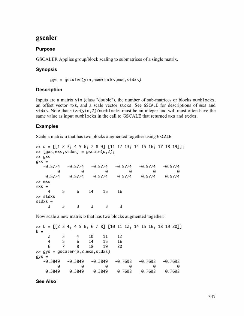
337

gscaler Purpose

GSCALER Applies group/block scaling to submatrices of a single matrix.

Synopsis gys = gscaler(yin,numblocks,mxs,stdxs)

Description

Inputs are a matrix yin (class "double"), the number of sub-matrices or blocks numblocks, an offset vector mxs, and a scale vector stdxs. See GSCALE for descriptions of mxs and stdxs. Note that size(yin,2)/numblocks must be an integer and will most often have the same value as input numblocks in the call to GSCALE that returned mxs and stdxs.

Examples

Scale a matrix a that has two blocks augmented together using GSCALE: >> a = [[1 2 3; 4 5 6; 7 8 9] [11 12 13; 14 15 16; 17 18 19]]; >> [gxs,mxs,stdxs] = gscale(a,2); >> gxs gxs = -0.5774 -0.5774 -0.5774 -0.5774 -0.5774 -0.5774 0 0 0 0 0 0 0.5774 0.5774 0.5774 0.5774 0.5774 0.5774 >> mxs mxs = 4 5 6 14 15 16 >> stdxs stdxs = 3 3 3 3 3 3

Now scale a new matrix b that has two blocks augmented together: >> b = [[2 3 4; 4 5 6; 6 7 8] [10 11 12; 14 15 16; 18 19 20]] b = 2 3 4 10 11 12 4 5 6 14 15 16 6 7 8 18 19 20 >> gys = gscaler(b,2,mxs,stdxs) gys = -0.3849 -0.3849 -0.3849 -0.7698 -0.7698 -0.7698 0 0 0 0 0 0 0.3849 0.3849 0.3849 0.7698 0.7698 0.7698

See Also

338

auto, gscale, mncn, mpca, scale, unfoldm

339

gselect Purpose

Selects subset of plotted line object points using a variety of interactive graphical modes.

Synopsis selected = gselect(mode,TargetHandle,modalwindow) [x,y] = gselect(mode,TargetHandle,modalwindow)

Description

GSELECT is a general utility which allows user-selection of plotted objects (points, line segments, areas of images, etc.). A variety of selection modes can be used on various types of plots. Each mode allows the user to select an area or range of the current axes. After selection is complete, the function returns a cell array that contains one cell for each line or image object on the axes. These cells contain a binary (true/false) array representing the selected points of each object.

The input mode is a string representing the selection mode. This governs how GSELECT selects objects in a figure. mode can be one of the following strings {default = 'rbbox'}: 'x': select a single x-axis position (snaps-to line x-data), 'y': select a single y-axis position (snaps-to line y-data), 'xs': select range of x-axis positions (snaps-to line x-data), 'ys': select range of y-axis positions (snaps-to line y-data), 'rbbox': select points inside a standard rubber-band box {default }, 'polygon': select points inside a polygon (user selects corners), 'paint': drag a broad line across points for selection, 'nearest': select single nearest point, 'all': selects all points (no user interaction required), and 'none': selects no points (no user interaction required).

Optional input TargetHandle is the handle or handles of objects to test for selection. The default is all lines, patches, surfaces, and images. The optional input modalwindow is a flag which, when set to 1, indicates that the figure should be made "modal" during selection (a modal window can not be inturrupted by other actions) {default = 0}.

The output is a cell array selection. Each cell in selection will be equal in length to the data used to create the corresponding object. For example, if a vector containing 30 points was plotted, the resulting cell will be a vector of 30 binary values. Each selected point on that object will be represented by a value of 1 (one) in the cell, unselected objects by a value of 0 (zero).

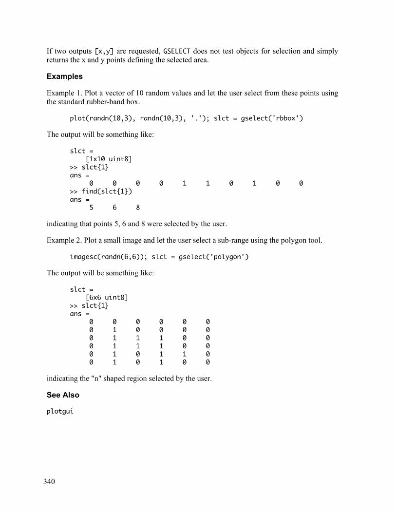
340

If two outputs [x,y] are requested, GSELECT does not test objects for selection and simply returns the x and y points defining the selected area.

Examples

Example 1. Plot a vector of 10 random values and let the user select from these points using the standard rubber-band box.

plot(randn(10,3), randn(10,3), '.'); slct = gselect('rbbox')

The output will be something like: slct = [1x10 uint8] >> slct{1} ans = 0 0 0 0 1 1 0 1 0 0 >> find(slct{1}) ans = 5 6 8

indicating that points 5, 6 and 8 were selected by the user.

Example 2. Plot a small image and let the user select a sub-range using the polygon tool. imagesc(randn(6,6)); slct = gselect('polygon')

The output will be something like: slct = [6x6 uint8] >> slct{1} ans = 0 0 0 0 0 0 0 1 0 0 0 0 0 1 1 1 0 0 0 1 1 1 0 0 0 1 0 1 1 0 0 1 0 1 0 0

indicating the "n" shaped region selected by the user.

See Also

plotgui

341

helppls Purpose

Starts the MATLAB help browser with PLS_Toolbox topics.

Synopsis helppls

Description

HELPPLS brings up the MATLAB help browser with a list of topics for installing and using the PLS_Toolbox. To access a particular topic simply click on its text.

Use the arrow buttons in the upper left corner of the window to navigate forward and backward (similar to a web browser). Some of the Topics may link you to a Documentation page about a particular function in the PLS_Toolbox. From here you can navigate to related topics by clicking on See Also items or to the next topic (in alphabetical order) by clicking its text in the yellow highlighted header/footer section.

See Also

readme

342

hline Purpose

Place a horizontal line in an existing figure.

Synopsis hline(y,lc) h = hline(y,lc)

Description

HLINE draws a horizontal line on an existing figure from the left axis to the right axis at a height, or heights, defined by y which can be a scalar or vector. If no input is used for y the default vaule is zero. The optional input variable lc can be used to define the line style and color as in normal plotting.

Examples

hline(1.4,'--b')

plots a horizontal dashed blue line at y = 1.4.

See Also

dp, ellps, plot, plttern, vline, zline

343

imagegui Purpose

Interface for Exploring Image PCA Scores.

Synopsis imagegui

Description

Models created by IMGPCA can be explored using IMAGEGUI. The function creates a set of linked score density plots along with a pseudocolor image based on the scores on the first 3 PCs. Users can select areas on any of the plots, and the pixels selected will be highlighted in the other plots.

IMAGEGUI can also be used to select data from the model as the original pixel indices of the data associated with selected areas can be saved to the workspace. Indices are saved as a cell array with each successive selection being the next cell in the array.

See Also

contrastmod, imread, imgselct, imgpca, imgsimca, isimcapr

344

imgpca Purpose

Principal Components Analysis of Multivariate Images.

Synopsis model = imgpca(mwa,scaling,nocomp) newmod = imgpca(mwa,model,plots)

Description

IMGPCA uses principal components analysis to make psuedocolor maps of multivariate images. The input is the multivariate image mwa.

Optional inputs are scaling the scaling to be used, scaling = 'auto', uses autoscaling {default}, scaling = 'mncn', uses mean centering, and caling = 'none', uses no scaling.

and the number of PCs to calculate nocomp.

It is assumed that the image (mwa) is a 3 dimensional (MxNxP) array where each image is MxN pixels and there are P images. IMGPCA presents each scores, residual, and T2 matrix as a psuedocolor image. If 3 are more PCs are selected (nocomp≥3), a composite of the first three PCs is shown as an rgb image, with red for the first PC, green for the second, and blue for the the third.

The output model is a structure with the following fields: xname: input data name, name: type of model, always 'IPCA', date: date of model creation, time: time of model creation, size: dimensions of input data, nocomp: number of PCs in model, scale: type of scaling used, means: mean vector for PCA model, stds: standard deviation vector for PCA model, ssq: variance captured table data, scores: PCA scores stored as MxNxnocomp array (uint8), range: original range of PCA scores before mapping to uint8, loads: PCA loadings, res: PCA residuals stored as m x n array (uint8),

345

reslim: Q limit, tsq: PCA T2 values stared as MxN array (unit8), and tsqlim: T2 limit.

Note that the scores, residuals and T2 matrices are stored as unsigned 8 bit integers (uint8) scaled so their range is 0 to 255. These can be viewed with the IMAGE function, but be sure the current colormap has 256 colors. For example, to view the scores on the second PC using the jet colormap: image(model.scores(:,:,2)), colormap(jet(256)), colorbar

See Also

contrastmod, imagegui, imread, imgselct, imgsimca, isimcapr

346

imgselct Purpose

Select an area on an image and return the pixel indices.

Synopsis [xinds,yinds] = imgselct

Description

When invoked, IMGSELCT allows the user to draw a polygon on an image using the mouse. To close the polygon a "return" is used. The x indices xinds and y indices yinds are returned.

See Also

contrastmod, imagegui, imread, imgpca, imgsimca, isimcapr

347

imgsimca Purpose

SIMCA Classification for Multivariate Images.

Synopsis model = imgsimca(img,data) newmod = imgsimca(data,model)

Description

This function allows the user to build SIMCA class models by outlining areas on a reference image img that correspond to areas on a multivariate image data. This image must be the same size (pixels by pixels) as the multivariate image data but can have a different depth (possibly due to having preprocessed the original data with IMGPCA).

The output is a structure array model which may be applied to new images with ISIMCAPR or IMGSIMCA. The fields of model are: imgname: name of original image variable, mwaname: name of original multivariate image data, name: model type, always 'IMGSIMCA', date: date stamp, time: time stamp, size: size of the image data, simcamod: simca model parameters (see SIMCA), in_class: array which gives pixels within 95% Q limits for each class, closest_class: array which gives closest class for each pixel, rqmat: reduced Q values for all classes for all pixels, and rtsqmat: reduced T2 values for all classes for all pixels.

Examples

To construct an image simca (IMGSIMCA) model model = imgsimca(img,data);

To make class predictions on a new multivariate image data use the model developed in IMGSIMCA and then call IMGSIMCA as newmod = imgsimca(data,model);

See Also

348

contrastmod, imagegui, imread, imgselct, imgpca, isimcapr

349

isimcapr Purpose

Applies IMGSIMCA models to new images.

Synopsis newmod = isimcapr(data,model)

Description

IMGSIMCA uses a model developed with the IMGSIMCA function model to classify areas on a new multivariate image data. Note that the new image can be of different size (i.e. it can have a different number of pixels than the original multivariate image used to construct the IMGSIMCA model (model)), but it must have the same depth.

The output is a structure array newmod which contains the new classifications. The fields of the structure are: mwaname: name of original multivariate image data, modelname: name of the original SIMCA model from IMGSIMCA, name: model type, always 'ISIMCAPR', date: date stamp, time: time stamp, size: size of the image data, in_class: array which gives pixels within 95% Q limits for each class, closest_class: array which gives closest class for each pixel, rqmat: reduced Q values for all classes for all pixels, and rtsqmat: reduced T2 values for all classes for all pixels.

See Also

contrastmod, imagegui, imread, imgselct, imgpca, imgsimca

350

jmlimit Purpose

Confidence limits for Q residuals via Jackson-Mudholkar.

Synopsis rescl = jmlimit(pc,s,cl)

Description

JMLIMIT estimates confidence limits for Q residuals based on the Jackson-Mudholkar method. See Jackson, J.E., “A User’s Guide to Principal Components”, John Wiley & Sons, New York, NY (1991), and the discussion in the Chemometrics Tutorial on PCA.

Inputs are the number of PCs used pc, the vector of eigenvalues s, and the confidence limit cl expressed as a fraction (e.g. 0.95). Note that for a PCA model structure, model, that the eigenvalues can be found in model.detail.ssq(:,2).

The output rescl is the confidence limit based on the method of Jackson and Mudholkar. See CHILIMIT for an alternate method of residual limit calculation based on chi squared.

Examples rescl = jmlimit(2,ssq(:,2),0.95);

For a PCA model contained in the structure model:

rescl = jmlimit(4,model.detail.ssq(:,2),0.99);

See Also

chilimit, analysis, pca, residuallimit

351

lamsel Purpose

Determine indices of wavelength axes in specified ranges.

Synopsis inds = lamsel(freqs,ranges,out)

Description

LAMSEL determines the indices of the elements of a wavelength or wavenumber axis within the ranges specified. Inputs are the wavelength or wavenumber axis freqs and an m by 2 matrix defining the wavelength ranges to select ranges.

An optional input out suppresses displaying information to the command window when set to 0.

The output inds is a vector of indices of channels in the specified range(s) inclusive.

Examples

inds = lamsel(lamda,[840 860; 1380 1400]);

outputs the indices of the elements of lamda between 840 and 860 and between 1380 and 1400.

See Also

baseline, savgol, specedit

352

lddlgpls Purpose

Provide an “load” dialog box for use with GUIs.

Synopsis [value,name,source] = lddlgpls(klass,message)

Description

LDDLPLS creates a dialog box that allows a function to load variables from the workspace or a MATLAB "mat" file into the function workspace. The location of the file to load from can be selecetd from the folders listed in the file list and from the "Look in" menu at the top of the dialog box. Optional input klass allows the user to select the workspace variable of class to load. Valid values for klass are: 'double': loads 2-way DOUBLE variable {default}, 'cell': loads CELL variable, 'char': loads 2-way CHAR variable, 'struct': loads a STRUCT variable, 'dataset': loads a DATASET object, 'doubdataset': loads a 2-way DOUBLE or DATASET, or '*': loads any class and size variable.

Optional text input message places a message in the load dialog box.

Outputs include value the value of the selected variable, name the original name of the variable, and location the filename from which the variable was loaded (will be empty if loaded from the base workspace).

See Also

erdlgpls, svdlgpls

353

leverag Purpose

Calculates sample leverage.

Synopsis lev = leverag(x,rinv)

Description

LEVERAG calculates the sample leverage according to

lev(i,1) = x(i,:)*inv(x'*x)*x(i,:)'.

Note that the leverage calculation should include a term for calculation of the offset (e.g. see Draper, N. and Smith, H., “Applied Regression Analysis, Second Edition”, John Wiley & Sons, New York, N.Y., 1981), but the above formula contains the salient information. This, in effect, assumes that the data have been mean centered and the constant term related to estimating the offset has been ignored. If x'*x is replaced by x'*x/(m-1) where m is the number of rows of x, and x has been mean centered then this is the equation for Hotelling's T2 statistic.

Note that if x is not of full rank then inv(x'*x) won't exist, or if x is nearly rank deficient then calculation of the inverse will be unstable. In these cases, the scores from principal components analysis can be used.

If the optional input rinv is supplied then the leverage is calculated as

lev(i,1) = x(i,:)*rinv*x(i,:)'.

See Also

doptimal, figmerit, pls, pcr

354

lsq2top Purpose

LSQ2TOP Fits a polynomial to the top/(bottom) of data.

Synopsis [b,resnorm,residual] = lsq2top(x,y,order,res,options)

Description

LSQ2TOP is an iterative least squares fitting algorithm. It is based on a weighted least squares approach where the weights are determined at each step. At initialization the weights are all 1, then a polynomial is fit through the data cloud using least squares. When fitting to the top of a data cloud, data points with a residual significantly below a defined limit (i.e. the points below the polynomial fit line) are given a small weighting. Therefore, on subsequent iterations these data points are weighted less in the fit, and the fit line moves to fit to the top of the data cloud.

Input x is the independent variable e.g. a Mx1 vector corresponding to a frequency or wavelength axis. Input y is the dependent variable e.g. a Mx1 vector corresponding to a measured spectrum. Input order is a scalar defining the order of polynomial to be fit e.g. y = P(x), and res is a scalar approximation of the fit residual e.g. noise level. Input options is discussed below. Note that the function can be used to fit to the top or bottom of a data cloud by changing trbflag in options.

The outputs are b, the regression coefficients [highest order term corresponds to b(1) and the intercept corresponds to b(end)], resnorm is the squared 2-norm of the residual, and residual is the fit residuals = y - P(x).

Options options = structure array with the following fields : display: [ 'off' | {'on'} ] governs level of display to command window. trbflag: [ 'top' | {'bottom'} ] top or bottom flag, tells algorithm to fit the

polynomials, y = P(x), to the top or bottom of the data cloud. tsqlim: [ 0.99 ] limit that governs whether a data point is significantly outside

the fit residual defined by input res. stopcrit: [1e-4 1e-4 1000 360] stopping criteria, iteration is continued until one

of the stopping criterion is met: [(relative tolerance) (absolute tolerance) (maximum number of iterations) (maximum time [seconds])].

355

Algorithm

For order = 1 and fitting to the top of a data cloud, LSQ2TOP finds the vector [ ]1 2b b=b

that minimizes ( ) ( )1 2 1 2Tb b b b− − − −y x 1 W y x 1 where W is a diagonal weighting matrix

whose elements are initially 1 and then are modified on each subsequent iteration.

The weighting is determined by first estimating the residuals for each data point j as 1 2j j jresidual b b= − −y x and defining /j jt residual res= where res is the input res. A

corresponding t-statistic from a t-table is estimated using the following tsqst = ttestp(1-options.tsqlim,5000,2);

where tablet is tsqst. The elements of W are then given by ( )1 0.5 /j j tablew t t= + for data

points with j tablet t< , and is a 1 otherwise. Therefore, the weighting is smaller for points far below the fit line.

The procedure can be modified to fit to the bottom of a data cloud by changing options.trbflag.

See Also

baseine, baselinew, fastnnls

356

lwrpred Purpose

Predictions based on locally weighted regression models.

Synopsis ypred = lwrpred(xnew,xold,yold,lvs,npts,out)

Description

LWRPRED makes new sample predictions ypred for a new matrix of independent variables xnew based on an existing data set of independent variables xold, and a vector of dependent variables yold. Predictions are made using a locally weighted regression model defined by the number principal components used to model the independent variables lvs and the number of points defined as local npts.

Optional input out suppresses printing of the results when set to 0 {default = 1}.

Note: Be sure to use the same scaling on new and old samples i.e. xnew must be scaled the same as xold!

See Also

lwrxy, pls, polypls

357

lwrxy Purpose

Predictions based on locally weighted regression with y-distance weighting.

Synopsis ypred = lwrxy(xnew,xold,yold,lvs,npts,alpha,iter,out)

Description

LWRXY makes new sample predictions ypred for a new matrix of independent variables xnew based on an existing data set of independent variables xold, and a vector of dependent variables yold. Predictions are made using a locally weighted regression model defined by the number principal components used to model the independent variables lvs, the number of points defined as local npts, the weighting given to the distance in y alpha, and the number of iterations to use iter.

Optional input out suppresses printing of the results when set to 0 {default = 1}.

Note: Be sure to use the same scaling on new and old samples i.e. xnew must be scaled the same as xold!

See Also

lwpred, pls, polypls

358

mcr Purpose

Multivariate curve resolution with constraints.

Synopsis [c,s] = mcr(x,c0,options) options = mcr('options')

Description

MCR decomposes a matrix X as CS such that X = CS + E where E is minimized in a least squares sense. Inputs are the matrix to be decomposed x (size m by n), and the initial guess c0. If c0 is size m by k, where k is the number of factors, then it is assumed to be the initial guess for C. If c0 is size k by n then it is assumed to be the initial guess for S. If m=n then, c0 is assumed to be the initial guess for C. Optional input options is described below.

The outputs are the estimated matrix c (m by k) and s (k by n). Usually c is a matrix of concentrations and s is a matrix of spectra. The function

[c,s] = mcr(x,c0)

will decompose x using an unconstrained alternating least squares calculation. This tends to lead to rotational ambiguities so it is common to include constraints. To include constraints use the options described below.

Note that if no non-zero equality constraints are imposed on a factor the spectra is normalized to unit length. This can lead to significant scaling differences between factors that have non-zero equality constraints and those that do not.

Options options = a structure array with the following fields: name: 'options', name indicating that this is an options structure, display: [ {'off'}| 'on' ], governs level of display to the command window, plots: [ 'none' | {'final'} ], governs level of plotting, ccon: [ 'none' | {'nonneg'} ], non-negativity on concentrations, scon: [ 'none' | {'nonneg'} ], non-negativity on spectra, cc: [ ], concentration equality constraints m by k matrix with NaN where

equality contraints are not applied and real value of the constraint where they are applied,

sc: [ ], spectra equality constraints k by n matrix with NaN where equality contraints are not applied and real value of the constraint where they are applied,

359

sclc: [ ], concentration scale axis vector with m elements otherwise 1:m is used (used in plotting),

scls: [ ], spectra scale axis vector with n elements otherwise 1:n is used (used in plotting),

tolc: [ {1e-5} ], tolerance on non-negativity for concentrations, tols: [ {1e-5} ], tolerance on non-negativity for spectra, ittol: [ {100} ], convergence criteria, if 0<ittol<1 then this is convergence tolerance {default = 1e-8}, and if ittol>=1 and integer, this is maximum number of iterations.

The default options can be retreived using: options = mcr('options');.

See Also

pca, parafac

360

mdcheck Purpose

Missing Data Checker and infiller.

Synopsis [flag,missmap,infilled] = mdcheck(data,options) options = mdcheck('options')

Description

This function checks for missing data and infills it using a PCA model if desired. The input is the data to be checked data. Optional input options is described below.

Outputs are the fraction of missing data flag, a map of the locations of the missing data as an unint8 variable missmap, and the data with the missing values filled in infilled.

Options options = a structure array with the following fields: name: 'options', name indicating that this is an options structure, options.frac_ssq: [{0.95}] desired fraction between 0 and 1 of variance to be

captured by the PCA model, options.max_pcs: [{5}] maximum number of PCs in the model, if 0, then it uses the

mean, options.meancenter: ['no' | {'yes'}], tells whether to use mean centering in the algorithm, options.display: [{'off'} | 'on'], governs level of display, options.tolerance: [{1e-6 100}] convergence criteria, the first element is the

minimum change and the second is the maximum number of iterations,

options.max_missing: [{0.4}] maximum fraction of missing data with which MDCHECK will operate, and

options.algorithm: [ {'svd'} | 'nipals' ] specified the missing data algorithm to use, NIPALS typically used for large amounts of missing data or large multi-way arrays.

Note: MDCHECK captures up to options.frac_ssq of the variance using options.max_pcs or fewer PCA components.

The default options can be retreived using: options = mdcheck('options');.

See Also

parafac, pca

361

medcn Purpose

Median center scales matrix to median zero.

Synopsis [mcx,mx,msg] = medcn(x,options)

Description

MEDCN centers a matrix x to it’s median and returns a matrix mcx with median zero columns and a vector of medians mx used to center the data. Optional input options is discussed below.

The output msg returns any warning messages.

Options options = a structure array with the following fields. display: [ {'off'} | 'on'] Governs screen display. matrix_threshold: {.15} Error threshold based on fraction of missing data in whole

matrix. column_threshold: {.25} Error threshold based on fraction of missing data in single

column.

See Also

auto, mncn, rescale, scale

362

mlpca Purpose

Maximum likelihood principal components analysis (user contributed).

Synopsis [U,S,V,SOBJ,ErrFlag] = mlpca(x,stdx,p)

Description

MLPCA performs maximum likelihood principal components analysis assuming uncorrelated measurement errors. This is a method that attempts to provide an optimal estimation of the p-dimensional subspace containing the data by taking into account uncertainties in the measurements, thereby dealing with those cases that cannot be treated by simple scaling. Inputs are x (m by n) the data matrix to be decomposed, stdx (m by n) matrix of standard deviations corresponding to the observations in x, and the number of factors into which the data is decomposed p. The outputs are U (m by p) orthonormal, S (p by p) diagonal, and V (n by p) orthonormal. The ML scores are given by U*S. Additional output SOBJ is the value of the objective function for the best model. For exact uncertainty estimates, this should follow a chi-squared distribution with (m-p)*(n-p) degrees of freedom. Additional output ErrFlag indicates the termination conditions of the function;

ErrFlag = 0: normal termination (convergence), or ErrFlag = 1: maximum number of iterations exceeded.

Also see:

P.D. Wentzell and M.T. Lohnes, “Maximum Likelihood Principal Component Analysis with Correlated Measurement Errors Theoretical and Practical Considerations”, Chemom. Intell. Lab. Syst., 45, 65-85 (1999).

P.D. Wentzell, D.T. Andrews, D.C. Hamilton, K. Faber, and B.R. Kowalski, "Maximum likelihood principal component analysis", J. Chemometrics 11(4), 339-366 (1997).

P.D. Wentzell, D.T. Andrews, and B.R. Kowalski, "Maximum likelihood multivariate calibration", Anal. Chem., 69, 2299-2311 (1997).

D.T. Andrews and P.D. Wentzell, "Applications of maximum likelihood principal components analysis: Incomplete data and calibration transfer", Anal. Chim. Acta, 350, 341-352 (1997).

See Also

analysis, mcr, parafac, pca

363

mncn Purpose

Mean center data matrices.

Synopsis [mcx,mx] = mncn(x,options)

Description

MNCN mean centers a matrix x and returns a matrix mcx with mean zero columns and a vector of means mx used to center the data.

See Also

auto, rescale, scale

364

modelstruct Purpose

Constructs an empty model structure.

Synopsis model = modelstruct(modeltype,pred)

Description

The output of many of the PLS_Toolbox functions is a single model structure in which the results of the analysis are contained. A structure is an organized group of variables all stored as "fields" of a single containing variable. The purpose of MODELSTRUCT is to create the empty model structures used by the various modeling routines. The type of structure requested is passed as the single string input modeltype and should be one of: 'pca', 'pcr', (for PCA or PCR models) 'nip', 'sim' (PLS models), or 'parafac' (PARAFAC model).

Once the structures created by MODELSTRUCT are filled-in by the appropriate function (e.g. PLS, PCR, PCA), they contain all the results of the analysis and can be used as a single object for making further predictions or plots from the modeling results. In many cases, these models can be passed whole to another function. For example:

opts.plots = 'none'; % turn off plots for PCA (see PCA) modl = pca(x, 3, opts); % create a PCA model from data X modlrder(modl); % display relevent model information plotscores(modl); % plot scores from model

Although the individual fields (contents) of each model vary between modeltypes, most contain at least these fields: modeltype: name of model, datasource: structure array with information about input data, date: date of creation, time: time of creation, info: additional model information, loads: cell array with model loadings for each mode/dimension, pred: cell array with model predictions for input data block (the first cell is

empty if options.blockdetail = 'normal'), tsqs: cell array with T2 values for each mode, ssqresiduals: cell array with sum of squares residuals for each mode, description: cell array with text description of model, and detail: sub-structure with additional model details and results.

365

Note that fields such as loads, tsqs and ssqresiduals are cell arrays of size [modes, blocks] where modes is the dimensionality of the data (e.g. for an array, modes = 2) and blocks is the number of blocks used by the analysis method (e.g. for PCA, blocks = 1, for PLS, blocks = 2). Thus, for a standard PCA model, loads will be a 2x1 cell containing "scores" in modl.loads{1,1} and traditional "loadings" in modl.loads{2,1}.

Because the models are standard MATLAB structures, they can be examined using standard structure notation:

>> modl.modeltype ans = PCA >> modl.loads ans = [30x4 double] [10x4 double]

Additionally, the individual components of a model can be "exploded" into individual variables using the EXPLODE function.

See Also

analysis, explode, parafac, pca, pcr, pls

366

modelviewer Purpose

Visualization of multi-way models.

Synopsis model = modelviewer(model,x);

Description

MODELVIEWER provides a graphical view of a model by enabling overview of scores, loadings, residuals etc. in one overall figure. Individual modes can be assessed by clicking plots and enlarged figures created by right-clicking plots.

INPUTS: model = PARAFAC, Tucker, or NPLS model, and x = X-block: predictor block (2-way array or DataSet Object).

OUTPUT: model = standard model structure (See MODELSTRUCT).

See Also

plotgui, plotloads, plotscores

367

modlpred Purpose

Predictions based on models created by ANALYSIS.

Synopsis [yprdn,resn,tsqn,scoresn] = modlpred(newx,modl,plots) [yprdn,resn,scoresn] = modlpred(newx,bin,p,q,w,lv,plots);

Description

MODLPRED makes Y-block predictions based on an X-block and an existing regression model created using ANALYSIS.

Inputs are the new X-block data newx in the units of the original data, the structure variable that contains the regression model modl, and an optional variable plots which suppresses the plots when set to 0 {default = 1}.

Outputs are the Y-block predictions yprdn, residuals resn, T2 values tsqn, and scores scoresn.

MODLPRED can also make predictions based on an existing PLS model constructed with the NIPALS algorithm from the PLS function. Inputs are the matrix of predictor variables newx, the PLS model inner-relation coefficients bin, the x-block loadings p, the y-block loadings q, the x-block weights w, the number of latent variables to use in prediction lv, and an optional variable plots which suppresses the plots when set to 0 {default = 1}.

Outputs are the Y-block predictions yprdn, residuals resn, and the scores scoresn. Note that T2 are not calculated.

See Also

analysis, explode, modlrder, pca, pcapro, pcr, pls

368

modlrder Purpose

Prints model information for standard model structures.

Synopsis modlrder(modl)

Description

MODLRDER reads information contained in a standard model structure variable modl and prints the information to the command window. It can be used with models created by the following functions: ANALYSIS, NPLS, PARAFAC, PCA, PCR, PLS, ANALYSIS.

Information includes date and time created and methods used to construct the model. There is no assignable output.

See Also

analysis, explode, modlpred, pcapro, ssqtable

369

mpca Purpose

Multi-way principal components analysis.

Synopsis model = mpca(mwa,ncomp,options) pred = mpca(mwa,model,options) options = mpca('options')

Description

Principal Components Analysis of multi-way data using unfolding to a 2-way matrix followed by conventional PCA.

Inputs to MPCA are the multi-way array mwa (class “double” or “dataset”) and the number of components to use in the model nocomp. To make predictions with new data the inputs are the multi-way array mwa and the MPCA model model. Optional input options is discussed below.

The output model is a structure array with the following fields: modeltype: 'MPCA', datasource: structure array with information about the x-block, date: date of creation, time: time of creation, info: additional model information, loads: 1 by 2 cell array with model loadings for each mode/dimension, pred: cell array with model predictions for each input data block (this is empty

if options.blockdetail = 'normal'), tsqs: cell array with T2 values for each mode, ssqresiduals: cell array with sum of squares residuals for each mode, description: cell array with text description of model, and detail: sub-structure with additional model details and results.

Options options = a structure array with the following fields. name: 'options', name indicating that this is an options structure, display: [ 'off' | {'on'} ] governs level of display to command window, plots: [ 'none' | {'final'} ] governs level of plotting, outputversion: [ 2 | {3} ] governs output format,

370

preprocessing: { [] } preprocessing structure, {default is mean centering i.e. options.preprocessing = preprocess('default', 'mean center')} (see PREPROCESS),

blockdetails: [ 'compact' | {'standard'} | 'all' ] extent of detail in predictions and residuals included in model structure ('standard' results in sum of squared residuals, and 'all' gives all x-block residuals), and

samplemode: [ {3} ] mode (dimension) to use as the sample mode e.g. if it is 3 then it is assumed that mode 3 is the sample/object dimension i.e. if mwa is 7x9x10 then the scores model.loads{1} will have 10 rows (it will be 10xncomp).

The default options can be retreived using: options = mpca('options');.

To use the defaults options and change the preprocessing, (options) can be input as a string with the following values: 'none': no scaling, 'auto': unfolds array then applies autoscaling, 'mncn': unfolds array then applies mean centering, or 'grps': {default} unfolds array then group/block scales each variable, i.e. the

same variance scaling is used for each variable along its time trajectory (see GSCALE).

MPCA will work with arrays of order 3 and higher. For higher order arrays, the last order is assumed to be the sample order, i.e. for an array of order n with the dimension of order n being m, the unfolded matrix will have m samples. For arrays of higher order the group scaling option will group together all data with the same order 2 index, for multiway array mwa, each mwa(:,j,:, ... ,:) will be scaled as a group.

See Also

gram, parafac, parafac2, pca, tld

371

mplot Purpose

Automatic creation of subplots and plotting.

Synopsis [rows,cols] = mplot(n,options) [rows,cols] = mplot([rows cols],options) [rows,cols] = mplot(y,options) [rows,cols] = mplot(x,y,options)

Description

Inputs can be one of three forms:

(1) the number of subplots requested n, “best fit” onto the figure

(2) the number of rows and columns for the subplot array [rows cols]

(3) or data to plot y with or without reference data for the x-axis x. Each column of y is plotted in a single subplot on the figure.

Outputs are the number of rows rows and columns cols used for the subplots.

Examples

Example 1. To automatically create a “best fit” of four empty subplots mplot(4)

Example 2. To automatically create four subplots in a 4 x 1 arrangement mplot([4 1])

Example 3. To automatically plot three random columns, each in its own subplot mplot(rand(100,3))

Options center: [ {'no'} | 'yes' ] governs centering of "left-over" plots at bottom of figure (when an uneven number of plots are to be fit onto the

screen, axismode : [ {''} | 'tight' ] governs axis settings

372

Algorithm

When mplot is doing the “best fit”, it attempts to keep the number of rows and columns as close as possible in size (Except for n=3 which is done as a 3x1 figure). Thus, the plot progression is: 1x1, 2x1, 3x1, 2x2, 3x2, 3x3, 4x3, etc.

See Also

plotgui, subplot

373

mscorr Purpose

Multiplicative scatter correction (MSC).

Synopsis [sx,alpha,beta,xref] = mscorr(x,xref,mc,win,specmode)

Description

MSCORR performs multiplicative scatter correction (a.k.a. multiplicative signal correction) on an input matrix of spectra x (class “double”) regressed against a reference spectra xref (class “double”).

If the optional input mc is 1 {default} then an intercept is used. If mc is set to 0 (zero) then a force fit through zero is used.

Optional input win is a NK element cell array of indices corresponding to windows to perform MSC, i.e. MSC is performed in each window win{i} for i=1:NK. In this case, (alpha and beta are not assigned).

Outputs are the corrected spectra sx, the intercepts/offsets alpha and the multiplicative scatter factor/slope beta.

Algorithm

For input spectra x (1xN) and reference spectra xref (1xN) the model is:

xTβ + α = xTref .

and the corrected spectra xs (1xN) is given by:

xs = (xref -α)/β .

See Also

stdfir, stdgen, frpcr

374

ncrossval Purpose

Cross-validation for multilinear PLS (NPLS).

Synopsis [press,cumpress,rmsecv,rmsec,cvpred,misclassed] = ncrossval(x,y,rm,cvi,ncomp,out,pre)

Description

Performs cross-validation of NPLS. If two-way unfold-PLS is desired convert input x to two-way x. By default, the data are centered across the first mode, but no scaling is applied. This can be changed by using additional input arguments.

INPUTS: x = X-block unfolded/matricized to two-way matrix, y = Y-block unfolded/matricized to two-way matrix, and rm = regression method (must be ‘npl’) cvi = see CROSSVAL ncomp = maximum number of factors. out = see CROSSVAL pre = see CROSSVAL

OUTPUT: See CROSSVAL

See Also

crossval, npls

375

nippls Purpose

NIPALS Partial Least Squares computational engine.

Synopsis [reg,ssq,xlds,ylds,wts,xscrs,yscrs,bin] = nippls(x,y,ncomp,options) options = nippls('options')

Description

Performs PLS regression using NIPALS algorithm.

INPUTS: x = X-block (M by Nx) and y = Y-block (M by Ny).

OPTIONAL INPUTS: nocomp = number of components {default = rank of X-block}, and options = discussed below.

The default options can be retreived using: options = nippls('options');.

OUTPUTS: reg = matrix of regression vectors, ssq = the sum of squares captured (ssq), xlds = X-block loadings, ylds = Y-block loadings, wts = X-block weights, xscrs = X-block scores, yscrs = Y-block scores, and bin = the inner relation coefficients.

Note: The regression matrices are ordered in reg such that each Ny (number of y variables) rows correspond to the regression matrix for that particular number of latent variables.

Options options = a structure containing the fields: name: 'options', name indicating that this is an options structure, and display: [ 'off' |{'on'}], governs display to command window.

See Also

376

pls, analysis, simpls

377

normaliz Purpose

Normalizes rows of matrix to unit vectors.

Synopsis [ndat,norms] = normaliz(dat) [ndat,norms] = normaliz(dat,out,normtype)

Description

NORMALIZ can be used for pattern normalization, which is useful for preprocessing in some pattern recognition applications.

The input is the data matrix dat. Optional input out suppresses warnings when set to 0 (zero) {default = 1} (warnings are given if the norm of a vector is zero). Optional input normtype can be used to specify the type of norm {default = 2}. If normtype is specified then out must be included, out can be empty [].

The output is the matrix of normalized data ndat where the rows have been normalized, and the vector of norms used in the normalization norms. Warnings are given for any vectors with zero norm.

Algorithm

For a 1 by N vector x, the norm nx is given by 1/

1

pN

px i

jn x

=

=

∑ where p is normtype. The

normalized 1 by N vector xn is given by x/nx.

See Also

auto, baseline, mncn, mscorr

378

npls Purpose

Multilinear-PLS (N-PLS) for true multi-way regression.

Synopsis model = npls(x,y,ncomp,options) pred = npls(x,ncomp,model,options) options = npls('options')

Description

NPLS fits a multilinear PLS1 or PLS2 regression model to x and y [R. Bro, J. Chemom., 1996, 10(1), 47-62]. The NPLS function also can be used for calibration and prediction.

INPUTS: x = X-block, y = Y-block, and ncomp = the number of factors to compute, or model = in prediction mode, this is a structure containing a NPLS model.

OPTIONAL INPUTS: options = discussed below.

OUTPUT: model = standard model structure (see: MODELSTRUCT) with the following fields: modeltype: 'NPLS', datasource: structure array with information about input data, date: date of creation, time: time of creation, info: additional model information, reg: cell array with regression coefficients, loads: cell array with model loadings for each mode/dimension, core: cell array with the NPLS core, pred: cell array with model predictions for each input data block, tsqs: cell array with T2 values for each mode, ssqresiduals: cell array with sum of squares residuals for each mode, description: cell array with text description of model, and detail: sub-structure with additional model details and results.

Options

379

options = options structure containing the fields: name: 'options', name indicating that this is an options structure, display: [ 'off' | {'on'} ], governs level of display to command window, plots: [ 'none' | {'final'} ], governs level of plotting, outputregrescoef: if this is set to 0 no regressions coefficients associated with the X-block

directly are calculated (relevant for large arrays), and blockdetails: [ {'standard'} | 'all' ], level of detail included in the model for

predictions and residuals.

See Also

datahat, explode, gram, mpca, outerm, parafac, pls, tld, unfoldm

380

npreprocess Purpose

Preprocessing of multi-way arrays.

Synopsis [prex,prepar] = npreprocess(x,prepar,undo,options) prex = npreprocess(x,setting) prex = npreprocess(x,prepar,1) options = npreprocess('options')

Description

NPREPROCESS is used for three different purposes:

1) for centering and scaling multi-way arrays in which case the parameters (offsets and scales) are first calculated and then applied to the data,

2) for preprocessing another data set according to (1), and

3) for transforming preprocessed data back (undo preprocessing).

INPUTS: x = data array, and settings = a two-row matrix (class "double") indicating which modes to center and

scale. The matrix is: settings = [cent; scal]. E.g. settings(1,:) = [1 0 1] => center across mode one and three, and settings(2,:) = [1 1 0] => scale to unit variance within mode one

and two.

OPTIONAL INPUTS: prepar = contains earlier defined mean and scale parameters, this data is required

for applying or undoing preprocessing, undo = when set to 1 this flag tells to undo/transform back, and options = discussed below.

OUTPUTS: prex = the preprocessed data, and prepar = a structure containing the necessary parameters to pre- and post-process

other arrays.

Options options = a structure array with the following fields:

381

name: 'options', identifies the structure as an options structure, display: [ {'on'} | 'off' ], governs level of display, iterproc: [ 'on' | {'off'} ], allows iterative preprocessing which is necessary

for some combinations of centering and scaling (see User Manual), scalefirst: [ {'on'} | 'off' ], defines that scaling is done before centering

which may have implications in complex combinations of preprocessing (see User Manual), and

usemse: [ {'on'} | 'off' ], defines that mean square scaling is used instead of scaling by standard deviations as is common in two-way analysis.

Examples

To apply preprocessing with options: [prex,prepar] = npreprocess(x,settings,[],0,options);

See Also

auto, mncn, preprocess, rescale, scale

382

oscapp Purpose

Applies orthogonal signal correction model to new data.

Synopsis newx = oscapp(x,nw,np,nofact)

Description

Inputs are the new data matrix x, weights from the OSC model nw, and loadings from the OSC np.

Optional input nofact can be used to restrict the correction to a smaller of factors than originally calculated.

The output is is the corrected data matrix newx.

Note: input data x must be centered and scaled like the original data!

See Also

crossval, osccalc

383

osccalc Purpose

Calculates orthogonal signal correction.

Synopsis [nx,nw,np,nt] = osccalc(x,y,nocomp,iter,tol)

Description

Inputs are the matrix of scaled predictor variables x, scaled predicted variable(s) y, and the number of OSC components nocomp.

Optional inputs are the maximum number of iterations used in attempting to maximize the variance captured by othogonal components iter {default = 0}, and the tolerance on percent of x variance to consider when forming the final w vector tol {default = 99.9}.

Outputs are the OSC corrected predictor matrix nx, and the x-block weigths nw, loads np, and scores nt that were used in making the correction.

Once the calibration is done, new (scaled) X data can be corrected by newx = x - x*nw*inv(np'*nw)*np';. See OSCAPP.

See Also

crossval, oscapp

384

outerm Purpose

Computes the outer product of any number of vectors with multiple factors.

Synopsis mwa = outerm(facts,lo,vect)

Description

The input to outer is a 1 by N cell array facts, where each cell contains a matrix of factors for one of the modes (a.k.a. ways, dimensions, or orders), with each factor being a column in the matrix.

Optional inputs are lo the number of a mode to leave out in the formation of the outer product, and a flag vect which causes the function to not sum and reshape the final factors when set to 1. (This option is used in the alternating least squares steps in PARAFAC.)

The output is the multiway array resulting from multiplying the factors together mwa, or the strung out individual factors.

Examples: a = [[1:7]' [2 4 1 3 5 7 6]']; % 7x2 b = [sin([1:.5:5]') cos([1:.5:5]')]; % 9x2 c = [[1:8 0 0]', [0 0 1:8]']; % 10x2 x = outerm({a,b,c}); % 7x9x10

See Also

gram, mpca, parafac, tld

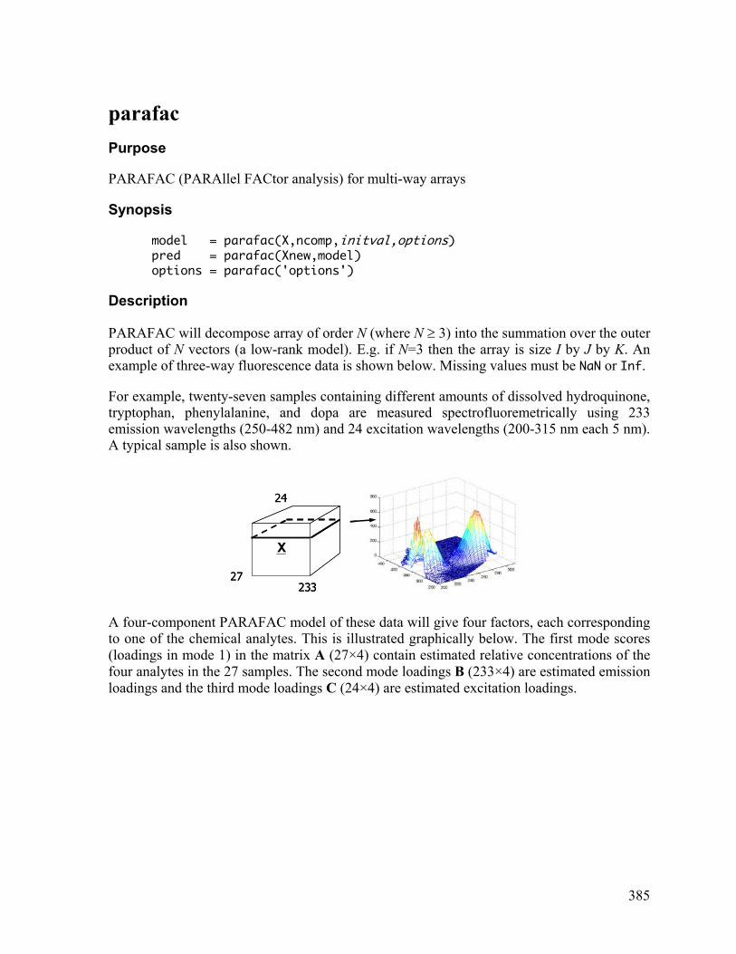
385

parafac Purpose

PARAFAC (PARAllel FACtor analysis) for multi-way arrays

Synopsis model = parafac(X,ncomp,initval,options) pred = parafac(Xnew,model) options = parafac('options')

Description

PARAFAC will decompose array of order N (where N ≥ 3) into the summation over the outer product of N vectors (a low-rank model). E.g. if N=3 then the array is size I by J by K. An example of three-way fluorescence data is shown below. Missing values must be NaN or Inf.

For example, twenty-seven samples containing different amounts of dissolved hydroquinone, tryptophan, phenylalanine, and dopa are measured spectrofluoremetrically using 233 emission wavelengths (250-482 nm) and 24 excitation wavelengths (200-315 nm each 5 nm). A typical sample is also shown.

X

27

24

233

X

27

24

233

A four-component PARAFAC model of these data will give four factors, each corresponding to one of the chemical analytes. This is illustrated graphically below. The first mode scores (loadings in mode 1) in the matrix A (27×4) contain estimated relative concentrations of the four analytes in the 27 samples. The second mode loadings B (233×4) are estimated emission loadings and the third mode loadings C (24×4) are estimated excitation loadings.

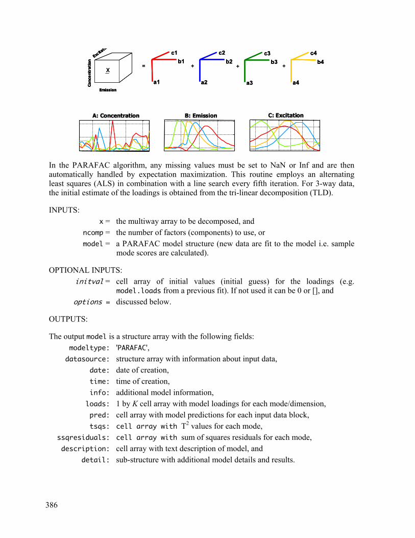
386

A: Concentration B: Emission C: Excitation

X= +

c2b2

a2

c1b1

a1

+

c3b3

a3

+

c4b4

a4Conc

ent

rati

onEmission

Excita

tio

A: Concentration B: Emission C: Excitation

X= +

c2b2

a2

c1b1

a1

+

c3b3

a3

+

c4b4

a4Conc

ent

rati

onEmission

Excita

tio

X= +

c2b2

a2

c1b1

a1

+

c3b3

a3

+

c4b4

a4Conc

ent

rati

onEmission

Excita

tio

In the PARAFAC algorithm, any missing values must be set to NaN or Inf and are then automatically handled by expectation maximization. This routine employs an alternating least squares (ALS) in combination with a line search every fifth iteration. For 3-way data, the initial estimate of the loadings is obtained from the tri-linear decomposition (TLD).

INPUTS: x = the multiway array to be decomposed, and ncomp = the number of factors (components) to use, or model = a PARAFAC model structure (new data are fit to the model i.e. sample

mode scores are calculated).

OPTIONAL INPUTS: initval = cell array of initial values (initial guess) for the loadings (e.g.

model.loads from a previous fit). If not used it can be 0 or [], and options = discussed below.

OUTPUTS:

The output model is a structure array with the following fields: modeltype: 'PARAFAC', datasource: structure array with information about input data, date: date of creation, time: time of creation, info: additional model information, loads: 1 by K cell array with model loadings for each mode/dimension, pred: cell array with model predictions for each input data block, tsqs: cell array with T2 values for each mode, ssqresiduals: cell array with sum of squares residuals for each mode, description: cell array with text description of model, and detail: sub-structure with additional model details and results.

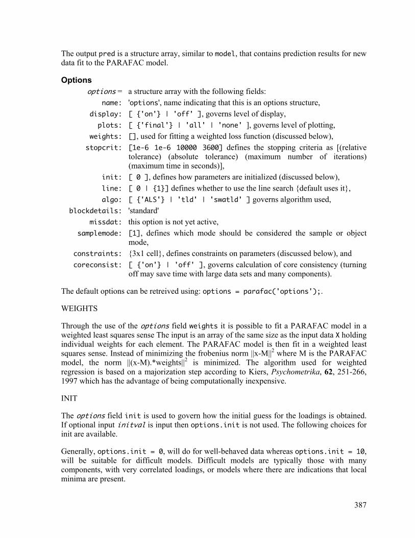
387

The output pred is a structure array, similar to model, that contains prediction results for new data fit to the PARAFAC model.

Options options = a structure array with the following fields: name: 'options', name indicating that this is an options structure, display: [ {'on'} | 'off' ], governs level of display, plots: [ {'final'} | 'all' | 'none' ], governs level of plotting, weights: [], used for fitting a weighted loss function (discussed below), stopcrit: [1e-6 1e-6 10000 3600] defines the stopping criteria as [(relative

tolerance) (absolute tolerance) (maximum number of iterations) (maximum time in seconds)],

init: [ 0 ], defines how parameters are initialized (discussed below), line: [ 0 | {1}] defines whether to use the line search {default uses it}, algo: [ {'ALS'} | 'tld' | 'swatld' ] governs algorithm used, blockdetails: 'standard' missdat: this option is not yet active, samplemode: [1], defines which mode should be considered the sample or object

mode, constraints: {3x1 cell}, defines constraints on parameters (discussed below), and coreconsist: [ {'on'} | 'off' ], governs calculation of core consistency (turning

off may save time with large data sets and many components).

The default options can be retreived using: options = parafac('options');.

WEIGHTS

Through the use of the options field weights it is possible to fit a PARAFAC model in a weighted least squares sense The input is an array of the same size as the input data X holding individual weights for each element. The PARAFAC model is then fit in a weighted least squares sense. Instead of minimizing the frobenius norm ||x-M||2 where M is the PARAFAC model, the norm ||(x-M).*weights||2 is minimized. The algorithm used for weighted regression is based on a majorization step according to Kiers, Psychometrika, 62, 251-266, 1997 which has the advantage of being computationally inexpensive.

INIT

The options field init is used to govern how the initial guess for the loadings is obtained. If optional input initval is input then options.init is not used. The following choices for init are available.

Generally, options.init = 0, will do for well-behaved data whereas options.init = 10, will be suitable for difficult models. Difficult models are typically those with many components, with very correlated loadings, or models where there are indications that local minima are present.

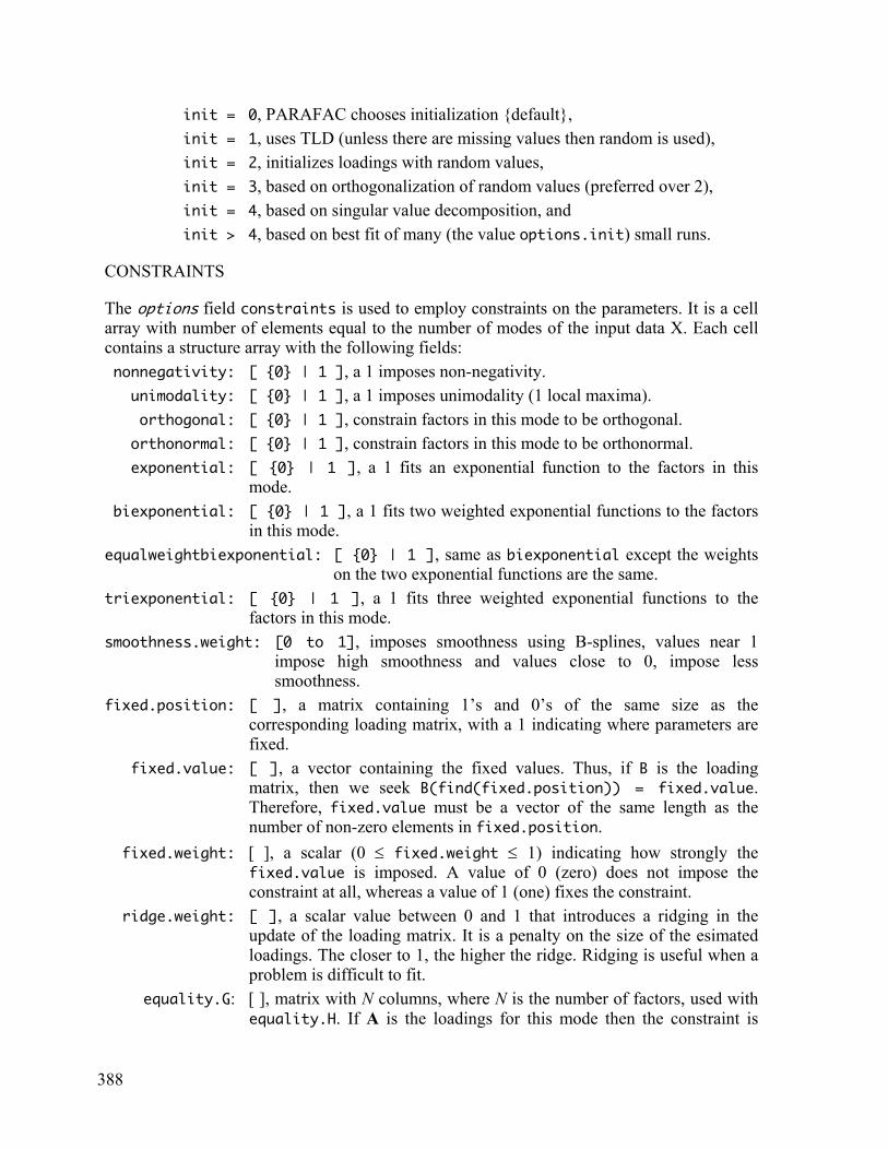
388

init = 0, PARAFAC chooses initialization {default}, init = 1, uses TLD (unless there are missing values then random is used), init = 2, initializes loadings with random values, init = 3, based on orthogonalization of random values (preferred over 2), init = 4, based on singular value decomposition, and init > 4, based on best fit of many (the value options.init) small runs.

CONSTRAINTS

The options field constraints is used to employ constraints on the parameters. It is a cell array with number of elements equal to the number of modes of the input data X. Each cell contains a structure array with the following fields: nonnegativity: [ {0} | 1 ], a 1 imposes non-negativity. unimodality: [ {0} | 1 ], a 1 imposes unimodality (1 local maxima). orthogonal: [ {0} | 1 ], constrain factors in this mode to be orthogonal. orthonormal: [ {0} | 1 ], constrain factors in this mode to be orthonormal. exponential: [ {0} | 1 ], a 1 fits an exponential function to the factors in this

mode. biexponential: [ {0} | 1 ], a 1 fits two weighted exponential functions to the factors

in this mode. equalweightbiexponential: [ {0} | 1 ], same as biexponential except the weights

on the two exponential functions are the same. triexponential: [ {0} | 1 ], a 1 fits three weighted exponential functions to the

factors in this mode. smoothness.weight: [0 to 1], imposes smoothness using B-splines, values near 1

impose high smoothness and values close to 0, impose less smoothness.

fixed.position: [ ], a matrix containing 1’s and 0’s of the same size as the corresponding loading matrix, with a 1 indicating where parameters are fixed.

fixed.value: [ ], a vector containing the fixed values. Thus, if B is the loading matrix, then we seek B(find(fixed.position)) = fixed.value. Therefore, fixed.value must be a vector of the same length as the number of non-zero elements in fixed.position.

fixed.weight: [ ], a scalar (0 ≤ fixed.weight ≤ 1) indicating how strongly the fixed.value is imposed. A value of 0 (zero) does not impose the constraint at all, whereas a value of 1 (one) fixes the constraint.

ridge.weight: [ ], a scalar value between 0 and 1 that introduces a ridging in the update of the loading matrix. It is a penalty on the size of the esimated loadings. The closer to 1, the higher the ridge. Ridging is useful when a problem is difficult to fit.

equality.G: [ ], matrix with N columns, where N is the number of factors, used with equality.H. If A is the loadings for this mode then the constraint is

389

imposed such that GAT = H. For example, if G is a row vector of ones and H is a vector of ones (1’s), this would impose closure.

equality.H: [ ], matrix of size consistent with the constriant imposed by equality.G.

equality.weight: [ ], a scalar (0 ≤ equality.weight ≤ 1) indicating how strongly the equality.H and equality.G is imposed. A value of 0 (zero) does not impose the constraint at all, whereas a value of 1 (one) fixes the constraint.

leftprod: [0], If the loading matrix, B is of size JxR, the leftprod is a matrx G of size JxM. The loading B is then constrained to be of the form B = GH, where only H is updated. For example, G may be a certain JxJ subspace, if the loadings are to be within a certain subspace.

rightprod: [0], If the loading matrix, B is of size JxR, the rightprod is a matrx G of size MxR. The loading B is then constrained to be of the form B = HG, where only H is updated. For example, if rightprod is [1 1 0;0 0 1], then the first two components in B are forced to be the same.

iterate_to_conv: [0], Usually the constraints are imposed within an iterative algorithm. Some of the constraints use iterative algorithms themselves. Setting iterate_to_conv to one, will force the iterative constraint algorithms to continue until convergence.

timeaxis: [], This field (if supplied) is used as the time axis when fitting loadings to a function (e.g. see exponential). Therefore, it must have the same number of elements as one of the loading vectors for this mode.

description: [1x1592 char],

If the constraint in a mode is set as fixed, then the loadings of that mode will not be updated, hence the initial loadings stay fixed.

Examples

parafac demo gives a demonstration of the use of the PARAFAC algorithm.

model = parafac(X,5) fits a five-component PARAFAC model to the array X using default settings.

pred = parafac(Z,model) fits a parafac model to new data Z. The scores will be taken to be in the first mode, but you can change this by setting options.samplemodex to the mode which is the sample mode. Note, that the sample-mode dimension may be different for the old model and the new data, but all other dimensions must be the same.

options = parafac('options'); generates a set of default settings for PARAFAC. options.plots = 0; sets the plotting off.

options.init = 3; sets the initialization of PARAFAC to orthogonalized random numbers.

options.samplemodex = 2; Defines the second mode to be the sample-mode. Useful, for example, when fitting an existing model to new data.

390

model = parafac(X,2,[],options); fits a two-component PARAFAC model with the settings defined in options.

parafac io shows the I/O of the algorithm.

parafac '<string>' shows the extended help on selected subjects in <string>. Possible string values: 'initval', 'options', 'constraints', 'weights', 'init'.

See Also

datahat, explode, gram, mpca, outerm, parafac2, tld, tucker, unfoldm

391

parafac2 Purpose

PARAFAC2 (PARAllel FACtor analysis2) for multi-way arrays

Synopsis model = parafac2(X,ncomp); %decomposition model = parafac2(X,ncomp,initval); model = parafac2(X,ncomp,initval,options); pred = parafac2(Xnew,model); %application options = parafac2('options');

Description

The three-way PARAFAC2 model is best perceived as a model close to the ordinary PARAFAC model. The major difference is that strict trilinearity is no longer required, so PARAFAC2 can sometimes handle elution time shifts, varying batch trajectories etc. The ordinary PARAFAC model is also sometimes called the PARAFAC1 model to distinguish it from the PARAFAC2 model.

In the PARAFAC1 model, one loading matrix is found for each mode. That implies that this loading matrix is the same across all levels for the other modes. For example, in a PARAFAC1 model of a data set with chromatographic spectrally detected experiments, the PARAFAC1 model ideally provides a loading matrix for e.g. the chromatographic mode which holds the true elution profiles of the chemical analytes. Thus, the PARAFAC1 model assumes that these elution profiles do not change shape in different experiments (only their magnitude). Such an assumption may be too strict and invalid. A little model error is seldom problematic, but if the structure of the data deviates considerably from the assumptions of the model, it can be impossible to fit a reasonable model. In the PARAFAC2 model, this trilinearity assumption is relaxed in one mode. A PARAFAC1 model of a three-way array is given by A, B and C (loading matrices in first, second and third mode). In PARAFAC2, the loadings in one mode can change from level to level. That is, assume that the third mode (C) of dimension K holds different samples (it is common practice, to have samples in the last mode for PARAFAC2). Instead of having a fixed first mode loading A for all samples, A may now vary from sample to sample. Thus for each sample, k, there is an individual A called Ak. The only restriction on Ak is that the cross-product Ak

TAk remains constant. This is in contrast to PARAFAC1 where A is simply the same for all k.

Another way of imposing this constraint (AkTAk constant) is to say that each Ak is modeled

as PkH where Pk is an orthogonal matrix of the same size as Ak and where H is a small quadratic matrix with dimension equal to the number of components. This different interpretation of the concept shows that the individual components Ak only differ up to a rotation. Hence, the latent variables are the same for all samples but may manifest themselves through different rotations.

392

The situations in which the PARAFAC2 model is valid can be difficult to understand because the flexibility compared to the PARAFAC1 model is somewhat abstract. However, one simple way to see the applicability of the PARAFAC2 model is that PARAFAC2 is worth considering in situations in which PARAFAC1 should ideally be valid, but where practical applications show that it is not. For example, it is often observed that the differences in elution profiles from experiment to experiment in chromatography makes the PARAFAC1 model difficult to fit. Many times PARAFAC2 can still handle such deviations even when the shifts in retention times are quite severe.

It is possible to fit both the PARAFAC1 and the PARAFAC2 model. If both models give the same results (approximately), then PARAFAC1 is likely valid and then PARAFAC1 is preferred because it uses fewer degrees of freedom. If there are large deviations, PARAFAC2 may be preferred. Note, though, that the K matrices Ak may have a larger variability than the corresponding A from the PARAFAC1 model because of the smaller amount of data that it is estimated from. This does not imply inadequacy but simply that there are differences in the way that the parameters are estimated.

Another interesting type of application of PARAFAC2 follows from the insight that the constraint that Ak

TAk is constant. This directly implies that the individual slabs, Xk, of the array can have different lengths, hence different size Ak, yet still fulfill the constraint that Ak

TAk is constant. Thus, PARAFAC2 can also handle e.g. batch data where the data from each batch are obtained at different sampling rates or different sampling duration. This is a very powerful feature of the PARAFAC2 model compared to the PARAFAC1 model.

The three-way PARAFAC2 model is given

Xk = AkDkBT + Ek = PkHDkBT + Ek, k = 1, .., K

Xk is a slab of data (I×J) in which I may actually vary with K. K is the number of slabs and Ak (I×ncomp) are the first-mode loadings for the kth sample. Dk is a diagonal matrix that holds the kth row of C in its diagonal. C (K×comp) is the third mode loadings, H is an (ncomp×ncomp) matrix, and Pk is an (I×ncomp) orthogonal matrix. The output P is given as a cell array of length K where the kth cell element holds the (I×ncomp) matrix Pk. Thus, to get e.g. the second sample P, write P{2}, and to get the estimate of the first mode loadings, Ak, at this second frontal slab (k = 2), write P{2}*H.

The model can also be fitted to more than three-way data. It is important then to be aware which mode is supposed to be fitted by separate loadings for each sample. The convention is that the first mode is the mode that has individual loadings and that these are defined across the last (the sample) mode. For example, chromatographic data with spectral detection can be arranged as the first mode being elution, the second spectral and the third mode being different experiments. Then different elution profiles (mode one) are found for each experiment (mode three). For multivariate batch process data, the array is typically arranged as time × variables × batches, meaning that the time trajectories (mode one) can vary from batch to batch (mode three).

INPUTS: x = the multiway array to be decomposed,

393

If all slabs have similar size, x is an array. For example, for three-way data where the matrix of measurements for sample one is held in x1, for sample 2 in x2 etc. then X(:,:,1) = X1; X(:,:,2) = X2; etc. If the slabs have different size, X is a cell array (type <help cell> for more info on cells). Then X{1} = X1; X{2} = X2; etc., and

ncomp = the number of factors (components) to use, or model = a PARAFAC model structure (new data are fit to the model i.e. sample

mode scores are calculated).

OPTIONAL INPUTS: initval = cell array of initial values (initial guess) for the loadings (e.g.

model.loads from a previous fit). If not used it can be 0 or [], and options = discussed below.

OUTPUTS:

Data that are input as a cell-array in PARAFAC2 are converted to an array by zero-padding each samples first mode dimension in case of different first mode dimensions for different samples. Residuals etc. are also output as arrays. The output model is a structure array with the following fields: modeltype: 'PARAFAC2', datasource: structure array with information about input data, date: date of creation, time: time of creation, info: additional model information, loads: 1 by K cell array with model loadings for each mode/dimension, pred: cell array with model predictions for each input data block, tsqs: cell array with T2 values for each mode, ssqresiduals: cell array with sum of squares residuals for each mode, description: cell array with text description of model, and detail: sub-structure with additional model details and results. The output pred is a structure array, similar to model, that contains prediction results for new data fit to the PARAFAC model.

Options options = a structure array with the following fields: name: 'options', name indicating that this is an options structure, display: [ {'on'} | 'off' ], governs level of display, plots: [ {'final'} | 'all' | 'none' ], governs level of plotting, weights: [], used for fitting a weighted loss function (discussed below),

394

stopcrit: [1e-6 1e-6 10000 3600] defines the stopping criteria as [(relative tolerance) (absolute tolerance) (maximum number of iterations) (maximum time in seconds)],

init: [ 0 ], defines how parameters are initialized (discussed below), line: [ 0 | {1}] defines whether to use the line search {default uses it}, algo: [ {'ALS'} | 'tld' | 'swatld' ] governs algorithm used, blockdetails: 'standard' missdat: this option is not yet active, samplemode: [3], defines which mode should be considered the sample or object

mode, constraints: {3x1 cell}, defines constraints on parameters (see PARAFAC), and coreconsist: [ {'on'} | 'off' ], governs calculation of core consistency (turning

off may save time with large data sets and many components).

The default options can be retreived using: options = parafac('options');.

Note that samplemode should not be altered in PARAFAC2.

WEIGHTS

See help on PARAFAC for help on the use of weights for PARAFAC2

CONSTRAINTS

See help on PARAFAC for help on the use of constraints for PARAFAC2. One important difference from PARAFAC is that constraints in the first mode do not apply to the estimated profiles, Ak, themselves but only to H. It is generally adviced not to use constraints in the first mode.

Examples parafac2 demo for a demonstration of the use of the PARAFAC2 algorithm. model = parafac2(X,5) fits a five-component PARAFAC2 model to the array X using default settings. options = parafac2('options'); generates a set of default settings for PARAFAC2. options.plots = 0; sets the plotting off. options.init = 3; sets the initialization of PARAFAC2 to orthogonalized random numbers. model = parafac2(X,2,options); fits a two-component PARAFAC2 model with the settings defined in options. parafac2 io shows the I/O of the algorithm.

395

See Also

datahat, explode, gram, mpca, outerm, parafac, tld, tucker, unfoldm

396

pca Purpose

Perform principal components analysis.

Synopsis pca model = pca(data,ncomp,options); %decomposition pred = pca(newdata,model,options); %application options = pca('options')

Description

Performs a principal component analysis decomposition of the input array data returning ncomp principal components. E.g. for an M by N matrix X the PCA model is X = TPT + E, where the scores matrix T is M by K, the loadings matrix P is N by K, the residuals matrix E is M by N, and K is the number of factors or principal components ncomp. The output model is a PCA model structure. This model can be applied to new data by passing the model structure to PCA along with new data newdata or by using PCAPRO. The output of PCA is a model structure with the following fields (see MODELSTRUCT for additional information): modeltype: 'PCA', datasource: structure array with information about input data, date: date of creation, time: time of creation, info: additional model information, loads: cell array with model loadings for each mode/dimension, pred: cell array with model predictions for the input block (when

blockdetail='normal' x-block predictions are not saved and this will be an empty array)

tsqs: cell array with T2 values for each mode, ssqresiduals: cell array with sum of squares residuals for each mode, description: cell array with text description of model, and detail: sub-structure with additional model details and results.

If the inputs are a Mnew by N matrix newdata and and a PCA model model, then PCA applies the model to the new data. Preprocessing included in model will be applied to newdata. The output pred is structure, similar to model, that contains the new scores, and other predictions for newdata.

Note: Calling pca with no inputs starts the graphical user interface (GUI) for this analysis method.

Options

397

options = a structure array with the following fields: name: 'options', name indicating that this is an options structure, display: [ 'off' | {'on'} ], governs level of display to command window, plots: [ 'none' | {'final'} ], governs level of plotting. outputversion: [ 2 | {3} ], governs output format (discussed below), preprocessing: {[]}, cell array containing a preprocessing structure (see PREPROCESS)

defining preprocessing to use on the data (discussed below), blockdetails: [ {'standard'} | 'all' ], level of detail included in the model for

predictions and residuals.

The default options can be retreived using: options = pca('options');.

OUTPUTVERSION

By default (options.outputversion = 3) the output of the function is a standard model structure model. If options.outputversion = 2, the output format is:

[scores,loads,ssq,res,reslm,tsqlm,tsq] = pca(xblock1,2,options);

where the outputs are scores = x-block scores, loads = x-block loadings ssq = the sum of squares information, res = the Q residuals, reslim = the estimated 95% limit line for Q residuals, tsqlim = the estimated 95% limit line for T2, and tsq = the Hotelling’s T2 values.

PREPROCESSING

The preprocessing field can be empty [] (indicating that no preprocessing of the data should be used), or it can contain a preprocessing structure output from the PREPROCESS function. For example options.preprocessing = {preprocess('default', 'autoscale')}. This information is echoed in the output model in the model.detail.preprocessing field and is used when applying the PCA model to new data.

See Also

analysis, evolvfa, ewfa, explode, parafac, plotloads, plotscores, preprocess, ssqtable

398

pcaengine Purpose

Principal components analysis computational engine.

Synopsis [ssq,datarank,loads,scores,msg] = pcaengine(data,ncomp,options) options = pcaengine('options')

Description

This function is intended primarily for use as the engine behind other more full featured PCA programs. The only required input is the data matrix data.

Optional inputs include the number of principal components desired in the output ncomp, and a structure containing optional inputs options. If the number of components ncomp is not specified, the routine will return components up to the rank of the data datarank.

The outputs are the variance or sum-of-squares captured table ssq, mathematical rank of the data datarank, principal component loadings loads, principal component scores scores, and a text variable containing any warning messages msg.

To enhance speed, the routine is written so that only the specified outputs are computed.

Options options = a structure array with the following fields: name: 'options', name indicating that this is an options structure, display: [ 'off' | {'on'} ], governs level of display to command window, algorithm: [ {'regular'} | 'big' | 'auto'], tells which algorithm to use, 'regular', uses an SVD and calculates all eigenvectors and

eigenvalues, 'big', calculates the “economy size” SVD, and 'auto', checks the size of the data matrix and automatically chooses

between 'regular' and 'big'

The default options can be retreived using: options = pcaengine('options');.

See Also

analysis, evolvfa, ewfa, explode, parafac, pca, ssqtable

399

pcapro Purpose

Project new data onto an existing principal components model.

Synopsis [scoresn,resn,tsqn] = pcapro(newdata,loads,ssq,reslm,tsqlm,plots) [scoresn,resn,tsqn] = pcapro(newdata,pcamod,plots)

Description

Inputs can be in two forms: 1) as a list of input variables, or 2) as a single model structure variable returned by ANALYSIS or PCA.

1) If a list of input variables is used the inputs are the new data newdata scaled the same as the original data used to construct the model, the model loadings loads, the model variance info ssq, the limit for Q reslm, the limit for T2 tsqlm, and an optional variable plots which suppresses plotting when set to 0 {default plots = 1}.

WARNING: Scaling for newdata should be the same as original data used to create the PCA model!

The I/O format is: [scoresn,resn,tsqn] = pcapro(newdata,loads,ssq,q,tsq,plots)

2) If the PCA model is input as the single model structure variable returned by ANALYSIS or PCA then the inputs are the new data newdata in the units of the original data, the structure variable that contains the PCA model pcamod, and an optional variable plots which suppresses the plots when set to 0 {default plots = 1}.

NOTE: newdata will be preprocessed in PCAPRO using information stored in pcamod (pcamod.detail.preprocessing).

The I/O format is: [scoresn,resn,tsqn] = pcapro(newdata,pcamod,plots)

Outputs are the new scores scoresn, residuals resn, and T2 values tsqn. These are plotted if plots = 1 {default}.

See Also

datahat, analysis, explode, modlpred, pca, simca, tsqmtx

400

pcolormap Purpose

Produces a pseudocolor map with labels.

Synopsis pcolormap(data,maxdat,mindat) pcolormap(data,xlbl,ylbl,maxdat,mindat)

Description

PCOLORMAP produces a pseudocolor map of the M by N input matrix data.

If data is class “double” the I/O format is: pcolormap(data,xlbl,ylbl,maxdat,mindat)

If data is class “dataset” the I/O format is: pcolormap(data,maxdat,mindat)

Optional inputs are xlbl a character array with M rows of labels for mode 1 {default = int2str([1:m]')}, ylbl a character array with N rows of labels for mode 2 {default = int2str([1:n]')}, maxdat a user defined maximum {default = max(max(data)')}, and mindat a user defined minimum {default = min(min(data)')}.

See Also

corrmap, pcolor, rwb

401

pcr Purpose

Principal components regression: multivariate inverse least squares regession.

Synopsis model = pcr(x,y,ncomp,options) %calibration pred = pcr(x,model,options) %prediction valid = pcr(x,y,model,options) %validation options = pcr('options')

Description

PCR calculates a single principal components regression model using the given number of components ncomp to predict y from measurements x.

To construct a PCR model, the inputs are x the predictor x-block (2-way array class “double” or “dataset”), y the predicted y-block (2-way array class “double” or “dataset”), ncomp the number of components to to be calculated (positive integer scalar) and the optional structure, options. The output is a standard model structure model with the following fields (see MODELSTRUCT): modeltype: 'PCR', datasource: structure array with information about input data, date: date of creation, time: time of creation, info: additional model information, reg: regression vector, loads: cell array with model loadings for each mode/dimension, pred: 2 element cell array with model predictions for each input block (when

options.blockdetail='normal' x-block predictions are not saved and this will be an empty array) and the y-block predictions.

tsqs: cell array with T2 values for each mode, ssqresiduals: cell array with sum of squares residuals for each mode, description: cell array with text description of model, and detail: sub-structure with additional model details and results.

To make predictions the inputs are x the new predictor x-block (2-way array class “double” or “dataset”), and model the PCR model. The output pred is a structure, similar to model, that contains scores, predictions, etc. for the new data.

If new y-block measurements are also available then the inputs are x the new predictor x-block (2-way array class “double” or “dataset”), y the new predicted block (2-way array class “double” or “dataset”), and model the PCR model. The output valid is a structure, similar to

402

model, that contains scores, predictions, and additional y-block statistics etc. for the new data.

In prediction and validation modes, the same model structure is used but predictions are provided in the model.detail.pred field.

Note: Calling pcr with no inputs starts the graphical user interface (GUI) for this analysis method.

Options options = a structure array with the following fields: name: 'options', name indicating that this is an options structure, display: [ 'off' | {'on'} ], governs level of display to command window, plots [ 'none' | {'final'} ], governs level of plotting, outputversion: [ 2 | {3} ], governs output format (discussed below), preprocessing: {[] []}, two element cell array containing preprocessing structures (see

PREPROCESS) defining preprocessing to use on the x- and y-blocks (first and second elements respectively), and

blockdetails: [ {'standard'} | 'all' ], extent of predictions and residuals included in model, 'standard' = only y-block, 'all' x- and y-blocks.

The default options can be retreived using: options = pcr('options');.

OUTPUTVERSION

By default (options.outputversion = 3) the output of the function is a standard model structure model. If options.outputversion = 2, the output format is:

[b,ssq,t,p] = pcr(x,y,ncomp,options)

where the outputs are b = matrix of regression vectors or matrices for each number of principal

components up to ncomp, ssq = the sum of squares information, t = x-block scores, and p = x-block loadings.

Note: The regression matrices are ordered in b such that each Ny (number of y-block variables) rows correspond to the regression matrix for that particular number of principal components.

See Also

crossval, frpcr, modelstruct, pca, pls, preprocess, analysis, ridge

403

pcrengine Purpose

Principal components regression computational engine.

Synopsis [reg,ssq,loads,scores,pcassq] = pcrengine(x,y,ncomp,options) options = pcrengine('options')

Description

PCRENGINE calculates the basic elements of a PCR model (see PCR).

Inputs are x the predictor x-block, and y the predicted y-block.

Optional input ncomp is the number of components to to be calculated (positive integer scalar). If the number of components ncomp is not specified, the routine will return components up to the rank of the x-block. Optional input options. is discussed below.

Outputs are the matrix of regression vectors reg, the sum of squares captured ssq, x-block loadings loads, and x-block scores scores.

Note: The regression matrices are ordered in b such that each Ny (number of y-block variables) rows correspond to the regression matrix for that particular number of principal components.

Options options = a structure array with the following fields: name: 'options', name indicating that this is an options structure, and display: [ 'off' | {'on'} ], governs level of display to command window.

The default options can be retreived using: options = pcrengine('options');.

See Also

pcr, pls, analysis

404

percentile Purpose

Finds percentile point (similar to MEDIAN).

Synopsis s = percentile(x,y)

Description

PERCENTILE finds the point in the data x where the fraction y has lower values. Input x is a MxN data array, and y is a percentile where 0<y<1.

The output is a 1 by N vector s of percentile points (PERCENTILE works on the columns of x.

See Also

median

405

ploteigen Purpose

Extracts information from a model needed to construct a dataset object for PLOTGUI.

Synopsis a = ploteigen(modl, options)

Description

Extracts the variance captured, eigenvalue, and RMSE (root-mean-squared error) information from a model structure for viewing using PLOTGUI. The inputs are a standard model structure, modl, and an optional options structure, options, described below. The output, a, is a DataSet object which can be passed to PLOTGUI for viewing.

Options plots: [ 'none' | 'final' | {'auto'} ] governs plotting behavior, 'auto' makes plots if no output is requested {default}. figure: [ 'off' | {'on'} ], governs level of display to command window.

See Also

analysis, modelstruct, pca, pcr, plotgui, plotloads, pls

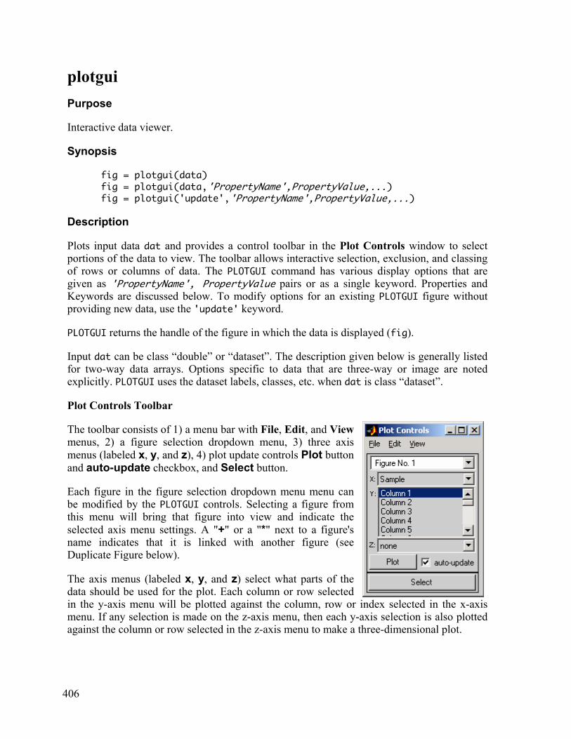
406

plotgui

Purpose

Interactive data viewer.

Synopsis fig = plotgui(data) fig = plotgui(data,'PropertyName',PropertyValue,...) fig = plotgui('update','PropertyName',PropertyValue,...)

Description

Plots input data dat and provides a control toolbar in the Plot Controls window to select portions of the data to view. The toolbar allows interactive selection, exclusion, and classing of rows or columns of data. The PLOTGUI command has various display options that are given as 'PropertyName', PropertyValue pairs or as a single keyword. Properties and Keywords are discussed below. To modify options for an existing PLOTGUI figure without providing new data, use the 'update' keyword.

PLOTGUI returns the handle of the figure in which the data is displayed (fig).

Input dat can be class “double” or “dataset”. The description given below is generally listed for two-way data arrays. Options specific to data that are three-way or image are noted explicitly. PLOTGUI uses the dataset labels, classes, etc. when dat is class “dataset”.

Plot Controls Toolbar

The toolbar consists of 1) a menu bar with File, Edit, and View menus, 2) a figure selection dropdown menu, 3) three axis menus (labeled x, y, and z), 4) plot update controls Plot button and auto-update checkbox, and Select button.

Each figure in the figure selection dropdown menu menu can be modified by the PLOTGUI controls. Selecting a figure from this menu will bring that figure into view and indicate the selected axis menu settings. A "+" or a "*" next to a figure's name indicates that it is linked with another figure (see Duplicate Figure below).

The axis menus (labeled x, y, and z) select what parts of the data should be used for the plot. Each column or row selected in the y-axis menu will be plotted against the column, row or index selected in the x-axis menu. If any selection is made on the z-axis menu, then each y-axis selection is also plotted against the column or row selected in the z-axis menu to make a three-dimensional plot.

407

If the input dat is three-way it is assumed to be a multivariate image, and the y-axis is slice or slab and the figure default is imagesc(dat(:,:,1)). This is also true if dat is class “dataset” with the type field set to 'image' or 'image'.

If the auto-update checkbox is selected, figures are updated automatically when new axis-menu selections are made. Otherwise, the Plot button must be pressed before any changes are reflected in the figure.

View Menu

Various options associated with the viewed data are contained in the View menu. The specific options depend on the data being plotted. The View menu options are listed below. Table: Opens a Plotted Data window that lists the numerical values of the

plotted data. Numbers: Displays the index number next to each plotted point. Labels: Displays available lables next to each plotted point. If no labels are

available this option is greyed out. Classes: Uses available class information to give each plotted point a different

symbol. If no class information is available this option is greyed out. Excluded Data: Shows any points which have been “excluded” from the data set. Axis Lines: Places lines through the origin. Auto Contrast: Contrast enhancement for a slice/slab for multivariate images (only

available when the data are 3-way). Interpolated Color: Interpolates colors for a slice/slab for multivariate images (only

available when the data are 3-way). Data Summary: Plots all the data, the mean, the standard deviation, or the mean ± the

standard deviation. For Variables (columns) or Samples (rows) depending on what is selected in the x-axis.

Rows: Plots the data across rows. Columns: Plots the data down the columns. Slabs: Uses IMAGESC to view a slice/slab of a 3-way array (only available when

the data are 3-way). Duplicate Figure: Creates a duplicate copy of the current figure that is linked to the current

figure i.e. if one figure is modified the other automatically changes to reflect the modification. The parent figure will have a "+" next to its name in the figure selection dropdown menu and the child figure will have a "*".

Spawn Figure: Creates a duplicate copy of the current figure that is not controled by the Plot Controls toolbar. This is a simple MATLAB figure.

Dock Controls: When checked, the Plot Controls toolbar are “docked” next to the controled figure.

Settings: Allows the user to modify other view settings.

408

Selection using the Select button

The Select button allows the user to select plotted points in the current figure. After clicking Select, the current figure will be brought to the front and points are selected using the current selection tool (see Edit menu below). To extend a selection (i.e. add new points to the already selected points), use the shift-key while pressing the mouse button. To remove points from the selection, use the control-key while pressing the mouse button. To keep from making any selection, press "Esc" or "Escape".

Edit Menu

The Edit menu contains various actions relating to selections. The specific actions available depends on the current selection and PLOTGUI mode. The Edit menu options are listed below. Select All: Selects all plotted points. Deselect All: Deselects all plotted points. Selection Mode: Menu used to choose selection mode from the following: Box: Click and drag a rubber band box around points, Polygon: Click to mark the corners of a polygon around points and

"Enter" to close the polygon, Paintbrush: Click and drag to "paint" a selection onto points, Single X: Click to select a single point on the x-axis, Single Y: Click to select a single point on the y-axis, X Range: Click and drag to select a range of points on the x-axis, Y Range: Click and drag to select a range of points on the y-axis, and Nearest: Click to select the nearest point. Exclude Selection: Excludes (soft deletes) the selected points from the data set. See

View/Excluded Data. Include Selection: Includes the selected points in the data set. See View/Excluded Data. Exclude Unselected: Exclude all unselected points from the data set i.e. keep only the

selected points. Info on Selection: Get information on selected point (only available when a single point is

selected). Set Class: Set the class of the selected points.

File Menu

The File menu contains various actions relating to files. The File menu options are listed below. Load Data: Creates an interface for the user to load data into PLOTGUI from the base

workspace or a file. Save Data: Creates an interface for the user to save data from PLOTGUI to the base

workspace or a file.

Properties and Keywords

409

The following is a list of available properties. Each should be included as a 'PropertyName', PropertyValue pair in an initial PLOTGUI call or a PLOTGUI 'update' call. Note that calls to PLOTGUI for 'PropertyName' and PropertyValue are case insensitive.

The current value of almost all properties can be retrieved using the getappdata function on the PLOTGUI figure and requesting the property of interest. Note that calls to GETAPPDATA are case sensitive and 'PropertyName' must be in all lower-case. The I/O format is:

currentvalue = getappdata(fig,'propertyname')

where fig is the handle of the PLOTGUI figure. If 'propertyname' is not included getappdata(fig) will list all the properties and their current values. Properties and their possible values follow: AxisMenuValues: {[x] [y] [z]}, Two or three element cell containing indices or

strings indicating which item, or items, to select in each of the three axis pull down menus. In [x] or [y] a value of 0 (zero) means to select index number. In [z] a value of 'none' means to not use the z-axis.

AxisMenuDefaults: Axis menu defaults are axis menu values used if the axis menu values can not be restored. The input format is the same as axismenuvalues.

Figure: [scalar integer], Figure on which data should be plotted {default is current figure}.

New: Key word – no associated PropertyValue. Creates a new figure for display of data. This is equivalent to an initial PLOTGUI call.

PlotBy: [scalar integer], Dimension (mode) for the axis menu selections: 0 = data summary, 1 = rows, 2 = columns, etc. (see View menu). The default is 2 or the number of modes in the data if larger than 2-way.

VSIndex: [ 1 1] {default}, Two element vector indicating if "Index" should be offered on x and y axis menus. A 1 indicates that it should be offered as a selection and a 0 indicates that it should not e.g. [1 1] indicates that it should be offered for both the x-axis and y-axis.

The following are image specific properties: Image: Key word – no associated PropertyValue. Unfolds a 2 or 3-way

array and displays it as and image, allowing selection, classing, and exclusion of individual pixels.

Unfold: Key word – no associated PropertyValue. Pseudonym for “image”. AsImage: Key word – no associated PropertyValue. Display 3-way data that

have already been unfolded as an image allowing selection, classing, and exclusion of individual pixels.

The following are view properties: ViewClasses: [1] {default}, Turns on View/Classes menu. A 0 (zero) turns it off.

410

ViewExcludedData: [1] {default}, Turns on View/Excluded Data menu. A 0 (zero) turns it off.

ViewLabels: [1] {default}, Turns on View/Labels menu. A 0 (zero) turns it off. ViewNumbers: [1] {default}, Turns on View/Numbers menu. A 0 (zero) turns it off. The following are plot properties: LineStyle: <string>, Defines line style (see PLOT). PlotType: <string>, String used to select plot type {default [ ] is atuomatic

selection}. Other values are 'scatter', 'bar', 'none' ('none' = do no plotting).

SelectionMarker: <string>, Defines marker style for selected points (see PLOT). The following are selection properties: SelectionMode: <string>, Defines the selection mode. This can be any string listed

under View/Selection Mode above. Also see GSELECT. BrushWidth: [scalar integer number of pixels], This defines the brush width

for use when selectionmode = 'paintbrush'. See View/Selection Mode/Paintbrush.

NoSelect: [0] {default}, When set to 0 this allows selections. When set to 1 no selection is allowed.

NoInclud: [0] {default}, When set to 0 this allows changes to the inlclud field (i.e. it allows data to be excluded). When set to 1 no changes to the inlclud field are allowed (i.e. data can not be excluded).

The following are on-event properties: CloseGUICallback: Command(s) to execute when the figure is closed. IncludChangeCallback: Command executed when includ field of the dataset is

modified. InfoReqCallback: Command executed when information on a selected point is

requested. PlotCommand: Command executed after plotting (e.g. draw limits, assign

ButtonDownFcns, modifiy axes, …). SelectionChangeCallback: Command executed when a selction is made. SetClassCallback: Command executed when the class field of the dataset is changed. The following are confidence limit properties: ConfLimits: Boolean flag to make "Conf. Limits" controls visible. 1 = show controls

(PLOTGUI does nothing with these controls, thus the routine specified in 'plotcommand' must be set to use values).

LimitsValue: Value for Conf. Limits editbox. ShowLimits: Value for "Conf. Limits" checkbox (1 = checked). The following are figure linking properties (WARNING! Modifying these settings can lead to unexpected results!): Children: Add new child of the current PLOTGUI figure (all child figures are

updated when their parent is updated and closed when their parent is

411

closed). Note: this property will only allow adding of additional children. Other modifications must be made using setappdata.

ControlBy: Reassign control for PLOTGUI figure. Parent: Assign a parental link (Forces the parent figure to update if this figure is

updated, also see 'Children'). TimeStamp: Time-stamp of last time this figure was updated (can be set to any string

to isolate figure from updating by parents). The following are other miscellaneous properties: UIControl: Add extra uicontrol(s) to PLOTGUI control toolbar for use with current

figure (buttons, sliders, etc.). The value passed to UIControl should be a cell in which each entry is the tag of a new object to create and the value of that field should contain a cell of uicontrol property / value pairs to set for that object. For example:

myobj.mybtn = {'style', 'pushbutton', 'string', 'new fig', 'callback', 'figure'};

plotgui('update','uicontrol',myobj) creates a button with the tag 'mybtn' on the controls for the current

figure. If the cell for any object does not contain a 'position' property for the

object, PLOTGUI will manage the object's position. The following are read-only properties. These properties can only be viewed and are only accessible through the MATLAB getappdata command. Selection: Cell array of currently selected values. Usually the same format as

"includ" field of DataSet object where each cell represents the index of selected items in each dimension {rows, columns, slabs, ...}.

When selecting elements in greater than 2-dimensional data (and without the use of the 'image' keyword), two cells of this field will be pairs of selected indices: {x,y,[]} or {[],y,z}.

FigureType: 'PlotGUI' DataSet: DataSet used in figure (or pointer to figure with actual dataset) Note: This is set by calling PLOTGUI with a new dataset as an input. The

actual DataSet can be retrieved using the getdataset command (see below).

The following are other valid figure properties. See the MATLAB doc umentation on FIGURE properties for additional information. HandleVisibility, MenuBar, Name, NumberTitle, Position, Resize, Tag, ToolBar, Units, UserData, Visible, WindowStyle

Examples

fig = plotgui(mydata) plots mydata allowing user to select which column(s) of mydata to plot using pull-down menus. Figure number of plot is returned.

412

plotgui(mydata,'plotby',1) or plotgui(mydata,'plotby','rows') plots mydata as in first example except that rows of mydata (dimension 1) are used for pull-down menus instead of columns. Note: When a PLOTGUI property is set for a given figure, the new value will be retained until a new value for that property is provided, even if new data is plotted on the same PLOTGUI figure.

fig = plotgui(mydata,'plotby',1,'axismenuvalues',{[1] [2 3]}) plots rows of mydata; sets controls with row 1 selected for the x-axis and rows 2 and 3 selected for the y-axis. Use:

getappdata(fig,'axismenuvalues') to retrieve current axis menu settings. axispulldown

plotgui(mydata,'viewclasses',1) plots mydata using symbols to identify the classes stored in dataset mydata. Use a value of 0 (zero) to turn off viewclasses.

plotgui('update','viewclasses',1) Turns on viewclasses property for current figure without having to pass data to plot (substitute string 'update' for data)

mydata = plotgui('getdataset',fig) Retrieves mydata from figure fig.

plotgui(myimage,'image') plots 3-way image myimage selecting slabs of the image for display. The keyword 'image' allows selection, classing and exclusion of pixels in the image.

See Also

dataset, analysis, plotloads, plotscores

413

plotloads Purpose

Extract and display loadings information from model.

Synopsis a = plotloads(modl,options) a = plotloads(loads,labels,classes) options = plotloads('options')

Description

Given a standard model structure, relevant loading information (e.g. labels) is collected and passed to PLOTGUI for plotting. The input is the model containing loadings to plot modl. (e.g. see MODELSTRUCT). Optional input options is discussed below.

Input loads is a N by K loadings matrix (class “double”). Optional input labels is a character or cell array with N rows containing sample labels, and optional input classes is a vector with N integer elements of class identifiers.

If no output is requested then PLOTLOADS initiates an interactive plotting utility to make loadings plots. If an output is requested, no plots are made, and the output a is a dataset object containing the loadings and labels, etc.

Options options = a structure array with the following fields: name: 'options', name indicating that this is an options structure, display: [ {'on'} | 'off' ], governs level of display, plots: ['none' | 'final' | {'auto'} |], governs plotting behavior,

'auto' makes plots if no output is requested {default}, and figure: [],governs where plots are made, when figure = [] plots are made in

a new figure window {default}, this can also be a valid figure number (i.e. figure handle).

The default options can be retreived using: options = plotloads('options');.

See Also

analysis, modelstruct, pca, pcr, plotgui, plotscores, pls

414

plotscores Purpose

Extract and display scores information from model.

Synopsis a = scoresplot(modl,options) a = scoresplot(modl,pred,options) a = plotscores(scores,labels,classes) options = plotscores('options')

Description

Given a standard model structure, relevant scores information (e.g. labels) is collected and passed to PLOTGUI for plotting. The input is the model containing scores to plot modl. (e.g. see MODELSTRUCT). A second input pred contains a test or validation structrure (see PCA) that can be plotted with scores in modl. Optional input options is discussed below.

Input scores is a M by K scores matrix (class “double”). Optional input labels is a character or cell array with M rows containing sample labels, and optional input classes is a vector with M integer elements of class identifiers.

If no output is requested then PLOTSCORES initiates an interactive plotting utility to make scores plots. If an output is requested, no plots are made, and the output a is a dataset object containing the scores and labels, etc.

Options options = a structure array with the following fields: name: 'options', name indicating that this is an options structure, display: [ {'on'} | 'off' ], governs level of display, plots: ['none' | 'final' | {'auto'} |], governs plotting behavior,

'auto' makes plots if no output is requested {default}, figure: [],governs where plots are made, when figure = [] plots are made in

a new figure window {default}, this can also be a valid figure number (i.e. figure handle), and

sct: [ 0 | {1} ], tells whether to plot cal (modl scores) with test (pred scores), sct = 1 plots original calibration data with prediction set {default}.

The default options can be retreived using: options = plotscores('options');.

See Also

analysis, modelstruct, pca, pcr, plotgui, plotloads, pls

415

pls Purpose

Partial least squares regression for univariate or multivariate y-block.

Synopsis model = pls(x,y,ncomp,options) %calibration pred = pls(x,model,options) %prediction valid = pls(x,y,model,options) %validation options = pls('options')

Description

PLS calculates a single partial least squares regression model using the given number of components ncomp to predict y from measurements x.

To construct a PLS model, the inputs are x the predictor block (2-way array class “double” or class “datadet”), y the predicted block (2-way array class “double” or class “datadet”), ncomp the number of components to to be calculated (positive integer scalar), and the optional structure, options. The output is a standard model structure model with the following fields (see MODELSTRUCT): modeltype: 'PLS', datasource: structure array with information about input data, date: date of creation, time: time of creation, info: additional model information, reg: regression vector, loads: cell array with model loadings for each mode/dimension, pred: 2 element cell array with model predictions for each input block (when

options.blockdetail='normal' x-block predictions are not saved and this will be an empty array) and the y-block predictions.

wts: double array with X-block weights, tsqs: cell array with T2 values for each mode, ssqresiduals: cell array with sum of squares residuals for each mode, description: cell array with text description of model, and detail: sub-structure with additional model details and results.

To make predictions the inputs are x the new predictor x-block (2-way array class “double” or “dataset”), and model the PLS model. The output pred is a structure, similar to model, that contains scores, predictions, etc. for the new data.

416

If new y-block measurements are also available then the inputs are x the new predictor x-block (2-way array class “double” or “dataset”), y the new predicted block (2-way array class “double” or “dataset”), and model the PLS model. The output valid is a structure, similar to model, that contains scores, predictions, and additional y-block statistics etc. for the new data.

Note: Calling pls with no inputs starts the graphical user interface (GUI) for this analysis method.

Options options = a structure array with the following fields: name: 'options', name indicating that this is an options structure, display: [ 'off' | {'on'} ], governs level of display to command window, plots [ 'none' | {'final'} ], governs level of plotting, outputversion: [ 2 | {3} ], governs output format (see below), preprocessing: {[] []}, two element cell array containing preprocessing structures (see

PREPROCESS) defining preprocessing to use on the x- and y-blocks (first and second elements respectively)

algorithm: [ 'nip' | {'sim'} ], PLS algorithm to use: NIPALS or SIMPLS {default}, and

blockdetails: [ {'standard'} | 'all' ], extent of predictions and residuals included in model, 'standard' = only y-block, 'all' x- and y-blocks.

The default options can be retreived using: options = pls('options');.

OUTPUTVERSION

By default (options.outputversion = 3) the output of the function is a standard model structure model. If options.outputversion = 2, the output format is:

[b,ssq,p,q,w,t,u,bin] = pls(x,y,ncomp,options)

where the outputs are b = matrix of regression vectors or matrices for each number of principal

components up to ncomp, ssq = the sum of squares information, p = x-block loadings, q = y-block loadings, w = x-block weights, t = x-block scores u = y-block scores, and bin = inner relation coefficients.

417

Note: The regression matrices are ordered in b such that each Ny (number of y-block variables) rows correspond to the regression matrix for that particular number of principal components.

Algorithm

Note that unlike previous versions of the PLS function, the default algorithm (see Options, above) is the faster SIMPLS algorithm. If the alternate NIPALS algorithm is to be used, the options.algorithm field should be set to 'nip'.

See Also

crossval, modelstruct, pcr, plsnipal, preprocess, analysis, ridge

418

plsda Purpose

Partial least squares discriminate analysis.

Synopsis model = plsda(x,y,ncomp,options) model = plsda(x,ncomp,options) pred = plsda(x,model,options) valid = plsda(x,y,model,options) options = plsda('options')

Description

PLSDA is a multivariate inverse least squares discrimination method used to classify samples. The y-block in a PLSDA model indicates which samples are in the class(es) of interest through either:

(A) a column vector of class numbers indicating class asignments:

y = [1 1 3 2]';

(B) a matrix of one or more columns containing a logical zero (= not in class) or one (= in class) for each sample (row): y = [1 0 0; 1 0 0; 0 0 1; 0 1 0]

NOTE: When a vector of class numbers is used (case A, above), class zero (0) is reserved for "unknown" samples and, thus, samples of class zero are never used when calibrating a PLSDA model. The model will include predictions for these samples.

The prediction from a PLSDA model is a value of nominally zero or one. A value closer to zero indicates the new sample is NOT in the modeled class; a value of one indicates a sample is in the modeled class. In practice a threshold between zero and one is determined above which a sample is in the class and below which a sample is not in the class (See, for example, PLSDTHRES). Similarly, a probability of a sample being inside or outside the class can be calculated using DISCRIMPROB. The predicted probability of each class is included in the output model structure in the field:

model.details.predprobability

INPUTS x = X-block (predictor block) class "double" or "dataset",

419

y = Y-block - OPTIONAL if x is a dataset containing classes for sample mode (mode 1) otherwise, y is one of: (A) column vector of sample classes for each sample in x -OPTIONAL

if x is a dataset containing classes for sample mode (mode 1) or (B) a logical array with 1 indicating class membership for each sample

(rows) in one or more classes (columns) ncomp = the number of latent variables to be calculated (positive integer scalar). OUTPUT model = standard model structure containing the PLSDA model (See

MODELSTRUCT). pred = structure array with predictions valid = structure array with predictionsz

Note: Calling plsda with no inputs starts the graphical user interface (GUI) for this analysis method.

Options

display: [ 'off' | {'on'} ] governs level of display to command window.

plots: [ 'none' | {'final'} ] governs level of plotting.

preprocessing: {[] []} preprocessing structures for x and y blocks (see PREPROCESS).

algorithm: [ 'nip' | {'sim'} ] PLS algorithm to use: NIPALS or SIMPLS

blockdetails: [ 'compact' | {'standard'} | 'all' ] Extent of detail included in model.

'standard' keeps only y-block, 'all' keeps both x- and y- blocks

See Also

class2logical, crossval, pls, plsdthres, simca

420

plsdaroc Purpose

Calculate and display ROC curves for PLSDA model.

Synopsis roc = plsdaroc(model,ycol,options)

Description

ROC curves can be used to assess the specificity and sensitivity possible with different predicted y-value thresholds for a PLSDA model. Inputs are a PLSDA model model, an optional index into the y-columns used in the model ycol [default = all columns], and an options structure. Output is a dataset with the sensitivity/specificity data roc.

Options plots : [ 'none' | {'final'}] governs plotting on/off

See Also

discrimprob, plsda, plsdthres, simca

421

plsdthres Purpose

Bayesian threshold determination for PLS Discriminate Analysis.

Synopsis [threshold,misclassed,prob] = plsdthres(model,options) [threshold,misclassed,prob] = plsdthres(y,ypred,cost,prior,out)

Description

PLSDTHRES uses the distribution of calibration-sample predictions obtained from a PLS model built for two or more logical classes to automatically determine a threshold value which will best split those classes with the least probability of false classifications for future predictions. It is assumed that the predicted values for each class are approximately normally distributed. The calibration can contain more than 2 classes, in which case thresholds to distinguish all classes will be determined. It is assumed that with more than 2 classes the primary misclassification threat is from the adjacent class(es).

INPUTS y = measured Y-block values used in PLS, and ypred = PLS predicted Y values for calibration samples.

OPTIONAL INPUTS cost = [], vector of logarithmic cost biases for each class in y, cost is used to

bias against misclassification of a particular class or classes {default = [] uses all zeros i.e. equal cost}.

prior = [], vector of prior probabilities of observing each class. If any class prior is Inf, the frequency of observation of that class in the calibration is used as its prior probability. If all priors are Inf, this has the effect of providing the fewest incorrect predictions assuming that the probability of observing a given class in future samples is similar to the frequency that class in the calibration set. {default = [] uses all ones i.e. equal priors.}

out = [ {0} | 1], governs plotting, out=1 provide plots of thresholding, out=0 makes no plots.

OUTPUTS threshold = [], vector of thresholds. If y consists of more than two classes, threshold

will be a vector giving the upper bound y-value for each class. misclassed = [], array containing the fraction of misclassifications for each class

(rows): Column 1 = false negatives and Column 2 = false positives.

422

prob = lookup matrix of predicted y (column 1) vs. probability of each class (columns 2 to end).

See Also

crossval, discrimprob, pls, simca

423

plsnipal Purpose

Calculate single latent variables for partial least squares regression.

Synopsis [p,q,w,t,u] = plsnipal(x,y)

Description

PLSNIPAL is called by the routine pls to calculate each latent variable in a partial least squares regression.

Inputs x and y are either the x-block and y-block for calculation of the first latent variable, or the x-block and y-block residuals for calculation of subsequent latent variables.

The outputs are p the x-block latent variable loadings, q the y-block variable loadings, w the x-block latent variable weights, t the x-block latent variable scores, and u the y-block latent variable scores.

See Also

nippls, pls, analysis, simpls

424

plspulsm Purpose

Builds finite impulse response (FIR) models for multi-input single (MISO) output systems using partial least squares regression.

Synopsis b = plspulsm(u,y,n,maxlv,split,delay)

Description

plspulsm calculates a vector of FIR coefficients b using PLS regression. Inputs are a matrix of process input vectors u, and a process output vector y. n is a row vector with the number of FIR coefficents to use for each input, maxlv is the maximum number of latent variables to consider, split is the number of times the model is rebuilt and tested during cross-validation, and delay is a row vector containing the number of time units of delay for each input.

Note: plspulsm uses contiguous blocks of data for cross-validation.

Examples

b = plspulsm([u1 u2],y,[25 15],5,10,[0 3])

This system has 2 inputs as column vectors u1 and u2 and a single output vector y. The FIR model will use 25 coefficients for input variable u1 and 15 coefficients for input variable u2. For this model a maximum of 5 latent variables will be considered. The cross validation split the data into 10 subsets. The number of time units of delay for the first input variable u1 is 0 and for the second input variable u2 it is 3.

See Also

autocor, crosscor, fir2ss, wrtpulse

425

plsrsgcv Purpose

Generates a matrix used to calculate residuals from a single data block using partial least squares regression models with cross vaildation.

Synopsis coeff = plsrsgcv(data,lv,cvit,cvnum,out)

Description

coeff = plsrsgncv(data,lv,cvit,cvnum) calculates a matrix coeff from a single data block data. plsrsgncv calculates partial least squares regression models of each variable in the matrix data using the remaining variables and cross-validation with random test data blocks. The maximum number of latent variables to consider is lv, the number of test sets is cvit, and the number of samples in each test set is cvnum. Multiplying a new data matrix by the matrix coeff yields a matrix whose values are the difference between the new data and it's prediction based on the PLS regressions created by plsrsgncv.

See Also

plsrsgn, replace

426

plsrsgn Purpose

Generates a matrix used to calculate residuals from a single data block using partial least squares regression models.

Synopsis coeff = plsrsgn(data,lv,out)

Description

coeff = plsrsgn(data,lv) calculates a matrix coeff from a single data block data. plsrsgn calculates partial least squares regression models of each variable in the matrix data using the remaining variables and the number of latent variables lv. Multiplying a new data matrix by the matrix coeff yields a matrix whose values are the difference between the new data and it's prediction based on the PLS regressions created by plsrsgn.

See Also

plsrsgcv, replace

427

plttern Purpose

Plots a 2D ternary diagram.

Synopsis [tdata,h] = plttern(data,linestyle,x1lab,x2lab,x3lab)

Description

PLTTERN makes 2-D ternary plots of the data contained in the three column input matrix data. The columns of data correspond to concentrations ( ≥ 0 and real) and are normalized to fit in the range 0 to 100. Optional inputs x1lab, x2lab, x3lab are row vectors of text containing labels for the axes. The output tdata is the normalized concentration data.

See Also

dp, ellps, hline, pan, pltternf, vline, zline

428

pltternf Purpose

Plots a 3D ternary diagram with frequency of occurrence.

Synopsis tdata = plttern(data,x1lab,x2lab,x3lab);

Description

PLTTERN makes 3-D ternary plots of the data contained in the four column input matrix data. The first three columns of data correspond to concentrations ( ≥ 0 and real) and are normalized to fit in the range 0 to 100. The fourth column of data corresponds to the frequency of occurrence ( ≥ 0 and real). Optional inputs x1lab, x2lab, x3lab are row vectors of text containing labels for the axes. The output tdata is the normalized concentration data.

See Also

dp, ellps, hline, pan, plttern, vline, zline

429

polyinterp Purpose

Polynomial interpolation, smoothing, and differentiation.

Synopsis yi = polyinterp(x,y,xi,width,order,deriv);

Description

For a M by N input matrix y with corresponding 1 by N axis vector x (the points at which the y are given) POLYINTERP estimates the M by N matrix yi which has the smoothed values of y. If the points are evenly spaced use the SAVGOL function instead. Note that y is a matrix of ROW vectors to be smoothed.

Optional inputs are xi a vector of points to interpolate to, width specifies the number of points in the filter {default = 15}, the order of the polynomial order {default = 2}, and the derivative deriv {default = 0}.

Examples

If y is a 5 by 100 matrix, x is a 1 by 100 vector, and xi is a 1 by 91 vector then polyinterp(x,y,xi,11,3,1) gives the 5 by 91 matrix of first-derivative row vectors resulting from an 11-point cubic interpolation to the 91 points in xi.

See Also

baseline, lamsel, mscorr, savgol, stdfir

430

polypls Purpose

Calculate partial least squares regression models with polynomial inner relations.

Synopsis [p,q,w,t,u,b,ssqdif] = polypls(x,y,lv,n)

Description

POLYPLS creates a partial least squares regression model with polynomial fit for the inner relation. Inputs are a matrix of predictor variables (x-block) x, a matrix of predicted variables (y-block) y, the number of latent variables lv, and the order of the polynomial n.

Outputs are p the x-block latent variable loadings, q the y-block variable loadings, w the x-block latent variable weights, t the x-block latent variable scores, u the y-block latent variable scores, b a matrix of polynomial coefficients for the inner relationship, and ssqdif a table of x- and y-block variance captured by the PLS model.

Use POLYPRED to make predictions with new data.

See Also

lwrxy, pls, polypred

431

polypred Purpose

Make predictions for partial least squares regression models with polynomial inner relations.

Synopsis ypred = polypred(x,b,p,q,w,lv)

Description

POLYPRED uses parameters created by the routine POLYPLS to make predictions from a new x-block matrix of predictor variables x. Inputs are b a matrix of polynomial coefficients for the inner relationship, p the x-block latent variable loadings, q the y-block variable loadings, w the x-block latent variable weights, and the number of latent variables lv.

Note: It is important that the scaling of the new data x is the same as that used to create the model parameters in POLYPLS.

See Also

lwrxy, polypls, pls

432

preprocess Purpose

Selection and application of preprocessing methods.

Synopsis s = preprocess(s) %GUI preprocessing selection s = preprocess('default','methodname') %Non-GUI selection [datap,sp] = preprocess('calibrate',s,data) %single block calibrate [datap,sp] = preprocess('calibrate',s,xblock,yblock) %multi-block datap = preprocess('apply',sp,data) %apply to new data data = preprocess('undo',sp,datap) %undo preprocessing

Description

PREPROCESS is a general tool to choose preprocessing steps and to perform these steps on data. See PREPROUSER for a description on how custom preprpocessing can be added to the standard proprocessings listed below. PREPROCESS has four basic command-line forms which include:

1) SELECTION OF PREPROCESSING.

The purpose of the following calls to PREPROCESS is to generate standard structure arrays that contain the desired preprocessing steps.

s = preprocess;

generates a GUI and allows the user to select preprocessing steps interactively. The output s is a standard preprocessing structure.

s = preprocess(s);

allows the user to interactively edit a previously identified preprocessing structure s. The output s is the edited preprocessing structure.

s = preprocess('default','methodname');

returns the default structure for method 'methodname'. A list of strings that can be used for 'methodname' can be viewed using the command:

preprocess('keywords')

A list of standard methods 'methodname' follow: 'abs': takes the absolute value of the data (see ABS), 'autoscale': centers columns to zero mean and scales to unit variance (see AUTO), 'detrend': remove a linear trend (see BASELINE),

433

'gls weighting': generalized least squares weighting (see GLSW), 'groupscale': group/block scaling (see GSCALE), 'mean center': center columns to have zero mean (see MNCN), 'msc (mean)': multiplicative scatter correction with offset, the mean is the reference

spectrum (see MSCORR), 'median center': center columns to have zero median (see MEDIAN), 'normalize': normalization of the rows (see NORMALIZ), 'osc': orthogonal signal correction (see OSCCALC and OSCAPP), 'sg': Savitsky-Golay smoothing and deriviatives (see SAVGOL), and 'snv': standard normal deviate (autoscale the rows, see SNV).

The output is a standard preprocessing structure array s where each method to apply is a separate record.

2) CALIBRATE.

The objective of the following calls to PREPROCESS is to estimate preprocessing parameters, if any, from a calibration data set and perform preprocessing on the calibration data set. The I/O format is:

[datap,sp] = preprocess('calibrate',s,data);

The inputs are s a standard preprocessing structure and data the calibration data. The preprocessed data is returned in datap, and preprocessing parameters are returned in a modified preprocessing structure sp. Note that sp is used as an input with the 'apply' and 'undo' commands described below.

Short cuts for each method can also be used. Examples for 'mean center' and 'autoscale' are

[datap,sp] = preprocess('calibrate','mean center',data); [datap,sp] = preprocess('calibrate','autoscale',data);

Preprocessing for some multi-block methods require that the y-block be passed also. The I/O format in these cases is:

[datap,sp] = preprocess('calibrate',s,xblock,yblock);

Preprocessing 'methodname' that require a y-block are: 'osc' 'gls weighting'

3) APPLY.

The objective of the following call to PREPROCESS datap = preprocess('apply',sp,data)

434

is to apply the calibrated preprocessing in sp to new data. Inputs are sp the modified preprocessing structure (See 2 above) and the data, data, to apply the preprocessing to. The output is preprocessed data datap that is class “dataset”.

4) UNDO.

The inverse of applying preprocessing is perfromed in the following call to PREPROCESS data = preprocess('undo',sp,datap);

Inputs are sp the modified preprocessing structure (See 2 above) and the data, datap, (class “double” or “dataset”) from which the preprocessing is removed. Note that for some preprocessing methods an inverse does not exist or has not been defined and an 'undo' call will cause an error to occur. For example, 'osc' and 'sg'. One reason for not defining an inverse, or undo, is because it would require a significant amount of memory storage when data sets get large.

See Also

crossval, pca, pcr, pls, preprouser

435

preprouser Purpose

User defined items for preprocess catalog.

Synopsis preprouser(fig)

Description

Each method available in the preprocess function has an associated 'methodname' such as those listed in the help for preprocess. Each method is defined using a preprocessing structure that contains all the necessary information to perform calculations for that method. The standard methods are defined in the preprocatalog file, which should not be edited by the user. Additional user-defined methods can be defined in the preprouser file and the following text describes how the user to add custom preprocessing methods. A few example methods already exist in the preprouser file to guide the user.

To add a custom user-defined preprocessing method, the user must 1) open the PREPROUSER.M file, 2) edit the file to create a structure with the fields described below, 3) after defining the structure add the line preprocess('addtocatalog',fig,usermethod), and 4) save and close the PREPROUSER.M file.

The line added in Step 3 preprocess('addtocatalog',fig,usermethod)

makes the new custom method available to PREPROCESS. The input usermethod is the preprocessing structure containing the user-defined method, and fig is a figure handle passed to preprouser by preprocess.

The methods defined in the preprocatalog and preprouser files are available to all functions making use of the preprocess function.

The fields in a preprocessing structure are listed here. Detailed descriptions and examples follow this list. description: text string containing a description for the method, calibrate: cell containing the line(s) of code to execute during a calibration

operation (see command-line form 2 of PREPROCESS), apply: cell containing the line(s) of code to execute during an apply operation

(see command-line form 3 of PREPROCESS), undo: cell containing the line(s) of code to execute during an undo operation

(see command-line form 4 of PREPROCESS),

436

out: cell used to hold calibration-phase results for use in apply or undo (these are the parameters estimated from the calibration data and used to preprocess new data),

settingsgui: text string containing the function name of a method-specific GUI to invoke when the Settings button is pressed in the preprocessing GUI,

settingsonadd: [ 0 | {1} ], boolean: 1 = indicates that the settings GUI should be automatically brought up when method is "added" in the preprocessing GUI,

usesdataset: [ {0} | 1 ], boolean: indicates if this method should be passed a dataset object (1) or a an array (0) (e.g. class “double” or “uint8”),

caloutputs: integer: number of expected items in field out after calibration has been performed. This field is set by the user to tell PREPROCESS what the length of the cell in field out will be after calibration,

keyword: text string containing the 'methodname', this string is used in the call to PREPROCESS so that it will return the custom preprocessing structure (see command-line form 1 of PREPROCESS), and

userdata: user-defined variable often used to store method options.

Detailed descriptions and examples for each field follow:

DESCRIPTION:

The description is a short (1-2 word) text string containing a description for the preprocessing method. The string will be displayed in the GUI and can also be used as a string keyword (see also keyword) to refer to this method.

example: pp.description = 'Mean Center';

CALIBRATE, APPLY, UNDO:

Each of these “command” fields contains a single cell consisting of a command string to be executed by PREPROCESS when performing calibration, apply, or undo operations (see command-line forms 2, 3, and 4 of PREPROCESS). Calibrate actions operate on original calibration data with the output parameters stored in the out field, whereas apply actions operate on new data using parameters stored in the out field as input(s). For methods which act on a single sample at a time, the calibrate and apply operations are often identical (for example, see the normalize example below). The undo action uses parameters stored in the out field as input(s) to remove preprocessing from previously preprocessed data. However, the undo action may be undefined for certain methods. If this is the case, the undo field should be an empty cell.

To assure that all samples (rows) in the data have been appropriately preprocessed, an apply command is automatically performed following a calibrate call. Note that excluded variables are replaced with NaN.

437

The command strings should be one or more valid MATLAB commands, each separated by a semicolon ';' (e.g. see EVAL). Each command will be executed inside the PREPROCESS environment in which the following variables are available: data: The data field contains the data on which to operate and in which to

return modified results. If the field usesdataset is 1 (one) then data will be a DataSet object.

In this case, it is expected that the function will calibrate using only included rows but apply and undo the preprocessing to all rows.

If the field usesdataset is 0 (zero) then data will be an array (e.g. class “double”). In this case, the function will calibrate using all rows and columns and will apply and undo the preprocessing to all rows and columns.

out: Contents of the preprocessing structure field out (described below). Any changes will be stored in the preprocessing structure for use in subsequent apply and undo commands.

userdata: Contents of the preprocessing structure field userdata (described below). Any changes will be stored in the preprocessing structure for later retrieval.

Several variables are available for use during command operations (calibarate, apply, and undo). However, these variables should not be changed by the commands and are considered “read-only”. include: When the field usesdataset = 1, the data is passed as a dataset object.

In this case, include contains the contents of the original dataset object’s includ field.

otherdata: Cell array of any inputs to PREPROCESS which followed the data in the input list. For example, it is used by PLS_Toolbox regression functions to pass the y-block for use in methods which require that information.

originaldata: A dataset object which contains the original data unmodified by any preprocessing steps. For example, originaldata can be used to retrieve axis scale or class information even when usesdataset is 0 (zero).

Examples:

The following calibrate field performs mean-centering on data, returning both the mean-centered data as well as the mean values which are stored in out{1}:

pp.calibrate = { '[data,out{1}] = mncn(data);' };

The following apply and undo fields use the scale and rescale functions to apply and undo the previously determined mean values (stored by the calibrate operation in out{1}) with new data:

pp.apply = { 'data = scale(data,out{1});' }; pp.undo = { 'data = rescale(data,out{1});' };

OUT:

438

The out field is a cell array that contains the output parameters returned during the calibration operation. For example, if the following commands are run

load wine s = preprocess('default','autoscale'); [dp,sp] = preprocess('calibrate',s,wine);

then the out field of sp is a 1 by 2 cell array with the first cell, out{1}, containing the means of the variables in the dataset wine, and the second cell, out{2}, contains the standard deviations. These parameters are used in subsequent apply and undo commands. See the related field caloutputs. Prior to the calibration operation both the out and caloutputs fields are empty.

SETTINGSGUI:

The name of a graphical user interface (GUI) function that allows the user to set options for this method. The function is expected to take as its only input a standard preprocessing structure from which it should take the current settings. The function should output the same preprocessing structure modified to meet the user's specification. Typically, these changes are made to the userdata field and the commands in the calibrate, apply and undo fields use that field’s contents as input options.

The design of GUIs for selection of options is beyond the scope of this document and the user is directed to the following example files, both of which use GUIs to modify the userdata field of a preprocessing structure: autoset.m savgolset.m .

Example: pp.settingsgui = 'autoset';

SETTINGSONADD:

The settingsonadd field contains a boolean (1=true, 0=false) value. If it is 1=true, then when the user adds the method in the PREPROCESS GUI, the method's settingsgui will be automatically invoked. If a method requires the user to make a selection of options, settingsonadd=1 will guarantee that the user has an opportunity to modify the options or at least choose the default settings.

Example: pp.settingsonadd = 1;

USESDATASET:

The usesdataset field contains a boolean (1=true, 0=false) value.

If it is 1=true, the preprocessing method is capable of handling dataset objects and PREPROCESS will pass the data as a dataset. It is the responsibility of the function(s) called by the method to appropriately handle the dataset’s includ field.

439

If it is 0=false, the preprocssing method expects standard MATLAB classes (double, uint8, etc). PREPROCESS, which uses a dataset object internally to hold the data, will extract data from the dataset ojbect prior to calling this method. It will then reinsert the preprocessed data back into the dataset object after the method has been invoked.

Although excluded columns are never extracted and excluded rows are not extracted when performing calibration operations, excluded rows are passed when performing apply and undo operations.

Example: pp.usesdataset = 0;

CALOUTPUTS:

For functions which require a calibrate operation prior to an apply or undo (see the fields: calibrate and out), this field indicates how many values are expected in the out field. For example, in the case of mean centering the mean values stored in the field out are required to apply or undo the operation. Initially, out is an empty cell ({}). Following the calibration operation for mean centering, it becomes a single-item cell (length of one). For other calibration operations out may be a cell of length greater than one.

By examining this cell’s length, PREPROCESS can determine if a preprocessing structure has already been calibrated and contains the necessary information. The caloutputs field, when greater than zero, indicates to PREPROCESS that it should test the out field prior to attempting an apply or undo.

Example: in the case of mean-centering, the length of out should be 1 (one) after calibration. pp.caloutputs = 1;

KEYWORD:

The field keyword is a string that can be used to retrieve the default preprocessing structure for this method. When retrieving a structure by keyword, PREPROCESS ignores any spaces and is case-insensitive. The keyword field (or the description string, discussed above) can be used in place of any preprocessing structure in calibrate and default calls to preprocess:

pp = preprocess('default','meancenter');

Example: pp.keyword = 'mncn';

USERDATA:

The field userdata contains additional user-defined data that can be changed during a calibration operation and retrieved for use in apply and undo operations. This field is often

440

used to hold options for the preprocessing method which are then used by the commands in the calibrate, apply, and undo fields.

Example: in SAVGOL several input variables are defined with various method options, then they are assembled into a vector in userdata:

pp.userdata = [windowsize order derivative];

Examples

The following is the preprocessing structure used for sample normalization (see NORMALIZ). The calibrate and apply commands are identical and there is no information that is stored during the calibration phase, thus caloutputs is zero. There is no undo defined for this operation (this is because the normalization information required to undo the action is not being stored anywhere). The norm type (e.g. a 2-norm) of the normalization is set in userdata and is used in both calibrate and apply steps.

pp.description = 'Normalize'; pp.calibrate = {'data = normaliz(data,0,userdata(1));'}; pp.apply = {'data = normaliz(data,0,userdata(1));'}; pp.undo = {}; pp.out = {}; pp.settingsgui = 'normset'; pp.settingsonadd = 0; pp.usesdataset = 0; pp.caloutputs = 0; pp.keyword = 'Normalize'; pp.userdata = 2;

The following is the preprocessing structure used for Savitsky-Golay smoothing and derivatives (see SAVGOL). In many ways this structure is similar to the normalize structure except that SAVGOL takes a dataset object as input and, thus, usesdataset is set to 1. Also note that because of the various settings required by savgol, this method uses of the settingsonadd feature to bring up the settings GUI as soon as the method is added.

pp.description = 'SG Smooth/Derivative'; pp.calibrate =

{'data=savgol(data,userdata(1),userdata(2),userdata(3));'}; pp.apply =

{'data=savgol(data,userdata(1),userdata(2),userdata(3));'}; pp.undo = {}; pp.out = {}; pp.settingsgui = 'savgolset'; pp.settingsonadd = 1; pp.usesdataset = 1; pp.caloutputs = 0; pp.keyword = 'sg'; pp.userdata = [ 15 2 0 ];

441

The following example creates a preprocessing structure to invoke multiplicative scatter correction (MSC, see MSCORR) using the mean of the calibration data as the target spectrum. The calibrate cell here contains two separate operations. The first calculates the mean spectrum and the second performs the MSC. The third input to the MSCORR function is a flag indicating whether an offset should also be removed. This flag is stored in the userdata field so that the settingsgui (mscorrset) can change the value easily. Note that there is no undo defined for this function.

pp.description = 'MSC (mean)'; pp.calibrate = { 'out{1}=mean(data);

data=mscorr(data,out{1},userdata);' }; pp.apply = { 'data = mscorr(data,out{1});' }; pp.undo = {}; pp.out = {}; pp.settingsgui = 'mscorrset'; pp.settingsonadd = 0; pp.usesdataset = 0; pp.caloutputs = 1; pp.keyword = 'MSC (mean)'; pp.userdata = 1;

See Also

preprocess

442

regcon Purpose

Converts a regression model to y = ax + b form.

Synopsis [a,b] = regcon(mod) [a,b] = regcon(regv,xmn,ymn,xst,yst)

Description

REGCON can be used to convert a model mod generated by the PCR, PLS, or ANALYSIS functions. The outputs are the regression coefficients a and the intercept b such that y = ax + b. In this case the I/O syntax is:

[a,b] = regcon(mod)

REGCON can also be used to convert the individual parts of a regression model, including the column vector of regression coefficients regv, predictor variable means xmn, predicted variable means ymn, predictor variable scaling xst, and predicted variable scaling yst. If xmn or ymn is not supplied or is set equal to 0 or [], then it is assumed to be zero (i.e. no centering was used in the model). If xst or yst is not supplied or is set equal to 0 or [], then it is assumed to be one (i.e. no scaling was used in the model). In this case the I/O syntax is:

[a,b] = regcon(regv,xmn,ymn,xst,yst)

Examples

[a,b] = regcon(mod); using REGRESSION model [a,b] = regcon(regv,xmn,ymn); mean centered only [a,b] = regcon(regv,xmn,ymn,xst,yst); mean centered and scaled [a,b] = regcon(regv,xmn,ymn,[],yst); x data centered but not scaled [a,b] = regcon(regv,0,0,xst,yst); x and y scaled by not centered

See Also

auto, mncn, modlpred, modlrder, pcr, pls, analysis, ridge

443

registerspec Purpose

Shift spectra based on expected peak locations.

Synopsis [adata,axaxis,foundat] = registerspec(data,xaxis,peaks,options) peaks = registerspec(data,xaxis,options)

Description

REGISTERSPEC is used to correct spectra for shifts in x-axis (e.g. wavelength or frequency) registration. The alignment is based on either a polynomial or constrained-spline fit of reference peaks' observed position to their expected position. In contrast to other alignment methods (e.g. piecewise direct standardization or dynamic time warping), REGISTERSPEC may be more useful when 1) x-axis shifts are small and potentially non-linear, 2) only a few consistant reference peaks exist, and/or 3) when some of the spectral bands are expected to undergo significant shape changes in the normal range of observations.

There are two modes used to call REGISTERSPEC. The first mode is used to align new spectra given a set of reference peaks. The second mode is used to help identify peaks in a calibration set that might be useful as reference peaks:

Spectral Alignment: [adata,axaxis,foundat] = registerspec(data,xaxis,peaks,options)

When aligning new spectra to known reference peak positions, REGISTERSPEC takes as input a matrix or DataSet object containing spectra to be aligned, data, an x-axis reference for those spectra, xaxis, and a vector containing the expected positions of previously-identified reference peaks, peaks. Outputs are the spectra aligned to the reference peaks, adata, the x-axis scale for those spectra, axaxis (generally the same as xaxis, except as discussed below) and an array, foundat, of the observed shifts for each reference peak (columns) and each spectra in data (rows).

If the input xaxis is omitted and data is a DataSet object containing axisscale information for the variables (data.axisscale{2}), this axis will be used as xaxis. Otherwise, a lack of input for xaxis will cause REGISTERSPEC to assume that the spectral channels are evenly spaced starting from a value of 1.

In addition to correcting peak shifts, the sampling rate of the output spectra can be increased through cubic-spline interpolation. The options.interpolate setting (see below) controls the sampling rate of the output spectra. Generally the output axaxis is the same as the input xaxis. However, when interpolation is performed, the output axaxis will contain the x-axis values that correspond to the interpolated spectra in the input data.

444

Various options can be set through the optional input structure options. These are described in detail below. It is recommended that options.order, options.maxshift, and options.window be reviewed prior to use. Note that options.maxshift and options.window are input in absolute x-axis units and the desired input values will vary depending on the original x-axis interval (i.e. data-point spacing) and expected peak widths. In addition, the order of polynomial used to correct for shifts should be reviewed (options.order). It is generally best to keep the order as low as possible (<3 is preferable) to avoid over-fitting and unusual shifting at the ends of the spectrum.

Reference Peak Identification: peaks = registerspec(data,xaxis,options)

When using REGISTERSPEC to identify reference peaks, the spectral data and x-axis information is supplied alone without a list of reference peaks. In this mode, a set of spectra (often those used for a multivariate calibration model) are searched for peaks which show relatively consistant maxima. The algorithm first locates peaks on the mean spectrum by automatically identifying positions that show a clear inflection point as a peak maximum. Peaks located in the first step are then tested on the individual spectra and must meet the following criteria:

(1) For all obesrved spectra, the peak must contain a maximum value (i.e. the peak cannot be a shoulder without an inflection point).

(2) For all observed spectra, the peak must not shift more than the value set by options.maxshift (default is 4 x-axis units) from the peak's position in the mean spectrum.

The output is a list of potential reference peaks. These should be examined carefully. There is no constraint that a peak have a signal to noise or signal to background level above that which permits the maximum to be found. Thus, very low-signal peaks could be returned as stable but not be observable in future spectra. Additionally, it may be useful to take the list of reference peaks and execute REGISTERSPEC on the calibration data itself to examine the extent and nature of shifting on the calibration data itself.

Often this routine is used as a preprocessing step for a calibration model. In these cases, REGISTERSPEC should be run both on the original calibration data (first to locate reference bands, then a second time to subject the calibration data to the shift algorithm), as well as on future data prior to prediction.

INPUTS data = matrix or DataSet of spectra xaxis = optional frequencies or energies associated with each variable in data {optional; default = use DataSet values, otherwise use 1:n} peaks = expected locations of peaks to use for shifting. If omitted, 'findpeaks' mode will be invoked and stable peaks will be found in the data (see below).

445

OUTPUTS adata = shifted, interpolated data axaxis = interpolated xaxis (will be equal to xaxis if no interpolation is requested) foundat = matrix of peak shifts found for each peak (columns) in each spectrum (rows) peaks = (only for 'findpeaks' mode) Locations of found peaks in xaxis units.

Notes: If input (peaks) is omitted, the algorithm identifies peaks in the mean spectrum by setting peaks at every variable and allowing these to drift to the nearest maximum. It then locates the same peaks in each of the individual spectra and keeps only those peaks which could be located in all spectra with less shift than specified in options.maxshift.

Examples

To locate stable peaks in (unshifted) calibration data peaks = registerspec(calibrationdata);

To correct x-axis shift in new data using previously identified peaks newdata_unshifted = registerspec(newdata,peaks);

Options display: [ {'on'} | 'off' ] governs command-line output plots: [ {'none'} | 'fit' | 'final' ] governs plotting options shiftby: [{-0.1}] minimum shifting interval. A positive value is interpreted as being in absolute xaxis units and a negative value as relative to the smallest xaxis interval. interpolate: [{[]}] interpolation interval for output spectra. Empty [] does no interpolation. A positive value is interpreted as being in absolute xaxis units and a negative value as relative to the smallest xaxis interval. maxshift: [in xaxis units, {4}] maximum allowed peak shift (peaks which require more shift than this will NOT be used for xaxis correction). window: [in xaxis units, {[]}] size of window to search for each peak. Empty [] uses automatic window based on maxshift. order: order of polynomial (only used for polynomial algorithms) algorithm: xaxis correction algorithm. One of: 'pchip': constrained picewise spline (well behaved) 'poly': {default} standard polynomial fit to found peaks

446

'iterativepoly': iterative polynomial fitting (order increased in each cycle - works better for badly shifted spectra) 'findpeaks': locate non-moving peaks in whole dataset. Triggered by omission of the (peaks) input.

Algorithm

Correction of x-axis shift in a given spectrum is achieved by first locating the maximum value nearest to the expected peak locations using localized spline interpolation nearby the expected location (within options.maxshift axis units from the expected position). The observed peak locations are then compared to the expected peak locations and the difference is fit with the desired function (see options). The difference is finally removed from the spectrum using interpolation back to the expected frequency or wavelength values.

Automatic peak location is achieved by attempting to locate peaks across the entire spectrum, then searching those peaks which show less than options.maxshift change in position throughout the set of calibration spectra.

See Also

alignmat, coadd, deresolv, stdfir, stdgen

447

replace Purpose

Replace variables based on principal component analysis (PCA) or partial least squares (PLS) regression models.

Synopsis rm = replace(model,vars) [rm,repdata] = replace(model,vars,data) repdata = replace(model,data)

Description

REPLACE replaces variables from data matrices with values most consistent with the given PCA or PLS model. Input model can be a set of loading column vectors (e.g., loads returned by the pca routine, or model.loads{2} if the output is a model structure), the PCA residual generating matrix (I-loads*loads´), or the PLS residuals generating matrix coeff returned by the plsrsgn routine. Input vars is a row vector containing the indices of the variables (columns) to be replaced. The output is the replacement matrix rm. Multiplication of a data matrix xnew by rm will replace variables with values most consistent with the given PCA or PLS model.

Alternate method: If the inputs include a PLS or PCA model model and data data, the data is searched for non-finite values (NaN, Inf) and these are replaced. In this mode, the only output is the infilled data repdata.

Examples

A PCA model was created on a data matrix xold giving a model structure model. The loadings, a set of loadings column vectors, were extracted to a variable loads using loads = model.loads{2};. It was found that the sensor measuring variable 9 has gone “bad” and we would like to replace it in the new data matrix xnew. A replacement matrix rm is first created using replace.

rm = replace(loads,9);

The new data matrix with variable 9 replaced rxnew is then calculated by multiplying xnew by rm.

rxnew = xnew*rm;

See Also

mdcheck, pca, plsrsgcv, plsrsgn

448

rescale Purpose

Rescale a matrix.

Synopsis rx = rescale(x,means,stds)

Description

rx = rescale(x,means) rescales a mean centered matrix x using a vector of means.

rx = rescale(x,means,stds) rescales an autoscaled matrix x using a vector of means, and vector of standard deviations stds.

See Also

auto, mncn, preprocess, scale

449

residuallimit Purpose

Calculates PCA confidence limits for Q residuals.

Synopsis [rescl,s] = residuallimit(residuals,cl,options) rescl = residuallimit(s,cl,options) options = residuallimit('options');.

Description

Inputs are a matrix of residuals residuals, and the frational confidence limit cl where 0<cl<1 {default = 0.95}. For example, for a PCA model X = TPT + E, the input residuals is the matrix E. Optional input options is discussed below.

The output is the estimated residual limit rescl. An additional output containing eigenvalues of E s is returned when using the Jackson-Mudholkar algorithm. To improve speed, s can be used in place of residuals in subsequent calls to RESIDUALLIMIT for the same data.

See Jackson (1991) for the details of the calculation.

Options options = a structure array with the following fields: name: 'options', name indicating that this is an options structure, algorithm: [ {'jm'} | 'chi2' | 'auto' ], governs choice of algorithm: 'jm', uses Jackson-Mudholkar method (slower, more robust), 'chi2', uses chi-squared moment method (faster, less robust with

outliers), and

The default options can be retreived using: options = residuallimit('options');.

Examples

For a model model caluclated using the PCA function rescl = reslim(model.detail.ssq(:,2),0.95);

See Also

chilimit, analysis, pca

450

reversebytes Purpose

Flips order of bytes in a word.

Synopsis res = reversebytes(y,totalbytes,base)

Description

Generalized reversal of bytes. Inputs are y, the value(s) to operate on, the total number of bytes to swap totalbytes {default = 2} in each word, and the number base to work in base {default = 2^8 = 256 = 1 hex byte}. Note that the default is to swap 2 hex bytes in a 16 bit number.

Examples

To swap 4 BYTES in a 32 bit number: reversebytes(y,4)

To swap 2 WORDS in a 32 bit number: reversebytes(y,2,2^16)

451

ridge Purpose

Ridge regression by Hoerl-Kennard-Baldwin.

Synopsis [b,theta] = ridge(x,y,thetamax,divs,tf)

Description

RIDGE creates a ridge regression model for a matrix of predictor variables (x-block) x, and a vector of predicted variable (y-block) y. The maximum value of the ridge parameter to consider is given by thetamax (thetamax > 0). divs specifies the number of values of the ridge parameter between 0 and thetamax to be used for calculating the regression vector shown in the plots created by the ridge routine.

The optional variable tf allows the user to position text on the plot when tf is set to 1. The text identifies the optimum of the ridge parameter theta and can be positioned with cursors or the mouse.

Outputs are b the regression column vector at optimum ridge parameter theta.

In most instances the optimum ridge parameter will be less than 0.1, often as low as 0.01. A good starting guess when working with the method is to specify thetamax = 0.1 with divs = 20.

See Also

pcr, pls, analysis, ridgecv

452

ridgecv Purpose

Ridge regression with cross validation.

Synopsis [b,theta,cumpress] = ridge(x,y,thetamax,divs,split)

Description

The function ridgecv uses cross-validation to create a ridge regression model for a matrix of predictor variables (x-block) x, and a matrix of predicted variables (y-block) y. The maximum value of the ridge parameter to consider is given by thetamax (0 < thetamax). divs specifies the number of values of the ridge parameter between 0 and thetamax to be used for calculating models used in the cross validation and shown in plots created by the routine, and split is the number of times the model is rebuilt on a different subset of samples.

Outputs are b the regression column vector at optimum ridge parameter theta as determined by cross-validation.

In most instances the optimum ridge parameter will be less than 0.1, often as low as 0.01. A good starting guess when working with the method is to specify thetamax = 0.1 with divs = 20.

Note: RIDGECV uses the venetian blinds cross-validation method.

See Also

crossval, pcr, pls, analysis, ridge

453

rinverse Purpose

Calculates pseudo inverse for PLS, PCR and RR models.

Synopsis rinv = rinverse(mod,ncomp) rinv = rinverse(p,t,w,ncomp) rinv = rinverse(p,t,ncomp) rinv = rinverse(sx,theta)

Description

For the following I/O format: rinv = rinverse(mod,ncomp)

The input mod is a model structure from PCR, PLS, or ANALYSIS and ncomp is the number of factors in the model (number of principal components or latent variables).

For PLS models, the inputs are the loadings p, scores t, weights w and number of latent variables ncomp. For this case the I/O syntax is:

rinv = rinverse(p,t,w,ncomp)

For PCR models, the inputs are the loadings p, scores t, and number of principal components ncomp. For this case the I/O syntax is:

rinv = rinverse(p,t,ncomp)

For ridge regression (RR) models, the inputs are the scaled predictor x matrix sx and ridge parameter theta.

rinv = rinverse(sx,theta)

See Also

pcr, pls, ridge, stdsslct

454

rmse Purpose

Calculate root mean square error.

Synopsis err = rmse(y1,y2)

Description

RMSE is used to calculate the Root Mean Square Error between two vectors or matrices, or the Root Mean Square of a single matrix or vector.

The input is a matrix or vector y1. The output err will be the root mean square of the elements of y1.

If the optional input matrix or vector y2 is included it must be the same size as y1 and err is the root mean square of the difference between y1 and y2.

If y2 is a a column vector, it is assumed that y2 is the reference and the RMSE is calculated between each column of y1 and the vector y2.

See Also

crossval

455

rwb Purpose

Red-white-blue color map.

Synopsis map = rwb(m)

Description

Creates a red to white to blue colormap, useful for plotting values that range from -1 to 1, such as those generated by CORRMAP. Optional input m specifies the length of the colormap. With no inputs, RWB returns a colormap the same length as the current colormap. The output map is the m by 3 colormap matrix.

See Also

bone, colormap, cool, copper, corrcoef, corrmap, flag, gray, hot, hsv, pink

456

savgol Purpose

Savitsky-Golay smoothing and differentiation.

Synopsis [y_hat,cm] = savgol(y,width,order,deriv)

Description

SAVGOL performs Savitsky-Golay smoothing on a matrix of row vectors y. At each increment (column) a polynomial of order order is fitted to the number of points width surrounding the increment. An estimate for the value of the function (deriv = 0) or derivative of the function (deriv > 0) at the increment is calulated from the fit resulting in a smoothed function y_hat.

[y_hat,cm] = savgol(y,width,order,deriv) allows the user to select the number of points in the filter width {default = 15}, the order of the polynomial to fit to the points order {default = 2}, and the order of the derivative deriv {default = 0}.

Output cm allows the user to apply smoothing to additional matrices of the same size as y, e.g. y_hat2 = y2*cm where y2 is the same size as y used to determine cm.

Note: width must be ≥ 3 and odd, and and deriv must be ≤ order.

Examples

If y is 3 by 100 then y_hat = savgol(y,11,4,2);

yields a 3 by 100 matrix y_hat that contains row vectors of the second derivative of rows of y resulting from an 11-point quartic Savitzky-Golay smooth of each row of y.

See Also

baseline, lamsel, mscorr, savgolcv, stdfir

457

savgolcv Purpose

Cross-validation for Savitsky-Golay smoothing and differentiation.

Synopsis cumpress = savgolcv(x,y,lv,width,order,deriv,ind,rm,cvi,pre); %for x class "double" cumpress = savgolcv(x,y,lv,width,order,deriv,[],rm,cvi,pre); %for x class "dataset"

Description

SAVGOLCV performs cross-validation of Savitsky-Golay parameters: filter width, polynomial order, and derviative order.

INPUT: x = M by N matrix of predictor variables with ROW vectors to be smoothed

(e.g. spectra), and y = M by P matrix of predicted variables.

OPTIONAL INPUTS: ind = indices of columns of x to be used for calibration {default ind = [1:n]

i.e. all x columns}.

The following are optional Savitsky-Golay parameters (calls SAVGOL). By entering a vector, instead of a scalar, these variables are cross-validated. width = number of points in filter {default width = [11 17 23]}. order = polynomial order {default order = [2 3]}. deriv = derivative order {default deriv = [0 1 2]}.

The following are optional cross-validation parameters (calls CROSSVAL). lv = maximum number of LVs {default lv = min(size(x))}. rm = regression method. Options are: rm = 'nip', PLS via NIPALS algorithm;

rm = 'sim', PLS via SIMPLS algorithm {default}, and rm = 'pcr', uses PCR.

cvm = cross-validation method. Options are: cvm = 'loo', leave-one-out, cvm = 'vet', venetian blinds {default}, cvm = 'con', contiguous blocks, and cvm = 'rnd', repeated random test sets.

split = number of subsets to split the data into {default = 5} and is required for cvm = 'vet', 'con', or 'rnd'.

iter = number of iterations {default = 5} and is required for cvm = 'rnd'. mc = 0 supresses mean centering of subsets {default mc = 1}.

458

OUTPUT:

The output is a 4 dimensional array with each dimension corresponding to one of the directions cross-validated over. cumpress(i,:,:,:) = derivative dimension, cumpress(:,j,:,:) = latent variable dimension, cumpress(:,:,k,:) = window width dimension, and cumpress(:,:,:,l) = polynomial order dimension.

See Also

baseline, crossval, lamsel, mscorr, savgol, specedit, stdfir

459

scale Purpose

Scales a matrix.

Synopsis sx = scale(x,means,stds)

Description

sx = scale(x,means) subtracts a vector means from a matrix x and returns the result as sx. If means is the vector of means this routine mean centers x.

sx = scale(x,means,stds) subtracts a vector means from a matrix x, divides each column by the corresponding element in the vector stds and returns the result as sx. If means is the vector of means and stds is the vector of standard deviations this routine atuo-scales x so that each column of sx has zero mean and unit variance.

See Also

auto, mncn, rescale

460

setpath Purpose

Modifies and saves current directory

Synopsis setpath(flag)

Description

SETPATH will modify the MATLAB path to include the current directory and all subdirectories and will save the path to the pathdef.m file.

If the optional input flag i s set to 0 then only the current directory is saved

See Also

461

shuffle Purpose

Randomly re-order matrix rows.

Synopsis xr = shuffle(x) [xr,x2r,x3r,x4r...] = shuffle(x,x2,x3,x4...)

Description

SHUFFLE randomly re-orders the rows of the input matrix x and returns the results as xr.

All additional inputs (x2, x3, ...) must have same number of rows as x, and will have their rows re-ordered to the same random order as xr.

462

simca Purpose

Create soft independent method of class analogy models for classification.

Synopsis model = simca(x,ncomp,options) %creates simca model on dataset x model = simca(x,classid,labels) %models double x with class id pred = simca(x,model,options); %predictions on x with model options = simca('options');.

Description

The function SIMCA develops a SIMCA model, which is really a collection of PCA models, one for each class of data in the data set and is used for supervised pattern recognition.

SIMCA cross-validates the PCA model of each class using leave-one-out cross-validation if the number of samples in the class is <= 20. If there are more than 20 samples, the data is split into 10 contiguous blocks.

INPUTS: x = M x N matrix of class “dataset” where class information is extracted

from x.class{1,1} and labels from x.label{1,1}, or x = M x N data matrix of class “double” and classid = M x 1 vector of class identifiers where each element is an integer

identifying the class number of the corresponding sample. model = when making predictions, input model is a SIMCA model structure.

OPIONAL INPUTS: ncomp = integer, number of PCs to use in each model. This is rarely known a

priori. When ncomp=[] {default} the user is querried for number of PCs for each class.

labels = a character array with M rows that is used to label samples on Q vs. T2 plots, otherwise the class identifiers are used.

options = a structure array discussed below.

OUPUT: model = model structure array with the following fields: modeltype: 'SIMCA', datasource: structure array with information about input data, date: date of creation, time: time of creation, info: additional model information,

463

description: cell array with text description of model, submodel: structure array with each record containing the PCA model of each class

(see PCA), and detail: sub-structure with additional model details and results. pred = is a structure, similar to model, that contains the SIMCA predictions.

Additional, or other, fields in pred are: rtsq: the reduced T2 (T2 divided by it’s 95% confidence limit line) where each

column corresponds to each class in the SIMCA model, rq: the reduced Q (Q divided by it’s 95% confidence limit line) where each

column corresponds to each class in the SIMCA model, nclass: the predicted class number (class to which the sample was closest when

considering T2 and Q combined), and submodelpred: structure array with each record containing the PCA model predictions

for each class (see PCA).

Note: Calling simca with no inputs starts the graphical user interface (GUI) for this analysis method.

Options options = a structure array with the following fields: name: 'options', name indicating that this is an options structure, display: [ {'on'} | 'off' ], governs level of display, plots: ['none' | {'final'} ], governs level of plotting, preprocessing: { [ ] }, a preprocessing structure (see PREPROCESS) that is used to

preprocess data in each class.

The default options can be retreived using: options = simca('options');.

Note: with display='off', plots='none', nocomp=(>0 integer) and preprocessing specified that SIMCA can be run without command line interaction.

See Also

cluster, crossval, pca, plsdthres

464

simpls Purpose

Partial Least Squares regression using the SIMPLS algorithm.

Synopsis [reg,ssq,xlds,ylds,wts,xscrs,yscrs,basis] = simpls(x,y,ncomp,options) options = simpls('options');.

Description

SIMPLS performs PLS regression using SIMPLS algorithm.

INPUTS: x = X-block (predictor block) class “double” or “dataset”, and y = Y-block (predicted block) class “double” or “dataset”.

OPIONAL INPUTS: ncomp = integer, number of latent variables to use in {default = rank of X-block},

and options = a structure array discussed below.

OUPUTS: reg = matrix of regression vectors, ssq = the sum of squares captured (ssq), xlds = X-block loadings, ylds = Y-block loadings, wts = X-block weights, xscrs = X-block scores, yscrs = Y-block scores, and basis = the basis of X-block loadings.

Note: The regression matrices are ordered in reg such that each Ny (number of Y-block variables) rows correspond to the regression matrix for that particular number of latent variables.

NOTE: in previous versions of SIMPLS, the X-block scores were unit length and the X-block loadings contained the variance. As of Version 3.0, this algorithm now uses standard convention in which the X-block scores contain the variance.

Options options = a structure array with the following fields:

465

name: 'options', name indicating that this is an options structure, display: [ {'on'} | 'off' ], governs level of display, and ranktest: [ 'none' | 'data' | 'scores' | {'auto'} ], governs type of

rank test to perform. 'data' = single test on X-block (faster with smaller data blocks and

more components), 'scores' = test during regression on scores matrix (faster with larger

data matricies), 'auto' = automatic selection, or 'none' = assumes X-block has sufficient rank.

The default options can be retreived using: options = simpls('options');.

See Also

crossval, modelstruct, pcr, plsnipal, preprocess, analysis

466

snv Purpose

Standard Normal Variate scaling.

Synopsis [xcorr,mns,sds] = snv(x); %perform snv scaling x = snv(xcorr,mns,sds); %undo snv

Description

Scales rows of the input x to be mean zero and unit standard deviation. This is the same as autoscaling the transpose of x.

INPUT: x = M by N matrix of data to be scaled (class "double" or "dataset").

OPTIONAL INPUTS: mns = a vector of length M of means, and sds = vector of length M of standard deviations.

OUTPUTS: xcorr = the scaled data (xcorr will be the same class as x), mns = vector of means for each row, and sds = vector of standard deviations for each row.

To rescale or “undo” SNV, inputs are xcorr, mns, and sds from a previous SNV call. The output will be the original x.

See Also

auto, normaliz, preprocess

467

spcreadr Purpose

Reads a Galactic SPC file.

Synopsis x = spcload(filename,subs,wlrange) [data,xaxis,auditlog] = spcload(filename,subs,wlrange)

Description

SPCREADR reads a Galactic SPC file.

INPUT: filename = text string with the name of the SPC file.

OPTIONAL INPUTS: subs = [], scalar or vector indicating the sub-files to read, e.g. [3] reads sub-file

3, [3:9] reads sub-files 3 to 9, {default reads all sub-files} and wlrange = [], two element vector (inclusive endpoints) of the wavelength range to

return {default returns the entire wavelength range}.

OUTPUTS: x = a dataset object containing the spectrum, or data = a data array with measured intensities, xaxis = vector containing the wavelength axis, and auditlog = char array with the log from the file.

See Also

areadr, xclreadr

468

specedit Purpose

GUI for selecting spectral regions on a plot.

Synopsis specedit(x,f)

Description

If input variable (x) is a vector SPECEDIT plots x (e.g. spectra) versus an optional input f e.g. wavelengths. If x is a matrix of spectra then SPECEDIT plots the mean of x where the rows of x correspond to different sample spectra and the columns of x correspond to different wavelengths. Regions of x can be selected using push buttons. The edited matrix input and column indices can be saved to the workspace interactively.

See Also

baseline, lamsel

469

ssqtable Purpose

Prints variance captured table to the command window.

Synopsis ssqtable(ssq,ncomp)

Description

SSQTABLE prints the variance captured table from input ssq to the command window for the desired number of factors ncomp. If ssq is a standard model structure (e.g. from ANALYSIS), the model information is displayed along with the variance captured table (see MODLRDER). If ncomp is omitted, the entire available tabe is displayed.

Examples

For a standard model structure called modl (e.g. as returned by, ANALYSIS, PCA, or PLS functions)

ssqtable(modl.detail.ssq,5)

will print the variance captured table only for the first 5 factors to the command window. Alternatively,

ssqtable(modl,5)

will print both the model information and the variance captured table for first 5 factors.

See Also

analysis, modlrder, pca, pcr, pls

470

stdfir Purpose

Standardization using FIR filtering.

Synopsis sspec = stdfir(nspec,rspec,win,mc)

Description

STDFIR is a moving window multiplicative scatter correction with a fixed window size. This algorithm uses an inverse least squares regression. (Also see MSCORR.)

Inputs are nspec the new spectra to be standardized, rspec the standard spectra from the standard instrument (a row vector that is a reference spectrum), and win is the window width (must be an odd number).

If the optional input mc is 1 {default} the regression allows for an offset and a slope, if mc is set to 0 only the slope is used (no offset is used i.e. it is a force fit through zero).

The output is sspec the standardized spectra. This routine is based on the method discussed in

Blank, T.B., Sum, S.T., Brown, S.D., and Monfre, S.L., "Transfer of Near-Infrared Multivariate Calibrations without Standards", Anal. Chem., 68(17), 2987-2995, 1996.

See Also

mscorr, stdgen

471

stdgen Purpose

Piecewise and direct standardization transform generator.

Synopsis [stdmat,stdvect] = stdgen(spec1,spec2,win,options) options = stdgen('options')

Description

STDGEN can be used to generate direct or piecewise direct standardization matrix with or without additive background correction. It can also be used to generate the transform using the “double window” method. The transform is based on spectra from two instruments, or original calibration spectra and drifted spectra from a single instrument.

INPUTS: spec1 = M by N1 spectra from the standard instrument, and spec2 = M by N2 spectra from the instrument to be standarized.

OPTIONAL INPUTS: win = [], empty or a 1 or 2 element vector. If win is a scalar then STDGEN uses a single window algorithm, and if win is a 2 element vector it uses a double window algorithm. win(1) = (odd) is the number of channels to be used for each transform,

and win(2) = (odd) is the number of channels to base the transform on. If win is not input it is set to zero and direct standardization is used. options = a structure array discussed below.

OUTPUTS: stdmat = the transform matrix, and stdvect = the additive background correction.

Note: if only one output argument is given, no background correction is used.

Options options = a structure array with the following fields: name: 'options', name indicating that this is an options structure, tol: [ {0.01} ], tolerance used in forming local models (it equals the

minimum relative size of singular values to include in each model), and

472

maxpc: [ ], specifies the maximum number of PCs to be retained for each local model {default: []}. maxpc must be ≤ the number of transfer samples. If maxpc is not empty it supersedes tol.

The default options can be retreived using: options = stdgen('options');.

See Also

baseline, distslct, mscorr, stdfir, stdize, stdsslct

473

stdize Purpose

Standardizes new spectra using transform from STDGEN.

Synopsis stdspec = stdize(nspec,stdmat,stdvect)

Description

Inputs are the new spectra to be standardized nspec, and the standardization matrix stdmat (output from STDGEN).

Optional input stdvect is the offset vector (output from STDGEN). Note that if stdvect was calculated when generating the transform with STDGEN, then it should be input when applying the transform with STDIZE.

The output is a matrix of the standardized spectra stdspec.

See Also

stdgen, stdsslct

474

stdsslct Purpose

Selects subsets of spectra for use in instrument standardization based on sample leverage.

Synopsis [specsub,specnos] = stdsslct(spec,nosamps,rinv)

Description

STDSSLCT selects samples for use in instrument standardization transform development based on their multivariate leverage.

The inputs are the spectra to be used in generating the transform spec, and the number of samples to be selected for the subset nosamps. The optional input rinv uses the pseudo inverse from a calibration regression model to determine sample leverages.

The outputs are the subset of spectra selected specsub, and the sample numbers (indices) of the selected spectra specnos.

See Also

distslct, doptimal, stdgen, stdize, rinverse

475

svdlgpls Purpose

Dialog to save variable to workspace or MAT file.

Synopsis [name,location] = svdlgpls(varin,message)

Description

SVDLPLS creates a dialog box to save a variable to the base workspace or a MATLAB file from a function (e.g. a GUI). Input varin is the variable to be saved. The dialog box allows the user to name varin to a new variable and select between saving into the base workspace or a file. Variables can be appended onto existing files by selecting the file from the file list or written into new files by providing a new file name. The location for the file can be selecetd from the folders listed in the file list and from the Look in menu at the top of the dialog box. Files are always MATLAB "mat" files. The optional text variable messag allows a message to be printed in the dialog box.

Optional outputs give information about the variable name name and file location location used to save the variable. Location will be empty if saved to the base workspace.

See Also

erdlgpls, lddlgpls

476

tld Purpose

Trilinear decomposition.

Synopsis model = tld(x,ncomp,scl,plots)

Description

The trilinear decomposition can be used to decompose a 3-way array as the summation over the outer product of triads of vectors. Inputs are the 3 way array x and the number of components to estimate ncomp. Optional input variables include scales for each of of the array axes, (scl1, scl2, scl3). These axes can be entered as 0 or [] placeholders. The output of TLD is a structured array (model) containing all of the model elements in the following fields:

xname: name of the original workspace input variable name: :type of model, always 'TLD' date: model creation date stamp time: model creation time stamp size: size of the original input array loads: 1 by 3 cell array of the loadings in each dimension res: 1 by 3 cell array residuals summed over each dimension scl: 1 by 3 cell array with scales for plotting loads

Note that the model loadings are presented as unit vectors for the first two dimensions, remaining scale information is incorporated into the final (third) dimension.

See Also

gram, outerm, parafac

477

tsqlim Purpose

Calculates PCA confidence limits for Hotelling's T2.

Synopsis tsqcl = tsqlim(m,pc,cl)

Description

Inputs are the number of samples m, the number of principal components used pc, and the confidence limit cl scalar (0 < cl < 1). The output tsqcl is the confidence limit. See Jackson (1991).

Examples tsqcl = tsqlim(15,2,0.95)

See Also

analysis, pca, pcr, pls

478

tsqmtx Purpose

Calculates the Hotelling's T2 contributions for PCA.

Synopsis [tsqmat,tsqs] = tsqmtx(x,model) [tsqmat,tsqs] = tsqmtx(x,p,ssq)

Description

TSQMTX calculates the Hotelling's T2 contributions for PCA.

INPUTS: x = data matrix (class “double” or “dataset), and model = model structure returned from ANALYSIS or PCA, or p = PCA loadings, and ssq = variance captured table.

If a PCA model structure model is input, the loadings and variance captured table are extracted from the model. Additionally, the preprocessing from the model is applied to the data prior to estimating the scores. However, if the loadings p and variance captured table ssq are passed as inputs then the data must be preprocessed in a manner similar to the data used to calibrate the PCA model.

OUTPUTS: tsqmat = indivual variable contributions to Hotelling's T2, and tsqs = Hotelling's T2 for each sample.

ALGORITHM

If P is the loadings matrix and T is the scores matrix from the calibration data that had M samples, then S is a diagonal matrix defined as S = TTT/(M-1). For a new sample xnew (row vector that has been appropriately scaled) the T2 contribution tcon is calculated as tcon = xnewPS-1/2PT.

See Also

datahat, pca, pcr, pls

479

ttestp Purpose

Evaluates t-distribution and its inverse.

Synopsis y = ttestp(x,a,z)

Description

Evaluates a t-distribution with input flag z. For z = 1 the output y is the probability point for given t-statistic x with a degrees of freedom. For z = 2 the output y is the t-statistic for given probability point x with a degrees of freedom.

Examples

y = ttestp(1.9606,5000,1)

y = 0.025

y = ttestp(0.005,5000,2)

y = 2.533

See Also

ftest, statdemo

480

tucker Purpose

TUCKER analysis for n-way arrays.

Synopsis model = tucker(x,ncomp,initval,options) %tucker model pred = tucker(x,model) %application options = tucker('options')

Description

TUCKER decomposes an array of order K (where K ≥ 3) into the summation over the outer product of K vectors. As opposed to PARAFAC every combination of factors in each mode are included (subspaces). Missing values must be NaN or Inf.

INPUTS: x = the multi-way array to be decomposed and ncomp = the number of components to estimate, or model = a TUCKER model structure.

OPTIONAL INPUTS: initval = if initval is the loadings from a previous TUCKER model are then

these are used as the initial starting values to estimate a final model, if initval is a TUCKER model structure then mode 1 loadings (scores)

are estimated from x and the loadings in the other modes (see output pred),

options = discussed below.

OUTPUTS: model = a structure array with the following fields: modeltype: 'TUCKER', datasource: structure array with information about input data, date: date of creation, time: time of creation, info: additional model information, loads: 1 by K+1 cell array with model loadings for each mode/dimension, pred: cell array with model predictions for each input data block, tsqs: cell array with T2 values for each mode, ssqresiduals: cell array with sum of squares residuals for each mode, description: cell array with text description of model, and

481

detail: sub-structure with additional model details and results. pred = is a structure array, similar to model, that contains prediction results for

new data fit to the TUCKER model.

Options options = a structure array with the following fields: name: 'options', name indicating that this is an options structure, display: [ {'on'} | 'off' ], governs level of display, plots: [ {'final'} | 'all' | 'none' ], governs level of plotting, weights: [], used for fitting a weighted loss function (discussed below), stopcrit: [1e-6 1e-6 10000 3600] defines the stopping criteria as [(relative

tolerance) (absolute tolerance) (maximum number of iterations) (maximum time in seconds)],

init: [ 0 ], defines how parameters are initialized (see PARAFAC), line: [ 0 | {1}] defines whether to use the line search {default uses it}, algo: this option is not yet active, blockdetails: 'standard' missdat: this option is not yet active, samplemode: [1], defines which mode should be considered the sample or object

mode and constraints: {4x1 cell}, defines constraints on parameters (see PARAFAC). The first

three cells define constraints on loadings whereas the last cell defines constraints on the core.

The default options can be retreived using: options = tucker('options');.

Examples

See Also

datahat, gram, mpca, outerm, parafac, parafac2, tld, unfoldm

482

unfoldm Purpose

Unfolds an augmented matrix for MPCA.

Synopsis xmpca = unfoldm(xaug,nsamp)

Description

UNFOLDM unfolds the input matrix xaug to create a matrix of unfolded row vectors xmpca for MPCA. xaug contains nsamp matrices Aj augmented such that [xaug] = [A1; A2; ...; Ansamp]. For example, for xaug of size (nsamp*m by n) each matrix Aj is of size m by n. For Aj each m by 1 column ai is transposed and augmented such that [bj] = [a1', a2', ..., an'] and [xmpca] = [b1; b2; ...; bnsamp]. Note: the Aj should all be the same size.

Examples

a = [1 2 3 4 5 6 -1 -2 -3 -4 -5 -6]

xmpca = unfoldm(a,2)

xmpca = [1 4 2 5 3 6 -1 -4 -2 -5 -3 -6]

See Also

gscale, mpca, pca, reshape

483

unfoldmw Purpose

Unfolds multiway arrays along specified order.

Synopsis mwauf = unfoldmw(mwa,order)

Description

Inputs are the multiway array to be unfolded mwa (class “double” or “dataset”), and the dimension (or mode) number along which to perform the unfolding order.

The output is the unfolded array mwauf (class “double” or “dataset” depending on the input class).

When working with dataset objects, unfoldmw will create label and includ fields consistent with the input. This function is used in the development of PARAFAC models in the alternating least squares steps.

See Also

mpca, outerm, parafac, reshape, tld, unfoldm

484

updatemod Purpose

Update model structure to be PLS_Toolbox 3.0 compatible.

Synopsis umodl = updatemod(modl,data)

Description

The input modl is the PLS_Toolbox Version 2 PLS, PCR, or PCA model to be updated to Version 3.

Optional input data is required if the model was constructed using a version older than Version 2.0.1c.

The output is an updated Version 3.0 model umodl.

See Also

analysis, pca, pcr, pls

485

varcap Purpose

Variance captured for each variable in PCA model.

Synopsis vc = varcap(x,loads,scl,plots)

Description

VARCAP calculates and displays the percent variance captured for each variable and number of principal components in a PCA model.

Inputs are the properly scaled M by N data x (i.e. scaled using the same scaling used when creating the PCA model) with associated N by K loadings matrix loads.

Optional input scl (1 by N) specifies the x-axis for plotting. Optional input plots suppresses plotting when set to 0 {default = 1}.

The output is a K by N matrix of variance captured vc for each variable and each number of PCs considered (vc is number of PCs by number of variables). A stacked bar chart of vc is also plotted. Optional input plots suppresses plotting when set to 0 {default = 1}.

See Also

analysis, pca

486

varimax Purpose

Orthogonal rotation of loadings.

Synopsis vloads = varimax(loads,options);

Description

Input loads is a N by K matrix with orthogonal columns and the output vloads is a N by K matrix with orthogonal columns rotated to maximize the "raw varimax criterion". Optional input options is discussed below.

Algorithm

Under varimax the total simplicity S is maximized where1

K

kk

S S=

= ∑ , and the simplicty for

each factor (column) is ( )2k k kS a a= − where the overbar indicates the mean and ak is the kth

column of vloads.

The algorithm is based on Kaiser's VARIMAX Method (J.R. Magnus and H. Neudecker, Matrix Differential Calculus with Applications in Statistics and Econometrics, Revised Ed., pp 373-376, 1999). They note that if the algorithm converges, “which is not guaranteed, then a (local) maximum … has been found.”

See Also

analysis, pca

487

vline Purpose

Place a vertical line in an existing figure.

Synopsis h = vline(x,lc)

Description

VLINE draws a vertical line on an existing figure from the bottom axis to the top axis at at postions defined by x which can be a scalar or vector. If no input is used for x the default vaule is zero {default x = 0}.

Optional input lc is used to define the line style and color as in normal plotting (see PLOT). If not inputs are supplied, VLINE draws a vertical green line at 0.

Output h is the handle(s) of line(s) drawn.

Examples

vline([2.5 3],'-r')

plots a vertical red line at x = 2.5 and 3.

See Also

dp, ellps, hline, pan, plot, plttern

488

wlsbaseline Purpose

Weighted least squares baseline function.

Synopsis [bldata,wts] = wlsbaseline(data,baseline,options) [bldata,wts] = wlsbaseline(data,order,options)

Description

Subtracts a baseline (or other signal) from a spectrum with the constraint that residuals below zero be weighted more heavily than those above zero. This achieves a robust "non-negaitve" residual fit when residuals of significant amplitude (e.g. signals on a background) are present.

Inputs are data the spectral data, baseline the reference spectrum/spectra to use for baseline OR an integer value representing the order of polynomial baselining to use and options an optional options structure.

Outputs are the baselined data bldata and the weightings wts indicating the amount of baseline which was removed from each spectrum in data. (i.e. bldata = data - wts*baseline)

Polynomial baseline Option: If a positive scalar value is given instead of the input baseline, then a polynomial baseline of that order will be used. In this mode, any row of the output wts can be used with the polyval function to obtain the baseline removed from the corresponding row of data.

Options plots : [{'none'} | 'debug' | 'intermediate' | 'final'] governs plots negw : {1} deweighting scale of negative values (10^negw) power : {2} exponential amplification of residuals nonneg : ['no'|{'yes'}] flag to allow non-negative baseline weighting delta : [1e-4] change-of-fit convergence criterion

Examples

To swap 4 BYTES in a 32 bit number:

See Also

baseline, baselinew

489

wrtpulse Purpose

Creates input and output matrices for finite impulse response (FIR) dynamic model identification and prediction.

Synopsis [newu,newy] = wrtpulse(u,y,n,delay)

Description

WRTPULSE is used to write time series data with muliple inputs and a single output into a form to obtain finite impulse response (FIR) and ARX models. Inputs are a matrix of input vectors u, and an output vector y. n is a row vector with the number of coefficents to use for each input, and delay is a row vector containing the number of time units of delay for each input. The output is a matrix of lagged input variables newu and the corresponding output vector newy.

See Also

autocor, crosscor, fir2ss, plspulsm

490

wtfa Purpose

Window target factor analysis.

Synopsis [rho,angl,q,skl] = wtfa(spec,tspec,window,p,options)

Description

Inputs are a M by N data matrix spec, a K by N matrix of target spectra tspec, the window width window > 1, and the number of principal components, PCs, for modelling each window of spectra, p. The input p is used to govern the PCA model in each window: p >= 1: (integer) number PCs is a constant p, 0 < p < 1: sets a relative criteria for selecting number of PCs in each window i.e.

PCs that capture <p*100% of the variance in the window are not used, or p < 0: sets an absolute value for number of PCs i.e. factors with singular values

<|p| are not used. EWFA (see EWFA) can be used as a guide for setting p when p<0.

Outputs are the cosines rho between tspec and a p component PCA model of spec in each window, angl [= acos(rho)], and Q residuals q. Note that the output values near the end of the record (less than the half width of the window) are plotted as dashed lines and the window center is output in the variable skl.

This routine is based on work in: Lohnes, M.T., Guy, R.D., and Wentzell, P.D., "Window Target-Testing Factor Analysis: Theory and Application to the Chromatographic Analysis of Complex Mixtures with Multiwavelength Flourescence Detection", Anal. Chim. Acta, 389, 95-113 (1999).

Options options = a structure array with the following fields: name: 'options', name indicating that this is an options structure, plots: [ 'none' | {'angle'} | 'rho' | 'q' ], governs plotting, 'angle', plots projection angle {default}, 'rho', plots direction cosine, and 'q', plots Q residuals. scale: [ ], is a M element time scale to plot against

The default options can be retreived using: options = wtfa('options');.

See Also

491

evolvfa, ewfa, pca

492

xclgetdata Purpose

Extract a data table from an Excel spreadsheet.

Synopsis xmat = xclgetdata(filename,datarange,formt)

Description

XCLGETDATA extracts a data table from an Excel spreadsheet using dynamic data exchange (DDE) and writes it to the variable xdat. This function only works on a PC, the spreadsheet must be open in Office 97 or higher, and character arrays can't be extracted.

It has been observed that XCLGETDATA won't work unless a copy of the open spreadsheet is saved to the hard drive and the name in filename is exact. Also, if the function doesn't work check the Excel menu tools/options/general and ensure that the ignore other applications check box is unchecked.

Examples

To get a table data from the range C2 to T25 from the open workbook 'book1.xls':

data = xclgetdata('book1.xls','r2c3:r25c20');

To get a table data from 'Sheet2' the range D4 to F16 from the open workbook 'book1.xls': data = xclgetdata('c:\book1.xls\sheet2','r4c4:r16c6');

See Also

areadr, spcreadr, xclputdata, xclreadr

493

xclputdata Purpose

Fill a data table in an Excel spreadsheet.

Synopsis xclputdata(filename,datarange,xmat,formt)

Description

XCLPUTDATA fills a a range in an Excel spreadsheet using dynamic data exchange (DDE) with a data table contained in the variable xdat. This function only works on a PC, the spreadsheet must be open in Office 97 or higher.

If the function doesn't work check the Excel menu tools/options/general and ensure that the ignore other applications check box is unchecked.

Examples

To place a 3x5 data table contained in the workspace variable xdat into the spreadsheet 'book1.xls' in the range B2 to F4:

xclputdata('book1.xls','r2c2:r4c6','xdat');

See Also

areadr, spcreadr, xclgetdata, xclreadr

494

xclreadr Purpose

Reads ASCII flat files from MS Excel and other spreadsheets.

Synopsis out = xclreadr(file,delim,options)

Description

XCLREADR reads tab, space, comma, semicolon or bar delimited files with names on the columns (variables) and rows (samples).

If XCLREADR is called with no input, or an empty matrix for file name file, a dialog box allows the user to select a file to read from the hard disk.

Optional input file is a text string with the file name to read.

Optional input delim can be used to specify delimiter character. Supported delimiters include: 'tab' or sprintf('\t') 'space' or ' ' 'comma' or ',' 'semi' or ';' 'bar' or '|'

The output out is a dataset object with date, time, info (data from cell (1,1)) the variable names (vars), sample names (samps), and data matrix (data).

See Also

areadr, spcreadr, xclgetdata

495

xlsreadr Purpose

Reads ASCII flat files or .XLS files MS Excel and other spreadsheets.

Synopsis out = xclreadr(file,delim,options)

Description

This function reads Microsoft XLS files, parses the contents into a DataSet object. If called with no input a dialog box allows the user to select a file to read from the hard disk. Optional input file is a text string with the file name. Optional input sheets is a cell array containing the names of one or more sheets in XLS file to read.

Note that the primary difference between this function and the Mathworks function xlsread is the parsing of labels and output of a dataset object.

See Also

areadr, dataset, xclgetdata, xclreadr

496

yscale Purpose

Rescale the y-axis limits on each subplot in a figure.

Synopsis yscale(infscale)

Description

Each axes on a subplot is rescaled so that the y-scale tightly fits the maximum and minimum of the displayed data. The single input infscale, when set to 1 (one), also rescales each line object on each axes to tightly fit the new limits (i.e. inf-scales each line object relative to one another).

497

zline Purpose

Adds vertical lines to 3D figure at specified locations.

Synopsis h = zline(x,y,lc)

Description

ZLINE draws a vertical line on an existing 3D figure from the bottom axis to the top axis at at postions defined by x and y which can be a scalar or vector. If no input is used for x and y the default vaule is zero {default = 0}.

Optional input lc is used to define the line style and color as in normal plotting (see PLOT). If not inputs are supplied, ZLINE draws a vertical green line at 0.

Output h is the handle(s) of line(s) drawn.

Examples

zline(2.5, 1.2,'-r')

plots a vertical red line at x = 2.5 and y = 1.2.

See Also

dp, ellps, hline, pan, plot, plttern, vline