Embed Size (px)
Citation preview

Aswath Damodaran 181
Real Options: Fact and Fantasy
Aswath Damodaran

Aswath Damodaran 182
Underlying Theme: Searching for an Elusive Premium
Traditional discounted cashflow models under estimate the value of investments, where there are options embedded in the investments to
• Delay or defer making the investment (delay) • Adjust or alter production schedules as price changes (flexibility) • Expand into new markets or products at later stages in the process, based upon
observing favorable outcomes at the early stages (expansion) • Stop production or abandon investments if the outcomes are unfavorable at early
stages (abandonment) Put another way, real option advocates believe that you should be paying a
premium on discounted cashflow value estimates.
Aswath Damodaran 183
A Real Option Premium
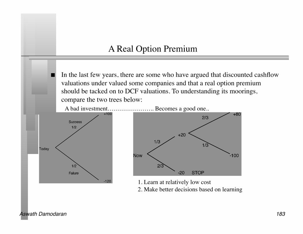
In the last few years, there are some who have argued that discounted cashflow valuations under valued some companies and that a real option premium should be tacked on to DCF valuations. To understanding its moorings, compare the two trees below:
A bad investment………………….. Becomes a good one..
1. Learn at relatively low cost 2. Make better decisions based on learning

Aswath Damodaran 184
Three Basic Questions
When is there a real option embedded in a decision or an asset? When does that real option have significant economic value? Can that value be estimated using an option pricing model?
Aswath Damodaran 185
When is there an option embedded in an action?
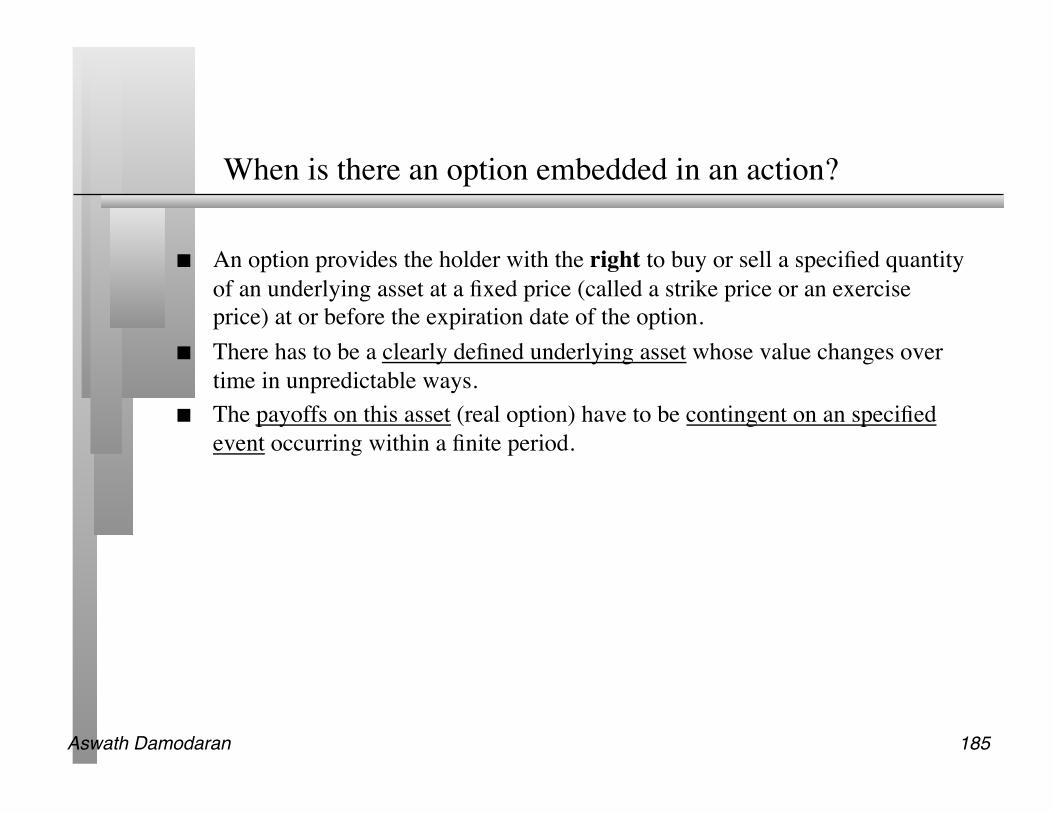
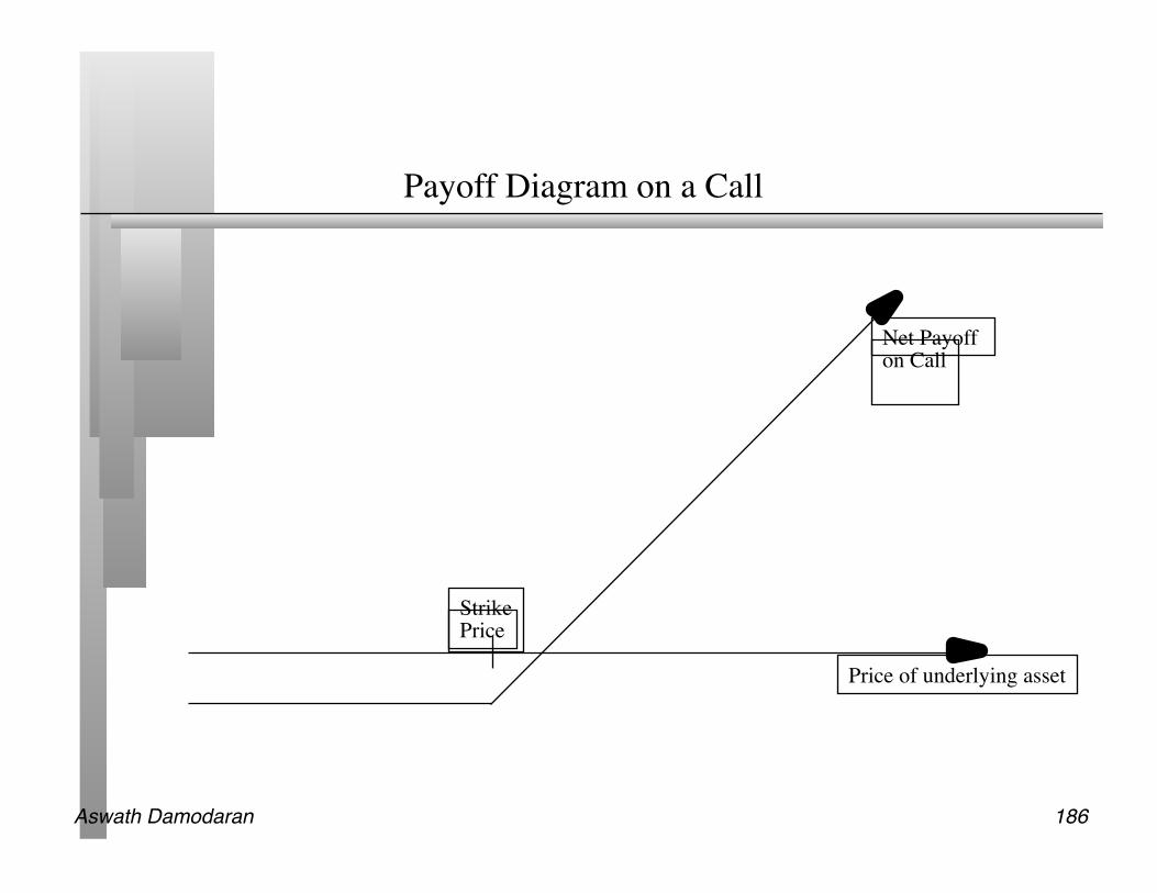
An option provides the holder with the right to buy or sell a specified quantity of an underlying asset at a fixed price (called a strike price or an exercise price) at or before the expiration date of the option.
There has to be a clearly defined underlying asset whose value changes over time in unpredictable ways.
The payoffs on this asset (real option) have to be contingent on an specified event occurring within a finite period.
Aswath Damodaran 186
Payoff Diagram on a Call
Price of underlying asset
Strike Price
Net Payoff on Call
Aswath Damodaran 187
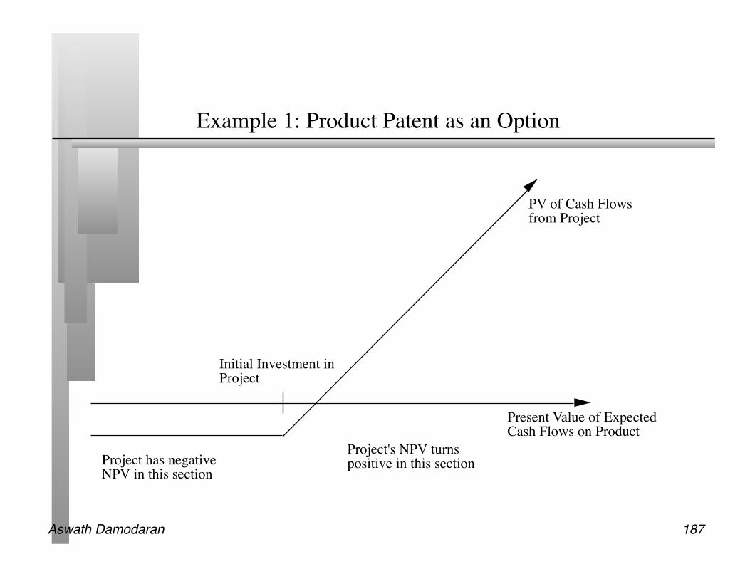
Example 1: Product Patent as an Option
Present Value of Expected Cash Flows on Product
PV of Cash Flows from Project
Initial Investment in Project
Project has negative NPV in this section
Project's NPV turns positive in this section
Aswath Damodaran 188
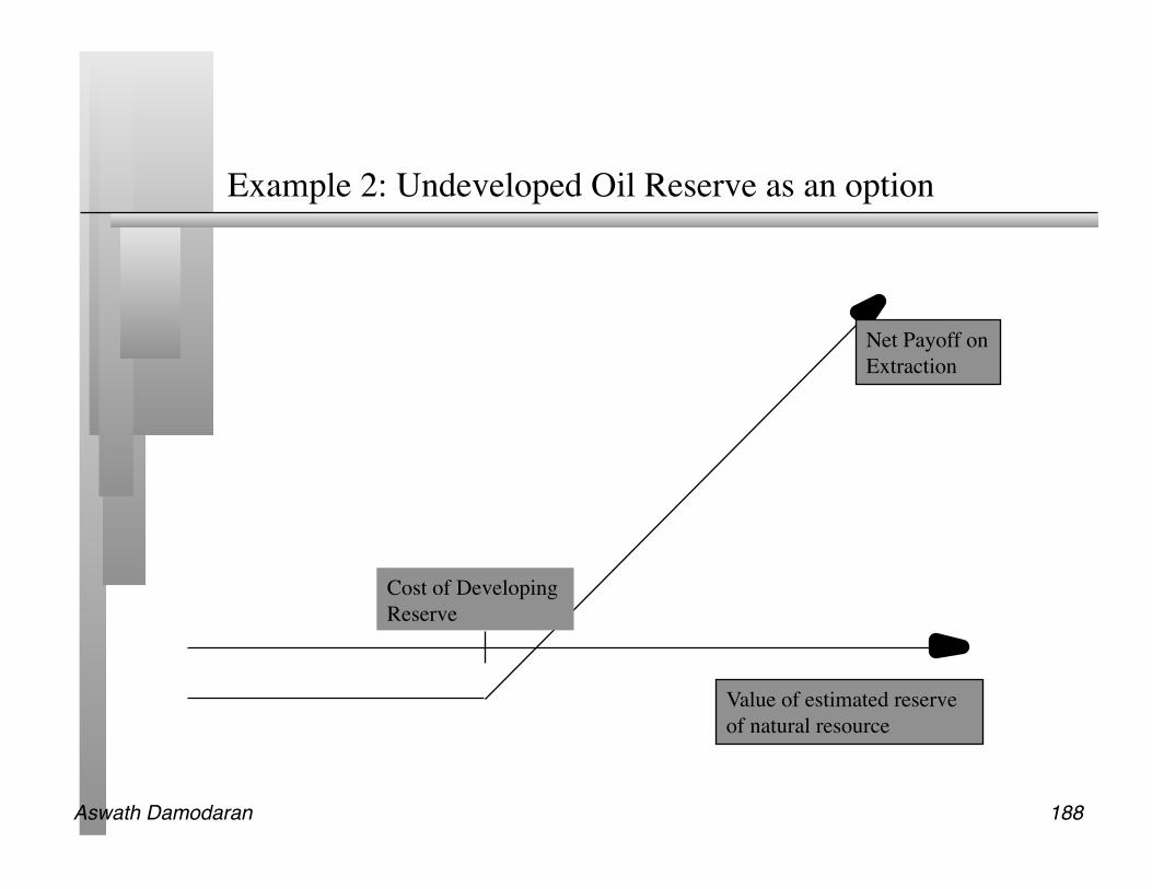
Example 2: Undeveloped Oil Reserve as an option
Value of estimated reserve of natural resource
Net Payoff on Extraction
Cost of Developing Reserve

Aswath Damodaran 189
Example 3: Expansion of existing project as an option
Present Value of Expected Cash Flows on Expansion
PV of Cash Flows from Expansion
Additional Investment to Expand
Firm will not expand in this section
Expansion becomes attractive in this section
Aswath Damodaran 190
When does the option have significant economic value?
For an option to have significant economic value, there has to be a restriction on competition in the event of the contingency. In a perfectly competitive product market, no contingency, no matter how positive, will generate positive net present value.
At the limit, real options are most valuable when you have exclusivity - you and only you can take advantage of the contingency. They become less valuable as the barriers to competition become less steep.

Aswath Damodaran 191
Exclusivity: Putting Real Options to the Test
Product Options: Patent on a drug • Patents restrict competitors from developing similar products • Patents do not restrict competitors from developing other products to treat the same
disease. Natural Resource options: An undeveloped oil reserve or gold mine.
• Natural resource reserves are limited. • It takes time and resources to develop new reserves
Growth Options: Expansion into a new product or market • Barriers may range from strong (exclusive licenses granted by the government - as
in telecom businesses) to weaker (brand name, knowledge of the market) to weakest (first mover).
Aswath Damodaran 192
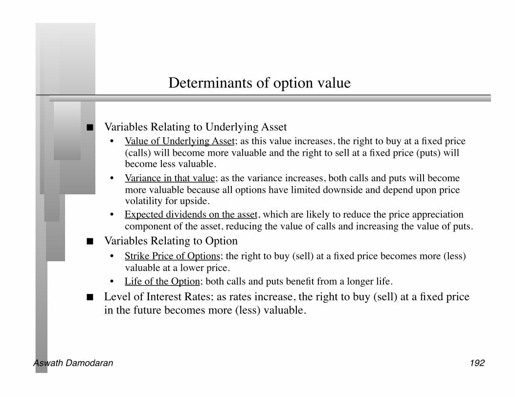
Determinants of option value
Variables Relating to Underlying Asset • Value of Underlying Asset; as this value increases, the right to buy at a fixed price
(calls) will become more valuable and the right to sell at a fixed price (puts) will become less valuable.
• Variance in that value; as the variance increases, both calls and puts will become more valuable because all options have limited downside and depend upon price volatility for upside.
• Expected dividends on the asset, which are likely to reduce the price appreciation component of the asset, reducing the value of calls and increasing the value of puts.
Variables Relating to Option • Strike Price of Options; the right to buy (sell) at a fixed price becomes more (less)
valuable at a lower price. • Life of the Option; both calls and puts benefit from a longer life.
Level of Interest Rates; as rates increase, the right to buy (sell) at a fixed price in the future becomes more (less) valuable.
Aswath Damodaran 193
The Building Blocks for Option Pricing Models: Arbitrage and Replication
The objective in creating a replicating portfolio is to use a combination of riskfree borrowing/lending and the underlying asset to create the same cashflows as the option being valued.
• Call = Borrowing + Buying Δ of the Underlying Stock • Put = Selling Short Δ on Underlying Asset + Lending • The number of shares bought or sold is called the option delta.
The principles of arbitrage then apply, and the value of the option has to be equal to the value of the replicating portfolio.
Aswath Damodaran 194
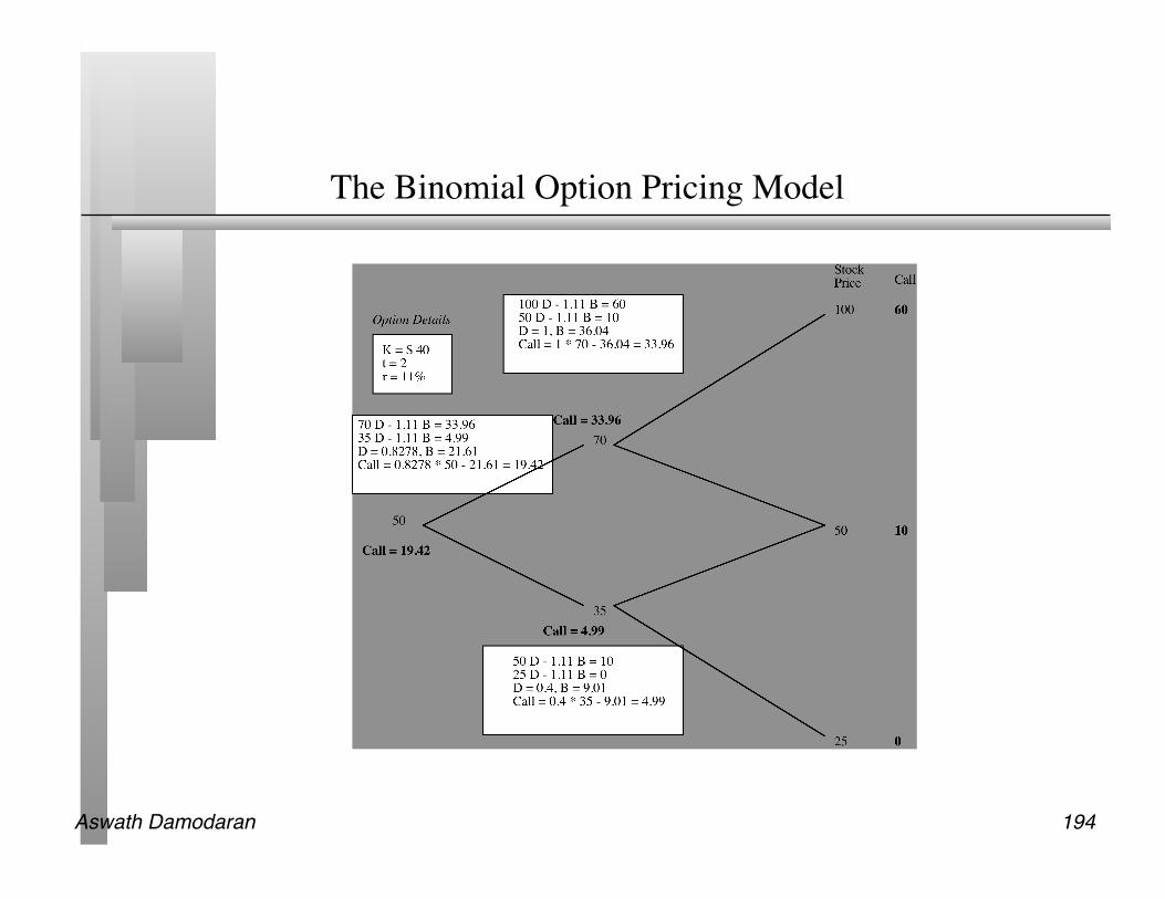
The Binomial Option Pricing Model

Aswath Damodaran 195
The Limiting Distributions….
As the time interval is shortened, the limiting distribution, as t -> 0, can take one of two forms.
• If as t -> 0, price changes become smaller, the limiting distribution is the normal distribution and the price process is a continuous one.
• If as t->0, price changes remain large, the limiting distribution is the poisson distribution, i.e., a distribution that allows for price jumps.
The Black-Scholes model applies when the limiting distribution is the normal distribution , and explicitly assumes that the price process is continuous and that there are no jumps in asset prices.
Aswath Damodaran 196
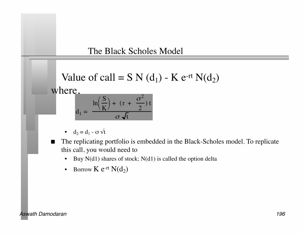
The Black Scholes Model
Value of call = S N (d1) - K e-rt N(d2) where,
• d2 = d1 - σ √t The replicating portfolio is embedded in the Black-Scholes model. To replicate
this call, you would need to • Buy N(d1) shares of stock; N(d1) is called the option delta
• Borrow K e-rt N(d2)
d1 = ln S
K
+ (r + σ
2
2) t
σ t
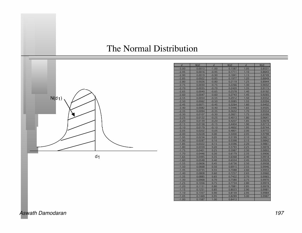
Aswath Damodaran 197
The Normal Distribution d N(d) d N(d) d N(d)
-3.00 0.0013 -1.00 0.1587 1.05 0.8531 -2.95 0.0016 -0.95 0.1711 1.10 0.8643 -2.90 0.0019 -0.90 0.1841 1.15 0.8749 -2.85 0.0022 -0.85 0.1977 1.20 0.8849 -2.80 0.0026 -0.80 0.2119 1.25 0.8944 -2.75 0.0030 -0.75 0.2266 1.30 0.9032 -2.70 0.0035 -0.70 0.2420 1.35 0.9115 -2.65 0.0040 -0.65 0.2578 1.40 0.9192 -2.60 0.0047 -0.60 0.2743 1.45 0.9265 -2.55 0.0054 -0.55 0.2912 1.50 0.9332 -2.50 0.0062 -0.50 0.3085 1.55 0.9394 -2.45 0.0071 -0.45 0.3264 1.60 0.9452 -2.40 0.0082 -0.40 0.3446 1.65 0.9505 -2.35 0.0094 -0.35 0.3632 1.70 0.9554 -2.30 0.0107 -0.30 0.3821 1.75 0.9599 -2.25 0.0122 -0.25 0.4013 1.80 0.9641 -2.20 0.0139 -0.20 0.4207 1.85 0.9678 -2.15 0.0158 -0.15 0.4404 1.90 0.9713 -2.10 0.0179 -0.10 0.4602 1.95 0.9744 -2.05 0.0202 -0.05 0.4801 2.00 0.9772 -2.00 0.0228 0.00 0.5000 2.05 0.9798 -1.95 0.0256 0.05 0.5199 2.10 0.9821 -1.90 0.0287 0.10 0.5398 2.15 0.9842 -1.85 0.0322 0.15 0.5596 2.20 0.9861 -1.80 0.0359 0.20 0.5793 2.25 0.9878 -1.75 0.0401 0.25 0.5987 2.30 0.9893 -1.70 0.0446 0.30 0.6179 2.35 0.9906 -1.65 0.0495 0.35 0.6368 2.40 0.9918 -1.60 0.0548 0.40 0.6554 2.45 0.9929 -1.55 0.0606 0.45 0.6736 2.50 0.9938 -1.50 0.0668 0.50 0.6915 2.55 0.9946 -1.45 0.0735 0.55 0.7088 2.60 0.9953 -1.40 0.0808 0.60 0.7257 2.65 0.9960 -1.35 0.0885 0.65 0.7422 2.70 0.9965 -1.30 0.0968 0.70 0.7580 2.75 0.9970 -1.25 0.1056 0.75 0.7734 2.80 0.9974 -1.20 0.1151 0.80 0.7881 2.85 0.9978 -1.15 0.1251 0.85 0.8023 2.90 0.9981 -1.10 0.1357 0.90 0.8159 2.95 0.9984 -1.05 0.1469 0.95 0.8289 3.00 0.9987 -1.00 0.1587 1.00 0.8413
Aswath Damodaran 198
When can you use option pricing models to value real options?
The notion of a replicating portfolio that drives option pricing models makes them most suited for valuing real options where
• The underlying asset is traded - this yield not only observable prices and volatility as inputs to option pricing models but allows for the possibility of creating replicating portfolios
• An active marketplace exists for the option itself. • The cost of exercising the option is known with some degree of certainty.
When option pricing models are used to value real assets, we have to accept the fact that
• The value estimates that emerge will be far more imprecise. • The value can deviate much more dramatically from market price because of the
difficulty of arbitrage.
Aswath Damodaran 199
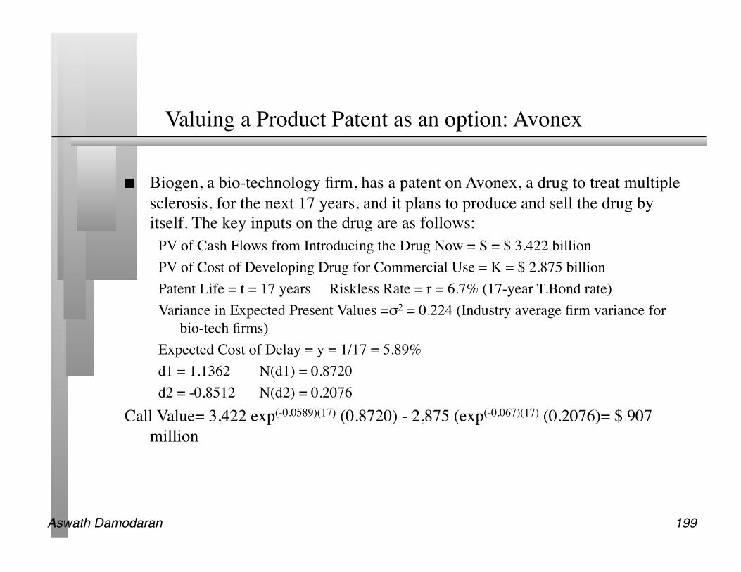
Valuing a Product Patent as an option: Avonex
Biogen, a bio-technology firm, has a patent on Avonex, a drug to treat multiple sclerosis, for the next 17 years, and it plans to produce and sell the drug by itself. The key inputs on the drug are as follows:
PV of Cash Flows from Introducing the Drug Now = S = $ 3.422 billion PV of Cost of Developing Drug for Commercial Use = K = $ 2.875 billion Patent Life = t = 17 years Riskless Rate = r = 6.7% (17-year T.Bond rate) Variance in Expected Present Values =σ2 = 0.224 (Industry average firm variance for
bio-tech firms) Expected Cost of Delay = y = 1/17 = 5.89% d1 = 1.1362 N(d1) = 0.8720 d2 = -0.8512 N(d2) = 0.2076
Call Value= 3,422 exp(-0.0589)(17) (0.8720) - 2,875 (exp(-0.067)(17) (0.2076)= $ 907 million
Aswath Damodaran 200
Valuing an Oil Reserve
Consider an offshore oil property with an estimated oil reserve of 50 million barrels of oil, where the cost of developing the reserve is $ 600 million today.
The firm has the rights to exploit this reserve for the next twenty years and the marginal value per barrel of oil is $12 per barrel currently (Price per barrel - marginal cost per barrel). There is a 2 year lag between the decision to exploit the reserve and oil extraction.
Once developed, the net production revenue each year will be 5% of the value of the reserves.
The riskless rate is 8% and the variance in ln(oil prices) is 0.03.
Aswath Damodaran 201
Valuing an oil reserve as a real option
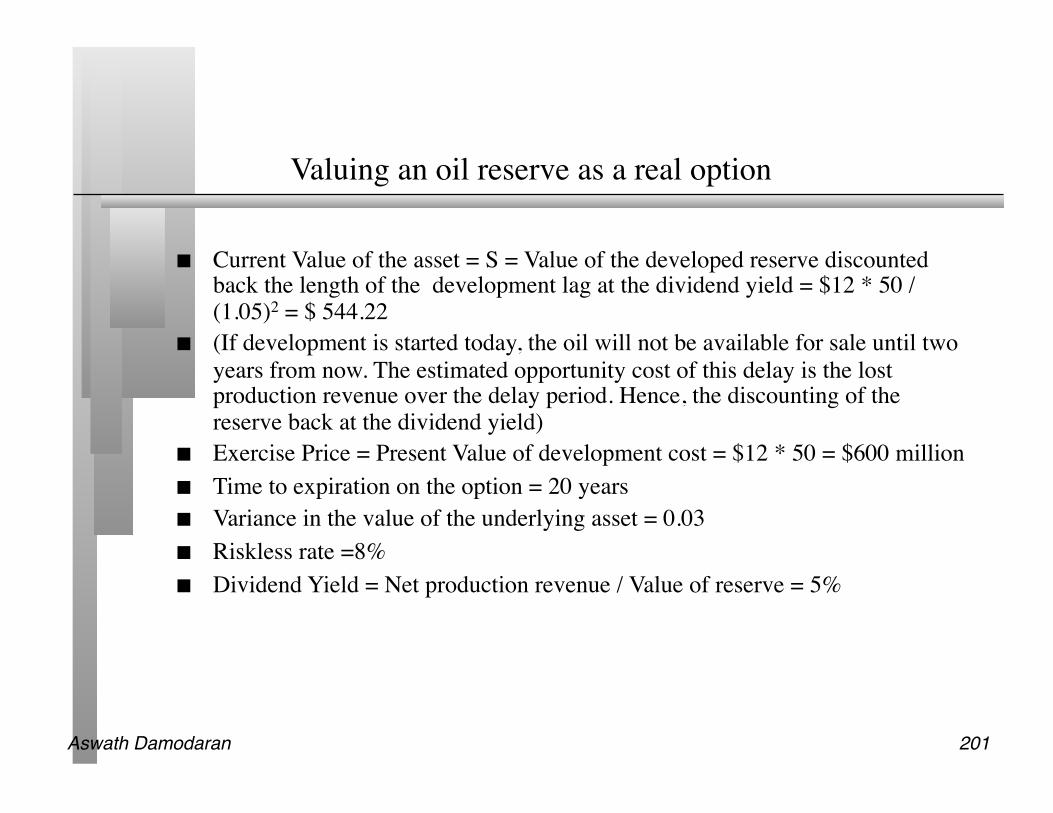
Current Value of the asset = S = Value of the developed reserve discounted back the length of the development lag at the dividend yield = $12 * 50 /(1.05)2 = $ 544.22
(If development is started today, the oil will not be available for sale until two years from now. The estimated opportunity cost of this delay is the lost production revenue over the delay period. Hence, the discounting of the reserve back at the dividend yield)
Exercise Price = Present Value of development cost = $12 * 50 = $600 million Time to expiration on the option = 20 years Variance in the value of the underlying asset = 0.03 Riskless rate =8% Dividend Yield = Net production revenue / Value of reserve = 5%
Aswath Damodaran 202
Valuing the Option
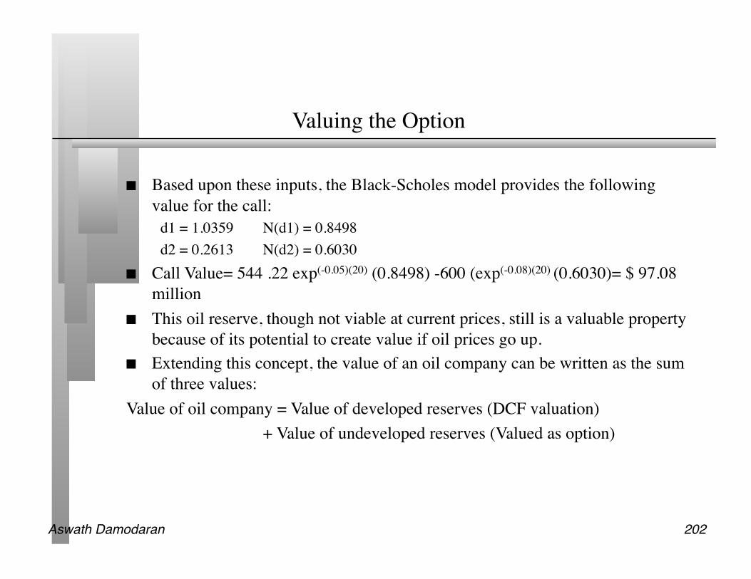
Based upon these inputs, the Black-Scholes model provides the following value for the call:
d1 = 1.0359 N(d1) = 0.8498 d2 = 0.2613 N(d2) = 0.6030
Call Value= 544 .22 exp(-0.05)(20) (0.8498) -600 (exp(-0.08)(20) (0.6030)= $ 97.08 million
This oil reserve, though not viable at current prices, still is a valuable property because of its potential to create value if oil prices go up.
Extending this concept, the value of an oil company can be written as the sum of three values:
Value of oil company = Value of developed reserves (DCF valuation) + Value of undeveloped reserves (Valued as option)
Aswath Damodaran 203
An Example of an Expansion Option
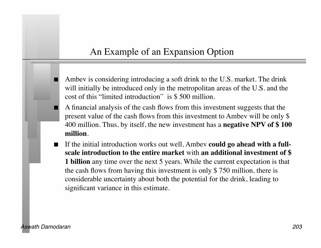
Ambev is considering introducing a soft drink to the U.S. market. The drink will initially be introduced only in the metropolitan areas of the U.S. and the cost of this “limited introduction” is $ 500 million.
A financial analysis of the cash flows from this investment suggests that the present value of the cash flows from this investment to Ambev will be only $ 400 million. Thus, by itself, the new investment has a negative NPV of $ 100 million.
If the initial introduction works out well, Ambev could go ahead with a full-scale introduction to the entire market with an additional investment of $ 1 billion any time over the next 5 years. While the current expectation is that the cash flows from having this investment is only $ 750 million, there is considerable uncertainty about both the potential for the drink, leading to significant variance in this estimate.
Aswath Damodaran 204
Valuing the Expansion Option
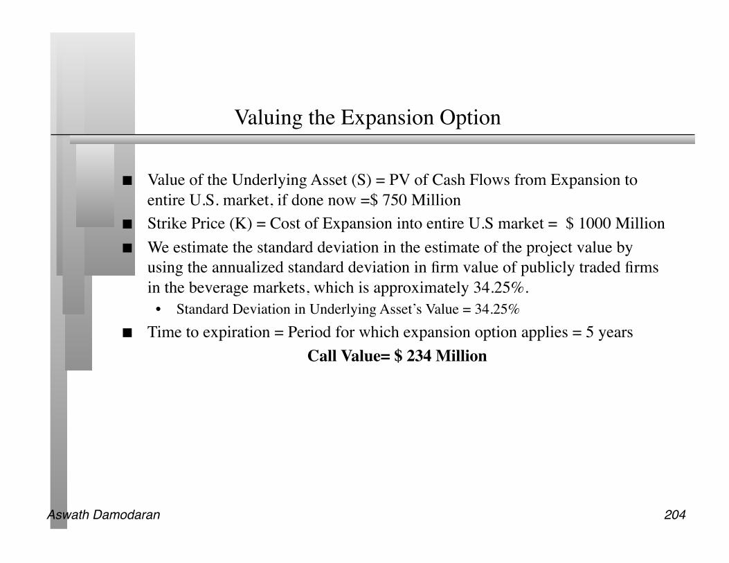
Value of the Underlying Asset (S) = PV of Cash Flows from Expansion to entire U.S. market, if done now =$ 750 Million
Strike Price (K) = Cost of Expansion into entire U.S market = $ 1000 Million We estimate the standard deviation in the estimate of the project value by
using the annualized standard deviation in firm value of publicly traded firms in the beverage markets, which is approximately 34.25%.
• Standard Deviation in Underlying Asset’s Value = 34.25% Time to expiration = Period for which expansion option applies = 5 years
Call Value= $ 234 Million
Aswath Damodaran 205
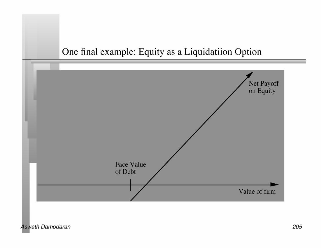
One final example: Equity as a Liquidatiion Option
Aswath Damodaran 206
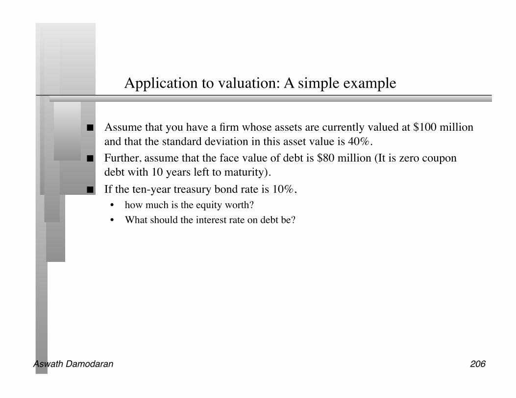
Application to valuation: A simple example
Assume that you have a firm whose assets are currently valued at $100 million and that the standard deviation in this asset value is 40%.
Further, assume that the face value of debt is $80 million (It is zero coupon debt with 10 years left to maturity).
If the ten-year treasury bond rate is 10%, • how much is the equity worth? • What should the interest rate on debt be?
Aswath Damodaran 207
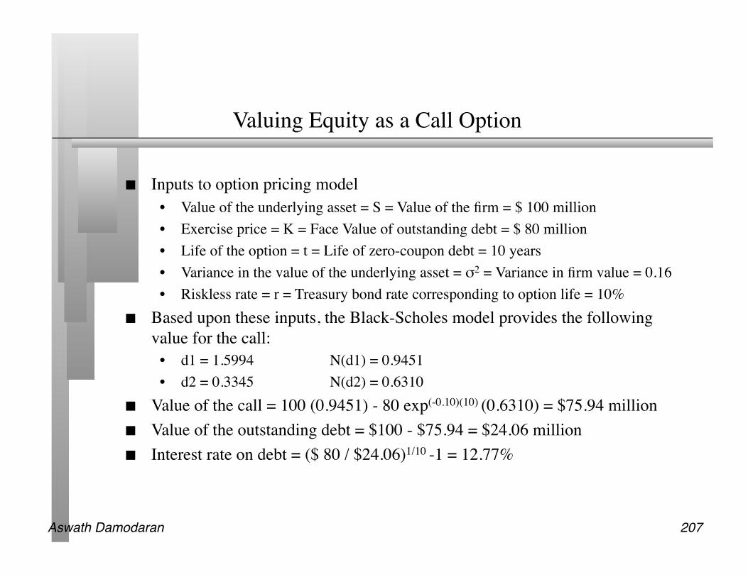
Valuing Equity as a Call Option
Inputs to option pricing model • Value of the underlying asset = S = Value of the firm = $ 100 million • Exercise price = K = Face Value of outstanding debt = $ 80 million • Life of the option = t = Life of zero-coupon debt = 10 years • Variance in the value of the underlying asset = σ2 = Variance in firm value = 0.16 • Riskless rate = r = Treasury bond rate corresponding to option life = 10%
Based upon these inputs, the Black-Scholes model provides the following value for the call:
• d1 = 1.5994 N(d1) = 0.9451 • d2 = 0.3345 N(d2) = 0.6310
Value of the call = 100 (0.9451) - 80 exp(-0.10)(10) (0.6310) = $75.94 million Value of the outstanding debt = $100 - $75.94 = $24.06 million Interest rate on debt = ($ 80 / $24.06)1/10 -1 = 12.77%
Aswath Damodaran 208
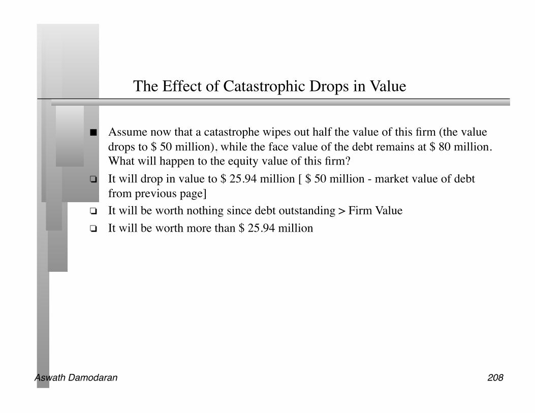
The Effect of Catastrophic Drops in Value
Assume now that a catastrophe wipes out half the value of this firm (the value drops to $ 50 million), while the face value of the debt remains at $ 80 million. What will happen to the equity value of this firm?
It will drop in value to $ 25.94 million [ $ 50 million - market value of debt from previous page]
It will be worth nothing since debt outstanding > Firm Value It will be worth more than $ 25.94 million
Aswath Damodaran 209
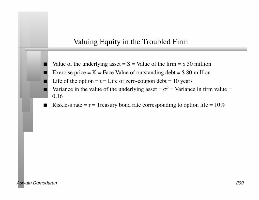
Valuing Equity in the Troubled Firm
Value of the underlying asset = S = Value of the firm = $ 50 million Exercise price = K = Face Value of outstanding debt = $ 80 million Life of the option = t = Life of zero-coupon debt = 10 years Variance in the value of the underlying asset = σ2 = Variance in firm value =
0.16 Riskless rate = r = Treasury bond rate corresponding to option life = 10%
Aswath Damodaran 210
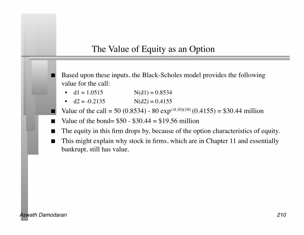
The Value of Equity as an Option
Based upon these inputs, the Black-Scholes model provides the following value for the call:
• d1 = 1.0515 N(d1) = 0.8534 • d2 = -0.2135 N(d2) = 0.4155
Value of the call = 50 (0.8534) - 80 exp(-0.10)(10) (0.4155) = $30.44 million Value of the bond= $50 - $30.44 = $19.56 million The equity in this firm drops by, because of the option characteristics of equity. This might explain why stock in firms, which are in Chapter 11 and essentially
bankrupt, still has value.

Aswath Damodaran 211
Equity value persists ..
Aswath Damodaran 212
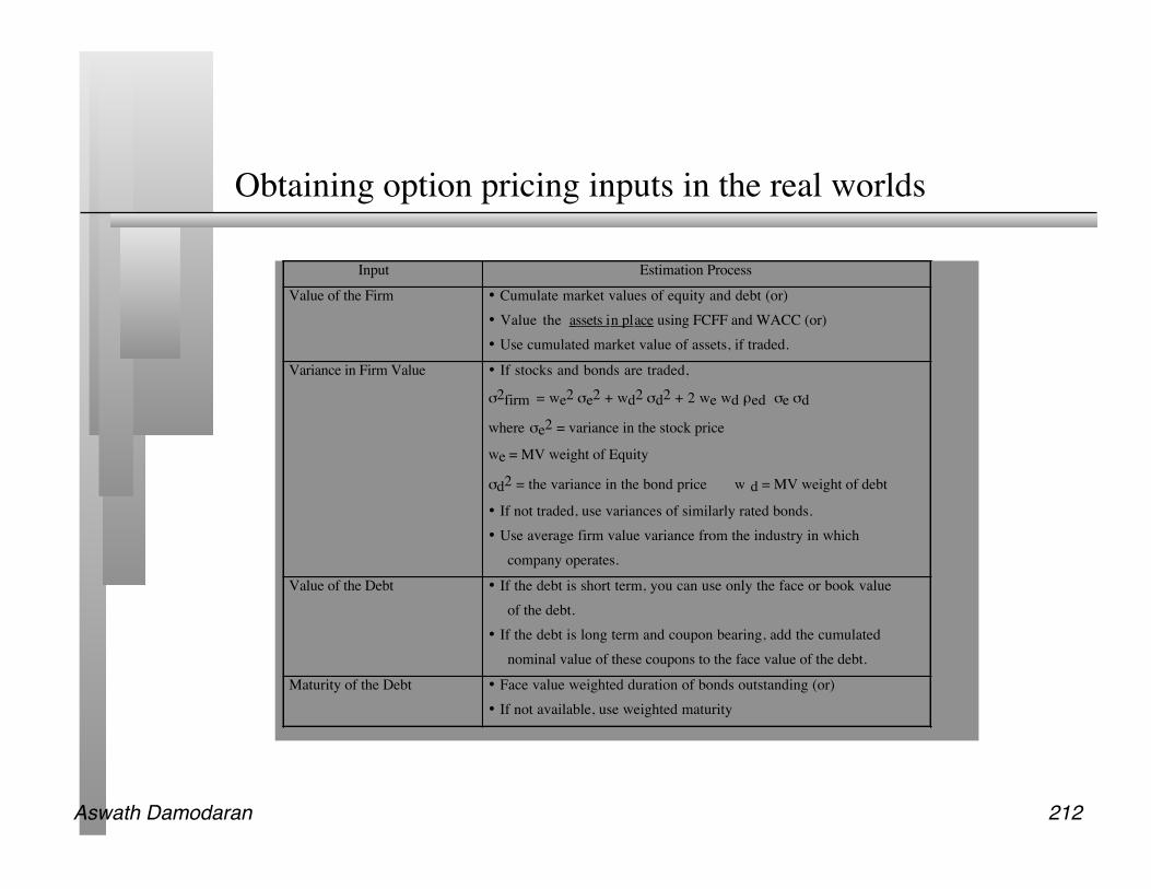
Obtaining option pricing inputs in the real worlds
Input Estimation Process
Value of the Firm • Cumulate market values of equity and debt (or)• Value the assets in place using FCFF and WACC (or)• Use cumulated market value of assets, if traded.
Variance in Firm Value • If stocks and bonds are traded,
σ2firm = we2 σe2 + wd2 σd2 + 2 we wd ρed σe σd
where σe2 = variance in the stock price
we = MV weight of Equity
σd2 = the variance in the bond price w d = MV weight of debt
• If not traded, use variances of similarly rated bonds.• Use average firm value variance from the industry in which
company operates.
Value of the Debt • If the debt is short term, you can use only the face or book valueof the debt.
• If the debt is long term and coupon bearing, add the cumulatednominal value of these coupons to the face value of the debt.
Maturity of the Debt • Face value weighted duration of bonds outstanding (or)• If not available, use weighted maturity
Aswath Damodaran 213
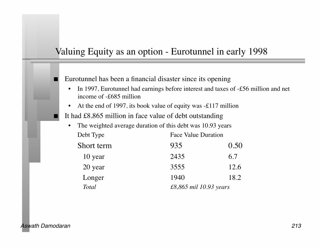
Valuing Equity as an option - Eurotunnel in early 1998
Eurotunnel has been a financial disaster since its opening • In 1997, Eurotunnel had earnings before interest and taxes of -£56 million and net
income of -£685 million • At the end of 1997, its book value of equity was -£117 million
It had £8,865 million in face value of debt outstanding • The weighted average duration of this debt was 10.93 years Debt Type Face Value Duration
Short term 935 0.50 10 year 2435 6.7 20 year 3555 12.6 Longer 1940 18.2
Total £8,865 mil 10.93 years

Aswath Damodaran 214
The Basic DCF Valuation
The value of the firm estimated using projected cashflows to the firm, discounted at the weighted average cost of capital was £2,312 million.
This was based upon the following assumptions – • Revenues will grow 5% a year in perpetuity. • The COGS which is currently 85% of revenues will drop to 65% of revenues in yr
5 and stay at that level. • Capital spending and depreciation will grow 5% a year in perpetuity. • There are no working capital requirements. • The debt ratio, which is currently 95.35%, will drop to 70% after year 5. The cost
of debt is 10% in high growth period and 8% after that. • The beta for the stock will be 1.10 for the next five years, and drop to 0.8 after the
next 5 years. • The long term bond rate is 6%.

Aswath Damodaran 215
Other Inputs
The stock has been traded on the London Exchange, and the annualized std deviation based upon ln (prices) is 41%.
There are Eurotunnel bonds, that have been traded; the annualized std deviation in ln(price) for the bonds is 17%.
• The correlation between stock price and bond price changes has been 0.5. The proportion of debt in the capital structure during the period (1992-1996) was 85%.
• Annualized variance in firm value = (0.15)2 (0.41)2 + (0.85)2 (0.17)2 + 2 (0.15) (0.85)(0.5)(0.41)(0.17)= 0.0335
The 15-year bond rate is 6%. (I used a bond with a duration of roughly 11 years to match the life of my option)
Aswath Damodaran 216
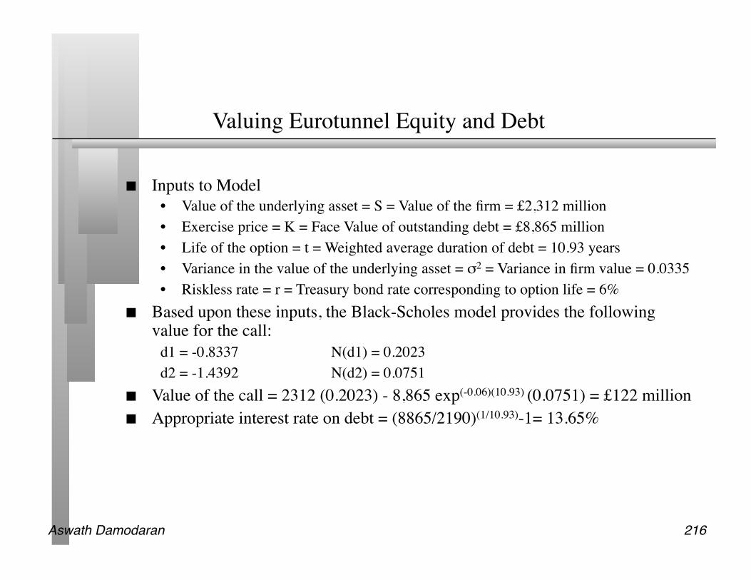
Valuing Eurotunnel Equity and Debt
Inputs to Model • Value of the underlying asset = S = Value of the firm = £2,312 million • Exercise price = K = Face Value of outstanding debt = £8,865 million • Life of the option = t = Weighted average duration of debt = 10.93 years • Variance in the value of the underlying asset = σ2 = Variance in firm value = 0.0335 • Riskless rate = r = Treasury bond rate corresponding to option life = 6%
Based upon these inputs, the Black-Scholes model provides the following value for the call:
d1 = -0.8337 N(d1) = 0.2023 d2 = -1.4392 N(d2) = 0.0751
Value of the call = 2312 (0.2023) - 8,865 exp(-0.06)(10.93) (0.0751) = £122 million Appropriate interest rate on debt = (8865/2190)(1/10.93)-1= 13.65%
Aswath Damodaran 217
Back to Lemmings...