Embed Size (px)
Citation preview
Real Time Autotuning for MapReduce onHadoop/YARN
by
Maria Pospelova, B.Sc.
A thesis submitted to the
Faculty of Graduate and Postdoctoral Affairs
in partial fulfillment of the requirements for the degree of
Master of Computer Science (Accelerated) with Data Science
Specialization
Ottawa-Carleton Institute of Computer Science
Department of Computer Science
Carleton University
Ottawa, Ontario
July, 2015
c©Copyright
Maria Pospelova, 2015
The undersigned hereby recommends to the
Faculty of Graduate and Postdoctoral Affairs
acceptance of the thesis
Real Time Autotuning for MapReduce on Hadoop/YARN
submitted by Maria Pospelova, B.Sc.
in partial fulfillment of the requirements for the degree of
Master of Computer Science (Accelerated) with Data Science
Specialization
Professor Herna L Viktor, Ph.D, External Examiner
Professor Michel Barbeau, Ph.D, Examiner
Professor Frank Dehne, Ph.D, Thesis Supervisor
Professor Anil Somayaji, Ph.D, Chair,Department of Computer Science
Ottawa-Carleton Institute of Computer Science
Department of Computer Science
Carleton University
July, 2015
ii
Abstract
Humanity entered the Big Data era passing through the zettabite mark at an ex-
ponential rate in just a few years, which made Big Data processing issues a reality
for a wide range of business and academic applications. The Apache Hadoop is the
most popular Big Data processing framework with the current market share of $3
billion expected to increase to $50 billion by the end of the decade; however, Hadoop
deployment expansion does not proceed at the predicted rate.
One of the obstacles for further popularization of Hadoop is that performance
is highly dependent on chosen settings. A nontrivial tuning process requires time
and highly qualified human resources. Therefore, an automatic tuner is a desirable
solution. Existent off-line tuning approaches require multiple repetitive executions of
the job in order to find optimal tuning settings and, hence, are not applicable to use
in most cases.
The presented work introduces a novel real time autotuning approach. The re-
source management parameters are tuned between execution waves by a modular au-
totuner connected to Hadoop architecture through YARN. The developed autotuner
effectively intercepts a resource request, modifies it according to a tuning algorithm
and passes it to YARN Scheduler. Such an approach not only carries high practical
and theoretical value, but also opens a new horizon in the Hadoop/YARN automatic
tuning development.
iii

This thesis is dedicated to my husband, Pino Guerra, and to my children, Matteo
and Isabella. Thank you for your love, patience, and numerous sacrifices that you
have made throughout my academic career. This thesis and the pursuit of my goals
would not have been possible without your support.
iv
Acknowledgments
Foremost, I would like to express my special appreciation and my sincere gratitude
to my advisor Professor Dr. Frank Dehne. You have been a tremendous mentor. I
would like to thank you for encouraging my research and for allowing me to grow
as a research scientist. Your advice on both research and on my career have been
priceless.
I would also like to thank Professor Dr. Michel Barbeau, Professor Dr. Anil
Somayaji, Professor Dr. Herna Viktor for serving as my committee members.
Furthermore I would like to thank my collaborator, Mikhail Genkin, for introduc-
ing me to the topic and sharing his invaluable experience and his talents. It would
not have been possible without his crucial help.
My gratitude also goes out to the Parallel Computing and Data Science Research
Lab members. I especially want to thank Dr. Sylvain Pitre and Andrew Schoenrock,
who provided me with advice and support at times of critical need.
I take this opportunity to express gratitude to all of the School of Computer
Science and the new Institute for Data Science faculty members for their help and
support.
v
Table of Contents
Abstract iii
Acknowledgments v
Table of Contents vi
List of Tables x
List of Figures xi
1 Introduction 1
1.1 Data Science and Big Data Computing . . . . . . . . . . . . . . . . . 1
1.2 MapReduce . . . . . . . . . . . . . . . . . . . . . . . . . . . . . . . . 2
1.3 Hadoop . . . . . . . . . . . . . . . . . . . . . . . . . . . . . . . . . . 3
1.4 Auto-tuning Hadoop . . . . . . . . . . . . . . . . . . . . . . . . . . . 4
1.5 Thesis Motivation . . . . . . . . . . . . . . . . . . . . . . . . . . . . . 5
1.6 Thesis Contributions . . . . . . . . . . . . . . . . . . . . . . . . . . . 5
1.7 Thesis Organization . . . . . . . . . . . . . . . . . . . . . . . . . . . . 5
2 MapReduce 6
2.1 General Concept . . . . . . . . . . . . . . . . . . . . . . . . . . . . . 6
2.2 MapReduce Implementations . . . . . . . . . . . . . . . . . . . . . . 6
2.3 Specifics of the Apache Hadoop . . . . . . . . . . . . . . . . . . . . . 8
3 State of the Art 10
4 Autotuning Algorithms 14
4.1 Simulated Annealing . . . . . . . . . . . . . . . . . . . . . . . . . . . 14
4.2 Genetic Algorithm . . . . . . . . . . . . . . . . . . . . . . . . . . . . 16
vi

4.3 Hill Climbing . . . . . . . . . . . . . . . . . . . . . . . . . . . . . . . 18
5 Hadoop Source Code 20
5.1 Overall Architecture . . . . . . . . . . . . . . . . . . . . . . . . . . . 20
5.1.1 Original Apache Hadoop MapReduce . . . . . . . . . . . . . . 21
5.1.2 Apache Hadoop Yet-Another-Resource-Negotiator (YARN) . . 22
5.2 Hadoop on YARN . . . . . . . . . . . . . . . . . . . . . . . . . . . . . 23
5.2.1 YARN Application Execution Overview . . . . . . . . . . . . 24
5.2.2 MapReduce Job Execution Overview . . . . . . . . . . . . . . 24
5.3 Detailed Exploration of the Current Implementation of the Most Rel-
evant Packages . . . . . . . . . . . . . . . . . . . . . . . . . . . . . . 26
5.3.1 Resource Manager . . . . . . . . . . . . . . . . . . . . . . . . 26
5.3.2 Scheduler Related Components . . . . . . . . . . . . . . . . . 27
5.3.3 Client Interfacing Components . . . . . . . . . . . . . . . . . 27
5.3.4 Connecting to the Nodes Components . . . . . . . . . . . . . 27
5.3.5 Application Masters’ interacting components . . . . . . . . . . 28
5.4 Application Master . . . . . . . . . . . . . . . . . . . . . . . . . . . . 29
5.5 YARN Schedulers . . . . . . . . . . . . . . . . . . . . . . . . . . . . . 30
5.5.1 The FIFO Scheduler . . . . . . . . . . . . . . . . . . . . . . . 30
5.5.2 The Capacity Scheduler . . . . . . . . . . . . . . . . . . . . . 31
5.5.3 The Fair Scheduler . . . . . . . . . . . . . . . . . . . . . . . . 31
5.6 Tunable Hadoop Parameters . . . . . . . . . . . . . . . . . . . . . . . 31
6 Autotuner Implementation 35
6.1 Overview of the Autotuner Placement Within the Hadoop . . . . . . 35
6.2 Autotuner Implementation Details . . . . . . . . . . . . . . . . . . . 37
6.2.1 Autotuner Classes . . . . . . . . . . . . . . . . . . . . . . . . 37
6.2.2 Autotuner Waves . . . . . . . . . . . . . . . . . . . . . . . . . 38
6.2.3 Execution order of the Autotuner . . . . . . . . . . . . . . . . 39
6.2.4 Explorer . . . . . . . . . . . . . . . . . . . . . . . . . . . . . . 40
7 Results 41
7.1 Experimental Design . . . . . . . . . . . . . . . . . . . . . . . . . . . 41
7.1.1 Testing Cluster Configuration and Hardware . . . . . . . . . . 41
7.1.2 Hadoop Cluster Settings . . . . . . . . . . . . . . . . . . . . . 42
vii
7.1.3 Development environment set up with MiniYARNcluster on
Eclipse development environment . . . . . . . . . . . . . . . . 42
7.1.4 Benchmarks . . . . . . . . . . . . . . . . . . . . . . . . . . . . 44
7.1.5 TeraSort Benchmark . . . . . . . . . . . . . . . . . . . . . . . 44
7.1.6 TPCx-HS Benchmark . . . . . . . . . . . . . . . . . . . . . . . 46
7.1.7 NMON . . . . . . . . . . . . . . . . . . . . . . . . . . . . . . . 47
7.2 Parameter Space Exploration . . . . . . . . . . . . . . . . . . . . . . 47
7.3 Default Baseline . . . . . . . . . . . . . . . . . . . . . . . . . . . . . . 48
7.3.1 TeraSort . . . . . . . . . . . . . . . . . . . . . . . . . . . . . . 48
7.3.2 TCPx-HS . . . . . . . . . . . . . . . . . . . . . . . . . . . . . 49
7.4 Preliminary Autotuner Results . . . . . . . . . . . . . . . . . . . . . . 52
7.4.1 TeraSort . . . . . . . . . . . . . . . . . . . . . . . . . . . . . . 52
7.4.2 TPCx-HS . . . . . . . . . . . . . . . . . . . . . . . . . . . . . 53
7.5 Explorer . . . . . . . . . . . . . . . . . . . . . . . . . . . . . . . . . . 53
7.5.1 Explorer with 30-second Autotuner waves on memory and vCores 53
7.5.2 Explorer with 20-minute Autotuner waves on memory . . . . . 54
8 Discussion 57
8.1 Innovation Concept. Real-Time Autotuning . . . . . . . . . . . . . . 57
8.1.1 Rational for real-time Hadoop YARN autotuning . . . . . . . 57
8.1.2 Autotuner Design Requirements . . . . . . . . . . . . . . . . . 58
8.2 Design Decisions Motivation . . . . . . . . . . . . . . . . . . . . . . . 58
8.3 Result Evaluation . . . . . . . . . . . . . . . . . . . . . . . . . . . . . 62
8.3.1 Comparison of the Preliminary Autotuner Runs with Default
and RoT Testings . . . . . . . . . . . . . . . . . . . . . . . . . 62
8.3.2 Explanation of the Results Obtained by Preliminary Autotuner
Testing and Explorer Execution . . . . . . . . . . . . . . . . . 62
8.3.3 Strength of the Current Autotuner Design . . . . . . . . . . . 64
8.3.4 Weakness of the Current Autotuner Design and Ideas for Im-
provement . . . . . . . . . . . . . . . . . . . . . . . . . . . . . 65
9 Summary 67
9.1 Overview of the Results . . . . . . . . . . . . . . . . . . . . . . . . . 67
9.2 Future Development . . . . . . . . . . . . . . . . . . . . . . . . . . . 68
viii

List of References 70
Appendix A The List of Imports for a MiniYARNCluster 73
ix
List of Tables
5.1 The Default and Rules of Thumb (RoT) settings for Hadoop Parameters 33
7.1 Completion Times for TeraSort on 100 GB Data with Different Values
of mapreduce. ∗ .memory.mb Parameters with Calculated Standard
Deviation . . . . . . . . . . . . . . . . . . . . . . . . . . . . . . . . . 48
7.2 TPCx-HS Default Baseline Tests Results . . . . . . . . . . . . . . . . 52
7.3 TeraSort on 100GB of data with Autotuner Empowered Hadoop with
Hill Climbing Algorithm Tests Results . . . . . . . . . . . . . . . . . 52
7.4 TPCx-HS with Autotuner Empowered Hadoop with Hill Climbing Al-
gorithm Tests Results . . . . . . . . . . . . . . . . . . . . . . . . . . 53
x
List of Figures
2.1 MapReduce Concept . . . . . . . . . . . . . . . . . . . . . . . . . . . 7
5.1 Original Apache Hadoop MapReduce Architecture . . . . . . . . . . . 21
5.2 Apache Hadoop Yet-Another-Resource-Negotiator (YARN) Architecture 22
5.3 Apache Hadoop on YARN Structure . . . . . . . . . . . . . . . . . . 24
5.4 MapReduce Jod Run on Apache Hadoop on YARN . . . . . . . . . . 26
6.1 Hadoop YARN Resource Requesting Scheme . . . . . . . . . . . . . . 36
6.2 Autotuner Placement in Hadoop YARN . . . . . . . . . . . . . . . . 37
6.3 Autotuner Waves . . . . . . . . . . . . . . . . . . . . . . . . . . . . . 39
7.1 TPCx-HS Execution Phases . . . . . . . . . . . . . . . . . . . . . . . 46
7.2 Graph of Completion Times for TeraSort on 100GB Data with Different
Values of mapreduce. ∗ .memory.mb Parameters . . . . . . . . . . . . 49
7.3 NMON Analyzer results for 1TB Terasort test with default parameters.
(A) Total CPU Utilization, (B) CPU Utilization per CPU, (C) Disk
I/O, (D) Network I/O, (E) Network Packets. . . . . . . . . . . . . . . 50
7.4 NMON Analyzer results for 1TB Terasort test with default parameters.
(A) Total CPU Utilization, (B) CPU Utilization per CPU, (C) Disk
I/O, (D) Network I/O, (E) Network Packets. . . . . . . . . . . . . . . 51
7.5 Hadoop empowered by the autotuner with Explorer algorithm with
30-second autotuner waves on memory and vCores . . . . . . . . . . . 54
7.6 Hadoop empowered by the autotuner with Explorer algorithm with
with 20-minute autotuner waves on memory for the 1 TB TeraSort . 55
7.7 Hadoop empowered by the autotuner with Explorer algorithm with 20-
minute autotuner waves on memory for the 1 TB TeraSort (the later
20%) . . . . . . . . . . . . . . . . . . . . . . . . . . . . . . . . . . . 55
7.8 Hadoop empowered by the autotuner with Explorer algorithm with
Explorer algorithm with 20-minute autotuner waves on memory for
the 2 TB TeraSort . . . . . . . . . . . . . . . . . . . . . . . . . . . . 56
xi

7.9 Hadoop empowered by the autotuner with Explorer algorithm with
Explorer algorithm with 20-minute autotuner waves on memory for
the 2 TB TeraSort (the later 20%) . . . . . . . . . . . . . . . . . . . 56
8.1 Comparison of the trend-lines: (A) Complete Terasort execution times,
(B) Average container completion time per the autotuner wave during
1TB Terasort, (C) Average container completion time per the auto-
tuner wave during 2TB Terasort . . . . . . . . . . . . . . . . . . . . . 61
xii

Chapter 1
Introduction
1.1 Data Science and Big Data Computing
The estimated size of all digital data approaches 8 zettabytes, and this number is
projected to continuously increase at an exponential rate. Hence, dealing with the
Big Data processing problem is inescapable. Moreover, just a few years ago, this was a
problem of the industry giants, such as Google and Amazon, now much greater share
of business and academic projects must find a solution. The Big Data processing is
a very new, extremely challenging and demanding area of research. Because of such
circumstances, not only does a commonly accepted solution not exist, but also the
definition of the term, Big Data, itself, is constantly challenged.
The Big Data term was added to the Oxford English Dictionary just two years
ago [1], yet the term has been circulating in technical circles since the mid 90s. The
most common definition describes Big Data as the high volume, high velocity, and
high variety digital information collection. This definition is also known as ”three V’s”
definition, and was originally given by Doug Laney in 2001 [2]. Yet many reputable
experts disagree with this definition and propose their own. Nevertheless, most of the
professionals agree that extremely challenging processing is one of the most prominent
characteristics of Big Data.
In order to harvest useful information from the Big Data, the data science field
emerged. Data scientists role requires domain knowledge, a mathematical and statis-
tical base along with technical programming skills. However, most of all, it requires a
curious, creative state of mind, which prompts data scientists to explore the data in
many different ways: testing out various hypotheses in a search of interesting patterns
and correlations, and translating solutions from one domain to another. For instance,
1
CHAPTER 1. INTRODUCTION 2
Davenport and Patil brought up an example of a data scientist who not only found
similarity between a DNA sequencing problem and a fraud investigation they were
working on, but also successfully applied an existing solution to the new domain [3].
Moreover, the experimental nature of data science requires a quick response to a wide
variety of data processing tasks.
1.2 MapReduce
Before the popularization by Dean and colleagues, in 2004, [4], as a panacea for all Big
Data problems, the MapReduce technique was already known among distributed and
parallel computing professionals. However, Google’s publication certainly brought
the technique to light for the rest by adding a new spin and causing its popularity to
spread like wildfire.
MapReduce is a computational model based on functional programming concepts
of list processing. One of the key concepts of functional programming, data im-
mutability, supports reliable and efficient distributed data processing without costly
and fault-prone current state synchronization issues. Each task does not modify input
key-value pairs, but produces new ones with modified values, which are forwarded by
the Hadoop system into the next phase of execution. A MapReduce program is com-
posed of two list-processing idioms, which are exposed to the user: map, and reduce.
These terms are also not new and had been previously used in other list-processing
languages such as LISP, Scheme, and ML.
The first phase, mapping, executes Mapper, a function, which transforms the ele-
ments of the input list to output data elements, acting on each element individually.
Next, the shuffling phase, which is transparent to the user, rearranges output pro-
duced by Mapper. Shuffle process results in all data pairs with the same key being
localized together and assigned to the same reducer. Then, in the reduce phase,
Reducer, a function which aggregate values together, receives an iterator for the pro-
duced list and combines these values together, returning an output value.
Since its introduction, MapReduce gained a strong position for Big Data process-
ing applications of various natures in both industry and academia. The most popular
MapReduce implementation is the Apache Hadoop.
CHAPTER 1. INTRODUCTION 3
1.3 Hadoop
Initiated by Doug Cutting and Mike Cafarella, an open-source search engine, Nutch,
was inspired by two famous Google papers [5,6]. Later in 2006, when Cutting started
his work at Yahoo, Hadoop was given its name. Moreover, the original Hadoop run-
ning cluster, which was built as proof of a concept for a new search engine, was noticed
by Yahoo’s data scientists for its surprisingly good performance. The success of Ya-
hoo’s search relevance or Yahoo’s advertising revenue analytics built on Hadoop led
to the ”behind every click” keystone position at Yahoo. Together, Yahoo developers
and open-source contributors brought Hadoop to the solid state, which allowed it to
be chosen as a primary MapReduce education framework. A cluster of 2000 Hadoop
nodes was sponsored by IBM, Google and the National Science Foundation. Later,
Cloudera and Hortonworks, commercial Hadoop companies, played an important role
in increasing the popularity and furthering the business deployment of the Hadoop.
Some of the advantages of an open-source project is its ability to react quickly
to new industry demands, and incorporate innovative technologies. The evolution
of Hadoop, since its creation, is tremendous. Nevertheless, the recent transition to
YARN-based architecture could be considered the most significant framework up-
grade since Hadoop’s creation. YARN (Yet Another Resource Negotiator) expanded
the Hadoop programming model from strictly MapReduce to a variety of process-
ing engines. YARN architecture for resource management provides more consistent
performance, better governance of the data across Hadoop clusters, and improved
security.
The new resource management system built upon the container concept. Con-
tainers are resource partition abstractions of the specified size, which are used as
a currency to negotiate the distribution of the Hadoop cluster resources among the
applications. The Application Master requests a specific number of containers with
a certain size of the memory and a number of virtual cores. The Resource Man-
ager collects the requests and passes them to a YARN scheduler. The scheduler
distributes currently available resources by partially satisfying incoming requests,
as total of requested resources is usually much greater than the total of currently
available resources. This action is repeated periodically, on each heartbeat. Simulta-
neously allocated containers form a wave. Considering allocation happens on almost
every heartbeat, by default, the heartbeats emitted every minute number of waves
per application is significant. The size of memory and the number of virtual cores
CHAPTER 1. INTRODUCTION 4
per container are set in configuration file by the user, and are static throughout the
job execution. Moreover, they affect job completion time significantly.
Since its creation, Hadoop has come a long way. In 2011, it was proclaimed the
most important innovation, surpassing Apple’s iPad, and receiving the top prize of
the MediaGuardian Innovation Award. The future is also bright; IDC predicts that
Hadoop-MapReduce ecosystem will be worth $813 million by the next year [7]. Fur-
thermore, the experts suggest that its actual economical impact will be significantly
greater.
1.4 Auto-tuning Hadoop
Tuning a Hadoop MapReduce job is a nontrivial task. Hadoop exposes over two
hundred parameters, many of which have a severe impact on job performance. A
poorly configured job can result in extremely slow execution times or even failure.
Currently, the industry standard is manual tuning, which requires iterative repetition
of the job execution with adjustment of xml configuration files by highly qualified
professionals. Such professionals are in high demand. Moreover, as the range of
Hadoop users expands, many of the users cannot obtain such employees due to a
shortage in the availability or resources.
The growing importance of Apache Hadoop, the severity of the impacts of pa-
rameter selection, along with the limitation of resources, has led to vivid interest in
the research community. A number of studies explored the variety of off-line tun-
ing. Some of them were based on a statistical model with the incorporation of ”rule
of thumb” knowledge, such as the Starfish project [8, 9]. Another group of projects
favoured an algorithmic approach such as the Gunther [10] and Panda [11] projects.
Many of them achieved impressive results in the improvement of job completion time.
Unfortunately, such results could be translated into a practical value only for use cases
in which the same job is repetitively executed on the same size data, as any changes
in the job or the size of data will require adjustments in tunable parameters. There-
fore, for many data science use cases, repetitive iteration of the single job by off-line
autotuner not only does not speed up the process but also makes job completion time
magnitudes slower.
CHAPTER 1. INTRODUCTION 5
1.5 Thesis Motivation
The answer to the stated problem is a real time Hadoop autotuning process, which
allows the optimization of cluster deployment and completion time of a MapReduce
job executed on Hadoop/YARN during a single run. A real time autotuning solution
will extend to all Hadoop use cases including repetitively and single time executed
MapReduce jobs. Moreover, a real time autotuning would solve the problem with
human recourse shortage, opening effective Hadoop/YARN deployment to a much
wider sector of users.
1.6 Thesis Contributions
The work presented in the thesis lays a strong base for the complete real time auto-
tuning Hadoop/YARN solution and provides proof of a concept that such tuning is
possible through a working autotuner implementation. The presented autotuner ad-
justs container parameters (size of memory and number of virtual cores) in real time,
during a single job execution. Moreover, an effective cost evaluating function, which
estimates total job completion time based on information collected in a fraction of a
total job, was developed. Furthermore, the test results confirmed the effectiveness of
the cost function, along with the autotuner architecture and its Hadoop/YARN inte-
gration scheme. Hence, the thesis work lays a solid foundation for the development
of an effective real time Hadoop/YARN autotuning solution.
1.7 Thesis Organization
Chapter 2 introduces the main concepts of MapReduce and its implementations.
Chapter 3 summarizes state of the art of autotuning research for Hadoop MapReduce
jobs. Chapter 4 briefly introduces the commonly used automatic tuning algorithms
for Hadoop, which were considered for the current autotuner. Chapter 5 reflects
the main points and concepts of Apache Hadoop Architecture based on a detailed
study of Hadoop source code and documentation. Chapter 6 describes the developed
real time autotuner implementation. Chapter 7 describes experimental design and
collected results. Chapter 8 presents the analysis of the observed results. Chapter 9
summarizes findings and outlines prospective steps for future development.
Chapter 2
MapReduce
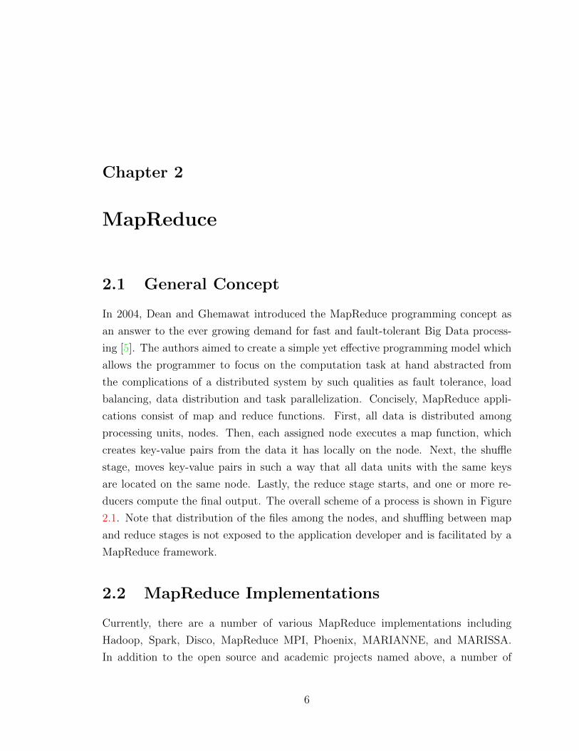
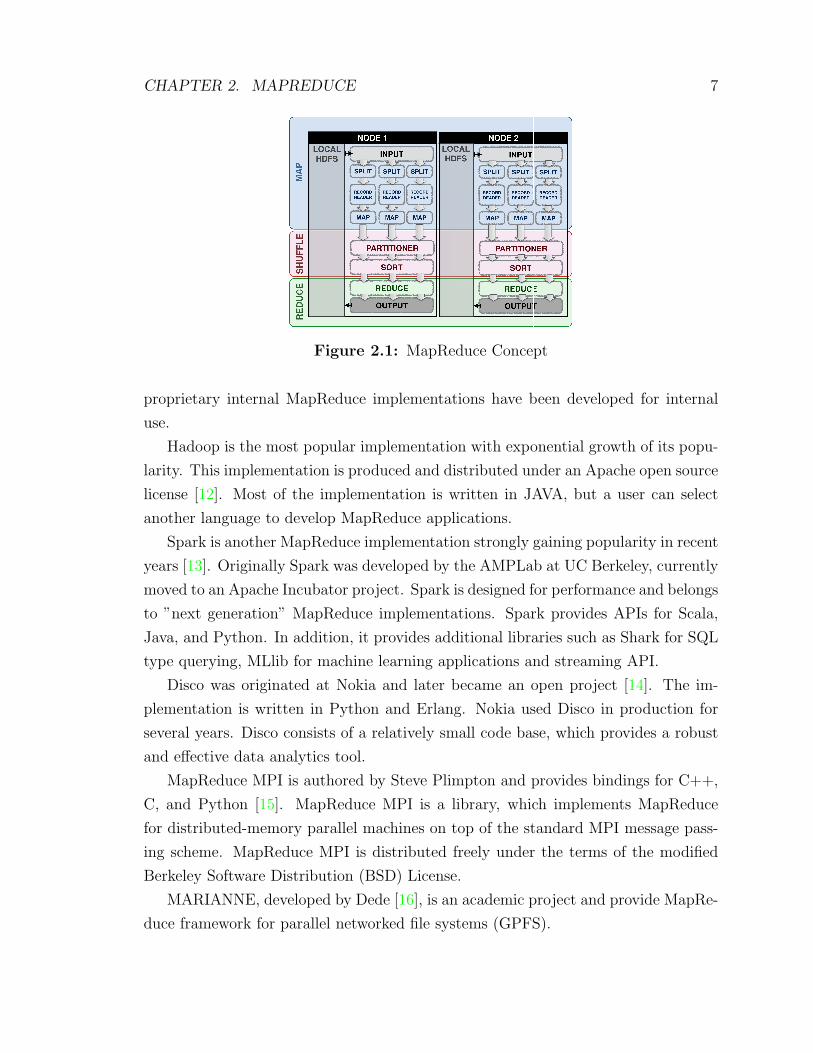
2.1 General Concept
In 2004, Dean and Ghemawat introduced the MapReduce programming concept as
an answer to the ever growing demand for fast and fault-tolerant Big Data process-
ing [5]. The authors aimed to create a simple yet effective programming model which
allows the programmer to focus on the computation task at hand abstracted from
the complications of a distributed system by such qualities as fault tolerance, load
balancing, data distribution and task parallelization. Concisely, MapReduce appli-
cations consist of map and reduce functions. First, all data is distributed among
processing units, nodes. Then, each assigned node executes a map function, which
creates key-value pairs from the data it has locally on the node. Next, the shuffle
stage, moves key-value pairs in such a way that all data units with the same keys
are located on the same node. Lastly, the reduce stage starts, and one or more re-
ducers compute the final output. The overall scheme of a process is shown in Figure
2.1. Note that distribution of the files among the nodes, and shuffling between map
and reduce stages is not exposed to the application developer and is facilitated by a
MapReduce framework.
2.2 MapReduce Implementations
Currently, there are a number of various MapReduce implementations including
Hadoop, Spark, Disco, MapReduce MPI, Phoenix, MARIANNE, and MARISSA.
In addition to the open source and academic projects named above, a number of
6
CHAPTER 2. MAPREDUCE 7
Figure 2.1: MapReduce Concept
proprietary internal MapReduce implementations have been developed for internal
use.
Hadoop is the most popular implementation with exponential growth of its popu-
larity. This implementation is produced and distributed under an Apache open source
license [12]. Most of the implementation is written in JAVA, but a user can select
another language to develop MapReduce applications.
Spark is another MapReduce implementation strongly gaining popularity in recent
years [13]. Originally Spark was developed by the AMPLab at UC Berkeley, currently
moved to an Apache Incubator project. Spark is designed for performance and belongs
to ”next generation” MapReduce implementations. Spark provides APIs for Scala,
Java, and Python. In addition, it provides additional libraries such as Shark for SQL
type querying, MLlib for machine learning applications and streaming API.
Disco was originated at Nokia and later became an open project [14]. The im-
plementation is written in Python and Erlang. Nokia used Disco in production for
several years. Disco consists of a relatively small code base, which provides a robust
and effective data analytics tool.
MapReduce MPI is authored by Steve Plimpton and provides bindings for C++,
C, and Python [15]. MapReduce MPI is a library, which implements MapReduce
for distributed-memory parallel machines on top of the standard MPI message pass-
ing scheme. MapReduce MPI is distributed freely under the terms of the modified
Berkeley Software Distribution (BSD) License.
MARIANNE, developed by Dede [16], is an academic project and provide MapRe-
duce framework for parallel networked file systems (GPFS).

CHAPTER 2. MAPREDUCE 8
Phoenix was originated in Stanford University and written in C++. The original
publication was produced in 2009 by Yoo and colleagues [17]. The Phoenix MapRe-
duce framework operates at the thread level. Apache Phoenix converts SQL query
into a series of HBase scans and then manages their execution in order to produce
regular JDBC result sets.
2.3 Specifics of the Apache Hadoop
The Apache Hadoop software library is an open-source software framework for reli-
able, scalable, distributed computing. It is designed for processing large data across
multiple computer nodes. Originally, Hadoop was based exclusively on the Map
Reduce programming model, but recently it expanded to support additional pro-
gramming models. The projects composed of multiple modules, including Hadoop
Common, Hadoop Distributed File System, Hadoop YARN and Hadoop MapReduce.
Hadoop Common is a module composed of common utilities and libraries respon-
sible for the support the other Hadoop modules. Hadoop Common assumes hardware
failures and must be handled by the software.
Hadoop Distributed File System (HDFS) is a data scalable, fault-tolerant, cost-
efficient storage module that provides high-throughput access to application data.
HDFS is a Java-based file system designed to span large clusters. HDFS offers a
number of valuable features such as rack awareness, minimal data motion, utilities,
rollback, standby NameNode, and operability.
Hadoop YARN (Yet Another Recourse Negotiator) is the most recent addition to
Hadoop architecture. The YARN module controls job scheduling and cluster resource
management. YARN could be viewed as the architectural center of Hadoop. The
YARN based architecture allowed Hadoop to evolve from being MapReduce based to
a more general large data processing platform. Together, HDFS and YARN form the
data management layer of the Apache Hadoop framework.
Currently, the Hadoop MapReduce module is a YARN-based large data processing
system based on MapReduce programming paradigm. The module provides machin-
ery to process Java and non-Java user applications written in MapReduce style func-
tional programming constructs for processing lists of data. MapReduce and HDFS
components were originally derived from Google’s MapReduce [5] and Google File
CHAPTER 2. MAPREDUCE 9
System (GFS) [6] papers, respectively. Original Apache Hadoop Map Reduce imple-
mentation had a number of limitations. For instance, the number of map and reduce
slots was predetermined for each of the task category at the beginning of the execution
and stayed static throughout the job. Therefore, if one of the tasks takes an exces-
sive amount of time, then the entire MapReduce job could be delayed. MapReduce
2.0 (MRv2), based on YARN architecture, has more effective resource management
system which partially overcomes limitations of the first version.
In addition to these key components, a number of Hadoop-related projects spawn
at Apache Hadoop, including Ambari, Avro, Cassandra, Chukwa, HBase, Hive, Ma-
hout, Pig, Spark, Tez, ZooKeeper. Each of the projects extend Hadoop functionality
or modify it in order to achieve optimal performance for a specific set of tasks.
For example, Cassandra is a highly scalable high-performance database with
proven fault-tolerance [18]. Cassandra’s Hadoop implements the same API as HDFS,
in order to achieve input data locality. Therefore, Cassandra is deployed seamlessly
with Hadoop. Cassandra is deployed by over 2500 companies, including Apple, Net-
flix, and Easou. The largest installations are composed of more than 75,000 nodes
and store over 10 PB of data.
Spark is a fast, general engine for large data distributed processing [13,19]. Spark
is compatible with Hadoop; hence, it could be deployed with Hadoop on top of the
Hadoop YARN, or as a standalone framework. Spark exhibits high performance
by operating on data reliably stored in memory, hence avoiding costly disk accesses.
Spark operation can be based on various data stores such as HDFS, Cassandra, HBase,
and S3.

Chapter 3
State of the Art
The performance of Hadoop jobs is sensitive to underlying hardware, network in-
frastructure, JVM configuration and the Hadoop parameter settings. All of these
challenges had been addressed by multiple research groups, revealing the importance
of each of the levels [9, 10, 20, 21]. While the first three levels could be addressed
once when a cluster is composed, the last must be attended each time when a new
MapReduce job is executed. Apache Hadoop exposes over 200 tunable parameters,
10% of which have a great impact on performance and effectiveness of the execu-
tion [8, 10, 22]. Exist so called Rule of Thumb (RoT) that are based on parameter
tuning guides released by manufacturers [23–25]. The difference in processing speed
between commonly used RoT settings and optimal configuration could be up to 100
fold [10,26].
In general, autotuning approaches can be divided in two categories: deterministic
and non-deterministic (heuristic). The first category relies on the meticulous explo-
ration of the search space, covering every possible solution. The method gives you
a guarantee than the found solution is the optimal one. Such a guarantee comes at
the cost of the long and extensive computation time and, in some cases, simply is
not feasible. The second category explores parts of the search space in such a way
that resulting values are most likely to be an optimal solution, but are not a guar-
antee. The advantage of this method reduced the amount of computation required.
Examples of deterministic solutions include A-tune, Manimal, Panacea, HAT and
Starfish [8, 9, 20,21,27,28].
The second category contains solutions based on heuristic approaches such as
Gunther, and machine-learning framework authored by Yigitbashi and colleagues
[10,22,29]. Hadoop autotuning was explored by multiple research groups.
10
CHAPTER 3. STATE OF THE ART 11
A language approach was explored, in 2009, by Schaefer and colleagues [20], who
developed an autotuning language for Map Reduce Atune-IL, which allows a user
to explore a selected set of tunable variables, such as the of threads or numbers of
map and reduce jobs, within defined by user limits. Atune-IL also allowed a user to
explore possible alternatives of the algorithmically blocks of the code. This approach
automates manual tuning to some extent, reduces search space and translates the
solution search to a simpler language tool; however, it requires a user to have the
expertise of Hadoop tuning in order to select important for the MR job tunables, to
set up limits and the size of the step for each tunable. Moreover, Atune-IL requires
a developer learn new syntax, specific to the language.
In 2010, one of the Hadoop creators, Michael Cafarella, together with Christo-
pher Re, introduced the wholly-automatic optimization framework, Manimal [21],
which uses static code analysis to detect MapReduce program semantics. The au-
thors combine widely practiced RDB tuning techniques with MR model resulting in
63% performance gain on selection tuning. The research suggests that selection tun-
ing success could be expanded on many other code structures such as projections,
and data compression.
Another way of approaching an autotuning problem is incorporating tuning algo-
rithms on the compiler level. An autotuning compiler for MapReduce, Panacea, was
proposed in 2012 by Liu and colleagues [27]. Panacea is able to optimize parameters
and MR-blocking with little or no input from the developer. Panacea claimed up to
three-fold performance improvement without user input. A fixed subset of tunable
parameters was explored within limits, set by a user or auto-determined by Panacea.
Parameters varied independently in a process of autotuning, which authors admit is
a suboptimal solution due to specifics of the search space landscape.
A history-based auto-tuning framework for MapReduce, HAT, was introduced by
Chen and colleagues in 2013 [28]. HAT tunes the weight of each stage of a map and
a reduce task according to value of the tasks in the history and orchestrates Hadoop
back up task execution according to the current and historical weights of the tasks,
resulting in 37% improvement of execution time.
Starfish is a cost-based Hadoop autotuning framework developed at Duke Uni-
versity by Babu and colleagues [8, 9]. Starfish takes into account different levels of
MapReduce program, adjusting various decision points, which include provisioning,
CHAPTER 3. STATE OF THE ART 12
optimization, scheduling, and data layout. The heart of the framework is a What-
if engine, which employs a combination of simulation and model-based estimation.
The authors succeeded in applying a popular in relational database tuning cost-base
towards the MapReduce concept.
In 2013, Liao and colleagues analyzed model-based approaches for Hadoop MapRe-
duce optimization and identified major limitations [10]. The research group proposed
and implemented, Gunther, a search-based auto-tuner. The comparison of several
global search algorithms leads to the selection of GA as a search strategy. The mod-
ified GA was evaluated on two clusters. Experimental results demonstrated that
Gunther achieves near-optimal performance in a small number of trials (<30) and
yields better performance improvement than rule-of-thumb settings and a cost-based
auto-tuner.
As another example of the heuristic approach published in the same year as Gun-
ther, is research conducted by Bezhad and colleagues. They also demonstrated that a
GA -based parameter search combined with dynamically intercepted HDF5 calls can
result in up to 100 fold I/O write speedup for some tasks [26].
Another niche of heuristic algorithms, machine learning, was explored by Yigit-
bashi and colleagues [22], who analyzed various machine learning-based performance
models. The analysis was conducted on two standard Hadoop benchmarks: sort and
word count, with datasets of various sizes and led to a conclusion that Support Vector
Regression exhibits the best performance between machine learning methods. The
Support Vector Regression based autotuner also outperforms a well-known, cost-based
auto-tuner, Starfish.
Another search-based evolutionary computation approach was conducted by Filho
and colleagues, in 2014 [29]. They propose an adaptive tuning mechanism that enables
the setting of specific resources to each job within a query plan. A data structure
mapping a job to tuning solutions is created based on an analysis of the source code
and log files.
Notice that all presented solutions are developed based on the off-line autotuning
concept. Therefore, these solutions require multiple executions of the full job in order
to produce optimized tuning values. During the work on the current project a research
introducing mrOnline was published by Li and colleagues [30]. mrOnline is an on-
line autotuner for the YARN framework, which was evaluated on a 19-node cluster
and claims up to 30% performance improvement compared to the default settings.
CHAPTER 3. STATE OF THE ART 13
mrOnline built on top of HDFS and the cost evaluation is done via autotuner daemons
running in each of the name nodes. Moreover, the autotuning engine is powered upon
a pre-programmed set of rules. Unfortunately, mrOnline was built in collaboration
with IBM research; hence, details of implementation and the source code were not
made available to the public.
The presented selection of autotuning investigations show that Hadoop auto-
tuning is, indeed, a very active research field. There is multiple approaches tested
under different circumstances. A comparison between such solutions, or even direc-
tions of autotuning approach, is extremely difficult due to specifics of domain and
overall in the maturity of Hadoop, and MapReduce, in general. It is clear that a pure
modeling and cost-based approach does not reach a desirable level of improvement
and, in some cases, its flaws are especially visible [8, 10]. Yet, heuristic approaches,
despite the achievement of superior results, require multiple iterations, which, con-
sidering the size of computation for an average MR job, make real life employment
of such concepts unfeasible [22]. Nevertheless, all the publications, excluding mrOn-
line, persuade the off-line autotuning approach, which limits application for the final
product. The emergence of on-line tuning research, mrOnline, confirms that real time
tuning is a highly desirable, yet underexplored direction, of Hadoop/YARN automatic
tuning.

Chapter 4
Autotuning Algorithms
A number of the approaches were applied to autotuning in general and, in particular,
to the Hadoop autotuning. In this chapter, the most popular and effective algorithms
will be presented.
4.1 Simulated Annealing
Simulated annealing is an extremely popular local search algorithm. The popularity
of simulated annealing roots in the simplicity of the concept, the low computational
requirements and relatively good performance. The concept was derived from the
physical process of the annealing solids. In metallurgy, annealing raises its temper-
ature above re-crystallization mark, followed by cooling below it. It is extremely
important that the cooling process is conveyed in a slow, careful manner. The de-
sired state of the solid is obtained only if heating was sufficiently high and cooling
was sufficiently slow, allowing particles to arrange in a highly structured grid, which
corresponds to the lowest energy level. The cycle could be repeated numerous times.
First, the concept of annealing was translated to computer science in 1983 by
Kirkpatrick [31] and independently by Cerny in 1985 [32]. Translation from physical
to computer science optimization problem is achieved by the assumption of the two
following equivalences. First, solution vectors in an optimization problem are equiva-
lent to states of the physical system. Second, the cost of the solution, determined by
the cost function, is equivalent to the energy of a physical state. Moreover, the tem-
perature role is played by the control parameter. Originally, the simulated annealing
algorithm was very close to the physical model; later in its development, it deviated
from it to the higher abstraction level.
14

CHAPTER 4. AUTOTUNING ALGORITHMS 15
Let us view the parameter optimization as a minimization problem. Note this
easily translated into a maximization problem; hence, it could be used without loss
of generality. The algorithm probabilistically re-samples the problem space. The
acceptance of new samples is based on the cost and probabilistic components. Over
the execution time of the algorithm, ”temperature” or control criteria (ck) decreases
from relatively large values to almost zero. If the cost of a new parameter is greater or
equal to the current cost, it is accepted and becomes a new current (see Algorithm 1:
lines 6-7). Otherwise, the probability of acceptance of a new value depends on value
of exp((f(i)f(j))/c) through comparison of that value to a random number between 0
and 1 (see Algorithm 1: line 8). After each iteration, the new length and new control
value are calculated (see Algorithm 1: lines 12-13). Other steps of the algorithm
are routine. It starts from the initialization of the starting state, which consists of
a current parameter (istart), initial control parameter (c0) and initial length (L0).
Length value determines how many samples will be taken at the particular iteration.
Iterations are repeated until a stopping condition is met (see Algorithm 1: line 3).
Each iteration has a number of samples generated (see Algorithm 1: line 5) and
checked against current value. The number of samples is determined by the length
value (see Algorithm 1: line 4).
Algorithm 1 Simulated Annealing
Require: istart, c0, L0
k ← 0i← istartwhile !STOP − CONDITION − TRUE do
for L← 1 TO Lk doGENERATE(j FROM Si)if COST (j) ≤ COST (i) theni← j
else if exp(COST (i)−COST (j)ck
) < random[0, 1) theni← j
end ifk + +CALCULATE-LENGTH (Lk)CALCULATE-CONTROL(ck)
end forend while
CHAPTER 4. AUTOTUNING ALGORITHMS 16
Since its introduction, simulated annealing had been successfully applied to nu-
merous problems in a wide variety of research areas including molecular physics, code
processing, VLSI design, operations search and autotuning. An example of an auto-
tuning application of simulated annealing is the Panda project [11] studied automatic
performance optimization for collective I/O.
The good performance, simplicity of implementation, applicability to a wide range
of the problems and flexibility resulted in the popularization of simulated annealing
algorithm. Nevertheless, the application of simulated annealing to concrete prob-
lems requires tuning of itself. In particular, finding an optimal cooling schedule and
localizing domain neighborhoods for it could lead to extensive experimental overload.
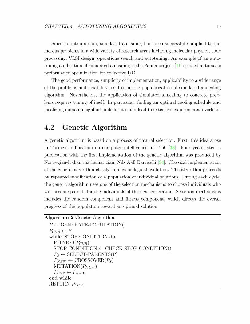
4.2 Genetic Algorithm
A genetic algorithm is based on a process of natural selection. First, this idea arose
in Turing’s publication on computer intelligence, in 1950 [33]. Four years later, a
publication with the first implementation of the genetic algorithm was produced by
Norwegian-Italian mathematician, Nils Aall Barricelli [34]. Classical implementation
of the genetic algorithm closely mimics biological evolution. The algorithm proceeds
by repeated modification of a population of individual solutions. During each cycle,
the genetic algorithm uses one of the selection mechanisms to choose individuals who
will become parents for the individuals of the next generation. Selection mechanisms
includes the random component and fitness component, which directs the overall
progress of the population toward an optimal solution.
Algorithm 2 Genetic Algorithm
P ← GENERATE-POPULATION()PCUR ← Pwhile !STOP-CONDITION do
FITNESS(PCUR)STOP-CONDITION ← CHECK-STOP-CONDITION()PS ← SELECT-PARENTS(P)PNEW ← CROSSOVER(PS)MUTATION(PNEW )PCUR ← PNEW
end whileRETURN PCUR
CHAPTER 4. AUTOTUNING ALGORITHMS 17
The typical genetic algorithm consists of the five main steps: generation of the
original population; evaluation of the each of the individual with a fitness function;
selection of the parents according to a selection function; production of the next gener-
ation with optional employment of crossover and mutation functions; check stopping
conditions and, if they are satisfied, return the best solution, so far. Commonly used
stopping conditions are composed of optimal, or near to optimal, solutions and gener-
ation number maximum. The last four steps are repeated until the stopping condition
is met.
Strong points of the genetic algorithm approach include the ability to reach a near
optimal solution and the algorithms flexibility and suitability for complex problems
with multiple objectives. Moreover, the effective selection of the population size,
selection, crossover and mutation methods provides an effective mechanism, which
avoids local minimal in non-unimodal complex search surface. The downsides of a
genetic algorithm methodology include multiple repetitions, which could be unsuit-
able for real world problems. For example, if a population consists of 12 solutions,
which is an extremely small population, and 30 generations are required to reach a
near optimal solution, then 360 evaluations are required, in total. As these evalua-
tions run sequentially, for a 5-minute job, it will take 30 hours of tuning to discover
the best solution and, for 1-hour job, it will take 15 days of continuous computation.
The decrease in population size or number of generations has a negative effect on the
results. Another problem with the genetic algorithm approach is that the approach is
extremely sensitive to the selection of its own parameters, such as choice of the fitness,
selection, mutation and crossover methods, along with the previously mentioned size
of population and maximal number of generations parameters. Hence, tuning of the
autotuning algorithm becomes an additional task.
The practical application of genetic algorithms spreads widely across many fields
including various optimizations and automatic tuning problems in engineering, com-
putational science, bioinformatics, signal and image processing, risk analysis, robotics,
economics, molecular chemistry, computational physics and many others. During re-
search of the existent work of MapReduce and Hadoop automatic tuning, a number
of solutions employed genetic algorithm. For instance, the Gunther project developed
by Liao and colleagues explores parameter space by means of a genetic algorithm and
achieves near-optimal performance [10]. Another example of an auto-tuning system,
which employs genetic algorithm for autotuning is a parameter optimization system

CHAPTER 4. AUTOTUNING ALGORITHMS 18
for I/O performance of HDF5 application developed by Bezhad and colleagues [35].
This system achieves impressive speedups up to fifty times faster than the baseline.
4.3 Hill Climbing
Hill climbing, also known as greedy local search, is a popular gradient-based heuristic
algorithm often used for optimization problems. The name of the algorithm comes
from its analogy with the climbing of a hill. First the algorithm is starting at the base
with a sub optimal solution, which needs improvement. Than continue to improve it
with small steps in direction of the top of the hill, the optimal solution.
Algorithm 3 Hill Climbing
VCUR ←GENERATE-START()while !STOP-CONDITION-TRUE doECUR ← EVAL(VCUR)VN ←GENERATE-NEIGHBOR(VCUR)EN ← EVAL(VN)if EN > ECUR thenVCUR ← VN
STOP-CONDITION-TRUE ← TRUEend if
end while
The hill climbing algorithm starts at a given point in the search space, evaluates
it, then produces one or more neighbours of that point, then also evaluates these
solutions with specific fitness function. Next, current point fitness is compared to the
fitnesses of the neighbours and the best is selected to be the next current point. The
cycle is repeated until stopping conditions are met. Stopping conditions could take
effect when the maximum number of iterations is reached or the best point of the
neighbourhood is found. In other words, no local move would improve the solution.
That approach makes hill climbing to be extremely sensitive to producing suboptimal
solutions by ”getting stuck” at a local optimal solution. One of the solutions for this
problem is to allow the algorithm to proceed to equal or worse than current solutions,
keeping track of the current best solution. In this case, the stopping condition could
have a different set of rules. This relaxed approach is a key component of local
search methods for the Boolean specifiability (SAT) problems, such as GSAT and
CHAPTER 4. AUTOTUNING ALGORITHMS 19
Walksat [36]. Another way to escape local optimal solutions is to restart the climb
from a previously visited point with an unexplored neighbor or have multiple climbers
exploring the search space simultaneously. These are stochastic variations of a hill
climbing algorithm.
A great example of an effective variation of the hill climbing algorithm is an award-
winning Late Acceptance Hill Climbing algorithm [37]. The main idea of the Late
Acceptance Hill Climbing algorithm is that it accepts a candidate solution if it is not
worse than the solution, which was ”current” several steps before. It is impressive
that such a simple concept outperformed many complex machine learning approaches.
Therefore, modified hill climbing algorithms produce surprisingly good results, de-
spite their simplicity and surpass the performance of many other much more complex
heuristics. Moreover, most of the optimizations do not require as large a number of
executions as some other methods, such as genetic algorithms do. Another advantage
of the hill climbing technique is that it does not depend on the quality of a cooling-
schedule, selection, crossover, and mutation methods, size of population and other
parameters that greatly affect previously discussed algorithms.
Chapter 5
Hadoop Source Code
5.1 Overall Architecture
Most Hadoop source code is written in Java. Critical code is written in C, for perfor-
mance reasons. Hadoop 2.6.0 can be run on various Linux distributions and Windows.
The original Hadoop framework was composed of two layers: MapReduce and HDFS.
The MapReduce layer is the computational layer. HDFS is the layer responsible for file
storage and organization. Both layers are based on master/slave node architecture.
Such architecture simplifies design by providing the global knowledge base, which
includes job scheduling and block placement information. The disadvantage of this
architecture is that the master node becomes a single point of failure. In some cluster
configurations, the situation could be improved by a hot standby for the master node.
Nevertheless, Hadoop clusters are extremely robust against slave node failures. Slave
node data is duplicated and could be reconstructed by remaining slave nodes in the
event of failure. While in the traditional distributed computing model, data is moved
to the place of computation; in MapReduce the computation is moved to the data.
Therefore, high data throughput with minimal data movement, so desirable for Big
Data processing, is achieved. Since Apache Hadoop 2.2.0, there are two implementa-
tions of the MapReduce programming model available: the original Apache Hadoop
MapReduce model, and the new Apache Hadoop Yet-Another-Resource-Negotiator
(YARN) model (Figures 5.1, 5.2).
20
CHAPTER 5. HADOOP SOURCE CODE 21
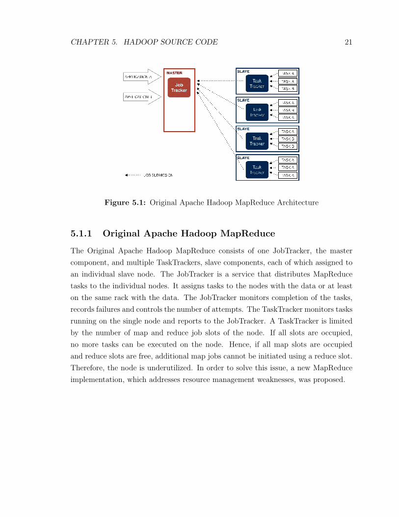
Figure 5.1: Original Apache Hadoop MapReduce Architecture
5.1.1 Original Apache Hadoop MapReduce
The Original Apache Hadoop MapReduce consists of one JobTracker, the master
component, and multiple TaskTrackers, slave components, each of which assigned to
an individual slave node. The JobTracker is a service that distributes MapReduce
tasks to the individual nodes. It assigns tasks to the nodes with the data or at least
on the same rack with the data. The JobTracker monitors completion of the tasks,
records failures and controls the number of attempts. The TaskTracker monitors tasks
running on the single node and reports to the JobTracker. A TaskTracker is limited
by the number of map and reduce job slots of the node. If all slots are occupied,
no more tasks can be executed on the node. Hence, if all map slots are occupied
and reduce slots are free, additional map jobs cannot be initiated using a reduce slot.
Therefore, the node is underutilized. In order to solve this issue, a new MapReduce
implementation, which addresses resource management weaknesses, was proposed.

CHAPTER 5. HADOOP SOURCE CODE 22
Figure 5.2: Apache Hadoop Yet-Another-Resource-Negotiator (YARN) Architec-ture
5.1.2 Apache Hadoop Yet-Another-Resource-Negotiator
(YARN)
YARN is based on idea of splitting JobTracker’s responsibilities for resource man-
agement and job scheduling/monitoring between two daemons. YARN replaces Job-
Tracker by the global ResourceManager, which communicates with per-application
ApplicationManagers to allocate resources for the particular application. Moreover,
ApplicationManager monitors the execution of the tasks via communication with
individual NodeManagers, each of which is assigned to a particular node.
The allocation of the resources in YARN is based on the notion of container. The
Container represents an allocated resource in the cluster. The Container incorporates
resource elements such as memory, CPU, disk, and network. The ResourceManager is
the sole authority to allocate any Container to applications. The allocated Container
is always on a single node and has a unique Container ID. Each container has a
globally unique Container ID, and stores the unique ID of the specific node it was
allocated on, the NodeID. More over aContainer has Resource and Priority objects,
which contains detailed information about the container’s structure.
Containers are assigned to the application via a Resource Scheduler. YARN has
a modular scheduler, which deals exclusively with the allocation on the resources in
given priority to the applications. Different schedulers are provided by the Hadoop
CHAPTER 5. HADOOP SOURCE CODE 23
framework. The default YARN scheduler is the Capacity Scheduler, which is designed
to run Hadoop applications as a shared, multi-tenant cluster in an operator-friendly
manner while maximizing the throughput and the utilization of the cluster. Scheduler
class can be changed via a yarn− site.xml configuration file. For example, the Fair
Scheduler allows YARN applications to share resources in large clusters fairly.
A Resource calculator used by a scheduler could be chosen through the setting of
Resource Calculator property in the scheduler configuration file. The default sched-
uler is based only on memory parameter, while the Dominant Resource Calculator
uses chosen Dominant-resource to compare multi-dimensional resources such as mem-
ory and CPU. Note, that a scheduler in YARN does not perform monitoring or track
the status for the application. Hence, a scheduler offers no guarantees on restarting
of failed tasks. Moreover, a YARN system reuses an existent MapReduce network,
which ensures compatibility.
5.2 Hadoop on YARN
The current YARN-based Hadoop is a complex multilayered ecosystem. It could be
viewed in layers as shown in Figure 5.3. The first layer is the file system, respon-
sible for storage detection of failures and quick automatic recovery. The file system
is represented mostly by HDFS, which could be specialized with additional pack-
ages implemented on top of it, such as HBase. The next layer consists of YARN,
which operates on top of the storage layer and is responsible for main logic and com-
putations. YARN solely composes the cluster compute layer. YARN applications
are built immediately on top of YARN and interact with it by mean of YARN API
creating YARN applications layer. This architecture widen horizons of Hadoop com-
putation models from MapReduce only to a virtually limitless number of Big Data
programming concepts, which could be implemented within the Hadoop ecosystem.
In addition to MapReduce, the most popular of the currently implemented YARN
applications are Spark and Tez. On top of these applications, users can build their
own applications, or go one level higher and use the second application layer, which
consists of applications, which do not interact with YARN directly, such as Pig, Hive,
Cascading, Crunch.

CHAPTER 5. HADOOP SOURCE CODE 24
Figure 5.3: Apache Hadoop on YARN Structure
5.2.1 YARN Application Execution Overview
The application execution starts with a client contacting the Resource Manager, re-
questing an Application Master. An Application Master instance must run on one
of the cluster nodes. In order to allocate resources for an Application Master, the
Resource Manager contacts node managers and determines a node with available suf-
ficient resources or, in other words, has a suitable container. Next, if an application is
small and container resources are sufficient to complete the job, the application runs
locally on the node. Otherwise, more resources are allocated. In order to acquire ad-
ditional resources, an Application Master calculates the number and configuration of
additional containers needed for the application, then requests them from the resource
manager. These containers could be allocated on different nodes and an application
will run on a distributed system. In the current paper, research concentrated on the
2.2 version Hadoop MapReduce. Therefore, let us consider a Hadoop MapReduce on
YARN job in detail.
5.2.2 MapReduce Job Execution Overview
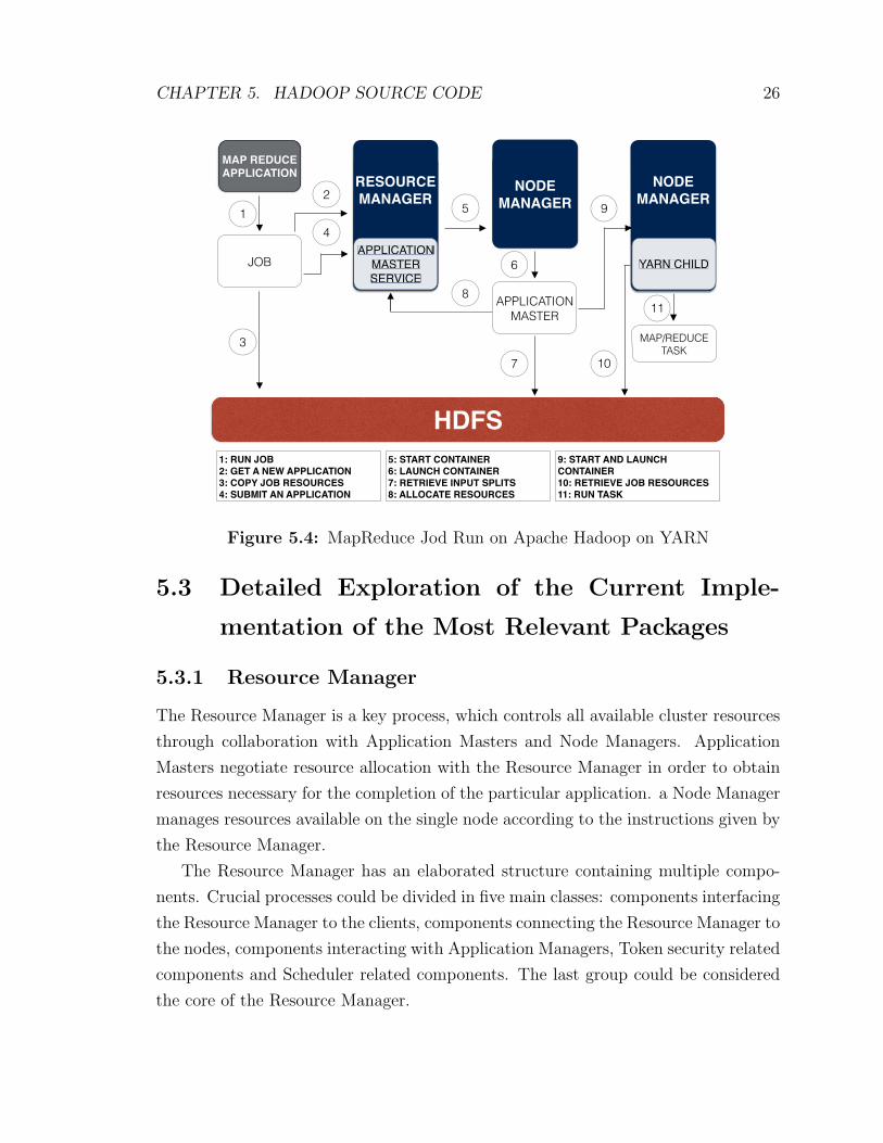
MapReduce job execution could be divided in four consecutive steps: job submission,
job initialization, task assignment and task execution.
The first step is job submission; it starts from a call of a submit method of a
CHAPTER 5. HADOOP SOURCE CODE 25
Job instance. Within the submit method, a JobSubmitter instance is created and its
submitJobInternal method is executed. After job submission, waitForCompletion
method receives updates on job progress every second and outputs changes to the
console. The JobSubmitter requests a new application ID (job ID) from the re-
source manager, checks the job’s output specifications, computes the job’s input
splits, copies required for the job resources and, at last, submits the job by means of
submitApplication method of resource manager.
The second step is job initialization, in which the resource manager delegates
the request to a YARN scheduler, which allocated a container for the application
master process, and the resource manager launches it under a node manager of the
particular node. The application master (MRAppMaster class)retrieves previously
computed input data splits and created map tasks, accordingly. Usually, a one map
task per one split. Next, reduce tasks are created based on mapreduce.job.reduces
property. All tasks are assigned a globally unique task ID.
The application master determines if this job uberized and can be completed
within the same JVM, sequentially. If not, additional containers will be requested in
the next step.
The third step is task assignment. First, requests for all map tasks are di-
rected to the resource manager. Requests for reduce tasks issued after at least
5% of map tasks were completed. By default, each task is allocated 1024MB
of memory and one virtual core. These parameters could be modified by means
of configuration settings: mapreduce.map.memory.mb, mapreduce.map.cpu.vcores,
mapreduce.reduce.memory.mb, and mapreduce.reduce.cpu.vcores. These settings
could be configured for each individual job and limited by minimum and maximum
settings set for the YARN cluster configuration. By means of a YARN scheduler, the
resource manager assigns specified containers to the tasks and returns the list of these
containers to the Application Master.
The forth step is task execution. The Application Master contacts the node man-
agers of the nodes, which have the assigned containers and start the containers. Tasks
are instances of the YarnChild class. The next task localizes all necessary resources
and then has the map or reduce task executed.
CHAPTER 5. HADOOP SOURCE CODE 26
MAP REDUCE APPLICATION
JOB
RESOURCE MANAGER NODE
MANAGER
APPLICATION MASTER
MAP/REDUCE TASK
12
3
4
5
6
7
8
9
10
HDFS
NODE MANAGERNODE
MANAGERNODE
MANAGERRESOURCE MANAGER
APPLICATION MASTER SERVICE
1: RUN JOB2: GET A NEW APPLICATION3: COPY JOB RESOURCES4: SUBMIT AN APPLICATION
5: START CONTAINER 6: LAUNCH CONTAINER7: RETRIEVE INPUT SPLITS8: ALLOCATE RESOURCES
YARN CHILD
11
9: START AND LAUNCH CONTAINER10: RETRIEVE JOB RESOURCES 11: RUN TASK
Figure 5.4: MapReduce Jod Run on Apache Hadoop on YARN
5.3 Detailed Exploration of the Current Imple-
mentation of the Most Relevant Packages
5.3.1 Resource Manager
The Resource Manager is a key process, which controls all available cluster resources
through collaboration with Application Masters and Node Managers. Application
Masters negotiate resource allocation with the Resource Manager in order to obtain
resources necessary for the completion of the particular application. a Node Manager
manages resources available on the single node according to the instructions given by
the Resource Manager.
The Resource Manager has an elaborated structure containing multiple compo-
nents. Crucial processes could be divided in five main classes: components interfacing
the Resource Manager to the clients, components connecting the Resource Manager to
the nodes, components interacting with Application Managers, Token security related
components and Scheduler related components. The last group could be considered
the core of the Resource Manager.
CHAPTER 5. HADOOP SOURCE CODE 27
5.3.2 Scheduler Related Components
Scheduler-related components are the heart of the Resource Manager and carry out
the main functionality which is supported by the rest on the modules. The most sig-
nificant classes of this group are ApplicationsManager, ApplicationACLsManager,
ApplicationMasterLauncher, Y arnScheduler and ContainerAllocationExpirer.
ApplicationsManager orchestrates all the submitted applications, including com-
pleted applications, and responds to all users requests made via command line inter-
face. ApplicationACLsManager responds to the restricted administrator and au-
thorized client requests, and maintains and enforces the Access Control Lists (ACL)
per each application. ApplicationMasterLauncher is responsible for maintaining a
thread pool to launch new Application Masters, and is responsible for cleaning up
on Application Master termination. The YarnScheduler is responsible for allocating
resources for all current applications taking into account to cluster resource limita-
tions. ContainerAllocationExpirer controls the appropriate launch of all allocated
containers on the corresponding nodes in order to optimize cluster utilization.
5.3.3 Client Interfacing Components
This group composed of two services dedicated to two types of users: Client Service
and Admin Service. Client Service is a client interface available to all users, which
handles all RPC requests, such as application submission, application termination,
obtaining queue information, and cluster statistics. Admin Service is a special in-
terface dedicated to give high priority to requests issued by the operator. Hence,
important operations, such as the refreshing node list or the queues configuration,
are not waiting in the same queue as routine users requests.
5.3.4 Connecting to the Nodes Components
The Resource Tracker Service is the component that responds to Remote Procedure
Calls (RPC) from the nodes. It facilitates the registration of new nodes, rejection
of the requests from any invalid or decommissioned nodes, collection of the node
heartbeats and redirection of this information to the Scheduler. The Resource Tracer
Service intensively interacts with other two components of the Resource Manager,
which also belong to this category: Node Manager Liveliness Monitor and Nodes List
Manager.
CHAPTER 5. HADOOP SOURCE CODE 28
A Node Manager Liveliness Monitor tracks live nodes and notifies the Resource
Manager of the dead nodes. The Node Manager Liveliness Monitor achieves that by
monitoring individual nodes heartbeat time. If the time that passes since the nodes
last heartbeat is greater than the configured interval of time, the node is marked
dead and is expired by the Resource Manager. Moreover, all the containers currently
running on an expired node are marked as dead and no new containers are scheduled
on it.
The Nodes List Manager is a collection of valid and excluded nodes. Based on
the host configuration files specified via yarn.resourcemanager.nodes.include-path and
yarn.resourcemanager.nodes.exclude-path, the initial list of nodes is created. During
Hadoop run, the Nodes List Manager is also responsible to move decommissioned
nodes from the included nodes list to the excluded nodes list.
5.3.5 Application Masters’ interacting components
The Application Master Service is the key component that handles responses to RPCs
from all the Application Masters. The Application Master Service is responsible for
wide variety of tasks, such as the registration of a new Application Master, con-
trolling container allocation and deallocation requests from all running Application
Masters, forwarding them to the Scheduler and processing termination and unregister
requests from a finishing Application Master. The application Master Service works
closely with an Application Master Liveliness Monitor, another Application Master
communicating component.
An Application Master Liveliness Monitor is a component that assists the man-
agement of the list of Application Masters and their statuses. An Application Master
Liveliness Monitor monitors each Application Master and its last heartbeat time.
Similarly to the node management scheme, if an Application Master does not pro-
duce a heartbeat within a configured interval of time it is marked as dead and is
expired by the Resource Manager. Next, all the containers currently running or allo-
cated to that particular Application Master are also marked as dead. After that, the
Resource Manager schedules the same Application Master to run on a new container.
The number of such restarts is limited by configurable value.
CHAPTER 5. HADOOP SOURCE CODE 29
5.4 Application Master
An Application Master is a component responsible for the orchestration of the sin-
gle job. An Application Master is initiated when a job started. Hence, multiple
instances of the Application Master class could coexist. A user is provided with Ap-
plicationMaster and MRAppMaster classes. The second class is designed to serve
Map Reduce type of jobs. Moreover, a user is given functionality to create custom
Application Master extending Application Master interface. Nevertheless, the main
Application Master functionality must be supported in all variations.
When an application initiated the Resource Manager invokes the Application Mas-
ter Launcher method, which requests container for an Application Master process.
When it obtains the container, it starts an Application Master process in it and
records bookkeeping information about the newly created Application Master in the
Resource Master. Next the Application Master registers itself with the Resource
Manager. The registration process includes assigning host ports, job status and job
history tracking URLs, etc.
During application execution, an Application Master produces regular heartbeats
to inform the Resource Manager of its condition. The heartbeats are an impor-
tant part of fault resistance and the recovery mechanism. Moreover, the heartbeat
mechanism is facilitated by an allocation request protocol (ApplicationMasterProto-
col.allocate in org.apache.hadoop.yarn.api.protocolrecords.AllocateRequest). An Ap-
plication Master requests, from the Resource Master, a number of containers with
specified memory capacity operating on a particular number of virtual cores. These
values are consistent throughout the execution and are calculated by Hadoop based
on configuration files. Moreover, the Application Master could specify a locality re-
quest and a level of priority should be given to the location request. The Resource
Manager responds with a set of newly allocated containers, completed containers and
a current state of available resources. Note that each request includes all the con-
tainers necessary for the completion of the job; hence, the returned set of values just
partially fulfills the request, in most of the cases. A Resource Requests communicated
through the Application Master Service class of the Resource Manager.
Allocated containers are processed by an Application Master by means of the Con-
tainer Launch Context method, which specifies container ID, local resources required
by the executable, the environment to be setup for the executable, commands to ex-
ecute and other specifics for each container. Next, a launched container is submitted

CHAPTER 5. HADOOP SOURCE CODE 30
to a Start Container Request method in the Container Management Protocol, which
executes previously set commands and starts the container.
The control of the containers is facilitated by querying of the Resource Manager
via an Application Master Protocol allocate method or via Container Management
Protocol by querying for the status of the allocated container’s ContainerID. On the
job completion, the Application Master sends a Finish Application Master Request
to the Resource Manager, which unregisters the Application Master and initiates the
application completion process.
MRAppMaster, in addition to the previously described functionality, has a his-
tory server and segregates requests for a map and a reduce container. The reduce
containers request is delayed, and the size of the delay is set by configuration. On
initialization, the MRAppMaster retrieves all the input splits from file system. Then,
the Application Master computes all the map tasks for each input split, while the
number of reduce tasks is determined by the configuration. Upon job completion, the
job history server archives all job information.
5.5 YARN Schedulers
A YARN Scheduler allocates resources to applications according to a specific policy.
Hadoop 2.2 is distributed with 3 built in YARN Schedulers: FIFO, Fair and Capacity
Scheduler. Moreover, a user provided with an extendable API for the cases when the
custom Scheduler is required. Specifics of each of the Hadoop YARN Schedulers are
described below.
5.5.1 The FIFO Scheduler
FIFO (First In First Out) is the simplest of the schedulers; it follows a well-known
scheme by placing applications in a queue, then running them in the order of submis-
sion. Therefore, first, all requests for the first application are allocated, and only after
that are requests for the next one considered. The strength of the FIFO approach is
its simplicity and absence of additional configuration settings. Nevertheless, its per-
formance is not ideal and it is not recommended for a shared cluster. For example, if
a small job is submitted to a FIFO scheduler after a large one, it will not be served
until the large job is run to completion.
CHAPTER 5. HADOOP SOURCE CODE 31
5.5.2 The Capacity Scheduler
The Capacity Scheduler requires a configuration file, which determines a hierarchy
among users or organizations. Each organization is allocated a certain part of the
overall cluster capacity and assigned a designated queue. Users within organizations
could be farther divided in groups with different priorities. Inside the single user
group tasks follow the FIFO schedule. Overall, the Capacity Scheduler supports
multiple requests, provides security, elasticity, resource-based scheduling, and con-
figurable job priorities. Hence, it provides an administrator with a number of fine
tuning mechanisms to optimize cluster deployment in a multi-tenant environment.
5.5.3 The Fair Scheduler
The Fair Scheduler is also recommended for resource sharing on a large multi-tenant
Hadoop cluster. The Fair scheduler assures that all jobs get an equal share of the total
cluster resources. In the event of the job number change, when a job is completed
or a new job is initiated, the fair scheduler redistributes the resources according to
the recalculated proportions. Hence, the cluster is used to full capacity at any given
moment. The downside of the method is the delay in obtaining new resources, while
resources are released and room made for the new job pool. The fair scheduler could
be fine-tuned with job priorities, which are used as weights to determine the fraction of
total resources that should be made available to a job. A number of parameters could
be provided to a Fair Scheduler by means of the configuration file, including enabling
preemption, pool name property, allocation file name, and per job load manager.
5.6 Tunable Hadoop Parameters
Hadoop exposes hundreds of parameters and a small number of them have an ex-
tremely high impact on the performance and could not be derived from a static for-
mula. Currently, the parameters must be obtained through manual iterative tuning.
Therefore, only one set of parameters could be tested simultaneously. Information
about tunable parameters is scattered among multiple sources such as white papers,
Hadoop, Hortonworks and Cloudera web sites, and blog posts of credible profession-
als. Parameters that have a great impact on the cluster resource utilization and total
execution time could be divided in four main categories: MapReduce related, YARN
CHAPTER 5. HADOOP SOURCE CODE 32
specific, HDFS related and core settings, which influence general configuration.
The first category includes mapreduce.job.reduces, mapred.child.java.opts,
mapreduce.map.output.compress, mapreduce.map.cpu.vcores, mapre-
duce.reduce.cpu.vcores, mapreduce.reduce.memory.mb, mapreduce.map.memory.mb.
The second category includes yarn.nodemanager.resource.memory-
mb, yarn.nodemanager.resource.cpu-vcores, yarn.nodemanager.resource.
npercentage-physical-cpu-limit, yarn.scheduler.maximum-allocation-mb,
yarn.scheduler.minimum-allocation-mb, yarn.scheduler.maximum-allocation-
vcores, yarn.scheduler.minimum-allocation-vcores. The third category includes
dfs.datanode.handler.count, dfs.replication, dfs.blocksize. Finally, the fourth
category includes io.file.buffer.size and file.blocksize.
The parameters that are responsible for the number and size of YARN contain-
ers for map tasks are mapreduce.map.memory.mb (mapred-site.xml) and mapre-
duce.map.cpu.vcores (mapred-site.xml), mapreduce.reduce.memory.mb (mapred-
site.xml), mapreduce.reduce.cpu.vcores (mapred-site.xml). This list of parameters
was selected based on previous Hadoop automatic tuning efforts and currently rec-
ommended for tuning parameters on the Apache Hadoop official web page [38] and
the Hortonworks web page [39]. Previous work on Hadoop and MapReduce automatic
tuning supports the given subset of the parameters as well as displays the necessity
of autotuning these particular parameters and their combinations [8,9,20,21,26–29].
The description of the parameters, the configuration file they are set in and the default
values are presented in detail in Table 5.1.
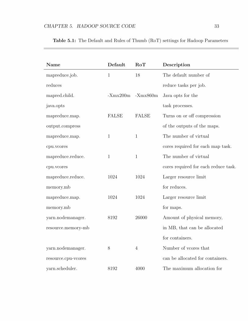
CHAPTER 5. HADOOP SOURCE CODE 33
Table 5.1: The Default and Rules of Thumb (RoT) settings for Hadoop Parameters
Name Default RoT Description
mapreduce.job. 1 18 The default number of
reduces reduce tasks per job.
mapred.child. -Xmx200m -Xmx860m Java opts for the
java.opts task processes.
mapreduce.map. FALSE FALSE Turns on or off compression
output.compress of the outputs of the maps.
mapreduce.map. 1 1 The number of virtual
cpu.vcores cores required for each map task.
mapreduce.reduce. 1 1 The number of virtual
cpu.vcores cores required for each reduce task.
mapreduce.reduce. 1024 1024 Larger resource limit
memory.mb for reduces.
mapreduce.map. 1024 1024 Larger resource limit
memory.mb for maps.
yarn.nodemanager. 8192 26000 Amount of physical memory,
resource.memory-mb in MB, that can be allocated
for containers.
yarn.nodemanager. 8 4 Number of vcores that
resource.cpu-vcores can be allocated for containers.
yarn.scheduler. 8192 4000 The maximum allocation for

CHAPTER 5. HADOOP SOURCE CODE 34
Table 5.1 – Continued
Name Default RoT Description
maximum-allocation-mb every container request at
the RM, in MBs.
yarn.scheduler. 1024 512 The minimum allocation for
minimum-allocation-mb every container request at
the RM, in MBs.
yarn.scheduler. 32 4 The maximum allocation for
maximum-allocation-vcores every container request at the RM,
in terms of virtual CPU cores.
yarn.scheduler. 1 1 The minimum allocation for
minimum-allocation-vcores every container request at the RM,
in terms of virtual CPU cores.
dfs.datanode. 10 10 The number of server
handler.count threads for the datanode.
dfs.replication 3 3 Default block replication.
io.file.buffer.size 4096 4096 The size of buffer for use in
sequence files.
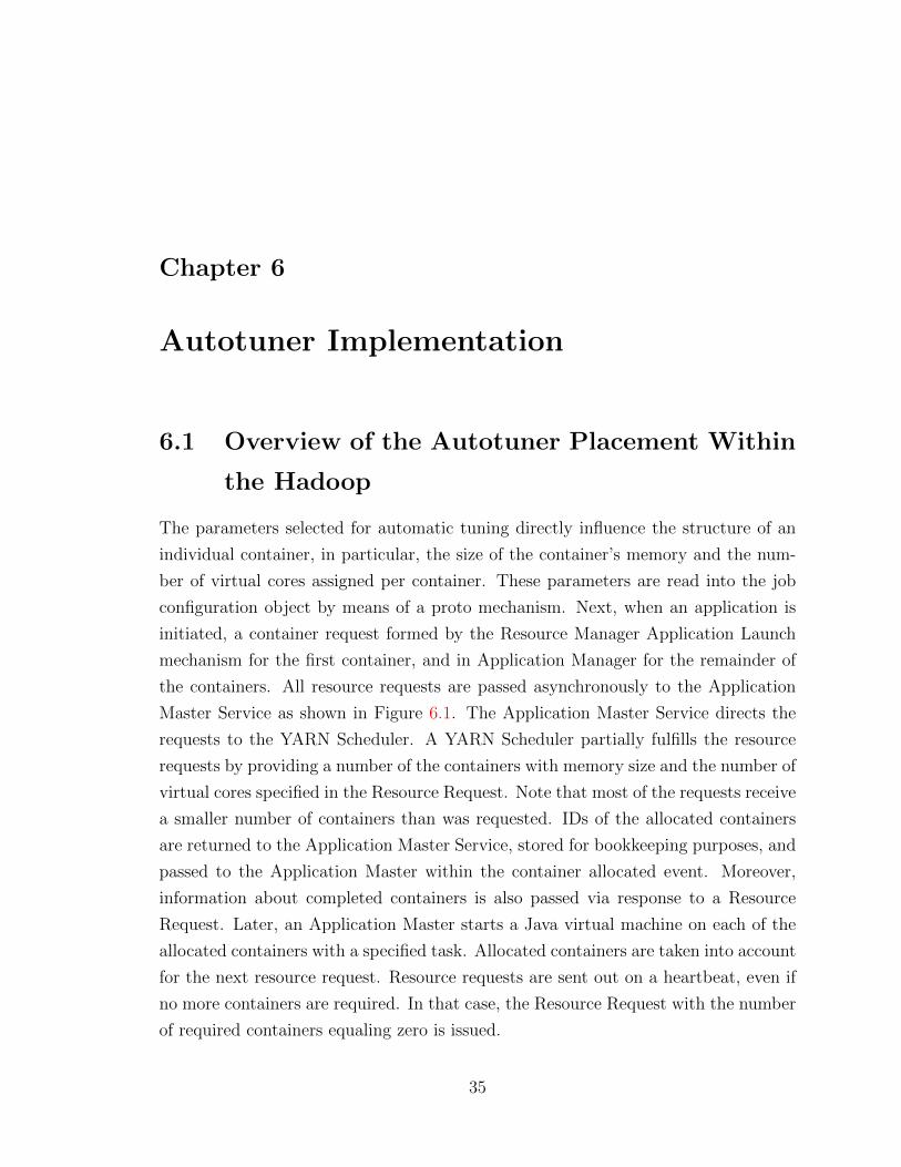
Chapter 6
Autotuner Implementation
6.1 Overview of the Autotuner Placement Within
the Hadoop
The parameters selected for automatic tuning directly influence the structure of an
individual container, in particular, the size of the container’s memory and the num-
ber of virtual cores assigned per container. These parameters are read into the job
configuration object by means of a proto mechanism. Next, when an application is
initiated, a container request formed by the Resource Manager Application Launch
mechanism for the first container, and in Application Manager for the remainder of
the containers. All resource requests are passed asynchronously to the Application
Master Service as shown in Figure 6.1. The Application Master Service directs the
requests to the YARN Scheduler. A YARN Scheduler partially fulfills the resource
requests by providing a number of the containers with memory size and the number of
virtual cores specified in the Resource Request. Note that most of the requests receive
a smaller number of containers than was requested. IDs of the allocated containers
are returned to the Application Master Service, stored for bookkeeping purposes, and
passed to the Application Master within the container allocated event. Moreover,
information about completed containers is also passed via response to a Resource
Request. Later, an Application Master starts a Java virtual machine on each of the
allocated containers with a specified task. Allocated containers are taken into account
for the next resource request. Resource requests are sent out on a heartbeat, even if
no more containers are required. In that case, the Resource Request with the number
of required containers equaling zero is issued.
35
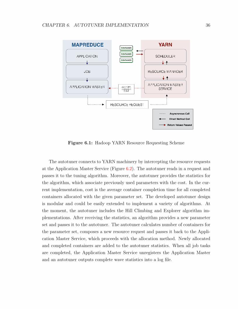
CHAPTER 6. AUTOTUNER IMPLEMENTATION 36
Figure 6.1: Hadoop YARN Resource Requesting Scheme
The autotuner connects to YARN machinery by intercepting the resource requests
at the Application Master Service (Figure 6.2). The autotuner reads in a request and
passes it to the tuning algorithm. Moreover, the autotuner provides the statistics for
the algorithm, which associate previously used parameters with the cost. In the cur-
rent implementation, cost is the average container completion time for all completed
containers allocated with the given parameter set. The developed autotuner design
is modular and could be easily extended to implement a variety of algorithms. At
the moment, the autotuner includes the Hill Climbing and Explorer algorithm im-
plementations. After receiving the statistics, an algorithm provides a new parameter
set and passes it to the autotuner. The autotuner calculates number of containers for
the parameter set, composes a new resource request and passes it back to the Appli-
cation Master Service, which proceeds with the allocation method. Newly allocated
and completed containers are added to the autotuner statistics. When all job tasks
are completed, the Application Master Service unregisters the Application Master
and an autotuner outputs complete wave statistics into a log file.
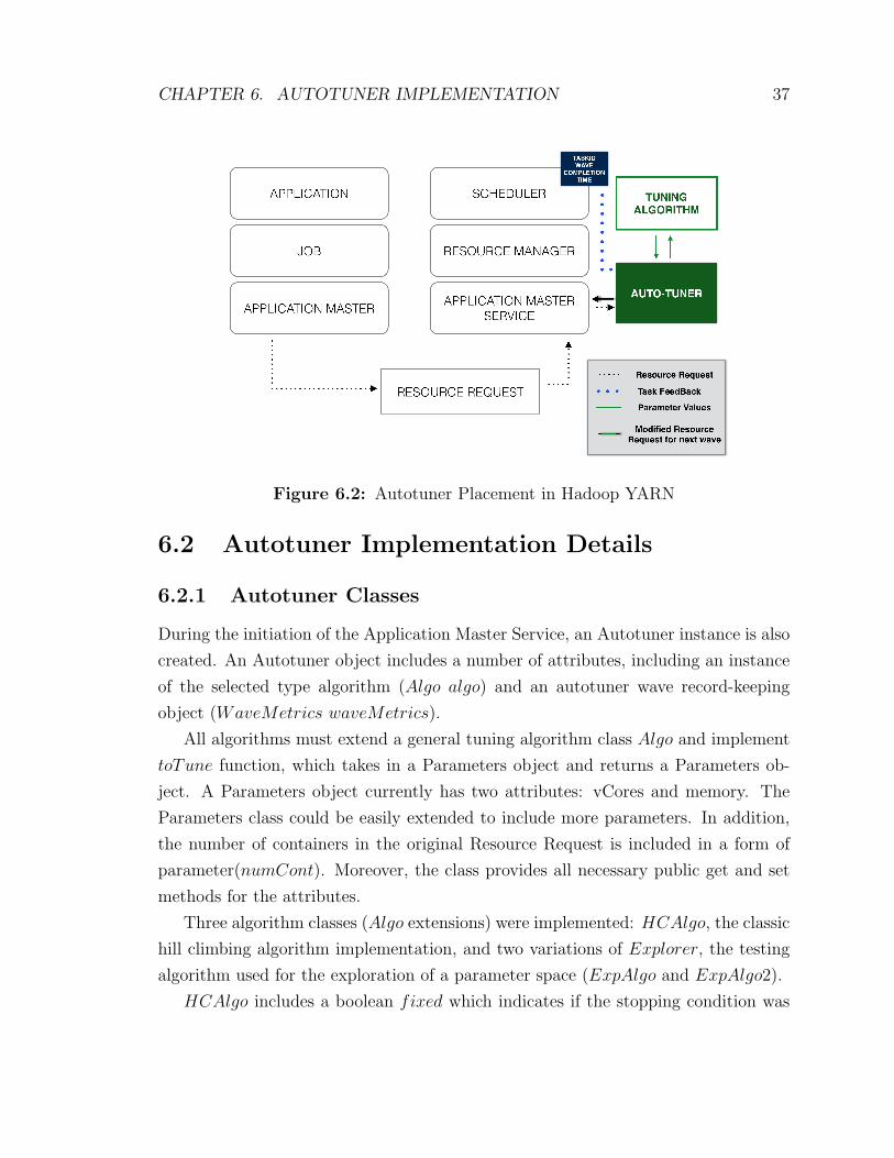
CHAPTER 6. AUTOTUNER IMPLEMENTATION 37
Figure 6.2: Autotuner Placement in Hadoop YARN
6.2 Autotuner Implementation Details
6.2.1 Autotuner Classes
During the initiation of the Application Master Service, an Autotuner instance is also
created. An Autotuner object includes a number of attributes, including an instance
of the selected type algorithm (Algo algo) and an autotuner wave record-keeping
object (WaveMetrics waveMetrics).
All algorithms must extend a general tuning algorithm class Algo and implement
toTune function, which takes in a Parameters object and returns a Parameters ob-
ject. A Parameters object currently has two attributes: vCores and memory. The
Parameters class could be easily extended to include more parameters. In addition,
the number of containers in the original Resource Request is included in a form of
parameter(numCont). Moreover, the class provides all necessary public get and set
methods for the attributes.
Three algorithm classes (Algo extensions) were implemented: HCAlgo, the classic
hill climbing algorithm implementation, and two variations of Explorer, the testing
algorithm used for the exploration of a parameter space (ExpAlgo and ExpAlgo2).
HCAlgo includes a boolean fixed which indicates if the stopping condition was
CHAPTER 6. AUTOTUNER IMPLEMENTATION 38
met. The stopping condition is the absence of a neighbour with a lower cost. Once the
stopping condition is met fixed is set to true and the Parameters object stored in
bestPar and, from this moment to the job completion, bestPar is always returned on
toTune() calls. If the fixed variable is still false, than the remaining neighbours of the
current parameters (currentPar) are explored. A new Parameter set is created by an
increase or decrease of memory or vCores and the results are stored in candidatePar.
A selection between which of the parameters will be altered, and in what direction,
is based on a random integer. Note that the parameter space has different length
dimensions, as the number of the valid virtual cores per container is much smaller than
the number of possible values for a container memory size. The Explorer algorithm
loops until all parameters within the set range are explored; it does not have a stopping
condition. An Explorer collects statistical information for each wave and outputs it
to the log file on completion of the job in the finishApplicationMaster method of
the Application Master Service.
Statistics on autotuner waves are stored in a waveMetrics object, which includes
a map, contWave of all allocated containers, ContainerIDs, a wave ID and a list of
the all created Wave objects. Each Wave object includes an integer wave ID (waveId),
and boolean newTimeAdded, which indicates if new time was added. Moreover, it
keeps track of all completed containers of the wave in a contIDs array list. The
average time of the wave (averT ime) is calculated only if it was requested and if
a new container completion time was added since the last average time calculation.
Such a ”lazy evaluation” scheme saves from unnecessary average time calculations.
Relations between autotuner waves and Hadoop waves are discussed in next section.
6.2.2 Autotuner Waves
A Hadoop wave is a collection of all containers returned as a result of a single request.
Therefore, all containers of a Hadoop wave started at the same time and have the same
memory size and number of virtual cores. A Hadoop wave is created on every Hadoop
heartbeat. Moreover, an autotuner wave collection of all containers is returned as a
result of all resource requests emitted within the same autotuner wave. An autotuner
wave is created after a set amount of time is passed, which typically includes multiple
heartbeats. An Autotuner Wave includes one or more waves initiated within a set
time period. Only full waves are included. Hence, no wave could have containers in
two separate Autotuner Waves. To illustrate the relations between the wave types
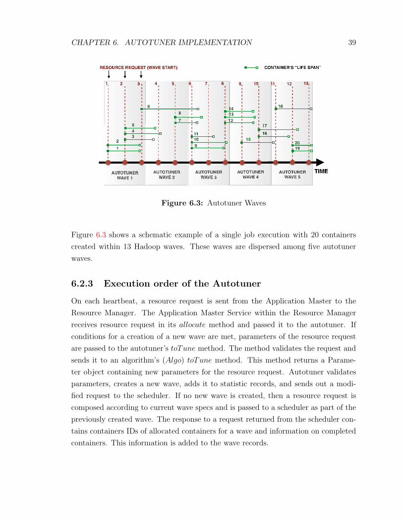
CHAPTER 6. AUTOTUNER IMPLEMENTATION 39
Figure 6.3: Autotuner Waves
Figure 6.3 shows a schematic example of a single job execution with 20 containers
created within 13 Hadoop waves. These waves are dispersed among five autotuner
waves.
6.2.3 Execution order of the Autotuner
On each heartbeat, a resource request is sent from the Application Master to the
Resource Manager. The Application Master Service within the Resource Manager
receives resource request in its allocate method and passed it to the autotuner. If
conditions for a creation of a new wave are met, parameters of the resource request
are passed to the autotuner’s toTune method. The method validates the request and
sends it to an algorithm’s (Algo) toTune method. This method returns a Parame-
ter object containing new parameters for the resource request. Autotuner validates
parameters, creates a new wave, adds it to statistic records, and sends out a modi-
fied request to the scheduler. If no new wave is created, then a resource request is
composed according to current wave specs and is passed to a scheduler as part of the
previously created wave. The response to a request returned from the scheduler con-
tains containers IDs of allocated containers for a wave and information on completed
containers. This information is added to the wave records.
CHAPTER 6. AUTOTUNER IMPLEMENTATION 40
6.2.4 Explorer
An Explorer was created to evaluate the variation between completion times of the
autotuner waves with different parameter settings. Two versions of this algorithm
were used in experiments: ExpAlgo and ExpAlgo2. Both of the versions extend the
Algo class and implement a toTune function.
ExpAlgo has an autotuner wave length of 30 seconds and considers a two dimen-
sional subspace of virtual cores (vCores) and memory. The number of virtual cores
varies between 1 and 4. Container memory ranges from 640 MB to 3200 MB and
includes 6 preset values, one of which is the default.
ExpAlgo2 has an autotuner wave length of 20 minutes and considers a one di-
mensional parameter subspace of memory. The number of virtual cores is fixed to 1.
Container memory ranges from 640 MB to 3200 MB and includes the same 6 values
as the ExpAlgo.
Chapter 7
Results
7.1 Experimental Design
Testing was completed in three different settings: default baseline, rules of thumb
baseline and auto-tuned. Testing included two baselines. The first was the execution
of TeraSort, included in the standard Hadoop distribution for 100GB and 1TB of
data. The second was the completion of TPCxP Benchmark for 1TB of data.
For the default baseline, tests were executed on ”out of the box” with default
settings for all Hadoop 2.2 parameters. For values of the important subset of pa-
rameters see Table 7.1. Rules of thumb (ROT) were collected from multiple sources.
The subset of the most important parameters, which are suitable for Hadoop 2.2
were selected and displayed in the Table 7.1. These settings were used for the rules of
thumb baseline. Finally, the third set of tests was performed on the system with ROT
values for the listed parameters changing tunables (mapreduce.map.memory.mb and
marpeduce.map.cpu.vcores from mapred− site.xml) via the autotuning mechanism.
7.1.1 Testing Cluster Configuration and Hardware
The cluster is composed of four identical machines, three of which are data nodes
(slaves) and the remaining one is a master node.
Each of the computers is empowered by Intel(R) Core(TM) i7-3770 CPU @
3.40GHz with 31GB of memory core. In addition to the 120GB INTEL solid-state
drive, which contains the operating system, it has four additional 1863GB drives,
which, all together results in a 5.37 TB storage capacity per each machine (node).
41
CHAPTER 7. RESULTS 42
7.1.2 Hadoop Cluster Settings
Configuration files were altered in a following way. First, hdfs-site.xml com-
posed of four properties: fs.defaultFS, dfs.datanode.data.dir, dfs.replication
and dfs.namenode.name.dir with hdfs://ivy23/, /hadoop2, /hadoop3, /hadoop4,
3 and /hadoop1 values, respectively. Second, core-site.xml composed of two
properties: fs.defaultFS and hadoop.tmp.dir set to hdfs : //ivy23/ and
/hadoop1/tmp values, respectively. Third, mapreduce-site.xml has a single pa-
rameter mapreduce.framework.name with value yarn. Fourth, yarn-site.xml has
three original parameters: yarn.resourcemanager.hostname is set to the mas-
ter node (ivy23 in the particular test cluster), then yarn.nodemanager.aux −services and yarn.nodemanager.aux− services.mapreduce.shuffle.class are set to
mapreduceshuffle and org.apache.hadoop.mapred.ShuffleHandler values, respec-
tively.
Additional configuration files (hadoop − policy.xml, httpfs − site.xml, kms −site.xml) remained unaltered.
7.1.3 Development environment set up with MiniYARNclus-
ter on Eclipse development environment
The configuration of the development environment itself was a nontrivial task; there-
fore, the setting up procedure presented in detail. The Hadoop 2.6 source code was
downloaded from the Hadoop official web page [12]. Next, Eclipse Platform Ver-
sion: 3.8.1 for Java Developers was installed on the Ubuntu 14.04 operating system.
Moreover, the Apache Maven 3.0.5 plugin was installed for a building process.
In order to trace the YARN Resource Manager actions, a MiniYARNCluster type
of execution must be configured. MiniYARNCluster simulates real Hadoop/YARN
cluster communication among the nodes and architectural modules by initiating mul-
tiple Java virtual machines (JVMs).
Configuration
Configuration files are found in /hadoop-2.6.0-src/hadoop-yarn-project/hadoop-
yarn/hadoop-yarn-server/hadoop-yarn-server-resourcemanager/src/test/resources.
A YARN configuration file yarn-site.xml must be modified. In particular, by default,
the configuration file does not contain any properties. A YARN configuration
CHAPTER 7. RESULTS 43
file yarn-site must be modified. Between configuration, tags must be added two
properties: yarn.nodemanager.aux − services with MapReduce shuffle value,
and yarn.nodemanager.aux − services.mapreduceshuffle.class property with
org.apache.hadoop.mapred.ShuffleHandler value.
Example file
In the example Java file before the actualMapReduce job is run, a cluster must be
set up and started and, after a MapReduce job is complete, it must be stopped. The
code must be added to the main class, before the example code. The next five steps
complete the configuration.
1. First logging should be set
Log LOG = LogFactory.getLog(WordCount.class);
LOG.info(”Starting up Mini YARN cluster);
2. Next, the new configuration is created and the MapReduce framework param-
eter is set to YARN. Moreover, additional parameters, such as minimum allo-
cation for a scheduler could be set if default values do not suffice.
Configuration conf = new Configuration();
conf.set(”mapreduce.framework.name”, ”yarn”);
conf.setInt(YarnConfiguration.RM SCHEDULER MINIMUM ALLOCATION
MB, 64);
3. After the mini cluster is initiated and started.
MiniYARNCluster miniCluster = new MiniYARNClus-
ter(”testYarnCluster”,1,1,1);
miniCluster.init(conf);
miniCluster.start();
4. It is important to create and pass to the mini cluster URL for yarn-site.xml
YARN configuration file and process the parameters that it contains.
URL url = Thread.currentThread().getContextClassLoader().getResource
(”yarn-site.xml”);
CHAPTER 7. RESULTS 44
if (url == null) {
throw new RuntimeException(”Could not find ’yarn-site.xml’ dummy file in
classpath”);
}
miniCluster.getConfig().set(”yarn.application.classpath”, new
File(url.getPath()).getParent());
OutputStream os = new FileOutputStream(new File(url.getPath()));
miniCluster.getConfig().writeXml(os);
os.close();
5. Finally, the configuration with the binding details of the created mini YARN
cluster could be obtained.
YarnConfiguration appConf = new YarnConfigura-
tion(miniCluster.getConfig());
This configuration should be passed to the app on job instantiation step. After job
completion, the mini cluster should be stopped with miniCluster.stop() method.
The example constructed following the example given above could be executed
in the development environment, such as Eclipse, by running in normal or debugger
mode. In debugger mode, breakpoints could be used in order to trace the anatomy
ofMapReduce job processing on a YARN cluster.
7.1.4 Benchmarks
Quantitative evaluation and characterization of an academic or commercial software
product through extensive benchmarking is crucial. A benchmark not only places a
compatible value on its performance but also directs development toward the most
valuable improvements. A number of benchmarks different complexity levels were
considered.
7.1.5 TeraSort Benchmark
TeraGen
TeraGen is a MapReduce program that produces a requested size file, which can be
used as an input for the TeraSort benchmark. In particular, a user specifies a number
CHAPTER 7. RESULTS 45
of rows as a command line argument and a directory for the output. Each row consists
of 100 bytes. The first 10 bytes are the key and composed of random characters from
the set ’ ’ .. ’ ’. The second 10 bytes are an integer row ID. Next 78 bytes are the
filler, which consists of seven runs of 10 characters from ’A’ to ’Z’.
TeraGen was executed from Hadoop home directory on the master node and test
data was generated.
bin/hadoopjarhadoop− examples− ∗.jarteragen10000000000/terasort− input
TeraSort
TeraSort is a traditional MapReduce benchmark, taking its roots from the tests pro-
posed in the original Google paper [5]. TeraSort is a MapReduce program, which
samples input, and produces globally sorted output of the data. TeraSort differs
from other MapReduce sorts by the custom partitioner. The partitioner utilizes
the list of N-1 sampled keys. Therefore, reducer i receives only keys in interval
[sample[i−1]; sample[i]). Hence, all keys separated in ordered ”buckets”, and output
of i-th reducer is always greater than output of (i − 1)-th. Indexing of the sample
keys is based on the first two bytes of the key and implemented as a two level trie.
Such structure speeds up the partitioning process.
Before a job is submitted, TeraSort generates the sample keys by sampling the
input. The list of sample keys is written into HDFS. Note that, the output of the
reduce has replication set to 1, instead of the default 3.
TeraGen was also executed on the data previously produced by TeraGen.
bin/hadoopjarhadoop− examples− ∗.jarterasort/terasort− input/terasort− out
TeraValidate
TeraValidate is a MapReduce program, which was developed for validation of TeraSort
output. It confirms that produced rows are in globally sorted order. Each output file
assigned to designated map task, which ensures that each key is less than or equal to
the previous one and generates records with the first and last keys of the file. Reducer
confirms that the first key of file i is greater that the last key of file (i− 1). If this is
not the case, a record is produced to the output. Therefore, an empty output signifies
that data was sorted correctly.
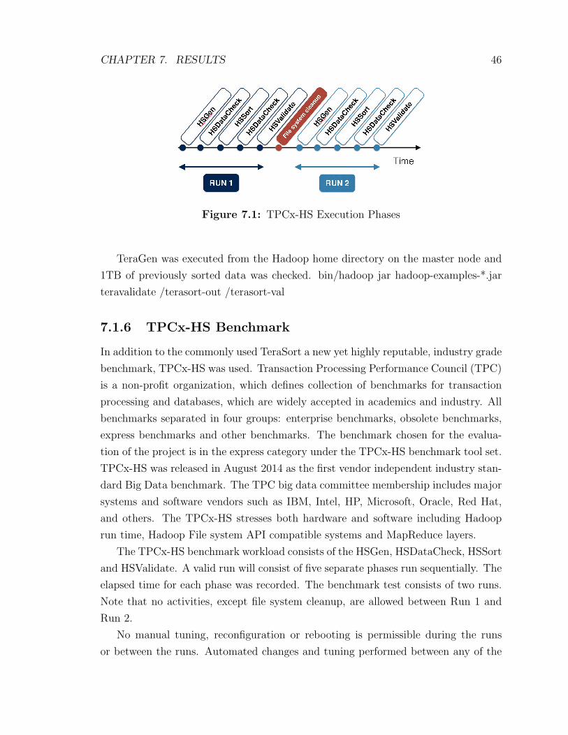
CHAPTER 7. RESULTS 46
Figure 7.1: TPCx-HS Execution Phases
TeraGen was executed from the Hadoop home directory on the master node and
1TB of previously sorted data was checked. bin/hadoop jar hadoop-examples-*.jar
teravalidate /terasort-out /terasort-val
7.1.6 TPCx-HS Benchmark
In addition to the commonly used TeraSort a new yet highly reputable, industry grade
benchmark, TPCx-HS was used. Transaction Processing Performance Council (TPC)
is a non-profit organization, which defines collection of benchmarks for transaction
processing and databases, which are widely accepted in academics and industry. All
benchmarks separated in four groups: enterprise benchmarks, obsolete benchmarks,
express benchmarks and other benchmarks. The benchmark chosen for the evalua-
tion of the project is in the express category under the TPCx-HS benchmark tool set.
TPCx-HS was released in August 2014 as the first vendor independent industry stan-
dard Big Data benchmark. The TPC big data committee membership includes major
systems and software vendors such as IBM, Intel, HP, Microsoft, Oracle, Red Hat,
and others. The TPCx-HS stresses both hardware and software including Hadoop
run time, Hadoop File system API compatible systems and MapReduce layers.
The TPCx-HS benchmark workload consists of the HSGen, HSDataCheck, HSSort
and HSValidate. A valid run will consist of five separate phases run sequentially. The
elapsed time for each phase was recorded. The benchmark test consists of two runs.
Note that no activities, except file system cleanup, are allowed between Run 1 and
Run 2.
No manual tuning, reconfiguration or rebooting is permissible during the runs
or between the runs. Automated changes and tuning performed between any of the
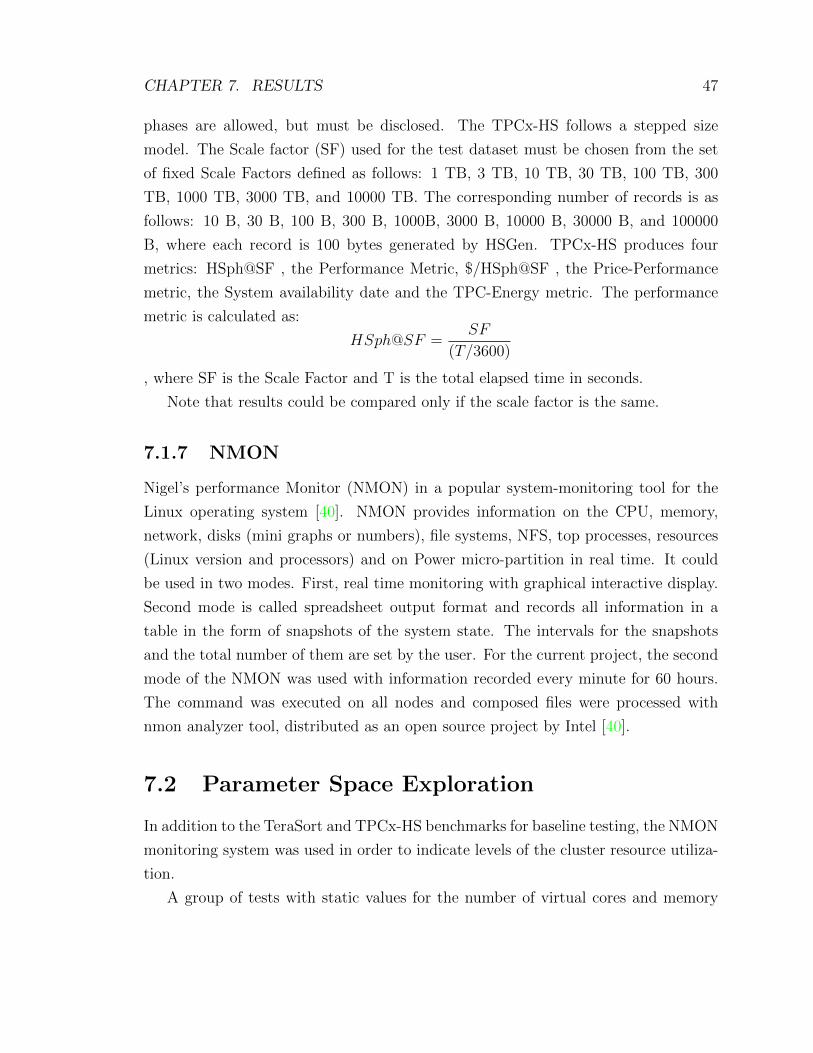
CHAPTER 7. RESULTS 47
phases are allowed, but must be disclosed. The TPCx-HS follows a stepped size
model. The Scale factor (SF) used for the test dataset must be chosen from the set
of fixed Scale Factors defined as follows: 1 TB, 3 TB, 10 TB, 30 TB, 100 TB, 300
TB, 1000 TB, 3000 TB, and 10000 TB. The corresponding number of records is as
follows: 10 B, 30 B, 100 B, 300 B, 1000B, 3000 B, 10000 B, 30000 B, and 100000
B, where each record is 100 bytes generated by HSGen. TPCx-HS produces four
metrics: HSph@SF , the Performance Metric, $/HSph@SF , the Price-Performance
metric, the System availability date and the TPC-Energy metric. The performance
metric is calculated as:
HSph@SF =SF
(T/3600)
, where SF is the Scale Factor and T is the total elapsed time in seconds.
Note that results could be compared only if the scale factor is the same.
7.1.7 NMON
Nigel’s performance Monitor (NMON) in a popular system-monitoring tool for the
Linux operating system [40]. NMON provides information on the CPU, memory,
network, disks (mini graphs or numbers), file systems, NFS, top processes, resources
(Linux version and processors) and on Power micro-partition in real time. It could
be used in two modes. First, real time monitoring with graphical interactive display.
Second mode is called spreadsheet output format and records all information in a
table in the form of snapshots of the system state. The intervals for the snapshots
and the total number of them are set by the user. For the current project, the second
mode of the NMON was used with information recorded every minute for 60 hours.
The command was executed on all nodes and composed files were processed with
nmon analyzer tool, distributed as an open source project by Intel [40].
7.2 Parameter Space Exploration
In addition to the TeraSort and TPCx-HS benchmarks for baseline testing, the NMON
monitoring system was used in order to indicate levels of the cluster resource utiliza-
tion.
A group of tests with static values for the number of virtual cores and memory
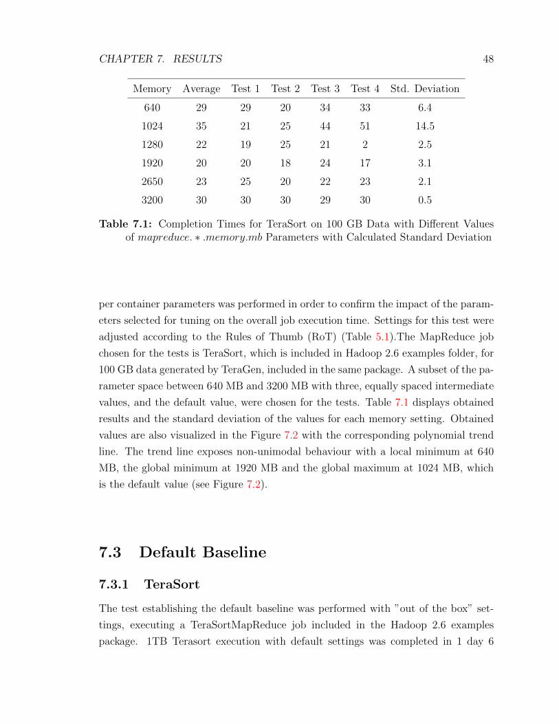
CHAPTER 7. RESULTS 48
Memory Average Test 1 Test 2 Test 3 Test 4 Std. Deviation
640 29 29 20 34 33 6.4
1024 35 21 25 44 51 14.5
1280 22 19 25 21 2 2.5
1920 20 20 18 24 17 3.1
2650 23 25 20 22 23 2.1
3200 30 30 30 29 30 0.5
Table 7.1: Completion Times for TeraSort on 100 GB Data with Different Valuesof mapreduce. ∗ .memory.mb Parameters with Calculated Standard Deviation
per container parameters was performed in order to confirm the impact of the param-
eters selected for tuning on the overall job execution time. Settings for this test were
adjusted according to the Rules of Thumb (RoT) (Table 5.1).The MapReduce job
chosen for the tests is TeraSort, which is included in Hadoop 2.6 examples folder, for
100 GB data generated by TeraGen, included in the same package. A subset of the pa-
rameter space between 640 MB and 3200 MB with three, equally spaced intermediate
values, and the default value, were chosen for the tests. Table 7.1 displays obtained
results and the standard deviation of the values for each memory setting. Obtained
values are also visualized in the Figure 7.2 with the corresponding polynomial trend
line. The trend line exposes non-unimodal behaviour with a local minimum at 640
MB, the global minimum at 1920 MB and the global maximum at 1024 MB, which
is the default value (see Figure 7.2).
7.3 Default Baseline
7.3.1 TeraSort
The test establishing the default baseline was performed with ”out of the box” set-
tings, executing a TeraSortMapReduce job included in the Hadoop 2.6 examples
package. 1TB Terasort execution with default settings was completed in 1 day 6
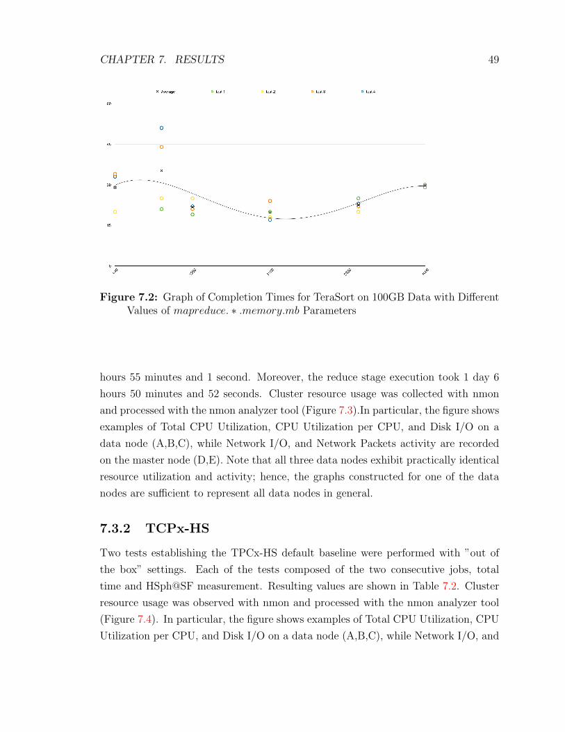
CHAPTER 7. RESULTS 49
Figure 7.2: Graph of Completion Times for TeraSort on 100GB Data with DifferentValues of mapreduce. ∗ .memory.mb Parameters
hours 55 minutes and 1 second. Moreover, the reduce stage execution took 1 day 6
hours 50 minutes and 52 seconds. Cluster resource usage was collected with nmon
and processed with the nmon analyzer tool (Figure 7.3).In particular, the figure shows
examples of Total CPU Utilization, CPU Utilization per CPU, and Disk I/O on a
data node (A,B,C), while Network I/O, and Network Packets activity are recorded
on the master node (D,E). Note that all three data nodes exhibit practically identical
resource utilization and activity; hence, the graphs constructed for one of the data
nodes are sufficient to represent all data nodes in general.
7.3.2 TCPx-HS
Two tests establishing the TPCx-HS default baseline were performed with ”out of
the box” settings. Each of the tests composed of the two consecutive jobs, total
time and HSph@SF measurement. Resulting values are shown in Table 7.2. Cluster
resource usage was observed with nmon and processed with the nmon analyzer tool
(Figure 7.4). In particular, the figure shows examples of Total CPU Utilization, CPU
Utilization per CPU, and Disk I/O on a data node (A,B,C), while Network I/O, and
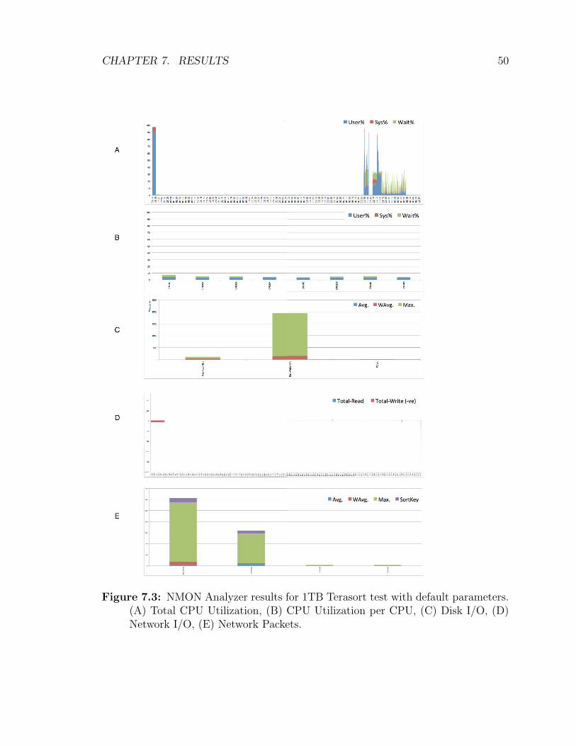
CHAPTER 7. RESULTS 50
Figure 7.3: NMON Analyzer results for 1TB Terasort test with default parameters.(A) Total CPU Utilization, (B) CPU Utilization per CPU, (C) Disk I/O, (D)Network I/O, (E) Network Packets.
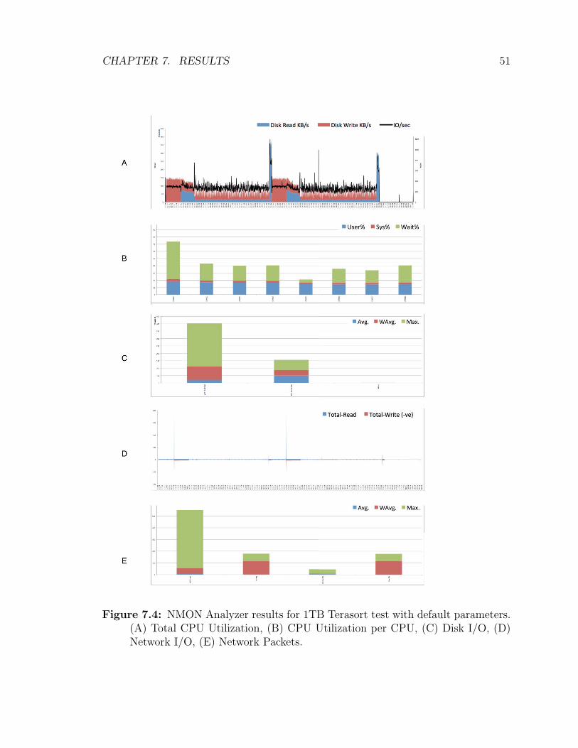
CHAPTER 7. RESULTS 51
Figure 7.4: NMON Analyzer results for 1TB Terasort test with default parameters.(A) Total CPU Utilization, (B) CPU Utilization per CPU, (C) Disk I/O, (D)Network I/O, (E) Network Packets.

CHAPTER 7. RESULTS 52
Test Run Total Time, sec HSph@SF
1 1 50658 0.0710
1 2 51541 0.0698
2 1 56267 0.0639
2 2 56306 0.0639
Table 7.2: TPCx-HS Default Baseline Tests Results
Test Total Time, ms Total Time, min
1 5855681 98
2 5528821 92
3 5810725 97
4 5897074 98
5 5612621 94
Table 7.3: TeraSort on 100GB of data with Autotuner Empowered Hadoop withHill Climbing Algorithm Tests Results
Network Packets activity are recorded on the master node (D,E).
7.4 Preliminary Autotuner Results
7.4.1 TeraSort
Testing of the Autotuner with the Hill Climbing algorithm was performed similarly
to the default baseline: TeraSort, included in the Hadoop 2.6 examples package, was
executed on 1 TB of data with default settings. The job was completed in 1 day 5
hours 49 minutes and 30 seconds.
Moreover, a series of 100 GB TeraSort tests was performed; completion times are
presented in Table 7.3.
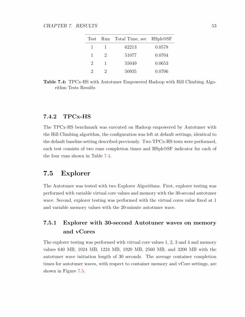
CHAPTER 7. RESULTS 53
Test Run Total Time, sec HSph@SF
1 1 62213 0.0578
1 2 51077 0.0704
2 1 55049 0.0653
2 2 50935 0.0706
Table 7.4: TPCx-HS with Autotuner Empowered Hadoop with Hill Climbing Algo-rithm Tests Results
7.4.2 TPCx-HS
The TPCx-HS benchmark was executed on Hadoop empowered by Autotuner with
the Hill Climbing algorithm, the configuration was left at default settings, identical to
the default baseline setting described previously. Two TPCx-HS tests were performed,
each test consists of two runs completion times and HSph@SF indicator for each of
the four runs shown in Table 7.4.
7.5 Explorer
The Autotuner was tested with two Explorer Algorithms. First, explorer testing was
performed with variable virtual core values and memory with the 30-second autotuner
wave. Second, explorer testing was performed with the virtual cores value fixed at 1
and variable memory values with the 20-minute autotuner wave.
7.5.1 Explorer with 30-second Autotuner waves on memory
and vCores
The explorer testing was performed with virtual core values 1, 2, 3 and 4 and memory
values 640 MB, 1024 MB, 1224 MB, 1920 MB, 2560 MB, and 3200 MB with the
autotuner wave initiation length of 30 seconds. The average container completion
times for autotuner waves, with respect to container memory and vCore settings, are
shown in Figure 7.5.
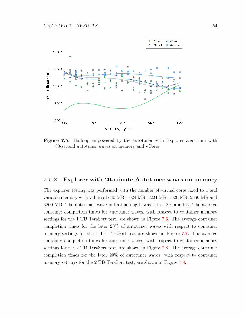
CHAPTER 7. RESULTS 54
Figure 7.5: Hadoop empowered by the autotuner with Explorer algorithm with30-second autotuner waves on memory and vCores
7.5.2 Explorer with 20-minute Autotuner waves on memory
The explorer testing was performed with the number of virtual cores fixed to 1 and
variable memory with values of 640 MB, 1024 MB, 1224 MB, 1920 MB, 2560 MB and
3200 MB. The autotuner wave initiation length was set to 20 minutes. The average
container completion times for autotuner waves, with respect to container memory
settings for the 1 TB TeraSort test, are shown in Figure 7.6. The average container
completion times for the later 20% of autotuner waves with respect to container
memory settings for the 1 TB TeraSort test are shown in Figure 7.7. The average
container completion times for autotuner waves, with respect to container memory
settings for the 2 TB TeraSort test, are shown in Figure 7.8. The average container
completion times for the later 20% of autotuner waves, with respect to container
memory settings for the 2 TB TeraSort test, are shown in Figure 7.9.
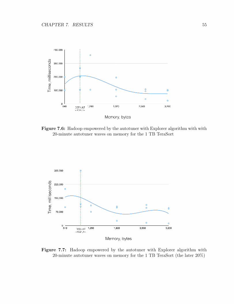
CHAPTER 7. RESULTS 55
Figure 7.6: Hadoop empowered by the autotuner with Explorer algorithm with with20-minute autotuner waves on memory for the 1 TB TeraSort
Figure 7.7: Hadoop empowered by the autotuner with Explorer algorithm with20-minute autotuner waves on memory for the 1 TB TeraSort (the later 20%)

CHAPTER 7. RESULTS 56
Figure 7.8: Hadoop empowered by the autotuner with Explorer algorithm withExplorer algorithm with 20-minute autotuner waves on memory for the 2 TBTeraSort
Figure 7.9: Hadoop empowered by the autotuner with Explorer algorithm withExplorer algorithm with 20-minute autotuner waves on memory for the 2 TBTeraSort (the later 20%)
Chapter 8
Discussion
8.1 Innovation Concept. Real-Time Autotuning
8.1.1 Rational for real-time Hadoop YARN autotuning
Hadoop exposes over 200 parameters, which drastically affect the cluster performance.
Therefore, manual tuning has to be performed to achieve the desired results. Manual
tuning is not only expensive, but also often unacceptable, because of the worldwide
shortage of Hadoop tuning experts. Large companies, associated with Big Data tech-
nology, such as IBM, have teams of professionals dedicated to provide tuning services
for the jobs run on Hadoop clusters.
Real-time autotuning is a highly desired, yet not explored problem in Hadoop
YARN tuning. Considering typical use cases in business and academia, Hadoop is
commonly deployed in situations in which the job is executed once or with a small
number of repetitions. For instance, such jobs are common in the growing field of
data science. In order to test the hypothesis on different sizes or the structure of data,
optimal settings are different for every single execution must be tuned individually.
Therefore, running the same job multiple times in order to obtain optimal param-
eter settings, even though it makes the single execution faster, overall, it makes it
a few folds slower than the time achieved at default settings. Notice, that this will
be the case in all off-line tuning algorithms, including the genetic algorithm, simu-
lated annealing and hill climbing described earlier. For instance, the Gunther project
employs a genetic algorithm, and produces optimal completion time under 12 genera-
tions. The obtained completion time was two times faster than original. Each of the
generations must have taken at least optimal time. Therefore, to complete tuning,
57
CHAPTER 8. DISCUSSION 58
Gunther took 12 times the optimal job completion time or 6 times the worst (original)
time. Hence, for the use cases in which a job is run under 6 times, the employment
of Gunther could not be justified. All other off-line autotuners follow the same logic,
which makes them not practical for the most popular Hadoop use cases. Therefore,
real-time Hadoop YARN autotuning is a worthwhile and desirable research aim.
8.1.2 Autotuner Design Requirements
From the use cases mentioned earlier, desirable specifications for the autotuner archi-
tecture and functionality were derived. First and foremost, it was established that,
for the most common Hadoop use cases, the total autotuning process should not take
more than a single run on default settings. Therefore, an automatic tuning process
must execute during a single Hadoop job.
In case of off-line autotuning, the cost function is based on information (such as
completion time) obtained at the end of the job execution. Hence, the completion of
the tuning within a time frame of a single default run is unfeasible. Therefore, a cost
function must be developed, which estimates the total job completion time based on
the information collected on a part of the job.
Furthermore, in order to on-line tune the parameters within the job execution,
the autotuner must intercept tunables, collect cost evaluation, process information,
produce new values for tunables and substitute old values with the new during exe-
cution on the Hadoop job. Therefore, the tuner must be tightly coupled with Hadoop
YARN architecture, yet not interfere with the job flow. For instance, the autotuning
process must be fast, in order to avoid lengthening the Hadoop job execution.
Moreover, it is desirable for the autotuner to be modular, with multiple algorithm
options. Hence, a user can evaluate different tuning techniques employing the same
real-time parameter changing mechanism.
8.2 Design Decisions Motivation
During the software design and implementation processes, a number of important
design decisions were made. Let us review the most significant of the decisions in
the current section. First, we will look at the rationale behind the selection of the
tunables. Second, we will look at the point at which the Hadoop job flow must be
CHAPTER 8. DISCUSSION 59
accessed and modified. Third, we will look at the main modules of the autotuner and
which tuning algorithms should be included in the initial prototype.
The selection of the tunables was based on two main factors: research of the pub-
lished recommendations on Hadoop configuration tuning, and preliminary testing.
Research of the potential tunables, which have sufficient impact on performance for
MapReduce jobs on Hadoop/YARN architecture and applicable for real-time tuning
was conducted. First, the full list of the parameters recommended to be tuned to
optimize performance from various sources was compiled. Note that because of a
recent transition to YARN-based architecture many previously important parame-
ters became depreciated, or lost their effect on the system. Hence, the parameters
were filtered accordingly. Next, a subset of parameters suitable for real-time tuning
was selected and the most influential of the parameters were considered. Finally, a
preliminary review of Hadoop/YARN architecture allowed us to select two sets of pa-
rameters, which were considered for the current research: mapreduce. ∗ .memory.mb
and mapreduce. ∗ .cpu.vcores, where * stands for map and reduce. Commonly, map
and reduce types of the parameters are set to the same value. Hence, for the current
stage of the research, the map and reduce parameters were tuned to the same value.
The selected parameters are specific to YARN-based Hadoop architecture and govern
the size of memory and the number of virtual cores assigned to individual containers
by the resource manager during the resource allocation process. Overall, the pa-
rameters allow indirect control of container granularity and density; therefore, they
are affecting job completion time through the optimization of the cluster resource
deployment.
In order to confirm that the parameters selected for the tuning have an impact
and create non-trivial parameter space, a series of tests on a subset of parame-
ter space was performed. A number of TeraSort jobs were executed with differ-
ent mapreduce.map.memory.mb and mapreduce.reduce.memory.mb in configuration
files. Completion times of the experiments are plotted against parameter values re-
vealing multiple local minimum and maximum with default parameter been the global
maximum (Figure 7.2 ). Such results suggest that the selected parameters are indeed
the suitable subject for the tuning application.
The selected parameters are read from a mapred− site.xml configuration file and
added to the job configuration object. Later, a job process uses it to calculate the
complete set of containers required to complete the application. For MapReduce type
CHAPTER 8. DISCUSSION 60
jobs, containers are differentiated by the type of the task (map or reduce). Other types
of jobs executed on the YARN base have homogeneous containers. In either case, the
container configuration is passed to the resource manager via resource request. Each
request is composed of the total number of containers needed to complete the job and
amount of memory and virtual cores required per container. The Resource Request is
updated and resent on every heartbeat. Two options were considered. The first option
is to change the job configuration and create an additional mechanism, which would
force an Application Master to recalculate the Resource Request based on the new
set of container parameters. The second option is to interfere with already composed
resource requests before their fulfillment, then change the values of the requested
container memory and virtual cores. After careful consideration, which included
Hadoop and YARN code investigation, understanding overall architecture intentions
and dependencies, the second option was chosen. The modification of a Resource
Request achieves the desired effects with the least amount of interference with the
native Hadoop code without imposing an additional cycle. Resource Requests are sent
repetitively based on the heartbeats, which orchestrate most of the processes accruing
in Hadoop Yarn architecture. Therefore, employment of the heartbeat mechanism for
the real-time autotuning processes is highly desirable.
Next, the decision was to select a place in a resource passing sequence for the
autotuning interference. The interception could be done at an Application Master,
before each request is sent; at the Resource Manager’s Application Master Service,
which governs container allocation calls validation; or at a YARN Scheduler, where a
Resource Request is fulfilled. Note that a Resource Request is passed asynchronously
between the Application Master and YARN site with the Resource Manager, which
contains both an Application Master Service and Schedulers. Therefore, implementa-
tion on the YARN site allows the future extension of the Autotuner from the MapRe-
duce to the wide range of other YARN-based applications. Moreover, YARN-based
Resource Request interception is directly traceable and could be tested within the
development environment on a Mini YARN Cluster. On the YARN site, both op-
tions, an Application Master Service and a Scheduler, were considered equally valid.
Nevertheless, the main autotuner connection was chosen to be implemented on the
base Application Master Service class as the autotuner purpose is in tighter agreement
with the main roles of the Application Master Service class in the YARN architecture.
Even though the autotuner was built with modularity as the key design principle

CHAPTER 8. DISCUSSION 61
Figure 8.1: Comparison of the trend-lines: (A) Complete Terasort execution times,(B) Average container completion time per the autotuner wave during 1TBTerasort, (C) Average container completion time per the autotuner wave during2TB Terasort
and, in future selection among multiple algorithms, is extremely desirable at this
stage, one algorithm must be selected to limit the scope of the current project to a
manageable size. A number of popular algorithms used for non-unimodal parameter
space tuning were considered including genetic, simulated annealing and hill climbing
algorithms. A hill climbing algorithm was chosen for its simplicity and absence of
additional parameters, which would create additional tunables for the user.

CHAPTER 8. DISCUSSION 62
8.3 Result Evaluation
8.3.1 Comparison of the Preliminary Autotuner Runs with
Default and RoT Testings
The comparison of the trend-lines was produced by plotting multiple complete
Hadoop Terasort executions completion times against the memory parameter value
(Figure 8.1 (A)) and trend-lines produced by the average container completion time
per the autotuner wave against container memory size value for the wave for Tera-
sort Executions on 1 TB and 2 TB of data (Figure 8.1 (B),(C)). Note Figure 8.1
combines Figures 7.2, 7.6, 7.7, 7.8, and 7.9 in order to expose striking similarity in
trend-line shapes. The difference in scales between complete job executions and the
average wave container completion times prevents from joining all graphs in one.
Nevertheless, analogous behaviour of all trend-lines is unquestionable. Moreover, the
exclusion of first 80% of containers, in order to illuminate possibility of the effects
carried from the previous waves. The graph comparison shows that the illumination
of the earlier containers positively effects the 1 TB execution, yet has no effect on
the 2 TB Terasort execution trend-lines. Hence, scheduling mechanisms, in some
cases, prevent clear separation among the waves and the previous wave could affect
completion of the first containers of the wave. This could be addressed by providing
an autotuner-specific YARN Scheduler, which could provide better wave segregation.
8.3.2 Explanation of the Results Obtained by Preliminary
Autotuner Testing and Explorer Execution
One of the valid explanations for the absence of the improvement is a problem with
the implementation mechanism or with cost function. For example, the additional
time the autotuner takes to calculate a new set of parameters and pass them to the
Application Master Service is excessive. In order to test the hypothesis, time stamps
were taken before and after the autotuner is called to tune. The result shows on
average 3 ms per the autotuner wave. Hence, the time that autotuner adds to the
overall execution is marginal and cannot explain the behaviour.
The next hypothesis is that the altering Resource Request is not a sufficient mech-
anism to alter the container size during job execution. Moreover, the cost function

CHAPTER 8. DISCUSSION 63
is based on the average container completion time of the wave, which could be in-
effective. In order to validate the two hypothesis, an explorer test was performed.
First, with 30-second and 1-minute lengths of the wave, both show high variation in
container completion times within the waves set to the same memory and the num-
ber of virtual cores per container. The results shown in Figure 8.1 did not exhibit a
correlation between variation in full job run completion times and average container
completion time; yet, the result cannot be considered final as multiple additional rea-
sons could be playing a part in the outcome. For example, waves are not long enough
to clear the queue; hence, containers from previous waves temporally overlap, the
current wave containers creating excessive noise in the data. From this observation,
an idea to elongate wave lengths was derived. Moreover, data have shown that, in all
testings, the number of the virtual cores directly correlates with container completion
time. Therefore, the best time is always exhibited by the vCores parameter set to
one. In order to obtain more readable results, new explorer testing was performed
with the vCores parameter fixed to a single core and a wave length of 20 minutes.
Obtained results for Terasort on 1TB and 2TB of data were plotted as is shown
in Figure 7.6,7.8 and directly correspond to the trend line obtained for the full job
executions, which is displayed in Figure 8.1. This result not only strongly supports
the cost function, but also confirms the effectiveness of the autotuner implementation
mechanism, as the resulting autotuner wave time directly correlates with the full job
completion time.
Moreover, the observed variation in average container completion times could
serve as a sufficient explanation of autotuner inefficiency in the current state. A hill
climbing algorithm has very little chance to work towards improvement given the
size of the improvement and the range of the fluctuation among the values for the
same parameter settings. As it clearly shows in Figure 7.2, starting at the default
value, even though, on average, default is the worst performing setting, there is a
great chance that the hill climbing algorithm will not find a better neighbour and
sets there. Hence, complete execution will be performed with the default settings.
Therefore, in order to achieve effective improvement in completion times, the level of
noise in the completion times must be lowered.
CHAPTER 8. DISCUSSION 64
8.3.3 Strength of the Current Autotuner Design
As a result of this work, the autotuner implementation was developed, which not only
works, but also works efficiently. Considering how short the time that autotuner takes
in comparison to the total job time, it practically does not impose any additional cost
to run.
Moreover, it includes an accurate cost function, which correctly estimates the
complete job running time based on a test (autotuner wave) performed on a small
portion of the job. The accuracy of the evaluation confirmed with explorer tests is
summarized in Figure 8.1.
Moreover, the Autotuner was placed strategically among the YARN architecture
and localized within the Resource Manager package. Hence, deployment of the Au-
totuner is extremely simple even on an existent Hadoop cluster.
The modularity of the Autotuner design allows for easy extensions with additional
algorithms via a simple inheritance mechanism. For example, multiple algorithm
classes could be implemented as extensions of Algo. Moreover, additional parameters
could be tuned and could simply be added to the Parameters object.
Furthermore, the steps towards the understanding of observed variation among
the data points was taken. A group of hypotheses was considered. First, such varia-
tion could be triggered by a wave influences extended to the next wave for some period
of time. In particular, it reflects how the scheduler propagates the Resource Request
configuration to the actual resource allocation. As a scheduler does not implement
changes unless currently running, containers complete their tasks and a scheduler
queue is repopulated with containers with new memory and virtual core number set-
tings. Hence, in order to test this hypothesis, Explorer test data was filtered, which
excluded containers influenced by a previous wave (only last 20% of the container
were taken into account). Such a measure must exclude containers influenced by a
previous wave. Results show that only the smaller job (Terasort on 1TB of data)
with less data points produces a slightly improved trend line, which more closely
corresponds to the complete job execution parameter exploration graph (see Figures
7.7). Nevertheless, the larger job (2TB Terasort) did not exhibit significant changes
in trend line behaviour. Moreover, graphs created by complete container data and by
the last 20% of the containers are almost identical (see Figures 7.9). Hence, the auto-
tuning mechanism is not significantly influenced by the temporal overlapping between
waves created by the scheduler implementation, especially for larger workloads.
CHAPTER 8. DISCUSSION 65
8.3.4 Weakness of the Current Autotuner Design and Ideas
for Improvement
Currently no significant improvement of the map reduce runs on Hadoop 2.2 with
YARN was observed. As was previously discussed, a number of factors could be
the reason, or a part of the reason, for such a result. It was determined that the
parameters selected for tuning have an impact on the job run time and that the
mechanism for parameter changing in real-time is effectively changes parameters and
receives corresponding evaluation. Hence, the inefficiency of the autotuner must take
root in the tuning algorithm and the specifics of the data. In particular, observed high
variation for each memory setting, especially in relation with achievable improvement,
creates a low probability for a hill climbing algorithm to improve the current state.
Hence, improvement could be achieved by gaining insight on causes of the variation
and lowering its levels. The possible reasons for such behaviour could be divided in
two classes: software related and hardware related. Hardware related variation is
based on the fact that testing cluster is composed of only four nodes, and only three
of them carry actual computation as data nodes. Therefore, any inconsistencies in
performance, partial or complete failures have a considerable impact on performance,
despite the renowned Hadoop robustness.
Next, software related reasons caused by the excessive variance should be consid-
ered. Hadoop and YARN compose complex software framework, which could conceal
multiple reasons for such behaviour. For example, taking into account the slight trend
line improvement for a smaller job that exclusion of the first 80% of container com-
pletion times weighted average scheme or more custom tailored for the work with the
Autotuner YARN scheduler could be considered. Such implementation can reduce
variance among the waves.
In addition, the variation between container completion times could be triggered
by the heterogeneity of the tasks completed by individual containers. In particular,
a few individual containers of the MapReduce job seem to be running up to ten fold
longer than an average container. Moreover, map and reduce tasks could require dif-
ferent settings. Therefore, the autotuner could benefit from the delayed start and two
mode tuning, which differentiates between containers produced for map and reduce
tasks.
Moreover, extending rules of thumb selection to a wider range of parameter may
help stabilize container completion time variation. Nevertheless, similar variations in

CHAPTER 8. DISCUSSION 66
the total job completion times for the original Hadoop installation strongly suggest
that roots of the observed noise lay outside of the autotuner, and must be addressed
on the cluster level.
Chapter 9
Summary
9.1 Overview of the Results
Current work emphasizes the importance of real-time automatic tuning method
and proves the existence of a mechanism for utilization of the idea on the current
Hadoop/YARN architecture.
A novel real-time autotuning approach for MapReduce jobs executed on
Hadoop/YARN framework was proposed and implemented. The autotuner imple-
mentation connected to Hadoop/YARN through the Resource Manager and was built
in a modular, extendable manner. The parameters, responsible for configuration of
individual containers, were tuned between execution waves by the autotuner. The
effectiveness of the autotuner’s method of Resource Request interception and mod-
ification was experimentally proven. Moreover, a valid cost evaluating function was
developed.
Furthermore, initial autotuner test results were evaluated and steps toward dis-
closure of the issues preventing the autotuner from fulfillment of its objectives were
made. Moreover, a road map of further development for the autotuner composed of
prioritized items in the desired order was composed.
67
CHAPTER 9. SUMMARY 68
9.2 Future Development
The developed autotuner is the basis for a much larger project. The road map of
the future development could be divided in a number of steps. Such steps form an
agenda of goals, which should be executed in order. All steps could be divided in
three groups based on priority.
The first group of the future development is the most critical. It includes steps
that will bring the autotuner to the minimal pragmatically compelling state. First,
the source of the noise must be found. A number of hypotheses should be tested. For
instance, if noise is a result of the small cluster size and hardware state, then a test
on a larger cluster will show more stable results. Another reason for the noise could
be the dual nature of a MapReduce job. Containers with the same parameters could
not only run map and reduce tasks with different speeds, but also react differently
on parameter changes. For example, an increase in memory at some point could
speedup map containers, but slow down reduce tasks, creating the noise. To test this
hypothesis, the job composed from map or reduce tasks only should be run, such as
TeraGen, for example.
Next, when the source of variation is found, noise should be reduced to the level
accepted by the tuning algorithms. This step will depend on the source nature. For
example, in a case of hardware dependence, recommendations for a minimal size of a
cluster, on which the autotuner should be employed, could be made. In case of map
and reduce task differences, causation for the noise, implementation of two phase
tuning mechanisms and individual for each of a task type could be considered.
The second group of future developments expands the autotuner project. A num-
ber of autotuning algorithms could be increased. Moreover, an existing hill climbing
algorithm could be improved using successful techniques such as the Late Acceptance
Hill Climbing algorithm. Next, an autotuner-specific scheduler could be built, in or-
der to propagate tuning to another level. Moreover, a number of parameters selected
for real-time, automatic tuning could be increased. Another way of improving the
autotuner could be increased, coupling real-time automatic tuning with a system of
rule-based tuning, which converts out of the box default configuration to the one
closer to a rule-of-thumb tuned state before a job execution process. Cost evaluating
function should take into account not only container completion time, but also the
overall structure of the cluster resources employment in order to minimize idle state.
The third group of future development addresses the deployment process. It

CHAPTER 9. SUMMARY 69
includes an addition of a simple user interface and a parameterization of some of
the currently fixed values, such as algorithm selection, or the autotuner wave length.
Creation of Hadoop patch. Moreover, making the autotuner available for installation
on top of the current Apache Hadoop should be set as the final goal of the project.
Encapsulating the significance of the work undertaken within this project the
extensive scope and enormous practical value of the final goal must be acknowledged.
This project laid a strong base for farther advancement towards the goal.
List of References
[1] T. O. E. Dictionary, “Big data.”
[2] D. Laney, “3d data management: controlling data volume, velocity and vari-ety. meta group, ht tp,” blogs. gartner. com/doug-laney/files/2012/01/ad949-3D-Data-Management-Controlling-Data-Volume-Velocity-and-Variety. pdf (accessed16 January 2013), 2001.
[3] T. H. Davenport and D. Patil, “Data scientist: The sexiest job of the 21stcentury-a new breed of professional holds the key to capitalizing on big dataopportunities. but these specialists aren’t easy to findand the competition forthem is fierce.,” Harvard Business Review, p. 70, 2012.
[4] J. Dean and S. Ghemawat, “Map-reduce: Simplified data processing on largeclusters,” D OSDI IEEE, 2004.
[5] J. Dean and S. Ghemawat, “Mapreduce: simplified data processing on largeclusters,” Communications of the ACM, vol. 51, no. 1, pp. 107–113, 2003.
[6] S. Ghemawat, H. Gobioff, and S.-T. Leung, “The google file system,” in ACMSIGOPS operating systems review, vol. 37, pp. 29–43, ACM, 2003.
[7] I. D. Corporation, “Idc releases first worldwide hadoop-mapreduce ecosystemsoftware forecast, strong growth will continue to accelerate as talent and toolsdevelop,” 2012.
[8] H. Herodotou, H. Lim, G. Luo, N. Borisov, L. Dong, F. B. Cetin, and S. Babu,“Starfish: A self-tuning system for big data analytics.,” in CIDR, vol. 11,pp. 261–272, 2011.
[9] H. Herodotou and S. Babu, “Profiling, what-if analysis, and cost-based optimiza-tion of mapreduce programs,” Proc. of the VLDB Endowment, vol. 4, no. 11,pp. 1111–1122, 2011.
[10] G. Liao, K. Datta, and T. L. Willke, “Gunther: search-based auto-tuning ofmapreduce,” in Euro-Par 2013 Parallel Processing, pp. 406–419, Springer, 2013.
[11] Y. Chen, M. Winslett, Y. Cho, and S. Kuo, “Automatic parallel i/o performanceoptimization in panda,” in Proceedings of the tenth annual ACM symposium onParallel algorithms and architectures, pp. 108–118, ACM, 1998.
70
71
[12] A. Bialecki, M. Cafarella, D. Cutting, and O. OMalley, “Hadoop: a frameworkfor running applications on large clusters built of commodity hardware, 2005,”Wiki at http://lucene. apache. org/hadoop, 2005.
[13] M. Zaharia, M. Chowdhury, M. J. Franklin, S. Shenker, and I. Stoica, “Spark:cluster computing with working sets,” in Proceedings of the 2nd USENIX con-ference on Hot topics in cloud computing, vol. 10, p. 10, 2010.
[14] P. Mundkur, V. Tuulos, and J. Flatow, “Disco: a computing platform for large-scale data analytics,” in Proceedings of the 10th ACM SIGPLAN workshop onErlang, pp. 84–89, ACM, 2011.
[15] S. Plimpton and K. Devine, “Mapreduce-mpi library,” Sandia National Labo-ratories. Available fr om http://www. sandia. gov/˜ sjplimp/mapreduce. html,accessed on March, vol. 4, 2013.
[16] E. Dede, Z. Fadika, J. Hartog, M. Govindaraju, L. Ramakrishnan, D. Gunter,and R. Canon, “Marissa: Mapreduce implementation for streaming science ap-plications,” in E-Science (e-Science), 2012 IEEE 8th International Conferenceon, pp. 1–8, IEEE, 2012.
[17] R. M. Yoo, A. Romano, and C. Kozyrakis, “Phoenix rebirth: Scalable mapreduceon a large-scale shared-memory system,” in Workload Characterization, 2009.IISWC 2009. IEEE International Symposium on, pp. 198–207, IEEE, 2009.
[18] A. S. Foundation, “Determine yarn and mapreduce memory configuration set-tings,” 2014.
[19] A. S. Foundation, “Determine yarn and mapreduce memory configuration set-tings,” 2014.
[20] C. A. Schaefer, V. Pankratius, and W. F. Tichy, “Atune-il: An instrumenta-tion language for auto-tuning parallel applications,” in Euro-Par 2009 ParallelProcessing, pp. 9–20, Springer, 2009.
[21] M. J. Cafarella and C. Re, “Manimal: relational optimization for data-intensiveprograms,” in Procceedings of the 13th International Workshop on the Web andDatabases, p. 10, ACM, 2010.
[22] N. Yigitbasi, T. L. Willke, G. Liao, and D. Epema, “Towards machine learning-based auto-tuning of mapreduce,” in Modeling, Analysis & Simulation of Com-puter and Telecommunication Systems (MASCOTS), 2013 IEEE 21st Interna-tional Symposium on, pp. 11–20, IEEE, 2013.
[23] T. Lipcon, “Cloudera: 7 tips for improving mapreduce performance,” 2009.
[24] T. Lipcon, “Cloudera: Optimizing mapreduce job performance,” 2012.
[25] Impetus, “Hadoop performance tuning,” 2012.
72
[26] B. Behzad, S. Byna, S. M. Wild, M. Prabhat, and M. Snir, “Improving paralleli/o autotuning with performance modeling,” in Proceedings of the 23rd Inter-national Symposium on High-performance Parallel and Distributed Computing,HPDC ’14, (New York, NY, USA), pp. 253–256, ACM, 2014.
[27] J. Liu, N. Ravi, S. Chakradhar, and M. Kandemir, “Panacea: towards holisticoptimization of mapreduce applications,” in Proceedings of the Tenth Interna-tional Symposium on Code Generation and Optimization, pp. 33–43, ACM, 2012.
[28] Q. Chen, M. Guo, Q. Deng, L. Zheng, S. Guo, and Y. Shen, “Hat: history-based auto-tuning mapreduce in heterogeneous environments,” The Journal ofSupercomputing, vol. 64, no. 3, pp. 1038–1054, 2013.
[29] E. R. Lucas Filho, E. C. De Almeida, Y. Le Traon, et al., “Intra-query adaptivityfor mapreduce query processing systems,” in IDEAS 2014: 18th InternationalDatabase Engineering & Applications Symposium, 2014.
[30] M. Li, L. Zeng, S. Meng, J. Tan, L. Zhang, A. R. Butt, and N. Fuller, “Mronline:Mapreduce online performance tuning,” in Proceedings of the 23rd internationalsymposium on High-performance parallel and distributed computing, pp. 165–176,ACM, 2014.
[31] S. Kirkpatrick, C. D. Gelatt, M. P. Vecchi, et al., “Optimization by simulatedannealing,” science, vol. 220, no. 4598, pp. 671–680, 1983.
[32] V. Cerny, “Thermodynamical approach to the traveling salesman problem: Anefficient simulation algorithm,” Journal of optimization theory and applications,vol. 45, no. 1, pp. 41–51, 1985.
[33] A. M. Turing, “Computing machinery and intelligence,” Mind, pp. 433–460,1950.
[34] N. A. Barricelli, “On the manner in which crossbreeding takes place in bacterio-phages and bacteria,” Acta Biotheoretica, vol. 11, no. 2, pp. 75–84, 1955.
[35] B. Behzad, H. V. T. Luu, J. Huchette, S. Byna, R. Aydt, Q. Koziol, M. Snir,et al., “Taming parallel i/o complexity with auto-tuning,” in Proceedings of theInternational Conference on High Performance Computing, Networking, Storageand Analysis, p. 68, ACM, 2013.
[36] B. Selman and H. Kautz, “Domain-independent extensions to gsat: Solving largestructured satisfiability problems,” in IJCAI, vol. 93, pp. 290–295, Citeseer, 1993.
[37] E. K. Burke and Y. Bykov, “The late acceptance hill-climbing heuristic,” Uni-versity of Stirling, Tech. Rep, 2012.
[38] A. S. Foundation, “Hadoop mapreduce next generation - cluster setup,” 2014.
[39] Hortonworks, “Determine yarn and mapreduce memory configuration settings,”2014.
[40] IBM, “nmon,” 2013.
Appendix A
The List of Imports for a
MiniYARNCluster
• java.io.IOException;
• java.util.StringTokenizer;
• org.apache.hadoop.conf.Configuration;
• org.apache.hadoop.fs.Path;
• org.apache.hadoop.io.IntWritable;
• org.apache.hadoop.io.Text;
• org.apache.hadoop.mapreduce.Job;
• org.apache.hadoop.mapreduce.Mapper;
• org.apache.hadoop.mapreduce.Reducer;
• org.apache.hadoop.mapreduce.lib.input.FileInputFormat;
• org.apache.hadoop.mapreduce.lib.output.FileOutputFormat;
• org.apache.hadoop.util.GenericOptionsParser;
• org.apache.hadoop.yarn.conf.YarnConfiguration;
• org.apache.hadoop.yarn.server.MiniYARNCluster;
• org.apache.hadoop.yarn.server.resourcemanager.scheduler.ResourceScheduler;
73

APPENDIX A. THE LIST OF IMPORTS FOR A MINIYARNCLUSTER 74
• org.apache.hadoop.yarn.server.resourcemanager.scheduler.fifo.FifoScheduler;
• java.io.File;
• java.io.FileOutputStream;
• java.io.OutputStream;
• java.net.URL;
• org.apache.commons.logging.Log;
• org.apache.commons.logging.LogFactory;

![BigData and MapReduce with Hadooppluton.ijs.si/CLASS/files/KC_CLASS_IJS_Tomasic_2012.pdf · Hadoop Distributed File System (HDFS), Hadoop YARN and Hadoop MapReduce [2]. At the beginning](https://img.pdfslide.net/doc/110x75/5ec563644764cc6aa33a44d1/bigdata-and-mapreduce-with-hadoop-distributed-file-system-hdfs-hadoop-yarn-and.jpg)