Embed Size (px)
Citation preview

Real-time
Background Cut
Alon Rubin Shira Kritchman
Present:
7.5.2006, Weizmann Institute of Science

The Challenge
Real-time bilayer segmentation of video

The Challenge
• Real-time bilayer segmentation of video
– Fully automatic
– High quality
– Robustness to changing background
– And yet – efficient!
Application
Background substitution in video conferencing
• Privacy
•Coolness

Example

Overview
• General method
• 2 binocular (stereo) algorithms
• 2 monocular algorithms

How to Segment?

How to Segment?
• Information
– Colour
– Contrast
– Disparity
– Motion

How to Segment?
• Information
• Prior assumptions
– Spatial coherence
– Temporal coherence

• Information
• Prior assumptions
How to Segment? Notation
• - point in a 3D colour space
• - segmentation label
• - set of neighbours
rI
BFxr ,
C
F/B
),( sr
r sr

Combining Cues
Need: mathematical formulation• Prior assumptions
– Spatial coherence
– Temporal coherence
– Priors over disparity
• Informative cues
– Colour
– Contrast
– Stereo
– Motion
)|(log)(log)|(log)( xIxIxx pppE
||)||exp(*sr IIV
)|,(log),,( IdxxdI pE
0dd ),|()( Br
BrrrB INIp
ff tt 3
),,ˆ,,(minargˆ 21 tttttt E mIxxxIx
1.0
?

Prior
Combining Cues
• Probabilistic framework:
– Maximizing
• Bayes’ law:
• Gibbs energy
– Maximizing probability Minimizing energy
– Dynamic programming / Graph cut
)|( Ixp
)|(log)(log)|(log)( xIxIxx pppE
)|()()|( xIxIx ppp
Likelihood
)(
)|()()|(
I
xIxIx
p
ppp
Constant)|(log)( Ixx pE
x - labels
I - data
)|(maxargˆ Ixxx
p

General energy:
termsother CS UVE
Spatial coherence + Contrast
Colour

Modeling Colour
• Global VS Local
• Initial VS Dynamic
Lots of blue!
This is white!

Modeling Colour – Globaly
– Histograms
• Overlearning
– GMM’s (Gaussian Mixture Models)
• Number of components
• Learning: EM (iterations)
– Initialization parameters
– Stopping condition
– Time consuming
BK

General energy:
termsother CS UVE
Spatial coherence + Contrast
Colour
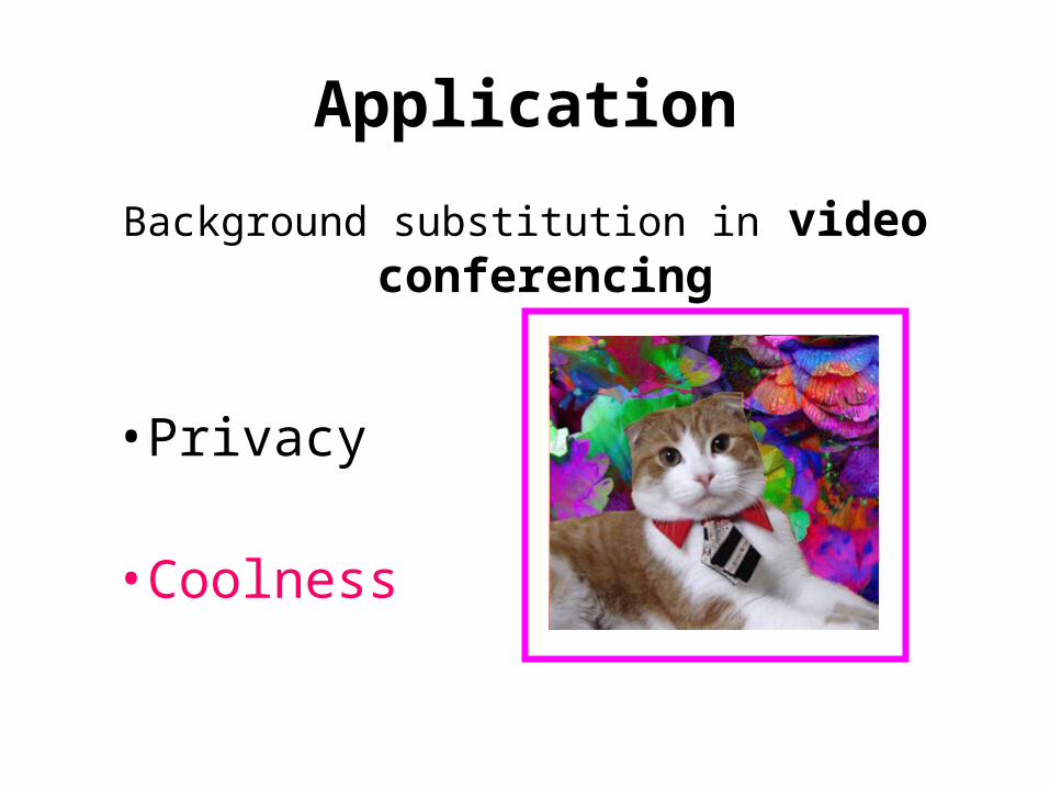
Modeling Contrast and Spatial Coherence
• Spatial coherence
• Contrast – inhibits the penalty
Csr
sr xx),(
),(22 pixels,
72 penalty
22 pixels, 21 penalty
)||||exp( 2*sr IIV
4
3
Segmentation mapsBlack: ForegroundWhite: Background

Algorithms Review
"Probabilistic fusion of stereo
with color and contrast for bi-layer segmentation", V. Kolmogorov
et al., CVPR 2005. Represents two stereo algorithms:
– LDP Layered Dynamic Programming
– LGC Layered Graph Cut
"Background Cut", J. Sun et
al., ECCV 2006, to appear
"Bilayer Segmentation of
Live Video", A. Criminisi et al., CVPR 2006, to appear
Stereo Bilayer Segmentation
Background Cut
Temporal Bilayer Segmentation

Stereo Bilayer Segmentation
Information:– Colour – Contrast
–StereoPrior:
– Spatial coherence
–Disparity coherence–Disparity-labeling relations
Stereo Bilayer Segmentation

Notations
F – foreground
B – background
O – Occluded
– disparity vector
BFxk ,
Stereo Bilayer Segmentation
OBFxk ,,
d

Stereo Bilayer Segmentation
• Want to find
)|(maxargˆ Ixxx
p
Stereo Bilayer Segmentation

Stereo Bilayer Segmentation
• Want to find
d
xxzdxIxx )|,(maxarg)|(maxargˆ pp
This is intractable!
Stereo Bilayer Segmentation

Dealing with Intractability
• LDP – Layered Dynamic Programming
– Defining a similar problem
– Separating to scanlines
– Solving with dynamic programming
)]]|,(max[maxargˆ zdxxdx
pd
xzdxx )|,(maxargˆ p
Stereo Bilayer Segmentation

Dealing with Intractability
• LGC – Layered Graph Cut
– Relaxing some dependencies on disparity
– Marginalizing over
– Solving with graph cut
d
Stereo Bilayer Segmentation

Energy Function
• Define a Gibbs energy
• Model it as
)|,(log),,( IdxxdI pE
CM UUVE ),,( xdI
Prior: Spatial Coherence + contrast
Likelihood: MatchingLikelihood: Colour
Stereo Bilayer Segmentation

The Prior V• Sum of binary and unary potentials:
• F:
– Spatial coherence
– Contrast dependency
k
kksrCsr
sr dxGIIVxxFV ),(),(),(),( *
),(
dx
CM UUVE ),,( xdI
Stereo Bilayer Segmentation

Recall:
• F:
– F,B,O
– Sophisticated switch
k
kksrCsr
sr dxGIIVxxFV ),(),(),(),( *
),(
dx
Csr
sr xx),(
),(
),(),( *
),(sr
Csrsr IIVxxF
Stereo Bilayer Segmentation
The Prior V
CM UUVE ),,( xdI

1* V
Recall:
• V*:
– e=0 same equation,
– e=1 dilution,
– e=0 no use of contrast,
k
kksrCsr
sr dxGIIVxxFV ),(),(),(),( *
),(
dx
1
)||||exp(),(
2* sr
sr
IIIIV
)||||exp( 2*sr IIV
01
10 * V15.0 * V
Stereo Bilayer Segmentation
The Prior V
CM UUVE ),,( xdI

• Sum of unary and binary potentials:
• G:
– Higher disparities in foreground
– Based on a threshold
– Uniform penalty
0dd
k
kksrCsr
sr dxGIIVxxFV ),(),(),(),,( *
),(
dxI
Stereo Bilayer Segmentation
The Prior V
CM UUVE ),,( xdI

Likelihood for Matching
• Distinguish Matched (F,B) from Occluded (O)
• Determine disparity
• Model as
• - balance between occlusion and bad matches
k
kkMk
M dxUU ),,(),,( IdxI
MkU
Stereo Bilayer Segmentation
CM UUVE ),,( xdI

Likelihood for Matching
N – measures quality of match between patches
– Classical SSD:
Additive + Multiplicative normalization Robustness
– NSSD:
Pk
PPPP RLRLS 2)(),(
22 ||||||||
||)()(||
2
1),(
PPPP
PPPPPP
RRLL
RRLLRLN
Stereo Bilayer Segmentation 10 N
CM UUVE ),,( xdI

Likelihood for Matching
Balance between occlusion and bad matches:
Preference for occlusion
Oxif
dxU
BFxifNN
k
kkMk
k
0
),,(
,)( 0
I
0NN
Stereo Bilayer Segmentation
CM UUVE ),,( xdI

Likelihood for Colour
• GMM’s for Foreground and Background– 20 mixture componenets
• Learn from previous frames
• Learn using EM– 10 iterations
)(
)(
kB
kF
Ip
Ip
Stereo Bilayer Segmentation
CM UUVE ),,( xdI

Likelihood for Colour
• Model as:• Too strong Balancing factor
k
kkCk
C xIUU ),(),( xI
OBxifIp
FxifIpxIU
kkB
kkF
kkCk
,)(log
)(log),(
2
10 t
00 t
)(
)(
kB
kF
Ip
Ip
Stereo Bilayer Segmentation
CM UUVE ),,( xdI

Fusion of Cues
Colour FusionStereo
Stereo Bilayer Segmentation
CM UUVE ),,( xdI

LDP Layered Dynamic Programming
Want: separation to scanlines
Recall:
• V – Sum on neighbouring pixels
• Use only horizontal cliques
Work on scanlines
CM UUVE ),,( xdI
Prior: Spatial Coherence + contrast
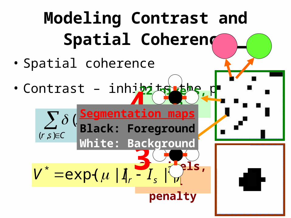
Stereo Bilayer Segmentation - LDP

LDP
• Classical DP
Diagonal: matched
Vertical: occluded
Horizontal: occluded
Stereo Bilayer Segmentation - LDP

LDP
• Layered DP
Alternates
between matched
and occluded!
Stereo Bilayer Segmentation - LDP

LDP
• Layered DP
The whole line
is matched!
Stereo Bilayer Segmentation - LDP

Stereo Bilayer Segmentation - LDP
LDP
• Layered DP
No diagonal moves
Vertical: matched or occluded
Horizontal: matched or occluded
LDP
• 4-State Space
• Many parameters:
• Learn parameters from labeled data
= mean width of matched region
= mean width of occluded region
00 ,,, bbaa
WOW
)log(: 21Wb
)log(: 21
OWOb
a – viewing geometry considerationsa0,c - normalization
Stereo Bilayer Segmentation - LDP
),(),( *
),(sr
Csrsr IIVxxF
W
1changefor yProbabilit

LDP
6-State Space
Stereo Bilayer Segmentation - LDP
CM UUGFVE *),,( xdI
Solve with dynamic programming!
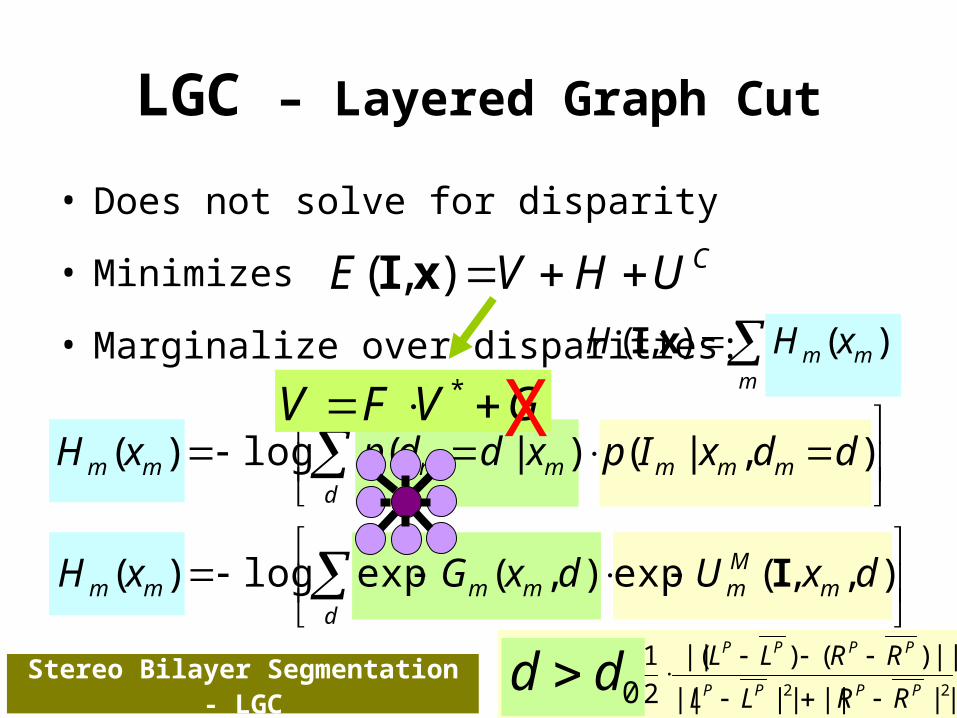
LGC – Layered Graph Cut
• Does not solve for disparity
• Minimizes
• Marginalize over disparities:
CUHVE ),( xI
dmmmmmmm ddxIpxddpxH ),|()|(log)(
m
mm xHH )(),( xI
dm
Mmmmmm dxUdxGxH ),,(exp),(explog)( I
Stereo Bilayer Segmentation - LGC 22 ||||||||
||)()(||
2
1),(
PPPP
PPPPPP
RRLL
RRLLRLN
0dd
GVFV * X

LGC• Expansion move algorithm
Stereo Bilayer Segmentation - LGC

LGC• Expansion move algorithm with savings:
– Only 3 Labels
– Only 2 iterations:
• Initialize with B for all pixels• Run F-expansion• Run O-expansion
OBF ,,
on a constrained region
Stereo Bilayer Segmentation - LGC

Results
LGCLDP
Stereo Bilayer Segmentation

Results (LGC)
Stereo Bilayer Segmentation

Results – Errors
Stereo Bilayer Segmentation

Quantitative Results
• Hand labeled ground truth (any 5th/10th frame)
• Percentage of misclassified
Stereo Bilayer Segmentation

Quantitative Results
• Hand labeled ground truth (any 5th/10th frame)
• Percentage of misclassified
Stereo Bilayer Segmentation

Quantitative Results
Stereo Bilayer Segmentation

Quantitative Results
Computation times:Around 10 fps at 320 X 240 resolution
On a conventional 3GHz processor
Stereo Bilayer Segmentation

Results
Stereo Bilayer Segmentation

Stereo Segmentation – Summary
• 2 algorithms: LGC and LDP
• Require binocular configuration
• Temporal relations are implicit
• Stereo cues are very strong
Stereo Bilayer Segmentation

Algorithms Review
"Probabilistic fusion of stereo
with color and contrast for bi-layer segmentation", V. Kolmogorov
et al., CVPR 2005. Represents two stereo algorithms:
– LDP Layered Dynamic Programming
– LGC Layered Graph Cut
"Background Cut", J. Sun et
al., ECCV 2006, to appear
"Bilayer Segmentation of
Live Video", A. Criminisi et al., CVPR 2006, to appear
Stereo Bilayer Segmentation
Background Cut
Temporal Bilayer Segmentation

Background Cut
Information:– Colour– Contrast
– Initialization phase
Prior:– Spatial coherence
Background Cut

- =
Most Efficient Approach:Background Subtraction
Background Cut

Problems:Foreground-Background similarity
Sensitive threshold
Most Efficient Approach:Background Subtraction
Background Cut

• Spatial coherence
• Colour model
Background maintenance
r
srNsr
r IIEIEIE ),()()(),(
21
(Minimize by min-cut)
Background Cut
Background Cut

Basic Model – Colour TermBackground: global and local
• Global: GMM model
)1510( bK
bK
k
bk
bkr
bkrr INBxIp
1
),|()|(
Background Cut

Background: global and local
• Global: GMM model
• Local: single Gaussian
Basic Model – Colour Term
)1510( bK
t
Background Cut

Background: global and local
• Global: GMM model
• Local: single gaussian
• Combination:
Basic Model – Colour Term
bK
k
bk
bkr
bkrrglobal INBxIp
1
),|()|(
),|()( Br
Brrrlocal INIp
)()1()|()( rlocalrrglobalrmix xpBxIpIp
Background Cut
)1510( bK

Foreground colour model
5 components GMM
Basic Model – Colour Term
frB tIp )(
Background Cut

Basic Model – Colour Term
BxifIp
FxifFxIpIxE
rrmix
rrrglobalrr
)(log
)|(log),(1
)()1()|()( rlocalrrglobalrmix xpBxIpIp
?Background Cut

)()1()|()( rlocalrrglobalrmix xpBxIpIp
Colour TermAdaptive mixture global-local colour model
Background Cut

Colour TermAdaptive mixture global-local colour model
How can we quantify the difference?
Kullback-Liebler divergence fbKL
Background Cut

Colour Term
Kullback-Liebler divergence
quantify the difference between two GMM’s
fbKL
)log)||((min0
bi
fkb
if
k
K
ki
fkfb w
wNNKLwKL
fbKL0sGMM'identical0 fbKL
Background Cut

)|()( BxIpIp rrglobalrmix 1fbKL
KL
fbKL
e 2
11
5.0
1fbKL
1
)()|()( 21
21
rlocalrrglobalrmix xpBxIpIp
Colour Term
Only Global
Equally Local and Global
Background Cut

Colour Term – Summary
)()1()|()()( rlocalrrglobalrmix xpBxIpIp
Background Cut
BxifIp
FxifFxIpIxE
rrmix
rrrglobalrr
)(log
)|(log),(
)(1

2
2
2
),(
|| sr II
Nsrsr exx
Basic Model – Contrast Term
Penalty term + Penalty inhibition
22sr II
2
, srsr IId
srd ,
Background Cut

Contrast Term
2
, srsr IId
Background contrast attenuation
Background Cut

Contrast TermForeground boundariesBackground contrast
Clues:
• Comparison to original background contrast
Background Cut

Contrast Term
Over attenuation of
boundaries!
2
2
,
1
1
K
IIsrsr
Bs
Br
IId
Background Cut
2
2
,
1
1
K
IIsrsr
Bs
Br
IId

Clues:
• Comparison to original background contrast
• Difference from original background
Contrast Term
Background Cut

Clues:
• Comparison to original background contrast
• Difference from original background
)exp(1
12,
2
2
,
z
srBs
Br z
K
IIsrsr IId
},max{,Bss
Brrsr IIIIz
Contrast Term
Background Cut

Contrast Term – Summary
+Background contrast+Background colour
+Background contrast
Background Cut

Contrast Term – Summary
Background Cut

Background Maintenance
Sudden illuminance change
• Auto gain control
• Fluorescent lamps
• Light switching
Background Cut

Background Maintenance
Minor change
• Histogram transformation function
Major change
• Colour model rebuilding
}{}{ BII rBr
Background Cut

Background MaintenanceColour model rebuilding
• Foreground threshold increasing
• Background uncertainty map initialization
• Mixture model modification
• Dynamic updating of and
1 Brur
)()1()|()( rlocalrrglobalrmix xpBxIpIp )()1)(1()|()( rlocalBrrrglobalrmix xpuBxIpIp
Bru B
rI
Background Cut

Background Maintenance
• Movement in the background
• Sleeping and waking objects
• Casual camera shaking
- Relying on global model
- Keeping biggest connected component
- Background maintenance- Appling Gaussian blurring
- Using less local colour model
Background Cut

Background Cut
Background Maintenance

Background Cut
Background Maintenance

Background Cut
Quantitative Results
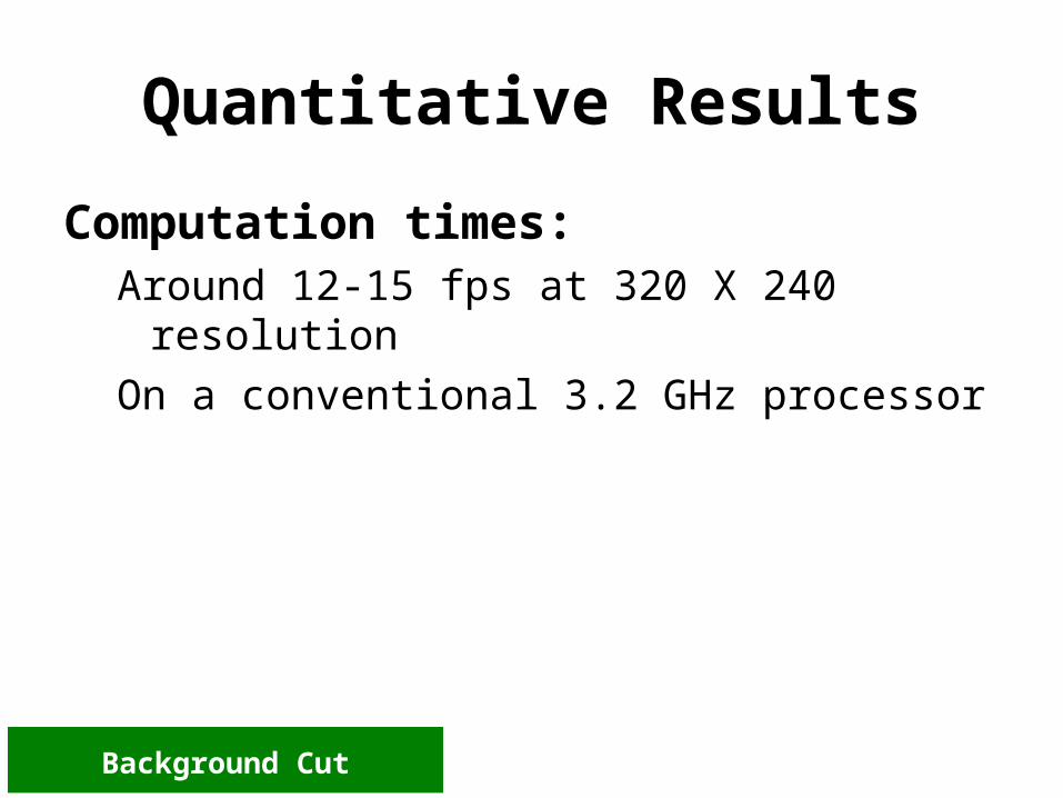
Quantitative Results
Computation times:Around 12-15 fps at 320 X 240 resolution
On a conventional 3.2 GHz processor
Background Cut

Background Cut – Summary• Adaptive mixture global-local colour model
• Background contrast attenuation
• Background Maintenance
Background Cut

Algorithms Review
"Probabilistic fusion of stereo
with color and contrast for bi-layer segmentation", V. Kolmogorov
et al., CVPR 2005. Represents two stereo algorithms:
– LDP Layered Dynamic Programming
– LGC Layered Graph Cut
"Background Cut", J. Sun et
al., ECCV 2006, to appear
"Bilayer Segmentation of
Live Video", A. Criminisi et al., CVPR 2006, to appear
Stereo Bilayer Segmentation
Background Cut
Temporal Bilayer Segmentation

Temporal Bilayer Segmentation
Information:– Colour – Contrast– Initialization phase
–MotionPrior:
– Spatial coherence
–Temporal coherence
Temporal Bilayer Segmentation

Motion – Notations
Basic image features (YUV)
),...,,( 21 NIII I )()( 1 tn
tnn IGIGI
),...,,( 21 Ngggg nn Ig )(grad
),( Igm
Temporal Bilayer Segmentation

Temporal Bilayer Segmentation
),,,,( 21 tttttt EE mIxxx
MCST UUVVE
• Temporal continuity• Spatial continuity• Colour likelihood• Motion likelihood
Temporal Bilayer Segmentation

Temporal Coherence4 pixel types:
Not likely: BFB, FBF
MCST UUVVE
Temporal Bilayer Segmentation

Temporal Coherence4 pixel types:
Not likely: BFB, FBF
MCST UUVVE
Temporal Bilayer Segmentation

Temporal Coherence4 pixel types:
N
n
tn
tn
tn
tttT xxxpV ),|(log),,( 2121 xxx
MCST UUVVE
Temporal Bilayer Segmentation

Spatial Coherence
The usual term:
MCST UUVVE
1
)||||exp()(),(
2
),(
nm
Cnmnm
S IIxxV Ix
Temporal Bilayer Segmentation

Likelihood for ColourGMM
– Number of mixture components– Learning:
• Initialization• Convergence• Time consuming
Histograms– Nonparametric– Smoothed to avoid overlearning
MCST UUVVE
XTemporal Bilayer Segmentation
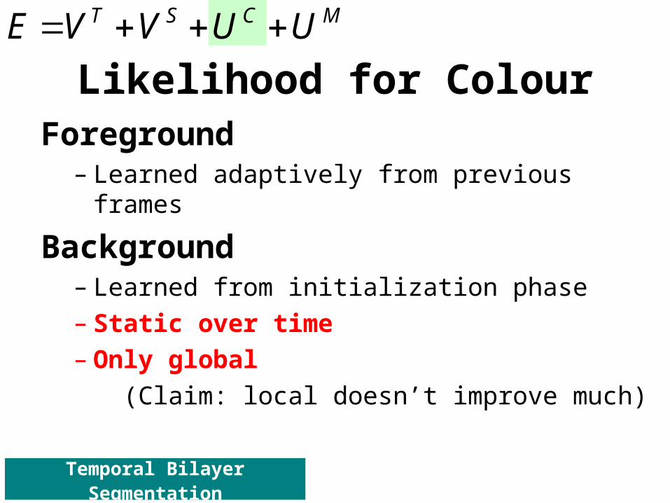
Likelihood for ColourForeground
– Learned adaptively from previous frames
Background– Learned from initialization phase– Static over time– Only global
(Claim: local doesn’t improve much)
MCST UUVVE
Temporal Bilayer Segmentation

Likelihood for Motion
Optical flow– Inaccuracies along boundaries
– The aperture problem
– Expensive
Motion/Non-motion classifier– Adaptive
– Efficient
X
MCST UUVVE
Temporal Bilayer Segmentation

Motion Classifier
Basic features:
MCST UUVVE
),( Igm
n
tn
tn
tn
tttM xxmpU ),|(log),,( 11 mxx ?),|( 1tn
tn
tn xxmp
Temporal Bilayer Segmentation

Temporal Bilayer Segmentation
Motion Classifier
MCST UUVVE
!X-axis:Grad(I)
Y-axis:I.
n
tn
tn
tn
tttM xxmpU ),|(log),,( 11 mxx
),( Igm

Testing the Motion Classifier
Not sufficient: Must fill in the gaps
Temporal Bilayer Segmentation

Minimizing the Energy
Want:
Instead:
),,,,( 21 tttttt EE mIxxx
t
t
tt Ep1'
'1 exp),...,( xx
t
t
tt E1'
'1 minarg),...,( xx
),,ˆ,,(minargˆ 21 tttttt Et
mIxxxxx
Allowing for changes in t-1
Temporal Bilayer Segmentation

Minimizing the Energy
Instead: ),,ˆ,,(minargˆ 21 tttttt E mIxxxxx
),,ˆ,,()ˆ|( 2111
1
tttttttt EpEt
mIxxxxxx
),,,,( 21 tttttt EE mIxxx
Temporal Bilayer Segmentation

Minimizing the Energy
Now minimize using Graph Cut
Instead: ),,ˆ,,(minargˆ 21 tttttt E mIxxxxx
),,ˆ,,()ˆ|( 2111
1
tttttttt EpEt
mIxxxxxx
Temporal Bilayer Segmentation

Results
Temporal Bilayer Segmentation

Quantitative Results
• Hand labeled ground truth (any 5th/10th frame)
• Percentage of misclassified
Temporal Bilayer Segmentation

Quantitative Results
• Hand labeled ground truth (any 5th/10th frame)
• Percentage of misclassified
Temporal Bilayer Segmentation

Limitations
High illuminance changes Failure (2/6 seq’s)
Recommend: switch off Auto Gain Control
Stereo V
Monocular X
Temporal Bilayer Segmentation

SummaryLDPLGCBackground
CutTemporal
Bilayer Seg.
Colour/ ContrastVVVVColour ModelGMM’sGMM’sGMM’sHistogramsBackground maintenanceVVV–DisparitiesExplicitImplicit––Background Attenuation––V–Motion–––VTemporal Coherence–––V

Another Approach to Background Substituition

Thank You!
A special thank to Dr. Vladimir Kolmogorov and to Eli Shechtman for their assitatnce
7.5.2006, Weizmann Institute of Science

F.A.Q.
Alon Rubin Shira Kritchman
7.5.2006, Weizmann Institute of Science

Likelihood for Matching
Empirical test – Is N discriminative?– Take labeled data– Compute and discretize N– Count matched pixels for each N– Count occluded pixels for each N– Divide
Get: Likelihood ratio of matching as a function of N
22 ||||||||
||)()(||
2
1),(
PPPP
PPPPPP
RRLL
RRLLRLN
CM UUVE ),,( xdz
Stereo Bilayer Segmentation

Likelihood for Matching
Example: Take N=0.1– 15% of matched pixels have N=0.1– 5% of occluded pixels have N=0.1
=> likelihood ratio for N=0.1
Get: Likelihood ratio of matching as a function of N
35
15
CM UUVE ),,( xdz
22 ||||||||
||)()(||
2
1),(
PPPP
PPPPPP
RRLL
RRLLRLN
Stereo Bilayer Segmentation

Likelihood for Matching
CM UUVE ),,( xdz
Stereo Bilayer Segmentation
Empirical results– X axis: Discretized values of N– Y axis: Log-likelihood ratio

Quantitative Results
• Hand labeled ground truth (any 5th/10th frame)
• Percentage of misclassified
Stereo Bilayer Segmentation

Stereo – Prior Parameters
LDP:
LGC:
Working parameters:
Baseline objects, todistance Nominal
)/11log()/1log(
BD
WBDa FF
)(2
1
)?F,( :Vertical
)BO,()OF,( :Horizontal
OF bb
F
BFF
mmBmmD
WWW FFO
50,1000
pixels 100 pixels, 10
Stereo Bilayer Segmentation

22 Bss
Brr IIII
Contrast Term
Background Cut
Alternative suggestion:
Inter-label attenuation

Dynamic updating of and
),|( 2,,, sr
Btrtr IIN
trB
trB
tr III ,,, )1(
)()()1( ,,,,2,
2,
Btrtr
TBtrtrtrtr IIII
))2/exp(1()1( 2,,,
trB
srtrBr
Br IIuu
Bru B
rI
Background Cut

Kullback-Liebler Divergence
)log)||((min0
bi
fkb
if
k
K
ki
fkfb w
wNNKLwKL
dxxq
xpxpQPKL
)(
)(log)()||(
Background Cut

VS Basic Model
Background Cut

Background Maintenance
Background Cut

Temporal Coherence Why 2nd order?
N
n
tn
tn
tn
tttT xxxpV ),|(log),,( 2121 xxx
MCST UUVVE
Temporal Bilayer Segmentation

Motion Classifier
MCST UUVVE
n
tn
tn
tn
tttM xxmpU ),|(log),,( 11 mxx
Why use spatial derivatives?
Temporal Bilayer Segmentation

Minimizing the Energy
Instead: ),,ˆ,,(minargˆ 21 tttttt E mIxxxxx
Z
xxxxp
xxpp
tttt
tt
n
tt
)ˆ,()1()ˆ|(
)ˆ|()ˆ|(
1111
1111
xx 1.0
),,ˆ,,()ˆ|( 2111
1
tttttttt EpEt
mIxxxxxx
Temporal Bilayer Segmentation

Results
Temporal Bilayer Segmentation

Results
With colour Without colour
Temporal Bilayer Segmentation