Embed Size (px)
Citation preview

Real-time Energy Consumption Feedback
Gonçalo Ramalho Freire de Andrade
Thesis to obtain the Master of Science Degree in
Electrical and Computer Engineering
Supervisors: Prof. Dr. Luís Miguel Veiga Vaz Caldas de Oliveira
Prof. Dr. Paulo Jorge Martins Parra
Examination Committee
Chairperson: Prof. Dr. António Manuel Raminhos Cordeiro Grilo
Supervisor: Prof. Dr. Luís Miguel Veiga Vaz Caldas de Oliveira
Members of the Committee: Prof. Dr. Carlos Augusto Santos Silva
November 2017

ii

iii
À memória do meu avô, Joaquim Ramalho.
O principal responsável pelo meu espírito
inovador e empreendedor, assim como, pelo
meu gosto por eletrónica e tecnologia.

iv

v
Acknowledgments
I would like to express my sincere gratitude to my mentor and thesis supervisor, Professor Doutor Luís
Caldas de Oliveira, for his patience, availability, encouragement and guidance. A humane person with
the brightest and innovative mind I have ever came across in my life; who has been teaching me that it
is not enough to think outside the box – thinking is passive – we must act outside the box.
I would like to show my gratitude to Professor Doutor Paulo Parra and João Rocha, from Faculdade de
Belas-Artes da Universidade de Lisboa, who were always there to help us in the design of our solution.
Also, I would like to express my gratitude to Diogo Henriques and Dário, from EnergyOfThings, for
providing the sensors as well as for their teachings on Internet of Things, electronics and PCB
manufacturing. I would also like to thank to all the participants who were involved in this work.
Finally, I must express my very profound gratitude to those who always believed in me, giving me
strength to achieve my goals and resources to conclude my education.
To my girlfriend Flávia, for her support and inexhaustible understanding. Without her, I would not be
able to fully concentrate in this work.
To my mother, who lifted me up whenever I fell, and who always believes in what she can’t yet see.
To my father, who always cared about my education, and who only believes in what he can really see.
To my grandmother Bea, who always supported my ideas, and who knows that “miracle” is another word
for “hard work”.
To my grandfather Joaquim, who was a creative entrepreneur, a long time ago.
To all other family members who believe in my dreams.
To all my friends who make my day, every day.
This accomplishment would not have been possible without everyone abovementioned. Thank you all.

vi
“The biggest risk is not taking any risk…
In a world that is changing really quickly,
the only strategy that is guaranteed to fail
is not taking risks.” – Mark Zuckerberg

vii
Abstract
Occupants’ behaviour plays a central role over a household’s energy consumption. However, electricity
is invisible for most consumers.
The goal of an Energy Feedback Device (EFD), also known as In-Home Display, is to make electricity
visible by presenting the real-time consumption information and consequently helping occupants to
control their energy usage. Nevertheless, most of these devices do not satisfy consumers’ preferences
over functionality and design. Thus, there is a need to make them user-friendly, as some householders
cannot understand the displayed information.
This thesis presents the design and test of a cloud-based EFD with differentiating features when
compared to those of most commercial products. The proposed EFD aimed to be informative, intuitive
and aesthetically pleasing. The goal was to bring energy savings by influencing residential consumers’
behaviour to be more energy efficient.
A quantitative analysis was conducted, whereby the treatment group’s participants reduced their
average energy consumption between 15% and 36%, when comparing the 30 days before and after the
installation of the EFD within their households. These results presented statistical significance when
using a paired t-test (95% of confidence level). In opposition, the control group, without the EFD,
increased its average consumption by 2% over a similar time frame.
A qualitative analysis was also conducted via survey to assess the participants’ opinions, showing that
the EFD fulfils the proposed requirements of being informative, intuitive and aesthetically pleasing.
Moreover, the participants claimed that all the other occupants interacted with the device and that the
EFD modified their consumption behaviour.
Keywords: Energy Consumption, Energy Feedback Device, Energy Savings, In-Home Display,
Residential Electricity Consumers

viii
Resumo
O comportamento dos residentes possui um impacto significativo no consumo de energia de uma casa,
porém, a eletricidade é invisível para a maioria dos consumidores residenciais.
O objetivo de um dispositivo de feedback de energia – Energy Feedback Device (EFD) ou In-Home
Display – é de apresentar a informação de consumo atual e consequentemente, ajudar os residentes a
controlar o seu uso. Todavia, o design e funcionalidades da maioria destes dispositivos não satisfazem
os seus utilizadores. Assim, é necessário melhorá-los, de forma a que todos os residentes
compreendam as informações apresentadas pelo dispositivo.
Esta dissertação apresenta o desenvolvimento e teste de um EFD com características diferenciadoras,
face às encontradas em produtos comerciais. O EFD pretende ser informativo, intuitivo e esteticamente
agradável. O seu objetivo é induzir a um comportamento de consumo eficiente e consequentemente,
proporcionar poupanças energéticas.
Através da análise quantitativa, verificamos que o grupo de tratamento reduziu o seu consumo entre
15% e 36%, aquando da comparação do consumo médio entre os 30 dias antes e após a instalação
do EFD nas suas casas. Estes resultados apresentam significância estatística aquando da aplicação
de um teste t (95% de nível de confiança). O grupo de controlo (sem o EFD) aumentou o seu consumo
médio em 2%.
Através de um questionário realizado aos participantes, chegamos à conclusão que o EFD cumpre os
requisitos propostos: informativo, intuitivo e esteticamente agradável. Além disso, os participantes
referiram que todos os ocupantes interagiram com o dispositivo e que este modificou o seu
comportamento de consumo.
Palavras-chave: Consumidores Residenciais, Consumo de Energia, Energy Feedback Device, In-
Home Display, Poupança de Energia

ix
Table of Contents
Chapter 1: Introduction ........................................................................................................................1
1.1 Background ...............................................................................................................................1
1.2 Research Question and Contributions .......................................................................................3
1.3 Thesis structure .........................................................................................................................5
Chapter 2: State of the art ...................................................................................................................6
2.1 Energy consumption and greenhouse gas emissions .................................................................6
2.2 Household’s energy consumption ..............................................................................................6
2.3 Electricity invisibility ...................................................................................................................7
2.4 Feedback of energy consumption and In-Home Displays ...........................................................8
2.5 Types of In-Home Displays ........................................................................................................9
Chapter 3: Competition and Customer Segments .............................................................................. 11
3.1 Competition Research and Analysis ........................................................................................ 11
3.1.1 Energy Monitoring and Feedback Systems’ Companies & Products .................................. 11
3.1.2 Energy Feedback Devices’ competitors ............................................................................ 14
3.2 Customer Segments ................................................................................................................ 15
3.2.1 Small and Medium Businesses ......................................................................................... 16
3.2.2 Hospitality Landlords ........................................................................................................ 16
3.2.3 Residential Consumers ..................................................................................................... 17
3.3 Conclusion .............................................................................................................................. 18
Chapter 4: Residential Energy Consumption Feedback Device Development .................................... 19
4.1 Goals of the Energy Feedback Device ..................................................................................... 19
4.2 Casing..................................................................................................................................... 20
4.2.1 Light study prototype ........................................................................................................ 20
4.2.2 PCB first mock-up – electronics and dimension ................................................................. 20
4.2.3 Casing design process ..................................................................................................... 21
4.3 Electronics & PCB Design (Hardware) ..................................................................................... 22
4.3.1 Microcontroller and Wi-Fi module (ESP-12F) .................................................................... 22
4.3.2 Base and Tower Light Circuits (WS2812B) ....................................................................... 23
4.3.3 Power Supply ................................................................................................................... 24
4.3.4 Logic Level Converter ....................................................................................................... 24

x
4.3.5 Printed Circuit Boards (PCBs) ........................................................................................... 24
4.4 Firmware ................................................................................................................................. 25
4.4.1 ESP8266 SDK and Firmware upload ................................................................................ 25
4.4.2 Feedback Device Firmware (Application Code) ................................................................. 25
4.4.3 Light Actuation Variables .................................................................................................. 26
4.4.3.1 Individual Light Actuation Variables ............................................................................ 26
4.4.3.2 Population Light Actuation Variables .......................................................................... 27
4.4.3.3 Aggregated Light Actuation Variables......................................................................... 27
4.4.4 Wi-Fi Network Configuration ............................................................................................. 28
4.5 Final Prototype ........................................................................................................................ 28
Chapter 5: Acquisition of Real Consumption Data ............................................................................. 30
5.1 Campaign................................................................................................................................ 30
5.1.1 Audience archetypes ........................................................................................................ 30
5.1.2 Campaign content ............................................................................................................ 30
5.1.3 Enrolment methods........................................................................................................... 31
5.1.4 Campaign methodology and Timeline of activities ............................................................. 31
5.1.5 Campaign Channels, Promotion and Results .................................................................... 32
5.1.5.1 Campaign I – Channel I: Energy and Environment Online Communities’ Article .......... 32
5.1.5.2 Campaign II – Channel II: E-mail to Engineering Students .......................................... 32
5.1.5.3 Campaign III – Channel III: Personal Contact ............................................................. 32
5.2 Selection of Participants and sensor’s installation .................................................................... 33
5.2.1 Selection Process ............................................................................................................. 33
5.2.2 Sensor configuration, installation and troubleshooting ....................................................... 33
5.3 Creation of a Database of Household Consumption Data ........................................................ 34
5.3.1 Household Characterization .............................................................................................. 34
5.3.2 Household Consumption Data Structure ........................................................................... 35
5.4 Conclusion .............................................................................................................................. 35
Chapter 6: Household Energy Consumption Forecasting Algorithm ................................................... 36
6.1 Goals, data and methodology .................................................................................................. 36
6.1.1 Databases ........................................................................................................................ 36
6.1.2 Training, Validation and Test Set ...................................................................................... 37

xi
6.1.3 Experimental system methodology.................................................................................... 37
6.2 Linear Prediction Forecasting Algorithm................................................................................... 38
6.2.1 Hypothesis I...................................................................................................................... 39
6.2.2 Hypothesis II..................................................................................................................... 39
6.2.3 Brief overview ................................................................................................................... 40
6.3 Decision Trees Forecasting Algorithm ..................................................................................... 41
6.3.1 Objectives, resources and evaluation ................................................................................ 41
6.3.2 Objective I: Number of days used for the training period ................................................... 42
6.3.3 Objective II: Forecasting method ....................................................................................... 43
6.3.4 Objective III: Pre-pruning parameters ................................................................................ 44
6.3.5 Objective IV: Number of input variables ............................................................................ 46
6.3.6 Objective IV: Final set of input variables ............................................................................ 47
6.4 Conclusion .............................................................................................................................. 48
Chapter 7: Implementation ................................................................................................................ 50
7.1 System Architecture ................................................................................................................ 50
7.2 Energy Data System ............................................................................................................... 51
7.2.1 Data Collection System..................................................................................................... 52
7.2.2 Data Manager System ...................................................................................................... 52
7.2.2.1 Master Gatherer ......................................................................................................... 52
7.2.2.2 Filter .......................................................................................................................... 53
7.2.3 Data Forecasting System .................................................................................................. 53
7.2.3.1 Extractor .................................................................................................................... 53
7.2.3.2 Forecaster ................................................................................................................. 55
7.2.3.3 Error Calculator.......................................................................................................... 55
7.3 Energy Feedback Web System ............................................................................................... 56
7.3.1 Feedback Device Web Service ......................................................................................... 56
7.3.2 Energy Feedback App ...................................................................................................... 57
7.3.2.1 Real-time Energy Feedback App ................................................................................ 57
7.3.2.2 Historical Energy Feedback App ................................................................................ 57
7.3.3 Web Panel ........................................................................................................................ 58
7.4 Conclusion .............................................................................................................................. 59

xii
Chapter 8: Experiment, Results and Evaluation ................................................................................. 60
8.1 Design of the Experiment ........................................................................................................ 60
8.2 Participants households’ characterization ................................................................................ 61
8.2.1 Characteristics of the participants’ household, building, occupancy and electricity supply
contract ..................................................................................................................................... 61
8.2.2 Appliances on the participants’ households ....................................................................... 62
8.3 Quantitative Results and Analysis ............................................................................................ 63
8.3.1 Comparison of the daily average of energy consumption between periods ........................ 64
8.3.2 Statistical test ................................................................................................................... 66
8.3.3 Mean percentage error ..................................................................................................... 67
8.4 Qualitative Results and Analysis .............................................................................................. 68
8.4.1 Placement, occupant’s engagement and motivation .......................................................... 68
8.4.2 Consumption feedback, aesthetics and impact on behaviour............................................. 69
8.4.3 Customer’s perspective .................................................................................................... 70
8.4.4 Web Panel and NFC Tag .................................................................................................. 70
8.5 Conclusion .............................................................................................................................. 71
Chapter 9: Conclusions and Future Work .......................................................................................... 73
9.1 Summary ................................................................................................................................ 73
9.2 Conclusions ............................................................................................................................ 74
9.3 Final overview ......................................................................................................................... 77
9.4 Future Work ............................................................................................................................ 78
References ....................................................................................................................................... 79
Annexes ........................................................................................................................................... 83
Annex 3: Annexes to Chapter 3 – Competition and Customer Segments ........................................... 83
Annex 4: Annexes to Chapter 4 – Residential Energy Consumption Feedback Device Development . 86
Annex 5: Annexes to Chapter 5 – Acquisition of Real Consumption Data .......................................... 88
Annex 6: Annexes to Chapter 6 – Household Energy Consumption Forecast Algorithm ..................... 90
Annex 8: Annexes to Chapter 8 – Experiment, Results and Evaluation .............................................. 94

xiii
List of Figures
Figure 1.1: Energy Puppet - “Normal Mode” (left), “Medium Mode” (centre) and “Too High Mode” (right)
(picture from [25])................................................................................................................................3
Figure 2.1: Factors affecting domestic energy use (picture adapted from [6]) .......................................6
Figure 2.2: Three types of display design – Numerical (left), Analogue (centre) and Ambient (right)
(picture from [6]) .................................................................................................................................9
Figure 3.1: Competitors’ Survey – Part II – Percentage of SwC vs. Sw-HwC with each feature .......... 13
Figure 3.2: The Energy Detective, Green Energy Options, Canary Instruments and Energy Orb (from
left to right) ........................................................................................................................................ 14
Figure 4.1: Casing Model I, energy consumption measures (Daily and Instant), placement of the PCB,
Tower and Base. ............................................................................................................................... 20
Figure 4.2: WS2812B LED, Ring of 24x WS2812B LEDs, Breadboard Prototype with ESP-12F and
placement of the components on Casing I ......................................................................................... 20
Figure 4.3: PCB layout (left), PCB top and bottom 3D-model (centre and right side) .......................... 21
Figure 4.4: Casing I (left), Casing II and its Base and Tower (centre), Casing III and its Base and Tower
(right) ................................................................................................................................................ 21
Figure 4.5: Final PCB’s circuits schematic ......................................................................................... 22
Figure 4.6: WS2812B LED, diagram and pins description (adapted from [28]) ................................... 23
Figure 4.7: Pre-final PCB (left) and Final PCB (right) ......................................................................... 24
Figure 4.8: Diagram of the Feedback Device’s Firmware operation (simplified) .................................. 25
Figure 4.9: Base and Tower LEDs’ population localization on the PCB (left) and on the casing (centre),
and light actuation variables’ hierarchy (right) .................................................................................... 26
Figure 4.10: Representation of the three available actions for the LEDs (Static, Blink and Fade In/Out)
and examples of colours employing RGB values ............................................................................... 27
Figure 4.11: Sequential and All Effect representation over time for a population of LEDs (Base or Tower)
......................................................................................................................................................... 27
Figure 4.12: Final Prototype of the Residential Energy Consumption Feedback Device – assembled
(left) and disassembled (centre) – and the diagram of the Instant Consumption Level and Daily
Consumption Percentage (right) ........................................................................................................ 28
Figure 4.13: Base of the device – Top (left) and Bottom (right) .......................................................... 28
Figure 5.1: Campaign methodology diagram for applicant’s acquisition ............................................. 31
Figure 5.2: Timeline of the campaign’s activities (2016) ..................................................................... 31
Figure 5.3: EnergyOT Optic Sensor (left) and Digital Energy Meter indicating the meter’s LED (right) 33

xiv
Figure 6.1: Simplified diagram of the experimental system methodology............................................ 37
Figure 7.1: Energy Feedback Device’s system architecture diagram.................................................. 50
Figure 7.2: Diagram of the Data Collection, Manager and Forecasting System (processes and
generated data files) ......................................................................................................................... 51
Figure 7.3: Web Panel Home Page for one of the participants ........................................................... 58
Figure 8.1: Normalized daily energy consumption average – comparing the 30-day before vs. after
period ............................................................................................................................................... 64
Figure 8.2: Energy savings of the treatment group (compared to the 30 days previous to the EFD
implementation) ................................................................................................................................ 65
Figure A.4.1: ESP-12F (left) and the schematic of its connections (right) ........................................... 86
Figure A.4.2: Final PCB and its connections to the 3.3V FTDI ........................................................... 86
Figure A.4.3: Screenshot of the Wi-Fi configuration methods: direct (left) and software configuration
(right) ................................................................................................................................................ 86
Figure A.5.1: Flyer (left) and Infographic (right) employed to disseminate information about the campaign
......................................................................................................................................................... 88
Figure A.5.2: Main Enrolment Method – Landing Page with Registration Form (www.energymonitor.xyz
– Accessed: 20/05/2016) .................................................................................................................. 88
Figure A.5.3: Promotion of the Campaign, through the Flyer, on DECO’s Portal for Renewable Energies
(http://energias-renovaveis-emcasa.pt – Accessed: 05/04/2016) ....................................................... 89

xv
List of Tables
Table 3.1: Competitors’ Assessment – Part I ..................................................................................... 11
Table 3.2: Competitors’ Assessment – Part II .................................................................................... 11
Table 3.3: Number of companies collected, selected and survey answers ......................................... 12
Table 3.4: Competitor’s Survey – Part I – Most common answers...................................................... 12
Table 3.6: Most common features of the Energy Feedback Devices (Hardware) ................................ 15
Table 3.7: Most common features of Sensor/Transmitter Units .......................................................... 15
Table 3.8: Hospitality Landlords’ interview - questions and answers .................................................. 16
Table 4.1: ESP-12F pins and respective connections ........................................................................ 22
Table 4.2: Light Circuits characteristics and additional components ................................................... 23
Table 4.3: Main modifications – Pre-final PCB vs. Final PCB ............................................................. 25
Table 4.4: Aggregated, Population and Individual light actuation variables ......................................... 26
Table 4.5: PCB, electronics and overall hardware price per hardware part ......................................... 29
Table 5.1: Characteristics of audience archetypes and desired mindset hypothesis ........................... 30
Table 5.2: Campaign content’s type, provided information and distribution format .............................. 31
Table 5.3: Enrolment methods provided to the audience, required fields and description ................... 31
Table 5.4: Installation Conditions’ parameters and description ........................................................... 33
Table 5.6: Characteristics of the household, occupancy and electricity supply contract ...................... 34
Table 5.7: Categories and appliances – multiple-choice survey ......................................................... 35
Table 6.1: Databases for the tests ..................................................................................................... 36
Table 6.2: Linear Prediction - Summary of Hypotheses I and II .......................................................... 38
Table 6.3: Linear Prediction – Hypothesis I – Mean Absolute Error results (in kWh) ........................... 39
Table 6.4: Linear Prediction – Hypothesis II – 9 experiments for the tests of ∆LPC vs. N ................... 39
Table 6.5: Linear Prediction – Hypothesis II – Mean Absolute Error results (K’=1) ............................. 39
Table 6.6: Equation 6.2 – Mean Absolute Error results (DB II Training Set) ....................................... 40
Table 6.7: Decision Trees – Objective I – Mean Absolute Error results (DB I) .................................... 42
Table 6.8: Decision Trees - Objective II – conditions of experiment 3 and 4 (DB II) ............................ 43
Table 6.9: Decision Trees – Objective III – Mean Absolute Error results of experiment 5 (DB II) ........ 44
Table 6.10: Decision Trees – Objective III – Mean absolute error results of experiment 6 (DB II) ....... 45
Table 6.11: Decision Trees – Objective IV – Mean absolute error results of experiment 7 (DB II) ....... 46

xvi
Table 6.12: Decision Trees – Objective IV – 11-variable ExtraTrees of experiment 7 vs. baseline mean
absolute error (DB II)......................................................................................................................... 46
Table 6.13: Decision Trees – Objective IV – Mean absolute error results of experiment 8 (DB III) ...... 47
Table 6.14: Decision Trees – Objective IV – Mean absolute error results of experiment 9 (DB IV)...... 47
Table 6.15: Characteristics of the Household Energy Consumption Forecasting Algorithm ................ 49
Table 7.1: System processes, data files and description .................................................................... 52
Table 7.2: Historical Data File – 14 Daily Variables............................................................................ 53
Table 7.3: 25 Variables common to the Training and Predictors Set .................................................. 54
Table 7.4: Instant Consumption Levels and limits representation ....................................................... 54
Table 7.5: JSON files, on Web Service, for the Real-time and Historical Energy Feedback App ........ 56
Table 7.6: Instant Consumption Levels – light actuation variables’ default values .............................. 57
Table 8.1: Participants’ answers on their household type, building, occupancy and electricity supply
contract ............................................................................................................................................. 61
Table 8.2: Electrical Appliances on each one of the participants’ household and overall results ......... 62
Table 8.3: Before and after energy consumption – daily average – in kWh and percentage .............. 65
Table 8.4: p-value results of the Paired T-Test ................................................................................. 66
Table 8.5: Mean Percentage Error results (before and after period) .................................................. 67
Table 8.6: Placement, location, occupant’s engagement and motivation answers .............................. 68
Table 8.7: Device ratings over aesthetics, real-time and daily consumption feedback and impact on
behaviour modification ...................................................................................................................... 69
Table A.3.1: Competitor companies’ exclusion factors ....................................................................... 83
Table A.3.2: Competitors’ survey – Part I – Results ........................................................................... 83
Table A.3.3: Competitors’ assessment – Part II – Percentage based on survey results ...................... 83
Table A.3.4: Competitors’ survey – Part II – Numerical results from answers ..................................... 84
Table A.3.5: Companies and products analysed on Energy Feedback Devices (Hardware)
categorization ................................................................................................................................... 84
Table A.3.6: Energy Feedback Devices (Hardware) features and results ........................................... 85
Table A.3.7: Electric Meter Sensor/Transmitter units features and results .......................................... 85
Table A.3.8: Landlords’ answers on energy consumption: appliances, energy efficiency measures and
type of electric meter ......................................................................................................................... 85
Table A.4.1: 2-Layer PCB Specifications ........................................................................................... 87
Table A.4.2: Box of Materials for each Final PCB and components’ prices, manufacturers and suppliers
......................................................................................................................................................... 87

xvii
Table A.5.1: Portuguese Energy and Environment Online Communities’ Information ......................... 89
Table A.5.2: Number of subjects for each campaign’s stage .............................................................. 89
Table A.6.1: Day’s assignment method for the Training, Validation and Test Set (e.g., first 10 days of a
year) ................................................................................................................................................. 90
Table A.6.2: Variables available for each day .................................................................................... 90
Table A.6.3: DB II and III – Number of total and valid days of each set .............................................. 90
Table A.6.4: Input variables available for each day (computed by the extractor and used by the
forecaster) ........................................................................................................................................ 90
Table A.6.5: Default values for the pre-pruning parameters of each forecasting function .................... 91
Table A.6.6: Definition of each pre-pruning parameter ....................................................................... 91
Table A.6.7: Decision Trees – Objective II – Experiment 3 – MAE results for the top 16 smallest values
(all associated to Extremely Randomized Trees) ............................................................................... 92
Table A.6.8: Decision Trees – Experiment 4 – MAE results (partial) – best overall results associated to
Extremely Randomized Trees and best MAE results from Regression Tree ....................................... 92
Table A.6.9: Decision Trees – Objective III – Experiment 5 – Type of input variables (chosen by the
greedy algorithm) .............................................................................................................................. 93
Table A.6.10: Objective III – Pre-pruning parameters tested and MAE results (kWh) ......................... 93
Table A.8.1: 30 days’ before vs. after period dates for each participant ............................................. 94
Table A.8.2: Energy values (kWh) ..................................................................................................... 94

xviii
List of Acronyms
API Application Programming Interface
CDD Cooling Degree Days
CSV Comma-separated values
DB Database
EFD Energy Feedback Device
EMF Energy Monitoring and Feedback
EMFS Energy Monitoring and Feedback System
HDD Heating Degree Days
HTTP Hypertext Transfer Protocol
IHD In-Home Display
JSON JavaScript Object Notation
LCD Liquid Crystal Display
MAE Mean Absolute Error
MPE Mean Percentage Error
NFC Near Field Communication
PaaS Platform as a Service
PHP Hypertext Preprocessor
kWh Kilowatt hour

Chapter 1: Introduction
1.1 Background
In Portugal, residential consumers are responsible for 26% of the final electricity consumption [1]. In
2014, Eurostat concluded that EU-28’s electricity, gas, steam and air conditioning supply activities by
households and industries had the largest share of greenhouse gas emission – whereby households
(19%) present the same amount of emissions as manufacturing (19%) [2]. These facts allow us to
understand the impact of households in both electricity consumption and greenhouse gas emissions.
Previous studies [4, 5, 7] identified the factors influencing household’s energy consumption – e.g.
building characteristics, environmental conditions, energy cost and appliances – however, these studies
placed the occupants’ behaviour as one of the main factors. A previous study [8] claimed the occupants’
behaviour is responsible for up to one third of the household’s energy consumption. However, this study
[8] was performed in the 80s; therefore, considering the increase of electricity consumption since then
to nowadays this result may be even higher. Another study [9] conducted for 10 identical homes with
similar equipment and appliances showed the influence of occupants’ behaviour: the most energy-
intensive house consumed 2.6 times more electricity than the least.
According to previous researches [10, 11] most of the residential consumers are unable to take steps
towards a more efficient use of energy. A considerable discrepancy exists between consumers’ self-
reported knowledge and their actual behaviour. A knowledge gap seems to be a potential constraint
among the consumers in identifying how their households consume energy [10]. Also, most consumers
show lack of attention towards energy prices and electricity suppliers’ market, which in turn prevents
them from adopting an electricity supply contract suitable to their needs [11].
The cost of a resource is usually related to its availability. Therefore, to use a resource efficiently, one
must have real-time information over its current price and/or amount spent so far vs. allocated budget.
In the case of electricity, this commodity is invisible to most of the residential consumers, as they only
know the cost of its usage after a long time. Thus, the monthly bill is not an appropriate tool for the
management of energy consumption, thereby making conservation practices for householders both
unusual and difficult [12]. This paradox was already identified in the 80s [13] using the following analogy:
“think of a store without a price tag on items, that presents the total single bill on the cash register”.
However, electricity suppliers still resort to a system with more than 40 years that is economically
unbeneficial for both parts; in addition to the negative effects on the environment due to the excessive
usage of energy.
Abrahamse [16] assessed 38 peer-reviewed studies on interventions to promote energy conservation
among households. These interventions were divided into two groups: antecedent interventions –
whereby providing previous information is assumed to influence the behaviour (e.g. commitment, goal
setting, information, and modelling); and consequent interventions – whereby the presence of a
positive/negative consequence is assumed to influence the behaviour (e.g. feedback and rewards). This

2
study concluded that “providing households with feedback, and especially frequent feedback, has
proven to be a successful intervention for reducing energy consumption”. Thus, a real-time feedback
system of the household’s energy consumption has the potential for larger energy savings.
To do so, we can resort to an Energy Monitoring and Feedback System (EMFS) – the so-called In-Home
Display (IHD) – by installing them on households to provide real-time energy consumption feedback.
According to several studies [19, 20, 21, 22] the IHD is the best way to both visualize and reduce a
household’s energy consumption. The use of these devices can bring energy savings from 4-15% [21]
or 5-15% [22].
In the literature, these systems are commonly referred to as In-Home Displays (IHD). In this work, we
will refer to them as Energy Monitoring and Feedback Systems (EMFS). In our perspective, the IHD
term from the literature is too closely linked to the feedback part of the system – commonly presenting
the consumption information through an LCD – as seen in [17]. The term Energy Monitoring and
Feedback Systems (EMFS), in our perspective, makes the concept clearer, as the system has a
monitoring part – which sends the real-time power data to the feedback device, usually through Radio
Frequency (the monitoring part can either be a smart meter, or a common electrical meter equipped
with a sensor and transmitter); and a feedback part – which displays the consumption information.
According to Darby’s categorization [23] there are three types of feedback displays design: numerical,
analogue and ambient. The numerical display presents the information through numbers (consumption
and/or its cost – through the associated units: currency, Watts and/or kWh) [6]. The analogue display
presents the information through graphs, charts and dials, instead of using numbers [6]. The ambient
display uses alternative ways to scales and numbers to present the consumption information, such as
light, movement or sounds [6].
We found several studies (e.g. [19, 20, 21]) analysing mainly numerical or analogue displays. Others
focus on the design issues of these types of display (e.g. [24]), as they are the most offered products in
the market. On the other hand, commercial products for energy feedback using ‘pure’ ambient displays
are almost inexistent. We only found Energy Orb [6], nevertheless, this device informs the user about
the current energy price, instead of informing about the household’s real-time energy consumption. Also,
studies focused on the design of ‘pure’ ambient displays (i.e. not mixing two types of display, e.g.
ambient and numerical) are almost inexistent. However, we found Energy Puppet [25] – “an ambient
device that provides peripherical awareness of energy consumption for individual home appliances,
producing different ‘pet-like’ behavioural reactions according to energy patterns”.
Figure 1.1 depicts the Energy Puppet in “Normal Mode” (green eyes and high arms), “Medium Mode”
(blue eyes with arms at medium height) and “Too High Mode” (red eyes, low arms and roar sound) [25].
Nevertheless, this was just a laboratory experiment, not being tested on real energy consumers and
only directed to individual appliances’ consumption feedback (instead feedbacking the household’s
energy consumption). Furthermore, in terms of aesthetics, we consider that improvements should be
done, previously to its test on real energy consumers. For those reasons, we consider there is a lack of
studies over designing ambient display, as well as testing them on households to provide energy

3
consumption feedback and ultimately lead to energy savings (through consumption behaviour
modification).
Figure 1.1: Energy Puppet - “Normal Mode” (left), “Medium Mode” (centre) and “Too High Mode” (right) (picture from [25])
Moreover, to back up the ambient displays’ potential over energy consumption feedback, we can resort
to Chiang [6] study. She tested, in a laboratory experiment, three types of ‘pure’ displays, and the
respondents preferred the numerical display (54%) over the ambient (34%) and analogue (32%) one.
However, another test was performed in this study. In a field experiment [6] where the investigator
placed the three types of ‘pure’ device on the dorm rooms of college students, the ambient display was
the one that brought much more positive results towards energy savings. This may lead us to perceive
a discrepancy over: what people think they want vs. what people really need.
Several studies shown the problems of current IHDs. The majority of UK’s IHD offered in the market do
not satisfy consumers preferences over functionality and design [24]. The IHDs are generally limited to
men and approaches must be taken to extend the scope of IHDs to women and children, by making
them more user-friendly, and consequently improving the effectiveness of these devices [20]. Many
householders are not willing to invest time to understand the usage of unintuitive IHDs [6]. The units
presented in the IHD are not understandable by some of the householders and there is a need to develop
unique feedback devices that user-friendly and provide accurate results [26].
1.2 Research Question and Contributions
The objective of this work is to find a process that brings energy savings by encouraging electricity
consumers to increase their energy efficiency. The proposed process will be implemented on
consumers’ households, to evaluate its effectiveness.
As presented in Section 1.1, the occupants’ behaviour plays a central role over the household’s energy
consumption. Moreover, previous studies showed that providing real-time energy consumption feedback
to the householders may change their behaviour towards an efficient one, and consequently bring
energy savings.
According to previous researches, the best way to visualize this information is through an Energy
Feedback Device (EFD) – the feedback component of an Energy Monitoring and Feedback System
(EMFS). In the literature, the EFD are commonly referred to as In-Home Displays (IHD) – usually
portraited as an LCD presenting the real-time energy consumption information.

4
Nevertheless, most of the offered EFD do not satisfy consumers’ preferences over functionality and
design. Furthermore, most of these devices present the units of consumption (e.g. Watts), which are
unperceivable by some of the householders (mainly, by women and children), preventing the adoption
of an efficient consumption behaviour from them, due to lack of understanding.
Therefore, we will develop our own Energy Monitoring and Feedback System, focusing on the Energy
Feedback Device’s design to address the existing problems (by using an ambient display, i.e., an
alternative way to the LCD with numbers and/or charts). The main research question is the following:
Can an Energy Feedback Device bring energy savings and be simultaneously pleasant and
informative to the consumer?
The main contribution of this work is to answer this research question. To do so, we had the need to
explore other related subjects. Therefore, the overall contributions of this work are the following:
• Assessment of the current Energy Monitoring and Feedback Systems’ market. We proposed a
framework to classify the existing products’ features and according to it, we surveyed 47
companies to obtain their products’ data. The objective was to find differentiating features for
our EMFS.
• Collection of potential customers’ opinions. We proposed three hypotheses for Energy
Feedback Devices’ customer segments, and performed interviews to identify their needs and
the most suitable customer segment for our product.
• Development of a new Residential Energy Consumption Feedback Device. We employed a new
approach for the design of this type of device, by considering the problems found in the
literature, the market analysis and the potential customers’ opinions.
• Acquisition and characterization of a small set of residential electricity consumers, as the
participants of our experiments. We developed a framework for their acquisition through a
campaign. Moreover, we proposed a framework for their household’s characterization, as well
as for the database of the participants’ energy consumption, that can be employed in future
works of this kind.
• Development of an algorithm to predict the following day’s energy consumption of a household.
We tested forecasting methods and their parameters, to create an algorithm that would predict
the following day’s energy consumption (used as a reference).
• Development of a framework for the overall system architecture, comprised by the cloud server,
software and hardware.
• Implementation and assessment of the Energy Feedback Device’s impact over the participants’
energy consumption. A quantitative analysis of their consumption before vs. after the
implementation of the device was performed. Moreover, a qualitative analysis was conducted
to evaluate the participants’ opinion over the device’s ability on providing consumption
information, its impact on modifying their consumption behaviour, as well as an assessment of
the device’s aesthetics.

5
1.3 Thesis structure
This thesis contains 9 main chapters, including this introductory one. The content is arranged as follows:
Chapter 2 reviews the existing literature on residential energy consumption. We explored the factors
influencing it, focusing on the impact of the occupants’ behaviour. The proposed solutions for influencing
the change of the householders’ behaviour into an efficient one and their problems are also presented.
Chapter 3 presents an analysis of the Energy Monitoring and Feedback Systems’ market, as well as
the interviews to potential customers. This chapter aims to identify the most suitable customer segment
for our product, as well as define differentiating features for our product, based on the analysis of the
competitors’ products features.
Chapter 4 shows the development of our Residential Energy Consumption Feedback Device, applying
the differentiating features discovered on the previous chapter. Moreover, in this chapter, we defined
the consumption information to be presented to the user, as well as the characteristics of the device,
namely, its casing, hardware and software.
Chapter 5 presents the campaign employed for the acquisition of residential energy consumers’
participants for our experiments. We presented a framework for the household’s characterization, as
well as for the database of the participants’ energy consumption.
Chapter 6 presents the process employed for the household energy consumption forecasting algorithm,
to find a forecasting method and its associated parameters to predict the following day’s energy
consumption of a household.
Chapter 7 depicts the framework employed for the overall system architecture, comprised by the cloud
server, hardware and software.
Chapter 8 shows the experiment results, assessing the impact of the proposed Energy Feedback
Device on the participants’ energy consumption.
Chapter 9 presents the conclusions of this work as well as suggestions for future work.

6
Chapter 2: State of the art
2.1 Energy consumption and greenhouse gas emissions
In Portugal, 26% of the final electricity consumption is from the residential sector [1]. In Europe,
households have a significant impact over energy consumption and greenhouse gas emissions.
According to Eurostat, in 2014, EU-28’s electricity, gas, steam and air conditioning supply activities, by
households and industries had the largest share of greenhouse gas emissions – whereby households
were responsible for 19% of the emissions and manufacturing for another 19% [2].
One of the most concerning issues is related to consumption of electricity and fuels by the households,
accounting for 25% of the total energy consumed [3]. Also, the consumers are interested in reducing
their electricity consumption to manage their budget and to sustain energy efficiency [3].
2.2 Household’s energy consumption
There are several factors influencing household’s energy consumption, however, the occupants’
behaviour plays a central role over this issue. Other factors, from the findings of the study conducted by
Chen [4] include the residential space, employment rates of the country (i.e., more employment leads
to more consumption) and environmental conditions. Besides the occupants’ behaviour, another study
[5] pointed out that socio-economic, demographic, electrical appliances, environment and building’s
structural characteristics also significantly affect the energy consumption of a household. Figure 2.1
presents the diagram adapted from Chiang [6], to illustrate Summerfield’s conclusions over the factors
affecting domestic energy use as well as their relationships [7].
Figure 2.1: Factors affecting domestic energy use (picture adapted from [6])
The diagram of Figure 2.1 shows the central role of the occupants’ behaviour over the remaining factors.
Moreover, occupants’ behaviour is the factor that can be more easily changed, when compared to the
building ones (as financial means are needed to increase building’s energy efficiency).
A previous research [8] estimated that up to one third of the household’s consumption is due to
occupants’ behaviour. However, this study was performed in the 80s. Nowadays, this value may even
be higher, when considering the increase of electricity consumption since the 80s.

7
Another study [9] was conducted for 10 identical electrical houses, with similar equipment and
appliances. The most energy-intensive house consumed 2.6 times more electricity than the least,
showing the occupant’s behaviour influence over energy consumption.
According to Frederiks [10] most consumers are unable to take the necessary steps for improving
energy conversion and efficiency. A considerable discrepancy exists between consumers’ values, self-
reported knowledge, intentions, attitudes and their actual behaviour. A knowledge gap seems to be a
potential constraint among the consumers in identifying how their households consume energy. The
researcher further highlighted that consumers do not qualify for rational decision-making in terms of
energy consumption as assumed by various economic models. Another research [11] highlighted the
consumers’ lack of attention towards energy prices, expectation related to switching cost and no
experience related to switching different energy suppliers demotivates them – impeding the adoption of
an electricity supply contract suitable to their needs.
2.3 Electricity invisibility
The cost a resource is usually related to its availability. Therefore, to use a resource efficiently, the user
must have information over its current price and/or amount spent so far vs. allocated budget. In the case
of electricity, this resource is invisible to most of the residential consumers, as they only know the cost
of its usage after a long time. As an example, in a car, the real-time consumption information is available.
The gas meter presents the amount of remaining fuel and the litres/100km measure presents the driver’s
real-time consumption behaviour. Car manufacturers offer this system as an integrated solution of their
energy-consuming product; while electricity suppliers do not offer any kind of system to their clients.
This is contradictory, as the reduction of residential energy consumption benefits economically both
consumer and supplier, in addition to its positive effects for the environment.
The use of a monthly bill is not a proper tool for the management of energy consumption, making
conservation practices for householders both unusual and difficult [12]. A study in the 80s [13] already
identified this paradox, using the following analogy: “think of a store without a price tag on items, that
presents the total single bill on the cash register” – however, electricity suppliers still resort to a system
with more than 40 years that is unbeneficial for both parts.
According to [14] the invisibility of energy is described as the lack of proper feedback to the consumer,
thereby making it impossible to control the household’s consumption.
Thus, it is not possible to measure the degree of energy consumption without feedback, ending up
leading to energy invisibility. It is crucial for the consumers to develop a certain understanding regarding
the consumption of energy, which would eventually lead to effective management. Some of the
household appliances consume much energy; due to lack of information people are not aware it, which
can significantly contribute to affect the electricity bill [15].

8
2.4 Feedback of energy consumption and In-Home Displays
Abrahamse [16] evaluated 38 peer-reviewed studies on interventions to promote energy conservation
among households, dividing them into two groups: antecedent and consequent interventions.
Antecedent interventions are aimed to influence underlying determinants, such as knowledge, that are
believed to influence behaviour (commitment, goal setting, information and modelling). Consequent
interventions assume that the presence of positive or negative consequences influence behaviour
(feedback and rewards). This study concluded that “providing households with feedback, and especially
frequent feedback, has proven to be a successful intervention for reducing energy consumption”. A real-
time feedback system of the household’s energy consumption has thus the potential for larger savings
in energy.
Considering the current state of technology, we can take advantage of Energy Monitoring and Feedback
Systems (EMFS), the In-Home Display (IHD) as presented in the literature – commonly, an LCD that
provides the real-time energy consumption of a household, by communicating with the household’s
electric meter [17]. However, in this work we will employ the term EMFS for the whole system and
Energy Feedback Device (EFD) for the so-called IHD. In our perspective, it makes the concept clearer,
as the system has a monitoring part – which sends the real-time power data to the feedback device,
usually, communicating though Radio Frequency (a smart meter, or a common electrical meter equipped
with a sensor and transmitter); as well as a feedback part – which displays the consumption information.
The IHD (or EFD) enables the consumer to determine how much energy is consumed and what is the
cost of consuming [18]. This device can be utilised to warn or alert the person to keep track of the energy
consumption.
Studies [19, 20, 21, 22] highlighted that IHDs are the key elements for visualizing and reducing the
energy usage. The units of IHDs commonly support USB connectivity, displays, screens and touch
buttons in order to provide interactive user interface. This device serves as a tool to monitor the
performance of energy usage and to reduce its consumption. The IHD device usually displays real-time
usage of electricity, weekly usage of energy, pricing alerts related to energy consumption. One of the
most significant aspects includes that one can compare the performance of newly installed appliances
with the previous ones, through the observation of the consumption difference. These devices shown a
reduction in household’s energy consumption from 4 to 15% through their usage [21].
According to [22], feedback can be viewed as a learning tool, enabling the energy consumers to learn
by experimentation. It can examine as a self-teaching technique. The feedback attempts to enhance the
efficiency of other information and highlights the control of energy consumption. The standard related
to the savings from a direct feedback includes the range of 5-15%. The significance of the meter includes
providing a point of reference for display and improved billing. The meter must be clearly visible in the
building.

9
2.5 Types of In-Home Displays
Based on Darby’s categorization [23] there are three types of display design – numerical, analogue and
ambient – according to how the consumption information is displayed. Figure 2.3 depicts each of them.
Figure 2.2: Three types of display design – Numerical (left), Analogue (centre) and Ambient (right) (picture from [6])
Numerical displays present the consumption information through numbers [6] (e.g. current power
consumption in Watts), thereby providing detailed quantitative information to consumers interested in
accurate and useful data [24]. This display type is the most common to date, but as displays become
more design-led it is likely to shrink in relative importance [24].
Analogue displays present the consumption information through scales (e.g. graphs, charts, dials,
etc.) rather than through numbers. These displays are easier to read and interpret when compared to
numerical displays, showing both quantitative and qualitative information [6,24].
Ambient displays do not use charts nor numbers, instead, the consumption information is presented
through other means, such as pictures, sounds, colours and/or lights [6]. These displays are aimed at
the peripherical vision, not requiring users’ detailed attention and providing the overall consumption
information [6,24].
Upon the literature review, we found that most studies address numerical and analogue displays, as
these are the most common display types on the market. On the other hand, commercial products
using a ‘pure’ ambient display (i.e. not mixing two display types, e.g., ambient and numerical) are
almost inexistent. Still, we found a reference to Energy Orb in [6], but this ambient display informs the
user about the current price of electricity, instead of showing the household’s energy consumption.
Thus, there is a lack of studies regarding the design and test of ambient displays. Yet, we found
Energy Puppet [25] (Figure 1.1) – “an ambient display device that provides peripherical awareness of
energy consumption for individual home appliances” producing different pet-like behavioural reactions
according to the appliances’ consumption patterns. However, this was just a laboratory experiment,
not being tested on real energy consumers nor directed to the household’s energy consumption
feedback. In terms of aesthetics, we consider that improvements should be done, before testing it on
real energy consumers.
However, Chiang’s study [6] backs up the ambient display’s potential over consumption feedback and
energy savings, when applied in the ‘real world’. In the laboratory experiment, the three ‘pure’ display
types were presented to the participants, whereby respondents preferred the numerical display (54%)
over the ambient (34%) and analogue (32%). In the field experiment, the three ‘pure’ display types

10
were installed in the dorm rooms of college students, concluding that (in the ‘real world’) the ambient
display performed better than the other two types, as regards to energy savings through the
modification of the consumption behaviour. Thus, we can grasp that there is a discrepancy between:
what consumers think they want vs. what consumers really need.
Furthermore, there are several problems with the currently available IHDs on the market. Many
householders are not willing to invest time to understand the usage of unintuitive IHDs [6]. According
to a study performed in the United Kingdom [24], consumers consider that most of the IHD offered in
the market do not satisfy their needs towards functionality, being also critical towards display design.
According to [20] the use of IHDs are generally limited to men. The researchers suggested that
approaches must be taken to extend the scope of IHDs to women and children in order to improve the
effectiveness of these devices. Certain amendments can be made in the devices to make them user-
friendly, which would eventually increase the knowledge of the consumers towards their energy
consumption. The findings of a previous study [26] highlighted that the units are not clearly
understandable by the users for most IHDs. Furthermore, there are other visualisation issues that
reduce the efficacy of IHDs in assessing the energy consumption. The researcher indicated that there
is a need to develop unique feedback devices that are user-friendly and provide accurate results.

11
Chapter 3: Competition and Customer Segments
In this chapter, we will research companies and products available on the market. The aim is to identify
the most suitable customer segment and innovative features for the development of our own system.
3.1 Competition Research and Analysis
3.1.1 Energy Monitoring and Feedback Systems’ Companies & Products
We conducted an exhaustive research of the existing Energy Monitoring and Feedback (EMF) systems,
from September 2015 to January 2016, with the objective of assessing the companies’ operating market
and identifying the features of their products.
In the first stage, we collected 162 companies with EMF products, providing either software and/or
hardware solutions.
In the second stage, we analysed the systems, creating 8 exclusion factors (Table A.3.1 on Annex 3) to
identify companies out of the scope of this work (e.g. “Solar Energy Companies”, which provide EMF
for generation, rather than for energy consumption). Based on these factors, we excluded 34 companies,
resulting in a final batch of 128 companies selected.
In the third stage, we created Table 3.1 and 3.2 with categories and features, to classify each
company and assess their EMF systems’ hardware and software features. These tables were
converted into a multiple-choice survey (available on http://bit.ly/2q9rJ2i) to be filled in by the
companies to obtain reliable and accurate insider information. We performed an extensive analysis of
the competitors’ systems’ most common features, summarized it on the least amount of categories
and features. Table 3.1 (Part I) categorizes the competitors into groups – operating market, system’s
hardware and data-related features – and Table 3.2 (Part II) presents the system’s software features.
Table 3.1: Competitors’ Assessment – Part I Competitors’ Assessment – Part I – Market, system’s hardware and data-related features
Category (Group) Definition
Market Company’s operating market(s) – Residential, Commercial and/or Industrial
Sensor Comp System’s compatibility with 3rd party electric meter sensors, or company-specific sensors
Add-on Hw Integration of additional hardware to the system – sub-metering, extra sensors and/or actuators (e.g. smart plugs)
En Dt Upd Rt System’s energy data update rate from the electric meter sensor (e.g. seconds, minutes)
Dt Access Type of access to collected/treated energy data – Web-based, Desktop and/or App
DB St Per System’s database storage period of energy data (e.g. months, years, lifetime)
Cons Units System’s units available to represent consumption – kWh, energy cost and/or CO2 emissions Legend: Comp – Compatibility; Hw – Hardware; En – Energy; Dt – Data; Upd – Update; Rt – Rate; DB – Database; St – Storage; Per – Period; Cons
– Consumption;
Table 3.2: Competitors’ Assessment – Part II Competitors’ Assessment – Part II – System’s software features on data analysis, treatment and presentation
Features Definition
Billing Energy Billing – Invoice’s import, storage (DB) and/or audit
Bench Energy Benchmarking – compare user’s past vs present energy consumption, or relate it to similar consumers
Forec Energy Forecasting – predict user’s energy consumption
Reports Energy Reports on benchmarking, billing, emissions or extra sensors’ data
DA&P Energy data analysis and identification of consumption patterns, providing useful insights to the user
UI User Interaction features – provide measures to reduce consumption, define alarms and allow user-input data Legend: DB – Database; Bench – Benchmarking; Forec – Forecasting; DA&P – Data Analysis & Patterns; UI – User Interaction

12
Finally, we requested the 128 companies, via e-mail, to fill in the survey. We contacted more companies,
via phone call, to convince them to fill in the survey as well as to collect additional information from the
potential client point of view. From this population, 47 companies answered the survey.
Table 3.3 illustrates each stage of the process (collection, selection and survey answers). The
companies were divided into 2 groups: SwC – companies providing software-only systems; and Sw-
HwC – companies providing software/hardware systems.
Table 3.3: Number of companies collected, selected and survey answers
Companies Group Group Description N. companies
collected N. companies selected
and contacted N. companies
answered survey
SwC Software-only 60 51 19
Sw-HwC Hardware and Software 102 77 28
Total 162 128 47 Legend: SwC – Software-only companies; Sw-HwC – Software and Hardware companies; N. - Number
Table A.3.2, on Annex 3, presents the 47 companies’ survey results for Part I. Table 3.4 compares the
most common answers given by software-only companies vs. software and hardware companies.
Table 3.4: Competitor’s Survey – Part I – Most common answers Part I – Survey Results from software-only (SwC) and software-hardware companies (Sw-HwC)
Company Type Market Sensor Comp.
Add-on Hw E. Acq.
Int. Data
Access DB St. Per.
Cons. Units
Most common SwC Industrial 3rd Party Sub
Metering
Minutes Web Based
Lifetime kWh Sw-HwC Commercial Specific Seconds
Legend: SwC – Software-Only Companies; Sw-HwC – Software and Hardware Companies; Comp. – Compatibility; Hw – Hardware; E. Acq. Int. –
Energy Acquisition Interval; DB St. Per. – Database Storage Period; Cons. – Consumption.
Most of the companies provide solutions for more than one market (most commonly, for both
Commercial and Industrial). Software-Hardware companies present more interest on the Residential
Market. Sub Metering is the most frequently supported hardware integration, while actuators are the
least supported. As to consumption units, next to kWh, the most common is currency/cost and the least
is CO2 level. Finally, software-hardware companies present a better energy data update rate (seconds
interval).
The most important findings are as follows:
• Industrial Market is not suitable for Energy Monitoring and Feedback Systems, as the market needs
specific energy monitoring needs depending on the sector of the Industry and the country’s energy
policy.
• Software solutions for EMF are the most common product on the market. To stand out from the
competition and innovate, we will focus on the development of a Hardware solution, although, we
will also have a software solution, available for the users, with the minimum requirements.
• Electric Meter’s Sensors are the second most marketable product. Due to the large number of
available sensors, we will not develop our own sensor Instead, we will take advantage of the web-
based access and use 3rd party sensors, as a source of energy data for our device.
• Sw-Hw companies’ hardware solutions are mostly comprised of company-specific sensors and
gateways as a means to provide data to company-specific or 3rd party software (local or Wi-Fi).
Also, most of these systems are only available for certain countries.

13
We found sensors working with 3rd party web platforms (software energy feedback), but we haven’t
found any Energy Feedback Device (hardware) compatible with 3rd party sensors.
Considering the findings, we decided to target the Residential/Commercial Market, by developing a
Hardware Energy Feedback Device, together with a cloud-based software solution that collects 3rd party
energy sensors’ data, controls the device and allows user access for further consumption data.
Table A.3.3 and A.3.4, on Annex 3, show the survey results for Part II. These features sought to
understand the competitor’s software abilities, namely, on converting raw energy data into useful
feedback information and insight to the user.
Figure 3.1 presents the percentage of companies possessing each one of the Part II features.
Figure 3.1: Competitors’ Survey – Part II – Percentage of SwC vs. Sw-HwC with each feature
Most of the software-only companies have all the previously presented features available on their
products, while most of the software-hardware companies do not have Billing features.
As to the Billing Features (i.e. importing, database and audit), the least common is “importing”. It may
be explained by the lack of availability of Web APIs from electricity supply companies to remotely access
consumption data from 3rd party software.
The third least common feature is Energy Forecast (prediction of future consumption), followed by
Benchmarking (relating user’s current vs past energy consumption).
Finally, Reporting, Data Analysis & Patterns and User Interaction are the most common features. The
most common feature on Reporting is the energy benchmarking report. On User Interaction, software-
hardware companies present Alarms as the most common, while software-only companies present Data
Input, as the most usual.
68%
89%
74%
100% 100%95%
43%
68%
57%
82% 82% 86%
0%
10%
20%
30%
40%
50%
60%
70%
80%
90%
100%
Billing Benchmarking Forecasting Reports Data Analysis &Patterns
User Interaction
SwC - Software-Only Companies Sw-HwC - Software and Hardware Companies

14
3.1.2 Energy Feedback Devices’ competitors
We decided to target the Residential and/or Commercial Market, developing a Hardware Device which
provides Real-Time Energy Feedback. In this section, we analysed the existing solutions, identifying
outdated product development patterns to be disrupted in order to bring innovation to these devices.
We’ve conducted an interview with Mark Mortimer, general manager of Wattsclever, pointing out that
the hardware energy monitors are better than software, as only “10% of the users recur to their App”.
Table 3.5 presents the categorization table created to analyze both Energy Monitoring and Feedback
System’s parameters, giving more emphasis to the Feedback Device analysis.
Table 3.5: Energy Feedback Devices Features (Hardware) System Features Value
Feedback Device
(feedback)
Information Presentation B&W LCD, Colour LCD, Light or LCD+Light
Display Design Numerical (numbers), Analogue (scales) or Ambient (other, e.g., light)
Power Plugged (electrical socket), Batteries or both available
Connectivity Radio-Frequency (RF) or Wi-Fi
Access Type to Data USB or Wi-Fi
Historic on Display If historical consumption data is shown on the Display
Forecast on Display If energy forecasting data is shown on the Display
Sensor & Transmitter (monitoring)
Type Current Transformer (CT), Optical Sensor or both available
Power Plugged (electrical socket), Batteries or both available
Connectivity Communication with the display – Radio Frequency (RF) or Wi-Fi
Minimum Update Interval Minimum available sensor’s interval to send data to the Display Legend: B&W – Black and White
As presented on Chapter 1, the energy displays can be classified into three categories: numerical –
information are presented through numbers; analogue – information are presented through graphs and
charts; or ambient – the information is illustrated by pictures, lights, colours or sounds. On January 2016,
we collected 20 energy feedback devices and 12 electric meter sensor/transmitter units from 12 different
companies, as presented on Table A.3.5, from Annex 3. Figure 3.2 illustrates several types of Energy
Feedback Devices (also known as In-Home Displays).
Figure 3.2: The Energy Detective, Green Energy Options, Canary Instruments and Energy Orb (from left to right)
The last two pictures present the Canary Instruments and Energy Orb, which are good examples of
ambient displays, where the consumption information is represented through light using the traffic lights
scheme. The Energy Orb is out of the scope, as it provides real-time feedback on energy prices’
changes, instead of presenting the household’s energy consumption feedback.

15
We categorized 20 Energy Feedback Devices (EFDs) based on the quantitative results available on
Table A.3.6, from Annex 3. The most common features are presented on Table 3.6.
Table 3.6: Most common features of the Energy Feedback Devices (Hardware) Presentation Design Powering Connectivity Data Access Historic Forecast
B&W LCD Numerical Plugged Radio Frequency USB Yes No
80% 50% 45% 95% 40% 85% 60% Legend: B&W LCD – Black and White Liquid Crystal Display.
Presentation of information and Display Design: Numerical displays using LCDs is the most common
type of display. Only the EFD from Canary Instruments used an ambient display design, by showing
colour-coded consumption information through light.
Connectivity: Radio-Frequency (i.e., other than Wi-Fi) is, by far, the most common type of
communication with the electric meter sensor.
Data Access: USB is the most common way to access data using desktop software.
Forecast: Most of the Feedback Devices do not present energy forecasting features.
We analysed the 12 Sensor/Transmitter Units associated to the 20 Energy Feedback Devices. The
results are presented in Table A.3.7 (Annex 3). Table 3.7 presents their most common features.
Table 3.7: Most common features of Sensor/Transmitter Units Sensor Type Powering Connectivity Minimum Update Interval
Current Transformer Batteries Radio Frequency <11 seconds
75% 67% 92% 58%
With regards to the Gateway responsible for sending the sensor’s monitoring data to the cloud, most of
the companies (50%) do not offer this equipment. From the ones who do, 40% offer it as optional
equipment; while 10% provide a required gateway with the system.
3.2 Customer Segments
We defined three hypotheses of customer segments for our Energy Feedback Device: Small and
Medium Businesses, Hospitality Landlords and Residential Consumers.
We interviewed subjects from each segment to validate if electricity costs are a “pain”. We then
assessed their opinions about the implementation of a real-time Energy Feedback Device to their
businesses or households, to reduce these costs and to obtain further electricity consumption
information. The interviews were conducted using certain guidelines. Although, we employed a strategy
of letting the respondent talk about other related issues to reach to new conclusions and to identify new
problems.

16
3.2.1 Small and Medium Businesses
We approached bars, pastries and/or restaurants, as they represent the most common Small-Medium
Businesses, with considerable electricity costs.
The owners claimed to pay an average of 1000-1200€ per month not performing any kind of analysis
with regards to the electricity bill. The general sentiment is that they cannot do anything about it. The
electric fryers and ovens are the appliances that consume the most electricity.
They do not have an interest in a real-time Energy Monitoring and Feedback System, claiming that they
cannot turn off an oven or a fryer if the Feedback Device tells them that they are using more energy
than necessary, as “the customer dictates the use of the appliances”.
The owners stated that the only option to reduce electricity costs was to apply energy efficiency
measures, such as: using LED lights, buying class A appliances, installing light sensors on the restroom,
educating employees by providing instructions to turn off lights and appliances when not needed,
avoiding stand-by consumption when closing the business and applying air conditioning measures
(turning off when not necessary and closing the windows and doors when using it).
To conclude, these businesses need long-term monitoring, to identify problems (appliances or
behaviours) and to apply better measures for energy efficiency that would lead to cost reduction.
3.2.2 Hospitality Landlords
Hospitality Landlords are homeowners who rent short-term lodging to tourists, using on-line hospitality
services’ platforms such as Airbnb. We resorted to this platform to obtain 23 Portuguese landlords
interested in providing a phone interview for this work. We formulated the hypothesis that energy usage
is their major operating cost due to the excessive consumption from tourists.
To solve this issue, we assessed their opinion on installing an Energy Monitoring and Feedback System
which would both provide remote information to the landlords and interaction with the tourists about their
real-time consumption through our hardware. Table 3.8 summarizes some of the most frequent
questions and their answers.
Table 3.8: Hospitality Landlords’ interview - questions and answers Landlords’ Answers
Yes Maybe No N.A.
Is electricity the major operating cost? 61% 22% 17% 0%
Do tourists have excessive energy consumption? 57% 17% 17% 9%
Is the landlord interested in monitoring remotely the energy consumption? 35% 30% 22% 13%
Is the landlord interested in installing an Energy Feedback Device to interact with the Tourists? 22% 35% 35% 9%
Is the landlord interested in actionable measures? * 39% 4% 9% 48%
Is the landlord interested in controlling the appliances remotely? 22% 17% 13% 48% *actionable measures are information from energy consumption data analysis to identify, for example, the most suitable electricity supply contract
Based on the landlords’ answers, we can conclude that electricity usage is their major operating cost,
mainly during winter, due to excessive consumption from tourists as they forget to turn off
heating/cooling appliances when leaving the house. After electricity, another cost is water usage, mainly
during summer. Some landlords have gas heating; therefore, electricity is not their major cost.

17
Some landlords (35%) were interested in monitoring the energy consumption remotely. Other 30% were
unsure about its usefulness, as they can watch, but not do anything about it. The ones with no interest
are usually older landlords with no interest in technology, or landlords with small houses and expenses.
As to the implementation of an Energy Feedback Device to interact with the Tourists, only 22% showed
interest, claiming that gamification should be applied (e.g. trying to beat last guests’ consumption) and
using the environmental cause as the main argument for saving. Most of landlords were either unsure
(35%), stating that it would work better on an ecological resort, or had no interest in the system (35%),
thinking that tourists will not interact with the device, or claiming that it is a “bad policy” to impose them
an energy efficient behaviour.
A good portion of the landlords (39%) were interested in actionable measures, to identify the “energy-
hungry” appliances and the most suitable electricity contract. Also, most of the asked landlords (22%),
presented interest in somehow controlling the appliances remotely, while others presented fears
regarding technology failures (older landlords) or turning off an appliance while it is in use by the tourist.
Table A.3.8, on Annex 3, presents the landlords’ answers towards their main sources of consumption –
oil-filled heater (38%) and air conditioning (22%); energy efficiency measures – LED lighting (58%) and
Class A appliances (25%); and type of electric meter – analog meter (52%) and digital meter (48%).
To conclude, landlords presented more interest in acquiring the system for their own home, where they
can actuate.
3.2.3 Residential Consumers
Some of the Small-Medium Businesses and Hospitality Landlords’ respondents were interested in
installing the system within their own houses, as they have more control over the energy consumption.
We interviewed 10 residential consumers to understand their interest and requirements for this kind of
solution. Eighty percent (80%) of the respondents confessed they feel they cannot control the energy
spent on their household, being open to the acquisition of a system that would help them save energy.
They proposed two methods for the acquisition: rented system – a monthly payment, smaller than the
saved energy value or buy system – buy the full system at an affordable price (around 120-150€) and
small fees for extra services, such as maintenance or installation of the system.
If the user is responsible for installing the system, respondents claimed that it must be “easy to install”,
as most of the respondents have some “fear” of touching their electrical panel.
Also, the energy consumption feedback, provided by the system, must be “easy to understand” and not
use very “technical details”, such as the units of consumption. Seventy percent (70%) prefer an always-
on hardware solution, instead of only having access to a software solution.
To conclude, considering their interest and the convergence of the other customer segments’ opinions
towards its use on their own house, we chose Residential Consumers as our target.

18
3.3 Conclusion
In our study of Energy Monitoring and Feedback Systems (EMFS) market, we found a lack of Energy
Feedback Devices (EFD) to provide hardware-based consumption information when compared with the
amount of software-based feedback solutions. Moreover, the electric meter’s sensor is the most
commonly offered hardware on this market. The companies usually focus on commercial and/or
industrial clients, disregarding the residential ones. In terms of customer segments, we’ve chosen the
Residential Consumers due to the interviews’ results.
We found that EFD on the market are mostly limited to receiving data from their own electric meter’s
sensor, not being compatible with third-party sensors. Therefore, the EMFS must be bought as a kit –
requiring a company-specific sensor with a coupled transmitter to communicate the real-time
consumption to the EFD, commonly, through Radio Frequency (i.e., not Wi-Fi). We found sensors
compatible with 3rd party software, but we haven’t found any EFD compatible with 3rd party sensors. We
also started to identify a trend in which the companies are starting to sell gateways, which allows the
sensor to send the household’s consumption data to the cloud.
Based on our study we decided to develop a Wi-Fi based Energy Feedback Device that can receive
consumption data from a variety of third-party electric meter’s sensors connected to the cloud. To
provide feedback of the consumption behaviour we will opt to use ambient display design by colour-
coding the measurements through light (instead of the commonly used LCDs) – to provide intuitive
consumption information to the users. Most of the manufacturers do not provide forecasting – we will
propose a solution for a forecasting algorithm to be used in our system. By taking advantage of the Wi-
Fi communication protocol, a web control panel will also be developed (i.e., software-based enegy
feedback). It would be accessible through browser and responsive (i.e., compatible with any device –
PC, smartphone and tablet), allowing access to further consumption data as well as to the configurate
of the Energy Feedback Device.

19
Chapter 4: Residential Energy Consumption
Feedback Device Development
In this chapter, we will start by defining the goals of the Energy Feedback Device (EFD) in terms of
electricity consumption presentation. Afterwards, we will delve into its casing, electronic components,
printed circuit board (PCB) and firmware.
4.1 Goals of the Energy Feedback Device
Our goal was to present the household’s electricity consumption to the users with the aid of light-
emission, on a USB-powered Wi-Fi EFD using the cloud to retrieve the electric meter’s sensor data. We
started by identifying two important electricity-related measures: Power (Watts) – unit of measurement
for the household’s current power consumption; and Energy (kWh) – the energy spent throughout the
current day. The energy is the integral of the power samples registered throughout a certain time
interval. To provide users with a greater capacity over their energy expenses, we defined this measure
as day-related. Therefore, our energy counter restarts at midnight.
Many manufacturers present the household’s power and energy values on their devices, thereby
requiring the user’s effort to understand the significance of the information. According to the interviewed
Residential Consumers (in Chapter 3) the information should be displayed in a user-friendly way.
Therefore, we proposed the reformulation of the power and energy presentation, by using levels and
percentages – which were colour-coded and presented to the user through light, as described below.
Instant Consumption Level (Power): the household’s real-time power consumption is presented in
levels. As a first approach, we started by using 6 levels: very low, low, medium, medium-high, high and
very high. We defined a light colour to each level based on the traffic lights scheme (i.e., low levels in
green, medium levels in orange and high levels in red). Moreover, we also defined light actions to
distinguish between levels with the same colour – whereby the first is a static light (no action) and the
second is a fade in/out light, e.g., the medium level is an orange static light while the medium-high level
is an orange light fading in/out. The householders’ objective is to maintain a low level as long as possible.
Daily Consumption Percentage (Energy): the household’s energy consumption up to the moment,
presented as a percentage of the predicted consumption for the day (by the Forecasting Algorithm –
see Chapter 6). We defined a light circle to represent the consumed (in orange) and remaining (in green)
daily energy percentage. The householder’s daily objective is to consume less than the predicted energy
for the day, i.e., to avoid the light circle to be fully orange.
To influence consumption behaviour, the device must be visible to all householders. For this reason, it
is highly desirable for the device to be as aesthetically pleasing as possible. To design the Feedback
Device, we benefited from the involvement of Professor Paulo Parra and his team, from FBAUL
(Faculdade de Belas Artes da Universidade de Lisboa), working together on the aesthetics, light study
and integration of the PCB.

20
4.2 Casing
The casing and PCB were developed side-by-side, therefore having a direct influence on each other’s
design. In this section, we will only present the most important breakthroughs. Considering the
objectives of the Feedback Device, FBAUL designed the first mock-up of the casing. Figure 4.1 presents
Casing I model (which was 3D-printed) for the first light study tests.
Figure 4.1: Casing Model I, energy consumption measures (Daily and Instant), placement of the PCB, Tower and Base.
The casing has a Tower, illuminated according to the Instant Consumption Level; and a Base,
illuminated according to the Daily Consumption Percentage. Due to the casing’s shape, a circular PCB
was designed to be placed between its Base and Tower.
4.2.1 Light study prototype
We started by using the 3D-printed model of Casing I, to check if the light feedback goals could be
fulfilled with its proposed shape. Figure 4.2 depicts the light study prototype electronics and Casing I.
Figure 4.2: WS2812B LED, Ring of 24x WS2812B LEDs, Breadboard Prototype with ESP-12F and placement of the components on Casing I
We built a breadboard prototype with the following components: WS2812B LED, to represent the Instant
Consumption Level; Ring of 24x WS2812B LEDs, to represent the Daily Consumption Percentage; and
ESP-12F, a Microcontroller and Wi-Fi module to actuate the LED and the Ring according to variables
retrieved from the cloud.
The light feedback goals were: the ring of LEDs would resemble a circular percentage scale (Daily
Consumption Goal) and the LED would provide information in levels through its light’s colour (Instant
Consumption Level). These goals were considered fulfilled for both the casing’s shape and electronic
components (Section 4.3 presents detailed information on the electronics).
4.2.2 PCB first mock-up – electronics and dimension
We designed the circular PCB’s first mock-up, to place all the electronics on a single board, and mainly
to serve as a guideline for FBAUL in terms of dimension for the design of the next versions of the casing.

21
Figure 4.3 depicts the layout and 3D-model of the PCB’s first mock-up.
Figure 4.3: PCB layout (left), PCB top and bottom 3D-model (centre and right side)
In terms of electronics, this PCB was the first draft. Later, some of the components remained (e.g.,
WS2812B LEDs) and others were replaced by more convenient ones (e.g., RGB LEDs, USB Type-A).
In terms of dimensions, this PCB had a 70.71 mm diameter along with 1.6 mm thickness. To screw the
PCB between the Casing’s Base and Tower, we created two holes with 2.5 mm of diameter inside a 52-
mm circumference. As a design requirement, its USB port must be accessible to the user.
4.2.3 Casing design process
FBAUL designed several casing versions, although, three of them were associated to the major
breakthroughs. Figure 4.4 presents Casing I, II and III.
Figure 4.4: Casing I (left), Casing II and its Base and Tower (centre), Casing III and its Base and Tower (right)
The shape of Casing I was validated for the previously defined light feedback goals. However, it had no
space for the placement of a PCB between its Base and Tower.
Casing II had a placement structure. A circular PCB could be screwed onto the Tower and the support
“legs” of the Tower could be placed onto the support holes of the Base. However, Casing II was not able
to clearly transmit the idea of a percentage scale, as its support “legs” break the smoothness of the
Base’s light for the Daily Consumption Percentage presentation. This problem led to the design of
Casing III – to keep the shape of Casing I and to place the support “legs” in a way that would not interfere
with the Base’s light.
Casing III combined the desired shape with a suitable placement structure: three “legs” within the interior
of the Tower and three holes within the interior of the Base, circumscribed on a 52-mm circumference.
The PCB was placed between the Base and the Tower, with the Tower’s “legs” screwed onto the Base’s
holes. The Final Casing (see Section 4.5) was based on minor improvements of Casing III.

22
4.3 Electronics & PCB Design (Hardware)
In this section, we will present the electronic circuits and components for the PCB of the Final Prototype.
Figure 4.5 depicts the circuits’ schematics, divided in four groups.
Figure 4.5: Final PCB’s circuits schematic
Microcontroller and Wi-Fi Module (ESP-12F): The main part of the system, responsible for the Wi-Fi
connection and for the control of the circuits through its GPIOs – powered with 3.3V.
Base and Tower Light Circuits (WS2812B): Responsible for providing the light feedback to the user,
using two groups of LEDs connected in series – powered with 5V.
Power Supply: The PCB had two voltages – 5V and 3.3V (on V_BATT and +3V3, Figure 4.5). The
Micro USB Input supplies the 5V and the Low-Dropout Voltage Regulator converts the 5V into 3.3V.
Base and Tower Logic Level Converter Circuits: Each Light Circuit had its own Logic Level Converter
circuit – stepping up the ESP-12F’s 3.3V commands to 5V commands – to receive the right logic level
signal (high or low).
4.3.1 Microcontroller and Wi-Fi module (ESP-12F)
The ESP8266 is a low-cost Wi-Fi chip with complete TCP/IP protocol stack and ultra-low 32-bit
microcontroller unit. We used the ESP-12F module, with 16 GPIOs and 4 MiB of built-in flash [27]. Figure
A.4.1, in Annex 4, depicts the ESP-12F and its circuit schematic. Table 4.1 presents its connections.
Table 4.1: ESP-12F pins and respective connections PIN Connection PIN Connection
REST Connected to GPIO16 TXD (*) Connected to pin header for transmitting data
ADC Unused RXD (*) Connected to pin header to receive data
CH_PD Powered with 3.3V (pull-up resistor)
GPIO4 Connected to the Tower’s Light Circuit through its Logic Level Converter
GPIO16 Connected to REST GPIO5 Connected to the Base’s Light Circuit through its Logic Level Converter
GPIO14 (*) Unused GPIO0 (*) Powered with 3.3V through pull-up resistor
GPIO12 (*) Unused GPIO2 (*) Powered with 3.3V through pull-up resistor
GPIO13 Connected to the Switch Circuit GPIO15 Connected to ground
VCC (*) Powered with 3.3V GND (*) Connected to ground (*) PINs available for external connections, through the associated PIN Header, for several purposes, such as programming

23
The 10 kΩ resistors are pull-up resistors, connected between their respective GPIO and 3.3V power
source, to ensure the signal is at a valid logic level if a high-impedance is introduced.
GPIO4, GPIO5 and GPIO13 are the main pins of the PCB, controlling the Tower’s Light Circuit, Base’s
Light Circuit and Switch Circuit, respectively.
The Switch Circuit on GPIO13 triggered the Wi-Fi Configuration Mode (Section 4.4.4), to configure the
network to which the ESP-12F is connected to. Its two parallel capacitors of 10µF and 0.1 µF let high
frequency noise through ground, so it does not disrupt the circuit.
GPIO16 is connected to REST, allowing the use of deep sleep functions. Although, due to our objective
of being an always-on real-time feedback device, this function was not used.
4.3.2 Base and Tower Light Circuits (WS2812B)
The Light Circuits used the WS2812B LED, from Worldsemi, an intelligent control LED light source that
the control circuit and RGB chip are integrated in a package of 5050 components [28]. Figure 4.6
presents the WS2812B, the diagram of its 4 pins and their description.
Figure 4.6: WS2812B LED, diagram and pins description (adapted from [28])
The common RGB LED uses 3 inputs to define the colour of a single LED. In opposition, WS2812B only
needs 1 input to define the different colours for a group of LEDs connected in series.
The LED’s accepted power supply voltage varies between 3.5 to 5.3V and each LED consumes an
average of 20 mA. We supplied 5V, as it provides a higher luminous intensity compared to a power
supply of 3.3V. Also, the USB transformers have an output of 5V, allowing the direct power supply.
We developed two Light Circuits with LEDs connected in series and arranged as a circumference on
the PCB. Table 4.2 presents the characteristics of these circuits and their additional components
Table 4.2: Light Circuits characteristics and additional components
Light Circuit Number of LEDs Placement on PCB Circumference radius ESP-12F
GPIO In-line resistors Capacitors
Base 22 Top 32 mm GPIO5 (*) 1x 470 Ω 21x 0.1 µF
Tower 6 Bottom 8 mm GPIO4 (*) 1x 470 Ω 5x 0.1 µF (*) Before reaching to the Light Circuit passes through the circuit’s Logic Level Converter (from GPIO5_LV to GPIO5_HV and GP IO4_LV to
GPIO4_HV – for the Base and Tower Light Circuit, respectively)
We used an in-line resistor of 470 Ω, placed on the DIN of each Light Circuit’s first LED, to avoid voltage
spikes and to limit the current into the input pin. We used a 0.1 µF capacitor, on the LED’s power supply
terminals, to smooth out the power supply. We chose a KEMET Multilayer Ceramic Capacitor, as it
bears proper characteristics to be used with LEDs, namely, due to these capacitors’ heat resistance.

24
4.3.3 Power Supply
The PCB is supplied with 5V through its micro USB input. The Low-Voltage Dropout (LDO) converts the
5V into 3.3V. Due to the casing design, we used a USB input mounted vertically onto the PCB (Micro
USB B Input Vertical).
The 5V are mainly used to power the Light Circuits and the 3.3V are mainly used to power the ESP-
12F. We placed a 10µF capacitor on the voltage regulator’s input and a 22µF capacitor on its output.
These are two basic bypass capacitors, used for filtering and stability, to soak up changes in
instantaneous load. As this is a linear voltage regulator (opposite to switching ones), filtering is not going
to be critical, although, we’ve used them as a precaution, mainly for stability. The 10µF to 22µF ratio is
fairly common for such voltage bypass.
4.3.4 Logic Level Converter
The WS2812B LED data input (DIN) signal’s logic levels are defined by the following voltages:
VIH=0.7VDD (High) and VIL=0.3VDD (Low). The ESP-12F is powered with 3.3V and WS2812B with 5V
(VDD), therefore we need a logic level converter to avoid misinterpretation of the signal’s logic level sent
by the ESP-12F. The presented circuit (Figure 4.5) is a Bi-Directional MOSFET Voltage Level Converter
(3.3V to 5V). Each circuit is constituted by the MOSFET Transistor BSS138 (N-Channel Logic Level
Enhancement Mode Field Effect Transistor) as well as by 2 pull-up resistors of 10 kΩ.
When the Low voltage side transmits a ‘1’ (3.3V), the MOSFET is tied high (off) and the high voltage
side “sees” 5V through its 10 kΩ pull-up resistor. When the low voltage side transmits a ‘0’ (0V), the
MOSFET source pin is grounded and the MOSFET is switched on, pulling down the high voltage side
to 0V. This way we guarantee that each group of WS2812B LEDs distinguishes the HIGH from the LOW
sent by the ESP-12F, not being influenced by the voltage variations around the 5V coming from the USB
transformer.
4.3.5 Printed Circuit Boards (PCBs)
The previously presented circuits are related to the Final PCB version. We developed a Pre-final PCB
version, to be tested and to find improvements for the final one. Figure 4.7 presents both versions.
Figure 4.7: Pre-final PCB (left) and Final PCB (right)
Some modifications were made from the Pre-final PCB to the Final PCB. They are as follows: increase
of Tower’s light intensity; improvement of the support holes; and implementation of the Logic Level

25
Converter circuits to deal with transformers’ supply voltage changes. Table 4.3 presents these
modifications in detail.
Table 4.3: Main modifications – Pre-final PCB vs. Final PCB Pre-final PCB Final PCB
Tower’s Light Circuit 4 LEDs arranged on a square 6 LEDs circumscribed on a 17-mm circumference
Support holes 6 holes with 2.8 mm, arranged on each 45 of a 51-mm circumference
3 holes with 3.5 mm, as vertexes of an equilateral triangle circumscribed on a 49-mm circumference
Circuits - Implementation of a Logic Level Converter Circuit associated with each Light Circuit
The full description of the electronics employed on the Final PCB are available on Section 4.5 (Final
Prototype).
4.4 Firmware
4.4.1 ESP8266 SDK and Firmware upload
The ESP8266 has an official Software Development Kit (SDK), allowing the chip to be directly
programmed [27]. However, there are several open source unofficial SDKs, such as NodeMCU and
Arduino – which are Lua-based and C++ based firmware, respectively.
We tested both, ending up choosing Arduino, due to its larger number of both documentation and
libraries, enabling the chip to be programmed like any other Arduino Device through Arduino IDE. To
upload the firmware to the PCB, we used a 3.3V FTDI, as the ESP-12F is powered with 3.3V and its TX
and RX signals to transmit and receive packets have the same voltage. The FTDI FT232RL converts
RS-232 or TTL serial transmissions to USB signals [29]. Figure A.4.2 (Annex 4) illustrates the
connections between PCB and 3.3V FTDI.
4.4.2 Feedback Device Firmware (Application Code)
The Feedback Device was only responsible for interpreting the light variables to perform the light
actuation for both its Base and Tower. The energy-related computation to transform the energy data
into light actuation variables was carried out in the cloud server (see Chapter 7). Figure 4.8 presents a
simplified diagram of the Feedback Device’s firmware, in terms of acquisition, parsing, interpretation
and actuation of the light variables.
Figure 4.8: Diagram of the Feedback Device’s Firmware operation (simplified)

26
The Energy Feedback Device starts by requesting the Feedback Device Data File (fbdata.json) to the
Web Service using a hard-coded unique identifier of 8 digits (deviceID) to identify itself. The Web Service
returns the Feedback Device Data file, containing all the light actuation variables for the Feedback
Device’s light actuation. The request rate is 6 seconds. If the light actuation duration is larger than 6
seconds, the device will wait until it finishes, otherwise, if it is less than 6 seconds, the device will repeat
the action. If the action ended and 6 seconds have passed, a new request is made.
4.4.3 Light Actuation Variables
The light actuation variables’ structure was designed analogously to a human cell population. Each cell
has individual “variables”, which are activated upon an external stimulus. This external stimulus dictates
the way these “variables” are activated individually to perform a population action.
We defined three groups of Light Actuation Variables: Individual – defines each LED’s colour and
action; Population – defines the population (Base and Tower) effect and LED’s action period; and
Aggregated – defines the order of the Base and Tower Population variables’ actuation. Table 4.4
presents an overview of the Individual, Population and Aggregated light actuation variables, contained
on the Feedback Device Data (fbdata.json) and interpreted by the Feedback Device.
Table 4.4: Aggregated, Population and Individual light actuation variables Variable Target Inputs Value
Aggregated Base & Tower Order ‘0’ – Simultaneous ‘1’ – Base, Tower ‘2’ – Tower, Base
Population
Base
Effect ‘0’ – All ‘1’ - Seq
Action duration Duration of the Base’s LEDs action, in ms.
Pause duration Interval between adjacent LEDs actuation if Effect = ‘1’
Tower
Effect ‘0’ – All ‘1’ - Seq
Action duration Duration of the Tower’s LEDs action, in ms.
Pause duration Interval between adjacent LEDs actuation if Effect = ‘1’
Individual Base (22) LEDs action, red, green, blue
Tower (6) LEDs action, red, green, blue Legend: ms – milliseconds; Seq - Sequential
Figure 4.9 presents the Base and Tower LEDs’ Population on the PCB and on the casing, as well as
the hierarchy the three variables’ type.
Figure 4.9: Base and Tower LEDs’ population localization on the PCB (left) and on the casing (centre), and light actuation variables’ hierarchy (right)
4.4.3.1 Individual Light Actuation Variables
Each LED has an individual action and colour. The colour uses the RGB colour model, through the
variables red, green and blue – with values between 0 and 255. The LED’s action may be Static, Blink,
or Fade In/Out, defined by the value of 0, 1 or 2, respectively. The period of each action depends on the
Population Light Actuation Variables associated to the LED.

27
Figure 4.10 depicts the three actions available for each LED and exemplifies RGB values for some
colour
Figure 4.10: Representation of the three available actions for the LEDs (Static, Blink and Fade In/Out) and examples of colours employing RGB values
On the Static action, the LED adopts its light colour instantaneously and stays with it. On the Blink, the
LED adopts its colour instantaneously, over a small period of time, and then turns it off. On the Fade
In/Out, the LED adopts its colour gradually (Fade In) and turns itself off, gradually (Fade Out). Each LED
of a population has its own colour and action assigned; although, the action’s period is defined by its
associated Population Light Actuation variable called action duration.
4.4.3.2 Population Light Actuation Variables
We have two populations of LEDs: Base and Tower. We defined two effects for the population:
Sequential – the action and colour defined for each LED are executed sequentially (the next LED will
only be actuated after the end of the previous LED’s action); or All – the LEDs of the population execute
their individual action all at the same time. Figure 4.11 exemplifies each effect for a population.
Figure 4.11: Sequential and All Effect representation over time for a population of LEDs (Base or Tower)
We also defined two possible interns of time associated to the effects: Action duration – interval of
time, in milliseconds, for each LED’s action period; Pause duration – interval of wait, in milliseconds,
between adjacent LEDs’ actions, being only used on the Sequential Effect.
4.4.3.3 Aggregated Light Actuation Variables
The Aggregated Variables are responsible for dictating the order of the Population Variables actuation
(Base and Tower) using the variable Order.
If Order = 0, the effects defined for the Base and Tower will be performed at the same time. If Order =
1, the Base will be actuated first followed by the Tower. If Order = 2, the Tower will be actuated first
followed by the Base.

28
4.4.4 Wi-Fi Network Configuration
Upon the Feedback Device’s start up, if it cannot connect to any Wi-Fi network, it’s Base and Tower will
glow red. On the bottom of the Feedback Device’s Base, there is a Button. To proceed to the
configuration of a Wi-Fi Network, the user must press the button with the device turned off and keep it
pressed while connecting the USB cable to the USB input, i.e., when powering up the device. The device
will glow blue, while in the Wi-Fi configuration mode, opening a Wi-Fi Network called BeAwareConfig.
The user must connect to this network and then configure the device for the desired network through
one of two ways: Direct configuration – by using the browser to access http://192.168.4.1 and inserting
the credentials of the desired network (SSID and Password); or Software configuration – we created
a Java executable, using a form to fill in the desired Wi-Fi network’s credentials. After the configuration,
the Feedback Device must be restarted, disconnecting and reconnecting its power supply USB cable.
Figure A.4.3, on Annex 4, presents the images of each method.
4.5 Final Prototype
Figure 4.12 depicts the Final Prototype, comprised of the Final PCB and the 3D-printed Final Casing,
as well as a diagram containing the Instant Consumption Level and Daily Consumption Percentage.
Figure 4.12: Final Prototype of the Residential Energy Consumption Feedback Device – assembled (left) and disassembled (centre) – and the diagram of the Instant Consumption Level and Daily Consumption Percentage (right)
The Final Casing is an improved version of Casing III (see Section 4.2.3), following similar principles in
terms of design and structure. Overall, the device is 20 cm high. There is an NFC tag, so that the user
can quickly access the Web Panel (web-based control panel) by approaching a smartphone/tablet with
this technology to the device’s tag. Figure 4.13 depicts the Final Casing Base’s top and bottom side.
Figure 4.13: Base of the device – Top (left) and Bottom (right)
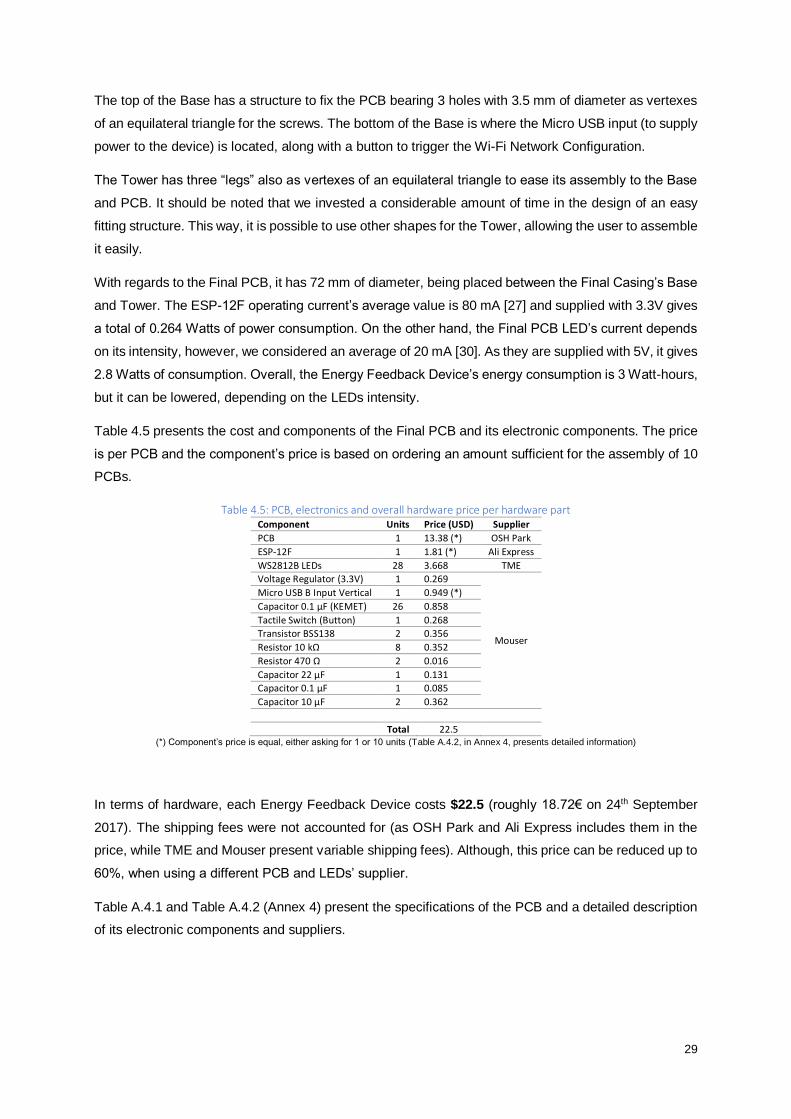
29
The top of the Base has a structure to fix the PCB bearing 3 holes with 3.5 mm of diameter as vertexes
of an equilateral triangle for the screws. The bottom of the Base is where the Micro USB input (to supply
power to the device) is located, along with a button to trigger the Wi-Fi Network Configuration.
The Tower has three “legs” also as vertexes of an equilateral triangle to ease its assembly to the Base
and PCB. It should be noted that we invested a considerable amount of time in the design of an easy
fitting structure. This way, it is possible to use other shapes for the Tower, allowing the user to assemble
it easily.
With regards to the Final PCB, it has 72 mm of diameter, being placed between the Final Casing’s Base
and Tower. The ESP-12F operating current’s average value is 80 mA [27] and supplied with 3.3V gives
a total of 0.264 Watts of power consumption. On the other hand, the Final PCB LED’s current depends
on its intensity, however, we considered an average of 20 mA [30]. As they are supplied with 5V, it gives
2.8 Watts of consumption. Overall, the Energy Feedback Device’s energy consumption is 3 Watt-hours,
but it can be lowered, depending on the LEDs intensity.
Table 4.5 presents the cost and components of the Final PCB and its electronic components. The price
is per PCB and the component’s price is based on ordering an amount sufficient for the assembly of 10
PCBs.
Table 4.5: PCB, electronics and overall hardware price per hardware part Component Units Price (USD) Supplier
PCB 1 13.38 (*) OSH Park
ESP-12F 1 1.81 (*) Ali Express
WS2812B LEDs 28 3.668 TME
Voltage Regulator (3.3V) 1 0.269
Mouser
Micro USB B Input Vertical 1 0.949 (*)
Capacitor 0.1 µF (KEMET) 26 0.858
Tactile Switch (Button) 1 0.268
Transistor BSS138 2 0.356
Resistor 10 kΩ 8 0.352
Resistor 470 Ω 2 0.016
Capacitor 22 µF 1 0.131
Capacitor 0.1 µF 1 0.085
Capacitor 10 µF 2 0.362
Total 22.5 (*) Component’s price is equal, either asking for 1 or 10 units (Table A.4.2, in Annex 4, presents detailed information)
In terms of hardware, each Energy Feedback Device costs $22.5 (roughly 18.72€ on 24th September
2017). The shipping fees were not accounted for (as OSH Park and Ali Express includes them in the
price, while TME and Mouser present variable shipping fees). Although, this price can be reduced up to
60%, when using a different PCB and LEDs’ supplier.
Table A.4.1 and Table A.4.2 (Annex 4) present the specifications of the PCB and a detailed description
of its electronic components and suppliers.

30
Chapter 5: Acquisition of Real Consumption Data
We initiated a campaign to acquire participants, within the Portuguese Residential energy consumers’
population, willing to install a Wi-Fi electric meter’s sensor and provide us with remote access to their
real-time households’ instant consumption power. The participants’ data will be used to create a new
database of Portuguese Residential energy consumption, available for future studies.
In the second phase, we conducted an experiment to assess our device’s ability to provide energy
consumption feedback in a way that would ultimately lead to energy savings. This was executed by
installing our Energy Feedback Device in the participants’ households (see Chapter 8).
This chapter will address the participant acquisition and selection process, the household
characterization parameters and the data structure for the database.
5.1 Campaign
5.1.1 Audience archetypes
Given the innovative nature of the experiment and the large size of the Portuguese Residential energy
consumers’ population, it was necessary to optimize the audience vs. enrolment ratio. Therefore, three
audience archetypes were formulated:
• Archetype I – Portuguese environmental and energy efficiency online communities’ users;
• Archetype II – Engineering students from technological backgrounds;
• Archetype III – Enthusiasts of technological innovation for energy efficiency.
Table 5.1 summarizes the characteristics of each archetype.
Table 5.1: Characteristics of audience archetypes and desired mindset hypothesis
Archetype Age Interests Mindset
I 20-60 Energy efficiency, renewable energies and/or environmental awareness
Conscious mindset towards energy consumption
II 20-30 Technological innovation Better acceptance and adaptability to technological innovations
III 30-60 Technological innovation related to energy efficiency
Able to relate to electricity consumption efficiency on a personal level when compared to Archetype II (i.e., ‘pain’ of electricity costs)
5.1.2 Campaign content
Two types of content presentation were used to recruit participants for the experiment. The Flyer was
used as a first presentation for the audience, while the Infographic presented further information for the
audience interested in applying as a participant.
Figure A.5.1 (Annex 5) presents the images of the Flyer and Infographic. The campaign content, shown
in Table 5.2, intended to reach the audience through promotion channels, addressing the problem to be
solved, as well as providing detailed information about the experiment, experiment, benefits,
requirements and enrolment methods.

31
Table 5.2: Campaign content’s type, provided information and distribution format
Type Information Format
Flyer Problem to be solved, experiment context and available enrolment methods Digital and paper
Infographic Problem to be solved, experiment context, benefits and requirements as a participant Digital
5.1.3 Enrolment methods
Three enrolment methods were prepared for the applicants. The main enrolment method was the
Landing Page, available on Figure A.5.2 (Annex 5). Table 5.3 presents the three methods, the required
fields to be filled in as well as additional information.
Table 5.3: Enrolment methods provided to the audience, required fields and description
Enrolment Method Access Required
Fields Description (how to apply and further information)
Landing Page (with Registration Form)
www.energymonitor.xyz
Name
Fill in Registration Form’s fields and submit. Access detailed information about the experiment through the Infographic
Phone N.
N. Occupants
E-mail goncalo.f.de.andrade
@ulisboa.pt
Name Send an e-mail message with the required fields filled in. Used also as a contact method for further clarification
Phone N.
N. Occupants
Phone/SMS 91 655 645 0
Name Send an SMS or make a phone call to provide the required fields
N. Occupants Legend: N. - Number
5.1.4 Campaign methodology and Timeline of activities
The campaign content reaches the audience through a promotion channel. A conversion is made when
an audience member registers through on of the three aforementioned enrolment methods, becoming
an applicant for the experiment. Figure 5.1 illustrates the campaign methodology.
Figure 5.1: Campaign methodology diagram for applicant’s acquisition
Three types of audience archetypes were associated with three types of channels, resulting in the
creation of three sub-campaigns: Campaign I, II and III. Figure 5.2 presents the timeline of activities
(2016) from the start of the campaign to the final stage – the participant’s stable monitoring.
Figure 5.2: Timeline of the campaign’s activities (2016)

32
5.1.5 Campaign Channels, Promotion and Results
To disseminate the campaign content, it was necessary to define a suitable promotional channel for
each one of the audience archetypes; as such, three channels were defined.
5.1.5.1 Campaign I – Channel I: Energy and Environment Online Communities’ Article
Upon researching Portuguese online communities involved in topics related to the environment, energy
efficiency and renewable energy, we concluded that they were almost non-existent or inactive.
Furthermore, they were usually governmental entities sponsored by European Union funds.
We needed to contact these communities’ administrators in order to reach the Audience Archetype I.
Table A.5.1 (Annex 5) presents the information about the 13 websites, apparently active, that were
approached. On March 2016, we contacted these online communities, via e-mail, presenting the context
of this work and requesting the promotion of the campaign on their website through the Flyer. The flyer
itself was provided in digital format over e-mail.
The only answer came from DECO, which scheduled a meeting at their headquarters to discuss the
scope of the campaign. After the meeting, the campaign content was posted on DECO’s portal for
renewable energies (https://energias-renovaveis-emcasa.pt), available in Figure A.5.3 (Annex 5).
This campaign was promoted for a period of two months, ultimately resulting in only one applicant.
Therefore, due to the insignificant number of registrations, Campaign I was abandoned, arousing the
need of resorting to Campaign II and III to recruit participants for the experiment.
5.1.5.2 Campaign II – Channel II: E-mail to Engineering Students
We started by targeting Electrical and Computer Engineering students, from Instituto Superior Técnico,
as the first hypothesis for Audience Archetype II. Student delegates were used to promote the campaign
via e-mail. We created an e-mail script to be addressed to the students, containing information about
the campaign and presenting the Landing Page (http://www.energymonitor.xyz), with the Registration
Form (enrolment method) and Infographic (containing the campaign’s content).
At the end of May 2016, we contacted, via e-mail, the students’ delegates with information regarding the
purpose of the campaign as well as the e-mail script to be sent to the students. This campaign was
promoted for three weeks, resulting in 61 applicants.
5.1.5.3 Campaign III – Channel III: Personal Contact
The identification of subjects from the Audience Archetype III was made using the investigator’s own
contact network, either by direct identification – whereby the investigator identified a previously known
subject — or by indirect identification – whereby someone from the contact network indicated a
suitable subject to be approached. The campaign’s content and enrolment methods were presented via
conversation and a printed Flyer was also provided to the subjects. This campaign was promoted for
one month, resulting in 10 applicants.

33
5.2 Selection of Participants and sensor’s installation
5.2.1 Selection Process
Campaign II and III culminated in a total of 71 applicants. These applicants would further be vetted
down, as we only had 7 electric meters’ sensors available for the experiment. To avoid potential
problems and setbacks, upon the installation of the sensor, we started by defining three exclusion
parameters for the participant’s selection: 1) Does not have Wi-Fi access at the electric meter’s location;
2) Does not have an electric socket near the meter, or any means for supplying power to the sensor;
3) Does not have a digital electric meter.
Any applicant with one of the three exclusion parameters did not proceed to the final selection stage, as
we wanted to select the applicants with the optimal conditions for the sensor’s installation. Table 5.4
presents the Installation Conditions’ parameters, employed to create a survey (http://bit.ly/2pGCTwW),
to be filled in by the applicants. This survey contained the three exclusion parameters as well as
additional parameters to evaluate the applicants’ suitability for the experiment.
Table 5.4: Installation Conditions’ parameters and description
Parameters Description
Household Type Familiar or Non-familiar
Occupants Number of occupants in the household
Electric Meter (*) Analog or digital
Meter Location Inside/outside household and inside/outside electrical switchbox
Wi-Fi Access (*) Availability of a Wi-Fi network at the meter’s location
Powering Sensor (*) Availability of a means to power the sensor, using an electric socket near the meter (*) – Exclusion Parameters
For the 61 applicants of Campaign II, we sent an e-mail with the Installation Conditions’ survey and 23
of them answered. The answers were analysed and only 8 applicants were chosen to proceed to the
final selection stage. For the 10 applicants of Campaign III, their Installation Conditions’ parameters
were obtained via personal contact; although, only 6 applicants met the conditions to proceed to the
final selection stage.
We now had a total of 14 potential candidates with suitable conditions to undergo installation of the
electric meters’ sensors. However, only 7 could be selected to become participants. We sent an e-mail
to the remaining 14 applicants announcing their suitability to receive the sensor. The final group of 7
participants were selected based on the order of arrival of the e-mail replies. Table A.5.5 (Annex 5)
summarizes the overall process (number of subjects for each campaign’s stage).
5.2.2 Sensor configuration, installation and troubleshooting
Figure 5.3 presents the electric meter’s sensor used and its placement on a digital electric meter.
Figure 5.3: EnergyOT Optic Sensor (left) and Digital Energy Meter indicating the meter’s LED (right)
34
We used the sensor brand-named EnergyOT Optic, from EnergyOfThings (www.eot.pt). It is a Wi-Fi
Electric Meter Sensor “to be used with digital energy meters” and able to send the instant power
consumption data of the household to the cloud in real-time (namely, with a “resolution up to 15s”).
To access the energy data, it was necessary to create an account on https://my.eot.pt. We created an
account for each participant, providing the number of impulses/kWh of their meter to obtain accurate
power readings.
Their Wi-Fi credentials were requested and, prior to receiving the sensor, each participant had it
configured for the desired Wi-Fi network and connected with their on-line account. In order to install the
sensor on the digital electric meter (right side of Figure 5.3), the participant must place the “Photodiode”
of the sensor centred with the meter’s LED to obtain accurate readings.
To supply power to the sensor, a Micro USB Transformer must be used, by plugging it into the nearest
electrical socket and connecting a USB cable to the power input of the sensor. With regards to technical
problems, participants had some issues with the initial monitoring stage, mainly due to the photodiode:
(1) cable tension between the sensor’s box and photodiode loosened the photodiode from the meter;
(2) lack of centring between the photodiode and the meter’s LED upon installation led to incorrect
power readings. The problems were identified, and solutions provided. Only one of the participant’s
sensor was replaced due to the malfunctioning of the photodiode.
5.3 Creation of a Database of Household Consumption Data
We will present the features used to characterize the participants and their households, as well as the
data structure used to collect and save their raw consumption data.
5.3.1 Household Characterization
This section presents the features that characterize each household, its occupancy, electricity supply
contract and main appliances. These features remained mostly unchanged during the data collection
period.
We created a survey to be filled in by the participants (available on http://bit.ly/2qB83ss), divided into
two parts. The participants’ answers to the survey will be presented and explored on Chapter 8.
Table 5.6 presents the features contained on the first part of the survey. Table 5.7 presents the
appliances, presented as a multiple-choice survey, used for the second part. This framework was based
on J. Abreu [31] work, whereby technical questions in were simplified (e.g., not requesting building area)
to be easier when filled in by the participant.
Table 5.6: Characteristics of the household, occupancy and electricity supply contract Features Description
Household type Familiar – occupants are family members; Non-Familiar – occupants are not family members
Number of occupants Number of people living on the household
Building Type Apartment or House
Number of rooms Number of separate bedrooms (i.e., to provide a notion of the household’s dimension)
Contracted power (kVA) Household’s contracted power, in kVA (kilovolt-ampere)
Tariff regime Household’s contracted tariff regime – simple, bi-hourly, or tri-hourly

35
Table 5.7: Categories and appliances – multiple-choice survey
Category Appliances (options)
Heating and Cooling Sources Water Heater Elect. Heater Air Conditioning Fan Heater
Oil-filled Heater Air Cooler Ventilator Fans
Kitchen Elect. Stove Induction Cooker Elect. Oven Elect. Fryer
Elect. Grill Microwaves Elect. Kettle Coffee Machine
Laundry and Food Coolers Dishwasher Washer Dryer Fridge
Fridge-Freezer Freezer Legend: N. – Number; Elect. – Electric
5.3.2 Household Consumption Data Structure
This section presents the structure of the database that stores the consumption data for each one of the
participants’ household. We proposed a format that can be used not only in the scope of the current
work, but also for future studies that can benefit from the raw data collected.
The participant’s daily monitoring data (Daily Data File) was saved inside each participant’s folder, on a
CSV file, named according to the date of the day (year-month-day.csv). Each Daily Data File had four
fields: ID – sample’s identifier number; Time – using Lisbon’s time zone; Power – power value, in Watts,
or “-1” for missing samples; and Temperature – temperature in Celsius.
For each participant’s sensor, a unique API (Application Programming Interface) Key was assigned,
allowing remote access to the last power value registered by their sensor. To obtain Lisbon’s current
temperature, we used the Web API of a Weather Service (www.wunderground.com).
Using these sources, a Python script (called Gatherer) was created for each participant. It requested
the temperature and power value within 35-second intervals and inserted them into the Daily Data File.
The initial monitoring started at the end of August; however, the Gatherer was developed, tested and
implemented during September 2016. It started to collect stable data on October 2016. The overall
Energy Data System is presented on Chapter 7.
5.4 Conclusion
We created a campaign and collected 7 residential energy consumers, as the participants of our
experiments. We found that Portuguese online communities related to energy efficiency, environment
and renewable energies are almost inexistent or inactive, therefore, they are not suitable for the
acquisition of participants. On the other hand, we found that technology enthusiasts are easier to find
and willing to enrol as participants. In this first part of the experiment, we installed Wi-Fi electric meter’s
sensors on their households to remotely monitor their energy consumption. Moreover, we created a
framework based on [31] to characterize the households of the participants.
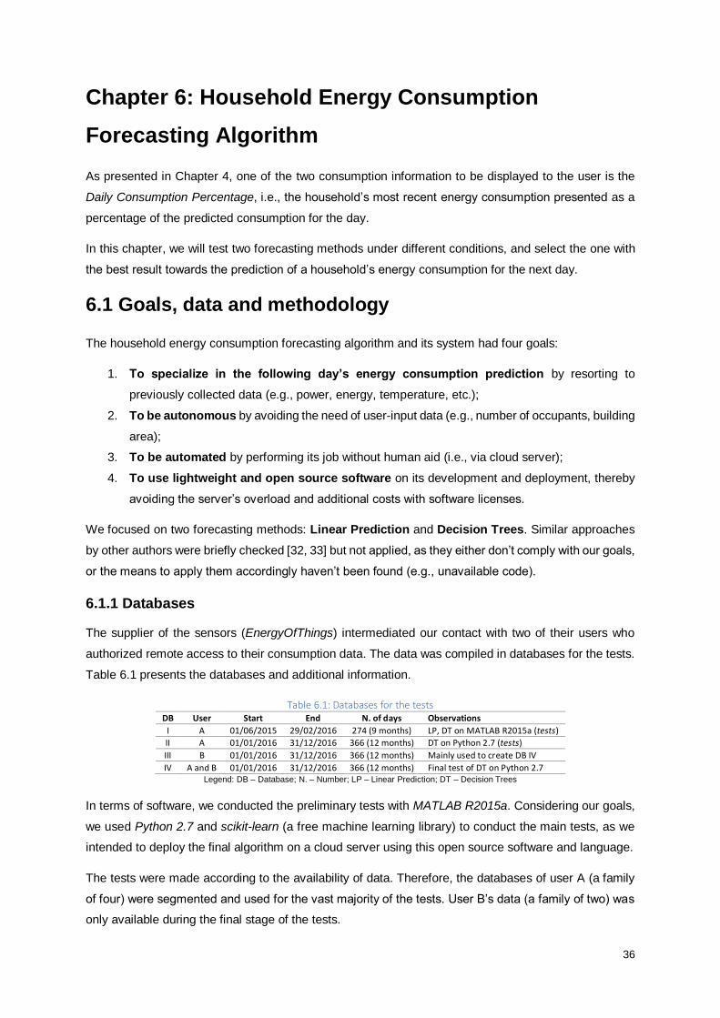
36
Chapter 6: Household Energy Consumption
Forecasting Algorithm
As presented in Chapter 4, one of the two consumption information to be displayed to the user is the
Daily Consumption Percentage, i.e., the household’s most recent energy consumption presented as a
percentage of the predicted consumption for the day.
In this chapter, we will test two forecasting methods under different conditions, and select the one with
the best result towards the prediction of a household’s energy consumption for the next day.
6.1 Goals, data and methodology
The household energy consumption forecasting algorithm and its system had four goals:
1. To specialize in the following day’s energy consumption prediction by resorting to
previously collected data (e.g., power, energy, temperature, etc.);
2. To be autonomous by avoiding the need of user-input data (e.g., number of occupants, building
area);
3. To be automated by performing its job without human aid (i.e., via cloud server);
4. To use lightweight and open source software on its development and deployment, thereby
avoiding the server’s overload and additional costs with software licenses.
We focused on two forecasting methods: Linear Prediction and Decision Trees. Similar approaches
by other authors were briefly checked [32, 33] but not applied, as they either don’t comply with our goals,
or the means to apply them accordingly haven’t been found (e.g., unavailable code).
6.1.1 Databases
The supplier of the sensors (EnergyOfThings) intermediated our contact with two of their users who
authorized remote access to their consumption data. The data was compiled in databases for the tests.
Table 6.1 presents the databases and additional information.
Table 6.1: Databases for the tests DB User Start End N. of days Observations
I A 01/06/2015 29/02/2016 274 (9 months) LP, DT on MATLAB R2015a (tests)
II A 01/01/2016 31/12/2016 366 (12 months) DT on Python 2.7 (tests)
III B 01/01/2016 31/12/2016 366 (12 months) Mainly used to create DB IV
IV A and B 01/01/2016 31/12/2016 366 (12 months) Final test of DT on Python 2.7 Legend: DB – Database; N. – Number; LP – Linear Prediction; DT – Decision Trees
In terms of software, we conducted the preliminary tests with MATLAB R2015a. Considering our goals,
we used Python 2.7 and scikit-learn (a free machine learning library) to conduct the main tests, as we
intended to deploy the final algorithm on a cloud server using this open source software and language.
The tests were made according to the availability of data. Therefore, the databases of user A (a family
of four) were segmented and used for the vast majority of the tests. User B’s data (a family of two) was
only available during the final stage of the tests.

37
6.1.2 Training, Validation and Test Set
To apply a coherent method for the results’ validation, DB II, III and IV, comprising one year of data,
were divided into a training, validation and test set. These three sets are widely used in information
science to find and confirm predictive relationships from data. Their definitions are given below:
1. Training Set (50% of the year): set of data used to discover potentially predictive relationships
used for learning to fit the parameters [34].
2. Validation Set (30% of the year): set of data used to tune the parameters and check the results
of the Training Set [34].
3. Test Set (20% of the year): set of data used to assess the strength and utility (i.e., performance)
of a predictive relationship, by checking the Training and Validation Set’s results [34].
The days of the DBs were assigned to each set in a way that would not favour any season of the year.
Table A.6.1, in Annex 6, exemplifies the assignment method for the first 10 days of a year, being this
method repeatedly employed until the end of the year for DB II, III and IV.
6.1.3 Experimental system methodology
Figure 6.1 presents the system employed for the tests of the forecasting algorithm, following a structure
similar to the Energy Data System (see Chapter 7).
Figure 6.1: Simplified diagram of the experimental system methodology
The Historical Data contained raw data (e.g., energy, power, temperature, etc.) for each day of the
year. Due to the electric meter’s sensor monitoring failures, the DBs had invalid days. The Filter
identified them, replaced their missing data and saved the information in the Treated Historical Data –
containing the daily variables presented in Table A.6.2 (Annex 6). Table A.6.3 (Annex 6) presents the
number of valid days of DB II and III for their Validation, Training and Test set.
Each test had specific Parameters related to the amount and type of past data to be used, as well as
to the parameters employed on the forecasting algorithm. According to them, the Extractor computed
the Train Dataset to be used by the Forecaster, which in turn provides the predictions under the defined
parameters. Table A.6.4, in Annex 6, presents variables of the Train Dataset.
Finally, for each day, the Error process computes the difference between the real and predicted energy
consumption. The mean absolute error was calculated for each test by using only valid days (i.e., days
without missing monitoring data due to the sensor’s failures). Greedy algorithm was employed to define
the next tests’ conditions based on the mean absolute error results of previous tests.

38
The greedy algorithm is an algorithmic strategy that employs the heuristic technique of making the
locally optimal choice at each stage with the hope of finding a global optimum. In other words, it is taking
the best immediate, or local, solution to speed up the process of finding an answer for the globally
optimal solution [35].
A common way of evaluating a forecast error is by its mean absolute error (MAE), which is a measure
of the difference between two continuous variables [36]. The MAE is presented in equation 6.1, where
𝐴𝑛 is the real value, 𝐹𝑛 is the forecasted value and 𝑁 is the total number of values.
𝑀𝐴𝐸 =∑ |𝐹𝑛 − 𝐴𝑛|𝑁
𝑛=1
𝑁 (6.1)
6.2 Linear Prediction Forecasting Algorithm
Linear prediction is a mathematical operation, where future values of a discrete-time signal are
estimated as a linear function of previous samples [37]. It is usually given by the equation:
𝑥(𝑛) = ∑ 𝛼𝑘 ∗ 𝑥(𝑛 − 𝑘)
𝑁
𝑘=1
(6.2)
In 6.2, 𝑥(𝑛) is the value of the predicted signal, 𝑥(𝑛 − 𝑘) the previous observed values, 𝑁 the number
of previous values, and 𝛼𝑘 the predictor coefficients [37]. In our case, we used 𝑥 = 𝑊 to denote energy.
We will modify the original equation to test two hypotheses. Table 6.2 presents each equation, where:
𝑵 – number of previous days; 𝑲’ – interval between previous days; and ∆𝑳𝑷𝑪(𝒏) – interval of previous
days for the predictor coefficients computation.
Table 6.2: Linear Prediction - Summary of Hypotheses I and II Hyp. Equation Conditions and information
I 𝐼(𝑛) = ∑1
𝑁∗ 𝑊(𝑛 − 𝑘 ∗ 𝐾′) 𝑁
𝑘=1 (6.3)
Coefficients are not computed (𝛼𝑘 =1
𝑁)
Tests 𝐾’ from 1 to 7 𝑁 from 1 to 20
Objective What is the best 𝐾’ vs. 𝑁 combination?
II 𝐼𝐼(𝑛) = ∑ 𝛼𝑘 ∗ 𝑊(𝑛 − 𝑘 ∗ 𝐾′)𝑁𝑘=1 (6.4)
Coefficients (𝛼𝑘) are computed, therefore, ∆𝐿𝑃𝐶(𝑛) is introduced
Tests 𝐾’ from 1 to 7 9 ∆𝐿𝑃𝐶(𝑛) Vary 𝑁 according to ∆𝐿𝑃𝐶
Objective What is the best 𝐾’ vs. 𝑁 vs. ∆𝐿𝑃𝐶(𝑛) combination? Legend: Hyp. - Hypothesis
In both hypotheses, we intended to find out if the use of non-consecutive previous days (𝐾′ ≠ 1) perform
better predictions. We also tested several combinations of 𝑲’ vs. 𝑵, using MAE to find the best.
Hypothesis I (6.3) is a simple average while Hypothesis II (6.4) is a weighted average, which predictor
coefficients are computed by MATLAB’s 𝑙𝑝𝑐 𝑓𝑢𝑛𝑐𝑡𝑖𝑜𝑛. The quality of the computed coefficients is
dependent on the interval of previous days provided to the function. Therefore, we tested 9
∆𝑳𝑷𝑪(𝒏) varying the 𝑵 accordingly.
We resorted to DB I, using its 134 valid days for the MAE computation in order to appropriately compare
the results among the different tests.

39
6.2.1 Hypothesis I
Table 6.3 presents the MAE results for Hypothesis I (6.3) with 𝐾’ ranging from 1 to 7 and 𝑁 from 1 to
14. The greener boxes represent smaller MAE values while the redder boxes represent higher values.
Table 6.3: Linear Prediction – Hypothesis I – Mean Absolute Error results (in kWh) 𝑵 (number of previous days)
1 2 3 4 5 6 7 8 9 10 11 12 13 14
𝑲′ (
inte
rval
bet
we
en
pre
vio
us
day
s)
1 3.261 2.984 2.932 2.931 2.927 2.971 2.961 2.951 2.941 2.963 2.976 2.983 2.986 2.950
2 3.660 3.259 3.172 3.114 3.096 3.082 3.020 3.033 3.072 3.144 3.190 3.179 3.191 3.158
3 3.907 3.509 3.336 3.301 3.320 3.307 3.308 3.273 3.286 3.267 3.291 3.286 3.292 3.306
4 3.943 3.495 3.350 3.282 3.352 3.293 3.267 3.258 3.257 3.267 3.261 3.287 3.310 3.327
5 3.986 3.625 3.568 3.610 3.466 3.369 3.329 3.358 3.392 3.434 3.447 3.477 3.543 3.646
6 4.056 3.675 3.571 3.455 3.393 3.375 3.395 3.429 3.423 3.470 3.595 3.737 3.867 3.967
7 3.796 3.529 3.313 3.327 3.302 3.391 3.408 3.415 3.532 3.683 3.814 3.948 4.136 4.361
The best combination was found when using the 5 previous consecutive days’ energy consumption
data (𝐾’ = 1 and 𝑁 = 5) to predict the following day, with an MAE of 2.927 kWh.
In general, the best prediction results were found for 5 ≤ 𝑁 ≤ 10. We also found that the use of
previous consecutive days (𝐾’ = 1) led to MAE results inferior to 3 kWh, which did not happen for the
rest of the 𝐾’ values tested, i.e., for the use of non-consecutive previous days.
6.2.2 Hypothesis II
Table 6.4 presents the values of ∆𝐿𝑃𝐶(𝑛) and the associated 𝑁 values for the 9 experiments conducted.
Table 6.4: Linear Prediction – Hypothesis II – 9 experiments for the tests of ∆LPC vs. N Experiment 1 2 3 4 5 6 7 8 9
∆𝑳𝑷𝑪(𝒏) 1: 𝑛-1 𝑛-7: 𝑛-1 𝑛-14: 𝑛-1 𝑛-21: 𝑛-1 𝑛-28: 𝑛-1 𝑛-30: 𝑛-1 𝑛-37: 𝑛-1 𝑛-44: 𝑛-1 𝑛-51: 𝑛-1
𝑵 1 to 20 1 to 7 1 to 14 1 to 21 1 to 28 1 to 30 1 to 37 1 to 44 1 to 51
The ∆𝑳𝑷𝑪(𝒏) is a dynamic window – considering each day, 𝑛 – to allocate its interval. 𝑁 represents the
number of previous days used as well as the number of coefficients computed by the 𝑙𝑝𝑐 𝑓𝑢𝑛𝑐𝑡𝑖𝑜𝑛.
Therefore, 𝑁 must have an interval of values which size is smaller than its ∆𝐿𝑃𝐶(𝑛) interval.
We tested 𝐾’ from 1 to 7 and 𝑲’ = 𝟏 presented the best results. Table 6.5 presents the results for the
9 ∆𝐿𝑃𝐶(𝑛) intervals and for 𝑁 (from 1 to 10), when using 𝐾’ = 1 (previous consecutive days). The
greener boxes represent smaller MAE values and the redder ones represent higher values.
Table 6.5: Linear Prediction – Hypothesis II – Mean Absolute Error results (K’=1) 𝑵 (number of previous days)
1 2 3 4 5 6 7 8 9 10
∆𝑳
𝑷𝑪
(𝒏)
(in
terv
al f
or
the
αk
com
pu
tati
on
)
𝟏: 𝒏-𝟏 3.278 3.006 3.024 3.073 3.085 3.129 3.140 3.194 3.243 3.293
𝒏-𝟕: 𝒏-𝟏 4.508 4.836 5.287 6.042 6.679 7.429 8.074 - - -
𝒏-𝟏𝟒: 𝒏-𝟏 3.639 3.749 4.011 4.334 4.635 4.926 5.203 5.402 5.693 6.080
𝒏-𝟐𝟏: 𝒏-𝟏 3.430 3.405 3.599 3.868 4.073 4.313 4.532 4.831 5.052 5.331
𝒏-𝟐𝟖: 𝒏-𝟏 3.364 3.292 3.496 3.682 3.824 4.012 4.178 4.383 4.574 4.815
𝒏-𝟑𝟎: 𝒏-𝟏 3.343 3.229 3.384 3.567 3.710 3.896 4.074 4.277 4.405 4.673
𝒏-𝟑𝟕: 𝒏-𝟏 3.313 3.162 3.286 3.461 3.569 3.713 3.860 4.056 4.193 4.386
𝒏-𝟒𝟒: 𝒏-𝟏 3.298 3.116 3.226 3.373 3.470 3.603 3.745 3.929 4.031 4.200
𝒏-𝟓𝟏: 𝒏-𝟏 3.290 3.056 3.160 3.310 3.410 3.532 3.668 3.818 3.908 4.048
The best result was found for ∆𝑳𝑷𝑪(𝒏) = 𝟏: 𝒏-𝟏 and 𝑵 = 𝟐 (for 𝑲’ = 𝟏) with a MAE of 3.006 kWh.

40
Therefore, the prediction coefficients computed by MATLAB’s 𝑙𝑝𝑐 𝑓𝑢𝑛𝑐𝑡𝑖𝑜𝑛 are better when using all the
previous samples of day, 𝑛, as the interval for their computation. Along with it, the use of the two previous
consecutive days led to the best result.
For 𝑁 ≥ 3 the MAE increases, therefore, the increase of the number of previous days used for
prediction led to worse predictions. Most of the tests present their smallest error on 𝑁 = 2, i.e., using
the energy values of the two previous consecutive days along with their two predictor coefficients to
forecast the next day’s energy consumption. Finally, from the 𝐾’ tests (from 1 to 7), we concluded that
the use of previous consecutive days (𝐾’ = 1) led to the best results.
6.2.3 Brief overview
Resorting to DB I data, we can conclude that Hypothesis I (smallest MAE – 2.927 kWh) provides better
results than Hypothesis II (smallest MAE – 3.006 kWh). Therefore, the Linear Prediction Forecasting
Algorithm is given by:
𝐼(𝑛) = ∑1
𝑁∗ 𝑊(𝑛 − 𝑘)
𝑁
𝑘=1
(6.5)
We used (6.5) – a modification of (6.3) based on the tests’ results – for DB II’s Training Set, varying the
𝑁 for multiples of 7 (i.e., weeks) and for a set of values smaller than 7. Table 6.6 presents the tested
values and their MAE results.
Table 6.6: Equation 6.2 – Mean Absolute Error results (DB II Training Set) N 4 5 6 7 14 21 28
MAE 2.977 2.934 2.887 2.801 2.920 2.861 2.910
The best result was found for 𝑁 = 7, with an MAE of 2.801 kWh for DB II’s Training Set. For this case,
DB II’s Validation and Test Set MAE is 2.588 kWh and 2.665 kWh, respectively. These values will be
used as a baseline for the tests of the Decision Trees’ algorithm.

41
6.3 Decision Trees Forecasting Algorithm
Decision trees are nonparametric supervised learning methods used for classification and regression
[38]. The objective is to reach to a model that predicts the value of the target variable by learning decision
rules from the input data features [38].
The method uses a dataset with input data features and their associated target values to train a model,
creating a tree-like graph. The predictive model goes from observations about an item, i.e., the input
data features – represented in the nodes – to a conclusion about the item’s target value – represented
in the leaves [38, 39]. Data comes in records of the form: (𝒙, 𝒀) = (𝒙𝟏, 𝒙𝟐, 𝒙𝟑, … , 𝒙𝒌, 𝒀). The dependent
variable, 𝒀, is the target variable that we are trying to understand [39]. The vector 𝒙 is composed of the
input variables 𝑥1, 𝑥2, 𝑥3, … , that are used for that task [39]. The Decision Trees encompasses several
methods of forecasting. Therefore, we selected the following three methods to be tested:
Regression trees are employed to predict real numbers, such as energy consumption, using the
previously described methodology (on the other hand, classification trees are employed to predict the
class where the target variable belongs to, i.e., discrete values) [39].
Random forests, proposed by Breiman in 2001 [40], are an ensemble learning method that constructs
a large group of regression trees (in our case) at training time and outputs the mean prediction of the
individual trees.
Extremely Randomized Trees, proposed by P. Geurts in 2006 [41], have further randomization when
compared to Random Forests. They are trained as Random Forests, using bagging and the random
subspace method. However, the top-down splitting in the tree learner is randomized. In alternative to
computing the locally optimal data feature vs. split combination for each feature, by Gini impurity or
information gain, a random value is selected for the split. This value is selected from the feature’s
empirical range in the tree’s Training Set (i.e., bootstrap sample).
6.3.1 Objectives, resources and evaluation
During the development of the Decision Trees’ forecasting algorithm, we defined four objectives:
I) To determine the number of days used for the training period, by testing different training
periods and comparing their MAE results.
II) To select the forecasting method (Regression Tree, Random Forests or Extremely
Randomized Trees), by testing them under the same conditions and comparing their MAE
results.
III) To find the set of pre-pruning parameters that leads to the smallest MAE, by testing different
values and resorting to greedy algorithm to decide following tests’ conditions.
IV) To find the number and type of input variables that leads to the smallest MAE, by testing
several combinations and utilizing greedy algorithm to perform decisions.
Due to DB II’s data unavailability at the time of the test, we resorted to DB I (User A) to determine the
number of previous days used for the training period and to compare, for the first time, the prediction

42
performance between Linear Prediction and Decision Trees. As a baseline, we employed the smallest
Linear Prediction MAE found for DB I, with a value of 2.927 kWh (see Section 6.2.1).
Upon DB II’s availability (User A), the data was used to determine the best values for the remaining
objectives. As a baseline, we used the smallest MAE found for DB II’s Training Set, with a value of 2.801
kWh (see Section 6.2.3).
DB III (User B) was only available during the final stage of the tests, being briefly used to confirm
previous assumptions over the input variables. DB IV, containing data of both DB II and III, was
employed during the last test to determine the number and type of input variables.
6.3.2 Objective I: Number of days used for the training period
We resorted to DB I data to determine the number of previous days used to train the Decision Trees’
algorithm. We employed the same 134 days, as on Linear Prediction, to compare the MAE results.
We applied MATLAB’s 𝑓𝑖𝑡𝑟𝑡𝑟𝑒𝑒(𝑥, 𝑦) function, which returns a Regression Tree, based on the input
variables x and output y. In our case, the output is the energy consumption for the day n, 𝑊(𝑛). We
conducted two experiments using two different sets of input variables.
• Experiment 1 – input variables: day of the week, yesterday’s energy consumption and
yesterday’s mean temperature [𝐷𝑎𝑦(𝑛), 𝑊(𝑛 − 1), 𝑇𝑚𝑒𝑑(𝑛 − 1)].
• Experiment 2 – input variables: yesterday’s minimum power, energy consumption and mean
temperature [𝑃𝑚𝑖𝑛(𝑛 − 1), 𝑊(𝑛 − 1), 𝑇𝑚𝑒𝑑(𝑛 − 1)].
Each set of input variables creates a 3-variable regression tree, trained under a certain number of
previous days, as the training period, to predict the following day’s energy consumption. Table 6.7
presents the MAE results for each experiment’s training periods (in multiples of 7, i.e., weeks).
Table 6.7: Decision Trees – Objective I – Mean Absolute Error results (DB I)
Training Period (days)
7 14 21 28 35 42 49
Experiment 1 3.071 2.946 2.967 2.913 3.066 3.113 3.151
Experiment 2 3.096 2.958 2.972 2.922 3.074 3.156 3.184
The best results were obtained when 28 days of training data was used to predict the following
day – experiment 1 (2.913 kWh) and experiment 2 (2.922 kWh). These values present a smaller error
when compared with DB I’s Linear Prediction smallest MAE (2.927 kWh).
In some machine learning cases, the use of a larger training period provides better predictions. Google's
Research Director, Peter Norvig, was quoted saying that "We don’t have better algorithms. We just have
more data”. This quote is usually linked to the article on "The Unreasonable Effectiveness of Data", co-
authored by Norvig himself [42]. In our case, the consumption varies along the year, according to the
season or unexpected user behaviour (e.g., vacation). The use of 28 previous days presented the best
results in our data. Consequently, it was selected as the number of days used for the training period of
the Decision Trees’ algorithm.

43
6.3.3 Objective II: Forecasting method
We resorted to DB II’s Training Set to select the best forecasting method. The three Decision Trees’
forecasting methods were tested under the same set of pre-pruning parameters and input variables,
comparing their MAE results, to select the one with the best prediction performance. We also took
advantage of the usage of pre-pruning parameters to understand their influence on the avoidance of
underfitting and overfitting.
Overfitting is one of the main difficulties of forecasting methods. This happens when prediction models
continue to apply hypotheses that reduce training error at the cost of an increased test error. There are
two ways to avoid it [43]: pre-pruning – stop growing the tree before it perfectly classifies the Training
Set; and post-pruning – allows the tree to perfectly classify the Training Set, and then post prune the
tree.
The Decision Trees’ forecasting functions, from Python’s machine learning library (scikit-learn) [44], do
not have post-pruning capabilities. Nevertheless, it is possible to change their pre-pruning parameters’
values. In Annex 6, Table A.6.5 presents each function’s default values for these parameters and Table
A.6.6 presents their definition.
We created two experiments for objective II based on two different sets of input variables. In each
experiment’s test, we assigned a set of pre-pruning parameters and apply them to the 3 functions. Then,
their MAE results for the next day’s energy consumption prediction were compared. When choosing
the next set of parameters, greedy algorithm was employed as we discover combinations and values
that led to better MAE results. Table 6.8 presents the two experiments’ information.
Table 6.8: Decision Trees - Objective II – conditions of experiment 3 and 4 (DB II) Experiment 3 Experiment 4
Input variables 𝐷𝑎𝑦(𝑛), 𝑊28(𝑛), 𝑇𝑚𝑖𝑛(𝑛 − 1) (*) 𝐷𝑎𝑦(𝑛), 𝑊7(𝑛), 𝑇𝑚𝑖𝑛(𝑛 − 1) (*)
Number of tests 55 25
Functions DecisionTreeRegressor vs. RandomForestRegressor vs. ExtraTreesRegressor
Pre-pruning parameters Variable - the same set is experimented on the 3 functions (*) Table A.6.4, in Annex 6, presents the description of each input variable
Experiment 3: Extremely Randomized Trees presented a better prediction performance, when
compared to the results of the other two methods. Table A.6.7 (Annex 6) lists the 16 tests with the best
MAE results, all associated to the ExtraTreesRegressor function.
Experiment 4: Once again, the Extremely Randomized Trees presented the best results. When
compared to the Linear Prediction’s baseline (MAE of 2.801 kWh) only ExtraTreesRegressor presented
smaller MAE results, achieving the value of 2.708 kWh. This is shown in Table A.6.8 (Annex 6), also
comparing with Regression Tree’s results (second-best function).
Using the greedy algorithm, these tests allowed us to gain a deeper understanding by finding two
important pre-pruning parameters from the trees construction. The first parameter is the maximum
number of leaf nodes, 𝒎𝒂𝒙𝑳𝒏𝒐𝒅𝒆𝒔 , to avoid overfitting; and the second parameter is the minimum number
of samples required to be at a leaf node, 𝒎𝒊𝒏𝑺𝑳𝒏𝒐𝒅𝒆𝒔, to avoid underfitting.

44
In terms of pre-pruning parameters, the best results were obtained for a maximum number of leaf nodes
between 2 and 9, along with a minimum of 5 samples per leaf node and the use of mean absolute error
as the criterion to measure the quality of a split (𝟐 ≤ 𝒎𝒂𝒙𝑳𝒏𝒐𝒅𝒆𝒔 ≤ 𝟗, 𝒎𝒊𝒏𝑺𝑳𝒏𝒐𝒅𝒆𝒔= 𝟓 and 𝒄𝒓𝒊𝒕𝒆𝒓𝒊𝒐𝒏 =
𝑴𝑨𝑬).
In terms of forecasting method, we selected the Extremely Randomized Trees due to its superior
performance compared to the Regression Tree and Random Forests.
6.3.4 Objective III: Pre-pruning parameters
We resorted to DB II data to find the best values for the pre-pruning parameters. We also tested the
increase of the number and type of input variables by creating 1-variable to 13-variable Extremely
Randomized Trees.
We employed again the greedy algorithm, but this time to select the combination of variables. We started
with 24 trees of 1-variable, using one of each of the 24 input variables available. The variable with the
smallest MAE was set. Then, 2-variable trees were generated using the remaining 23 variables in the
second position. The 2-variable combination with the smallest MAE was chosen. This process was
repeated until 13-variable Extremely Randomized Trees.
From the findings of 6.3.3 and further analyses to its tests from the pre-pruning parameters’ perspective,
we found that 𝟒 ≤ 𝒎𝒂𝒙𝑳𝒏𝒐𝒅𝒆𝒔 ≤ 𝟖 were associated to the best predictions while maintaining 𝒎𝒊𝒏𝑺𝑳𝒏𝒐𝒅𝒆𝒔=
𝟓 and 𝒄𝒓𝒊𝒕𝒆𝒓𝒊𝒐𝒏 = 𝑴𝑨𝑬.
Two experiments were conducted. During experiment 5, we varied 𝒎𝒂𝒙𝑳𝒏𝒐𝒅𝒆𝒔 from 4 to 8, maintaining
𝒎𝒊𝒏𝑺𝑳𝒏𝒐𝒅𝒆𝒔= 𝟓 and 𝒄𝒓𝒊𝒕𝒆𝒓𝒊𝒐𝒏 = 𝑴𝑨𝑬. Using DB II’s Training Set, we constructed Extremely
Randomized Trees (from 1 to 13 variables) using greedy algorithm to select the next variable for the
combination. During experiment 6, we varied the pre-pruning parameters around the values found for
experiment 5. Using DB II’s Training and Validation Set and 6 random input variables, we created 6-
variable Extremely Randomized Trees for each set of parameters in test, evaluating their MAE.
Experiment 5
Table 6.9 presents the MAE results when varying the pre-pruning parameter 𝒎𝒂𝒙𝑳𝒏𝒐𝒅𝒆𝒔 (4 to 8) for each
combination of the trees’ input variables (1 to 13), while maintaining 𝒎𝒊𝒏𝑺𝑳𝒏𝒐𝒅𝒆𝒔= 𝟓 and 𝒄𝒓𝒊𝒕𝒆𝒓𝒊𝒐𝒏 =
𝑴𝑨𝑬. The type of the assigned variables, for each combination, are shown in Table A.6.9 (Annex 6).
Table 6.9: Decision Trees – Objective III – Mean Absolute Error results of experiment 5 (DB II)
𝒎𝒂𝒙𝑳𝒏𝒐𝒅𝒆𝒔 Number of input variables of Extremely Randomized Trees
1 2 3 4 5 6 7 8 9 10 11 12 13
4 2.816 2.711 2.634 2.603 2.573 2.583 2.527 2.558 2.551 2.534 2.526 2.527 2.524
5 2.814 2.702 2.658 2.608 2.571 2.561 2.556 2.566 2.554 2.574 2.579 2.557 2.539
6 2.809 2.715 2.630 2.571 2.564 2.555 2.539 2.548 2.530 2.540 2.530 2.539 2.556
7 2.815 2.722 2.656 2.575 2.567 2.559 2.560 2.557 2.548 2.552 2.541 2.540 2.529
8 2.813 2.699 2.641 2.598 2.554 2.554 2.550 2.553 2.565 2.577 2.559 2.552 2.549
The best result was found for 𝒎𝒂𝒙𝑳𝒏𝒐𝒅𝒆𝒔 = 𝟒 and 13 variables combination with an MAE of 2.524
kWh. The second best was also found for 𝒎𝒂𝒙𝑳𝒏𝒐𝒅𝒆𝒔 = 𝟒, but using 11 variables with an MAE of 2.526

45
kWh. The set of 13 input variables associated with the best results are: 𝑇𝑚𝑒𝑑(𝑛 − 1), 𝑃𝑚𝑒𝑑7(𝑛),
𝑃𝑚𝑒𝑑(𝑛 − 1), 𝑊7(𝑛), 𝑃𝑚𝑎𝑥7(𝑛), 𝑊14(𝑛), 𝐶𝐷𝐷(𝑛 − 1), 𝐷𝑎𝑦(𝑛), 𝑊(𝑛 − 1), 𝑇𝑚𝑎𝑥(𝑛 − 1), 𝑃𝑚𝑖𝑛(𝑛 − 1),
𝑃𝑚𝑎𝑥ℎ (𝑛 − 1), 𝑇𝑚𝑖𝑛(𝑛 − 1).
These results present a more accurate prediction performance, when compared to the Linear
Prediction’s baseline with an MAE of 2.801 kWh. In terms of the number of input variables, we can
verify that better MAE results were found between 10 and 13 variables.
Experiment 6
We employed DB II’s Training and Validation Set, assigning 6 random input variables – 𝑊14(𝑛),
𝐶𝐷𝐷(𝑛 − 1), 𝑃𝑚𝑎𝑥7(𝑛), 𝑊(𝑛 − 1), 𝑊7(𝑛), 𝑇𝑚𝑒𝑑(𝑛 − 1) – to test 31 sets of pre-pruning parameters
around the values found during experiment 5.
Table 6.10 presents some of the better cases for both sets. Table A.6.10, in Annex 6, presents the 31
pre-pruning parameters tested and their results. The greener boxes represent the smaller MAE values
and redder ones represent higher values.
Table 6.10: Decision Trees – Objective III – Mean absolute error results of experiment 6 (DB II)
Pre-pruning parameters (*) Training
Set Validation
Set
𝒎𝒂𝒙𝑳𝒏𝒐𝒅𝒆𝒔 = 𝟒, 𝒎𝒊𝒏𝑺𝑳𝒏𝒐𝒅𝒆𝒔= 𝟓, 𝒄𝒓𝒊𝒕𝒆𝒓𝒊𝒐𝒏 = 𝑴𝑨𝑬 2.489 2.554
𝒎𝒂𝒙𝑳𝒏𝒐𝒅𝒆𝒔 = 𝟒, 𝒎𝒊𝒏𝑺𝑳𝒏𝒐𝒅𝒆𝒔= 𝟓, 𝒄𝒓𝒊𝒕𝒆𝒓𝒊𝒐𝒏 = 𝑴𝑺𝑬 2.587 2.557
𝒎𝒂𝒙𝑳𝒏𝒐𝒅𝒆𝒔 = 𝟒, 𝒎𝒊𝒏𝑺𝑳𝒏𝒐𝒅𝒆𝒔= 𝟒, 𝒄𝒓𝒊𝒕𝒆𝒓𝒊𝒐𝒏 = 𝑴𝑺𝑬 2.605 2.587
𝒎𝒂𝒙𝑳𝒏𝒐𝒅𝒆𝒔 = 𝟒, 𝒎𝒊𝒏𝑺𝑳𝒏𝒐𝒅𝒆𝒔= 𝟔, 𝒄𝒓𝒊𝒕𝒆𝒓𝒊𝒐𝒏 = 𝑴𝑺𝑬 2.647 2.633
𝒎𝒂𝒙𝑳𝒏𝒐𝒅𝒆𝒔 = 𝟒, 𝒎𝒊𝒏𝑺𝑳𝒏𝒐𝒅𝒆𝒔= 𝟒, 𝒄𝒓𝒊𝒕𝒆𝒓𝒊𝒐𝒏 = 𝑴𝑨𝑬 2.493 2.655
𝒎𝒂𝒙𝑳𝒏𝒐𝒅𝒆𝒔 = 𝟒, 𝒎𝒊𝒏𝑺𝑳𝒏𝒐𝒅𝒆𝒔= 𝟑, 𝒄𝒓𝒊𝒕𝒆𝒓𝒊𝒐𝒏 = 𝑴𝑨𝑬 2.579 2.563
𝒎𝒂𝒙𝑳𝒏𝒐𝒅𝒆𝒔 = 𝟒, 𝒎𝒊𝒏𝑺𝑳𝒏𝒐𝒅𝒆𝒔= 𝟐, 𝒄𝒓𝒊𝒕𝒆𝒓𝒊𝒐𝒏 = 𝑴𝑨𝑬 2.751 2.581
𝒎𝒂𝒙𝑳𝒏𝒐𝒅𝒆𝒔 = 𝟒, 𝒎𝒊𝒏𝑺𝑳𝒏𝒐𝒅𝒆𝒔= 𝟓, 𝒄𝒓𝒊𝒕𝒆𝒓𝒊𝒐𝒏 = 𝑴𝑨𝑬, 𝒎𝒂𝒙𝑻𝒅𝒆𝒑𝒕𝒉 = 𝟑 2.585 2.592
𝒎𝒂𝒙𝑳𝒏𝒐𝒅𝒆𝒔 = 𝟒, 𝒎𝒊𝒏𝑺𝑳𝒏𝒐𝒅𝒆𝒔= 𝟓, 𝒄𝒓𝒊𝒕𝒆𝒓𝒊𝒐𝒏 = 𝑴𝑨𝑬, 𝒎𝒂𝒙𝑻𝒅𝒆𝒑𝒕𝒉 = 𝟒 2.575 2.596
𝒎𝒂𝒙𝑳𝒏𝒐𝒅𝒆𝒔 = 𝟒, 𝒎𝒊𝒏𝑺𝑳𝒏𝒐𝒅𝒆𝒔= 𝟓, 𝒄𝒓𝒊𝒕𝒆𝒓𝒊𝒐𝒏 = 𝑴𝑨𝑬, 𝒎𝒂𝒙𝑻𝒅𝒆𝒑𝒕𝒉 = 𝟓 2.550 2.575
𝒎𝒂𝒙𝑳𝒏𝒐𝒅𝒆𝒔 = 𝟒, 𝒎𝒊𝒏𝑺𝑳𝒏𝒐𝒅𝒆𝒔= 𝟓, 𝒄𝒓𝒊𝒕𝒆𝒓𝒊𝒐𝒏 = 𝑴𝑨𝑬, 𝒎𝒂𝒙𝑻𝒅𝒆𝒑𝒕𝒉 = 𝟔 2.491 2.644
𝒎𝒂𝒙𝑳𝒏𝒐𝒅𝒆𝒔 = 𝟒, 𝒎𝒊𝒏𝑺𝑳𝒏𝒐𝒅𝒆𝒔= 𝟓, 𝒄𝒓𝒊𝒕𝒆𝒓𝒊𝒐𝒏 = 𝑴𝑨𝑬, 𝑵𝒆𝒔𝒕𝒊𝒎𝒂𝒕𝒐𝒓𝒔 = 𝟓𝟎 2.519 2.603
𝒎𝒂𝒙𝑳𝒏𝒐𝒅𝒆𝒔 = 𝟒, 𝒎𝒊𝒏𝑺𝑳𝒏𝒐𝒅𝒆𝒔= 𝟓, 𝒄𝒓𝒊𝒕𝒆𝒓𝒊𝒐𝒏 = 𝑴𝑨𝑬, 𝑵𝒆𝒔𝒕𝒊𝒎𝒂𝒕𝒐𝒓𝒔 = 𝟏𝟎𝟎 2.537 2.614
𝒎𝒂𝒙𝑳𝒏𝒐𝒅𝒆𝒔 = 𝟒, 𝒎𝒊𝒏𝑺𝑳𝒏𝒐𝒅𝒆𝒔= 𝟓, 𝒄𝒓𝒊𝒕𝒆𝒓𝒊𝒐𝒏 = 𝑴𝑨𝑬, 𝑵𝒆𝒔𝒕𝒊𝒎𝒂𝒕𝒐𝒓𝒔 = 𝟏𝟓𝟎 2.543 2.577
(*) In Annex 6, Table A.6.6 presents the definition of each parameter and Table A.6.10 presents all the 31 pre-pruning parameters tested
We can verify that the smallest error, for both DB II’s Training and Validation Set, was found for
𝒎𝒂𝒙𝑳𝒏𝒐𝒅𝒆𝒔 = 𝟒, 𝒎𝒊𝒏𝑺𝑳𝒏𝒐𝒅𝒆𝒔= 𝟓 and 𝒄𝒓𝒊𝒕𝒆𝒓𝒊𝒐𝒏 = 𝑴𝑨𝑬, with an MAE of 2.489 and 2.554 kWh,
respectively.
Considering the results obtained from experiment 5 and 6, we selected 𝒎𝒂𝒙𝑳𝒏𝒐𝒅𝒆𝒔 = 𝟒, 𝒎𝒊𝒏𝑺𝑳𝒏𝒐𝒅𝒆𝒔= 𝟓
and 𝒄𝒓𝒊𝒕𝒆𝒓𝒊𝒐𝒏 = 𝑴𝑨𝑬, as our final set of pre-pruning parameters.

46
6.3.5 Objective IV: Number of input variables
We resorted to DB II and III to conduct the experiments related to the selection of the number of past
variables to be used. There are 24 types of input variables available for each day (Table A.6.4, in
Annex 6).
Experiment 7
During experiment 5, DB II’s Training set was used to find the set of pre-pruning parameters
(𝒎𝒂𝒙𝑳𝒏𝒐𝒅𝒆𝒔 = 𝟒, 𝒎𝒊𝒏𝑺𝑳𝒏𝒐𝒅𝒆𝒔= 𝟓 and 𝒄𝒓𝒊𝒕𝒆𝒓𝒊𝒐𝒏 = 𝑴𝑨𝑬) reaching the following input variables:
𝑇𝑚𝑒𝑑(𝑛 − 1), 𝑃𝑚𝑒𝑑7(𝑛), 𝑃𝑚𝑒𝑑(𝑛 − 1), 𝑊7(𝑛), 𝑃𝑚𝑎𝑥7(𝑛), 𝑊14(𝑛), 𝐶𝐷𝐷(𝑛 − 1), 𝐷𝑎𝑦(𝑛), 𝑊(𝑛 − 1),
𝑇𝑚𝑎𝑥(𝑛 − 1), 𝑃𝑚𝑖𝑛(𝑛 − 1), 𝑃𝑚𝑎𝑥ℎ (𝑛 − 1), 𝑇𝑚𝑖𝑛(𝑛 − 1).
During experiment 7, we employed DB II’s Training and Validation Set, to confirm the earlier findings
in terms of the best interval for the number of input variables (between 10 and 13 variables). Table
6.11 presents the MAE results for the training, Training and Validation Set. The greener boxes stand
for smaller MAE results and the redder for higher ones.
Table 6.11: Decision Trees – Objective IV – Mean absolute error results of experiment 7 (DB II) Number of input variables of Extremely Randomized Trees
1 2 3 4 5 6 7 8 9 10 11 12 13
Training Set 2.816 2.711 2.634 2.603 2.573 2.583 2.527 2.558 2.551 2.534 2.526 2.527 2.524
Validation Set 2.917 2.736 2.630 2.591 2.592 2.598 2.596 2.618 2.566 2.580 2.519 2.557 2.577
Test Set 2.811 2.772 2.679 2.701 2.698 2.728 2.711 2.685 2.676 2.650 2.587 2.554 2.593
Best results: Training Set – 13 and 11 variables (2.524 and 2.526 kWh); Validation Set – 11 and 12
variables (2.519 and 2.557 kWh); and Test Set – 12 and 11 variables (2.554 and 2.587 kWh).
Considering all the sets, we can confirm that the best results are found between 10 and 13 variables.
Also, 11-variable Extremely Randomized Trees are always the first or second case with the smallest
MAE. Table 6.12 compares the MAE results of the 11-variables trees vs. Linear Prediction’s baseline.
Table 6.12: Decision Trees – Objective IV – 11-variable ExtraTrees of experiment 7 vs. baseline mean absolute error (DB II) DB II Baseline - Linear Prediction (kWh) 11-var ExtraTrees (kWh)
Training Set 2.801 2.526
Validation Set 2.588 2.519
Test Set 2.665 2.587 Legend: ExtraTrees – Extremely Randomized Trees
We can conclude that the Extremely Randomized Trees with 11 variables (experiment 7) presented
smaller MAE results, when compared to the Linear Prediction’s baseline.
Experiment 8
In this experiment, we employed DB III from User B (only available at this stage), using its Training
and Validation Set, to check if Extremely Randomized Trees between 10 to 13 variables provide a
better prediction performance.
DB III’s Training Set was employed, using the greedy algorithm and MAE to find the type of input
variables until 13 combinations, reaching to: 𝑇𝑚𝑎𝑥7(𝑛), 𝑇𝑚𝑖𝑛7(𝑛), 𝐷𝑎𝑦(𝑛), 𝑃𝑚𝑒𝑑7(𝑛), 𝑃𝑚𝑎𝑥7(𝑛),
𝑃𝑚𝑖𝑛7(𝑛), 𝑃𝑚𝑒𝑑(𝑛 − 1), 𝑊28(𝑛), 𝐶𝐷𝐷(𝑛 − 1), 𝑇𝑚𝑒𝑑(𝑛 − 1), 𝑊14(𝑛), 𝑊7(𝑛), 𝐻𝐷𝐷7(𝑛).

47
We employed DB III’s Validation Set to generate Extremely Randomized Trees, using the previously
presented variables, computing the MAE values for each combination. Table 6.13 presents the results.
Table 6.13: Decision Trees – Objective IV – Mean absolute error results of experiment 8 (DB III) DB III Number of input variables of Extremely Randomized Trees
1 2 3 4 5 6 7 8 9 10 11 12 13
Training Set 3.035 3.011 2.988 2.945 2.936 2.892 2.884 2.916 2.912 2.877 2.878 2.888 2.891
Validation Set 3.037 3.013 2.989 2.958 2.950 2.909 2.897 2.890 2.887 2.883 2.873 2.882 2.896
Best results: Training set – 10 and 11 variables (2.877 and 2.878 kWh), only with 0.001 kWh of error
difference; Validation set – 11 and 12 variables (2.873 and 2.882 kWh), with 0.009 kWh of error
difference.
As for DB III’s data, we can also verify that the best results were found between 10 to 13 variables.
The presence of 11 variables as the first or second-best case, starts to show a trend related the usage
of this number of variables.
6.3.6 Objective IV: Final set of input variables
As demonstrated above, the use of 10 to 13 input variables, on both DB II and III, provides the smaller
MAE results even while using different types of variables. Using this range of variables, the Extremely
Randomized Trees have access to different kinds of information (e.g., day of the week, electricity,
temperature, etc.) to find variables that fit the best when training new trees for each day of the DB.
Experiment 9
Experiment 9 aims to select the final number and type of input variables. To do so, we resorted to the
DB IV’s Training and Validation set, containing the merged data of two households with very different
characteristics: a family of four (DB II) vs. a family of two (DB III).
Table 6.14 presents the results for DB IV, by employing greedy algorithm to choose the variables for the
Training Set and using them on its Validation Set to confirm the MAE results.
Table 6.14: Decision Trees – Objective IV – Mean absolute error results of experiment 9 (DB IV) Number of input variables of Extremely Randomized Trees
1 2 3 4 5 6 7 8 9 10 11 12 13
Training Set 2.941 2.878 2.843 2.838 2.804 2.780 2.766 2.771 2.755 2.749 2.745 2.748 2.753
Validation Set 2.902 2.862 2.834 2.814 2.792 2.778 2.758 2.768 2.759 2.746 2.741 2.743 2.749
The best result was found for the following 11 input variables: 𝑃𝑚𝑒𝑑7(𝑛), 𝑃𝑚𝑒𝑑(𝑛 − 1), 𝑊14(𝑛),
𝐷𝑎𝑦(𝑛), 𝐶𝐷𝐷(𝑛 − 1), 𝑇𝑚𝑒𝑑(𝑛 − 1), 𝑊(𝑛 − 1), 𝑃𝑚𝑎𝑥7(𝑛), 𝑊28(𝑛), 𝑇𝑚𝑖𝑛7(𝑛), 𝑊7(𝑛), with an MAE of
2.745 and 2.741 kWh for the Training and Validation Set, respectively. We selected these 11 input
variables for our Household Energy Consumption Forecasting Algorithm to predict the following day’s
energy consumption, reflected on the Daily Consumption Percentage shown by our Feedback Device.

48
6.4 Conclusion
In this chapter, we tested forecasting methods for predicting the next day’s energy consumption of a
household using Linear Prediction and Decision Trees. The methods’ prediction performance was
evaluated through the mean absolute error.
We started with Linear Prediction by creating two hypotheses: one that computes the prediction
coefficients (Hypothesis II) and another that does not compute the coefficients, instead replacing them
by 1
𝑁 (where 𝑁 is the number of previous days used specified by Hypothesis I). On both hypotheses, we
tested if the use of non-consecutive previous samples would bring better results, along with the variation
of 𝑁.
The best results, in our data, were found for Hypothesis I, using 5 to 10 consecutive previous days’
energy consumption for the prediction of the next day without computing predictor coefficients.
Therefore, on Linear Prediction, the best result was found using a simple average of the last 7 days’
energy consumption – 𝐼(𝑛) = ∑1
7𝑊(𝑛 − 𝑘) 7
𝑘=1 – with a mean absolute error of 2.801 kWh, for the
Training Set of the main database employed on the tests (DB II). This value was also used as a baseline
to be compared with the results from the tests of the Decision Trees’ methods.
As to the Decision Trees’ methods, we started by experimenting training periods for regression trees.
We found that the use of 28 previous days, to predict the following day’s energy consumption, presented
the smallest mean absolute error. Usually, in the field of machine learning, using a larger amount of
training data improves the prediction performance [42]. In our case, we only used 8% of a year’s data
(a month, roughly), as the consumption patterns change according to the season of the year or
unexpected behaviour of the occupants (e.g., vacations). Having this dynamic window of 28 days as our
training period allows the algorithm to adapt to new behaviours, which are constantly changing
throughout the year.
Then, we tested the three Decision Trees’ forecasting methods, under the same conditions: Regression
Tree, Random Forests and Extremely Randomized Trees. We selected the Extremely Randomized
Trees, as this method consistently produced a smaller mean absolute error, when compared to the
results of the other two methods.
In terms of pre-pruning parameters, to avoid overfitting and underfitting, the best case was found when
using a maximum of 4 leaf nodes combined with a minimum of 5 samples per leaf node, and using the
mean absolute error to evaluate the quality of a split (𝑚𝑎𝑥𝐿𝑛𝑜𝑑𝑒𝑠 = 4, 𝑚𝑖𝑛𝑆𝐿𝑛𝑜𝑑𝑒𝑠= 5 and 𝑐𝑟𝑖𝑡𝑒𝑟𝑖𝑜𝑛 =
𝑀𝐴𝐸).
In terms of the number of input variables, the smaller mean absolute errors were found for Extremely
Randomized Trees with 10 to 13 variables. Observing the mean absolute error, trees with 11 variables
always led to the best or second-best result. By way of an example, during experiment 7, using this
number of variables, we obtained mean absolute errors of 2.526, 2.519 and 2.587 kWh, presenting a

49
better performance, when compared to the Linear Prediction’s baseline, with errors of 2.801, 2.588 and
2.665 kWh, for the same Training, Validation and Test Set.
In terms of the type of input variables, we resorted to two households with very different characteristics
(a family of four vs. a family of two), using a combination of the greedy algorithm paradigm and mean
absolute error assessment, to obtain the best result. The smallest MAE result was found for
combinations of 11 variables on both Training and Validation Set, reaching the final number and type of
input variables: 𝑃𝑚𝑒𝑑7(𝑛), 𝑃𝑚𝑒𝑑(𝑛 − 1), 𝑊14(𝑛), 𝐷𝑎𝑦(𝑛), 𝐶𝐷𝐷(𝑛 − 1), 𝑇𝑚𝑒𝑑(𝑛 − 1), 𝑊(𝑛 − 1),
𝑃𝑚𝑎𝑥7(𝑛), 𝑊28(𝑛), 𝑇𝑚𝑖𝑛7(𝑛), 𝑊7(𝑛).
The use of 10 Extremely Randomized Trees, along with the previously presented parameters and
variables, was the method that performed best in our data, showing consistently smaller mean absolute
errors than Linear Prediction.
Table 6.15 presents the characteristics of the Household Energy Consumption Forecasting Algorithm.
Table 6.15: Characteristics of the Household Energy Consumption Forecasting Algorithm
Characteristics Description
Number of previous days 28 days
Implementation Python 2.7 using scikit-learn machine learning library
Forecasting Method 10 Extremely Randomized Trees
Pre-pruning parameters 𝑚𝑎𝑥𝐿𝑛𝑜𝑑𝑒𝑠 = 4, 𝑚𝑖𝑛𝑆𝐿𝑛𝑜𝑑𝑒𝑠= 5, 𝑐𝑟𝑖𝑡𝑒𝑟𝑖𝑜𝑛 = 𝑀𝐴𝐸 (*)
Input variables
Last 7 days’ mean power average - 𝑃𝑚𝑒𝑑7(𝑛) Yesterday’s mean power - 𝑃𝑚𝑒𝑑 (𝑛 − 1)
Last 14 days energy consumption average - 𝑊14(𝑛) Day of the week – Monday to Sunday - 𝐷𝑎𝑦(𝑛)
Yesterday’s Cooling Degree Days - 𝐶𝐷𝐷(𝑛 − 1) Yesterday’s mean temperature - 𝑇𝑚𝑒𝑑(𝑛 − 1)
Yesterday’s energy consumption - 𝑊(𝑛 − 1) Last 7 days’ maximum power average - 𝑃𝑚𝑎𝑥7(𝑛)
Last 28 days energy consumption average - 𝑊28(𝑛) Last 7 days’ minimum temperature average - 𝑇𝑚𝑖𝑛7(𝑛) Last 7 days energy consumption average - 𝑊7(𝑛)
(*) The remaining pre-pruning parameters have their default value, as presented in Table A.6.5 (Annex 6) for the ExtraTreesRegressor function

50
Chapter 7: Implementation
The implementation is constituted by the processes engaged in developing a new software and/or
hardware [45]. In this chapter, we will present the implementation of our Energy Feedback Device and
its system architecture (i.e., Energy Monitoring and Feedback System), by presenting all its components
– from the electric meter’s sensor (measuring device) to the EFD interaction with the end user.
It should be noted that, in Chapter 6, we defined a forecasting algorithm to predict the following day’s
energy consumption using previous days’ data. In this chapter, we will present the processes associated
to the prediction of the daily consumption. However, these processes run each day at midnight.
Therefore, in practical terms, they are predicting the current day’s energy consumption.
7.1 System Architecture
System architecture is the representation of a system, including mapping of functionality onto hardware
and software components, mapping of software architecture onto the hardware architecture and human
interaction with these components [46].
Figure 7.1 presents the Energy Feedback Device’s system architecture. The grey boxes depict user-
specific processes run by Python scripts. The clocks represent the time interval in which the process is
(re)activated. The greenish box represents the processes inside our main cloud server (Main Server).
Figure 7.1: Energy Feedback Device’s system architecture diagram
We have two cloud servers in our system. The Main Server (CentOS 6) is responsible for running all
the users’ processes and serving as the Local Storage. The Remote Server (Ubuntu 16.04) is our own
Platform as a Service (PaaS) serving as the Remote Storage.
The Data Storage is comprised by the Local Storage (on the Main Server) – a database file system,
using CSV files to store the data outputted by the processes; and by the Remote Storage (on the
Remote Server) – a PaaS to store and provide remote access to the data through a Web API.
The Measuring Device is the electric meter’s sensor, which function is to obtain and send the
household’s current power consumption to the cloud, i.e., to the Measuring Device Web Service. The

51
Weather Service provides the current temperature in the user’s geographical location through the
Weather Web Service.
The Data Collection System accesses to the Measuring Device and Weather Web Services to update
the user’s current power consumption as well as the temperature in the user’s geographical area (at 35-
seconds intervals).
The Data Manager & Forecasting System is a set of 5 user-specific processes activated each day at
midnight. These processes are responsible for organizing the previous day’s data, predict the day’s
energy consumption and compute the error between the previous day’s forecasted and real energy
consumption.
The Energy Feedback App computes the Feedback Device’s light actuation variables and sends them
to the Web Service at 20-second intervals. The Real-time App computed the light actuation variables
associated to the Instant Consumption Level and Daily Consumption Percentage (see Chapter 4). The
Historical App computed the ones related to the user’s consumption behaviour over the past week.
The Web Panel is responsive web control panel accessible through the browser (or by tapping in the
NFC Tag placed on the Feedback Device, using a smartphone or tablet with this technology). This panel
provides further consumption information to the user and allows the customization of the Real-time
Energy Feedback App parameters (i.e., the light’s colours employed for consumption feedback)
The Feedback Device is the hardware component responsible for showing the colour-coded (real-time
and daily) energy consumption information to the user through light. Finally, the Web Service is a bridge
between the user’s Feedback Device, Apps and Web Panel. We also resorted to two external web
services to obtain the user’s real-time power data (from the electric meter’s sensor, i.e., the Measuring
Device Web Service) and Lisbon’s current temperature (from the Weather Web Service).
7.2 Energy Data System
The Energy Data System was comprised of the Data Collection, Manager and Forecasting System - to
collect, organize and treat the user’s data and to forecast the daily energy consumption. Figure 7.2
presents the system’s processes and their outputted data files.
Figure 7.2: Diagram of the Data Collection, Manager and Forecasting System (processes and generated data files)

52
The Scheduler is the only general process, as its task serves all the users. The 7 remaining processes
were user-specific, therefore, each one of the participants had their own processes with their credentials
hard-coded. Table 7.1 briefly describes each process and presents the data files generated by them.
Table 7.1: System processes, data files and description
Process Data File Name Description
Gatherer Daily Updates the real-time power and temperature of the current day (each 35 seconds)
Master Gatherer Historical Turns the previous day’s data into the 14 Daily Variables and stores them
Filter Treated Historical Turns the Historical File’s invalid monitoring days into treated monitoring days
Extractor
Training Set Uses the Treated Historical File’s to create the Training set for the Forecaster (27 variables from the last 28 days to train the Forecaster’s tree)
Predictors Set Uses the Treated Historical File’s to create the Predictors set for the Forecaster (25 variables associated to the day to be predicted)
Power Levels Uses the last 7 valid days’ power data to define the 6 levels of Instant Consumption
Forecaster Forecasting Predicts the day’s energy consumption (for the Daily Consumption Percentage)
Error Calculator Prediction Error Calculates the error between the previous day’s forecasted and real energy consumption
7.2.1 Data Collection System
The Data Collection System was comprised of the Scheduler, Gatherer and Temperature Updater.
The Scheduler was responsible for running both the Temperature Updater and Gatherer associated to
each user of the Main Server (i.e., of our cloud server) at 35-seconds intervals.
The Temperature Updater was responsible for obtaining the current temperature in the user’s
geographical region at 35-seconds intervals. The temperature was obtained from wunderground
weather service (www.wunderground.com) to be later used by the Gatherer. As all the participants lived
in Lisbon, we’ve used it as the geographical region.
The Gatherer was responsible for retrieving the current temperature (from the Temperature Updater)
and the user’s real-time power consumption (from the Measuring Device Web Service) at 35-seconds
intervals. This pair of samples is saved on both the Local and Remote Storage. At midnight, each
Gatherer created a new Daily Data File on the Local Storage, associated to the new day, and executed
its Master Gatherer.
7.2.2 Data Manager System
The Data Manager System was formed by the Master Gatherer and Filter. These processes ran once
a day, at midnight, to collect and treat the previous day’s data. The data files generated by these
processes were saved in the Main Server (Local Storage). Moreover, the processes were user-specific;
therefore, each participant had its own coded with their credentials.
7.2.2.1 Master Gatherer
The Master Gatherer, activated at 00:00AM, was responsible for accessing the Daily Data File of the
previous day, computing its 14 daily variables and saving them on the Historical Data File. These daily
variables were previously covered in Chapter 6. Their detailed descriptions are available in Table A.6.2
(Annex 6). Table 7.2 organizes them into four groups.

53
Table 7.2: Historical Data File – 14 Daily Variables Group Variables
Day-related 𝐷𝑎𝑡𝑒(𝑛) 𝐷𝑎𝑦(𝑛)
Electricity 𝑊(𝑛) 𝑃𝑚𝑖𝑛(𝑛) 𝑃𝑚𝑖𝑛ℎ(𝑛) 𝑃𝑚𝑒𝑑 (𝑛) 𝑃𝑚𝑎𝑥(𝑛) 𝑃𝑚𝑎𝑥ℎ(𝑛) Temperature 𝑇𝑚𝑖𝑛(𝑛) 𝑇𝑚𝑒𝑑(𝑛) 𝑇𝑚𝑎𝑥(𝑛) 𝐻𝐷𝐷(𝑛) 𝐶𝐷𝐷(𝑛)
Data Quality 𝐷𝑎𝑦𝑙𝑜𝑔(𝑛)
Legend: 𝑊 – Energy; 𝑃 – Power; 𝑇 – Temperature; 𝑚𝑖𝑛 – minimum; 𝑚𝑒𝑑 – mean; 𝑚𝑎𝑥 – maximum; 𝑃𝑚𝑖𝑛ℎ – time of minimum power; 𝑃𝑚𝑎𝑥ℎ – time
of maximum power; 𝐻𝐷𝐷 – Heating Degree Days; 𝐶𝐷𝐷 – Cooling Degree Days.
The 𝑫𝒂𝒚(𝒏) variable ranges from 1 to 7 and represents the day of the week (Monday to Sunday). The
𝑷𝒎𝒊𝒏𝒉(𝒏) and 𝑷𝒎𝒂𝒙𝒉(𝒏) variables are the times in which the minimum and maximum power values are
registered, respectively.
The Heating Degree Days, 𝑯𝑫𝑫(𝒏), is a measurement designed to quantify the demand for energy
needed to heat a building. The Cooling Degree Days, 𝑪𝑫𝑫(𝒏), reflects the energy needed to cool a
building. Both are relative to a base temperature – the outside temperature which a building needs no
heating or cooling, respectively [47].
The 𝑫𝒂𝒚𝒍𝒐𝒈(𝒏) classifies the day’s power data monitoring quality, using one of three available
metrics: valid – when more than 90% of the day was successfully monitored; partially invalid – when
50% to 90% of the day was monitored; or totally invalid – when less than 50% of the day was
monitored.
7.2.2.2 Filter
The Filter was responsible for transforming the Historical Data File into the Treated Historical Data File
by identifying invalid monitored days and replacing their electricity variables by those of a previous valid
day on the same day of the week.
Moreover, the totally invalid or partially invalid days had their 𝑫𝒂𝒚𝒍𝒐𝒈(𝒏) variables changed to ‘replaced’
to identify them as such, when used in other processes. The filter’s replacement process was required
in order to have available data for the Forecaster, when the electric meter’s sensor failed to monitor a
user’s power data.
7.2.3 Data Forecasting System
The Data Forecasting System was comprised of the Extractor, Forecaster and Error Calculator.
These processes ran in sequence, once a day at midnight, extracting the last 28 days’ data to predict
the current day’s energy consumption.
Moreover, it performs the calculation of the previous day’s error between the forecasted and real energy
consumptions. The data files generated by these processes were saved in the Main Server (Local
Storage). Again, the processes were user-specific; therefore, each participant had its own.
7.2.3.1 Extractor
The Extractor was responsible for accessing the Treated Historical Data File to perform its computation,
outputting the results into the Training Set, Predictors Set and Power Levels Data File.

54
The Training Set Data File contained 27 computed variables, for each one of the 28 days prior to the
current day. The Forecaster resorted to 11 of these variables (decided in Chapter 6), as its set of input
variables to train the Extremely Randomized Trees associated to the current day.
The Predictors Set Data File had 25 computed variables, associated to the current day, to be used as
the input variables for the Forecaster’s already trained tree to return the predicted energy.
Table 7.3 presents the 25 common variables to both Training and Predictors Set, organized in groups.
These variables were previously covered in Chapter 6 and explained in detail in Table A.6.4 (Annex 6).
Table 7.3: 25 Variables common to the Training and Predictors Set Group Variables
Day-related 𝐷𝑎𝑦(𝑛) 𝐷𝑎𝑡𝑒(𝑛)
Previous day 𝑊(𝑛 − 1) 𝑃𝑚𝑖𝑛(𝑛 − 1) 𝑃𝑚𝑖𝑛ℎ(𝑛 − 1) 𝑃𝑚𝑒𝑑 (𝑛 − 1) 𝑃𝑚𝑎𝑥(𝑛 − 1) 𝑃𝑚𝑎𝑥ℎ(𝑛 − 1)
𝑇𝑚𝑖𝑛(𝑛 − 1) 𝑇𝑚𝑒𝑑(𝑛 − 1) 𝑇𝑚𝑎𝑥(𝑛 − 1) 𝐻𝐷𝐷(𝑛 − 1) 𝐶𝐷𝐷(𝑛 − 1)
Past mean 𝑊7(𝑛) 𝑊14(𝑛) 𝑊21(𝑛) 𝑊28(𝑛) 𝑃𝑚𝑖𝑛7(𝑛) 𝑃𝑚𝑒𝑑7(𝑛) 𝑃𝑚𝑎𝑥7(𝑛)
𝑇𝑚𝑖𝑛7(𝑛) 𝑇𝑚𝑒𝑑7(𝑛) 𝑇𝑚𝑎𝑥(𝑛 − 1) 𝐻𝐷𝐷7(𝑛) 𝐶𝐷𝐷7(𝑛)
Legend: 𝑊 – Energy; 𝑃 – Power; 𝑇 – Temperature; 𝑚𝑖𝑛 – minimum; 𝑚𝑎𝑥 – maximum; 𝑃𝑚𝑖𝑛ℎ – time of minimum power; 𝑃𝑚𝑎𝑥ℎ – time of maximum
power; 𝐻𝐷𝐷 – Heating Degree Days; 𝐶𝐷𝐷 – Cooling Degree Days
The Training Set contained two additional day-related variables for each one of the twenty-eight days:
𝑾(𝒏) – energy consumed, in Watt-hours, as the target of the input variables to train the Extremely
Randomized Trees; and 𝑫𝒂𝒚𝒍𝒐𝒈(𝒏) – whether the day is valid or replaced. The 𝑫𝒂𝒕𝒆(𝒏), available for
both, is only intended to be an additional information.
Besides the day-related variable, 𝑫𝒂𝒚(𝒏), we need to resort to past variables in order to have inputs
to perform the prediction. Therefore, we have two groups of variables: previous day’s variables and
past mean variables.
The previous day’s variables assigned the values of yesterday’s variables (𝑛 − 1) to each day (e.g.,
day 𝑛 have the information of the previous day’s energy consumption in the 𝑊(𝑛 − 1) variable). On the
other hand, the past mean variables for each day, 𝑛, were calculated by the following equation:
𝑋𝑚(𝑛) =1
𝑚 ∑ 𝑋(𝑛 − 𝑖)
𝑚
𝑖=1
(7.1)
In (7.1), 𝑋 is a generalization for the input variable (i.e.., 𝑋 = 𝑊 = 𝑇𝑚𝑖𝑛 = 𝑇𝑚𝑒𝑑 = 𝑇𝑚𝑎𝑥 = 𝑃𝑚𝑖𝑛 = 𝑃𝑚𝑒𝑑 =
𝑃𝑚𝑎𝑥 = 𝐻𝐷𝐷 = 𝐶𝐷𝐷) and 𝑚 is the number of past days. This equation is the average value of the 𝑋
variable over the last 𝑚 days (e.g., 𝑊7(𝑛) is the average of the last 7 days’ consumed energy – from
𝑊(𝑛 − 1) to 𝑊(𝑛 − 7)).
The Extractor also computed the values, in Watts, for the limits of the 6 Instant Consumption Levels,
related to the household’s real-time power consumption (see Chapter 4). Table 7.4 presents the 6 levels,
as well as their limits.
Table 7.4: Instant Consumption Levels and limits representation Very Low Low Medium Medium-High High Very High
0 P1 P2 P3 P4 P5 ∞

55
The scale starts with 0 and ends with ∞ (infinity). The P1, P2, P3, P4 and P5 limits were to be computed.
The Extractor started by identifying whether the last 7 days were valid in terms of monitoring. If an invalid
day was found, it would be replaced by the last previous valid day on the same day of the week
(employing a process similar to the Filter).
Afterwards, the power samples of the 7 days were merged, and the percentiles calculated. The limits
P1, P2, P3, P4 and P5 were associated to the power value, in Watts, of the 60%, 70%, 80%, 90% and
95% percentiles, respectively. The computed values for the limits were then outputted to the Power
Levels Data File.
7.2.3.2 Forecaster
The Forecaster (activated at midnight) was responsible for forecasting the current day’s energy
consumption of a household, based on the work covered in Chapter 6. The Training and Predictors Set
Data Files, generated by the Extractor were used to output the Forecasting Data File.
The 11 predefined input variables used for the forecasting, as defined in Chapter 6, were the
following: 𝑃𝑚𝑒𝑑7(𝑛), 𝑃𝑚𝑒𝑑(𝑛 − 1), 𝑊14(𝑛), 𝐷𝑎𝑦(𝑛), 𝐶𝐷𝐷(𝑛 − 1), 𝑇𝑚𝑒𝑑(𝑛 − 1), 𝑊(𝑛 − 1), 𝑃𝑚𝑎𝑥7(𝑛),
𝑊28(𝑛), 𝑇𝑚𝑖𝑛7(𝑛) and 𝑊7(𝑛).
The Forecaster accessed the Training Set, extracting these 11 input variables from each one of the last
28 days, as well as their associated target variables, 𝑊(𝑛). Using these variables, the Extremely
Randomized Trees were trained.
Subsequently, the Predictors Set was accessed to extract the 11 input variables of the day to be
predicted. These inputs were supplied to the previously trained Extremely Randomized Trees, outputting
the predicted energy consumption for the day. Finally, the predicted value was saved on the Forecasting
Data File containing the history of all the previously predicted energy values.
7.2.3.3 Error Calculator
The Error Calculator was responsible for accessing the Treated Historical Data File and Forecasting
Data File, calculating the difference between the predicted and real energy consumption for the previous
day.
The Prediction Error Data File contained the previous day’s date, consumed energy, the error between
the consumed and predicted energy, as well as the 𝐷𝑎𝑦𝑙𝑜𝑔 – to identify whether it was a valid or replaced
day.
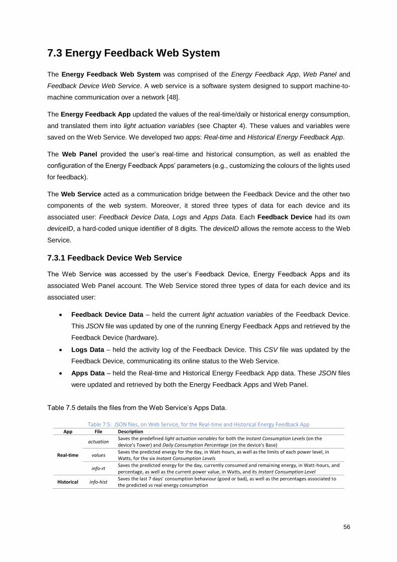
56
7.3 Energy Feedback Web System
The Energy Feedback Web System was comprised of the Energy Feedback App, Web Panel and
Feedback Device Web Service. A web service is a software system designed to support machine-to-
machine communication over a network [48].
The Energy Feedback App updated the values of the real-time/daily or historical energy consumption,
and translated them into light actuation variables (see Chapter 4). These values and variables were
saved on the Web Service. We developed two apps: Real-time and Historical Energy Feedback App.
The Web Panel provided the user’s real-time and historical consumption, as well as enabled the
configuration of the Energy Feedback Apps’ parameters (e.g., customizing the colours of the lights used
for feedback).
The Web Service acted as a communication bridge between the Feedback Device and the other two
components of the web system. Moreover, it stored three types of data for each device and its
associated user: Feedback Device Data, Logs and Apps Data. Each Feedback Device had its own
deviceID, a hard-coded unique identifier of 8 digits. The deviceID allows the remote access to the Web
Service.
7.3.1 Feedback Device Web Service
The Web Service was accessed by the user’s Feedback Device, Energy Feedback Apps and its
associated Web Panel account. The Web Service stored three types of data for each device and its
associated user:
• Feedback Device Data – held the current light actuation variables of the Feedback Device.
This JSON file was updated by one of the running Energy Feedback Apps and retrieved by the
Feedback Device (hardware).
• Logs Data – held the activity log of the Feedback Device. This CSV file was updated by the
Feedback Device, communicating its online status to the Web Service.
• Apps Data – held the Real-time and Historical Energy Feedback App data. These JSON files
were updated and retrieved by both the Energy Feedback Apps and Web Panel.
Table 7.5 details the files from the Web Service’s Apps Data.
Table 7.5: JSON files, on Web Service, for the Real-time and Historical Energy Feedback App App File Description
Real-time
actuation Saves the predefined light actuation variables for both the Instant Consumption Levels (on the device’s Tower) and Daily Consumption Percentage (on the device’s Base)
values Saves the predicted energy for the day, in Watt-hours, as well as the limits of each power level, in Watts, for the six Instant Consumption Levels
info-rt Saves the predicted energy for the day, currently consumed and remaining energy, in Watt-hours, and percentage, as well as the current power value, in Watts, and its Instant Consumption Level
Historical info-hist Saves the last 7 days’ consumption behaviour (good or bad), as well as the percentages associated to the predicted vs real energy consumption

57
7.3.2 Energy Feedback App
7.3.2.1 Real-time Energy Feedback App
The Real-time Energy Feedback App was a user-specific, always-on process executed at 20-second
intervals; it was responsible for computing the user’s Instant Consumption Level and Daily
Consumption Percentage, as well as translating them into corresponding Light Actuation Variables to
be used by the Feedback Device (see Chapter 4).
The Instant Consumption Level was the household’s real-time power consumption level. It had 6 levels
of consumption based on the computation of the last week’s power samples’ percentiles computed by
the Extractor. The Daily Consumption Percentage was the household’s energy consumption up to the
moment, expressed as a percentage of the predicted consumption for the day computed by the
Forecaster.
The app started by retrieving the Web Service’s files containing the information about the light actuation
variables’ default values (for the Daily and Instant Consumption), the predicted energy, as well as the
power levels’ values. After obtaining the user’s current energy consumption, the remaining and
consumed percentages are computed and sent to the Web Service (to be used by both Feedback
Device and Web Panel).
Using these percentages, the Base’s 22 LEDs were divided in two groups: the number of LEDs
associated with the remaining percentage was actuated in green; while the LEDs associated with the
consumed energy percentage were actuated in orange. The user may change the light actuation
variables’ default values through the Web Panel.
Afterwards, the household’s real-time power consumption was acquired, in Watts, and the current
Instant Consumption Level identified. This information was also sent to the Web Service, to be shown
on the Web Panel. The light actuation variables’ values for the levels can be changed through the Web
Panel. Table 7.6 shows the default values assigned for each level to be displayed in the EFD.
Table 7.6: Instant Consumption Levels – light actuation variables’ default values Very Low Low Medium Medium-High High Very High
Green & Static Green & Fade IO Orange & Static Orange & Fade IO Red & Static Red & Fade IO Legend: Fade IO – Fade In/Out
7.3.2.2 Historical Energy Feedback App
The Historical Energy Feedback App was an additional application, displayed on the Feedback Device
at 00:00 AM to show the user’s energy consumption behaviour over the last week. The app retrieved
the last 7 days’ predicted and consumed energy, computing the difference between these values for
each day, as well as the associated percentage of energy wasted (negative) or saved (positive). If the
day’s consumed energy was smaller than the predicted energy, it was considered a good day, otherwise,
it was considered a bad day. The days’ percentages, from the computed differences, were saved on the
Web Service (on the info-hist.json) and shown on the Web Panel.

58
As to the Feedback Device (hardware), the Base’s 22 LEDs were divided in 7 groups of 3 LEDs to
represent each day. The days were presented gradually on the device, from yesterday to the last 7th
day. If it was a good day, the 3-LEDs’ group associated to the day glows in green, otherwise in orange.
7.3.3 Web Panel
The Web Panel intended to provide further consumption information to the user, in both charts and
numerical format, as well as to allow the configuration of the available Energy Feedback Apps. Figure
7.3 presents a screenshot of the Home page of the Web Panel, for one of the users.
Figure 7.3: Web Panel Home Page for one of the participants
The first board displayed the Real-time Energy Feedback information, showing the current day’s values
of the Daily Consumption Percentage and Instant Consumption Level.
The second board displayed the Historical Energy Feedback information, showing the last week’s
consumption behaviour and associated percentage. The green days were the ones in which energy was
saved, while the red days were the ones in which energy was wasted. If the consumed energy surpassed
the predicted energy, it would be considered a bad day, otherwise it would be considered a good day.
We used an open-source responsive dashboard (https://adminlte.io), built on Bootstrap 3, as a starting
point for the development of the Web Panel. We designed the database using MySQLi and the
Login/Registration Form using PHP 7. Upon registration, the user must provide the deviceID associated
to his/her Feedback Device.

59
7.4 Conclusion
We developed a system architecture for the proposed cloud-based Energy Monitoring and Feedback
System. In terms of hardware, this system is comprised of a Wi-Fi electric meter’s sensor (as the
monitoring part) as well as of our Energy Feedback Device (as the feedback part). In addition, we
developed a software-based energy feedback solution, the Web Panel, which provides further
consumption information and allows the customization of the light colours and actions used in the EFD.
Furthermore, we have a cloud server (CentOS 6) as the core of the system, being responsible for
integrating both hardware and software components, run user-specific processes (in Python 2.7) and
save the users’ data.
The cloud server has three data systems. The Data Collection System updates the user’s current
power consumption as well as the temperature in the user’s geographical area, at 35-seconds intervals.
The Data Manager System, activated each day at midnight, computes the previous day’s variables
(i.e., electricity-related and temperature-related) and replaces invalid monitored days, due to the
sensor’s monitoring failures. The Data Forecasting System, activated each day at midnight, predicts
the day’s energy consumption (as the reference for the Daily Consumption Percentage) and computes
the references, i.e., power limits, for the Instant Consumption Level.
Moreover, another user-specific process is the Energy Feedback App, which acquires the user’s real-
time power consumption, to compute the current values for both Daily Consumption Percentage and
Instant Consumption Level. These values are then translated into their corresponding light actuation
variables and sent to the Feedback Device Web Service, which in turn acts as a communication bridge
between the Energy Feedback Device, the Energy Feedback App and the Web Panel.

60
Chapter 8: Experiment, Results and Evaluation
The developed Residential Energy Consumption Feedback Device (see Chapter 4) was installed in
some of the participants’ households (treatment group) to evaluate its effectiveness on feedbacking real-
time energy consumption. The goal was to change the occupants’ consumption behaviour into an
efficient one, that would ultimately lead to energy savings. The control group, without the device,
continued to be remotely monitored in order to evaluate their consumption during the same period.
In this chapter, we will present the design of the experiment, characterization of the households,
quantitative and qualitative analysis, and an overall evaluation of the results.
8.1 Design of the Experiment
An experiment intentionally imposes a treatment on a group of subjects to observe their response, as
approached [49]. The design of experiments (or quasi-experiments) refers to the design of any task that
intends to explain the variation of information, under conditions that are hypothesized to reflect the
variation [50].
We resorted to 6 participants’ households to conduct the experiments. As presented in Chapter 5, we
started by monitoring the energy consumption of 7 participants. However, one of the participants
abandoned the experiment due to major technical issues with his sensor.
In experiments, the subjects are usually divided into two groups: the treatment group – whereby the
treatments are applied to the group’s subjects; and the control group – a complementary group that
receives either no treatment or a standard treatment [49, 50].
On the treatment group, there are two types of variables: response variable (dependent) – focus of a
question in a study or experiment; and explanatory variable (independent) – which explains the
changes in the response variable [50, 51].
We had 5 Energy Feedback Devices available. Therefore, we randomly assigned 5 participants to the
treatment group and the remaining participant to the control group. In the treatment group’s households,
we installed our Energy Feedback Device (EFD). In the control group’s household, we continued to only
monitor its energy consumption.
The response variable was the household’s energy consumption, while the explanatory variable was
the installation of the EFD. The hypothesis was to test if the implementation of the EFD would bring a
reduction to the households’ energy consumption.
The Energy Feedback Devices were not delivered to the participants at the same time, being dependent
on the arrival and assembly of its casing and hardware components, and from the participant’s
availability to pick them up. Nevertheless, the devices were delivered between the last week of June
and first week of July. We also did not provide to the participants any information on energy efficient
actions, testing further the EFD effectiveness.

61
We will perform a quantitative analysis, using the methodology of a similar study [52], by comparing the
average energy consumption on the 30 days before vs. after the EFD implementation. We will also
resort to a paired T-Test to assess the statistical significance of the energy consumption for both periods.
Moreover, we will employ the Mean Percentage Error to compare the actual and predicted consumption
(by our forecasting algorithm) for both periods. These tests will also be applied to the control group, by
assigning a 30-day before and after period on the same time frame of the treatment group.
We will also perform a qualitative analysis, by survey: using Likert scales and open questions. This
analysis aimed to perceive the participant’s opinion on the EFD, mainly, assessing its informative ability,
aesthetics and impact on changing the consumption behaviour. The collected data, along with the
quantitative analysis, would provide an answer to the research question. Furthermore, we took
advantage of the survey to acquire more data, as regards to the occupant’s engagement, location of the
device, customer perspective and usage of the associated software on the cloud.
We aimed to reduce the Hawthorne effect, a type of reactivity on which subjects modify their behaviour
in response to their awareness of being observed [53], having no contact with the participants for almost
2 months, since the delivery of the device to the request of filling in the qualitative survey. Moreover, we
did not provide any information regarding energy efficient actions.
8.2 Participants households’ characterization
After the installation of the electric meter’s sensors, the participants filled in a survey related to their
household’s characterization (see Section 5.3.1). The survey was divided into two parts. The first part
aimed to gather information about the type of household, building, occupancy and electricity supply
contract. The second part, a multiple-choice survey, collected the appliances. The Households’ IDs from
1 to 5 belong to the treatment group while Household 6 belongs to the control group.
8.2.1 Characteristics of the participants’ household, building, occupancy and
electricity supply contract
Table 8.1 organizes the participants’ answers for the first part of the survey.
Table 8.1: Participants’ answers on their household type, building, occupancy and electricity supply contract
Categories Participant household (ID)
1 2 3 4 5 6 (Control)
Household Type Familiar Familiar Non-Familiar Familiar Familiar Familiar
N. of occupants 4 4 2 4 3 4
Building Type Apart. Apart. Apart. House Apart. Apart.
N. of rooms 4 3 3 6 3 4
Contracted Power (kVA) 6.9 6.9 3.45 6.9 6.9 6.9
Tariff Regime Bi-Hourly Bi-Hourly S. Tariff Bi-Hourly Bi-Hourly Bi-Hourly Legend: ID – Identifier; N. – Number; Apart. – Apartment; S. - Simple
As regards to the households, the number of occupants varied between 2 and 4, and the number of
rooms ranged from 3 to 6. All the participants lived in apartments, except one. Also, almost all the
participants lived with their families, having a contracted power of 6.9 kVA and a bi-hourly tariff, with the
exception of one participant (Household 3).

62
8.2.2 Appliances on the participants’ households
The second part of the survey details the type of appliances owned by each participant. Table 8.2
presents the results.
Table 8.2: Electrical Appliances on each one of the participants’ household and overall results
Category Appliance Participant household (ID) Results (overall)
1 2 3 4 5 6 N. households Percentage
Heating and Cooling Sources
Water Heater 3 50%
Elect. Heater 2 33%
Air Conditioning 2 33%
Fan Heater 2 33%
Oil-filled Heater 3 50%
Air Cooler Ventilator 0 0%
Fans 3 50%
Kitchen
Elect. Stove 2 33%
Induction Cooker 0 0%
Elect. Oven 3 50%
Elect. Fryer 0 0%
Elect. Grill 3 50%
Microwaves 6 100%
Elect. Kettle 5 83%
Coffee Machine 5 83%
Laundry and Food Coolers
Dishwasher 5 83%
Washer 6 100%
Dryer 3 50%
Fridge 0 0%
Fridge-Freezer 6 100%
Freezer 1 17%
Total number of Electric Appliances 12 10 6 7 12 11
Legend: ID – Identifier; N. – Number; Electr. – Electric.
The appliances common to all the participants are the microwaves, washer and fridge-freezer. Three of
the participants – two from the treatment and one from the control group – have a water heater,
responsible for the higher electricity consumption of these households.

63
8.3 Quantitative Results and Analysis
The quantitative analysis aims to assess the impact of the Energy Feedback Device (EFD) on the
household’s energy consumption.
As previously presented, we had a treatment group with the EFD installed in each participant’s
household, and a control group without the EFD. Within both groups, the participants’ energy
consumptions continued to be remotely monitored and collected.
To evaluate the EFD’s effectiveness in reducing the energy consumption, we resorted to the framework
employed on a previous study of the same kind [52], which divided the participants’ energy consumption
data in two periods:
• Before period: analysis of the participant’s household energy consumption, for a 30-day period,
before the installation of the EFD.
• After period: analysis of the participant’s household energy consumption, for a 30-day period,
after the installation of the EFD.
The devices were not delivered at the same time to all the treatment group’s participants, therefore, the
assigned periods have a difference of a few days across participants. Nevertheless, they were delivered
between the last week of June and the first week of July.
This methodology was also employed to the control group, by defining a 30-day before and after period,
over the same time frame as the treatment. This was done, of course, to compare both groups’ energy
consumption side-by-side.
With regards to the assignment of each one of the 30-day periods, we followed certain conditions. For
the treatment group, the starting date of the after period corresponded to the first time the EFD
communicated with our server, while for the control group, we assigned July as the after period.
Furthermore, invalid days (i.e., missing energy monitoring data due to sensor’s failure) were not
accounted for the analyses. Finally, the participants were instructed to turn off the EFD, if they left the
house without occupants for more than a day, therefore, on the after period, the days in which the EFD
was off were not accounted. Table A.8.1 (Annex 8) presents the dates of the before and after period
assigned to each participant.

64
8.3.1 Comparison of the daily average of energy consumption between periods
Considering the previously stated conditions, we collected the participant’s daily energy consumption
values, for a total of 60 days. To compare the energy consumption between participants, we
normalized the daily energy value, 𝑊(𝑛), of each one by using the following equation:
𝑊(𝑛)𝑛𝑜𝑟𝑚 =𝑊(𝑛) − 𝑚𝑖𝑛(𝑊)
𝑚𝑎𝑥(𝑊) − 𝑚𝑖𝑛(𝑊) (8.1)
In equation 8.1, 𝑊(𝑛) is the energy consumption for the day, 𝑛, in kWh; 𝑚𝑖𝑛 (𝑊) is the minimum
energy value, over the 60 days; and 𝑚𝑎𝑥 (𝑊) is the maximum.
Table A.8.2 (Annex 8) presents the minimum and maximum energy values for each participant, as well
as additional information of their energy data. Then, for each participant, we computed the average of
𝑊(𝑛)𝑛𝑜𝑟𝑚 for the 30 days before and after periods.
Figure 8.1 presents the results of this computation, depicting each participant’s normalized daily
average energy consumption over the 30-day before and after period.
Figure 8.1: Normalized daily energy consumption average – comparing the 30-day before vs. after period
Evaluating the results, we may conclude the treatment group’s households (1 to 5) reduced their daily
energy consumption, after the implementation of the Energy Feedback Device. Household 6 (control
group), without the Energy Feedback Device, showed an opposite behaviour increasing his daily energy
consumption on the after period.
Furthermore, to ease the understanding of these results, regarding each household’s energy
consumption difference between the before and after period, we employed the following equation:
∆𝑊%(𝑖) =𝑊𝑎𝑓𝑡𝑒𝑟(𝑖) − 𝑊𝑏𝑒𝑓𝑜𝑟𝑒(𝑖)
𝑊𝑏𝑒𝑓𝑜𝑟𝑒(𝑖)∗ 100 (8.2)
0,000000
0,100000
0,200000
0,300000
0,400000
0,500000
0,600000
0,700000
1 2 3 4 5 6
Dai
ly A
vera
ge (n
orm
aliz
ed)
House
Daily Energy Consumption Average
before
after

65
In equation 8.2, 𝑊𝑎𝑓𝑡𝑒𝑟(𝑖) is the daily average of energy consumption of household 𝑖 over the 30-day
after period; and 𝑊𝑏𝑒𝑓𝑜𝑟𝑒(𝑖) is the daily average of energy consumption of household 𝑖 over the 30-day
before period, in kWh. Table 8.3 presents these values for each household as well as the results in
percentage, by applying equation 8.2.
Table 8.3: Before and after energy consumption – daily average – in kWh and percentage Treatment Control
𝒊 𝑯𝒐𝒖𝒔𝒆𝒉𝒐𝒍𝒅 𝟏 𝑯𝒐𝒖𝒔𝒆𝒉𝒐𝒍𝒅 𝟐 𝑯𝒐𝒖𝒔𝒆𝒉𝒐𝒍𝒅 𝟑 𝑯𝒐𝒖𝒔𝒆𝒉𝒐𝒍𝒅 𝟒 𝑯𝒐𝒖𝒔𝒆𝒉𝒐𝒍𝒅 𝟓 𝑯𝒐𝒖𝒔𝒆𝒉𝒐𝒍𝒅 𝟔
𝑾𝒃𝒆𝒇𝒐𝒓𝒆(𝒊) 19.75 10.39 4.12 8.82 12.75 11.46
𝑾𝒂𝒇𝒕𝒆𝒓(𝒊) 16.60 8.79 2.96 6.43 8.15 11.68
∆𝑾%(𝒊) -16% -15% -28% -27% -36% +2%
The least decrease in energy consumption occurred in Household 2 (15%), followed by Household 1
(16%), Household 4 (27%), and Household 3 (28%). The EFD was most effective in Household 5, with
a remarkable decrease of energy consumption by 36%.
After the implementation of the Energy Feedback Device, we can ultimately conclude that the treatment
group’s participants reduced their daily average consumption by 15% to 36%. On the other hand, the
control group participant increased his consumption by 2%. Figure 8.2 illustrates the results of the
energy savings for the treatment group.
Figure 8.2: Energy savings of the treatment group (compared to the 30 days previous to the EFD implementation)
As mentioned earlier, Household 5 was the participant with the largest reduction (36%). As claimed by
this participant on the qualitative analysis (Section 8.4), he understood, through the EFD, the excessive
energy usage of his water heater. Therefore, he reprogrammed the operation of this energy-hungry
appliance and he adopted, along with his family, an efficient consumption behaviour by following the
EFD indications.
These results provide us positive results towards energy savings upon the implementation of the EFD.
On the next section, we will perform a statistical test to check the significance of data.
16% 15%
28% 27%
36%
0%
5%
10%
15%
20%
25%
30%
35%
40%
Household 1 Household 2 Household 3 Household 4 Household 5
Energy savings of the treatment group

66
8.3.2 Statistical test
We employed statistical hypothesis tests, a method of statistical inference used to determine what
outcomes of a study would lead to the rejection of the null hypothesis for a pre-specified level of
significance [54]. We employed a paired T-test, comparing the before and after period’s energy average,
by defining two hypotheses:
1) Null Hypothesis: There is no effect on the energy consumption values, even if the Energy
Feedback Device has been installed on the household. Therefore, the before and after period’s
energy average are the same and the device is not effective.
2) Alternative Hypothesis: There is a significant difference in the energy average between the
two periods, being significantly lower with the Energy Feedback Device than without it.
Rule for rejecting the Null Hypothesis: If the p-value is smaller than 0.05 (95% of confidence level
over the results) the difference is significant, otherwise, the null hypothesis is to be accepted.
Table 8.4 presents the computed p-value, for the treatment and control group, considering the before
vs. after 30-days period.
Table 8.4: p-value results of the Paired T-Test Treatment Control Household 1 Household 2 Household 3 Household 4 Household 5 Household 6
p-value 0.009255 0.025789 2.56E-06 5.02704E-05 1.34E-06 0.277466
All the treatment group participants had a p-value lower than 0.05, therefore, we can reject the null
hypothesis and conclude that the daily average consumption with the EFD is significantly smaller than
without it (with 95% of confidence level).
In other words, we can conclude that our EFD saved energy. The results compel us to recommend its
implementation to reduce electricity costs.
On the other hand, Household 6 (control group), without the EFD, had a p-value higher than 0.05.
Therefore, we can accept the null hypothesis, showing that the daily average consumption remained
the same.

67
8.3.3 Mean percentage error
We performed a final verification of the quantitative results through the Mean Percentage Error – by
comparing the actual and predicted consumption of the participants for both before and after period.
To do so, we applied our forecasting algorithm (see Chapter 6) to obtain the predicted consumption for
each day to then compare it with the actual consumption.
The Mean Percentage Error (MPE) is the average of percentage errors by which the predicted values
differ from the actual values. We applied the following equation to compute the MPE:
𝑀𝑃𝐸 =100%
𝑛∑
𝑊𝑖 − 𝑊𝑒𝑠𝑡𝑖
𝑊𝑖
𝑛
𝑖=1
(8.3)
In equation 8.3, 𝑊𝑖 is the actual energy consumption, 𝑊𝑒𝑠𝑡𝑖 is the predicted consumption for the day,
and 𝑛 is the total number of days. We applied equation 8.3 for both the 30-day after and before period.
Table 8.5 presents the results of the MPE of each participant for both periods.
Table 8.5: Mean Percentage Error results (before and after period) Household Before After
1 1% -20%
2 -9% -15%
3 3% -25%
4 -1% -25%
5 -1% -35%
6 (control) -2% 3%
In the before period, the MPE between the real and predicted energy consumption is in the range of -
3% to 3%, except for Household 2 with -9%.
In the after period, the treatment group’s MPE is in the range of -15% to -35%; while the control group’s
participant – without the device – has a value of 3%.
Therefore, using this method, we can verify that during the before period the MPE has a small value for
all the participants.
Upon the installation of our Energy Feedback Device – associated to the after period – we can verify a
significant difference between the predicted and actual energy of the treatment group’s participants, and
more importantly, a negative difference – meaning that the treatment group is consuming less than
predicted. On the other hand, the control group participant remains with a small MPE value.

68
8.4 Qualitative Results and Analysis
We concluded, on the quantitative analysis, that our EFD brought energy savings. Using this survey, we
want to correlate these discoveries with the user’s opinion on its ability to inform and consequentially
change user behaviour. Besides that, other information was collected as to the device aesthetics, user’s
engagement, buyer perspective and the use of the Web Panel.
The survey sent to the treatment group’s participants (available on http://bit.ly/2xUdant) was created to
understand the following topics:
1) Device’s placement, occupants’ engagement and motivation for its usage.
2) Presentation of consumption information, device’s aesthetics and its impact on modifying the
user’s consumption behaviour.
3) Customer’s perspective over the system (their preferred model for our revenue streams)
4) Web Panel (cloud-based software platform) and NFC Tag
8.4.1 Placement, occupant’s engagement and motivation
Table 8.6 summarizes the questions and answers for this topic.
Table 8.6: Placement, location, occupant’s engagement and motivation answers
Questions / Categories Answers and percentage
Placement
Location of the device (household’s room) Living Room (100%)
Device degree of visibility on the room Very visible (100%)
Location and occupant’s engagement Yes No
Most common room of the house 100% 0%
Device integrated aesthetically on the room 80% 20%
Occupants understand the device 100% 0%
Occupants react to the device 100% 0%
Interaction with the device 1 to 5 per day 6 to 10 per day
Number of times, on average, the device is checked 20% 80%
Motivation for the device’s usage Reduce the cost of the electricity bill Reduce environmental impact
Most important motivation to use the feedback device 60% 40%
Upon the delivery of the EFD, we instructed the participants to place it in the most “social” compartment
of their household and try to engage their family with the device. These requests were fulfilled, as shown
in Table 8.6, for both ‘placement’ and ‘location and occupant’s engagement’ categories.
Most of the participants checked the device from 6 to 10 times a day. Their main motivation for the
device’s usage was to reduce the cost of the electricity bill, although 40% claimed that their most
important motivation was to reduce their environmental impact.

69
8.4.2 Consumption feedback, aesthetics and impact on behaviour
We employed a Likert five-point scale (very poor, poor, fair, good and very good) to rate the following
topics. Table 8.7 summarizes the answers given by the treatment group’s participants.
Table 8.7: Device ratings over aesthetics, real-time and daily consumption feedback and impact on behaviour modification Categories and questions/parameters Answers – scale’s categories (percentage)
Very Poor Poor Fair Good Very Good
Device’s rating (overall)
Aesthetically pleasing 0% 0% 20% 40% 40%
Ability to inform about real-time and daily consumption 0% 0% 0% 0% 100%
Impact on modifying the consumption behaviour 0% 0% 0% 40% 60%
Real-time consumption feedback
Ease of understanding 0% 0% 0% 20% 80%
Predefined light’s colours and actions for the levels 0% 0% 0% 60% 40%
Aesthetics 0% 0% 0% 40% 60%
Daily consumption feedback
Ease of understanding 0% 0% 0% 20% 80%
Predefined light’s colours for the percentages 0% 0% 0% 60% 40%
Aesthetics 0% 0% 0% 40% 60%
All the participants gave the best rating to the device’s ability to inform about the real-time and daily
consumption and 60% gave the best rating to its impact on modifying their consumption behaviour, while
the remaining classified it as ‘good’. The ‘aesthetically pleasing’ was the only topic that received a ‘fair’
grade by one of the participants, while the rest considered it either ‘good’ or ‘very good’. It should be
noticed that the prototype was 3D-printed, which gives room for later improvements on its aesthetics.
For both real-time and daily consumption feedback, the vast majority of the participants (80%) gave the
best rating to the ease of understanding the information. The predefined light’s colours and/or actions
were considered ‘good’ for 60% of the respondents, while the feedback light’s aesthetics were
considered ‘very good’ by 60%.
With regards to additional comments: “Device was quickly accepted by my family and influenced the
reduction over the energy consumption”, “The device greatly altered my perception of energy
consumption. Now, I turn off the TV during the night and close the lights on rooms that I’m not currently
in. I use less often the electric kettle less often and when I do, I lay a lesser amount of water. I modified
the temperature of the fridge and identified a problem of ice accumulation on the fridge’s freezer,
consuming more energy, as its door was not closing correctly. These habits have reduced my
consumption, as I live in a small house”, “I understood the excess of energy consumption from my water
heater, due to the real-time energy consumption feedback and I’ve reprogrammed its operation”.
As regards to improvements: “the transparency of the device makes the light very intense at night”, “the
device should turn off automatically in times where there is no one at home, or even at night. I mean,
when there is no electricity consumption or if it is very low, below a certain level”.

70
8.4.3 Customer’s perspective
In this topic, we aimed to collect the participants’ opinion as customers. We provided three possible
models for the acquisition of the overall system (i.e., electric meter’s sensor and Energy Feedback
Device): buy, rent by paying an annuity or rent by paying a monthly fee.
Most of the respondents preferred to rent the system during a year (60%), while no participant preferred
to rent the system by paying a monthly fee. The remaining participants (40%) preferred to buy the
system.
The evaluated price for the annuity was between 50€ and 80€. More specifically, considering the
multiple-choice ranges available, the results were: 50-60€ (40%), 61-70€ (20%) and 71-80€ (40%).
As regards to buying the system, the evaluated price was between 125€ and 200€. The multiple-choice
ranges chosen were: 125-150€ (40%), 151-175€ (40%) and 176-200€ (20%).
One of the participants answered the optional open question, to provide additional comments: “In terms
of a possible purchase (buy), I consider that the asked value should never be superior to the value of
the energy savings over a year. If that was the case, I would have all the interest in buying one or more,
to place them on different rooms of my house”.
8.4.4 Web Panel and NFC Tag
The Web Panel was the software-based feedback solution (on www.beaware.club), providing access to
further energy consumption information and allowing the customization of the Energy Feedback
Device’s colours and actions employed for consumption feedback.
All the participants accessed to the Web Panel. The main motive was to check their electricity
consumption information – real-time, daily and historical (i.e., last week). On the other hand, 60% of the
respondents used it to run the historical consumption app and other 60% used it to customize the colours
used in the device.
The NFC Tag was a way to quickly access to the Web Panel, by approaching a smartphone or tablet
with this technology to the Energy Feedback Device. However, 60% of the participants did not use it,
because their equipment did not support this technology. We learnt that iPhone does not use this
technology the same way as Android smartphones do, being this the main reason for its lack of use.
As regards to additional comments and suggestions for improvement: “The Web Panel was very
versatile. On the historical consumption, the time frame should be increased. However, I’ve used it
several times per week, inside and outside my house, to check the consumption.”; “The Web Panel
should have a set of themes with predefined colours for the device, so the user could easily experiment
other combinations without having to write the RGB values one by one”

71
8.5 Conclusion
We developed an intuitive “tool”, so that consumers can understand and act upon their current
consumption behaviour. However, our device is directed to educated and conscious consumers, who
understand the problems of the excessive use of resources in our planet, and do their part to counteract
it.
The purpose was to create an Energy Feedback Device that was informative, aesthetically pleasing and
perceivable by everyone. More importantly, it aimed to feedback energy consumption in a way that
would lead to a change of householder’s consumption behaviour into an efficient one, ultimately leading
to energy savings.
Upon literature review, previous studies showed that the use of energy feedback devices (or in-home
displays) can provide energy savings between 5% and 15% [22]. Most of these devices present the
units of energy consumption on LCDs.
Our new approach on feedbacking energy consumption through the developed Residential Energy
Consumption Feedback Device, brought energy savings between 15% and 36% as presented in the
qualitative analysis of the treatment group, by using a methodology similar to the one employed in a
previous study [52]. On the other hand, the participant in the control group, without the device, increased
his energy consumption by 2%.
As an example, Household 5 understood through the device, that his water heater was consuming more
energy than needed. Therefore, he reprogrammed it, as well as employed an efficient consumption
behaviour (by following the feedback of our device), reaching to 36% of energy savings when compared
to the period without the device.
We also performed a confirmatory data analysis of the treatment group’s energy data, using a paired T-
test. The test confirmed the device’s impact, showing a significant difference in the daily average of
energy consumption, between the period with and without our Energy Feedback Device. The p-value of
the best result was 1.34E-06 and the worst was 0.025789, presenting a confidence level higher than
95%. We had a small number of participants, due to the limited number of devices, but this may
constitute a starting point for the understanding of energy feedback devices’ intuitive design.
We performed a final verification of the quantitative results through the Mean Percentage Error (MPE),
by comparing the participant’s real and predicted consumption for both before and after period. In the
before period, the MPE was between -2% to 3% (except for Household 2 with -9%). In the after period,
the treatment group’s participants MPE was between -15% to -35%, showing that they were consuming
less than predicted. On the other hand, the control group’s MPE for the after period was 3%.
To confirm the quantitative results, we performed a qualitative analysis of the participant’s opinion on
the device. All the participants placed their EFD in the most visible place of their living room, claiming
that all the other occupants understood and interacted with the device, thereby contributing towards an
efficient consumption for the household.

72
Most of the participants checked the device, on average, 6 to 10 times per day (80%). The most
important motivation for its use was the reduction of the electricity bill (60%), while the remaining claimed
that reducing their environmental impact was the main motivation for the device’s usage.
All the participants gave the best rating to the device’s ability to inform about the real-time and daily
consumption, and most (80%) gave the best rating for the ease of understanding its information. Most
of the participants (60%) gave the best rating to the EFD’s impact on modifying their consumption
behaviour, while the remaining classified it as ‘good’. Also, 60% of the participants rated the light’s
aesthetics on transmitting information as ‘very good’ (best rating). One of the participants gave a ‘fair’
rating to the ‘aesthetically pleasing’ topic, while the rest considered it either ‘good’ or ‘very good’. Finally,
most of the respondents (60%) considered the predefined colours for presenting the real-time and daily
consumption as ‘good’, while the remaining gave the best rating to it.
From a customer’s perspective, most of the respondents preferred to rent the system by paying an
annuity (60%) while the others preferred to buy it. No one preferred to rent it by paying a monthly fee.
The evaluated price for the annuity was between 50€ and 80€, while the values for the purchase of the
system varied between 125€ and 200€.
The Web Panel (www.beaware.club) was accessed by all of the participants. All of them used it to
access the electricity consumption information while 60% used it either to customize the lights’ colours
of the device or to run the historical consumption app.
The NFC Tag, placed at the front side of the device, aimed to provide a quick access to the Web Panel,
by approaching an NFC-enabled device (smartphone or tablet) to the tag. Most of the participants did
not use it (60%), as their equipment do not support this technology.
In terms of improvement suggestions, the participants claimed that the energy values of historical
consumption should be presented at larger intervals of time. In terms of customizing the colours of the
device, we should provide several themes of colours besides the predefined traffic lights scheme.
In terms of the device itself, the transparency of the device’s 3D-printed mock-up makes the light very
bright and the intensity of the light should be adapted (through Web Panel). Also, participants suggested
that the device could turn off its lights if there was no one at home, or even at night.
Finally, with regards to the research question, based on the collected data from the experiment, we can
answer affirmatively. The device was shown to be informative and aesthetically pleasing, changing the
participants’ behaviour towards an efficient one, and resulting in energy savings superior to the ones
found in previous studies – 4%-15% and 5%-15% [21, 22].

73
Chapter 9: Conclusions and Future Work
This work is in the scope of Energy Monitoring and Feedback Systems (EMFS) for residential
consumers, focusing on the design and test of an Energy Feedback Device (EFD) with differentiating
features when compared to the ones found in most commercial products. The main objective of this
work can be reflected by the following research question: Can an Energy Feedback Device bring energy
savings and be simultaneously pleasant and informative to the consumer?
The objective was to develop a device that encourages electricity consumers to enhance their energy
efficiency, by resorting to innovative ways of presenting their current consumption behaviour. The EFD
aimed to be informative, intuitive and aesthetically pleasing; with the goal of bringing energy savings by
influencing the modification of the residential consumers’ behaviour.
9.1 Summary
This thesis starts with an introductory chapter presenting the research background, research question
and its contributions, and ends with Chapter 9, where the conclusions of this work are presented.
In Chapter 2 we started by reviewing the literature related to the impact of occupants’ behaviour over
energy consumption. Moreover, we reviewed studies on the Energy Feedback Devices’ potential over
energy savings as well as their current problems.
In Chapter 3 we performed a brief market research, whereby we surveyed 47 providers of Energy
Monitoring and Feedback Systems and analysed the features of 20 commercially available Energy
Feedback Devices. Moreover, we hypothesized and interviewed potential customers for such devices.
In Chapter 4 we proposed an Energy Feedback Device with differentiating features, based on the
previously collected data, as well as presented its components, i.e., casing, hardware and firmware.
In Chapter 5 we gathered residential energy consumers as the participants of our experiments, through
a campaign. In this first stage of the experiment, we installed Wi-Fi electric meter’s sensors on the
participants’ households, to have remote access to their energy consumption. We also performed the
households’ characterization, through a survey, and based on our proposed framework.
In Chapter 6 we presented the process used for the development of the energy forecasting algorithm,
to find a method and its associated parameters, for the prediction of the following day’s energy
consumption of a household.
In Chapter 7 we proposed a system architecture for our cloud-based Energy Monitoring and Feedback
System, constituted by the cloud server and its hardware and software components.
In Chapter 8 we presented the second stage of the experiment, in which we installed our Energy
Feedback Device in the treatment group’s households to answer to the research question. Moreover,
we assessed the impact of our EFD on the participants’ energy consumption by conducting both a
quantitative and qualitative analysis.

74
9.2 Conclusions
In the literature review, we found that one of the best ways to modify occupants’ consumption behaviour
into an efficient one is by providing frequent feedback of their consumption [16]. According to [22] the
best way to visualize the household’s real-time energy consumption information is by using an Energy
Feedback Device (also known as In-Home Display) which in turn can bring energy savings ranging from
5% to 15%. However, most of these devices are considered unintuitive, as some householders cannot
understand the displayed information, thus, there is a need to make them user-friendly [6,20].
According to [23], the EFDs can be classified into 3 types, depending on the way they present energy
consumption information: numerical display (using numbers), analogue display (using scales) and
ambient display (using alternative ways to numbers and scales, e.g., light, sound, movement, etc.) [23].
We found a scarcity of literature over the design and test of ambient EFDs. However, Chiang’s study [6]
showed the potential of ambient displays on energy savings, when compared with the other two types.
In the market analysis, we found that most of the EMFS’ providers present solutions for commercial
(83%) and/or industrial clients (77%). The residential consumers were disregarded as only 45% of the
companies targeted them. Moreover, we found that most companies provide software-based feedback,
whereby consumption information is displayed through software platforms (i.e., mobile app, desktop
and/or web); as opposed to hardware-based feedback, whereby information is displayed through EFDs.
We approached three customer segments: small and medium businesses, hospitality landlords and
residential consumers. The first two preferred to have an EFD on their homes, where they can control
energy consumption. We chose residential consumers as our main customer segment. We found that
most of them (80%) felt lack of control over energy consumption, showing interest in the acquisition of
system that would help them to save energy. Moreover, 70% of the respondents preferred an intuitive
(i.e., avoiding “technical details”) hardware-based solution, rather than a software-based solution.
We found that most of the 20 commercially available EFDs targeted are featured by: an LCD (90%)
presenting consumption information through numerical (50%) or analogue displays (40%), i.e., through
numbers or scales, and using Radio Frequency (95%), instead of Wi-Fi, to communicate with a
company-specific sensor. Therefore, we proposed the following differentiating features for our
standalone EFD: a device that uses light to present the consumption behaviour through colour-coded
information, using Wi-Fi to connect to a cloud server, which in turn communicates with a third-party Wi-
Fi electric meter’s sensor.
We proposed two colour-coded information (which reference values are updated each new day) and
associated to the instant (power-related) and daily (energy-related) consumption. The Instant
Consumption Level is the household’s real-time power consumption presented in 6 colour-coded levels:
very low, low, medium, medium-high, high and very high. These levels were distinguished by both their
colour and light’s action. We colour-coded the levels using the universally known traffic light’s scheme
(i.e., low levels in green, medium levels in orange and high levels in red). We used light actions to
distinguish between levels with the same colour, whereby the first is a static light (no action) and the

75
second a fade in/out light, e.g., the medium level is an orange static light and the medium-high level is
an orange light fading in and out. The Daily Consumption Percentage is the household’s energy
consumption up to the moment, presented as a percentage of the predicted energy for the day. This
required the development of an energy forecasting algorithm, presented in Chapter 6, to predict the
following day’s energy consumption. For this consumption information we used a light-coloured circle to
represent the percentage of both remaining and consumed energy related to the predicted energy for
the day (in a green and orange static light, respectively).
To design an ambient EFD that uses colour-coded light to feedback consumption information, we
resorted to Prof. Paulo Parra and his team (Faculdade de Belas-Artes da Universidade de Lisboa). We
worked together on all the development stages of the EFD, to make it both user-friendly and aesthetically
pleasing, resulting in a 3D-printed final prototype. Moreover, we developed a Printed Circuit Board to be
implemented in the prototype, with the objective of connecting the EFD to the cloud and to perform the
light actuation, through its LEDs, of the colour-coded current consumption information.
We created a campaign and collected 7 residential energy consumers, as the participants of our
experiments. We found that Portuguese online communities related to energy efficiency, environment
and renewable energies are almost inexistent or inactive, therefore, they are not suitable for the
acquisition of participants. On the other hand, we found that technology enthusiasts are easier to find
and willing to enrol as participants. In this first part of the experiment, we installed Wi-Fi electric meter’s
sensors on their households to remotely monitor their energy consumption. Moreover, we conducted a
survey to characterize the participants’ households, based on our proposed framework.
We developed a forecasting algorithm to predict the following day’s energy consumption of a household.
We targeted two methods: Linear Prediction and Decision Trees (Regression Tree, Random Forests
and Extremely Randomized Trees). We experimented different conditions (e.g., training period, input
variables, etc.) for the tests, to choose the method and its associated parameters presenting the best
results for our data, evaluated by the mean absolute error. We resorted to a year of energy consumption
data from a family of four, dividing it into a training, validation and test set. The vast majority of the tests
and the final algorithm resorted to Python 2.7 and scikit-learn (a free machine learning library).
We started with Linear Prediction by testing two hypotheses. The first (Hypothesis I) used a simple
average while the second (Hypothesis II) used a weighted average by computing the predictor
coefficients. In our data, the best method was found for Hypothesis I, when predicting a day’s energy
consumption based on the average consumption of the last 7 days. Its mean absolute error was
employed as a baseline, when experimenting the Decision Trees’ methods.
On the Decision Trees’ methods, we found that Extremely Randomized Trees presented a smaller mean
absolute error when compared under the same conditions to Regression Tree and Random Forests.
Moreover, the use of 28 previous days as the training period (i.e., 4 weeks) presented a smaller mean
absolute error when compared to the other experimented periods (in multiples of 7, i.e., weeks, e.g., 7,
14, 21, 35, etc.). As to the pre-pruning parameters, to avoid overfitting and underfitting, the best case
was found when limiting a maximum of 4 leaf nodes combined with a minimum of 5 required samples

76
to define a leaf node as well as using the mean absolute error to evaluate the quality of a split. Finally,
we tested the number and type of input variables, using greedy algorithm to find the locally optimum
solution (due to the large number of possible combinations) and mean absolute error – concluding that,
in our data, the best results were found for the following 11 input variables: 𝑃𝑚𝑒𝑑7(𝑛), 𝑃𝑚𝑒𝑑(𝑛 − 1),
𝑊14(𝑛), 𝐷𝑎𝑦(𝑛), 𝐶𝐷𝐷(𝑛 − 1), 𝑇𝑚𝑒𝑑(𝑛 − 1), 𝑊(𝑛 − 1), 𝑃𝑚𝑎𝑥7(𝑛), 𝑊28(𝑛), 𝑇𝑚𝑖𝑛7(𝑛) and 𝑊7(𝑛) (Table
A.6.4 in Annex 6 describes them). We chose Extremely Randomized Trees with a total of 10 trees using
the previously presented parameters, due to its better performance prediction.
We developed a system architecture for the proposed cloud-based Energy Monitoring and Feedback
System. In terms of hardware, this system is comprised of a Wi-Fi electric meter’s sensor (as the
monitoring part) as well as of our Energy Feedback Device (as the feedback part). In addition, we
developed a software-based energy feedback solution, the Web Panel, which provides further
consumption information and allows the customization of the light colours and actions used in the EFD.
Furthermore, we have a cloud server (CentOS 6) as the core of the system, being responsible for
integrating both hardware and software components, run user-specific processes (in Python 2.7) and
save the users’ data.
The cloud server has three data systems. The Data Collection System updates the user’s current
power consumption as well as the temperature in the user’s geographical area, at 35-seconds intervals.
The Data Manager System, activated each day at midnight, computes the previous day’s variables
(i.e., electricity-related and temperature-related) and replaces invalid monitored days, due to the
sensor’s monitoring failures. The Data Forecasting System, activated each day at midnight, predicts
the day’s energy consumption (as the reference for the Daily Consumption Percentage) and computes
the references, i.e., power limits, for the Instant Consumption Level.
Moreover, another user-specific process is the Energy Feedback App, which acquires the user’s real-
time power consumption, to compute the current values for both Daily Consumption Percentage and
Instant Consumption Level. These values are then translated into their corresponding light actuation
variables and sent to the Feedback Device Web Service, which in turn acts as a communication bridge
between the Energy Feedback Device, the Energy Feedback App and the Web Panel.
After the development of the device and its system architecture (i.e., EMFS), we needed to test the
EFD’s effectiveness in order to answer to the research question. In the first phase of the experiment,
we started by monitoring 7 participants, however, one of them had major technical issues with his
sensor, ending up abandoning the experiment. Therefore, we had a total of 6 participants. In the second
phase of the experiment, we installed the EFD in the households of the treatment group’s participants.
Due to the limited number of available EFDs, we randomly chose 5 participants for the treatment group,
while the remaining participant was assigned to the control group.
In the quantitative analysis, we used a methodology similar to [52], by dividing the treatment group
participant’s daily energy consumption data into two periods of 30 days: one before the installation of
the EFD and another after. We also defined two 30-day periods for the control group (without the EFD),
using a time frame similar to the treatment group. Then, we compared the average energy consumption

77
for both before and after period, whereby the treatment group’s participants reduced their energy
consumption between 15% and 36%. The results were statistical significant, when applying a paired t-
test (confidence level of 95%). In opposition, the control group increased the consumption by 2% and
showed no statistical significance when comparing both periods. We also applied the Mean Percentage
Error (MPE) to compare the participant’s real and predicted consumption for both periods. In the before
period, the MPE was between -2% and 3% (except for Household 2 with -9%). In the after period, the
treatment group’s MPE was between -15% and -35%, showing that they were consuming less energy
than predicted. Contrarily, the control group’s MPE was 3%, showing no significant difference.
In the qualitative analysis, we surveyed the treatment group’s participants mainly using a 5-point Likert
Scale (very poor, poor, fair, good and very good). All the participants gave the best rating for the device’s
ability to inform about the real-time and daily consumption, and most (80%) gave the best rating for the
ease of understanding the consumption information. Moreover, most (60%) of the respondents gave the
best rating to the EFD’s impact on modifying their consumption behaviour, while the rest classified it as
‘good’. As to the overall aesthetically pleasing aspect of the device (i.e., 3D-printed prototype), the
participants classified it either ‘very good’ (40%) or ‘good’ (40%), except for a participant that classified
it as ‘fair’. All participants placed the device in their living room and all the occupants interacted with it,
thereby contributing for the household’s efficient consumption. From the customer’s perspective, 60%
of the participants preferred to rent the system by paying an annual fee (between 50-80€) while the rest
preferred to buy it (between 125-200€). All the participants accessed the Web Panel (software-based
feedback platform), and only 40% used the NFC Tag, to quickly access to the Web Panel, by
approaching a smartphone or tablet with this technology to the device (most of them, 60%, did not use
it as the iPhone cannot use this technology the same way as Android Smartphones do).
9.3 Final overview
This work presented a process that can be generalized for the development and test of other cloud-
based technology products, when focused in the discovery and implementation of innovative features.
In our case, we targeted EFDs (and consequently EMFS). We started by reviewing the existing literature,
to understand their potential over energy savings as well as their current problems. Then, we performed
a market analysis (to the currently available products) to confirm some of the literature review’s findings
and to identify differentiating features for our EFD. We also hypothesized customer segments and
interviewed potential clients, to identify the most suitable and to collect their opinions over EFDs.
We found that most of the commercially available EFDs have the following features: an LCD presenting
consumption information through numbers or scales and using Radio Frequency to communicate with
a specific sensor. We defined the following differentiating features: a device that uses light to present
the consumption behaviour (real-time and daily) through colour-coded information, resorting to Wi-Fi to
communicate with a cloud server, which in turn communicates with a third-party Wi-Fi electric meter’s
sensor.
Since an EFD is constantly interacting with the consumer, the device must be to be informative, intuitive,
user-friendly and aesthetically pleasing. Therefore, to enhance the quality of human-machine

78
interaction, we resorted to two knowledge areas – design and engineering. As a cloud-based product,
we also developed a system architecture (related to the overall EMFS), comprised of the cloud server,
as the core of the system, as well as of the system’s hardware and software components.
After developing both EFD and EMFS, we tested the effectiveness of our solution. Therefore, we
acquired participants (residential consumers) through a campaign. We started by installing the third-
party electric meter’s sensor on the participants’ households to remotely monitor their energy
consumption, prior to the implementation of the EFD. Then, we implemented our EFD, which brought
energy savings (15%-36%) superior to the ones found in the literature review from (5%-15% [22]),
through the modification of the householders’ consumption behaviour. Moreover, according to the
surveyed participants, our EFD prototype fulfilled the proposed objectives, as by their overall opinion it
was considered intuitive, easy to understand and aesthetically pleasing.
9.4 Future Work
The proposed EFD encompasses several areas. Therefore, we will present the following topics as the
most important ones to be approached in a future work.
Firstly, using a larger and equal number of subjects for both treatment and control groups would increase
the scope of the experiment. Furthermore, another quantitative analysis could be conducted using a
larger period of consumption data.
Secondly, further work can be done on the proposed forecasting algorithm to increase its accuracy
towards energy consumption prediction, which in turn is used as a reference for the Daily Consumption
Percentage, i.e., the consumed and remaining energy percentage based on the predicted consumption
for the day. Also, other methods can be tested for the definition of the power intervals for the six levels
of the Instant Consumption Level, i.e., the household’s current power consumption represented in levels.
Thirdly, as to the presentation of these two consumption-related information, we suggest the test of
alternative approaches, such as using other predefined light actions and colours (besides the traffic light
scheme), including a “sleep” function (i.e., turning of the device’s lights when the consumption is too
low, or when no one is home) and automatically adjusting the light intensity (day vs. night).
Fourthly, as to the Energy Feedback Device, we may consider the use of other materials to improve its
aesthetically pleasing aspect, such as the use of epoxy instead of 3D-printed material. As to the
Feedback Device’s Tower, other forms could also be tested.
Fifthly, the Web Panel may be improved. We suggest the presentation of the historical consumption
using larger periods, provide several predefined themes for the customization of the light’s colours and
actions used for feedback, and allow the adjustability of the device’s light intensity.
Lastly, other methods could be tested to replace the invalid monitored days due to the sensor’s failures.
Moreover, other customer segments could be approached, e.g., co-working and open space offices.
Despite the need of further work, the proposed EFD showed satisfactory results towards energy savings
for residential consumers.

79
References
[1] Direcção-Geral de Energia e Geologia (DGEG), “Energia em Portugal,” 2014.
[2] Eurostat, “Greenhouse gas emissions by industries and households,” 2016. [Online]. Available:
http://ec.europa.eu/eurostat/statistics-
explained/index.php/Greenhouse_gas_emissions_by_industries_and_households#Analysis_by_econ
omic_activity
[3] S. Sorrell, “Reducing energy demand: A review of issues, challenges and approaches,” Renew.
Sustain. Energy Rev., vol. 47, pp. 74–82, 2015.
[4] Y. T. Chen, “The factors affecting electricity consumption and the consumption characteristics in the
residential sector — a case example of Taiwan,” Sustain., vol. 9, no. 8, 2017.
[5] I. Laicane, A. Blumberga, M. Roša, and D. Blumberga, “Determinants of household electricity
consumption savings: A Latvian case study,” Agron. Res., vol. 12, no. 2, pp. 527–542, 2014.
[6] T. Chiang, “Investigating the influence of in-home display design on energy-consumption behavior,”
Ph.D. dissertation, Dept. of Architecture and Civil Eng., Bath Univ., UK, 2015.
[7] A. Summerfield, T. Oreszczyn, A. Pathan and S. H. Hong, “Occupant behaviour and energy use,” in
A handbook of sustainable building design and engineering: an integrated approach to energy, health
and operational performance, D. Mumovic and M. Santamouris, Eds. London: Taylor & Francis, 2009,
pp. 359-370.
[8] F. Van Raaij and T. Verhallen, “A behavior model of residential energy use,” Journal of Economic
Psychology, vol. 3, pp. 39-63, 1983.
[9] K. Roth and J. Brodrick, “Home energy displays,” ASHRAE J., vol. 50, no. 7, pp. 136–138, 2008.
[10] E. R. Frederiks, K. Stenner, and E. V. Hobman, “Household energy use: Applying behavioural
economics to understand consumer decision-making and behaviour,” Renew. Sustain. Energy Rev.,
vol. 41, pp. 1385–1394, 2015.
[11] X. He and D. Reiner, “Why Do More British Consumers Not Switch Energy Suppliers? The Role of
Individual Attitudes,” 2015.
[12] K. Ehrhardt-Martinez, “Changing Habits, Lifestyles and Choices: The Behaviours that Drive
Feedback-Induced Energy Savings,” in ECEEE Summer Study on Energy Efficiency in Building, Toulon,
2011.
[13] W. Kempton and L. Montgomery, “Folk quantification of energy,” Energy – The International Journal,
vol. 7, no. 10, pp. 817-827, 1982.
[14] C. Fischer, “Feedback on household electricity consumption: A tool for saving energy?,” Energy
Effic., vol. 1, no. 1, pp. 79–104, 2008.

80
[15] J. Pierce, D. J. Schiano, and E. Paulos, “Home, habits, and energy,” in Proceedings of the SIGCHI
Conference on Human Factors in Computing Systems, vol. 13, no. 3, pp. 1985-1994, 2010.
[16] W. Abrahamse, L. Steg, C. Vlek, and T. Rotherngatter, “A review of intervention studies aimed at
household energy conservation,” J. Environ. Psychol., vol. 25, pp. 273–291, 2005.
[17] P. W. Schultz, M. Estrada, J. Schmitt, R. Sokoloski, and N. Silva-Send, “Using in-home displays to
provide smart meter feedback about household electricity consumption: A randomized control trial
comparing kilowatts, cost, and social norms,” Energy, vol. 90, pp. 351–358, 2015.
[18] T. J. Yun, “Investigating the impact of a minimalist in-home energy consumption display,” in CHI'09
Extended Abstracts on Human Factors in Computing Systems, vol. 2, pp. 4417-4422, 2009.
[19] C. McKerracher and J. Torriti, “Energy consumption feedback in perspective: Integrating Australian
data to meta-analyses on in-home displays,” Energy Effic., vol. 6, no. 2, pp. 387–405, 2013.
[20] K. Burchell, R. Rettie, and T. C. Roberts, “Householder engagement with energy consumption
feedback: The role of community action and communications,” Energy Policy, vol. 88, pp. 178-186,
2016.
[21] J. Borstein and K. Blackmore, “In-Home Display Units: An Evolving Market, Part 1,” Energy Insights,
Framingham, Massachusetts, 2008.
[22] S. Darby, “The Effectiveness of Feedback on Energy Consumption,” Environ. Chang. Inst. Univ.
Oxford, vol. 22, no. April, pp. 1–21, 2006.
[23] S. Darby, “Literature review: real-time energy display functionality,” Centre for Sustainable Energy,
Bristol, UK, 2009.
[24] W. Anderson and V. White, “Exploring consumer preferences for home energy display functionality
Report to the Energy Saving Trust,” Design, vol. 123, p. 49, 2009.
[25] S. Abdelmohsen and E. Yi-Luen Do, “Energy Puppet: An Ambient Awareness Interface for Home
Energy Consumption,” in Digital proceedings of the 7th International Workshop on Social Intelligence
Design, San Juan, Puerto Rico, 2008.
[26] K. Buchanan, R. Russo, and B. Anderson, “The question of energy reduction: The problem(s) with
feedback,” Energy Policy, vol. 77, pp. 89–96, 2015.
[27] Ai-thinker Team, “ESP-12F WiFi Module Version 1.0,” ESP-12F datasheet, Aug. 2015 [Revised
May 2017]
[28] Worldsemi, “WS2812B Intelligent control LED integrated light source,” WS2912B datasheet, Sept.
2016 [Revised May 2017]
[29] FTDI Chip, “Future Technology Devices International Ltd FT232R USB UART IC Version 2.13,”
FT232R USB UART IC datasheet, Nov. 2015 [Revised Sept. 2017].

81
[30] P. Burgess. (2017, Sept. 11). Adafruit NeoPixel Überguide [Online]. Available:
https://learn.adafruit.com/adafruit-neopixel-uberguide/power
[31] J. Abreu, “Routines and feedback: a study about electricity consumption in households,” Ph.D.
dissertation, MIT Portugal Program, Lisbon Univ., Lisbon, 2012.
[32] P. Ozoh, S. Abd-Rahman, and J. Labadin, “A Comparative Analysis of Techniques for Forecasting
Electricity Consumption,” International Journal of Computer Applications, vol. 88, no. 15, 2014.
[33] W. Hedén, “Predicting Hourly Residential Energy Consumption using Random Forest and Support
Vector Regression: An Analysis of the Impact of Household Clustering on the Performance Accuracy,”
MSc dissertation, Dept. Applied and Comp. Math., KTH Royal Inst. of Tech., Stockholm, Sweden, 2016.
[34] J. Gareth, An Introduction to Statistical Learning: with Applications in R. New York: Springer, 2013.
[35] T. Cormen, C. Leiserson, R. Rivest, and C. Stein, Introduction to Algorithms, 3rd ed. Cambridge,
MA: MIT Press, 2009.
[36] C. Sammut and G. I. Webb, Eds., “Mean Absolute Error,” in Encyclopedia of Machine Learning,
Boston, MA: Springer US, 2010, p. 652.
[37] J. Makhoul, “Linear Prediction: A Tutorial Review,” Proc. IEEE, vol. 63, no. 4, pp. 561–580, 1975.
[38] S. Nowozin, C. Rother, S. Bagon, T. Sharp, B. Yao, and P. Kohli, “Decision tree fields,” in
Proceedings of the IEEE International Conference on Computer Vision, 2011, pp. 1668he IEE
[39] A. J. Myles, R. N. Feudale, Y. Liu, N. A. Woody, and S. D. Brown, “An Introduction to decision tree
modeling,” Journal of Chemometrics, vol. 18, no. 6, pp. 275–285, 2004.
[40] L. Breiman, “Random Forests,” Mach. Learn., vol. 45, no. 1, pp. 5–32, 2001.
[41] P. Geurts, D. Ernst, and L. Wehenkel, “Extremely randomized trees,” Mach. Learn., vol. 63, no. 1,
pp. 3–42, 2006.
[42] A. Halevy, P. Norvig, and F. Pereira, “The Unreasonable Effectiveness of Data,” IEEE Intell. Syst.,
vol. 24, no. 2, pp. 8–12, 2009.
[43] M. Bramer, “Using J-pruning to reduce overfitting in classification trees,” in Knowledge-Based
Systems, 2002, vol. 15, no. 5–6, pp. 301–308.
[44] F. Pedregosa et al., “Scikit-learn: Machine Learning in Python”, JMLR, vol. 12, pp. 2825-2830, 2011.
[45] SearchCRM. (2015). Implementation Definition [Online]. Available:
http://searchcrm.techtarget.com/definition/implementation
[46] Software Engineering Institute – Carnegie Mellon University. (2016). Glossary [Online]. Available:
https://www.sei.cmu.edu/architecture/start/glossary/
[47] O. Büyükalaca, H. Bulut, and T. Yılmaz, “Analysis of variable-base heating and cooling degree-
days for turkey,” Appl. Energy, vol. 69, no. 4, pp. 269–283, 2001. [7] D. Fensel and C. Bussler, “The

82
web service modeling framework WSMF,” Electron. Commer. Res. Appl., vol. 1, no. 2, pp. 113–137,
2002.
[48] W3C. (2004). Web Services Glossary [Online]. Available: https://www.w3.org/TR/ws-gloss/
[49] H. W. Coleman and W. G. Steele, Experimentation, Validation, and Uncertainty Analysis for
Engineers, 3rd ed. New Jersey: Wiley, 2009.
[50] C. P. Dancey and J. Reidy, Statistics without maths for psychology. 5th ed. Harlow: Prentice Hall,
2011.
[51] Statistics How To. (2015). Explanatory Variable & Response Variable: Simple Definition and Uses
[Online]. Available: http://www.statisticshowto.com/explanatory-variable/
[52] M. A. Alahmad, P. G. Wheeler, A. Schwer, J. Eiden, and A. Brumbaugh, “A comparative study of
three feedback devices for residential real-time energy monitoring,” IEEE Trans. Ind. Electron., vol. 59,
no. 4, pp. 2002–2013, 2012.
[53] R. McCarney et al., “The Hawthorne Effect: a randomised, controlled trial,” BMC Med. Res.
Methodol., vol. 7, no. 4, 2007.
[54] A. Stuart, K. Ord, and S. Arnold, Kendall’s Advanced Theory of Statistics – Volume 2A – Classical
Inference and the Linear Model. 6th ed. London: Arnold, 1999.

83
Annexes
Annex 3: Annexes to Chapter 3 – Competition and
Customer Segments
Table A.3.1: Competitor companies’ exclusion factors Exclusion Factor Reason
Solar Energy Companies Focuses on solutions for energy generation
Utility Companies Provides products and services only to utilities or companies acquired by utilities
Big Companies Such as Siemens or General Electrics
Hw-Specific Companies Such as sellers of smart meters
Sw-Specific Companies Such as PC’s or printer’s energy monitoring
DIY Products Such as emonPi and emonCMS
No-Contact Companies Lack of contact information – usually sold by retailers
Discontinued or Crowdfunding Companies with discontinued products, e.g., Totem eKo; or products still on crowdfunding, e.g., Curb Legend: Hw – Hardware; Sw – Software; DIY – Do-It-Yourself
Table A.3.2: Competitors’ survey – Part I – Results Category group Category SwC Sw-HwC Total
Market
Residential 4 17 21
Commercial 15 24 39
Industrial 17 19 36
Sensor Compatibility Third-party sensor 15 8 23
Specific sensor 7 23 30
Add-on Hardware
Single Meter Only 1 1 2
Sub-metering 18 24 42
Extra Sensors 14 19 33
Actuation 7 15 22
Energy Acquisition Interval
Seconds 7 21 28
Minutes 10 6 16
N/A 2 1 3
Data Access
App 4 14 18
Desktop 8 12 20
Web-based 17 28 45
Database Storage Period
Months 1 0 1
Years 1 3 4
Lifetime 16 16 32
N/A 1 8 9
Consumption Units
kWh 19 28 47
Energy Cost 17 24 41
CO2 emissions 15 17 32 Legend: SwC – Software-Only companies; Sw-HwC – Software and Hardware Companies
Table A.3.3: Competitors’ assessment – Part II – Percentage based on survey results
Features SwC Sw-HwC Total
Yes No Yes No Yes No
Billing 68% 32% 43% 57% 53% 47%
Benchmarking 89% 11% 68% 32% 77% 23%
Forecasting 74% 26% 57% 43% 64% 36%
Reports 100% 0% 82% 18% 89% 11%
Data Analysis & Patterns 100% 0% 82% 18% 89% 11%
User Interaction 95% 5% 86% 14% 89% 11% Legend: SwC – Software-Only companies; Sw-HwC – Software and Hardware Companies

84
Table A.3.4: Competitors’ survey – Part II – Numerical results from answers Features Options SwC Sw-HwC Total
Billing
Audit 10 9 19
Database 13 8 21
Import 7 6 13
None 6 16 22
Benchmarking
Internal 17 19 36
External 10 7 17
None 2 9 11
Forecasting
W vs Budget 13 13 26
W vs Emission 9 9 18
W vs Weather 9 11 20
Other 4 4 8
None 5 12 17
Reports
Benchmarking 15 15 30
Billing 13 15 28
Emissions 14 11 25
Sensor Data 12 12 24
Other 12 11 23
None 0 5 5
Data Analysis & Patterns
Basic Data 18 23 41
Extra Sensors 14 16 30
Other 8 7 15
None 0 5 5
User Interaction
Actionable 10 15 25
Alarms 15 22 37
Data Input 16 15 31
Other 7 7 14
None 1 4 5 Legend: SwC – Software-Only companies; Sw-HwC – Software and Hardware Companies; W – Energy
Table A.3.5: Companies and products analysed on Energy Feedback Devices (Hardware) categorization
Company Website Product Geo
Efergy www.efergy.com
Elite Classic EU; NZ; AU; USA
E2 Classic
The Energy Detective www.theenergydetective.com TED Pro Home USA (Worldwide)
BlueLine Innovations www.bluelineinnovations.com PowerCost Canada
Current Cost www.currentcost.com
TREC
UK Envi
EnviR
The Classic
Cloogy www.cloogy.com Cloogy Portugal
The Owl www.theowl.com
Owl Micro+ UK
Owl+USB
Eco-Eye www.eco-eye.com
Eco-eye Elite 2
UK Eco-Eye Mini 2
Eco-Eye Smart
Green Energy Options www.greenenergyoptions.co.uk
Geo Minim+ UK
Geo Solo II
Onzo www.onzo.com Onzo Display UK
WattsClever www.wattsclever.com EW4200 Wireless Electricity Monitor AU; NZ; UK
Canary Instruments www.canaryinstruments.com Canary Energy USA
Wattson www.wattsonsolar.com Wattson Solar N/A
Legend: Geo – Geographical location of Headquarters and offices; EU – Europe; NZ – New Zealand; AU – Australia; UK – United Kingdom; USA
– United States of America; N/A – Not Available

85
Table A.3.6: Energy Feedback Devices (Hardware) features and results
Features Options N. Percentage
Information presentation
B&W LCD 16 80%
Colour LCD 2 10%
Light 1 5%
Light + LCD 1 5%
Display Design
Ambient 2 10%
Analogue 8 40%
Numerical 10 50%
Power supply
Plugged 9 45%
Batteries 8 40%
Both 3 15%
Display’s Connectivity RF 19 95%
Wi-Fi 1 5%
Type of Access to data
USB 8 40%
Wi-Fi (gateway required) 2 10%
Wi-Fi (optional gateway) 3 15%
None 7 35%
Historic on Display
Yes 17 85%
No 1 5%
N.A. 2 10%
Forecast on Display
Yes 2 10%
No 12 60%
N.A. 6 30% Legend: N. – Number; B&W – Black and White; LCD – Liquid Crystal Display; RF – Radio-Frequency; N.A. – Not Available
Table A.3.7: Electric Meter Sensor/Transmitter units features and results
Feature Options N. Percentage
Sensor Type
CT 9 75%
Optical 2 17%
Both available 1 8%
Power supply
Plugged 2 17%
Batteries 8 67%
Both 2 17%
E.M. Sensor’s Connectivity RF 11 92%
Wi-Fi 1 8%
E.M. Sensor Minimum Update Interval
1-11s 7 58%
12-29s 1 8%
30-35s 2 17%
N.A. 2 17% Legend: N. – Number; CT – Current Transformer; E.M. – Electric Meter; RF – Radio-Frequency; N.A. – Not Available
Table A.3.8: Landlords’ answers on energy consumption: appliances, energy efficiency measures and type of electric meter Topic Answers N. of Landlords’ Answers Percentage
Main sources of consumption
Oil-filled Heater 14 38%
Air Conditioning 8 22%
Heat Accumulator 3 8%
Induction Cooker 4 11%
Fridge 2 5%
Electric Oven 1 3%
Washing Machine 1 3%
Dryer Machine 2 5%
Dishwasher 2 5%
Energy Efficiency Measures
LEDs 7 58%
Class A Appliances 3 25%
Other 2 17%
Type of Electric Meter Digital Meter 10 48%
Analog Meter 11 52% Legend: N. - Number

86
Annex 4: Annexes to Chapter 4 – Residential Energy
Consumption Feedback Device Development
Figure A.4.1: ESP-12F (left) and the schematic of its connections (right)
Figure A.4.2: Final PCB and its connections to the 3.3V FTDI
Figure A.4.3: Screenshot of the Wi-Fi configuration methods: direct (left) and software configuration (right)

87
Table A.4.1: 2-Layer PCB Specifications Specifications Value
Dimension 72.01 x 72.01 mm
Min. trace width 0.15 mm (6 mil)
Min. trace spacing 0.15 mm (6 mil)
Min. drill 0.254 mm (10 mil)
Annular ring 0.127 mm (5 mil)
PCB thickness 1.6 mm
Copper weight 28.35 g (1 oz)
Surface finish ENIG Legend: Min. – Minimum; mm – millimetre; 1 mil = 0.0254 millimetres; g – grams; oz – ounce; ENIG – Electroless nickel immersion gold
Table A.4.2: Box of Materials for each Final PCB and components’ prices, manufacturers and suppliers Final PCB Box of Materials Prices, manufacturers and suppliers’ information on components
Component Units Price per quantity (*) Manufacturer Part Number Supplier Link
PCB 1 $13.38 - http://oshpark.com
ESP-12F 1 $1.81 ESP-12F (AI-Thinker) http://bit.ly/2xaNFSy
WS2812B LEDs 28 $0.131 (250) $0.122 (1000) WS2812B (Worldsemi) http://bit.ly/2wFN3TJ
Voltage Regulator (3.3V) 1 $0.269 (10) $0.146 (100) AP2114HA-3.3TRG1 (Diodes Inc.) http://bit.ly/2w6UMXa
Micro USB B Input Vertical 1 $0.949 105133-0001 (Molex) http://bit.ly/2eL89cY
Capacitor 0.1 µF (KEMET) 26 $0.033 (100) $0.028 (500) C0603C104J4RACTU (KEMET) http://bit.ly/2f3Qiel
Tactile Switch (Button) 1 $0.268 (10) $0.256 (25) 95C04A5GWRT (Grayhill) http://bit.ly/2eMvc7z
Transistor BSS138 2 $0.178 (10) $0.074 (100) BSS138 (Fairchild) http://bit.ly/2gIxv8A
Resistor 10 kΩ 8 $0.044 (10) $0.026 (100) CRCW060310K0FKEA (Vishay) http://bit.ly/2f5vGCt
Resistor 470 Ω 2 $0.008 (10) $0.002 (100) RC0603JR-07470RL (Yageo) http://bit.ly/2wHqJch
Capacitor 22 µF 1 $0.131 (1) $0.111 (50) VJ0805G226MXYTW1BC (Vishay) http://bit.ly/2xQOhKu
Capacitor 0.1 µF 1 $0.085 (10) $0.065 (50) 885012207016 (Wurth Electronics) http://bit.ly/2xQ04bM
Capacitor 10 µF 2 $0.181 (10) $0.091 (100) GRM219R60J106ME19D (Murata) http://bit.ly/2eH4A3T
(*) There are further price reductions, but we opted to present 2 values (when possible), being the first related to the number of components
necessary for the assembly of 10 Final PCBs (as calculated on Table 4.5) and the second to the next available option for discount

88
Annex 5: Annexes to Chapter 5 – Acquisition of Real
Consumption Data
Figure A.5.1: Flyer (left) and Infographic (right) employed to disseminate information about the campaign
Figure A.5.2: Main Enrolment Method – Landing Page with Registration Form (www.energymonitor.xyz – Accessed: 20/05/2016)

89
Table A.5.1: Portuguese Energy and Environment Online Communities’ Information Name Website Type E-mail
DECO's CLEAR http://energias-renovaveis-emcasa.pt RE [email protected]
Portal Energia http://www.portal-energia.com EE & RE [email protected]
Quercus http://www.quercus.pt Env (Assc) [email protected]
Adene http://www.adene.pt/ EE (Ag) [email protected]
Apese http://www.apese.pt EE (Assc) [email protected]
Cogen Portugal http://www.cogenportugal.com EE & Cog [email protected]
Planeta Azul www.planetazul.pt Env [email protected]
Renovaveis Magazine http://renovaveismagazine.pt/ RE [email protected]
Edificios e Energia http://www.edificioseenergia.pt/ EE [email protected]
Ageneal (Almada) http://ageneal.pt/ EE (Mun Ag) [email protected]
AMES (Sintra) http://ames.pt (offline) EE (Mun Ag) [email protected]
Lisboa e-nova http://lisboaenova.org/ EE & Env (Ag) [email protected]
Legend: EE – Energy Efficiency; Env – Environment; RE – Renewable Energies; Ag – Agency; Mun – Municipal; Assc – Association; Cog –
Cogeneration
Figure A.5.3: Promotion of the Campaign, through the Flyer, on DECO’s Portal for Renewable Energies (http://energias-renovaveis-emcasa.pt – Accessed: 05/04/2016)
Table A.5.2: Number of subjects for each campaign’s stage
N. Applicants N. Answers from Inst Cond Survey N. Selected Candidates from Inst Cond N. Participants
Campaign I 1 - - -
Campaign II 61 23 8 4
Campaign III 10 10 6 3
Total 72 33 14 7
Legend: N. – Number; Inst Cond – Installation Conditions

90
Annex 6: Annexes to Chapter 6 – Household Energy
Consumption Forecast Algorithm
Table A.6.1: Day’s assignment method for the Training, Validation and Test Set (e.g., first 10 days of a year) Day 1 2 3 4 5 6 7 8 9 10 …
Set Training Validation Test Training Validation Test Training Validation Training Training ...
Table A.6.2: Variables available for each day
Variable Description Variable Description
𝑫𝒂𝒕𝒆(𝒏) Date in day–month–year format (*) 𝑷𝒎𝒊𝒏𝒉(𝒏) Time when 𝑃𝑚𝑖𝑛(𝑛) was registered, in hour:minute:second
𝑫𝒂𝒚(𝒏) Day of the week (Monday to Sunday) 𝑷𝒎𝒆𝒅(𝒏) Mean power, in Watts
𝑾(𝒏) Energy consumption, in Watt-hours 𝑷𝒎𝒂𝒙(𝒏) Maximum power, in Watts
𝑻𝒎𝒊𝒏(𝒏) Minimum temperature, in Celsius 𝑷𝒎𝒂𝒙𝒉(𝒏) Time when 𝑃𝑚𝑎𝑥(𝑛) was registered, in hour:minute:second
𝑻𝒎𝒆𝒅(𝒏) Mean temperature, in Celsius 𝑯𝑫𝑫(𝒏) Heating Degree Days
𝑻𝒎𝒂𝒙(𝒏) Maximum temperature, in Celsius 𝑪𝑫𝑫(𝒏) Cooling Degree Days
𝑷𝒎𝒊𝒏(𝒏) Minimum power, in Watts 𝑫𝒂𝒚𝒍𝒐𝒈(𝒏) Day’s data quality (‘-1’ or ‘0’: missing or invalid; ‘1’: valid day)
(*) the date is not an input variable, being just used for information purposes
Table A.6.3: DB II and III – Number of total and valid days of each set DB II (Set) DB III (Set)
Training Validation Test Training Validation Test
Number of total days 182 110 74 182 110 74
Number of valid days 164 100 68 179 109 73
Table A.6.4: Input variables available for each day (computed by the extractor and used by the forecaster)
Variable Description Variable Description
𝑫𝒂𝒚(𝒏) Days of the week – Monday to Sunday represented from 1 to 7
𝑷𝒎𝒂𝒙𝟕(𝒏) Last 7 days’ maximum power average (Watts)
𝑾(𝒏 − 𝟏) Yesterday’s energy consumption (Watt-hours)
𝑷𝒎𝒂𝒙𝒉(𝒏 − 𝟏) Time when the maximum power was registered (0 to 24 in decimal)
𝑾𝟕(𝒏) Last 7 days energy consumption average (Watt-hours)
𝑻𝒎𝒊𝒏(𝒏 − 𝟏) Yesterday’s minimum temperature (Celsius)
𝑾𝟏𝟒(𝒏) Last 14 days energy consumption average (Watt-hours)
𝑻𝒎𝒊𝒏𝟕(𝒏) Last 7 days minimum temperature average (Celsius)
𝑾𝟐𝟏(𝒏) Last 21 days energy consumption average (Watt-hours)
𝑻𝒎𝒆𝒅(𝒏 − 𝟏) Yesterday’s mean temperature (Celsius)
𝑾𝟐𝟖(𝒏) Last 28 days energy consumption average (Watt-hours)
𝑻𝒎𝒆𝒅𝟕(𝒏) Last 7 days mean temperature average (Celsius)
𝑷𝒎𝒊𝒏(𝒏 − 𝟏) Yesterday’s minimum power value (Watts) 𝑻𝒎𝒂𝒙(𝒏 − 𝟏) Yesterday’s maximum temperature (Celsius)
𝑷𝒎𝒊𝒏𝟕(𝒏) Last 7 days’ minimum power average (Watts)
𝑻𝒎𝒂𝒙𝟕(𝒏) Last 7 days maximum temperature average (Celsius)
𝑷𝒎𝒊𝒏𝒉(𝒏 − 𝟏) Time when the minimum power was registered (0 to 24 in decimal)
𝑯𝑫𝑫(𝒏 − 𝟏) Yesterday’s Heating Degree Days
𝑷𝒎𝒆𝒅(𝒏 − 𝟏) Yesterday’s mean power (Watts) 𝑯𝑫𝑫𝟕(𝒏) Last 7 days Heating Degree Days average
𝑷𝒎𝒆𝒅𝟕(𝒏) Last 7 days’ mean power average (Watts) 𝑪𝑫𝑫(𝒏 − 𝟏) Yesterday’s Cooling Degree Days
𝑷𝒎𝒂𝒙(𝒏 − 𝟏) Yesterday’s maximum power (Watts) 𝑪𝑫𝑫𝟕(𝒏) Last 7 days Cooling Degree Days average

91
Table A.6.5: Default values for the pre-pruning parameters of each forecasting function Parameter Notation ExtraTreesRegressor RandomForestRegressor DecisionTreeRegressor
n_estimators 𝑵𝒆𝒔𝒕𝒊𝒎𝒂𝒕𝒐𝒓𝒔 10 10 -
criterion 𝒄𝒓𝒊𝒕𝒆𝒓𝒊𝒐𝒏 ‘mse’ ‘mse’ ‘mse’
max_depth 𝒎𝒂𝒙𝑻𝒅𝒆𝒑𝒕𝒉 None None None
min_samples_split 𝒎𝒊𝒏𝑺𝒔𝒑𝒍𝒊𝒕 2 2 2
min_samples_leaf 𝒎𝒊𝒏𝑺𝑳𝒏𝒐𝒅𝒆𝒔 1 1 1
min_weight_fraction_leaf 𝒎𝒊𝒏𝒘𝒆𝒊𝒈𝒉𝒕−𝒇𝒓𝒂𝒄𝒕𝒊𝒐𝒏𝑳𝒏𝒐𝒅𝒆𝒔 0.0 0.0 0.0
max_features 𝒎𝒂𝒙𝒇𝒆𝒂𝒕𝒖𝒓𝒆𝒔 ‘auto’ ‘auto’ None
max_leaf_nodes 𝒎𝒂𝒙𝑳𝒏𝒐𝒅𝒆𝒔 None None None
min_impurity_decrease 𝒎𝒊𝒏𝒊𝒎𝒑𝒅𝒄𝒄𝒓𝒆𝒂𝒔𝒆 0.0 0.0 0.0
bootstrap 𝒃𝒐𝒐𝒕𝒔𝒕𝒓𝒂𝒑 False True -
oob_score 𝒐𝒐𝒃𝒔𝒄𝒐𝒓𝒆 False False -
n_jobs 𝑵𝒋𝒐𝒃𝒔 1 1 -
random_state 𝒓𝒂𝒏𝒅𝒐𝒎𝒔𝒕𝒂𝒕𝒆 None None None
verbose 𝒗𝒆𝒓𝒃𝒐𝒔𝒆 0 0 -
warm_start 𝒘𝒂𝒓𝒎𝒔𝒕𝒂𝒓𝒕 False False -
splitter 𝒔𝒑𝒍𝒊𝒕𝒕𝒆𝒓 - - ‘best’
presort 𝒑𝒓𝒆𝒔𝒐𝒓𝒕 - - False Note: Values retrieved from http://scikit-learn.org/stable/modules/classes.html (Python’s scikit-learn machine learning library) for the functions
ensemble.RandomForestRegressor, ensemble.ExtraTreesRegressor and tree.DecisionTreeRegressor. In this table, we present the original name
of the parameter as well as the notation employed in Chapter 6.
Table A.6.6: Definition of each pre-pruning parameter Parameter Notation Definition
n_estimators 𝑵𝒆𝒔𝒕𝒊𝒎𝒂𝒕𝒐𝒓𝒔 Number of trees in the forest
criterion 𝒄𝒓𝒊𝒕𝒆𝒓𝒊𝒐𝒏 Function to measure the quality of a split: MSE (mean squared error) or MAE (mean absolute error)
max_depth 𝒎𝒂𝒙𝑻𝒅𝒆𝒑𝒕𝒉 Maximum depth of a tree: integer or None. If None, then nodes are expanded until all leaves are pure or until all leaves contain less than min_samples_split samples
min_samples_split 𝒎𝒊𝒏𝑺𝒔𝒑𝒍𝒊𝒕
Minimum number of samples required to split an internal node: integer or float. If float (percentage), then min_samples_split is computed based on the number of samples
min_samples_leaf 𝒎𝒊𝒏𝑺𝑳𝒏𝒐𝒅𝒆𝒔
Minimum number of samples required to be at a leaf node: integer or float. If float (percentage), then min_samples_leaf is computed based on the number of samples
min_weight_fraction_leaf 𝒎𝒊𝒏𝒘𝒆𝒊𝒈𝒉𝒕−𝒇𝒓𝒂𝒄𝒕𝒊𝒐𝒏𝑳𝒏𝒐𝒅𝒆𝒔
Minimum weighted fraction of the total sum of weights (of all samples) required to be at a leaf node: float. Samples have equal weight when this parameter is not provided
max_features 𝒎𝒂𝒙𝒇𝒆𝒂𝒕𝒖𝒓𝒆𝒔
Maximum number of features to consider when looking for the best split: integer, float, or string (‘auto’=n_features; ‘SQRT’=√(n_features); ‘log2’=log2(n_features)). If float (percentage), then max_features is computed based on the number of features
max_leaf_nodes 𝒎𝒂𝒙𝑳𝒏𝒐𝒅𝒆𝒔
Maximum number of leaf nodes of a tree: integer or None. Grow trees with max_leaf_nodes in best-first fashion. Best nodes are defined as relative reduction in impurity. If None, then unlimited number of leaf nodes
min_impurity_decrease 𝒎𝒊𝒏𝒊𝒎𝒑𝒅𝒄𝒄𝒓𝒆𝒂𝒔𝒆
A node will be split if this split induces a decrease of the impurity greater than or equal to this value: float.
bootstrap 𝒃𝒐𝒐𝒕𝒔𝒕𝒓𝒂𝒑 Whether bootstrap samples are used when building trees: True or False
oob_score 𝒐𝒐𝒃𝒔𝒄𝒐𝒓𝒆 Whether to use out-of-bag samples to estimate the R2 on unseen data: True or False
n_jobs 𝑵𝒋𝒐𝒃𝒔 The number of jobs to run in parallel for both fit and predict: integer
random_state 𝒓𝒂𝒏𝒅𝒐𝒎𝒔𝒕𝒂𝒕𝒆 The seed used by the random number generator: integer or None
verbose 𝒗𝒆𝒓𝒃𝒐𝒔𝒆 Controls the verbosity of the tree building process: integer
warm_start 𝒘𝒂𝒓𝒎𝒔𝒕𝒂𝒓𝒕 When se to True, reuse the solution of the previous call to fit and add more estimators to the ensemble, otherwise, just fit a whole new forest: True or False
splitter 𝒔𝒑𝒍𝒊𝒕𝒕𝒆𝒓 Strategy to be used to choose the split at each node: best (best split) and random (choose random split). Only used in the Regression Tree
presort 𝒑𝒓𝒆𝒔𝒐𝒓𝒕 Whether to presort the data to speed up the finding of best splits in fittings: True or False. Only used in the Regression Tree
Notes: The definitions were retrieved from http://scikit-learn.org/stable/modules/classes.html for ensemble.RandomForestRegressor,
ensemble.ExtraTreesRegressor and tree.DecisionTreeRegressor. In this table, we present the original name of the parameter as well as the
notation employed in Chapter 6.

92
Table A.6.7: Decision Trees – Objective II – Experiment 3 – MAE results for the top 16 smallest values (all associated to Extremely Randomized Trees)
Pre-prunning Parameters Smallest MAE (kWh)
𝟐 ≤ 𝒎𝒂𝒙𝑳𝒏𝒐𝒅𝒆𝒔 ≤ 𝟗, 𝒎𝒊𝒏𝑺𝑳𝒏𝒐𝒅𝒆𝒔= 𝟓 2.741
𝟐 ≤ 𝒎𝒂𝒙𝑳𝒏𝒐𝒅𝒆𝒔 ≤ 𝟗, 𝒎𝒊𝒏𝑺𝑳𝒏𝒐𝒅𝒆𝒔= 𝟓, 𝒄𝒓𝒊𝒕𝒆𝒓𝒊𝒐𝒏 = 𝑴𝑨𝑬, 𝑵𝒆𝒔𝒕𝒊𝒎𝒂𝒕𝒐𝒓𝒔 = 𝟐𝟓 2.787
𝟐 ≤ 𝒎𝒂𝒙𝑳𝒏𝒐𝒅𝒆𝒔 ≤ 𝟗, 𝒎𝒊𝒏𝑺𝑳𝒏𝒐𝒅𝒆𝒔= 𝟓, 𝒄𝒓𝒊𝒕𝒆𝒓𝒊𝒐𝒏 = 𝑴𝑨𝑬, 𝑵𝒆𝒔𝒕𝒊𝒎𝒂𝒕𝒐𝒓𝒔 = 𝟐𝟓, 𝒎𝒊𝒏𝒊𝒎𝒑𝒅𝒄𝒄𝒓𝒆𝒂𝒔𝒆
= 𝟏 ∗ 𝟏𝟎−𝟖 2.796
𝟐 ≤ 𝒎𝒂𝒙𝑳𝒏𝒐𝒅𝒆𝒔 ≤ 𝟗, 𝒎𝒊𝒏𝑺𝑳𝒏𝒐𝒅𝒆𝒔= 𝟓, 𝒎𝒊𝒏𝒊𝒎𝒑𝒅𝒄𝒄𝒓𝒆𝒂𝒔𝒆
= 𝟏 ∗ 𝟏𝟎−𝟖 2.803
𝟐 ≤ 𝒎𝒂𝒙𝑳𝒏𝒐𝒅𝒆𝒔 ≤ 𝟗, 𝒎𝒊𝒏𝑺𝑳𝒏𝒐𝒅𝒆𝒔= 𝟓, 𝒄𝒓𝒊𝒕𝒆𝒓𝒊𝒐𝒏 = 𝑴𝑨𝑬 2.804
𝟐 ≤ 𝒎𝒂𝒙𝑳𝒏𝒐𝒅𝒆𝒔 ≤ 𝟗, 𝒎𝒊𝒏𝑺𝑳𝒏𝒐𝒅𝒆𝒔= 𝟓, 𝑵𝒆𝒔𝒕𝒊𝒎𝒂𝒕𝒐𝒓𝒔 = 𝟓 2.807
𝟐 ≤ 𝒎𝒂𝒙𝑳𝒏𝒐𝒅𝒆𝒔 ≤ 𝟗, 𝒎𝒊𝒏𝑺𝑳𝒏𝒐𝒅𝒆𝒔= 𝟓, 𝑵𝒆𝒔𝒕𝒊𝒎𝒂𝒕𝒐𝒓𝒔 = 𝟐𝟓 2.814
𝟐 ≤ 𝒎𝒂𝒙𝑳𝒏𝒐𝒅𝒆𝒔 ≤ 𝟗 2.818
𝟐 ≤ 𝒎𝒂𝒙𝑳𝒏𝒐𝒅𝒆𝒔 ≤ 𝟗, 𝒎𝒊𝒏𝑺𝑳𝒏𝒐𝒅𝒆𝒔= 𝟔 2.828
𝟏𝟎 ≤ 𝒎𝒂𝒙𝑳𝒏𝒐𝒅𝒆𝒔 ≤ 𝟏𝟕, 𝒎𝒊𝒏𝑺𝑳𝒏𝒐𝒅𝒆𝒔= 𝟓 2.829
𝟐 ≤ 𝒎𝒂𝒙𝑳𝒏𝒐𝒅𝒆𝒔 ≤ 𝟗, 𝒎𝒊𝒏𝑺𝑳𝒏𝒐𝒅𝒆𝒔= 𝟓, 𝒎𝒊𝒏𝒊𝒎𝒑𝒅𝒄𝒄𝒓𝒆𝒂𝒔𝒆
= 𝟏 ∗ 𝟏𝟎−𝟒 2.829
𝟐 ≤ 𝒎𝒂𝒙𝑳𝒏𝒐𝒅𝒆𝒔 ≤ 𝟗, 𝒎𝒊𝒏𝑺𝑳𝒏𝒐𝒅𝒆𝒔= 𝟓, 𝒎𝒊𝒏𝒊𝒎𝒑𝒅𝒄𝒄𝒓𝒆𝒂𝒔𝒆
= 𝟏 ∗ 𝟏𝟎−𝟗 2.829
𝟐 ≤ 𝒎𝒂𝒙𝑳𝒏𝒐𝒅𝒆𝒔 ≤ 𝟗, 𝒎𝒊𝒏𝑺𝑳𝒏𝒐𝒅𝒆𝒔= 𝟕 2.834
𝟐 ≤ 𝒎𝒂𝒙𝑳𝒏𝒐𝒅𝒆𝒔 ≤ 𝟗, 𝒎𝒊𝒏𝑺𝑳𝒏𝒐𝒅𝒆𝒔= 𝟓, 𝑵𝒆𝒔𝒕𝒊𝒎𝒂𝒕𝒐𝒓𝒔 = 𝟐𝟎 2.834
𝟐 ≤ 𝒎𝒂𝒙𝑳𝒏𝒐𝒅𝒆𝒔 ≤ 𝟗, 𝒎𝒊𝒏𝑺𝑳𝒏𝒐𝒅𝒆𝒔= 𝟓, 𝒘𝒂𝒓𝒎𝒔𝒕𝒂𝒓𝒕 = 𝑻𝒓𝒖𝒆 2.834
𝟐 ≤ 𝒎𝒂𝒙𝑳𝒏𝒐𝒅𝒆𝒔 ≤ 𝟗, 𝒎𝒊𝒏𝑺𝑳𝒏𝒐𝒅𝒆𝒔= 𝟓, 𝒎𝒂𝒙𝒇𝒆𝒂𝒕𝒖𝒓𝒆𝒔 = 𝑺𝑸𝑹𝑻 2.835
Note: In each test, we tried 8 different values for one of the parameters (e.g., 𝒎𝒂𝒙𝑳𝒏𝒐𝒅𝒆𝒔 between 2 and 9). The presented MAE regards to the its
smaller value over the 8 variations.
Table A.6.8: Decision Trees – Experiment 4 – MAE results (partial) – best overall results associated to Extremely Randomized Trees and best MAE results from Regression Tree
Function Pre-prunning parameters Smallest MAE (kWh)
Extremely Randomized Trees
𝟐 ≤ 𝒎𝒂𝒙𝑳𝒏𝒐𝒅𝒆𝒔 ≤ 𝟗, 𝒎𝒊𝒏𝑺𝑳𝒏𝒐𝒅𝒆𝒔= 𝟓, 𝒄𝒓𝒊𝒕𝒆𝒓𝒊𝒐𝒏 = 𝑴𝑨𝑬 2.708
𝟐 ≤ 𝒎𝒂𝒙𝑳𝒏𝒐𝒅𝒆𝒔 ≤ 𝟗, 𝒎𝒊𝒏𝑺𝑳𝒏𝒐𝒅𝒆𝒔= 𝟔 2.777
𝟐 ≤ 𝒎𝒊𝒏𝑺𝑳𝒏𝒐𝒅𝒆𝒔≤ 𝟗 2.779
𝟐 ≤ 𝒎𝒂𝒙𝑳𝒏𝒐𝒅𝒆𝒔 ≤ 𝟗, 𝒎𝒊𝒏𝑺𝑳𝒏𝒐𝒅𝒆𝒔= 𝟓 2.784
𝟏𝟎 ≤ 𝒎𝒂𝒙𝑳𝒏𝒐𝒅𝒆𝒔 ≤ 𝟏𝟕, 𝒎𝒊𝒏𝑺𝑳𝒏𝒐𝒅𝒆𝒔= 𝟔 2.785
Regression Trees 𝟐 ≤ 𝒎𝒂𝒙𝑳𝒏𝒐𝒅𝒆𝒔 ≤ 𝟗, 𝒎𝒊𝒏𝑺𝑳𝒏𝒐𝒅𝒆𝒔
= 𝟓 2.919
𝟏𝟎 ≤ 𝒎𝒂𝒙𝑳𝒏𝒐𝒅𝒆𝒔 ≤ 𝟏𝟕, 𝒎𝒊𝒏𝑺𝑳𝒏𝒐𝒅𝒆𝒔= 𝟔 2.985
Note: Regression Tree was not able to have smaller values than Linear Prediction’s MAE baseline (2.801 kWh). In each test, we tried 8 different
values for one of the parameters (e.g., 𝒎𝒂𝒙𝑳𝒏𝒐𝒅𝒆𝒔 between 2 and 9). The presented MAE regards to the its smaller value over the 8 variations.

93
Table A.6.9: Decision Trees – Objective III – Experiment 5 – Type of input variables (chosen by the greedy algorithm) 𝒎𝒂𝒙𝑳𝒏𝒐𝒅𝒆𝒔
4 5 6 7 8
Nu
mb
er o
f In
pu
t V
aria
ble
s
1 𝑇𝑚𝑒𝑑(𝑛 − 1) 𝑊14(𝑛) 𝑃𝑚𝑒𝑑7(𝑛) 𝑊14(𝑛) 𝑊7(𝑛)
2 𝑃𝑚𝑒𝑑7(𝑛) 𝐶𝐷𝐷(𝑛 − 1) 𝑇𝑚𝑒𝑑(𝑛 − 1) 𝑇𝑚𝑒𝑑(𝑛 − 1) 𝑇𝑚𝑒𝑑(𝑛 − 1)
3 𝑃𝑚𝑒𝑑 (𝑛 − 1) 𝑊(𝑛 − 1) 𝑊(𝑛 − 1) 𝑊(𝑛 − 1) 𝑊(𝑛 − 1)
4 𝑊7(𝑛) 𝑃𝑚𝑒𝑑7(𝑛) 𝑃𝑚𝑎𝑥7(𝑛) 𝑃𝑚𝑎𝑥7(𝑛) 𝑊14(𝑛)
5 𝑃𝑚𝑎𝑥7(𝑛) 𝑇𝑚𝑒𝑑(𝑛 − 1) 𝑊14(𝑛) 𝑊7(𝑛) 𝑃𝑚𝑎𝑥7(𝑛)
6 𝑊14(𝑛) 𝑃𝑚𝑎𝑥7(𝑛) 𝐶𝐷𝐷(𝑛 − 1) 𝐻𝐷𝐷(𝑛 − 1) 𝐶𝐷𝐷(𝑛 − 1)
7 𝐶𝐷𝐷(𝑛 − 1) 𝑇𝑚𝑖𝑛(𝑛 − 1) 𝑇𝑚𝑎𝑥(𝑛 − 1) 𝐶𝐷𝐷(𝑛 − 1) 𝑃𝑚𝑎𝑥(𝑛 − 1)
8 𝐷𝑎𝑦(𝑛) 𝐻𝐷𝐷(𝑛 − 1) 𝑃𝑚𝑒𝑑 (𝑛 − 1) 𝑃𝑚𝑒𝑑7(𝑛) 𝑇𝑚𝑎𝑥(𝑛 − 1)
9 𝑊(𝑛 − 1) 𝑃𝑚𝑎𝑥(𝑛 − 1) 𝐷𝑎𝑦(𝑛) 𝐷𝑎𝑦(𝑛) 𝑃𝑚𝑖𝑛ℎ(𝑛 − 1)
10 𝑇𝑚𝑎𝑥(𝑛 − 1) 𝑊7(𝑛) 𝑃𝑚𝑎𝑥(𝑛 − 1) 𝑃𝑚𝑒𝑑 (𝑛 − 1) 𝑃𝑚𝑖𝑛(𝑛 − 1)
11 𝑃𝑚𝑖𝑛(𝑛 − 1) 𝑃𝑚𝑒𝑑 (𝑛 − 1) 𝑃𝑚𝑎𝑥ℎ(𝑛 − 1) 𝑇𝑚𝑒𝑑7𝑚(𝑛) 𝐷𝑎𝑦(𝑛)
12 𝑃𝑚𝑎𝑥ℎ(𝑛 − 1) 𝐷𝑎𝑦(𝑛) 𝐻𝐷𝐷7(𝑛) 𝑇𝑚𝑎𝑥(𝑛 − 1) 𝑃𝑚𝑒𝑑 (𝑛 − 1)
13 𝑇𝑚𝑖𝑛(𝑛 − 1) 𝑃𝑚𝑎𝑥ℎ(𝑛 − 1) 𝑊21(𝑛) 𝑃𝑚𝑎𝑥(𝑛 − 1) 𝑇𝑚𝑒𝑑7(𝑛)
Table A.6.10: Objective III – Pre-pruning parameters tested and MAE results (kWh)
Pre-pruning parameters Training
Set Validation
Set 𝒎𝒂𝒙𝑳𝒏𝒐𝒅𝒆𝒔 = 𝟒, 𝒎𝒊𝒏𝑺𝑳𝒏𝒐𝒅𝒆𝒔
= 𝟓, 𝒄𝒓𝒊𝒕𝒆𝒓𝒊𝒐𝒏 = 𝑴𝑨𝑬 2.489 2.554 𝒎𝒂𝒙𝑳𝒏𝒐𝒅𝒆𝒔 = 𝟒, 𝒎𝒊𝒏𝑺𝑳𝒏𝒐𝒅𝒆𝒔
= 𝟓, 𝒄𝒓𝒊𝒕𝒆𝒓𝒊𝒐𝒏 = 𝑴𝑺𝑬 2.587 2.557 𝒎𝒂𝒙𝑳𝒏𝒐𝒅𝒆𝒔 = 𝟒, 𝒎𝒊𝒏𝑺𝑳𝒏𝒐𝒅𝒆𝒔
= 𝟒, 𝒄𝒓𝒊𝒕𝒆𝒓𝒊𝒐𝒏 = 𝑴𝑺𝑬 2.605 2.587 𝒎𝒂𝒙𝑳𝒏𝒐𝒅𝒆𝒔 = 𝟒, 𝒎𝒊𝒏𝑺𝑳𝒏𝒐𝒅𝒆𝒔
= 𝟔, 𝒄𝒓𝒊𝒕𝒆𝒓𝒊𝒐𝒏 = 𝑴𝑺𝑬 2.647 2.633 𝒎𝒂𝒙𝑳𝒏𝒐𝒅𝒆𝒔 = 𝟒, 𝒎𝒊𝒏𝑺𝑳𝒏𝒐𝒅𝒆𝒔
= 𝟒, 𝒄𝒓𝒊𝒕𝒆𝒓𝒊𝒐𝒏 = 𝑴𝑨𝑬 2.493 2.655 𝒎𝒂𝒙𝑳𝒏𝒐𝒅𝒆𝒔 = 𝟒, 𝒎𝒊𝒏𝑺𝑳𝒏𝒐𝒅𝒆𝒔
= 𝟑, 𝒄𝒓𝒊𝒕𝒆𝒓𝒊𝒐𝒏 = 𝑴𝑨𝑬 2.579 2.563 𝒎𝒂𝒙𝑳𝒏𝒐𝒅𝒆𝒔 = 𝟒, 𝒎𝒊𝒏𝑺𝑳𝒏𝒐𝒅𝒆𝒔
= 𝟐, 𝒄𝒓𝒊𝒕𝒆𝒓𝒊𝒐𝒏 = 𝑴𝑨𝑬 2.751 2.581 𝒎𝒂𝒙𝑳𝒏𝒐𝒅𝒆𝒔 = 𝟒, 𝒎𝒊𝒏𝑺𝑳𝒏𝒐𝒅𝒆𝒔
= 𝟔, 𝒄𝒓𝒊𝒕𝒆𝒓𝒊𝒐𝒏 = 𝑴𝑨𝑬 2.660 2.622 𝒎𝒂𝒙𝑳𝒏𝒐𝒅𝒆𝒔 = 𝟒, 𝒎𝒊𝒏𝑺𝑳𝒏𝒐𝒅𝒆𝒔
= 𝟓, 𝒄𝒓𝒊𝒕𝒆𝒓𝒊𝒐𝒏 = 𝑴𝑨𝑬, 𝒎𝒂𝒙𝒇𝒆𝒂𝒕𝒖𝒓𝒆𝒔 = ′𝒔𝒒𝒓𝒕′ 2.722 2.714 𝒎𝒂𝒙𝑳𝒏𝒐𝒅𝒆𝒔 = 𝟒, 𝒎𝒊𝒏𝑺𝑳𝒏𝒐𝒅𝒆𝒔
= 𝟓, 𝒄𝒓𝒊𝒕𝒆𝒓𝒊𝒐𝒏 = 𝑴𝑨𝑬, 𝒎𝒂𝒙𝒇𝒆𝒂𝒕𝒖𝒓𝒆𝒔 = ′𝒍𝒐𝒈𝟐′ 2.760 2.759 𝒎𝒂𝒙𝑳𝒏𝒐𝒅𝒆𝒔 = 𝟒, 𝒎𝒊𝒏𝑺𝑳𝒏𝒐𝒅𝒆𝒔
= 𝟓, 𝒄𝒓𝒊𝒕𝒆𝒓𝒊𝒐𝒏 = 𝑴𝑨𝑬, 𝒎𝒂𝒙𝒇𝒆𝒂𝒕𝒖𝒓𝒆𝒔 = 𝟐 2.777 2.850 𝒎𝒂𝒙𝑳𝒏𝒐𝒅𝒆𝒔 = 𝟒, 𝒎𝒊𝒏𝑺𝑳𝒏𝒐𝒅𝒆𝒔
= 𝟓, 𝒄𝒓𝒊𝒕𝒆𝒓𝒊𝒐𝒏 = 𝑴𝑨𝑬, 𝒎𝒂𝒙𝒇𝒆𝒂𝒕𝒖𝒓𝒆𝒔 = 𝟑 2.677 2.634 𝒎𝒂𝒙𝑳𝒏𝒐𝒅𝒆𝒔 = 𝟒, 𝒎𝒊𝒏𝑺𝑳𝒏𝒐𝒅𝒆𝒔
= 𝟓, 𝒄𝒓𝒊𝒕𝒆𝒓𝒊𝒐𝒏 = 𝑴𝑨𝑬, 𝒎𝒂𝒙𝒇𝒆𝒂𝒕𝒖𝒓𝒆𝒔 = 𝟒 2.600 2.718 𝒎𝒂𝒙𝑳𝒏𝒐𝒅𝒆𝒔 = 𝟒, 𝒎𝒊𝒏𝑺𝑳𝒏𝒐𝒅𝒆𝒔
= 𝟓, 𝒄𝒓𝒊𝒕𝒆𝒓𝒊𝒐𝒏 = 𝑴𝑨𝑬, 𝒎𝒂𝒙𝒇𝒆𝒂𝒕𝒖𝒓𝒆𝒔 = 𝟓 2.588 2.622 𝒎𝒂𝒙𝑳𝒏𝒐𝒅𝒆𝒔 = 𝟒, 𝒎𝒊𝒏𝑺𝑳𝒏𝒐𝒅𝒆𝒔
= 𝟓, 𝒄𝒓𝒊𝒕𝒆𝒓𝒊𝒐𝒏 = 𝑴𝑨𝑬, 𝒎𝒂𝒙𝑻𝒅𝒆𝒑𝒕𝒉 = 𝟏 2.576 2.655 𝒎𝒂𝒙𝑳𝒏𝒐𝒅𝒆𝒔 = 𝟒, 𝒎𝒊𝒏𝑺𝑳𝒏𝒐𝒅𝒆𝒔
= 𝟓, 𝒄𝒓𝒊𝒕𝒆𝒓𝒊𝒐𝒏 = 𝑴𝑨𝑬, 𝒎𝒂𝒙𝑻𝒅𝒆𝒑𝒕𝒉 = 𝟐 2.561 2.676 𝒎𝒂𝒙𝑳𝒏𝒐𝒅𝒆𝒔 = 𝟒, 𝒎𝒊𝒏𝑺𝑳𝒏𝒐𝒅𝒆𝒔
= 𝟓, 𝒄𝒓𝒊𝒕𝒆𝒓𝒊𝒐𝒏 = 𝑴𝑨𝑬, 𝒎𝒂𝒙𝑻𝒅𝒆𝒑𝒕𝒉 = 𝟑 2.585 2.592 𝒎𝒂𝒙𝑳𝒏𝒐𝒅𝒆𝒔 = 𝟒, 𝒎𝒊𝒏𝑺𝑳𝒏𝒐𝒅𝒆𝒔
= 𝟓, 𝒄𝒓𝒊𝒕𝒆𝒓𝒊𝒐𝒏 = 𝑴𝑨𝑬, 𝒎𝒂𝒙𝑻𝒅𝒆𝒑𝒕𝒉 = 𝟒 2.575 2.596 𝒎𝒂𝒙𝑳𝒏𝒐𝒅𝒆𝒔 = 𝟒, 𝒎𝒊𝒏𝑺𝑳𝒏𝒐𝒅𝒆𝒔
= 𝟓, 𝒄𝒓𝒊𝒕𝒆𝒓𝒊𝒐𝒏 = 𝑴𝑨𝑬, 𝒎𝒂𝒙𝑻𝒅𝒆𝒑𝒕𝒉 = 𝟓 2.550 2.575 𝒎𝒂𝒙𝑳𝒏𝒐𝒅𝒆𝒔 = 𝟒, 𝒎𝒊𝒏𝑺𝑳𝒏𝒐𝒅𝒆𝒔
= 𝟓, 𝒄𝒓𝒊𝒕𝒆𝒓𝒊𝒐𝒏 = 𝑴𝑨𝑬, 𝒎𝒂𝒙𝑻𝒅𝒆𝒑𝒕𝒉 = 𝟔 2.491 2.644 𝒎𝒂𝒙𝑳𝒏𝒐𝒅𝒆𝒔 = 𝟒, 𝒎𝒊𝒏𝑺𝑳𝒏𝒐𝒅𝒆𝒔
= 𝟓, 𝒄𝒓𝒊𝒕𝒆𝒓𝒊𝒐𝒏 = 𝑴𝑨𝑬, 𝒎𝒂𝒙𝑻𝒅𝒆𝒑𝒕𝒉 = 𝟕 2.543 2.583 𝒎𝒂𝒙𝑳𝒏𝒐𝒅𝒆𝒔 = 𝟒, 𝒎𝒊𝒏𝑺𝑳𝒏𝒐𝒅𝒆𝒔
= 𝟓, 𝒄𝒓𝒊𝒕𝒆𝒓𝒊𝒐𝒏 = 𝑴𝑨𝑬, 𝒎𝒂𝒙𝑻𝒅𝒆𝒑𝒕𝒉 = 𝟖 2.532 2.622 𝒎𝒂𝒙𝑳𝒏𝒐𝒅𝒆𝒔 = 𝟒, 𝒎𝒊𝒏𝑺𝑳𝒏𝒐𝒅𝒆𝒔
= 𝟓, 𝒄𝒓𝒊𝒕𝒆𝒓𝒊𝒐𝒏 = 𝑴𝑨𝑬, 𝒎𝒂𝒙𝑻𝒅𝒆𝒑𝒕𝒉 = 𝟗 2.571 2.689 𝒎𝒂𝒙𝑳𝒏𝒐𝒅𝒆𝒔 = 𝟒, 𝒎𝒊𝒏𝑺𝑳𝒏𝒐𝒅𝒆𝒔
= 𝟓, 𝒄𝒓𝒊𝒕𝒆𝒓𝒊𝒐𝒏 = 𝑴𝑨𝑬, 𝒎𝒊𝒏𝒘𝒆𝒊𝒈𝒉𝒕−𝒇𝒓𝒂𝒄𝒕𝒊𝒐𝒏𝑳𝒏𝒐𝒅𝒆𝒔= 𝟎. 𝟏 2.559 2.658
𝒎𝒂𝒙𝑳𝒏𝒐𝒅𝒆𝒔 = 𝟒, 𝒎𝒊𝒏𝑺𝑳𝒏𝒐𝒅𝒆𝒔= 𝟓, 𝒄𝒓𝒊𝒕𝒆𝒓𝒊𝒐𝒏 = 𝑴𝑨𝑬, 𝒎𝒊𝒏𝒘𝒆𝒊𝒈𝒉𝒕−𝒇𝒓𝒂𝒄𝒕𝒊𝒐𝒏𝑳𝒏𝒐𝒅𝒆𝒔
= 𝟎. 𝟐 2.629 2.697 𝒎𝒂𝒙𝑳𝒏𝒐𝒅𝒆𝒔 = 𝟒, 𝒎𝒊𝒏𝑺𝑳𝒏𝒐𝒅𝒆𝒔
= 𝟓, 𝒄𝒓𝒊𝒕𝒆𝒓𝒊𝒐𝒏 = 𝑴𝑨𝑬, 𝒎𝒊𝒏𝒘𝒆𝒊𝒈𝒉𝒕−𝒇𝒓𝒂𝒄𝒕𝒊𝒐𝒏𝑳𝒏𝒐𝒅𝒆𝒔= 𝟎. 𝟑 2.781 2.734
𝒎𝒂𝒙𝑳𝒏𝒐𝒅𝒆𝒔 = 𝟒, 𝒎𝒊𝒏𝑺𝑳𝒏𝒐𝒅𝒆𝒔= 𝟓, 𝒄𝒓𝒊𝒕𝒆𝒓𝒊𝒐𝒏 = 𝑴𝑨𝑬, 𝒎𝒊𝒏𝒘𝒆𝒊𝒈𝒉𝒕−𝒇𝒓𝒂𝒄𝒕𝒊𝒐𝒏𝑳𝒏𝒐𝒅𝒆𝒔
= 𝟎. 𝟒 2.854 2.844 𝒎𝒂𝒙𝑳𝒏𝒐𝒅𝒆𝒔 = 𝟒, 𝒎𝒊𝒏𝑺𝑳𝒏𝒐𝒅𝒆𝒔
= 𝟓, 𝒄𝒓𝒊𝒕𝒆𝒓𝒊𝒐𝒏 = 𝑴𝑨𝑬, 𝒎𝒊𝒏𝒘𝒆𝒊𝒈𝒉𝒕−𝒇𝒓𝒂𝒄𝒕𝒊𝒐𝒏𝑳𝒏𝒐𝒅𝒆𝒔= 𝟎. 𝟓 2.930 2.954
𝒎𝒂𝒙𝑳𝒏𝒐𝒅𝒆𝒔 = 𝟒, 𝒎𝒊𝒏𝑺𝑳𝒏𝒐𝒅𝒆𝒔= 𝟓, 𝒄𝒓𝒊𝒕𝒆𝒓𝒊𝒐𝒏 = 𝑴𝑨𝑬, 𝑵𝒆𝒔𝒕𝒊𝒎𝒂𝒕𝒐𝒓𝒔 = 𝟓𝟎 2.519 2.603
𝒎𝒂𝒙𝑳𝒏𝒐𝒅𝒆𝒔 = 𝟒, 𝒎𝒊𝒏𝑺𝑳𝒏𝒐𝒅𝒆𝒔= 𝟓, 𝒄𝒓𝒊𝒕𝒆𝒓𝒊𝒐𝒏 = 𝑴𝑨𝑬, 𝑵𝒆𝒔𝒕𝒊𝒎𝒂𝒕𝒐𝒓𝒔 = 𝟏𝟎𝟎 2.537 2.614
𝒎𝒂𝒙𝑳𝒏𝒐𝒅𝒆𝒔 = 𝟒, 𝒎𝒊𝒏𝑺𝑳𝒏𝒐𝒅𝒆𝒔= 𝟓, 𝒄𝒓𝒊𝒕𝒆𝒓𝒊𝒐𝒏 = 𝑴𝑨𝑬, 𝑵𝒆𝒔𝒕𝒊𝒎𝒂𝒕𝒐𝒓𝒔 = 𝟏𝟓𝟎 2.543 2.577

94
Annex 8: Annexes to Chapter 8 – Experiment, Results
and Evaluation
Table A.8.1: 30 days’ before vs. after period dates for each participant Treatment Group Control Group
Household 1 Household 2 Household 3 Household 4 Household 5 Household 6
Before 27 May – 28 June 2 June – 2 July 30 May – 2 July 8 June – 8 July 1 June – 4 July 25 May – 26 June
After 29 June – 31 July 3 July – 9 Aug 3 July – 2 Aug 9 July – 8 Aug 5 July – 5 Aug 30 June – 31 July Legend: Aug. - August
Table A.8.2: Energy values (kWh)
House1 House2
Before After Overall Before After Overall
Average 19.746 16.600 18.173 Average 10.386 8.790 9.588
Min 14.408 5.695 5.695 Min 5.150 4.098 4.098
Max 32.016 21.630 32.016 Max 16.770 16.003 16.770
Sum 592.379 498.011 1090.390 Sum 311.591 263.702 575.293
Median 18.999 17.399 18.519 Median 10.873 7.959 9.209
STD 4.222 4.284 4.505 STD 3.052 3.651 3.432
House3 House4
Before After Overall Before After Overall
Average 4.121 2.963 3.542 Average 8.819 6.430 7.624
Min 3.374 0.950 0.950 Min 3.439 3.825 3.439
Max 5.742 5.182 5.742 Max 12.656 12.295 12.656
Sum 123.615 88.896 212.511 Sum 264.559 192.903 457.462
Median 3.995 3.143 3.755 Median 9.142 6.153 7.475
STD 0.503 1.043 1.000 STD 2.462 2.160 2.593
House5 House6
Before After Overall Before After Overall
Average 12.751 8.147 10.449 Average 11.462 11.682 11.572
Min 7.400 3.911 3.911 Min 9.077 8.897 8.897
Max 18.526 19.592 19.592 Max 14.355 14.930 14.930
Sum 382.536 244.405 626.941 Sum 343.853 350.461 694.314
Median 11.841 7.753 10.565 Median 11.402 11.548 11.462
STD 3.091 4.149 4.307 STD 1.361 1.507 1.428
Legend: Min – minimum; Max – maximum; STD – standard deviation