Real Time Fulfilment Planning at Flipkart Scale

Jagadeesh Huliyar jagadeesh.huliyar@gmail.com

The Fifth Elephant 201629th July 2016

What is it?➔ Flipkart stores and sells

millions of unique items through its Fulfillment Centers (FCs) and Sellers.

➔ These items need to be picked from FCs or Seller Locations and delivered to End Customers.

➔ Real Time Fulfilment Planner is responsible for planning the schedule for these activities.

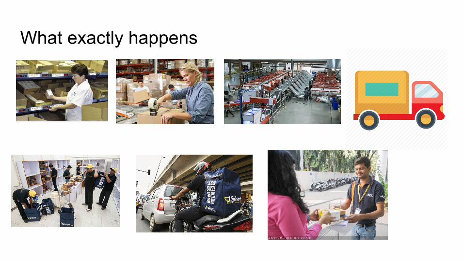
What exactly happens

DecisionsAre there any decisions to be made?

When should pick start in the FC? What is the order or batch for pick?

When should other activities be performed? Should items be held somewhere?

Which transport connection and mode should be taken?

Which route should be taken during transportation?

Do we really need to take these decisions? What happens if we process as and when order are placed or as and when shipments arrive at a particular location?

Transportation Schedule

Downstream Capacity

Storage Usage

➔ Hour 1 ◆ Operation-1 processes 75 small units. ◆ Operation-2 will be able to process 50 small units and remaining 25 will remain in storage.

➔ Hour 2 ◆ Operation-1 processes 50 large units. ◆ Operation-2 can processes these 50 large units plus 25 small present in storage.

➔ This average processing over two hours is 62 units and at the end of two hours storage is empty.

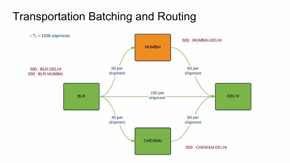
Transportation Batching and Routing

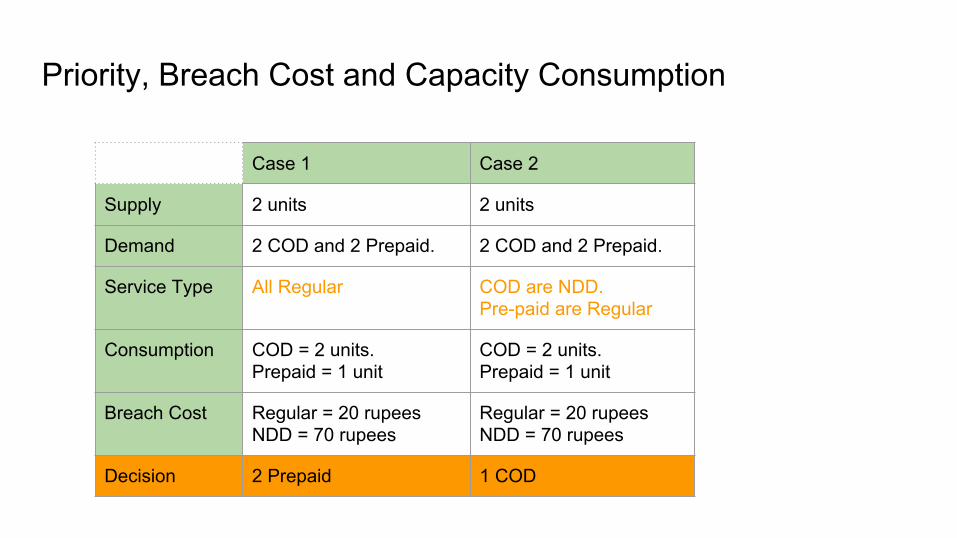
Priority, Breach Cost and Capacity Consumption

Case 1 Case 2

Supply 2 units 2 units

Demand 2 COD and 2 Prepaid. 2 COD and 2 Prepaid.

Service Type All Regular COD are NDD. Pre-paid are Regular

Consumption COD = 2 units. Prepaid = 1 unit

COD = 2 units. Prepaid = 1 unit

Breach Cost Regular = 20 rupeesNDD = 70 rupees

Regular = 20 rupeesNDD = 70 rupees

Decision 2 Prepaid 1 COD

Priority, Breach Cost and Capacity Consumption

➔ Consumption Factory vary as per Stage of processing◆ Sortation Station

● Size◆ FC

● Proximity to packing stations● Packaging Type

◆ Delivery Centre● Payment Type● Address Type

➔ Breach cost or Profit on timely delivery ◆ Service Type ◆ Customer Type

Gigantic Graph

➔ Items : Different dimensions, Volume and Weight → Different restrictions and shipping costs.

➔ Constraints◆ Transport Connection Time◆ Priority of Shipments◆ SLA

Need to do all this at Lowest Possible Cost

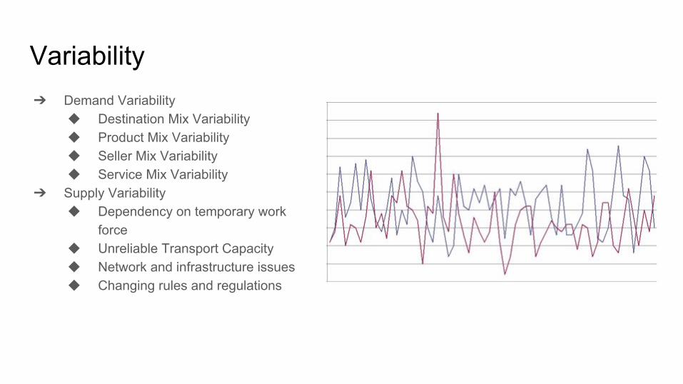
Variability➔ Demand Variability

◆ Destination Mix Variability◆ Product Mix Variability◆ Seller Mix Variability ◆ Service Mix Variability

➔ Supply Variability◆ Dependency on temporary work

force◆ Unreliable Transport Capacity◆ Network and infrastructure issues◆ Changing rules and regulations

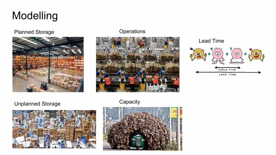
ModellingPlanned Storage

Unplanned Storage

Operations

Capacity

Lead Time

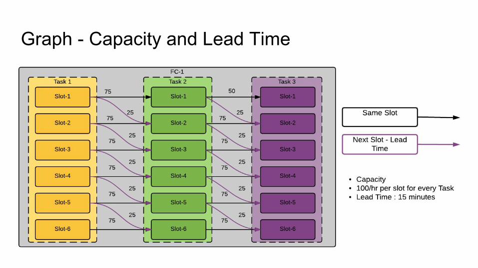
Graph - Capacity and Lead Time

Capacity Modelling with Storage

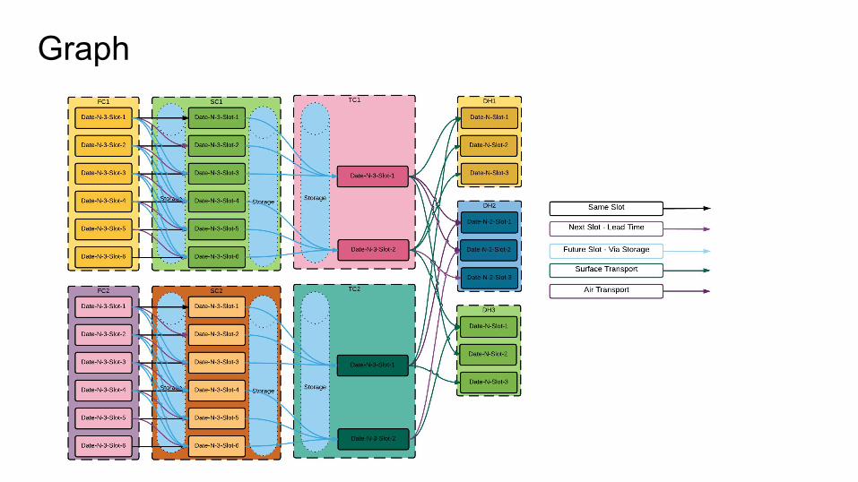
Graph

Plan Creation

➔ Computation Graph Creation➔ Start and Terminal Nodes Identification➔ Feasible Set ➔ Optimisation Function➔ Allocation➔ Learning➔ Usage of Learning➔ Repeat➔ Terminating Conditions➔ Match

Scalability➔ Nodes - Millions➔ Edges - Tens of millions➔ Need to distribute the

computation

Bulk synchronous parallel and Pregel➔ BSP system consists of

◆ Local Memory Transactions.◆ Message routing across Components.◆ Synchronisation

➔ Pregel - Inspired by BSP◆ Graph is divided into Partitions

◆ Algorithm is modelled as Computation

at Vertex and Message Passing across Vertices.

◆ Sequence of supersteps

Example

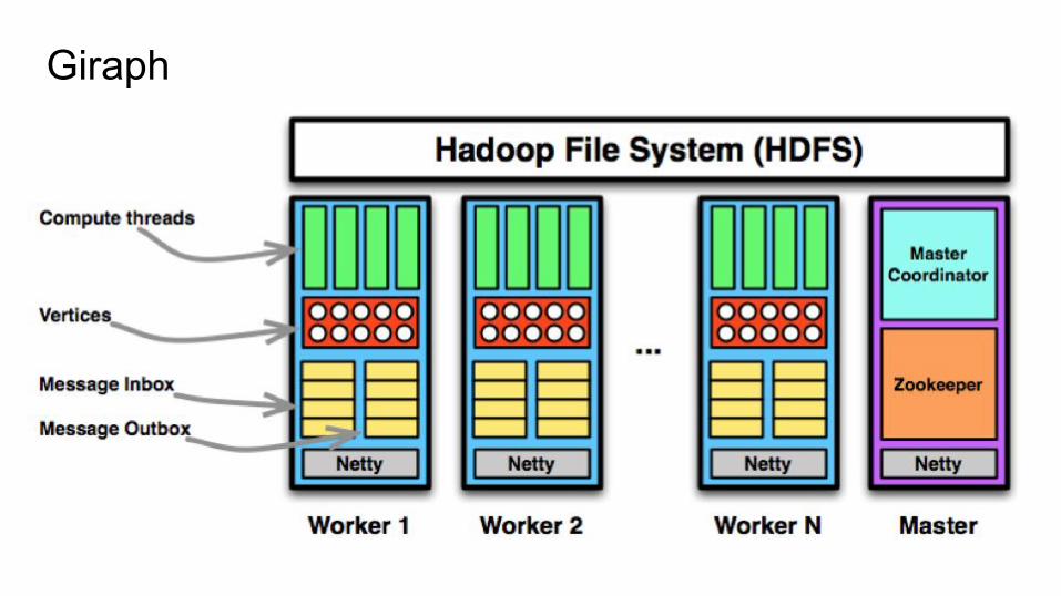
Giraph

Giraph Job Lifetime

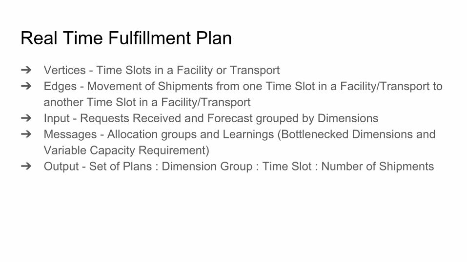
Real Time Fulfillment Plan➔ Vertices - Time Slots in a Facility or Transport➔ Edges - Movement of Shipments from one Time Slot in a Facility/Transport to

another Time Slot in a Facility/Transport➔ Input - Requests Received and Forecast grouped by Dimensions➔ Messages - Allocation groups and Learnings (Bottlenecked Dimensions and

Variable Capacity Requirement)➔ Output - Set of Plans : Dimension Group : Time Slot : Number of Shipments

Simulated Annealing - Global Optima and Local Optima➔ Starting with an initial solution. Learn better

allocation strategies. Move to a better neighbouring solution.

➔ It can lead to situations where you're stuck at a sub-optimal place.

➔ Simulated annealing injects right amount of randomness into things to escape local maxima.

Local PlanningOnce Global Plan is ready there are some local decisions to be taken. These do not affect the Global Plan and are hence taken independently

➔ Pick Path Optimisation➔ Sorting Configuration➔ Last Mile Vehicle Routing Problem

References➔ Distributed multi-agent optimization

◆ http://www.cds.caltech.edu/~murray/preprints/ttm11-ifac_s.pdf➔ Apache Giraph

◆ http://www.slideshare.net/ClaudioMartella/giraph-at-hadoop-summit-2014◆ http://giraph.apache.org/◆ http://www.apress.com/9781484212523

➔ BSP◆ https://en.wikipedia.org/wiki/Bulk_synchronous_parallel

➔ Reactive Search and Intelligent Optimization◆ REACTIVE SEARCH AND INTELLIGENT OPTIMIZATION Roberto Battiti, Mauro Brunato, and Franco Mascia

➔ Flow shop scheduling◆ http://faculty.ksu.edu.sa/ialharkan/IE428/Chapter_4.pdf◆ https://en.wikipedia.org/wiki/Flow_shop_scheduling

➔ Ant colony optimization◆ http://www.scholarpedia.org/article/Ant_colony_optimization◆ M. Dorigo, M. Birattari & T. Stützle, 2006 Ant Colony Optimization: Artificial Ants as a Computational Intelligence

Technique. TR/IRIDIA/2006-023➔ Simulated Annealing

◆ https://en.wikipedia.org/wiki/Simulated_annealing➔ Images have been picked by searching Google Images