REAL-TIME INTEGRATION OF RESERVOIR MODELING AND FORMATION TESTING

RR

SPWLA 50th Annual Logging Symposium, June 21-24, 2009

1

REAL-TIME INTEGRATION OF RESERVOIR MODELING AND FORMATION TESTING

Adriaan GISOLF, Francois X. DUBOST Julian ZUO, Schlumberger, Stephen WILLIAMS, StatoilHydro ASA, Julianne KRISTOFFERSEN,

Vladislav ACHOUROV, Andrawiss BISARAH, Oliver C. MULLINS Schlumberger

Society of Petrophysicists and Well Log Analysts

Copyright 2009, held jointly by the Society of Petrophysicists and Well Log Analysts (SPWLA) and the submitting authors. This paper was prepared for presentation at the SPWLA 50th Annual Logging Symposium held in The Woodlands, Texas, United States, June 21-24, 2009. ABSTRACT The increasing complexities of newly discovered reservoirs coupled with the increasing cost of field development mandate significantly improved and timely work flows for reservoir evaluation. Traditional modeling workflows are typically time consuming and require well-organized cross-disciplinary integration between geoscientists. Such models and processes are not well suited to be used and updated during formation-evaluation acquisition phases of field development. In this paper, a more accessible approach is proposed and demonstrated. The existing fluids model is combined with the current geologic model to construct an accurate representation of key features of the reservoir. This model is then used to predict data for a wireline formation sampling and testing tool (WFT), with emphasis on downhole fluid analysis (DFA). In this process, current reservoir understanding is tested by direct measurement in real time. If differences are uncovered between predicted and measured log data, the WFT tool is in the well, and measurements can be made to uncover the source of the error. In this paper a workflow is demonstrated in which WFT DFA and pressure/volume/temperature (PVT) lab reports were used to build a fluid model after the first exploration well data was acquired. This model was then used to predict fluid properties and WFT DFA logs for a subsequent well intersecting nominally the same compartment. These DFA predictions presumed fluid equilibrium and flow connectivity. Real-time comparisons were made of predicted and measured pressures, fluid gradients, contacts and DFA data obtained from the WFT logging run. Agreement of predicted and measured log data indicates that fluid properties and reservoir connectivities used for the modeling are correct. If predictions disagree with measurements, the acquisition program can be altered in real time to ensure sufficient data are acquired to understand the reservoir model inaccuracies.

During the WFT logging job, this predictive model enabled validation of critical WFT data. This process also allowed testing of the reservoir connectivity. It was discovered that either compartmentalization or lateral disequilibrium of the fluids in the reservoir exists. Interpretation of the DFA data suggested that a subtle lateral disequilibrium exists, and the assumption of reservoir connectivity is supported. INTRODUCTION As the search for hydrocarbons goes deeper and into more challenging reservoirs, greater reservoir complexity must be addressed. To properly evaluate such reservoirs continuously challenges formation-evaluation technology and techniques as well as economic limitations. It is essential to improve efficiency in this evolving setting. The existing workflows in reservoir evaluation offer opportunities for improvement. One area of potential improvement is identification of compartmentalization.[Mullins 2008, Mullins 2005, Elshahawi 2006, Elshahawi 2005] The extent of reservoir compartmentalization has a direct impact on the number of wells and the geometry and completion of those wells required to drain a reservoir, thereby greatly affecting the cost. Compartmentalization is very difficult to determine. Compartmentalization is best analyzed by history matching production over many years.[Dake 2001] However, this approach is simply not practical in most new oil fields because higher cost markets require huge capital expenditures prior to first oil. Well testing is also useful when identifying compartments; however, the large cost of such activities, especially offshore, precludes widespread use. Consequently, compartments must be identified without benefit of well testing. Compartments and DFA - There are a number of reasons why compartments are difficult to locate [Mullins 2008]. First, no formation evaluation measurements exist that can image (thin) sealing barriers at the reservoir length and scale. Methods incorporating DFA have proved the existence of compartments that are invisible to petrophysical well logging [Mullins 2008, Mullins 2005]. Second, the standard industry approach to compartment identification is to presume pressure communication

RR


2

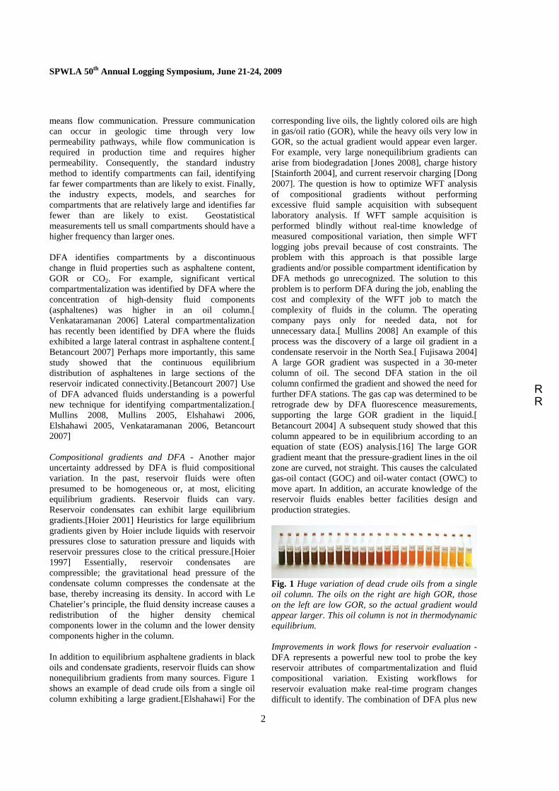
means flow communication. Pressure communication can occur in geologic time through very low permeability pathways, while flow communication is required in production time and requires higher permeability. Consequently, the standard industry method to identify compartments can fail, identifying far fewer compartments than are likely to exist. Finally, the industry expects, models, and searches for compartments that are relatively large and identifies far fewer than are likely to exist. Geostatistical measurements tell us small compartments should have a higher frequency than larger ones. DFA identifies compartments by a discontinuous change in fluid properties such as asphaltene content, GOR or CO2. For example, significant vertical compartmentalization was identified by DFA where the concentration of high-density fluid components (asphaltenes) was higher in an oil column.[ Venkataramanan 2006] Lateral compartmentalization has recently been identified by DFA where the fluids exhibited a large lateral contrast in asphaltene content.[ Betancourt 2007] Perhaps more importantly, this same study showed that the continuous equilibrium distribution of asphaltenes in large sections of the reservoir indicated connectivity.[Betancourt 2007] Use of DFA advanced fluids understanding is a powerful new technique for identifying compartmentalization.[ Mullins 2008, Mullins 2005, Elshahawi 2006, Elshahawi 2005, Venkataramanan 2006, Betancourt 2007] Compositional gradients and DFA - Another major uncertainty addressed by DFA is fluid compositional variation. In the past, reservoir fluids were often presumed to be homogeneous or, at most, eliciting equilibrium gradients. Reservoir fluids can vary. Reservoir condensates can exhibit large equilibrium gradients.[Hoier 2001] Heuristics for large equilibrium gradients given by Hoier include liquids with reservoir pressures close to saturation pressure and liquids with reservoir pressures close to the critical pressure.[Hoier 1997] Essentially, reservoir condensates are compressible; the gravitational head pressure of the condensate column compresses the condensate at the base, thereby increasing its density. In accord with Le Chatelier’s principle, the fluid density increase causes a redistribution of the higher density chemical components lower in the column and the lower density components higher in the column. In addition to equilibrium asphaltene gradients in black oils and condensate gradients, reservoir fluids can show nonequilibrium gradients from many sources. Figure 1 shows an example of dead crude oils from a single oil column exhibiting a large gradient.[Elshahawi] For the

corresponding live oils, the lightly colored oils are high in gas/oil ratio (GOR), while the heavy oils very low in GOR, so the actual gradient would appear even larger. For example, very large nonequilibrium gradients can arise from biodegradation [Jones 2008], charge history [Stainforth 2004], and current reservoir charging [Dong 2007]. The question is how to optimize WFT analysis of compositional gradients without performing excessive fluid sample acquisition with subsequent laboratory analysis. If WFT sample acquisition is performed blindly without real-time knowledge of measured compositional variation, then simple WFT logging jobs prevail because of cost constraints. The problem with this approach is that possible large gradients and/or possible compartment identification by DFA methods go unrecognized. The solution to this problem is to perform DFA during the job, enabling the cost and complexity of the WFT job to match the complexity of fluids in the column. The operating company pays only for needed data, not for unnecessary data.[ Mullins 2008] An example of this process was the discovery of a large oil gradient in a condensate reservoir in the North Sea.[ Fujisawa 2004] A large GOR gradient was suspected in a 30-meter column of oil. The second DFA station in the oil column confirmed the gradient and showed the need for further DFA stations. The gas cap was determined to be retrograde dew by DFA fluorescence measurements, supporting the large GOR gradient in the liquid.[ Betancourt 2004] A subsequent study showed that this column appeared to be in equilibrium according to an equation of state (EOS) analysis.[16] The large GOR gradient meant that the pressure-gradient lines in the oil zone are curved, not straight. This causes the calculated gas-oil contact (GOC) and oil-water contact (OWC) to move apart. In addition, an accurate knowledge of the reservoir fluids enables better facilities design and production strategies.

Fig. 1 Huge variation of dead crude oils from a single oil column. The oils on the right are high GOR, those on the left are low GOR, so the actual gradient would appear larger. This oil column is not in thermodynamic equilibrium. Improvements in work flows for reservoir evaluation - DFA represents a powerful new tool to probe the key reservoir attributes of compartmentalization and fluid compositional variation. Existing workflows for reservoir evaluation make real-time program changes difficult to identify. The combination of DFA plus new

RR


3

simplified workflows improves both reservoir evaluation and operational efficiency. If, for example, a model to be tested consists of one or a few connected sands with contained fluids in presumed equilibrium, then this is relatively simple to predict for DFA purposes, since all the complexity of the reservoir in the model is not needed. Knowledge of the connected formations and the general characteristics of the fluid are required. These simplifications enable timely DFA log predictions. In this paper, DFA log data and prior PVT data from an initial discovery well [Dubost 2007] are used to construct a simple fluid model that accounts for all properties measured by DFA. Only the fluid properties currently in the scope of DFA measurements are modeled. The model remains robust because it depends on previous DFA data. Predicting GOR from measured GOR is much easier than predicting phase boundaries from measured GOR. A simple, equilibrium fluid model is used to predict DFA data for presumably the same compartment but updip. That is, the key reservoir attribute of interest for DFA predictions is connectivity of the primary reservoir sand. In the future, this workflow can be expanded to include other log data to test more attributes of the geologic model. In this case study, the predicted log data were used to validate DFA log data. A problem with acquired DFA log data was uncovered and corrected. A unexpected observation was made regarding the GOC and indicated that either the reservoir fluid is in disequilibrium laterally or there is a compartment. The former explanation means little to field development; the latter would cause a significant undesired change in planning. A novel analysis of DFA log data coupled with recent development in the science of petroleum heavy ends suggests that connectivity prevails. Enabling measurement and sampling technologies - Wireline formation tester tools have been described in detail before [Schlumberger 2006], but some concepts key to the understanding of this paper are repeated here. DFA is a collective term used for in situ characterization of reservoir fluids within individual wells and collectively in many wells within a reservoir.[Mullins 2008] Since this paper contains extensive discussions on the measurements obtained with compositional fluid analyzers, one of the DFA tools, this warrants some further description of this concept. The compositional fluid analyzer measurements are based primarily on visible–near-infrared (Vis-NIR) absorption spectroscopy technology and can obtain formation fluid spectra in real time.[Mullins 2008, ,Mullins 2001, Dong 2002, Dong 2007] The vibrations of the chemical molecules or

groups, CH4, -CH3 and -CH2-, differ from each other essentially by virtue of their different mass (all mechanical oscillators have a similar mass dependence). Standard chemometric techniques enable analysis for three hydrocarbon chemical groups: C1, C2-C5, and C6+. In addition, CO2 can be measured by DFA methods because of its unique NIR signature.[Müller 2006] The GOR of the fluid is estimated from the derived hydrocarbon groups. A fluorescence detector is also present in the tool for a variety of purposes, such as retrograde condensate detection.[Betancourt 2004] When DFA is used to identify compositional variations within a continuous hydrocarbon column, it is important to eliminate any influence that the invaded mud filtrate may have on the formation fluid that is analyzed. Traditionally, this was done by pumping large volumes of formation fluid through a single probe mounted on a formation tester. The deeper the invasion of mud filtrate, the larger the volumes required. This technique usually resulted in acceptable levels of contamination if the invaded fluid and virgin fluid were nonmiscible. An example of such fluids is a water-based mud in a well drilled through an oil reservoir. In this case, the invaded fluid, water-based mud filtrate, does not dissolve in the native fluid. When pumping this fluid through a single probe, the fluids segregate when they reside in the pump [Betancourt 2004]. If a fluid analyzer is placed downstream from the pump, it is possible to analyze the slugs of virgin fluid, even in the presence of some mud filtrate. This phase segregation in the pumpout also applies to immiscible hydrocarbon phases and is a great aid in detection of liquid dropout from a retrograde condensate.[ Betancourt 2004]

When sampling miscible fluids it is practicably impossible to achieve zero-percent contamination. The lowest level of contamination that can be achieved is related to the ratio of vertical to horizontal permeability and to the viscosity contrast between the filtrate and the formation fluid. Extensive sampling experience with probe-type formation testers has shown that near-zero contamination results are only possible in the rare case of sampling very thin beds in high-mobility environments. If a conventional probe is used, it is essential to analyze the fraction of contamination in real time so that proper assessment can be made about when to acquire a sample and when to use DFA methods for reservoir evaluation. Estimating contamination in real time is accomplished by measuring the variation of color (asphaltene/resin content) and dissolved methane content along with application of a semi-empirical contamination equation.[Mullins 2001, Dong 2002]

RR


4

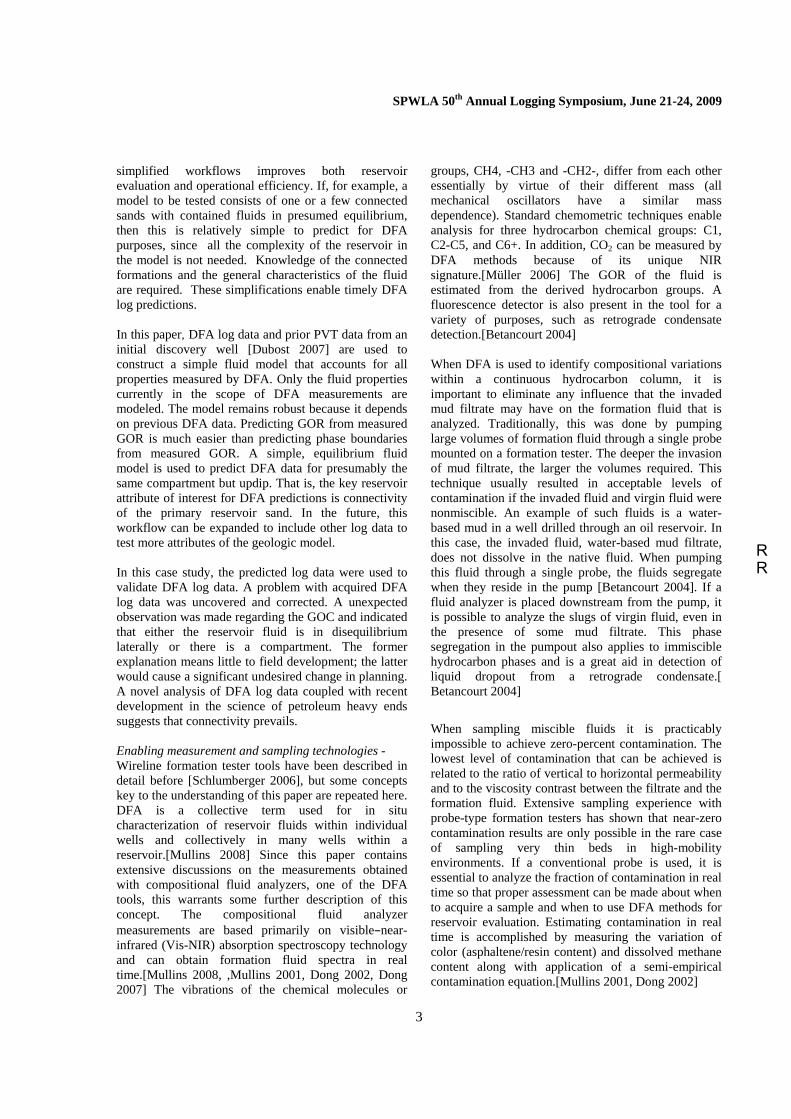
The preferred solution to miscible contamination is to get rid of it; this can be achieved with focused sampling. Focused sampling has been available for several years, and we describe the basics of operation here.[ Weinheber 2006, Del Campo 2006] Consider the schematic of the focused sampling probe shown in Figure 2. The probe has been separated into two distinct flow areas. There is an annular ring probe around the outside called the guard ring and a center probe for sample acquisition. There are two separate flowlines entering into the tool body as shown in Figure 2. The contamination is known to enter the WFT primarily in peripheral flow in the formation from along the borehole axis and from around the sides of the borehole. These fluids enter the guard probe. In contrast, fluids originating radially away from the borehole are virtually devoid of contamination after short pumping times and enter the sample probe. [Weinheber 2006, Del Campo 2006]

Fig 2 Focused sampling and flow regime.

MATHEMATICAL FORMULATION OF COMPOSITIONAL GRADIENTS

To calculate compositional gradients with depth in a hydrocarbon reservoir using EOS, it is usually assumed that all the components of reservoir fluids have zero mass flux, which is a stationary state in absence of convection. For a mixture with N-components, a set of flux equations are expressed as:

NiJJJJJ essurei

Thermali

Gravityi

Chemicalii ,...,2,1...,Pr =++++= (1)

where Ji is the flux of component i. The superscripts denote the fluxes due to chemical, gravitational, thermal, and pressure forces. We may add more flux terms in Eq. (1), such as active charging, sealing shale leaking, etc. At a stationary (steady) state, total flux of component i is equal to zero. If we take into account the driving forces due to chemical, gravitational, and thermal parts, the resulting equations are expressed as:

( ) NiTTF

gvMnn

N

j

Tiiij

nPTj

i

ij

,...,2,1,01 ,,

==∇+−−∇⎟⎟⎠

⎞⎜⎜⎝

⎛

∂∂

∑=

≠

ρμ (2)

where μi, ni, vi, Mi, g, ρ, and T are the chemical potential, the mole number, the partial molar volume, the molecular weight of component i, the gravitational acceleration, the density, and the temperature, respectively. FTi is the thermal diffusion flux of component i. Since the chemical potential is a function of pressure, temperature, and mole number, it can be expressed as at constant temperature:

( ) ∑=

∇⎟⎟⎠

⎞⎜⎜⎝

⎛

∂∂+∇⎟

⎠⎞

⎜⎝⎛∂∂=∇

≠

N

jj

nPTj

i

nT

iTi n

nP

Pij

1 ,,,

μμμ (3)

It is also assumed that the reservoir is in hydrostatic equilibrium, i.e.,

gP ρ=∇ (4) According to thermodynamic relations, partial molar volume is defined as:

nT

ii P

v,

⎟⎠⎞

⎜⎝⎛∂∂

=μ

(5)

Therefore, the chemical potential change at constant temperature is rewritten as:

( ) ∑=

∇⎟⎟⎠

⎞⎜⎜⎝

⎛

∂∂

+=∇≠

N

jj

nPTj

iiTi n

ngv

ij1 ,,

μρμ (6)

Substituting Eq. (6) into Eq. (2), we finally obtain:

( ) NiTTFgM Ti

iTi ,...,2,1=∇−=∇μ (7) The thermal diffusion flux of component i (FTi) can be calculated by different thermal diffusion models. An example is the Haase expression: [Haase 1971, Pedersen 2003]

⎟⎟⎠

⎞⎜⎜⎝

⎛−=

i

i

m

miTi M

HMH

MF (8)

where m stands for the property of the mixture. H is the molar enthalpy. Haase et al. (1971) assumed that the

RR


5

absolute enthalpy is equal to the residual enthalpy, i.e., ignoring ideal gas enthalpy. Hoier and Whitson (2000) used the model of Haase et al. to calculate the compositional gradients with depth in hydrocarbon reservoirs with a linear thermal gradient.[Hoier 2000] They concluded that a thermal gradient would weaken the compositional variation with depth in terms of the concept of Haase et al. To take into account the ideal gas enthalpy term, Pedersen and Lindeloff (2003) developed expressions for calculating enthalpy.[26] However, the values of ideal gas enthalpy for C3 and n-C4 are determined by optimizing absolute ideal gas enthalpy at 273.15 K and the value for C1 was arbitrarily set to zero. H values can be treated as adjustable parameters for pseudo components to match DFA data. Because of uncertainties in the thermal diffusion term, we assume that the reservoir is isothermal. The resulting equations are given by:

NiRT

gMh

f ii ,...,2,1,0ln ==−∂

∂ (9)

where fi is the fugacity of component i and h stands for the vertical depth. An EOS such as the Peng-Robinson EOS (1976) can be used to estimate fugacity of component i.[Peng 1976] Therefore, Eq. (9) is rearranged as:

( ) ( ) ( )Ni

RThhgM

PzPz ihiihii ,...,2,1,lnln 00

=−

=− ϕϕ (10)

where ϕi and zi are the fugacity coefficient and mole fraction of component i, respectively, and h0 denotes the reference depth. As shown in Eq. (10), the Peneloux volume shift [Peneloux 1982] will impact on compositional gradient calculations because the volume shift term in the fugacity coefficient of component i is expressed as:

RTPciEoSPROriginal

iEoSPRPeneloux

i −= ____ lnln ϕϕ (11)

where superscripts Peneloux_PR_EoS and Original_PR_EoS stand for the fugacity coefficients calculated by the PR EoS with and without the Peneloux volume shift, respectively and ci is the volume shift parameter of component i. Since P is different at h and h0, the volume shift terms cannot be canceled out in Eq. (10). To employ EOS to calculate fugacity coefficients and critical properties, acentric factors of components are required. The characterization procedure of Zuo and Zhang (2000) is applied to characterize single carbon

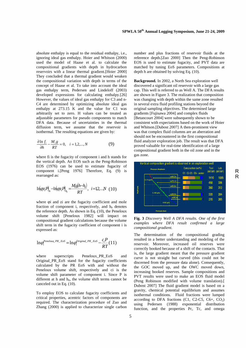
number and plus fractions of reservoir fluids at the reference depth.[Zuo 2000] Then the Peng-Robinson EOS is used to estimate fugacity, and PVT data are matched by tuning EoS parameters. Compositions at depth h are obtained by solving Eq. (10). Background. In 2002, a North Sea exploration well discovered a significant oil reservoir with a large gas cap. This well is referred to as Well A. The DFA results are shown in Figure 3. The realization that composition was changing with depth within the same zone resulted in several extra fluid profiling stations beyond the original sampling objectives. The determined large gradients [Fujisawa 2004] and complex fluids [Betancourt 2004] were subsequently shown to be consistent with expectations based on the work of Hoier and Whitson.[Dubost 2007] A then-prominent view was that complex fluid columns are an aberration and should not be encountered in the first compositional fluid analyzer exploration job. The result was that DFA proved valuable for real-time identification of a large compositional gradient both in the oil zone and in the gas zone.

Fig. 3 Discovery Well A DFA results. One of the first examples where DFA result confirmed a large compositional gradient.

The determination of the compositional grading resulted in a better understanding and modeling of the reservoir. Moreover, increased oil reserves were correctly booked because of a shift of the contacts. That is, the large gradient meant that the pressure gradient curve is not straight but curved (this could not be discerned from the pressure data alone). Consequently, the GOC moved up, and the OWC moved down, increasing booked reserves. Sample compositions and PVT results were used to make an EOS fluid model (Peng Robinson modified with volume translation).[ Dubost 2007] The fluid gradient model is based on a gravity, chemical potential equilibrium and assumes isothermal conditions. Fluid fractions were lumped according to DFA fractions (C1, C2-C5, C6+, CO2) using Pedersen (1988) exponential distribution function, and the properties Pc, Tc, and omega

RR


6

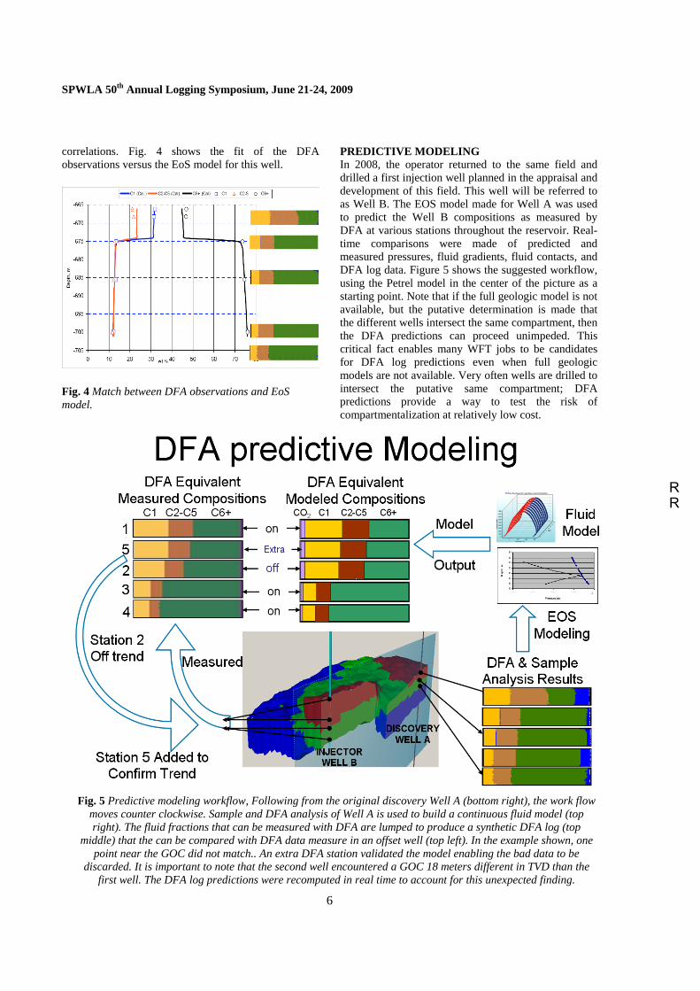
correlations. Fig. 4 shows the fit of the DFA observations versus the EoS model for this well.

Fig. 4 Match between DFA observations and EoS model.

PREDICTIVE MODELING In 2008, the operator returned to the same field and drilled a first injection well planned in the appraisal and development of this field. This well will be referred to as Well B. The EOS model made for Well A was used to predict the Well B compositions as measured by DFA at various stations throughout the reservoir. Real-time comparisons were made of predicted and measured pressures, fluid gradients, fluid contacts, and DFA log data. Figure 5 shows the suggested workflow, using the Petrel model in the center of the picture as a starting point. Note that if the full geologic model is not available, but the putative determination is made that the different wells intersect the same compartment, then the DFA predictions can proceed unimpeded. This critical fact enables many WFT jobs to be candidates for DFA log predictions even when full geologic models are not available. Very often wells are drilled to intersect the putative same compartment; DFA predictions provide a way to test the risk of compartmentalization at relatively low cost.

Fig. 5 Predictive modeling workflow, Following from the original discovery Well A (bottom right), the work flow moves counter clockwise. Sample and DFA analysis of Well A is used to build a continuous fluid model (top right). The fluid fractions that can be measured with DFA are lumped to produce a synthetic DFA log (top

middle) that the can be compared with DFA data measure in an offset well (top left). In the example shown, one point near the GOC did not match.. An extra DFA station validated the model enabling the bad data to be

discarded. It is important to note that the second well encountered a GOC 18 meters different in TVD than the first well. The DFA log predictions were recomputed in real time to account for this unexpected finding.

RR


7

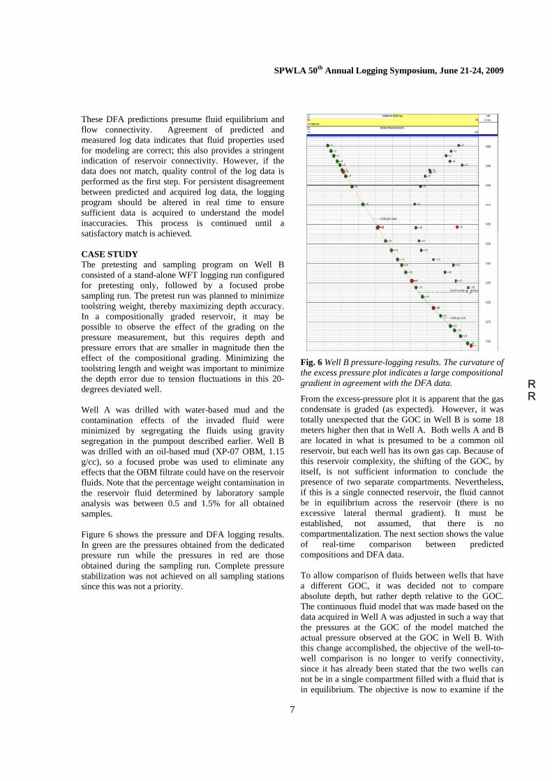
These DFA predictions presume fluid equilibrium and flow connectivity. Agreement of predicted and measured log data indicates that fluid properties used for modeling are correct; this also provides a stringent indication of reservoir connectivity. However, if the data does not match, quality control of the log data is performed as the first step. For persistent disagreement between predicted and acquired log data, the logging program should be altered in real time to ensure sufficient data is acquired to understand the model inaccuracies. This process is continued until a satisfactory match is achieved. CASE STUDY The pretesting and sampling program on Well B consisted of a stand-alone WFT logging run configured for pretesting only, followed by a focused probe sampling run. The pretest run was planned to minimize toolstring weight, thereby maximizing depth accuracy. In a compositionally graded reservoir, it may be possible to observe the effect of the grading on the pressure measurement, but this requires depth and pressure errors that are smaller in magnitude then the effect of the compositional grading. Minimizing the toolstring length and weight was important to minimize the depth error due to tension fluctuations in this 20-degrees deviated well. Well A was drilled with water-based mud and the contamination effects of the invaded fluid were minimized by segregating the fluids using gravity segregation in the pumpout described earlier. Well B was drilled with an oil-based mud (XP-07 OBM, 1.15 g/cc), so a focused probe was used to eliminate any effects that the OBM filtrate could have on the reservoir fluids. Note that the percentage weight contamination in the reservoir fluid determined by laboratory sample analysis was between 0.5 and 1.5% for all obtained samples. Figure 6 shows the pressure and DFA logging results. In green are the pressures obtained from the dedicated pressure run while the pressures in red are those obtained during the sampling run. Complete pressure stabilization was not achieved on all sampling stations since this was not a priority.

Fig. 6 Well B pressure-logging results. The curvature of the excess pressure plot indicates a large compositional gradient in agreement with the DFA data.

From the excess-pressure plot it is apparent that the gas condensate is graded (as expected). However, it was totally unexpected that the GOC in Well B is some 18 meters higher then that in Well A. Both wells A and B are located in what is presumed to be a common oil reservoir, but each well has its own gas cap. Because of this reservoir complexity, the shifting of the GOC, by itself, is not sufficient information to conclude the presence of two separate compartments. Nevertheless, if this is a single connected reservoir, the fluid cannot be in equilibrium across the reservoir (there is no excessive lateral thermal gradient). It must be established, not assumed, that there is no compartmentalization. The next section shows the value of real-time comparison between predicted compositions and DFA data. To allow comparison of fluids between wells that have a different GOC, it was decided not to compare absolute depth, but rather depth relative to the GOC. The continuous fluid model that was made based on the data acquired in Well A was adjusted in such a way that the pressures at the GOC of the model matched the actual pressure observed at the GOC in Well B. With this change accomplished, the objective of the well-to-well comparison is no longer to verify connectivity, since it has already been stated that the two wells can not be in a single compartment filled with a fluid that is in equilibrium. The objective is now to examine if the

RR


8

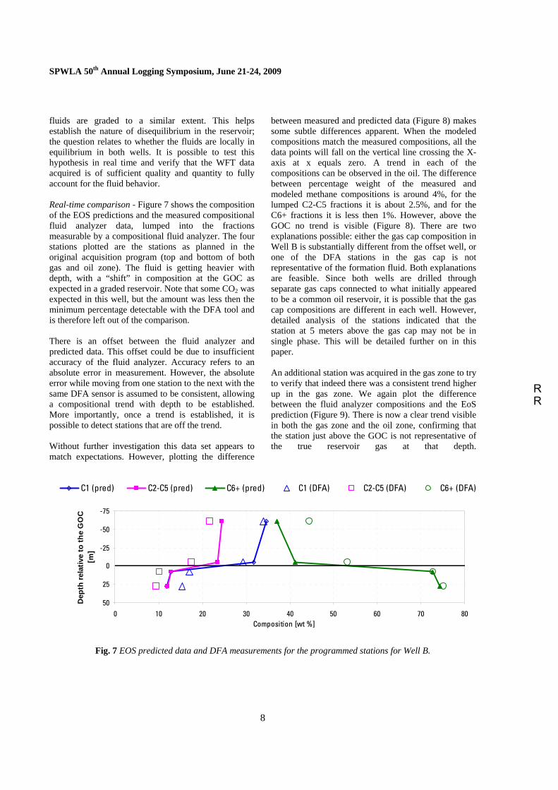
fluids are graded to a similar extent. This helps establish the nature of disequilibrium in the reservoir; the question relates to whether the fluids are locally in equilibrium in both wells. It is possible to test this hypothesis in real time and verify that the WFT data acquired is of sufficient quality and quantity to fully account for the fluid behavior. Real-time comparison - Figure 7 shows the composition of the EOS predictions and the measured compositional fluid analyzer data, lumped into the fractions measurable by a compositional fluid analyzer. The four stations plotted are the stations as planned in the original acquisition program (top and bottom of both gas and oil zone). The fluid is getting heavier with depth, with a “shift” in composition at the GOC as expected in a graded reservoir. Note that some CO2 was expected in this well, but the amount was less then the minimum percentage detectable with the DFA tool and is therefore left out of the comparison. There is an offset between the fluid analyzer and predicted data. This offset could be due to insufficient accuracy of the fluid analyzer. Accuracy refers to an absolute error in measurement. However, the absolute error while moving from one station to the next with the same DFA sensor is assumed to be consistent, allowing a compositional trend with depth to be established. More importantly, once a trend is established, it is possible to detect stations that are off the trend. Without further investigation this data set appears to match expectations. However, plotting the difference

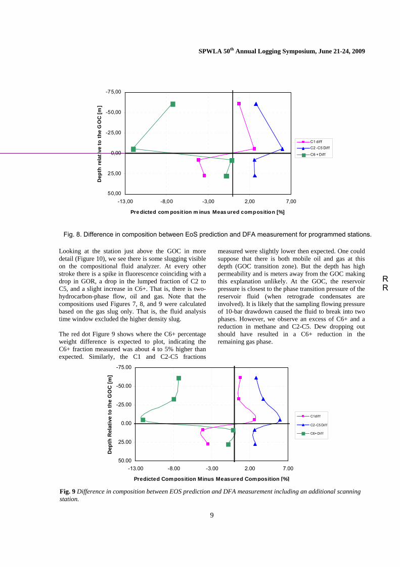
between measured and predicted data (Figure 8) makes some subtle differences apparent. When the modeled compositions match the measured compositions, all the data points will fall on the vertical line crossing the X-axis at x equals zero. A trend in each of the compositions can be observed in the oil. The difference between percentage weight of the measured and modeled methane compositions is around 4%, for the lumped C2-C5 fractions it is about 2.5%, and for the C6+ fractions it is less then 1%. However, above the GOC no trend is visible (Figure 8). There are two explanations possible: either the gas cap composition in Well B is substantially different from the offset well, or one of the DFA stations in the gas cap is not representative of the formation fluid. Both explanations are feasible. Since both wells are drilled through separate gas caps connected to what initially appeared to be a common oil reservoir, it is possible that the gas cap compositions are different in each well. However, detailed analysis of the stations indicated that the station at 5 meters above the gas cap may not be in single phase. This will be detailed further on in this paper. An additional station was acquired in the gas zone to try to verify that indeed there was a consistent trend higher up in the gas zone. We again plot the difference between the fluid analyzer compositions and the EoS prediction (Figure 9). There is now a clear trend visible in both the gas zone and the oil zone, confirming that the station just above the GOC is not representative of the true reservoir gas at that depth.

-75

-50

-25

0

25

500 10 20 30 40 50 60 70 80

Composition [wt %]

Dep

th re

lativ

e to

the

GO

C

[m]

C1 (pred) C2-C5 (pred) C6+ (pred) C1 (DFA) C2-C5 (DFA) C6+ (DFA)

Fig. 7 EOS predicted data and DFA measurements for the programmed stations for Well B.

RR


9

-75,00

-50,00

-25,00

0,00

25,00

50,00-13,00 -8,00 -3,00 2,00 7,00

Pre dicted com posit ion m inus Meas ured composition [%]

Dep

th re

lati

ve to

the

GO

C [m

]

C1 dif fC2 -C5 Dif f

C6 + Dif f

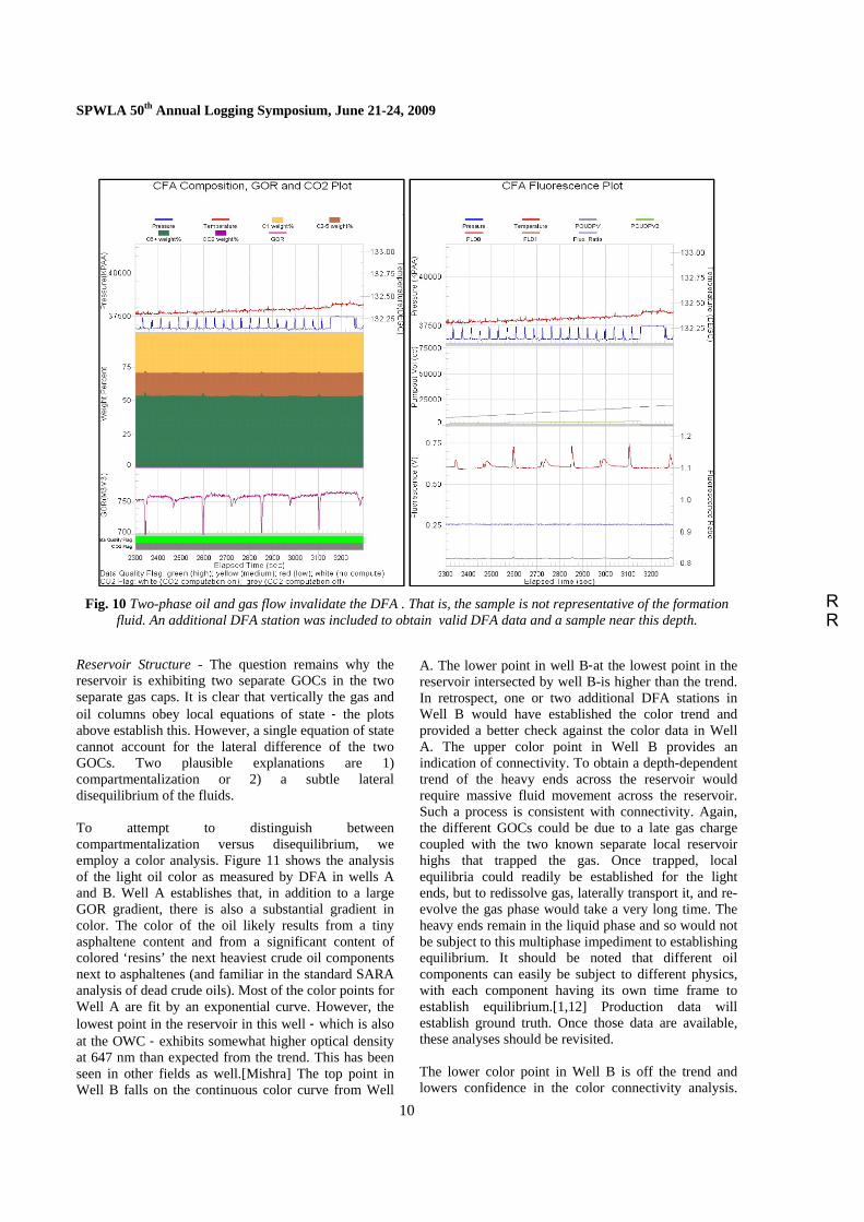
Looking at the station just above the GOC in more detail (Figure 10), we see there is some slugging visible on the compositional fluid analyzer. At every other stroke there is a spike in fluorescence coinciding with a drop in GOR, a drop in the lumped fraction of C2 to C5, and a slight increase in C6+. That is, there is two-hydrocarbon-phase flow, oil and gas. Note that the compositions used Figures 7, 8, and 9 were calculated based on the gas slug only. That is, the fluid analysis time window excluded the higher density slug.

The red dot Figure 9 shows where the C6+ percentage weight difference is expected to plot, indicating the C6+ fraction measured was about 4 to 5% higher than expected. Similarly, the C1 and C2-C5 fractions

measured were slightly lower then expected. One could suppose that there is both mobile oil and gas at this depth (GOC transition zone). But the depth has high permeability and is meters away from the GOC making this explanation unlikely. At the GOC, the reservoir pressure is closest to the phase transition pressure of the reservoir fluid (when retrograde condensates are involved). It is likely that the sampling flowing pressure of 10-bar drawdown caused the fluid to break into two phases. However, we observe an excess of C6+ and a reduction in methane and C2-C5. Dew dropping out should have resulted in a C6+ reduction in the remaining gas phase.

-75.00

-50.00

-25.00

0.00

25.00

50.00-13.00 -8.00 -3.00 2.00 7.00

Predicted Composition Minus Measured Composition [%]

Dep

th R

elat

ive

to th

e G

OC

[m]

C1 dif f

C2-C5 Dif f

C6+ Dif f

Fig. 9 Difference in composition between EOS prediction and DFA measurement including an additional scanning station.

Fig. 8. Difference in composition between EoS prediction and DFA measurement for programmed stations.

RR


10

Fig. 10 Two-phase oil and gas flow invalidate the DFA . That is, the sample is not representative of the formation

fluid. An additional DFA station was included to obtain valid DFA data and a sample near this depth.

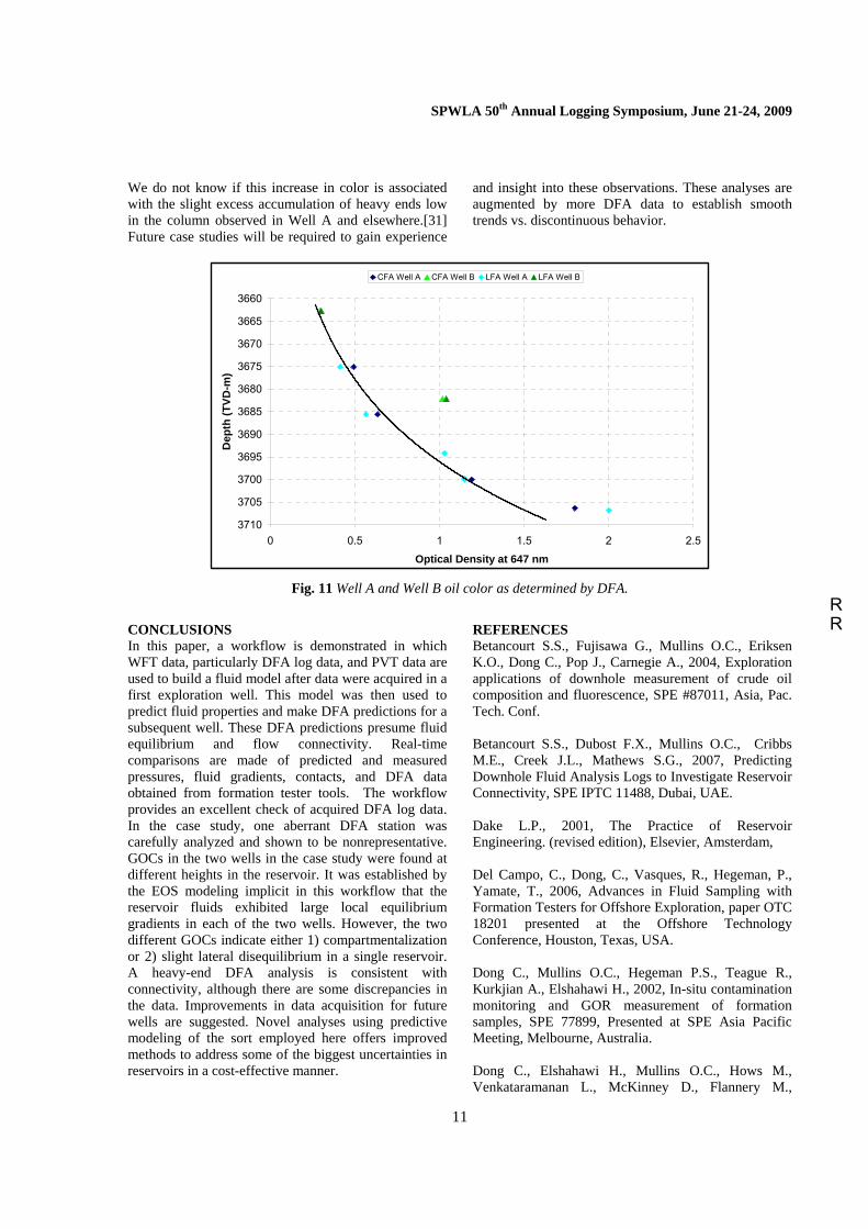
Reservoir Structure - The question remains why the reservoir is exhibiting two separate GOCs in the two separate gas caps. It is clear that vertically the gas and oil columns obey local equations of state - the plots above establish this. However, a single equation of state cannot account for the lateral difference of the two GOCs. Two plausible explanations are 1) compartmentalization or 2) a subtle lateral disequilibrium of the fluids. To attempt to distinguish between compartmentalization versus disequilibrium, we employ a color analysis. Figure 11 shows the analysis of the light oil color as measured by DFA in wells A and B. Well A establishes that, in addition to a large GOR gradient, there is also a substantial gradient in color. The color of the oil likely results from a tiny asphaltene content and from a significant content of colored ‘resins’ the next heaviest crude oil components next to asphaltenes (and familiar in the standard SARA analysis of dead crude oils). Most of the color points for Well A are fit by an exponential curve. However, the lowest point in the reservoir in this well - which is also at the OWC - exhibits somewhat higher optical density at 647 nm than expected from the trend. This has been seen in other fields as well.[Mishra] The top point in Well B falls on the continuous color curve from Well

A. The lower point in well B-at the lowest point in the reservoir intersected by well B-is higher than the trend. In retrospect, one or two additional DFA stations in Well B would have established the color trend and provided a better check against the color data in Well A. The upper color point in Well B provides an indication of connectivity. To obtain a depth-dependent trend of the heavy ends across the reservoir would require massive fluid movement across the reservoir. Such a process is consistent with connectivity. Again, the different GOCs could be due to a late gas charge coupled with the two known separate local reservoir highs that trapped the gas. Once trapped, local equilibria could readily be established for the light ends, but to redissolve gas, laterally transport it, and re-evolve the gas phase would take a very long time. The heavy ends remain in the liquid phase and so would not be subject to this multiphase impediment to establishing equilibrium. It should be noted that different oil components can easily be subject to different physics, with each component having its own time frame to establish equilibrium.[1,12] Production data will establish ground truth. Once those data are available, these analyses should be revisited. The lower color point in Well B is off the trend and lowers confidence in the color connectivity analysis.

RR


11

We do not know if this increase in color is associated with the slight excess accumulation of heavy ends low in the column observed in Well A and elsewhere.[31] Future case studies will be required to gain experience

and insight into these observations. These analyses are augmented by more DFA data to establish smooth trends vs. discontinuous behavior.

3660

3665

3670

3675

3680

3685

3690

3695

3700

3705

37100 0.5 1 1.5 2 2.5

Optical Density at 647 nm

Dep

th (T

VD-m

)

CFA Well A CFA Well B LFA Well A LFA Well B

Fig. 11 Well A and Well B oil color as determined by DFA.

CONCLUSIONS In this paper, a workflow is demonstrated in which WFT data, particularly DFA log data, and PVT data are used to build a fluid model after data were acquired in a first exploration well. This model was then used to predict fluid properties and make DFA predictions for a subsequent well. These DFA predictions presume fluid equilibrium and flow connectivity. Real-time comparisons are made of predicted and measured pressures, fluid gradients, contacts, and DFA data obtained from formation tester tools. The workflow provides an excellent check of acquired DFA log data. In the case study, one aberrant DFA station was carefully analyzed and shown to be nonrepresentative. GOCs in the two wells in the case study were found at different heights in the reservoir. It was established by the EOS modeling implicit in this workflow that the reservoir fluids exhibited large local equilibrium gradients in each of the two wells. However, the two different GOCs indicate either 1) compartmentalization or 2) slight lateral disequilibrium in a single reservoir. A heavy-end DFA analysis is consistent with connectivity, although there are some discrepancies in the data. Improvements in data acquisition for future wells are suggested. Novel analyses using predictive modeling of the sort employed here offers improved methods to address some of the biggest uncertainties in reservoirs in a cost-effective manner.

REFERENCES Betancourt S.S., Fujisawa G., Mullins O.C., Eriksen K.O., Dong C., Pop J., Carnegie A., 2004, Exploration applications of downhole measurement of crude oil composition and fluorescence, SPE #87011, Asia, Pac. Tech. Conf. Betancourt S.S., Dubost F.X., Mullins O.C., Cribbs M.E., Creek J.L., Mathews S.G., 2007, Predicting Downhole Fluid Analysis Logs to Investigate Reservoir Connectivity, SPE IPTC 11488, Dubai, UAE. Dake L.P., 2001, The Practice of Reservoir Engineering. (revised edition), Elsevier, Amsterdam, Del Campo, C., Dong, C., Vasques, R., Hegeman, P., Yamate, T., 2006, Advances in Fluid Sampling with Formation Testers for Offshore Exploration, paper OTC 18201 presented at the Offshore Technology Conference, Houston, Texas, USA. Dong C., Mullins O.C., Hegeman P.S., Teague R., Kurkjian A., Elshahawi H., 2002, In-situ contamination monitoring and GOR measurement of formation samples, SPE 77899, Presented at SPE Asia Pacific Meeting, Melbourne, Australia. Dong C., Elshahawi H., Mullins O.C., Hows M., Venkataramanan L., McKinney D., Flannery M.,

RR


12

Hashem M., 2007, Improved Interpretation of Reservoir Architecture and Fluid Contacts through the Integration of Downhole Fluid Analysis with Geochemical and Mud Gas Analyses, SPE 109683, APOGCE, Jakart Indonesia. Dong C., O'Keefe M., Elshahawi H., Hashem M., Williams S., Stensland D., Hegeman P., Vasques R., Terabayashi T., Mullins O.C., Donzier E., 2007, New Downhole Fluid Analyzer Tool for Improved Reservoir Characterization, Offshore Europe Conference, Aberdeen, Scotland, U.K., SPE 108566. Dubost F.X., Carnegie A.J., Mullins O.C., O’Keefe M., Betancourt S.S., Zuo J.Y., Eriksen K.O., 2007, Integration of In-Situ Fluid Measurements for Pressure Gradients Calculations, SPE 108494, Int. Oil Conf. Ex., Veracruz, Mexico. Elshahawi H., Hashem M.N., Mullins O.C., Fujisawa G., 2005, The missing link - identification of reservoir compartmentalization by downhole fluid analysis, SPE 94709 ATCE, Houston, TX. Elshahawi H., McKinney D., Flannery M., Mullins O.C., Venkataramanan L., Hasehm M., 2006, Compartmentalization revealed by Downhole Fluid Analysis coupled with Geochemistry, AAPG, Elshahawi H., Shell E&P Company Inc. Fujisawa G., Betancourt S.S., Mullins O.C., Torgersen T., O’Keefe M., Dong C., Eriksen K.O., 2004, Large Hydrocarbon Compositional Gradient Revealed by In-Situ Optical Spectroscopy, SPE 89704, ATCE, Houston, TX. Haase, R., Borgmann, H.-W., Ducker, K.H., and Lee, W.P., 1971, Thermodiffusion im Kritischen Verdampfungsgebiet Binarer Systeme, Naturforch, 26a, 1224-1227. Hoier L., 1997, “Miscibility Variations in Compositionally Grading Petroleum Reservoirs,” PhD thesis, Norwegian University of Science and Technology, Trondheim, Norway. Høier, L., and Whitson, C.H., 2000, Compositional Grading – Theory and Practice, SPE 63085, presented at 2000 SPE Annual Technical Conference and Exhibition, Dallas. Hoier L., Whitson C., 2001, “Compositional Grading, Theory and Practice,” SPEREE, 4(6), 525-535.

Jones D.M., Head I.M., Gray N.D., Adams J.J., Rowan A.K., Aitken C.M., Bennett B., Huang H., Brown A., Bowler B.F.J., Oldenburg T., Erdmann M., Larter S.R., 2008, Crude oil biodegradation via methanogenesis in subsurface petroleum reservoirs, Nature, 451, 176-180. Mishra , Zuo J., Dong C., Mullins O.C., private communication Müller N., Elshahawi H., Dong C., Mullins O.C., Flannery M., Ardila M., Weinheber P., McDade E.C., 2006, Quantification of carbon dioxide using downhole Wireline formation tester measurements, SPE 100739, SPE ATCE San Antonio, TX. Mullins O.C., Beck G., Cribbs M.Y., Terabayshi T., Kegasawa K., 2001, Downhole determination of GOR on single phase fluids by optical spectroscopy, SPWLA 42nd Annual Symposium, Houston, Texas, Paper M. Mullins O.C., Daigle T., Crowell C., Groenzin H., Joshi N.B., 2001 Gas-Oil Ratio of Live Crude Oils Determined by Near-Infrared Spectroscopy, Applied Spectros., 55, 197. Mullins O.C., Fujisawa G., Hashem M.N., Elshahawi H., 2005 Determination of coarse and ultra-fine scale compartmentalization by downhole fluid analysis coupled with other logs, International Petrol. Tech Conf. Paper 10036. Mullins O.C.,2008 The Physics of Reservoir Fluids; Discovery through Downhole Fluid Analysis, Schlumberger Press, Houston, TX, Pedersen, K.S., and Lindeloff, N., 2003, Simulations of Compositional Gradients in Hydrocarbon Reservoirs Under the Influence of a Temperature Gradient, SPE Paper 84364, presented at 2003 SPE Annual Technical Conference and Exhibition, Denver, Colorado. Peneloux, A., Rauzy, E., and Freze, R., 1982, A Consistent Correction for Redlich-Kwong-Soave Volumes, Fluid Phase Equilibria. Peng, D.-Y., and Robinson, D.B., 1976, A New Two-Constant Equation of State", Industrial Engineering Chemistry Fundamentals, Vol. 15, pp. 59-64. Schlumberger Marketing Communications, 2006, Fundamentals of formation testing, Schlumberger Press, Houston, TX. Stainforth J.G., 2004, “New Insights into Reservoir Filling and Mixing Processes” in J.M. Cubit, W.A. England, S. Larter, (Eds.) Understanding Petroleum

RR


13

Reservoirs: toward and Integrated Reservoir Engineering and Geochemical Approach, Geological Society, London, Special Publication. Venkataramanan L., Weinheber P., Mullins O.C., Andrews B., Gustavson G., 2006, Downhole Fluid Analysis with fluid comparison algorithms to identify reservoir compartmentalization, SPWLA, 47th Ann. Symp. Weinheber, P., and Vasques, R., 2006, New Formation Tester Probe Design for Low Contamination Sampling, Transactions of the SPWLA 47th Annual Logging Symposium, Veracruz, Mexico, paper Q. Zuo, J. Y., and Zhang, D., 2000, Plus Fraction Characterization and PVT Data Regression for Reservoir Fluids near Critical Conditions, SPE 64520, Presented at SPE Asia Pacific Oil and Gas Conference and Exhibition, Brisbane, Australia. ABOUT THE AUTHORS Adriaan Gisolf is a Reservoir Domain Champion with Schlumberger Norway. Previous positions held include Field Engineer in Indonesia and Nigeria, Service Quality Coach in Columbia and Reservoir Domain Champion in Angola. Francois X. Dubost is a Principal Reservoir Engineer with Schlumberger consulting services, based in Pau France. He began his career in 1995 with Wireline as a field engineer, then occupied operations management positions, before joining the technical community as reservoir domain champion. He has worked over the last two years in reservoir studies with the DCS segment, and holds an MSc Reservoir Engineering from Heriott Watt University, Scotland. Julian Zuo is Principle Chemical Engineer with DBR Technical Center, Schlumberger as Software Team Leader since 1998. Prior to that, he was a post-doctor and research associate at Technical University of Denmark and Ecole des Mines de Paris, France, each for 2 years. He received his PhD degree in Chemical Engineering in 1989 from University of Petroleum, China. He is an author and co-author of 40+ technical papers and made numerous presentations at the international conferences. Steve Williams is a petrophysics discipline leader with StatoilHydro located in Bergen, Norway. He is active in open and cased petrophysic logging/interpretation, formation testing and sampling. He holds MA in Natural Sciences from

Cambridge University, England 1984. Julianne Kristoffersen is working as a Reservoir Engineer for DCS in Stavanger. She began her career with Schlumberger in 2005 as a reservoir engineer with the consulting services group, also in Stavanger. She holds a Msc Reservoir Engineering from the Norwegian university of Science and technology. Vladislav Achourov has a Masters Degree in Physics from Gubkin State University of Oil & Gas, He has acquired 9 years working experience in the Oil and Gas industry in Schlumberger. The last 5 years he was leading solution implementations involving formation and well testing in Russia. Since 2008 he works as reservoir domain champion in Norway. Andrawiss Bisarah, Msc. Mechanical Engineering, was hired by Schlumberger in 2005 as a Wireline Field Engineer in the North Sea. He is now working in West Africa and leading an Ultra Deep offshore data acquisition campaign. Dr. Oliver C. Mullins, a chemist, is the primary originator of DFA and has authored a book on this topic (The Physics of Reservoir Fluids; Discovery through Downhole Fluid Analysis). He has been SPE Distinguished Lecturer and SPWLA Distinguished Lecturer on DFA. He is also active in asphaltene science and has coedited three books on this topic. He has coauthored 130 publications, and is coinventor on 51 allowed US patents.

Documents

REAL-TIME INTEGRATION OF RESERVOIR MODELING AND FORMATION TESTING