sensors

Article

Real-Time Lane Region Detection Using aCombination of Geometrical and Image Features

Danilo Cáceres Hernández, Laksono Kurnianggoro, Alexander Filonenko and Kang Hyun Jo *

Intelligent Systems Laboratory, Graduate School of Electrical Engineering, University of Ulsan, Ulsan 44610,Korea; danilo@islab.ulsan.ac.kr (D.C.H.); laksono@islab.ulsan.ac.kr (L.K.); alexander@islab.ulsan.ac.kr (A.F.)* Correspondence: acejo@ulsan.ac.kr; Tel.: +82-52-259-1664

Academic Editor: Felipe JimenezReceived: 28 August 2016; Accepted: 11 November 2016; Published: 17 November 2016

Abstract: Over the past few decades, pavement markings have played a key role in intelligent vehicleapplications such as guidance, navigation, and control. However, there are still serious issues facingthe problem of lane marking detection. For example, problems include excessive processing timeand false detection due to similarities in color and edges between traffic signs (channeling lines, stoplines, crosswalk, arrows, etc.). This paper proposes a strategy to extract the lane marking informationtaking into consideration its features such as color, edge, and width, as well as the vehicle speed.Firstly, defining the region of interest is a critical task to achieve real-time performance. In this sense,the region of interest is dependent on vehicle speed. Secondly, the lane markings are detected byusing a hybrid color-edge feature method along with a probabilistic method, based on distance-colordependence and a hierarchical fitting model. Thirdly, the following lane marking information isextracted: the number of lane markings to both sides of the vehicle, the respective fitting model, andthe centroid information of the lane. Using these parameters, the region is computed by using a roadgeometric model. To evaluate the proposed method, a set of consecutive frames was used in order tovalidate the performance.

Keywords: real-time lane region detection; collision risk region; lane marking hybrid-based strategy;hierarchical fitting model; distance-based color-dependent clustering

1. Introduction

The automotive industry is currently experiencing strong growth. Factors behind this areincreasing congestion, environmental issues, wireless network expansion, efficiencies in automotivelogistics, and demand for driver, passenger, and pedestrian safety. In that sense, advanced driverassistance systems (ADAS) have shown a very significant development since the early 1970s.ADAS focuses on vision-based applications, with examples including lane departure warnings, lanekeep assist, pedestrian detection, and collision avoidance. Although recent technological advancementsshow significant development results, there are still problems to solve. For example, actively-researchedproblems include gauging uncertainty in a static/dynamic environment, improving processing timeresponse, and managing road complexity.

Vision-based lane marking approaches focus primarily on the color-pattern changes betweenthe road surface and pavement marking materials [1–6]. This difference in color is used to detectlane markings by extracting the features, such as edge and color information. Once the lane markingfeatures are extracted, a model fitting is implemented taking into consideration the lane markinggeometry design, specifically width and length. Last but not least, processing time plays an importantrole in decision making. By considering color-based methods, researchers in [1–3] focused on the taskof lane marking detection using the HSI (hue, saturation, and intensity) color model. The algorithmicstrategy proposed by the authors [1,2] shows good performance in detection and processing time.

Sensors 2016, 16, 1935; doi:10.3390/s16111935 www.mdpi.com/journal/sensors

Sensors 2016, 16, 1935 2 of 19

However, this algorithm extracts the lane marking using only the color information belonging to themarkings, which is not accurate enough considering that there is a wide range of traffic signals onthe road with the same color information (crosswalk, stop lines, one-way streets, merging/divergingtraffic, etc.) without also taking into consideration the noise information (spilled paint on the roador surface with colors that belong to the lane marking). Researchers in [3] proposed a high-precisionlane-level localization using a stereo camera. After the rectification between stereo images is finished,the algorithm uses the intensity value from HSI color space, and then the edge information is extracted.Unlike the previously mentioned research, these authors proposed additional detectors in order toavoid false detection (humps, crosswalks, traffic word signals, arrows). Once the edges are extracted,the authors proposed a hyperbola fitting to search the pixels belonging to the lane marking withinthe image. To solve vehicle localization problems, the authors use the random sample consensus(RANSAC) algorithm. Although the algorithm provides a good estimate of reliability due to thedeveloped strategy, integration of these steps is time consuming.

Researchers in [4,5] give examples of edge-based methods. Mammeri et al. [4] proposed a lanemarking localization by combining the maximally stable extremal region (MSER) and Hough transform(HT). MSER is used to extract the stable region given by lane markings, traffic signs, etc. Once theregions are extracted, the algorithm refines the previous results. Here, the task entails line detectionusing a probabilistic progressive Hough transform to extract the line segments with a minimumrequired length. Then, the line segments within 10◦ and 85◦ are considered lane marking candidates,and the rest of the segments are removed. The proposed method shows reliable results; however, giventhat they depend on the environment, the algorithm’s response is not stable (Tables 3 and 4 in [4]).Additionally, the strategy is only suitable for a straight lane marking regions with a low velocity andhigh camera frame rate constraints. Researchers in [5] proposed an efficient lane detection methodusing spatiotemporal images. After the alignment between the frames is performed, the lane pointsare detected using the most dominant straight line defined by the HT. Then, a weighted least-squaresfitting is used as a fitting model. The algorithm has good performance with high processing time.Similarly, as gauged by authors in [1,2], the algorithm shows some error in regions such as bumps.

Researchers in [7] introduced a laser scanner application to estimate the vehicle heading angle.To do that, the authors proposed identifying the lane within the road surface by finding differencesbetween road and marking materials. Consequently, the lane region, the lane marking, the centroidof the lane width, the road geometry as well the vehicle heading angle are iteratively estimated.Firstly, for a laser line-scanner input range data, the set of points within the region of interest isextracted. The region of interest is defined as 20 m × 4 m, the square box is located 10 m to the leftand right of the laser sensor and between 10 m and 14 m in front of the laser. Secondly, in order todetect the road surface, an unsupervised density-based spatial clustering is implemented. As a result,the number of lanes within the road are detected. Thirdly, the lane markings are detected to improvethe accuracy of the previous step. This is done by finding the discontinuity caused by the changebetween surface, road to lane marking or vice-versa. Fourthly, the centroid of the lane is the centerpoint computed as the difference between the left and right lane marking located ahead of a vehicle(lane width). Fifthly, using the centroid information, the road geometry parameters are extracted; thedeflection angle θ, the chord length da, and the vehicle heading angle δ are computed. Although thealgorithm shows a good performance and accuracy, it may encounter problems in regions where lanemarkings are considerably deteriorated.

All the research introduced above shows reliable results for use in the field of advanced driverassistance systems or autonomous navigation. However, all of these methods are still facing problems,either in processing time or performance. Consequently, in order to improve the current algorithms,a vision-based real-time lane detection algorithm is proposed for application in intelligent vehicles.In that sense, the presented method does not just take into consideration the features of color, edge, andlength lane marking information, but also combines them, resulting in a speed-dependent, color-edgehybrid lane marking detection algorithm.

Sensors 2016, 16, 1935 3 of 19

To summarize, the main steps of the proposed method are described below. Regions withinthe image are classified into categories of collision risk, zero collision risk, and regions above thehorizon. The proposed algorithm focuses primarily on the collision risk region, which is extractedtaking into account the vehicle speed (considered as an important key), and the region of interest(ROI) increases as the speed increases and vice versa. The color and edge lane marking featuresare extracted by analyzing the color and width information. Then, by combining both features, themidpoints of the lane markings are extracted. This process plays an important role, and, because ofthis strategy, the midpoints are extracted if they belong to lane marking types; otherwise, no actionis carried out. In essence, other marking types such as crosswalks, line stops, and traffic signals onthe road surface are rejected. The algorithm is not sensitive to these types of marking. This strategyreflected a substantial decrease in processing time compared with the current lane marking algorithms,in which additional processing should be performed in order to remove the noise given by differenttypes of markers. Then, using the midpoint features, a hierarchical fitting model is implemented.A lane marking detection algorithm that solely relies on a line fitting model is not strong enough dueto various road environment scenarios. On the other hand, based on the processing time as well asthe road geometry design, implementation of a polynomial fitting model along the vehicle trajectoryis not the best solution. Using the proposed sensor setup, it was observed that around 5% of thelane markings within the image can be defined using a curve fitting model, while a line fitting modelshould be used for the rest. Consequently, to solve this problem, a hierarchical line/curve fitting modelhas been proposed. These strategies allow the algorithm to avoid the use of expensive computationwhen it is not required. Finally, the lane region is estimated by using the line/curve fitting parameters.

2. System Overview

Figures 1 and 2 show the sensor configuration used to gather the road imagery data, as well asthe vehicle platform. The camera is located at a height of 1.8 m and tilted down at an angle of 9◦ withrespect to the horizontal projection, 2.3 m from the vehicle front bumper, and 0.5 m to the right of thevehicle centerline.

Figure 1. Vehicle data acquisition platform. (a) shows the lateral view of the vehicle; (b) shows thefront view of the vehicle; and (c) shows the sensors located at the top of the vehicle at a height ofapproximately 1.8 m. The vehicle platform was equipped with Point Grey BlackFly cameras (PointGrey Research Inc., Richmond, BC, Canada) and a laser SICK Laser Measurement Sensor (SICK Ltd.,Richmond Hill, ON, Canada).

Assuming the vehicle undergoes planar motion, the geometry of the model is described as follows:h is the height of the camera above the ground, d is the distance between the camera at ground leveland the point P(x, y, z) in the real world, R(xc, yc) is the point P(x, y, z) projected to the center positionof the image plane through the optical axis of the camera, T(dx, dy, dz) is the centroid of the lane atthe ground level, γ is the angle between the optical axis of the camera and the horizontal projection,α is the angle formed by scanning the image from top to bottom with respect to the center point ofthe image R(xc, yc), yi|i = 1, . . . , 256 is the pixel position located at xc, (xc, yc) is the pixel located atthe center of the image plane, fp is the focal length in pixels, fmm is the focal length in millimeters,Iw is the image width in pixels, and Smm is the CCD or CMOS image sensor width in millimeters.The vehicle data were acquired by a National Instrument PXI Express module (National Instruments

Sensors 2016, 16, 1935 4 of 19

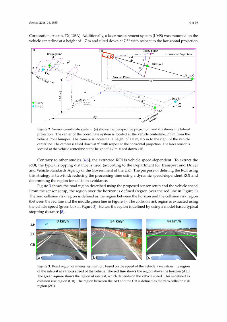
Corporation, Austin, TX, USA). Additionally, a laser measurement system (LMS) was mounted on thevehicle centerline at a height of 1.7 m and tilted down at 7.5◦ with respect to the horizontal projection.

Figure 2. Sensor coordinate system. (a) shows the perspective projection; and (b) shows the lateralprojection. The center of the coordinate system is located at the vehicle centerline, 2.3 m from thevehicle front bumper. The camera is located at a height of 1.8 m, 0.5 m to the right of the vehiclecenterline. The camera is tilted down at 9◦ with respect to the horizontal projection. The laser sensor islocated at the vehicle centerline at the height of 1.7 m, tilted down 7.5◦.

Contrary to other studies [4,6], the extracted ROI is vehicle speed-dependent. To extract theROI, the typical stopping distance is used (according to the Department for Transport and Driverand Vehicle Standards Agency of the Government of the UK). The purpose of defining the ROI usingthis strategy is two-fold: reducing the processing time using a dynamic speed-dependent ROI anddetermining the region for collision avoidance.

Figure 3 shows the road region described using the proposed sensor setup and the vehicle speed.From the sensor setup, the region over the horizon is defined (region over the red line in Figure 3).The zero collision risk region is defined as the region between the horizon and the collision risk region(between the red line and the middle green line in Figure 3). The collision risk region is extracted usingthe vehicle speed (green box in Figure 3). Hence, the region is defined by using a model-based typicalstopping distance [8].

Figure 3. Road region of interest estimation, based on the speed of the vehicle. (a–c) show the regionof the interest at various speed of the vehicle. The red line shows the region above the horizon (AH).The green square shows the region of interest, which depends on the vehicle speed. This is defined ascollision risk region (CR). The region between the AH and the CR is defined as the zero collision riskregion (ZC).

Sensors 2016, 16, 1935 5 of 19

3. Proposed Method

A method to detect the lane region in real-time using a multi-feature extraction based on a vehiclespeed-dependent strategy is introduced. Figure 4 shows the flow diagram of the proposed approach.The algorithm starts by extracting the ROI for a given input image using the current vehicle speedinformation. Then, the color and edge features are extracted, and are subsequently used in a hybridmethod to extract the midpoint within the lane marking candidate. Once the midpoints are extracted,a distance-based color-dependent clustering model is applied. Hence, a fitting model is used to extractthe lane marking for both lines and curves. Lastly, the centroid information, as well as the lane markingposition within the image, are extracted. Finally, using the previous extracted information, the laneregion is defined by computing the road geometry model. Therefore, this study aimed to detect thelane region for intelligent vehicle applications in which real-time decision making is required.

Figure 4. Flow diagram of the real-time lane region detection based on multi-features using a monocularcamera from a frame. (a) shows the input color image; (b) shows the result of the region of interestextraction. The section of the image above the red line indicates the horizon region. The zero collisionrisk region is located between red line and the green square. The region within the green square isthe collision risk region (dependent on vehicle speed), the region used in this approach; (c) shows thelane marking feature extraction. The top image shows the result of extracting the edge by using Otsu’sthresholding method. The bottom image shows the binary image result of extracting by using a colorprobability strategy; (d) shows the midpoints extraction method, a hybrid method which combinesboth the color and edge features; (e) shows the clustering result using a distance-based color-dependentmethod; (f) shows the fitting result. For each detected cluster, the best fitting line model is computed.Then, if the sum of the distance errors between the fitting line and the cluster is less than or equal to15 pixels, a straight lane marking was detected; otherwise, a curve fitting model is implemented usingthe Lagrangian interpolation polynomial approximation; (g) shows the result of the centroid as well asthe lane marking ending points extraction; and (h) shows the result of the road geometry estimationfor the current frame using the centroid information.

Sensors 2016, 16, 1935 6 of 19

3.1. Lane Marking Estimation

A vision-based lane marking detection method was introduced by Cáceres et al. in [8]. The authorspresented the results for the lane marking estimation using a monocular camera. Firstly, the horizonis defined off-line by using the trigonometric relationship between the camera and the target(see Figures 1 and 2). Secondly, the ROI is extracted by using the vehicle typical stopping distance.It should be noted that the region which belongs to the collision risk region is used in the ROIin this approach, as shown in Figures 3 and 4. The remaining regions will be used in furtherresearch. Thirdly, after the ROI has been defined, the edges are extracted using the red channel;this is because both yellow and white lane markings show a good contrast in the red channel [9,10].This is accomplished by using Otsu’s method [11] and a statistical threshold-dependent parameter.The statistical threshold-dependent parameter helps the algorithms to deal with problems arisingin the presence of shadows or other artifacts, as long as they do not appear within the image overa long period of time. Then, the edges are extracted using the Canny edge detector [12]. Fourthly,color pixels that belong to the lane marking are extracted. To do this, the probability density function(PDF) for the lane marking is created. The PDF is built for the cases of lane marking with or withoutpresence of shadows using the red, green, and blue (RGB) color model and the saturation (S) from thehue, saturation, and value (HSV) color model. Then, the intersection is performed using the detectionfrom each channel. Using the intersection result, the binary mask is created. As a result, for each lanemarking color type (white and yellow), a mask is extracted. Finally, both masks are combined using theunion between them. Fifthly, a lane marking hybrid-based strategy was implemented. The idea relieson the use of both the edge and color image results to extract the midpoint candidate. It is assumedthat for each lane marking, there is a midpoint along the x-axis. The proposed strategy is describedbelow. The image is scanned horizontally every p pixels along the y-axis; in the current algorithm,p is set to 3. The middle points between the consecutive edge points are extracted. Then, a BooleanAND operation is performed between the mid-point candidate and the color mask image. For allthe returned true values, the pixel coordinate position is stored. Finally, to define the set of clusters,a line-based color strategy is introduced in this approach. The distance, as well as line parameters areextracted for all of the mid-point candidates. Sixthly, at this step, all of the clusters are defined. Hence,the task consists of defining the function for each given cluster for both the line and curve models.Focusing on implementing a real-time application, a hierarchical fitting model is proposed instead ofusing a multi-fitting model [13]. First, for each cluster, a linear model is computed. Two points arechosen randomly at each iteration (n), where n is computed using the total amount of points (TAP)within the cluster, computed as follows: n = TAP

2 . Then, the sum of the error distances is computedfor all of the line fittings. The smallest error is chosen as the best fit if and only if the error is less than15 pixels; otherwise, the curve fitting model is computed based on an algebraic property of Lagrangianinterpolation polynomial approximation. Figure 5 shows the proposed lane marking strategy results(for more details, see Cáceres et al. in [8]).

Sensors 2016, 16, 1935 7 of 19

Figure 5. Lane marking results. (a–e) show a set of input images captured along the vehicletrajectory and their respective result of each step (from 1 to 7). The first row shows the input images.The second row shows the region of interest extraction using the speed of the vehicle. The third andfourth rows show the edge and color mask results. The fifth row shows the middle point extraction.The sixth row shows the clustering results. The seventh row shows the line/curve fitting model results.

3.2. Lane Region Detection

At this step, the lane markings are described using line/curve fitting models. In that sense, theline/curve parameters are stored, as well as the points located at the top and bottommost part of theimage. Therefore, the purpose of this step is to estimate the number of lane markings to each side ofthe vehicle and the centroid of the lane road. Since the fitting was already computed, the parametersfor each line/curve are already known. Furthermore, in this approach the distance between the fittingmodel and the bottom center part of the image is computed. To this end, the nearest fit models arechosen, one to each of the left and right sides, as well as the pixel positions located at the top-most andbottom-most parts of the image. Figure 6 shows the result of this step.

Figure 6. Centroid and lane marking ending points extraction. (a–d) show the result of the pointextraction for a set of frames. Points in white show the centroid of the lane region. Points in magentaand black show the top and bottom pixel position, respectively, for each detected line/curve. Points inred show the center at the bottommost part of the image used to estimate the shortest distance.Lines in yellow show the nearest distance to the left and right side. Lines in orange show the largestdistance to the left and right side.

Once the centroid of the lane within the image is extracted (a pixel coordinate), the next stepentails estimating the 3D coordinate at the ground level. To compute the distance using a monocularcamera, several approaches have been proposed, for example by authors in [14–17]. To estimate thedistance in this study, the method proposed by Fernandes et al. [17] was used, to compute the centroid.Then, the centroid position of the lane and the the lane marking points located at the topmost part andbottommost part of the lane marking were computed as follows:

α =yc − yt

fp; β =

xc − xt

fp, (1)

Sensors 2016, 16, 1935 8 of 19

dy =h

tan(γ + α), (2)

dx =dy cos(α) tan(β)

cos(γ + α), (3)

where fp, α, β, γ, dy, dx, R(xc, yc), T(xt, yt) are described in the system overview section (see Figure 2).Then, the next step consists of extracting the lane region detection following the circular motion criteria.The task consists of calculating the curvature of the circle model. To do that, the distance ahead of thevehicle as well as the heading angle formed between the centroid of the lane (previously computed)and the vehicle rear-axle should be computed. This is computed geometrically using the model shownin Figure 7, as follows:

da =√

x2t + (yt + 1.6)2, (4)

d1 = d2,

X = − x2t + (yt + 1.6)2

2xt,

r = d1 = d2 = |X|,

θ = 2δ ; δ = sin−1(

da

2r

), (5)

where da is the Euclidean distance between the point T(xt, yt) and the rear-axle position locatedat A(0,−1.6), and d1 and d2 are the distances between the center of the circle model (called theinstantaneous center of rotation (ICR)) and the target point T(xt, yt) and the rear-axle point A(0,−1.6),respectively; here, both distances refer to the radius r, while θ is the deflection angle (which refers tothe road geometry), and δ is the vehicle heading angle.

Figure 7. Road geometry model.

4. Experiments

The program was built in C++ and compiled in Ubuntu 12.04 using an Intel Core i7-4770 CPU,3.40 GHz, with 8 GB of RAM. A total of 3781 frames with a total of 8617 lane markings were used, withsingle, double and broken lane markings on both straight and road scenes. The image size used in thisalgorithm was 256 × 204. The camera sensor was mounted at the top of the vehicle at 1.8 m and tilteddown 9◦. The vehicle moves in a speed range of [5–45] km/h, acquired by a National Instrument PXIExpress module. The algorithm was tested using images gathered at the Korea Automobile Testing& Research Institute (KATRI), and they contain sand, bushes, and barriers, as well as spilled whitepaint along the lane markings. To test the algorithm, statistical analysis was performed to verify thereliability of the proposed method.

Sensors 2016, 16, 1935 9 of 19

4.1. Lane Marking Evaluation

This task consists in evaluating the lane marking result of the proposed algorithm with respect tothe lane marking ground truth (manually labeled). In essence, the evaluation describes the feasibilityof the proposed lane marking detection strategy—in other words, how effectively the lane markingalgorithm is able to detect correctly or remove lane marking candidates from the region of interest usingthe proposed hybrid color-edge feature method along the distance-color dependence probabilisticmethod and the hierarchical fitting model explained in Section 3.1 (see Figure 8). The road surfacedata, tested in this approach, has the following characteristics: double lane marking to the left andsingle lane marking to the right, single lane marking to both sides, single lane marking to the left andbroken double lane marking on the right side, single lane marking to the left and channelizing lanemarkings to the right.

Figure 8. False positive and negative results. The left image shows a false positive case where therightmost lane marking in cyan was detected due to the fact that the midpoints from the sand regionwere extracted as candidates in Section 3.1 steps three and four (see Figures 5 and 9 rows 3, 4 and 5).The last two images show the case of a false negative; in this case, tracking using the previous line/curvefit model is implemented. The line in red shows the results of the tracking, while the magenta showsthe results for the curve fitting. In the middle image, the false negative result was due to the fact thatthe lane marking edges were outside the range during the midpoint extraction process. This happenedbecause there was spilled paint along the lane marking. In the case of the right image, the algorithmwas not able to detect the lane marking because of the deterioration of the markers.

To evaluate the lane marking results, sensitivity (St), specificity (Sp), accuracy (A), and the falsepositive (FPs) and negative frames per second (FNs) rate metrics were used. The sensitivity measuresthe correct detection of the candidate as a lane marking, while the specificity measures the correctrejection of the false candidate as a non-lane marking. The accuracy describes how well the presentedmethod correctly classifies the lane marking. FPs and FNs indicate the amount of false positives ornegatives that occur in a second. They are computed as follows:

St =TP

TP + FN; Sp =

TNTN + FP

; A =TP + TN

TP + FP + FN + TN, (6)

FPs =FP ∗ PT

TF; FNs =

FN ∗ PTTF

, (7)

where TP (true positive) indicates that candidates are correctly detected, TN (true negative) indicatesthat candidates are correctly rejected, FN (false negative) indicates that lane markings were incorrectlyrejected, and FP (false positive) indicates that lane markings were incorrectly identified, TF is the totalamount of frames, PT is the processing time.

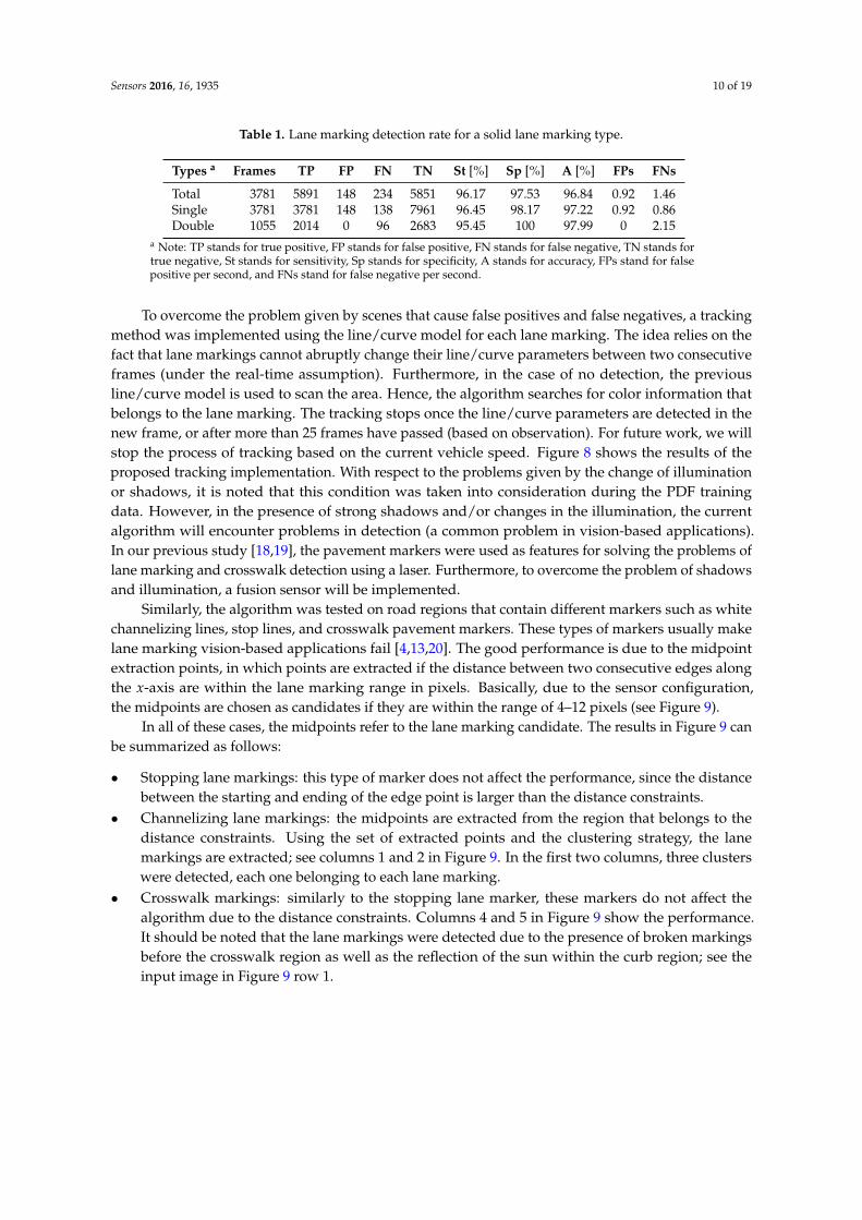
Table 1 shows the result of the proposed algorithm tested in roads with single and double lanemarkings, combining all of them. Although the algorithm was tested in a road with the presence ofshadows, luminance problems, grass, white sand, and deterioration of pavement markings, as well aswithout the presence of shoulders and curbs, the results show good performance.

Sensors 2016, 16, 1935 10 of 19

Table 1. Lane marking detection rate for a solid lane marking type.

Types a Frames TP FP FN TN St [%] Sp [%] A [%] FPs FNs

Total 3781 5891 148 234 5851 96.17 97.53 96.84 0.92 1.46Single 3781 3781 148 138 7961 96.45 98.17 97.22 0.92 0.86Double 1055 2014 0 96 2683 95.45 100 97.99 0 2.15

a Note: TP stands for true positive, FP stands for false positive, FN stands for false negative, TN stands fortrue negative, St stands for sensitivity, Sp stands for specificity, A stands for accuracy, FPs stand for falsepositive per second, and FNs stand for false negative per second.

To overcome the problem given by scenes that cause false positives and false negatives, a trackingmethod was implemented using the line/curve model for each lane marking. The idea relies on thefact that lane markings cannot abruptly change their line/curve parameters between two consecutiveframes (under the real-time assumption). Furthermore, in the case of no detection, the previousline/curve model is used to scan the area. Hence, the algorithm searches for color information thatbelongs to the lane marking. The tracking stops once the line/curve parameters are detected in thenew frame, or after more than 25 frames have passed (based on observation). For future work, we willstop the process of tracking based on the current vehicle speed. Figure 8 shows the results of theproposed tracking implementation. With respect to the problems given by the change of illuminationor shadows, it is noted that this condition was taken into consideration during the PDF trainingdata. However, in the presence of strong shadows and/or changes in the illumination, the currentalgorithm will encounter problems in detection (a common problem in vision-based applications).In our previous study [18,19], the pavement markers were used as features for solving the problems oflane marking and crosswalk detection using a laser. Furthermore, to overcome the problem of shadowsand illumination, a fusion sensor will be implemented.

Similarly, the algorithm was tested on road regions that contain different markers such as whitechannelizing lines, stop lines, and crosswalk pavement markers. These types of markers usually makelane marking vision-based applications fail [4,13,20]. The good performance is due to the midpointextraction points, in which points are extracted if the distance between two consecutive edges alongthe x-axis are within the lane marking range in pixels. Basically, due to the sensor configuration,the midpoints are chosen as candidates if they are within the range of 4–12 pixels (see Figure 9).

In all of these cases, the midpoints refer to the lane marking candidate. The results in Figure 9 canbe summarized as follows:

• Stopping lane markings: this type of marker does not affect the performance, since the distancebetween the starting and ending of the edge point is larger than the distance constraints.

• Channelizing lane markings: the midpoints are extracted from the region that belongs to thedistance constraints. Using the set of extracted points and the clustering strategy, the lanemarkings are extracted; see columns 1 and 2 in Figure 9. In the first two columns, three clusterswere detected, each one belonging to each lane marking.

• Crosswalk markings: similarly to the stopping lane marker, these markers do not affect thealgorithm due to the distance constraints. Columns 4 and 5 in Figure 9 show the performance.It should be noted that the lane markings were detected due to the presence of broken markingsbefore the crosswalk region as well as the reflection of the sun within the curb region; see theinput image in Figure 9 row 1.

Sensors 2016, 16, 1935 11 of 19

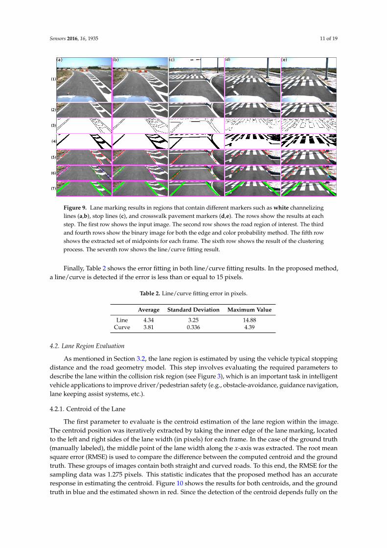
Figure 9. Lane marking results in regions that contain different markers such as white channelizinglines (a,b), stop lines (c), and crosswalk pavement markers (d,e). The rows show the results at eachstep. The first row shows the input image. The second row shows the road region of interest. The thirdand fourth rows show the binary image for both the edge and color probability method. The fifth rowshows the extracted set of midpoints for each frame. The sixth row shows the result of the clusteringprocess. The seventh row shows the line/curve fitting result.

Finally, Table 2 shows the error fitting in both line/curve fitting results. In the proposed method,a line/curve is detected if the error is less than or equal to 15 pixels.

Table 2. Line/curve fitting error in pixels.

Average Standard Deviation Maximum Value

Line 4.34 3.25 14.88Curve 3.81 0.336 4.39

4.2. Lane Region Evaluation

As mentioned in Section 3.2, the lane region is estimated by using the vehicle typical stoppingdistance and the road geometry model. This step involves evaluating the required parameters todescribe the lane within the collision risk region (see Figure 3), which is an important task in intelligentvehicle applications to improve driver/pedestrian safety (e.g., obstacle-avoidance, guidance navigation,lane keeping assist systems, etc.).

4.2.1. Centroid of the Lane

The first parameter to evaluate is the centroid estimation of the lane region within the image.The centroid position was iteratively extracted by taking the inner edge of the lane marking, locatedto the left and right sides of the lane width (in pixels) for each frame. In the case of the ground truth(manually labeled), the middle point of the lane width along the x-axis was extracted. The root meansquare error (RMSE) is used to compare the difference between the computed centroid and the groundtruth. These groups of images contain both straight and curved roads. To this end, the RMSE for thesampling data was 1.275 pixels. This statistic indicates that the proposed method has an accurateresponse in estimating the centroid. Figure 10 shows the results for both centroids, and the groundtruth in blue and the estimated shown in red. Since the detection of the centroid depends fully on the

Sensors 2016, 16, 1935 12 of 19

lane marking detection, the 1.275 RMSE value indicates the feasibility of the proposed lane markingdetection strategy for intelligent vehicle applications.

Figure 10. Centroid evaluation. The figure shows the comparison in pixels between the ground truthcentroid (labeled by hand) and the estimated one. The ground truth is shown in blue while theestimated is shown in red.

4.2.2. Road Geometry Parameters

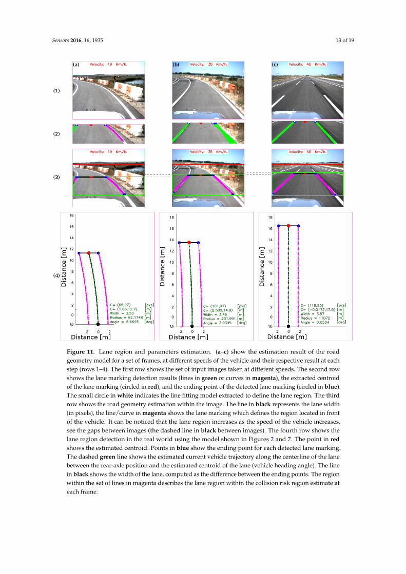
Next, the deflection angle, the chord length, the vehicle heading angle, and the lane width areevaluated. Figure 7 shows the simple circular curve road model used to extract the road parameters.The deflection angle (θ) is the angle formed along the chord length (da). The chord length is thedistance computed between the estimated centroid (circled in red in Figures 7 and 11) and the vehiclerear-axle position (circled in black in Figures 7 and 11). The vehicle heading angle (δ) is the angleformed between the vehicle centerline and the road tangent line. Row 1 in Figure 11 shows a set offrames along straight and curved roads, row 2 shows the result of the lane marking detection, row 3shows the iteratively road geometry model estimation within the input frame, and row 4 shows thelane region detection in the 3D environment at the ground level.

In that sense, the research result in [7] was used to evaluate the proposed method. This was doneas the data for the tested road were collected using both laser and camera sensors simultaneously.As mentioned previously, the data were gathered at the Korea Automobile Testing & Research Institute(KATRI); consequently, extraction of the ground truth for the full path was not possible. This evaluationmethod is used due to the accuracy of laser sensors. Research in [21–23] introduced the use of laserscanning to solve the problem of visual localization within LiDAR maps, extraction of road markingsand lane detection respectively. To this end, Table 3 shows the computed RMSE value between thelaser and camera.

Table 3. Laser-camera root-mean-square error (RMSE) evaluation.

Deflection Angle [◦] Chord Length [m] Vehicle Heading Angle [◦] Lane Width [m]

RMSE 1.28 0.20 0.63 0.40

Figure 12 shows the deflection angle (θ), chord length (da), the vehicle heading angle (δ) andthe lane width estimated for both sensors. Laser and camera results are shown in blue and orangecolors, respectively.

The circles in red show the response of the algorithm when changes in the illumination due tosunlight are presented. Instead of developing an algorithm to solve this problem due to strong sunlight(which increases the computing time), a merging strategy based on laser-vision will be proposed.However, further strategies will be implemented in order to extract the ground truth by adding aposition sensor within the vehicle steering column.

Sensors 2016, 16, 1935 13 of 19

Figure 11. Lane region and parameters estimation. (a–c) show the estimation result of the roadgeometry model for a set of frames, at different speeds of the vehicle and their respective result at eachstep (rows 1–4). The first row shows the set of input images taken at different speeds. The second rowshows the lane marking detection results (lines in green or curves in magenta), the extracted centroidof the lane marking (circled in red), and the ending point of the detected lane marking (circled in blue).The small circle in white indicates the line fitting model extracted to define the lane region. The thirdrow shows the road geometry estimation within the image. The line in black represents the lane width(in pixels), the line/curve in magenta shows the lane marking which defines the region located in frontof the vehicle. It can be noticed that the lane region increases as the speed of the vehicle increases,see the gaps between images (the dashed line in black between images). The fourth row shows thelane region detection in the real world using the model shown in Figures 2 and 7. The point in redshows the estimated centroid. Points in blue show the ending point for each detected lane marking.The dashed green line shows the estimated current vehicle trajectory along the centerline of the lanebetween the rear-axle position and the estimated centroid of the lane (vehicle heading angle). The linein black shows the width of the lane, computed as the difference between the ending points. The regionwithin the set of lines in magenta describes the lane region within the collision risk region estimate ateach frame.

Sensors 2016, 16, 1935 14 of 19

Figure 12. Road parameters evaluation using laser and camera, laser data in blue color while cameradata is in orange color. (a) shows the deflection angle comparison; (b) illustrates the chord lengthcomparison; (c) shows the vehicle heading angle; and (d) shows the lane width comparison. Circles inred shows the computed error due to abrupt change in illumination.

4.3. Comparative Analysis

The proposed method is compared with the latest research. It should be noted that the informationin the tables is related to the best performance results in each study. Additionally, the researchersproposed different strategies to solve the problem, making it difficult to compare results.

Table 4 shows the research results given in [4,5,13,24]. All of these approaches show goodperformance—over a 90% detection rate. However, it should be emphasized that the number of framesused to test their algorithm could affect the results. To test the proposed algorithm, 3781 frameswere used, while Mammeri et al. used 912 frames and Du et al. used 350 for the quantitativecomparison from a total of 2000 frames. Jung et al. mentioned that they recorded road video forthe total time of 1 h and 40 min; however, they do not indicate the number of frames used in theirbest performance. Guo et al. used a set of 2132 frames in their best performance. On the other hand,the road environment, weather condition, and night or day conditions also affect the measurement.To test all of these algorithms, urban roads were used. However, it should be noted that the datasetused to test the proposed method contains barriers, bushes, shadows, spilled markers, and sand the

Sensors 2016, 16, 1935 15 of 19

along the lane marking, as well as different types of markers (see Figure 9), which increases the degreeof difficulty at the moment of detection. To this end, authors in [4,5,13] show a better performancethan the proposed method. In the case of [24], our proposed method shows better performance.

Table 4. Comparison of different techniques in drivable region detection.

Authors a Frame No. DR [%] FDR [%] PT [ms] DA [m]

Proposed method 3781 96.17 2.47 28.30 0.77Mammeri et al. [4] 912 100.00 3.60 �32.31 ** �0.90

Du et al. [13] 350 98.50 2.20 120.04 3.33Jung et al. [5] N/D 98.31 N/D 116.82 3.24Guo et al. [24] 2132 94.79 7.77 40.00 1.10

a Note: DR stands for detection rate, FDR stands for false detection rate, PT stands for processing time,N/D stands for no data, and DA stands for data acquisition at assumed speed of 100 km/h. ** Authors donot discuss information regarding the processing time. Consequently as the information relates to the edgesegmentation results (Table 2 in [4]).

Comparing these algorithms in the presence of different marker types (channeling lines, stop lines,crosswalk), the presented strategy shows a robust response (see Figure 9). Mammeri et al. indicatedthat their algorithm in cross-roads will encounter some problems in the detection of lane markings.Authors refer to the case where crosswalk markings were recognized as lane markings (Figure 12cin [4]). Du et al. mentioned that their algorithm does not work properly in some regions (see Figure 27b,zebra crossing or crosswalk, in [13]). Jung et al. and Guo et al. did not show results related to thementioned marker type regions. Mostly, the given errors are related to the edge extraction step. In otherwords, the edges are used as a feature without taking into consideration the lane marking width,reflecting the use of the edge (from crosswalks or traffic signs), or road markers (such as arrows or text)as a feature. On the contrary, the presented idea takes the size of the lane marking into consideration,reducing the error given by markers of a different type. The strategy presented in this approach showsa better performance in terms of computing time, which is crucial for real-time applications. The dataacquisition interval for each algorithm at an assumed vehicle speed of 100 km/h is shown in thefifth column of Table 4. It can be seen that the proposed algorithm can gather data approximatelyevery 0.8 m between frames.

The computing time improvement in this approach is related to the factors described below.The method efficiently extracts the bounded region of interest within the frame. The ROI in this methodis dynamic and vehicle speed-dependent in a range of (256,(68–105)) pixels in size for speeds in a rangeof [0–100] km/h. In contrast, the latest research using different strategies is relatively time-consuming.For example, the authors in [4] resized the image to 640 × 240 prior to the implementation of theirapproach. Researchers in [13] used the bottommost part of the input image in other words, an imagesize of 640 × 240. Authors in [24] used an image of dimensions 856 × 240, while researchers in [5] useda spatiotemporal image strategy in which processing time should be affected by the camera frame rate.On the other hand, the RANSAC algorithm is applied if and only if the line fitting is insufficient todefinitively model the lane marking within the already defined cluster (see Figure 5, sixth row). This isbecause it was statistically observed that a robust linear fit can be found 95% of time. Consequently,the time-consuming RANSAC algorithm is only used in rare events when it is absolutely necessary fordiscrimination. However, it should be noted that for the case of tight left and right turns, RANSACplays an important role. For example, in [13], authors used simultaneous line/hyperbola road models,which can degrade the algorithm response time. Guo et al. used the RANSAC algorithm along withthe least square method. Although the authors detect left and right markings independently, thenumber of points within the pool and the number of iterations will affect the lane marking detectionresults. Finally, instead of repetitively performing color probability computation during runtime tocompute the metric according to the RGB and S channels, a look-up table was created for each colorchannel according to their respective PDF. The processing time information is shown in Tables 5 and 6.

Sensors 2016, 16, 1935 16 of 19

Table 5. Computational time for each task in milliseconds.

Distance ROI a Color Edge Mid-Points Clustering Fitting Heading Total

0.0407 0.0807 5.8629 6.2400 0.7989 11.788 2.4640 1.0269 28.3021a Note: ROI stands for region of interest extraction.

Table 6. Computing time in milliseconds.

Total Standard Deviation Max. Time

28.3021 7.003 48.99

In order to verify the reliability of the proposed lane marking detection, the Caltech LanesDataset [9] was used to test the algorithm. The results are shown in Figure 13. It should be notedthe difference in both sensor setup as well as field of view of the camera. In the proposed method,the lane ahead of the vehicle is mostly covered within the image, while the Caltech data set coversa larger area. Although the settings in the algorithm were not adjusted, the results showed a goodresponse in the presence of crosswalk areas, arrows, as well as stop lines (Figure 13a,b, respectively).With respect to the traffic signs on the road, the algorithm failed in regions where the width of thesigns was within the distance threshold used in our method to differentiate lane marking (see lines inmagenta in Figure 13c). On the other hand, it was mostly double lane markings were not correctlydetected due to the clustering process. This problem happened because the distance between twolane markings was not enough for the method to correctly separate them. As a consequence, bothlane markings were labeled as the same group (see circles in magenta along the double yellow lanemarking in Figure 13d). Then, the next step (line/curve fitting model) rejected the cluster as a lanemarking since the sum of the error for both line and curve models was greater than the proposedthreshold. Similarly, broken lane markings in some cases were not detected due to the number ofextracted midpoints. In the proposed method, due to the sensor setup and the field of view, thealgorithm considered a lane marking candidate if at least five midpoints were extracted. In the Caltechdataset, in some cases, three midpoints define a broken lane marking. Similarly, lane markings locatedat both sides of the laser (near the curbs) were not detected because PDF training data does notconsider the pixels belonging to lane marking. To this end, the performance of the proposed algorithmusing the Caltech data set is described as follows: specificity of 0.64, sensitivity of 0.95, accuracy 0.79,false positive per second rate of 0.93, and false negative per second rate of 4.64 at processing time of12.13 ms. The program was built in C++ and compiled in Ubuntu 16.04 using an Intel Core i7-4770MQ,2.40 GHz, with 8 GB of RAM, GeForce GT 750M/PCIe/SSE2. In the current implementation, the colorpixel detection is implemented in CUDA (Compute Unified Device Architecture). The encounteredproblems will be solved in the current ongoing laser-camera hybrid method.

Finally, it should be noted that the current algorithm was not tested under environmentalconditions such as rainfall, foggy weather or nighttime. In order to overcome this problem, additionalimprovement will be done by analyzing the reflectance of pavement-marking under these conditions.In the case of camera sensors, the idea will be focused on the approach of enhancing visibility [25,26].In the case of laser sensors, the analysis will be based on the surface patterns characteristic of the roadin the presence of rain water [27] or fog [28]. Research in [7] showed that, in the case of nighttime,the laser demonstrates good performance.

Sensors 2016, 16, 1935 17 of 19

Figure 13. Lane marking evaluation using Caltech dataset. (a) shows the result of the proposed methodin the presence of crosswalk areas; (b) shows the result for the case of stop lines and arrow; (c) showsthe result of the wrong detection due to the text on the road; and (d) shows the error in detection givenby double lane marking. It happens because of the clustering label both on the same cluster, due to thegap between the lane marking.

5. Conclusions

In this paper, a vision based real-time lane marking, lane understanding application was presentedfor use in intelligent vehicles. The aim of this paper has been three-fold:

• To introduce an automated method for extracting the region of interest based on the relationshipbetween the vehicle speed and the typical stopping distance within the image. As a result, theimage is sectioned into three regions: information above the horizon, a zero collision risk, and acollision risk region.

• To propose a real-time lane marking detection strategy combining edge and color features, whichuses the probability that the extracted features define a lane marking, as well as a hierarchicalfitting model. As a result, the method is able to detect lane markings with an accuracy of 96.84% atan average processing time of 28.30 ms, for a speed range of [5–45] km/h. Similarly, the algorithmsolves the problem given by traffic marking signal types such as channelizing lines, stop lines,crosswalks, and arrows.

• To estimate the lane region and the vehicle heading angle by using the road geometry model andthe lane centroid information.

Although a classification method based on a probability density function was used in order toimprove the response in the presence of strong shadows or changes in illumination (which takes intoconsideration yellow, white and lane marking with shadows), there will be future improvements.These improvements will be made by developing a laser-camera hybrid method; the results of theongoing process are shown in [29]. Similarly, the proposed method will be improved by taking differentenvironmental conditions into consideration.

Acknowledgments: This work was supported by the National Research Foundation of Korea (NRF) Grant fundedby the Korean Government (2016R1D1A1A02937579).

Sensors 2016, 16, 1935 18 of 19

Author Contributions: D. Cáceres H. and K. H. Jo proposed the idea and wrote the paper. D. Cáceres H. andL. Kurnianggoro worked on the platform design and the data gathering algorithm based on laser and camera.D. Cáceres H. and A. Filonenko worked on the algorithm implementation. K. H. Jo supervised the research work.

Conflicts of Interest: The authors declare no conflict of interest.

References

1. Sun, T.Y.; Tsai, S.J.; Chan, V. HSI color model based lane-marking detection. In Proceedings of the 2006 IEEEIntelligent Transportation Systems Conference, Toronto, ON, Canada, 17–20 September 2006; pp. 1168–1172.

2. Tran, T.T.; Bae, C.S.; Kim, Y.N.; Cho, H.M.; Cho, S.B. An Adaptive Method for Lane Marking Detection Basedon HSI Color Model. In Proceedings of the 6th International Conference on Intelligent Computing AdvancedIntelligent Computing Theories and Applications, Changsha, China, 18–21 August 2010; pp. 304–311.

3. Du, X.; Tan, K.K. Comprehensive and Practical Vision System for Self-Driving Vehicle Lane-LevelLocalization. IEEE Trans. Image Process. 2016, 25, 2075–2088.

4. Mammeri, A.; Boukerche, A.; Tang, Z. A real-time lane marking localization, tracking and communicationsystem. Comput. Commun. 2016, 73, 132–143.

5. Jung, S.; Youn, J.; Sull, S. Efficient Lane Detection Based on Spatiotemporal Images. IEEE Trans. Intell.Transp. Syst. 2016, 17, 289–295.

6. James, A.P.; Al-Jumeily, D.; Thampi, S.M.; John, N.; Anusha, B.; Kutty, K. A reliable method for detecting roadregions from a single image based on color distribution and vanishing point location. Procedia Comput. Sci.2015, 58, 2–9.

7. Cáceres H.D.; Filonenko, A.; Seo, D.; Jo, K.H. Laser scanner based heading angle and distance estimation.In Proceedings of the 2015 IEEE International Conference on Industrial Technology, Seville, Spain,17–19 March 2015; pp. 1718–1722.

8. Cáceres H.D.; Seo, D.; Jo, K.H. Robust lane marking detection based on multi-feature fusion. In Proceedingsof the 9th International Conference on Human System Interaction (HSI), Portsmouth, UK, 6–8 July 2016;pp. 423–428.

9. Aly, M. Real time detection of lane markers in urban streets. In Proceedings of the 2008 IEEE IntelligentVehicles Symposium, Eindhoven, The Netherlands, 4–6 June 2008; pp. 7–12.

10. Li, Q.; Zheng, N.; Cheng, H. Springrobot: A prototype autonomous vehicle and its algorithms for lanedetection. IEEE Trans. Intell. Transp. Syst. 2004, 5, 300–308.

11. Otsu, N. A Threshold Selection Method from Gray-Level Histograms. IEEE Trans. Syst. Man Cybern. 1979,9, 62–66.

12. Canny, J. A Computational Approach to Edge Detection. IEEE Trans. Pattern Anal. Mach. Intell. 1986,PAMI-8, 679–698.

13. Du, X.; Tan, K.K. Vision-based approach towards lane line detection and vehicle localization. Mach. Vis. Appl.2016, 27, 175–191.

14. Lu, M.C.; Hsu, C.C.; Lu, Y.Y. Image-Based System for Measuring Objects on an Oblique Plane and ItsApplications in 2-D Localization. IEEE Sens. J. 2012, 12, 2249–2261.

15. Lu, M.C.; Hsu, C.C.; Lu, Y.Y. Distance and angle measurement of distant objects on an oblique plane basedon pixel variation of CCD image. In Proceedings of the 2010 IEEE Instrumentation and MeasurementTechnology Conference, Austin, TX, USA, 3–6 May 2010; pp. 318–322.

16. Pauly, N.; Rafla, N.I. An automated embedded computer vision system for object measurement.In Proceedings of the 2013 IEEE 56th International Midwest Symposium on Circuits and Systems, Columbus,OH, USA, 4–7 August 2013; pp. 1108–1111.

17. Fernandes, J.C.A.; Neves, J.A.B.C. Angle Invariance for Distance Measurements Using a Single Camera.In Proceedings of the 2006 IEEE International Symposium on Industrial Electronics, Montreal, QC, Canada,9–13 July 2006; pp. 676–680.

18. Hernández, D.C.; Filonenko, A.; Seo, D.; Jo, K.H. Lane marking recognition based on laser scanning.In Proceedings of the 2015 IEEE 24th International Symposium on Industrial Electronics, Búzios, Brazil,3–5 June 2015; pp. 962–965.

Sensors 2016, 16, 1935 19 of 19

19. Hernández, D.C.; Filonenko, A.; Seo, D.; Jo, K.H. Crosswalk detection based on laser scanning from movingvehicle. In Proceedings of the 2015 IEEE 13th International Conference on Industrial Informatics, Cambridge,UK, 22–24 July 2015; pp. 1515–1519.

20. Tran, T.T.; Cho, H.M.; Cho, S.B. A robust method for detecting lane boundary in challenging scenes.Inf. Technol. 2011, 10, 2300–2307.

21. Wolcott, R.; Eustice, R. Visual localization within LIDAR maps for automated urban driving. In Proceedingsof the 2014 IEEE/RSJ International Conference on Intelligent Robots and Systems, Chicago, IL, USA,14–18 September 2014; pp. 176–183.

22. Guan, H.; Li, J.; Yu, Y.; Chapman, M.; Wang, C. Automated Road Information Extraction From Mobile LaserScanning Data. IEEE Trans. Intell. Transp. Syst. 2015, 16, 194–205.

23. Guan, H.; Li, J.; Yu, Y.; Wang, C.; Chapman, M.; Yang, B. Using mobile laser scanning data for automatedextraction of road markings. ISPRS J. Photogramm. Remote Sens. 2014, 87, 93–107.

24. Guo, J.; Wei, Z.; Miao, D. Lane Detection Method Based on Improved RANSAC Algorithm. In Proceedings ofthe 2015 IEEE Twelfth International Symposium on Autonomous Decentralized Systems, Taichung, Taiwan,25–27 March 2015; pp. 285–288.

25. Zhang, Y.Q.; Ding, Y.; Xiao, J.S.; Liu, J.; Guo, Z. Visibility enhancement using an image filtering approach.EURASIP J. Adv. Signal Process. 2012, 2012, 220.

26. Huang, S.C.; Chen, B.H.; Cheng, Y.J. An Efficient Visibility Enhancement Algorithm for Road ScenesCaptured by Intelligent Transportation Systems. IEEE Trans. Intell. Transp. Syst. 2014, 15, 2321–2332.

27. Lantieri, C.; Lamperti, R.and Simone, A.D.G. Mobile Laser Scanning System for Assessment of the RainwaterRunoff and Drainage Conditions on Road Pavements. Int. J. Pavement Res. Technol. 2015, 8, 1–9.

28. Sallis, P.; Dannheim, C.; Icking, C.; Maeder, M. Air Pollution and Fog Detection through Vehicular Sensors.In Proceedings of the 2014 8th Asia Modelling Symposium, Taiwan, 23–25 September 2014; pp. 181–186.

29. Hybrid Lane Detection Results Using Camera and Laser Sensors. Available online: http://islab.ulsan.ac.kr/supplementary/lane_detection/lane_detection_result_camera_laser.avi (accessed on 15 November 2016).

c© 2016 by the authors; licensee MDPI, Basel, Switzerland. This article is an open accessarticle distributed under the terms and conditions of the Creative Commons Attribution(CC-BY) license (http://creativecommons.org/licenses/by/4.0/).