Embed Size (px)
Citation preview
University of Tennessee, Knoxville University of Tennessee, Knoxville
TRACE: Tennessee Research and Creative TRACE: Tennessee Research and Creative
Exchange Exchange
Masters Theses Graduate School
8-2012
Real-Time Mobile Stereo Vision Real-Time Mobile Stereo Vision
Bryan Hale Bodkin [email protected]
Follow this and additional works at: https://trace.tennessee.edu/utk_gradthes
Part of the Artificial Intelligence and Robotics Commons, Robotics Commons, and the Software
Engineering Commons
Recommended Citation Recommended Citation Bodkin, Bryan Hale, "Real-Time Mobile Stereo Vision. " Master's Thesis, University of Tennessee, 2012. https://trace.tennessee.edu/utk_gradthes/1313
This Thesis is brought to you for free and open access by the Graduate School at TRACE: Tennessee Research and Creative Exchange. It has been accepted for inclusion in Masters Theses by an authorized administrator of TRACE: Tennessee Research and Creative Exchange. For more information, please contact [email protected].

To the Graduate Council:
I am submitting herewith a thesis written by Bryan Hale Bodkin entitled "Real-Time Mobile
Stereo Vision." I have examined the final electronic copy of this thesis for form and content and
recommend that it be accepted in partial fulfillment of the requirements for the degree of
Master of Science, with a major in Computer Engineering.
Hairong Qi, Major Professor
We have read this thesis and recommend its acceptance:
Qing Cao, Jens Gregor
Accepted for the Council:
Carolyn R. Hodges
Vice Provost and Dean of the Graduate School
(Original signatures are on file with official student records.)

Real-Time Mobile Stereo Vision
A Thesis Presented for
The Master of Science
Degree
The University of Tennessee, Knoxville
Bryan Hale Bodkin
August 2012

c© by Bryan Hale Bodkin, 2012
All Rights Reserved.
ii

Acknowledgments
I would like to thank Dr. Qi for giving me the time and resources to pursue my
research interests. I would also like to thank Dr. Cao and Dr Gregor for serving on
my committee.
iii
Abstract
Computer stereo vision is used to extract depth information from two aligned cameras
and there are a number of hardware and software solutions to solve the stereo
correspondence problem. However few solutions are available for inexpensive mobile
platforms where power and hardware are major limitations. This thesis proposes a
method that competes with an existing OpenCV stereo correspondence method in
speed and quality, and is able to run on generic multi core CPUs.
iv
Contents
List of Tables viii
List of Figures ix
1 Introduction 1
1.1 Introduction to Stereo Vision . . . . . . . . . . . . . . . . . . . . . . 2
1.2 Reference and Target . . . . . . . . . . . . . . . . . . . . . . . . . . . 3
1.3 Camera Alignment . . . . . . . . . . . . . . . . . . . . . . . . . . . . 3
2 Stereo Correspondence Methods 5
2.1 Pixel based Methods . . . . . . . . . . . . . . . . . . . . . . . . . . . 5
2.2 Area-based Methods . . . . . . . . . . . . . . . . . . . . . . . . . . . 6
2.3 Feature-based Methods . . . . . . . . . . . . . . . . . . . . . . . . . . 6
2.4 Cost Matching Functions . . . . . . . . . . . . . . . . . . . . . . . . . 7
2.5 Common Cost Matching Functions . . . . . . . . . . . . . . . . . . . 7
2.6 Correspondence Functions . . . . . . . . . . . . . . . . . . . . . . . . 8
3 Block Matching 10
3.1 Core Technologies . . . . . . . . . . . . . . . . . . . . . . . . . . . . . 10
3.2 OpenCVs Block Matching Function . . . . . . . . . . . . . . . . . . . 11
3.3 Naive Stereo Matching Function . . . . . . . . . . . . . . . . . . . . . 11
3.4 Test Hardware . . . . . . . . . . . . . . . . . . . . . . . . . . . . . . . 11
3.5 Test Stereo Images . . . . . . . . . . . . . . . . . . . . . . . . . . . . 12
v
3.6 Naive Stereo Correspondence and OpenCV BM Comparison . . . . . 12
3.7 Sliding Window Technique . . . . . . . . . . . . . . . . . . . . . . . . 13
3.7.1 Intermediate Data Structures for the Sliding Window Technique 14
3.7.2 The Four Main Processes . . . . . . . . . . . . . . . . . . . . . 14
3.7.3 Sliding Window Performance . . . . . . . . . . . . . . . . . . 15
3.8 Improvements with SIMD Instructions . . . . . . . . . . . . . . . . . 15
3.8.1 Intel SSE overview . . . . . . . . . . . . . . . . . . . . . . . . 17
3.8.2 SSE with C++ . . . . . . . . . . . . . . . . . . . . . . . . . . 17
3.8.3 Changes in Intermediate Data Structures for SSE . . . . . . . 19
3.8.4 SSE Intrinsics Overview . . . . . . . . . . . . . . . . . . . . . 19
3.8.5 SSE Row Difference . . . . . . . . . . . . . . . . . . . . . . . . 19
3.8.6 SSE Row Summing Window . . . . . . . . . . . . . . . . . . . 22
3.8.7 SSE Column Summing Window . . . . . . . . . . . . . . . . . 22
3.8.8 SSE Winner Take All . . . . . . . . . . . . . . . . . . . . . . . 22
3.8.9 SSE with Sliding Window Performance . . . . . . . . . . . . . 24
3.9 Improving performance with Parallelism . . . . . . . . . . . . . . . . 25
3.9.1 Dividing the Data . . . . . . . . . . . . . . . . . . . . . . . . . 25
3.9.2 Parallelism Performance . . . . . . . . . . . . . . . . . . . . . 26
4 Applying Stereo Method to Real Cameras 28
4.1 Calibration . . . . . . . . . . . . . . . . . . . . . . . . . . . . . . . . 29
4.1.1 Hardware . . . . . . . . . . . . . . . . . . . . . . . . . . . . . 29
4.1.2 Calibration Procedure . . . . . . . . . . . . . . . . . . . . . . 30
4.2 Real-time Rectification . . . . . . . . . . . . . . . . . . . . . . . . . . 31
4.2.1 Optimized Nearest-Neighbor . . . . . . . . . . . . . . . . . . . 31
4.2.2 Optimized Nearest-Neighbor Performance . . . . . . . . . . . 33
4.3 Complete System . . . . . . . . . . . . . . . . . . . . . . . . . . . . . 34
5 Conclusions and Future Work 37
5.1 Conclusions . . . . . . . . . . . . . . . . . . . . . . . . . . . . . . . . 37
vi

5.2 Future Work . . . . . . . . . . . . . . . . . . . . . . . . . . . . . . . . 37
Bibliography 39
A Listings of Code 43
A.1 Chapter 3 Code . . . . . . . . . . . . . . . . . . . . . . . . . . . . . . 43
A.2 Chapter 4 Code . . . . . . . . . . . . . . . . . . . . . . . . . . . . . . 49
Vita 53
vii
List of Tables
3.1 Naive Stereo Performance . . . . . . . . . . . . . . . . . . . . . . . . 13
3.2 Windowing Stereo Performance . . . . . . . . . . . . . . . . . . . . . 15
3.3 SSE Intrinsic Reference . . . . . . . . . . . . . . . . . . . . . . . . . . 21
3.4 SIMD Stereo Performance . . . . . . . . . . . . . . . . . . . . . . . . 25
3.5 Parallel Stereo Performance . . . . . . . . . . . . . . . . . . . . . . . 27
4.1 Tsai’s Model Estimation Parameters . . . . . . . . . . . . . . . . . . 28
4.2 24-bit Color Remapping . . . . . . . . . . . . . . . . . . . . . . . . . 35
4.3 8-bit Grey Remapping . . . . . . . . . . . . . . . . . . . . . . . . . . 35
viii

List of Figures
1.1 Epiplor Line Structure . . . . . . . . . . . . . . . . . . . . . . . . . . 4
3.1 Tsukuba Data Set . . . . . . . . . . . . . . . . . . . . . . . . . . . . . 12
3.2 Naive Correspondence Comparison . . . . . . . . . . . . . . . . . . . 13
3.3 Intermediate Data Structures . . . . . . . . . . . . . . . . . . . . . . 14
3.4 Intermediate Data Structures . . . . . . . . . . . . . . . . . . . . . . 16
3.5 SSE Register Packing . . . . . . . . . . . . . . . . . . . . . . . . . . . 18
3.6 SSE Array Fitting . . . . . . . . . . . . . . . . . . . . . . . . . . . . 20
3.7 Intermediate Data Structures with Over-fitting . . . . . . . . . . . . . 20
3.8 SSE Row Absolute Difference . . . . . . . . . . . . . . . . . . . . . . 20
3.9 SSE Row Summing Window Process . . . . . . . . . . . . . . . . . . 23
3.10 SSE Column Summing Process . . . . . . . . . . . . . . . . . . . . . 23
3.11 SSE Winner Take All Process . . . . . . . . . . . . . . . . . . . . . . 24
3.12 Parallel Data Division and Recombination . . . . . . . . . . . . . . . 26
3.13 Multi-Threading Performance . . . . . . . . . . . . . . . . . . . . . . 27
4.1 Cameras and Mounting Rig . . . . . . . . . . . . . . . . . . . . . . . 29
4.2 Calebration Images with cvDrawChessboardCorners . . . . . . . . . 32
4.3 Rectified Stereo Image Pair . . . . . . . . . . . . . . . . . . . . . . . 32
4.4 Nearest Neighbor Rectification . . . . . . . . . . . . . . . . . . . . . . 33
4.5 Complete Stereo Imaging Process . . . . . . . . . . . . . . . . . . . . 36
ix
Chapter 1
Introduction
In computer stereo vision, two cameras are placed horizontally from one another and
the difference between the views are used to map the depth of the environment. This
method of depth mapping is in contrast to Light Detection And Ranging (LiDAR).
Stereo vision is cheaper, completely passive, but computationally expensive, while
LiDAR is relatively expensive, requires active laser projection, but requires much less
processing.
This Thesis will focus on the real time general-purpose CPU calculation of
computer stereo vision for a swarm of mobile robots using generic USB webcams.
A number of hardware choices are well suited for the massive parallel computing
potential of stereo vision. But cost and power requirements limit the choices.
Application-Specific Integrated Circuits (ASIC), would be the highest form of
low power and speed, but the astronomical setup cost for manufacturing and
unconfigurable nature of ASICs make them a poor choice.
Consumer level Graphics Processing Units (GPU) are ample with parallel
processing potential and very configurable. GPUs can be purchased for as little as
$80 but still requires a host CPU to run. The largest problem with GPU computing
is the power and cooling requirements, often requiring fifty (50) to one-hundred (100)
1
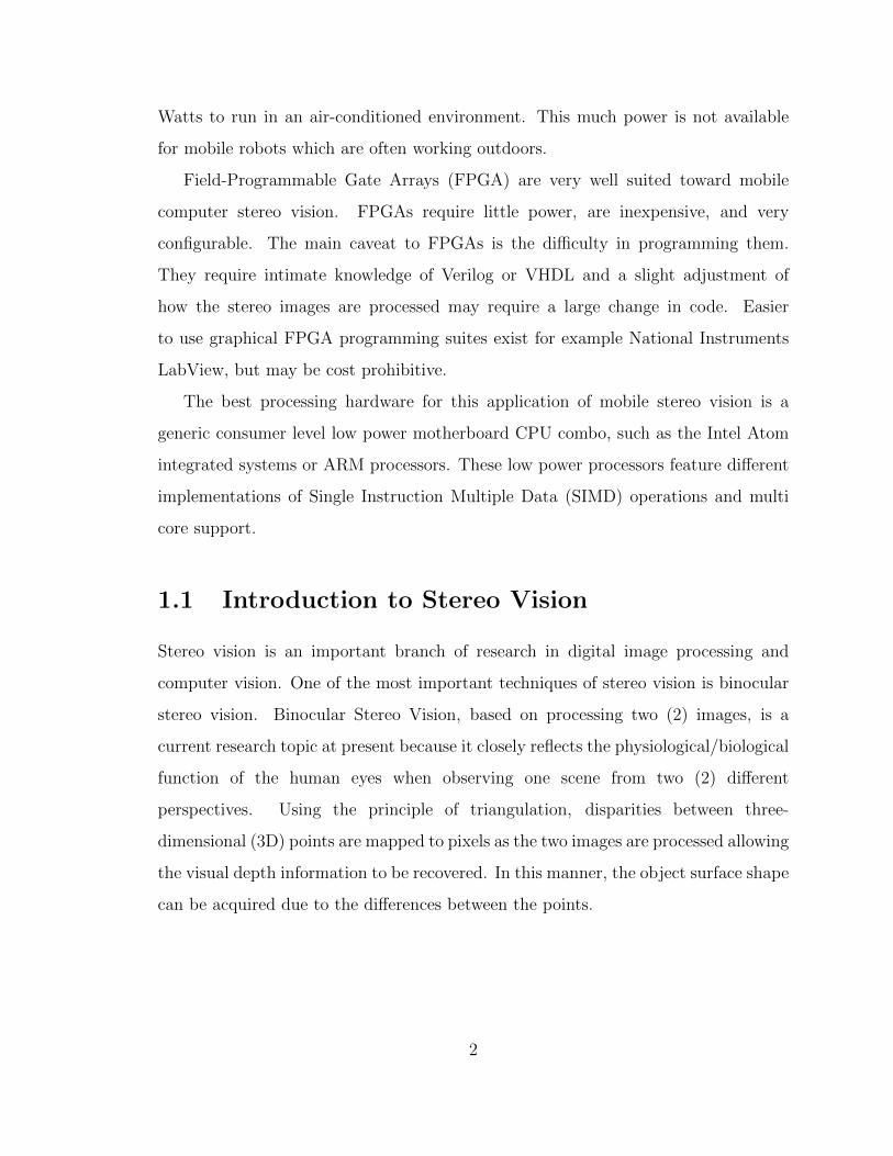
Watts to run in an air-conditioned environment. This much power is not available
for mobile robots which are often working outdoors.
Field-Programmable Gate Arrays (FPGA) are very well suited toward mobile
computer stereo vision. FPGAs require little power, are inexpensive, and very
configurable. The main caveat to FPGAs is the difficulty in programming them.
They require intimate knowledge of Verilog or VHDL and a slight adjustment of
how the stereo images are processed may require a large change in code. Easier
to use graphical FPGA programming suites exist for example National Instruments
LabView, but may be cost prohibitive.
The best processing hardware for this application of mobile stereo vision is a
generic consumer level low power motherboard CPU combo, such as the Intel Atom
integrated systems or ARM processors. These low power processors feature different
implementations of Single Instruction Multiple Data (SIMD) operations and multi
core support.
1.1 Introduction to Stereo Vision
Stereo vision is an important branch of research in digital image processing and
computer vision. One of the most important techniques of stereo vision is binocular
stereo vision. Binocular Stereo Vision, based on processing two (2) images, is a
current research topic at present because it closely reflects the physiological/biological
function of the human eyes when observing one scene from two (2) different
perspectives. Using the principle of triangulation, disparities between three-
dimensional (3D) points are mapped to pixels as the two images are processed allowing
the visual depth information to be recovered. In this manner, the object surface shape
can be acquired due to the differences between the points.
2
1.2 Reference and Target
From the two (2) images, one is declared a reference image and the other is referred
as the target image. For every single pixel in the reference image, the target image
must be searched to find its corresponding location. The distance in pixels between
the final corresponding locations is the disparity. When all pixels in the reference
image have been corresponded to a pixel location in the target image, a complete
dense disparity map is found.
The selection of the reference and target images from the stereo image pair can
be associated to either image. Most often the left stereo image is the reference and
the right is the target image. Some stereo matching techniques may use the left and
right stereo images as both the reference and target images to get better accuracy
and reduce occlusion errors. These methods may take it a step further and generate
a depth map from a point of view between the stereo image camera perspectives.
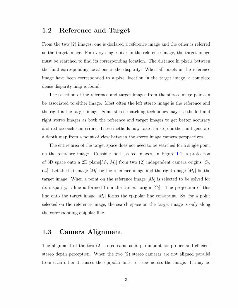
The entire area of the target space does not need to be searched for a single point
on the reference image. Consider both stereo images, in Figure 1.1, a projection
of 3D space onto a 2D plane[Ml, Mr] from two (2) independent camera origins [Cl,
Cr]. Let the left image [Ml] be the reference image and the right image [Mr] be the
target image. When a point on the reference image [Ml] is selected to be solved for
its disparity, a line is formed from the camera origin [Cl]. The projection of this
line onto the target image [Mr] forms the epipolar line constraint. So, for a point
selected on the reference image, the search space on the target image is only along
the corresponding epipolar line.
1.3 Camera Alignment
The alignment of the two (2) stereo cameras is paramount for proper and efficient
stereo depth perception. When the two (2) stereo cameras are not aligned parallel
from each other it causes the epipolar lines to skew across the image. It may be
3
acceptable in some stereo systems to process the images with skewed eplipolar lines,
however for real time systems; it is much more computationally efficient to have the
epipolar lines parallel with one another and row aligned with the image scan lines.
This way, when scanning the line of pixels that make up the epipolar line, the next
pixel in the line is the next place in memory instead of having to refer to a lookup
table.
Figure 1.1: Epiplor Line Structure
4
Chapter 2
Stereo Correspondence Methods
Stereo correspondence is the corner stone of stereo vision. It is the process of matching
areas and or specific locations between the two stereo cameras. Many methods exist
to solve this problem, often trading speed for accuracy or vice versa.
2.1 Pixel based Methods
Pixel-based methods are based on brightness intensity values that compare two (2)
images, pixel by pixel along the epipolar lines and choose a corresponding disparity
that best fits the cost function. Pixel-based methods by themselves are sensitive
to noise but may show finer detail around corners of objects in the stereo image
pair. Two common techniques are used to reduce the noise sensitivity and increase
accuracy of pixel-based methods. One, pre-filters may be used on the stereo image
pair to reduce sources of noise, sacrificing some fine detail Hirschmuller (2007). And
two, global-optimization algorithms can be used to find the best fit for all pixels
across an epipolar line Scharstein (2001). The global-optimization methods are the
most accurate but require the most amount of processing time.
5
2.2 Area-based Methods
Area-based or block matching methods are based on brightness intensity values
aggregated over a local support window between the two (2) comparable images.
The local support window, is convolved between the two (2) stereo images across
the epipolar lines. Common aggregation methods include square window, Gaussian
convolution Scharstein (2001), multi window, and shiftable window techniques Kuk-
Jin (2006).
Area-based methods are less computationally expensive than globally optimized
pixel-based correspondence. However, they are not sensitive to noise and produce
complete dense disparity maps like pixel-based methods. But at the cost of reduced
noise sensitivity, accuracy is lost in high contrast areas of the image pair.
2.3 Feature-based Methods
Feature-based methods use detected feature points to highlight areas of high diversity
in the image pair. Feature points may include edges, lines, regions, and gradient
peaks. By only including feature points with high texture diversity, areas of hard to
match low texture diversity are not matched with another. Since only the feature
points are correlated, the computation cost is greatly reduced. However, a complete
dense disparity map cannot be obtained. Additionally, feature-based methods have
a great immunity to noise.
It should be noted that the feature-based methods are intended to reduce
processing time for stereo matching, so consideration is taken on choosing a feature
extractor that does not consume more computation time than it saves.
6
2.4 Cost Matching Functions
All stereo correspondence algorithms have a way of measuring the similarity of
image pixel locations. Typically, a matching cost is computed at each pixel for
all disparities under consideration. The simplest matching costs assume constant
intensities at matching image locations, but more robust costs model certain
radiometric changes and/or noise. Common pixel-based matching costs include
absolute differences, squared differences, sampling-insensitive absolute differences, or
truncated versions, both on gray and color images. Common window-based matching
costs include the sum of absolute or squared differences (SAD / SSD), normalized
cross correlation (NCC), and rank and census transforms. Some window-based
costs can be implemented efficiently using filter. For example, the rank transform
can be computed using a rank filter followed by absolute differences of the filter
results. Similarly, there are other filters that try to remove bias or gain changes, e.g.,
logarithmic and mean filters. Hirschmuller (2007)
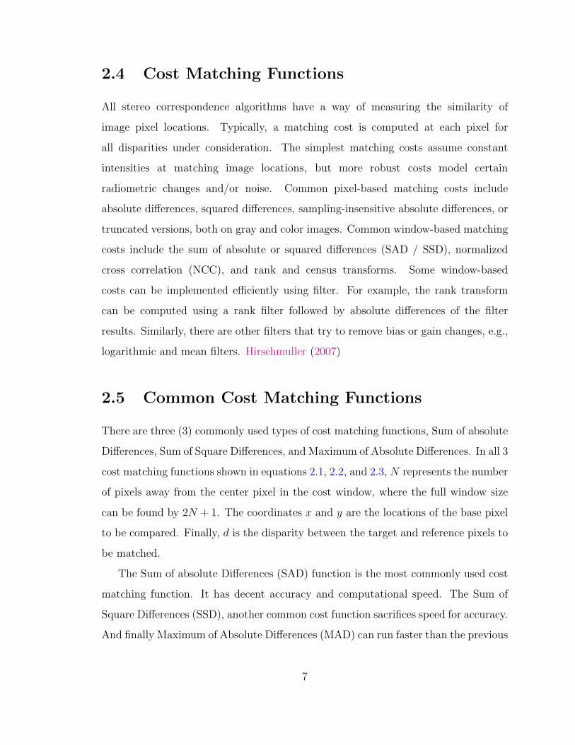
2.5 Common Cost Matching Functions
There are three (3) commonly used types of cost matching functions, Sum of absolute
Differences, Sum of Square Differences, and Maximum of Absolute Differences. In all 3
cost matching functions shown in equations 2.1, 2.2, and 2.3, N represents the number
of pixels away from the center pixel in the cost window, where the full window size
can be found by 2N + 1. The coordinates x and y are the locations of the base pixel
to be compared. Finally, d is the disparity between the target and reference pixels to
be matched.
The Sum of absolute Differences (SAD) function is the most commonly used cost
matching function. It has decent accuracy and computational speed. The Sum of
Square Differences (SSD), another common cost function sacrifices speed for accuracy.
And finally Maximum of Absolute Differences (MAD) can run faster than the previous
7
two methods but is the least accurate. For this thesis, Sum of absolute Differences
will be used.
Sum of Absolute Differences (SAD)
n=N∑n=−N
m=N∑m=−N
∣∣Mln+x,m+y −Mrn+x+d,m+y
∣∣ (2.1)
Sum of Square Differences (SSD)
n=N∑n=−N
m=N∑m=−N
(Mln+x,m+y −Mrn+x+d,m+y
)2(2.2)
Maximum of Absolute Differences (MAD)
max−N≤n≤N [max−N≤m≤N
∣∣Mln+x,m+y −Mrn+x+d,m+y
∣∣] (2.3)
2.6 Correspondence Functions
Correspondence cost functions are used to compare row aligned stereo image pairs to
one another. These cost functions will take a specified pixel location defined by (x,y)
from the left and right images defined by Ml and Mr respectively and compare an area
of pixels. In a naive search, the cost function is cross correlated with every pixel in
the left and right image rows to find the lowest cost pixel pairs. The final disparity is
chosen at the minimum value from the cost matching function. This is also known as
the Winner Take All (WTA) method. Many more advanced correspondence methods
exist that can achieve higher accuracy, but the WTA method is simple and very fast.
To limit the search area, a minimum and maximum disparity is often chosen.
This will help reduce computation time at the expense of eliminating a search-able
depth from the stereo cameras. A small disparity is associated with objects far in the
distance; while larger disparities are very close to the stereo cameras. This thesis’s
8

algorithm grounds the minimum disparity at zero (0) and allows a maximum search-
able disparity to be set.
9
Chapter 3
Block Matching
3.1 Core Technologies
Before delving into stereo vision block matching, a few technologies need to be
addressed for their integral role in this thesis. First, a core part of this thesis uses the
OpenCV(Open source Computer Vision) API (Application Programming Interface).
It is a consolidation of hundreds of computer vision algorithms and provides basic
structures for managing images in C++. This thesis mainly uses OpenCV to acquire
images from cameras, display the images to the screen, and save the images to the
hard drive. OpenCV also provides the competing block matching function this thesis
attempts to improve.
The Second technology that needs to be addressed are Single Instruction Multiple
Data (SIMD) operations. As the acronym implies, it is a way of processing arrays of
data with a single instruction in very few process cycles. Many processor manufactures
support some flavor of SIMD operations and for this thesis, Intel’s Streaming SIMD
Extensions (SSE) will be used.
10
3.2 OpenCVs Block Matching Function
OpenCV uses an existing stereo correspondence block matching function known as
the very fast SAD-based stereo correspondence algorithm. It was written by Kurt
Konolige and utilizes SSE2 instructions. The algorithm supports many parameters
from maximum search-able disparity to the starting disparity value. It also includes a
Sombel pre-filter to help remove noise and texture uniqueness testing. For this thesis,
the Sombel pre-filter and uniqueness testing will not be used to better compare with
this thesis’s algorithm.
3.3 Naive Stereo Matching Function
The first iteration of this thesis’s stereo matching algorithm is a functional but naive
algorithm. The algorithm uses three (3) nested loops to search over the maximum
disparity and the SAD windows, and chooses the pixel disparity with the associated
minimum SAD window. For a given image with N pixels the Big O notation is O(N3).
See C++ code in Appendix A.1
3.4 Test Hardware
For performance comparisons two (2) computers are used to run the stereo algorithms.
First a desktop computer with a 2.3 GHz Intel Core 2 Quad processor (Q8200) with
8GBs of memory. Second a Dell laptop with a quad core Intel i7 processor (i7-720Q)
with a clock speed of 1.6Ghz with 4GBs of memory. Both computers are running
Windows 7.
11
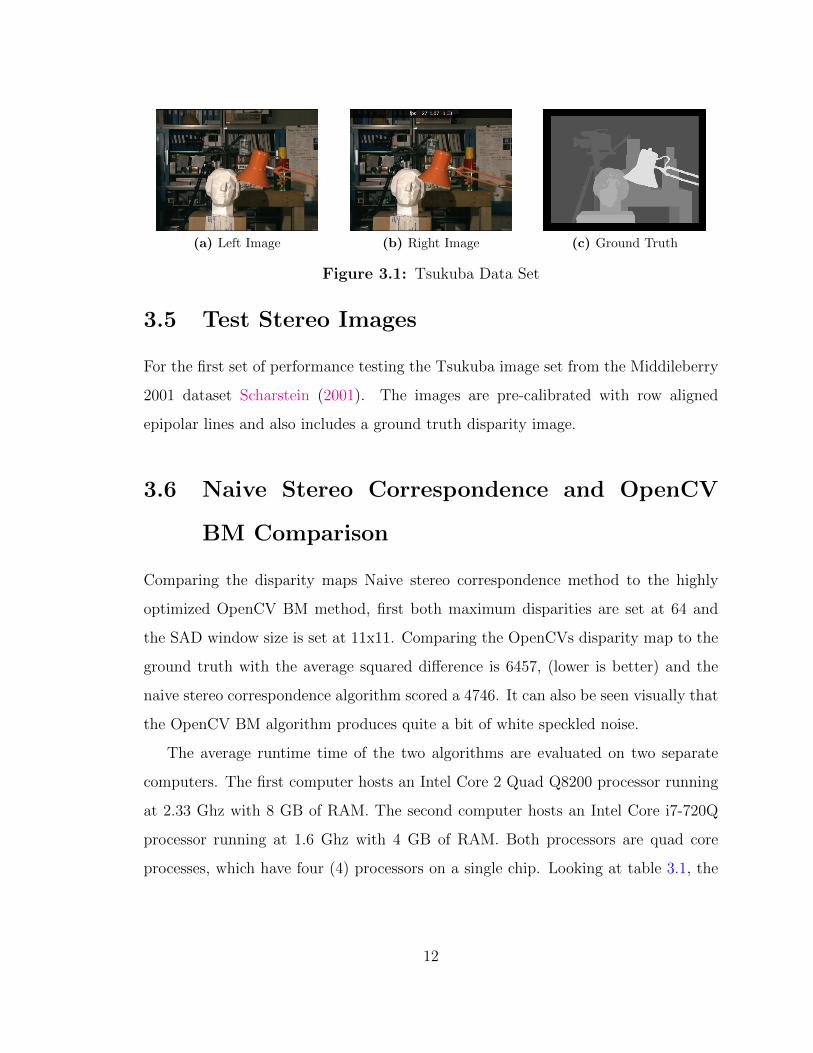
(a) Left Image (b) Right Image (c) Ground Truth
Figure 3.1: Tsukuba Data Set
3.5 Test Stereo Images
For the first set of performance testing the Tsukuba image set from the Middileberry
2001 dataset Scharstein (2001). The images are pre-calibrated with row aligned
epipolar lines and also includes a ground truth disparity image.
3.6 Naive Stereo Correspondence and OpenCV
BM Comparison
Comparing the disparity maps Naive stereo correspondence method to the highly
optimized OpenCV BM method, first both maximum disparities are set at 64 and
the SAD window size is set at 11x11. Comparing the OpenCVs disparity map to the
ground truth with the average squared difference is 6457, (lower is better) and the
naive stereo correspondence algorithm scored a 4746. It can also be seen visually that
the OpenCV BM algorithm produces quite a bit of white speckled noise.
The average runtime time of the two algorithms are evaluated on two separate
computers. The first computer hosts an Intel Core 2 Quad Q8200 processor running
at 2.33 Ghz with 8 GB of RAM. The second computer hosts an Intel Core i7-720Q
processor running at 1.6 Ghz with 4 GB of RAM. Both processors are quad core
processes, which have four (4) processors on a single chip. Looking at table 3.1, the
12
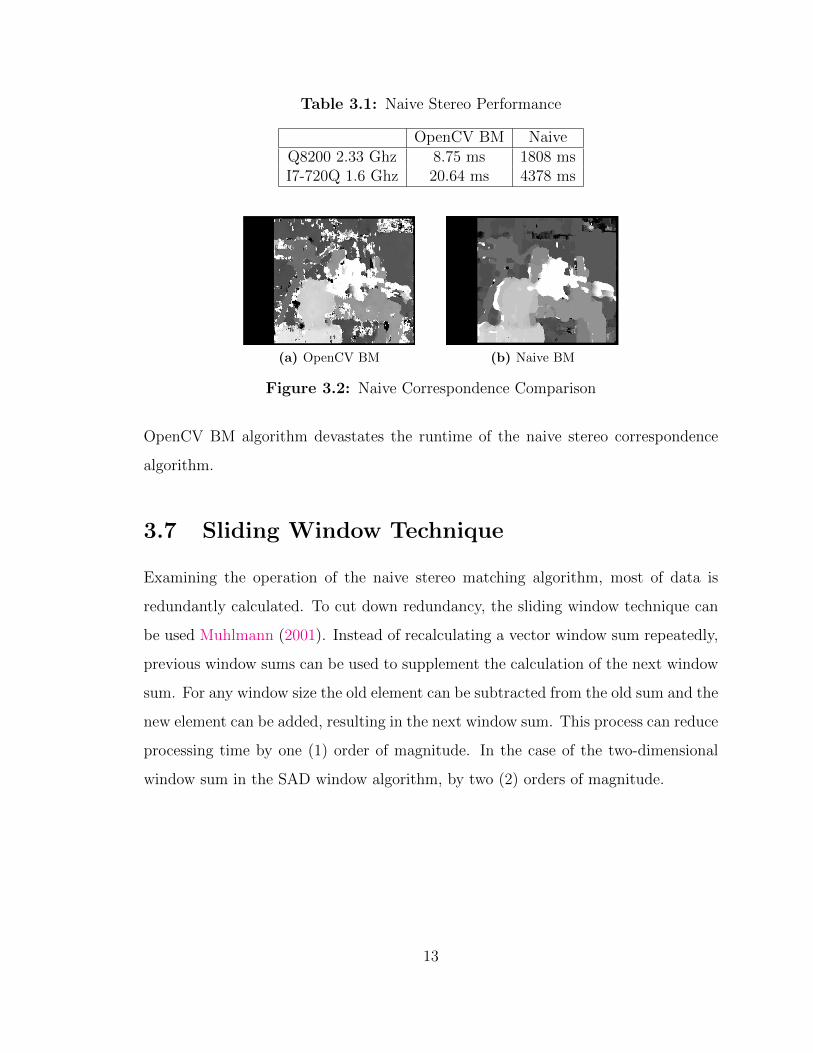
Table 3.1: Naive Stereo Performance
OpenCV BM NaiveQ8200 2.33 Ghz 8.75 ms 1808 msI7-720Q 1.6 Ghz 20.64 ms 4378 ms
(a) OpenCV BM (b) Naive BM
Figure 3.2: Naive Correspondence Comparison
OpenCV BM algorithm devastates the runtime of the naive stereo correspondence
algorithm.
3.7 Sliding Window Technique
Examining the operation of the naive stereo matching algorithm, most of data is
redundantly calculated. To cut down redundancy, the sliding window technique can
be used Muhlmann (2001). Instead of recalculating a vector window sum repeatedly,
previous window sums can be used to supplement the calculation of the next window
sum. For any window size the old element can be subtracted from the old sum and the
new element can be added, resulting in the next window sum. This process can reduce
processing time by one (1) order of magnitude. In the case of the two-dimensional
window sum in the SAD window algorithm, by two (2) orders of magnitude.
13
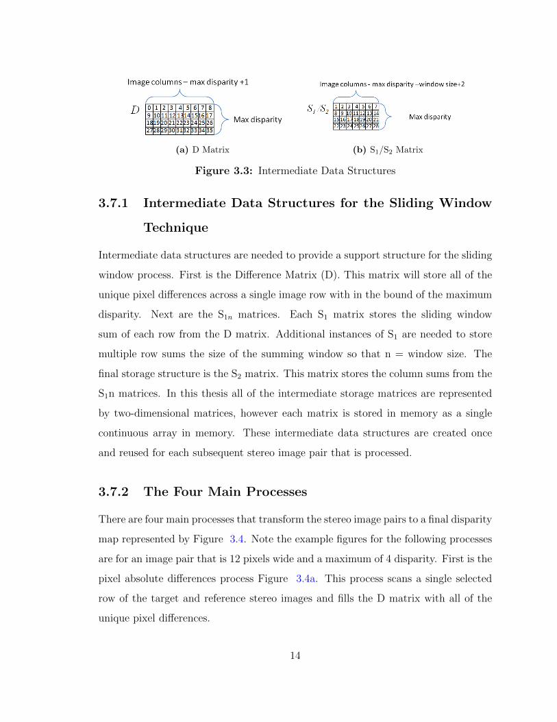
(a) D Matrix (b) S1/S2 Matrix
Figure 3.3: Intermediate Data Structures
3.7.1 Intermediate Data Structures for the Sliding Window
Technique
Intermediate data structures are needed to provide a support structure for the sliding
window process. First is the Difference Matrix (D). This matrix will store all of the
unique pixel differences across a single image row with in the bound of the maximum
disparity. Next are the S1n matrices. Each S1 matrix stores the sliding window
sum of each row from the D matrix. Additional instances of S1 are needed to store
multiple row sums the size of the summing window so that n = window size. The
final storage structure is the S2 matrix. This matrix stores the column sums from the
S1n matrices. In this thesis all of the intermediate storage matrices are represented
by two-dimensional matrices, however each matrix is stored in memory as a single
continuous array in memory. These intermediate data structures are created once
and reused for each subsequent stereo image pair that is processed.
3.7.2 The Four Main Processes
There are four main processes that transform the stereo image pairs to a final disparity
map represented by Figure 3.4. Note the example figures for the following processes
are for an image pair that is 12 pixels wide and a maximum of 4 disparity. First is the
pixel absolute differences process Figure 3.4a. This process scans a single selected
row of the target and reference stereo images and fills the D matrix with all of the
unique pixel differences.
14
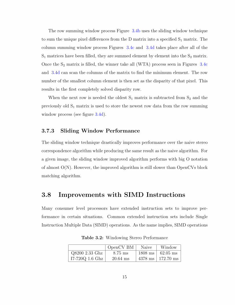
The row summing window process Figure 3.4b uses the sliding window technique
to sum the unique pixel differences from the D matrix into a specified S1 matrix. The
column summing window process Figures 3.4c and 3.4d takes place after all of the
S1 matrices have been filled, they are summed element by element into the S2 matrix.
Once the S2 matrix is filled, the winner take all (WTA) process seen in Figures 3.4c
and 3.4d can scan the columns of the matrix to find the minimum element. The row
number of the smallest column element is then set as the disparity of that pixel. This
results in the first completely solved disparity row.
When the next row is needed the oldest S1 matrix is subtracted from S2 and the
previously old S1 matrix is used to store the newest row data from the row summing
window process (see figure 3.4d).
3.7.3 Sliding Window Performance
The sliding window technique drastically improves performance over the naive stereo
correspondence algorithm while producing the same result as the naive algorithm. For
a given image, the sliding window improved algorithm performs with big O notation
of almost O(N). However, the improved algorithm is still slower than OpenCVs block
matching algorithm.
3.8 Improvements with SIMD Instructions
Many consumer level processors have extended instruction sets to improve per-
formance in certain situations. Common extended instruction sets include Single
Instruction Multiple Data (SIMD) operations. As the name implies, SIMD operations
Table 3.2: Windowing Stereo Performance
OpenCV BM Naive WindowQ8200 2.33 Ghz 8.75 ms 1808 ms 62.05 msI7-720Q 1.6 Ghz 20.64 ms 4378 ms 172.70 ms
15
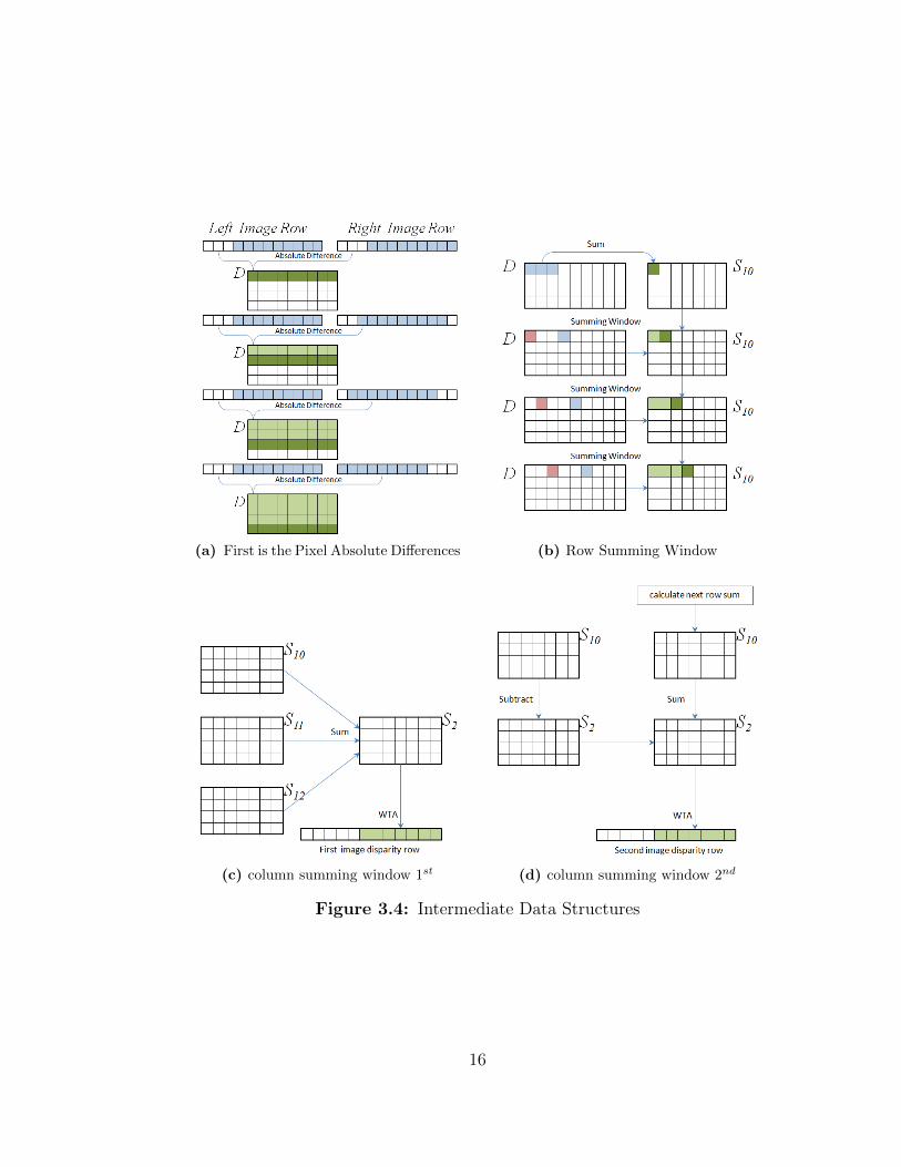
(a) First is the Pixel Absolute Differences (b) Row Summing Window
(c) column summing window 1st (d) column summing window 2nd
Figure 3.4: Intermediate Data Structures
16
are able to process an array of data with the same instruction in a single operation.
For arrays and matrices of data, this can drastically improve computation time
performance.
A number of different processor manufactures have built technologies into their
chips to support SIMD operations. They include ARM with NEON, AMD with
3DNow, and Intel with MMX, Streaming SIMD Extensions (SSE), and Advanced
Vector Extensions (AVE). SSE operations will be using in this thesis since it is the
most widely supported processor extension, supported across multiple Intel and AMD
processors. While SSE will only be only technology used, expanding the code in this
thesis to another SIMD technology is trivial once the code is optimally vectorized.
3.8.1 Intel SSE overview
The Intel SSE introduces a set of 128-bit registers, separate from the standard CPU
registers, that can be packed with a number of different data types. Eight (8)
registers are available for x86 (32-bit processors and operating systems) and sixteen
(16) registers for x64 (64-bit processors and operating systems).
There are several revisions of SSE that have incrementally added new operations.
SSE was first introduced in 1999 and followed by revisions every few years. SSE2
in 2001, SSE3 in 2004, Supplemental Streaming SIMD Extensions (SSSE3) in 2006,
and SSE4 in 2004. The first revision of SSE only supported storing and operating on
four (4) 32-bit floating point or integer values stored in the 128-bit registers. With
SSE2, the ability to store and operate on additional data types was added. The SSE
instruction set includes an almost complete set of instructions. It includes arrhythmic,
logical, compare, shuffle, conversion, load, and store operations.
3.8.2 SSE with C++
Processor specific SSE instructions are normally only accessible via direct assembly
instructions. However Intel provides a header file <emmintrin.h> that makes the
17
assembly instructions available in C and C++ via intrinsic functions. Intrinsics are
basic C mappings for assembly routines that are directly inserted into the main code.
An additional requirement to read memory efficiently into the SSE registers is that
the memory needs to be 16-byte aligned. Where the starting memory address of
the 16-byte segment is a multiple of 16(sixteen). There are instructions to support
loading unaligned memory segments into the SSE registers, but they are considerably
slower. declaring an array of memory requires the use of the aligned malloc function
Microsoft Developer Network (2005). This function will grantee that the starting
point of an array is 16-byte aligned, but will not grantee the entire array will fit in
the 16-byte aligned space. This is the prime reason that OpenCVs block matching
stereo algorithm limits the size of the maximum disparity to multiples of 16.
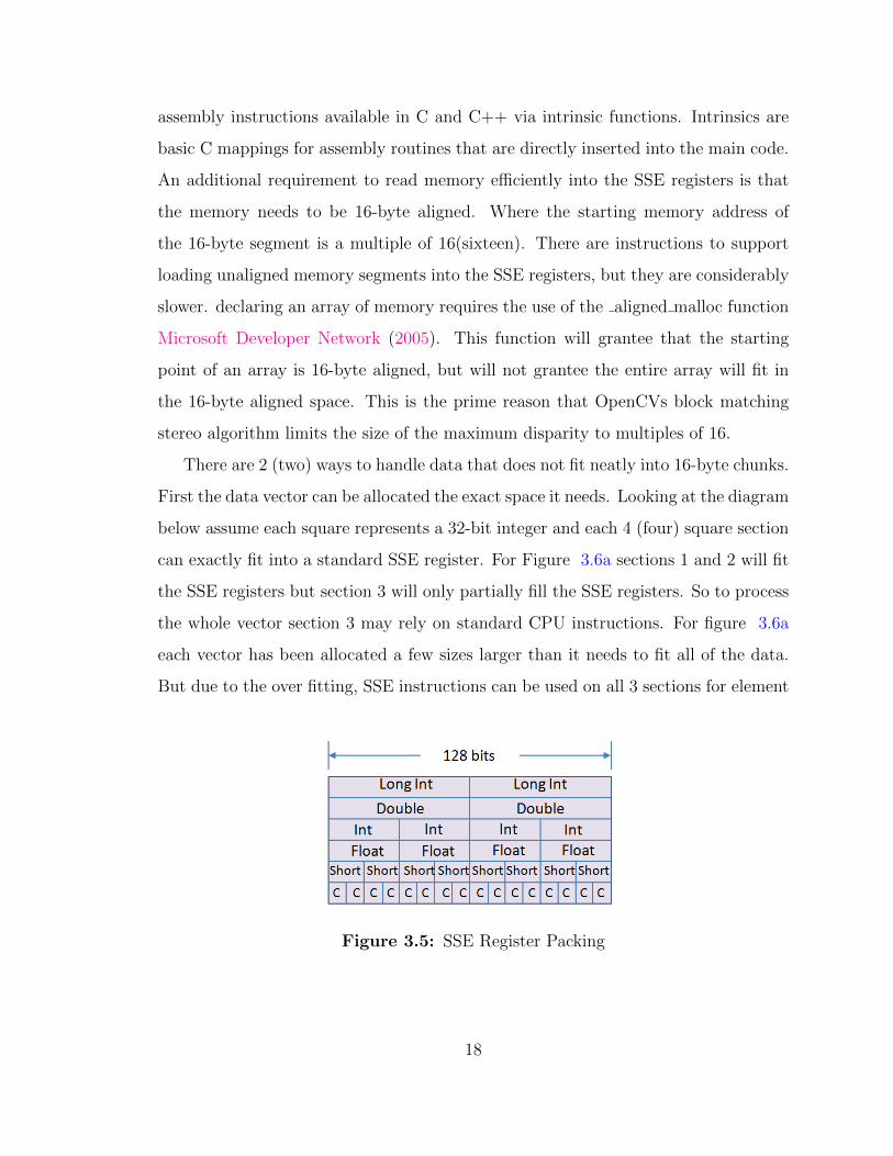
There are 2 (two) ways to handle data that does not fit neatly into 16-byte chunks.
First the data vector can be allocated the exact space it needs. Looking at the diagram
below assume each square represents a 32-bit integer and each 4 (four) square section
can exactly fit into a standard SSE register. For Figure 3.6a sections 1 and 2 will fit
the SSE registers but section 3 will only partially fill the SSE registers. So to process
the whole vector section 3 may rely on standard CPU instructions. For figure 3.6a
each vector has been allocated a few sizes larger than it needs to fit all of the data.
But due to the over fitting, SSE instructions can be used on all 3 sections for element
Figure 3.5: SSE Register Packing
18
by element operations where the extra random data will not pollute the resulting
vector. The over fitting method is used is used in this thesis.
3.8.3 Changes in Intermediate Data Structures for SSE
Applying the over fitting method to the existing intermediate data structures produces
something similar to Figure 3.7. The figure, like before, is for a stereo image pair
with a 12 pixel width and maximum disparity of 4. For each matrix row, filler data is
added at the end so each row will be a multiple of 16 bytes. If the only operations to
be performed on the matrices were element by element, fill data would only needed
to be added on the end of the matrix. But for the winner take all process to work
efficiently the SSE registers need to iterate vertically and horizontally though the
matrix.
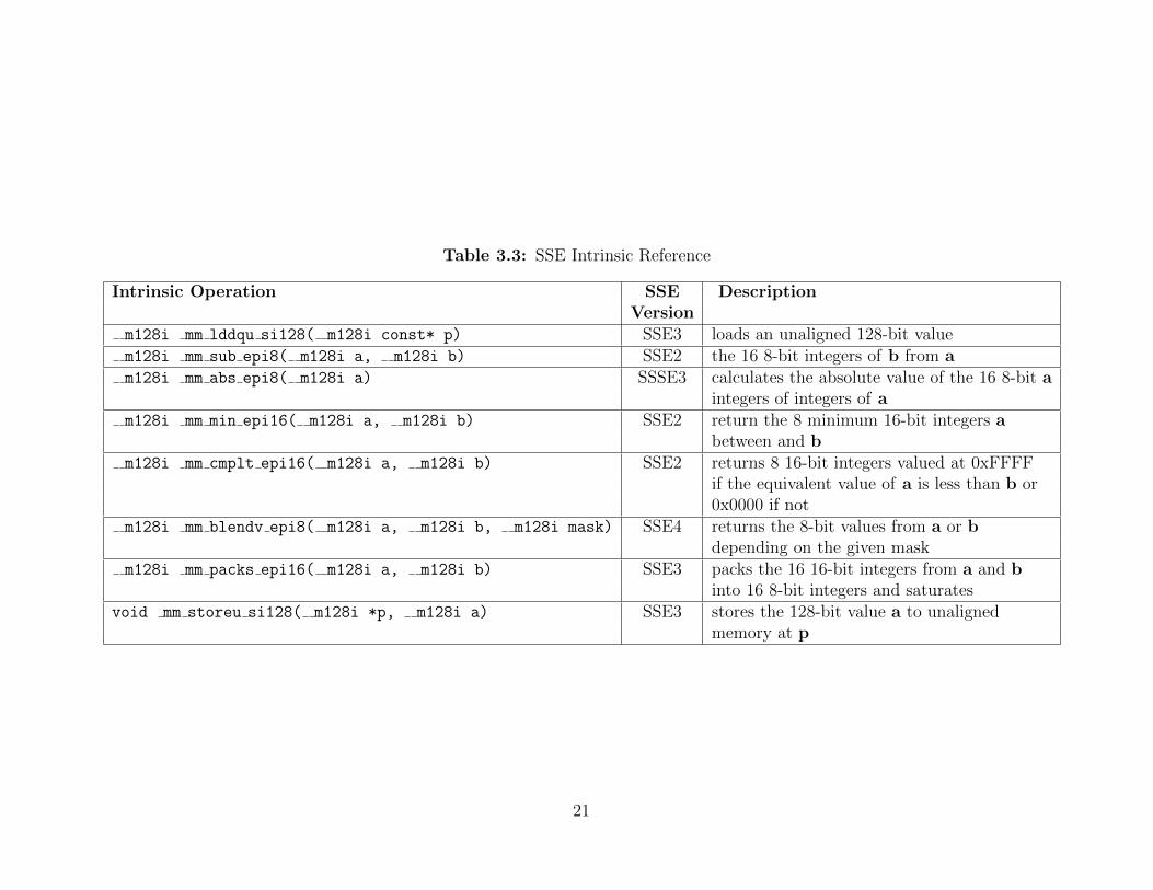
3.8.4 SSE Intrinsics Overview
There are many SSE intrinsics (C++ mapped assembly instructions) but only a few
are needed in this thesis’s algorithm. The Table 3.3 contains a list and description of
all the the SSE intrinsic functions that are used in this thesis. Note the SSE version
number after each description, the highest version number will be the limiting factor
for supported processors. Kowal (2011)
3.8.5 SSE Row Difference
The row difference process like before takes the absolute differences from the left and
right image rows at the zero disparity to the maximum disparity. The SSE intrinsic
functions improve the process by allowing 16 bytes to be processed at the same time
(note that in Figure 3.8 only 4 numbers are being processed in a single SSE instruction
for simplicity). First a 16 byte unaligned chunk from each image row are loaded into
the SSE registers with the mm loadu si128 instruction.
19
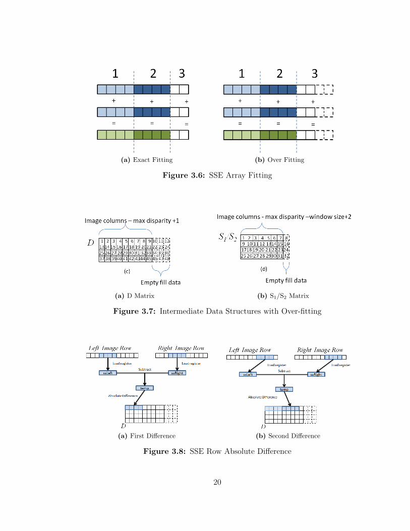
(a) Exact Fitting (b) Over Fitting
Figure 3.6: SSE Array Fitting
(a) D Matrix (b) S1/S2 Matrix
Figure 3.7: Intermediate Data Structures with Over-fitting
(a) First Difference (b) Second Difference
Figure 3.8: SSE Row Absolute Difference
20
21
Table 3.3: SSE Intrinsic Reference
Intrinsic Operation SSE DescriptionVersion
m128i mm lddqu si128( m128i const* p) SSE3 loads an unaligned 128-bit valuem128i mm sub epi8( m128i a, m128i b) SSE2 the 16 8-bit integers of b from am128i mm abs epi8( m128i a) SSSE3 calculates the absolute value of the 16 8-bit a
integers of integers of am128i mm min epi16( m128i a, m128i b) SSE2 return the 8 minimum 16-bit integers a
between and bm128i mm cmplt epi16( m128i a, m128i b) SSE2 returns 8 16-bit integers valued at 0xFFFF
if the equivalent value of a is less than b or0x0000 if not
m128i mm blendv epi8( m128i a, m128i b, m128i mask) SSE4 returns the 8-bit values from a or bdepending on the given mask
m128i mm packs epi16( m128i a, m128i b) SSE3 packs the 16 16-bit integers from a and binto 16 8-bit integers and saturates
void mm storeu si128( m128i *p, m128i a) SSE3 stores the 128-bit value a to unalignedmemory at p
The two registers are subtracted and have their absolute value taken with the
mm sub epi8 and mm abs epi8 instructions. The resulting SSE register is stored
into aligned memory. The inner most while loop iterates this process horizontally
across the matrix while the outer for loop iterates the process vertically over the
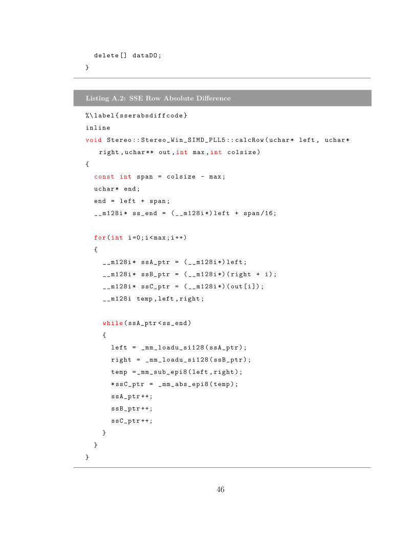
different disparities. See C++ code in Appendix A.2.
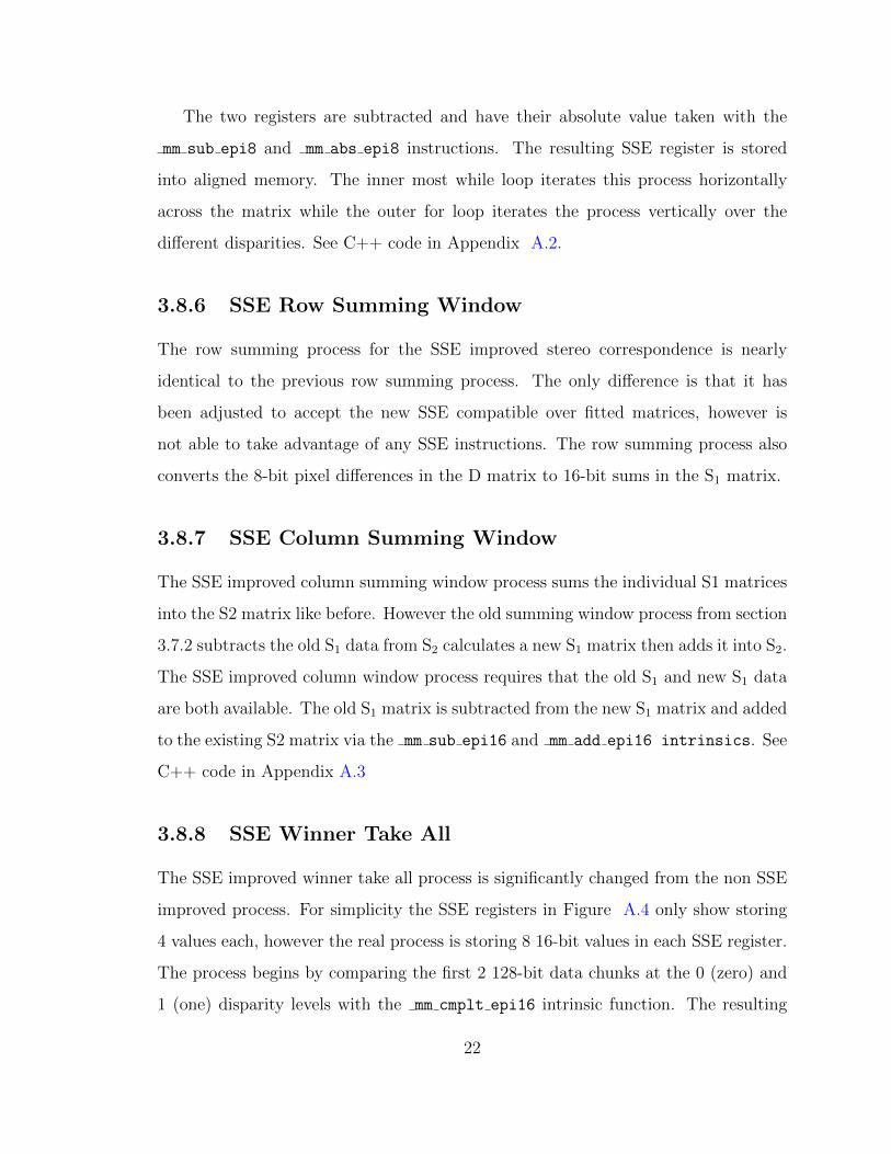
3.8.6 SSE Row Summing Window
The row summing process for the SSE improved stereo correspondence is nearly
identical to the previous row summing process. The only difference is that it has
been adjusted to accept the new SSE compatible over fitted matrices, however is
not able to take advantage of any SSE instructions. The row summing process also
converts the 8-bit pixel differences in the D matrix to 16-bit sums in the S1 matrix.
3.8.7 SSE Column Summing Window
The SSE improved column summing window process sums the individual S1 matrices
into the S2 matrix like before. However the old summing window process from section
3.7.2 subtracts the old S1 data from S2 calculates a new S1 matrix then adds it into S2.
The SSE improved column window process requires that the old S1 and new S1 data
are both available. The old S1 matrix is subtracted from the new S1 matrix and added
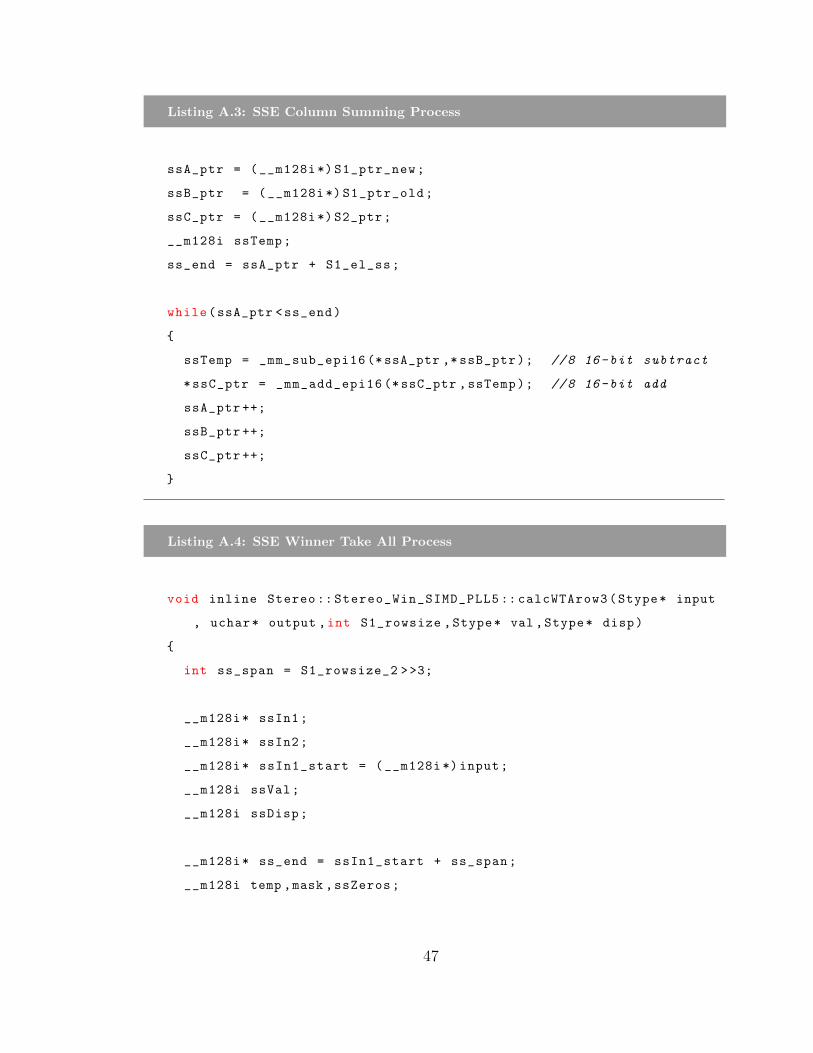
to the existing S2 matrix via the mm sub epi16 and mm add epi16 intrinsics. See
C++ code in Appendix A.3
3.8.8 SSE Winner Take All
The SSE improved winner take all process is significantly changed from the non SSE
improved process. For simplicity the SSE registers in Figure A.4 only show storing
4 values each, however the real process is storing 8 16-bit values in each SSE register.
The process begins by comparing the first 2 128-bit data chunks at the 0 (zero) and
1 (one) disparity levels with the mm cmplt epi16 intrinsic function. The resulting
22
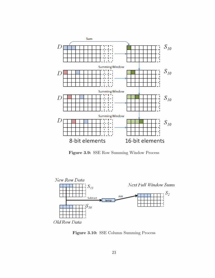
Figure 3.9: SSE Row Summing Window Process
Figure 3.10: SSE Column Summing Process
23
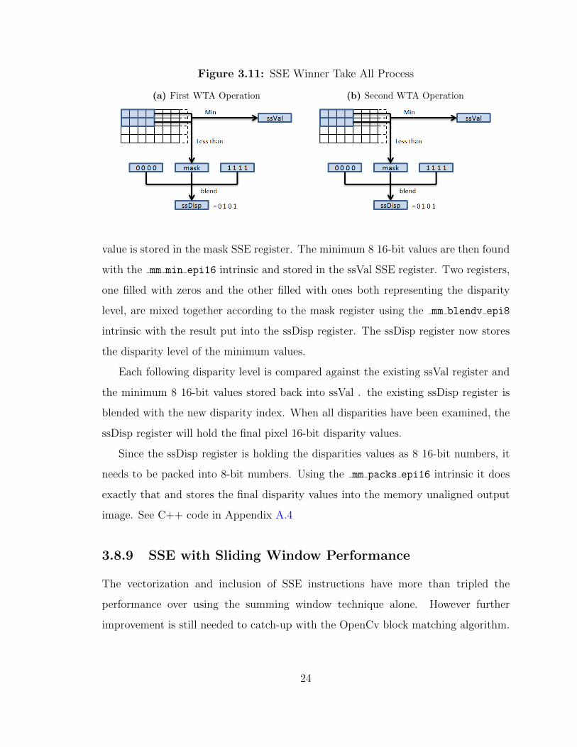
Figure 3.11: SSE Winner Take All Process
(a) First WTA Operation (b) Second WTA Operation
value is stored in the mask SSE register. The minimum 8 16-bit values are then found
with the mm min epi16 intrinsic and stored in the ssVal SSE register. Two registers,
one filled with zeros and the other filled with ones both representing the disparity
level, are mixed together according to the mask register using the mm blendv epi8
intrinsic with the result put into the ssDisp register. The ssDisp register now stores
the disparity level of the minimum values.
Each following disparity level is compared against the existing ssVal register and
the minimum 8 16-bit values stored back into ssVal . the existing ssDisp register is
blended with the new disparity index. When all disparities have been examined, the
ssDisp register will hold the final pixel 16-bit disparity values.
Since the ssDisp register is holding the disparities values as 8 16-bit numbers, it
needs to be packed into 8-bit numbers. Using the mm packs epi16 intrinsic it does
exactly that and stores the final disparity values into the memory unaligned output
image. See C++ code in Appendix A.4
3.8.9 SSE with Sliding Window Performance
The vectorization and inclusion of SSE instructions have more than tripled the
performance over using the summing window technique alone. However further
improvement is still needed to catch-up with the OpenCv block matching algorithm.
24
3.9 Improving performance with Parallelism
While consumer level CPUs are available at greater speeds every year, the physical
limit of processor speed is quickly approaching. To keep improving performance with
each new generation, processor manufactures have been adding multi-core support
to their processors. However implementing multi-threaded support to the algorithm
adds new problems.
First developing multi-threaded processes is not natively supported by C++ and
requires operating system specific functions to start new threads. For any cross
platform project, this is a huge hindrance. There are several packages available the
bridges the platform gap in multi-threading such as the Boost libraries, the Intel
Threading Building Blocks (TBB), and the updated C++11 standard that includes a
thread object in the standard template library. This thesis uses the Intel Threading
Building Blocks.
Other problems introduced with parallelism are shared resources, race conditions,
and deadlocks. While there are a number of techniques to manage and avoid these
problems, this thesis avoids most of them by having completely separate instances
of intermediate data for each thread and does not allow threads to pass data to one
another. This technique is sometimes call embarrassingly parallel.
3.9.1 Dividing the Data
To easily manage the threaded data, the stereo image pair is separated into separate
independent stereo matching problems. In the example at Figure 3.12, the stereo
image pair is separated into two stereo matching problems that can be solved in
parallel then stitched back together for the whole depth mapped image. For the
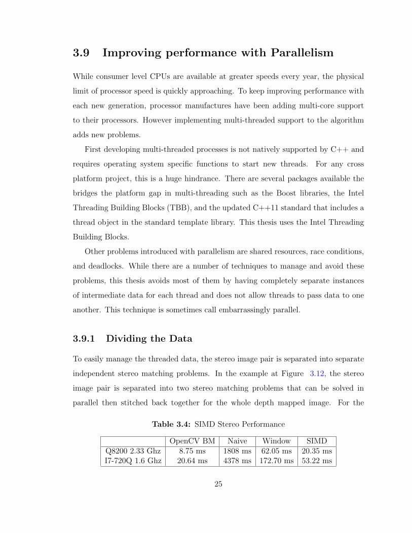
Table 3.4: SIMD Stereo Performance
OpenCV BM Naive Window SIMDQ8200 2.33 Ghz 8.75 ms 1808 ms 62.05 ms 20.35 msI7-720Q 1.6 Ghz 20.64 ms 4378 ms 172.70 ms 53.22 ms
25
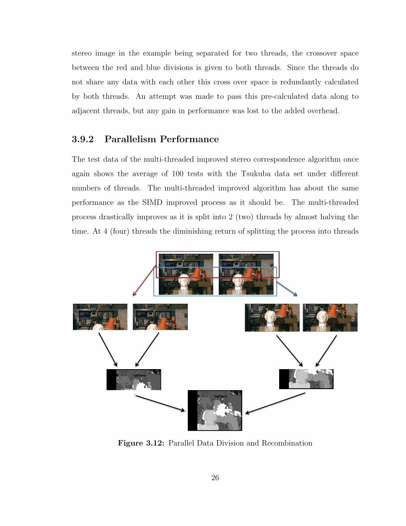
stereo image in the example being separated for two threads, the crossover space
between the red and blue divisions is given to both threads. Since the threads do
not share any data with each other this cross over space is redundantly calculated
by both threads. An attempt was made to pass this pre-calculated data along to
adjacent threads, but any gain in performance was lost to the added overhead.
3.9.2 Parallelism Performance
The test data of the multi-threaded improved stereo correspondence algorithm once
again shows the average of 100 tests with the Tsukuba data set under different
numbers of threads. The multi-threaded improved algorithm has about the same
performance as the SIMD improved process as it should be. The multi-threaded
process drastically improves as it is split into 2 (two) threads by almost halving the
time. At 4 (four) threads the diminishing return of splitting the process into threads
Figure 3.12: Parallel Data Division and Recombination
26
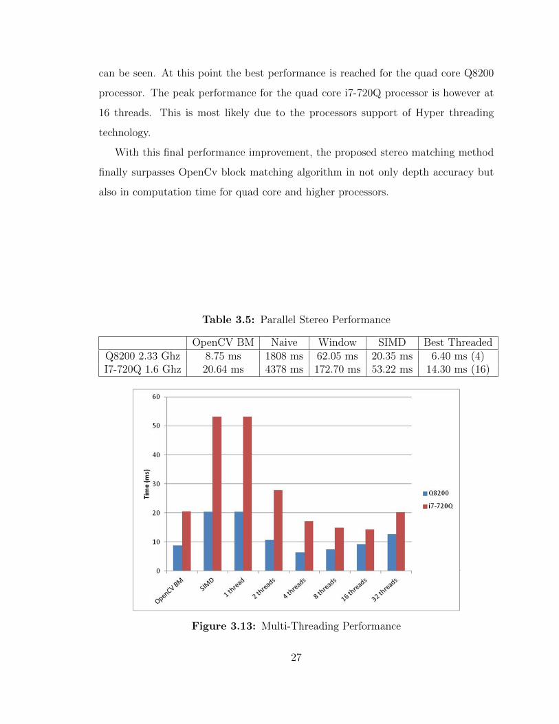
can be seen. At this point the best performance is reached for the quad core Q8200
processor. The peak performance for the quad core i7-720Q processor is however at
16 threads. This is most likely due to the processors support of Hyper threading
technology.
With this final performance improvement, the proposed stereo matching method
finally surpasses OpenCv block matching algorithm in not only depth accuracy but
also in computation time for quad core and higher processors.
Table 3.5: Parallel Stereo Performance
OpenCV BM Naive Window SIMD Best ThreadedQ8200 2.33 Ghz 8.75 ms 1808 ms 62.05 ms 20.35 ms 6.40 ms (4)I7-720Q 1.6 Ghz 20.64 ms 4378 ms 172.70 ms 53.22 ms 14.30 ms (16)
Figure 3.13: Multi-Threading Performance
27
Chapter 4
Applying Stereo Method to Real
Cameras
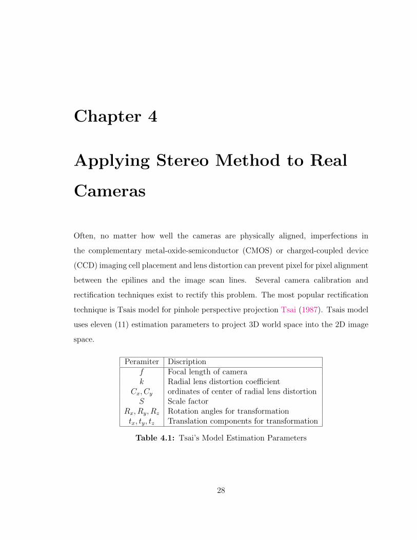
Often, no matter how well the cameras are physically aligned, imperfections in
the complementary metal-oxide-semiconductor (CMOS) or charged-coupled device
(CCD) imaging cell placement and lens distortion can prevent pixel for pixel alignment
between the epilines and the image scan lines. Several camera calibration and
rectification techniques exist to rectify this problem. The most popular rectification
technique is Tsais model for pinhole perspective projection Tsai (1987). Tsais model
uses eleven (11) estimation parameters to project 3D world space into the 2D image
space.
Peramiter Discriptionf Focal length of camerak Radial lens distortion coefficient
Cx, Cy ordinates of center of radial lens distortionS Scale factor
Rx, Ry, Rz Rotation angles for transformationtx, ty, tz Translation components for transformation
Table 4.1: Tsai’s Model Estimation Parameters
28
4.1 Calibration
To properly set the estimation parameters in Tsai’s camera model, a set of calibration
images with a known calibration pattern such as a checker board can be used. knowing
the exact size of the checker board, the exact location in 3D space of the checker
board can be found only with the 2D image. With several images of checker boards
at different angles and depths from the camera, a gradient decent function may solve
for the best estimation parameters for the pin hole camera model.
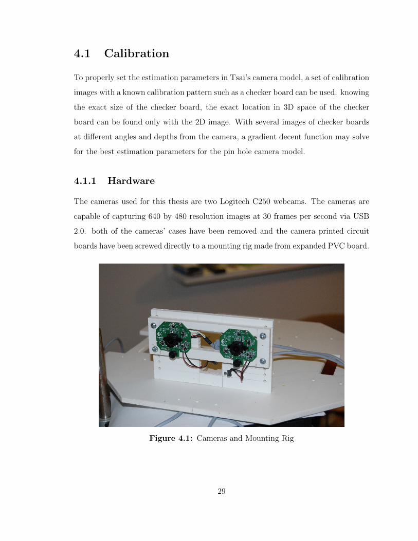
4.1.1 Hardware
The cameras used for this thesis are two Logitech C250 webcams. The cameras are
capable of capturing 640 by 480 resolution images at 30 frames per second via USB
2.0. both of the cameras’ cases have been removed and the camera printed circuit
boards have been screwed directly to a mounting rig made from expanded PVC board.
Figure 4.1: Cameras and Mounting Rig
29
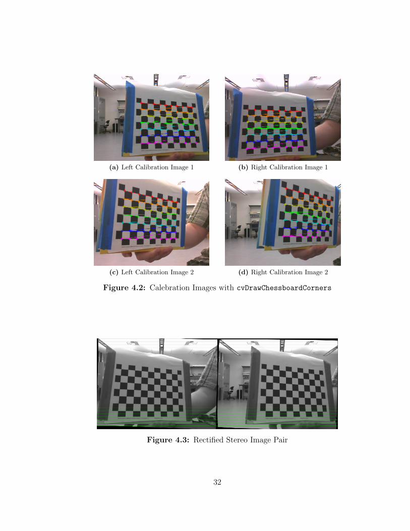
4.1.2 Calibration Procedure
To begin calibrating, a chessboard patterned calibration target is chosen. The
chessboard pattern may have any number of rows and columns; however having
less than five (5) in either dimension may reduce the quality of the rectified
result. The chessboard maybe printed on paper but it needs a firm backing. Any
physical distortion of the chessboard pattern will significantly reduce the accuracy of
calibration. Note that choosing black and white for chessboard test image gives the
maximum contrast for the next set of algorithms to detect the checkerboard corners.
The chessboard test pattern below is printed on an 8 x11.5 piece of paper and taped
to the face of a book. The test pattern has 2.0 cm wide squares with 11 columns and
8 rows.
Acquiring a set of test images is fairly simple. First the test pattern is presented
in front of the stereo cameras. The pattern needs to be in full view of both cameras.
A snap shot is taken and saved to memory or a file. Though experimentation, five (5)
image pairs seems to be sufficient to calibrate the stereo cameras. Using too many
calibration image pairs may make OpenCVs calibration using Hartleys algorithm
Hartley (1992) may take an excessive amount of time to reach its final values, or
worse my never converge to a final set of camera calibration constants.
To extract the chessboard point data, OpenCV provides the function
cvFindChessboardCorners. The function only needs to know the number of
chessboard cross sections vertically and horizontally and will return an array
of point where the cross sections are at. OpenCV provides another function
cvFindCornerSubPix to better refine the found chessboard corners to sub-pixel
accuracy. The results of the detected chessboard corners can be displayed on the
image via cvDrawChessboardCorners.
Once all of the chessboard corners have been harvested from the image pairs, the
point can be feed into another OpenCV function cvStereoCalibrate. This function
is based on Hartleys stereo camera calibration algorithm. The algorithm will compute
30
the best fitted estimation values for Tsais pinhole camera model ?Tsai) so that the
epipolar lines will be row aligned with each other.
4.2 Real-time Rectification
While it would be simple to apply Tsais transforms directly to the stereo image
pair for every video frame, it would take too much processing time for the real-time
requirements. Instead, the camera model is used to calculate a large lookup table that
represents the remapping of each individual pixel in an image. This method speeds
up the image correction time at the expense of system memory. OpenCV once again
provides the function remap that will remap and image given a mapping table. The
OpenCV remap function requires two (2) tables one for the horizontal mapping and
the other for vertical mapping. Both tables store the remapped sub-pixel locations
as 32-bit floating point numbers. This allows the function to use a number of pixel
interpolation methods such as nearest-neighbor, bilinear, bicubic, and lanczos. For
the purposes of this thesis, the least accurate but fastest of the methods, nearest-
neighbor, is used to remap the Images. But because the OpenCV remap function is
designed to support these multiple interpolation methods, it is not well optimized for
nearest- neighbor specifically. To get the best performance out of remapping, a new
function is programmed that is optimized in three (3) specific ways.
4.2.1 Optimized Nearest-Neighbor
First the mapping tables are pre-calculated to their nearest-neighbor pixel and stored
into a single table. The table no longer points to the horizontal and vertical pixel
locations in the image, but now point to the memory offset locations in the image pixel
array stored in memory. The second optimization only works for full color images.
In the original OpenCV remap function, each color channel (Red, Green, and Blue)
is copied separately 1 byte at a time. In the new remap function the red, green, and
31
(a) Left Calibration Image 1 (b) Right Calibration Image 1
(c) Left Calibration Image 2 (d) Right Calibration Image 2
Figure 4.2: Calebration Images with cvDrawChessboardCorners
Figure 4.3: Rectified Stereo Image Pair
32
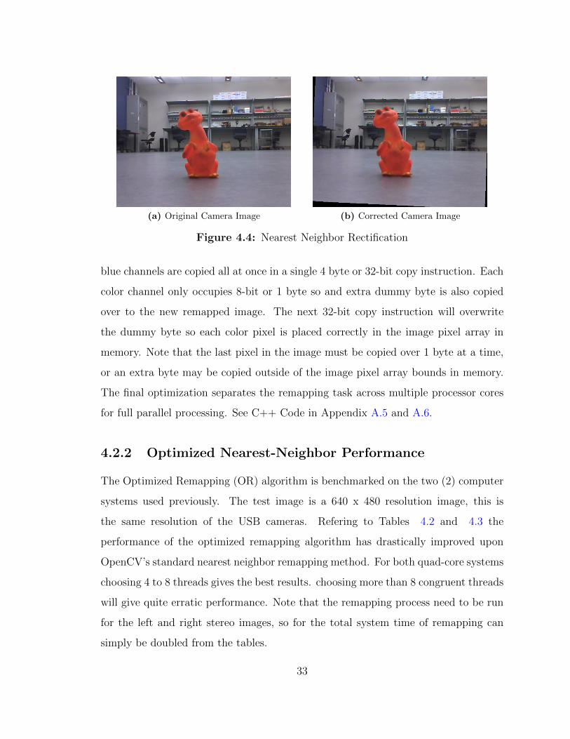
(a) Original Camera Image (b) Corrected Camera Image
Figure 4.4: Nearest Neighbor Rectification
blue channels are copied all at once in a single 4 byte or 32-bit copy instruction. Each
color channel only occupies 8-bit or 1 byte so and extra dummy byte is also copied
over to the new remapped image. The next 32-bit copy instruction will overwrite
the dummy byte so each color pixel is placed correctly in the image pixel array in
memory. Note that the last pixel in the image must be copied over 1 byte at a time,
or an extra byte may be copied outside of the image pixel array bounds in memory.
The final optimization separates the remapping task across multiple processor cores
for full parallel processing. See C++ Code in Appendix A.5 and A.6.
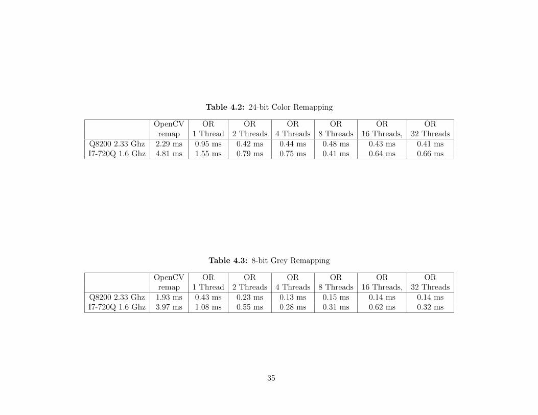
4.2.2 Optimized Nearest-Neighbor Performance
The Optimized Remapping (OR) algorithm is benchmarked on the two (2) computer
systems used previously. The test image is a 640 x 480 resolution image, this is
the same resolution of the USB cameras. Refering to Tables 4.2 and 4.3 the
performance of the optimized remapping algorithm has drastically improved upon
OpenCV’s standard nearest neighbor remapping method. For both quad-core systems
choosing 4 to 8 threads gives the best results. choosing more than 8 congruent threads
will give quite erratic performance. Note that the remapping process need to be run
for the left and right stereo images, so for the total system time of remapping can
simply be doubled from the tables.
33
4.3 Complete System
The complete stereo correspondence system begins with capturing images from the
cameras with OpenCV’s VideoCapture module. The VideoCapture module will
retrieve the two images from the camera in an easy to manipulate cv::Mat object. If
the VideoCapture module is called faster then the camera’s frame rate will allow, the
module will simply block execution until the camera is ready. the Logitech USB web
cameras used in this thesis are limited to 30 frames per second. the stereo images
are then passed to OpenCV’s cv::cvtColor function and converts the 24-bit color
images to 8-bit grey scale. This color conversion is necessary since Both OpenCV’s
block matching and this thesis proposed methods can only parse 8-bit images.
Once the stereo images are gray, they are rectified with this thesis’s optimized
rectification algorithm from section 4.2.1. The rectified stereo images are now passed
to this thesis’s proposed stereo block matching method and produce the final disparity
image. since this thesis is only developing the block matching method, the disparity
map is displayed to the screen and returns to the main loop to acquire another stereo
image pair from the cameras. However, for an autonomous robot, further processing
of the disparity map is required to effectively use it. Mainly the disparity map would
be used for object detection and/or avoidance.
34
35
Table 4.2: 24-bit Color Remapping
OpenCV OR OR OR OR OR ORremap 1 Thread 2 Threads 4 Threads 8 Threads 16 Threads, 32 Threads
Q8200 2.33 Ghz 2.29 ms 0.95 ms 0.42 ms 0.44 ms 0.48 ms 0.43 ms 0.41 msI7-720Q 1.6 Ghz 4.81 ms 1.55 ms 0.79 ms 0.75 ms 0.41 ms 0.64 ms 0.66 ms
Table 4.3: 8-bit Grey Remapping
OpenCV OR OR OR OR OR ORremap 1 Thread 2 Threads 4 Threads 8 Threads 16 Threads, 32 Threads
Q8200 2.33 Ghz 1.93 ms 0.43 ms 0.23 ms 0.13 ms 0.15 ms 0.14 ms 0.14 msI7-720Q 1.6 Ghz 3.97 ms 1.08 ms 0.55 ms 0.28 ms 0.31 ms 0.62 ms 0.32 ms
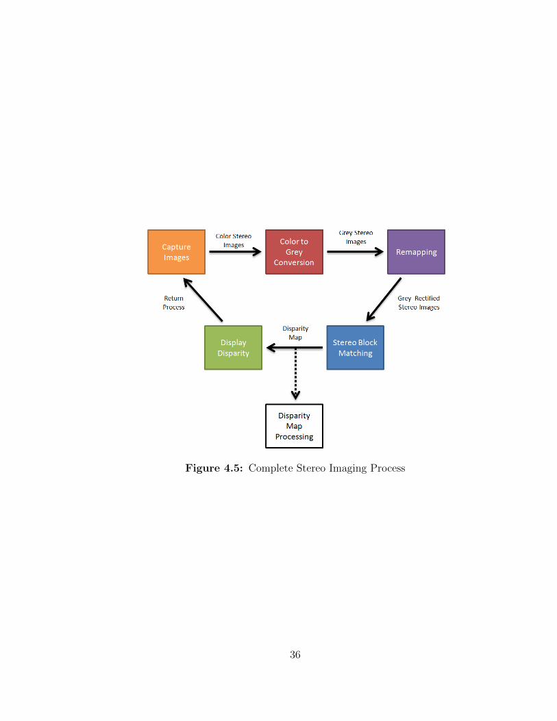
Figure 4.5: Complete Stereo Imaging Process
36
Chapter 5
Conclusions and Future Work
5.1 Conclusions
This thesis’s proposed stereo block matching method is able to surpass OpenCV’s
block matching method in quality and processing time in quad core systems. For
single and dual core systems OpenCV’s method is superior in processing time.
Additionally this paper’s method of block matching is not limited to window sizes
at multiples of sixteen (16) as in the OpenCV’s block matching method, thanks the
use of over-fitting the intermediate data structures for the SIMD operations.
5.2 Future Work
Continued work on this thesis’s method will include expanding the supported
architecture the stereo block matching method uses. First, Intel’s Advances Vector
Extensions (AVE), a 256-bit extension of the SSE instruction set, will be added for
greater performance in Intel Sandy and Ivy Bridge processors. Next, ARM’s SIMD
instruction set, NEON, may be added for their chip-sets.
Since OpenCV’s block matching method still runs quicker for single core systems,
there may still be room for improvement in optimizing the code. Further improvement
37

may come from directly optimizing critical loop sections in assembly language to
efficiently stream image data.
The disparity image quality may also be improved by implementing uniqueness
testing in the winner take all method or by applying pre-filters to the stereo image
pair.
38

Bibliography
39
Bibliography
Hartley, R. I. (1992). Estimation of relative camera positions for uncalibrated
cameras. In Proceedings of the Second European Conference on Computer Vision,
pages 579–587. Springer-Verlag. 30
Hirschmuller, H. Scharstein, D. (2007). Evaluation of cost functions for stereo
matching. In Computer Vision and Pattern Recognition, 2007. CVPR ’07. IEEE
Conference on, pages 1–8. 5, 7
Kowal, G. (2011). Intrinsics guide for intel advanced vector extensions 2. 19
Kuk-Jin, Yoon In So, K. (2006). Adaptive support-weight approach for
correspondence search. Pattern Analysis and Machine Intelligence, IEEE
Transactions on, 28:650–656. 6
Microsoft Developer Network (2005). aligned malloc. 18
Muhlmann, K. Maier, D. H. R. M. R. (2001). Calculating dense disparity maps
from color stereo images, an efficient implementation. In Stereo and Multi-Baseline
Vision, 2001. (SMBV 2001). Proceedings. IEEE Workshop on. 13
Scharstein, D. Szeliski, R. Z. R. (2001). A taxonomy and evaluation of dense two-
frame stereo correspondence algorithms. In Stereo and Multi-Baseline Vision, 2001.
(SMBV 2001). Proceedings. IEEE Workshop on, pages 131–140. 5, 6, 12
40

Tsai, R. (1987). A versatile camera calibration technique for high-accuracy 3d
machine vision metrology using off-the-shelf tv cameras and lenses. Robotics and
Automation, IEEE Journal of, 3:323–344. 28
41

Appendix
42
Appendix A
Listings of Code
A.1 Chapter 3 Code
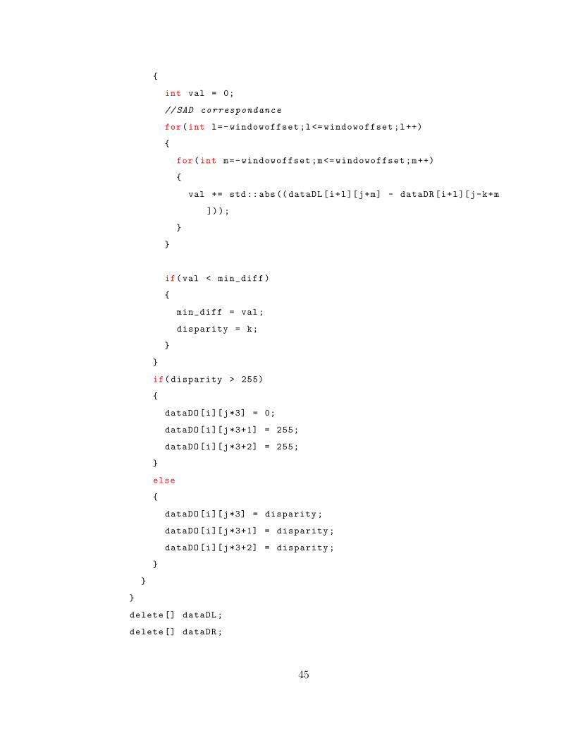
Listing A.1: Naive Stereo Matching
void Stereo ::SAD:: stVisual(cv::Mat &leftImg , cv::Mat &rightImg , cv
::Mat &outImg)
{
// both stereo images must match
CV_Assert(leftImg.size() == rightImg.size());
CV_Assert(leftImg.type() == rightImg.type());
cv::Mat displayL;
cv::Mat displayR;
cv::Mat displayO;
if(leftImg.size() != outImg.size() || outImg.type() != CV_8UC1)
{
outImg.release ();
outImg.create(leftImg.size(),CV_8UC3);
for(int i=0;i<leftImg.rows*leftImg.cols *3;i++)
outImg.data[i] = 0;
}
43
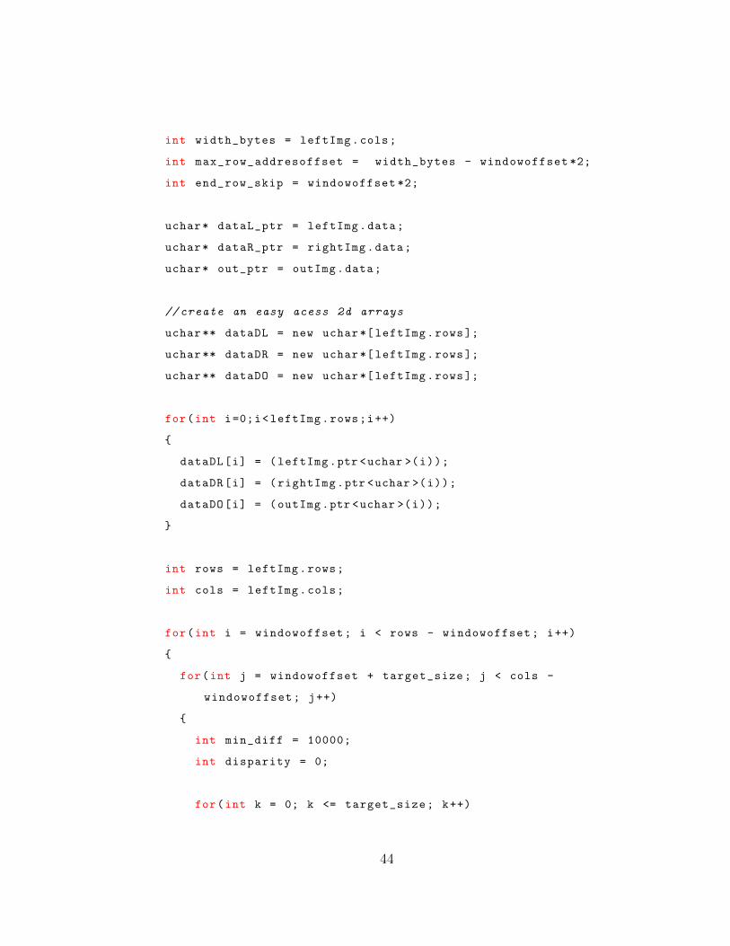
int width_bytes = leftImg.cols;
int max_row_addresoffset = width_bytes - windowoffset *2;
int end_row_skip = windowoffset *2;
uchar* dataL_ptr = leftImg.data;
uchar* dataR_ptr = rightImg.data;
uchar* out_ptr = outImg.data;
// create an easy acess 2d arrays
uchar ** dataDL = new uchar *[ leftImg.rows];
uchar ** dataDR = new uchar *[ leftImg.rows];
uchar ** dataDO = new uchar *[ leftImg.rows];
for(int i=0;i<leftImg.rows;i++)
{
dataDL[i] = (leftImg.ptr <uchar >(i));
dataDR[i] = (rightImg.ptr <uchar >(i));
dataDO[i] = (outImg.ptr <uchar >(i));
}
int rows = leftImg.rows;
int cols = leftImg.cols;
for(int i = windowoffset; i < rows - windowoffset; i++)
{
for(int j = windowoffset + target_size; j < cols -
windowoffset; j++)
{
int min_diff = 10000;
int disparity = 0;
for(int k = 0; k <= target_size; k++)
44
{
int val = 0;
//SAD correspondance
for(int l=-windowoffset;l<= windowoffset;l++)
{
for(int m=-windowoffset;m<= windowoffset;m++)
{
val += std::abs(( dataDL[i+l][j+m] - dataDR[i+l][j-k+m
]));
}
}
if(val < min_diff)
{
min_diff = val;
disparity = k;
}
}
if(disparity > 255)
{
dataDO[i][j*3] = 0;
dataDO[i][j*3+1] = 255;
dataDO[i][j*3+2] = 255;
}
else
{
dataDO[i][j*3] = disparity;
dataDO[i][j*3+1] = disparity;
dataDO[i][j*3+2] = disparity;
}
}
}
delete [] dataDL;
delete [] dataDR;
45
delete [] dataDO;
}
Listing A.2: SSE Row Absolute Difference
%\label{sserabsdiffcode}
inline
void Stereo :: Stereo_Win_SIMD_PLL5 :: calcRow(uchar* left , uchar*
right ,uchar** out ,int max ,int colsize)
{
const int span = colsize - max;
uchar* end;
end = left + span;
__m128i* ss_end = (__m128i *)left + span /16;
for(int i=0;i<max;i++)
{
__m128i* ssA_ptr = (__m128i *)left;
__m128i* ssB_ptr = (__m128i *)(right + i);
__m128i* ssC_ptr = (__m128i *)(out[i]);
__m128i temp ,left ,right;
while(ssA_ptr <ss_end)
{
left = _mm_loadu_si128(ssA_ptr);
right = _mm_loadu_si128(ssB_ptr);
temp =_mm_sub_epi8(left ,right);
*ssC_ptr = _mm_abs_epi8(temp);
ssA_ptr ++;
ssB_ptr ++;
ssC_ptr ++;
}
}
}
46
Listing A.3: SSE Column Summing Process
ssA_ptr = (__m128i *) S1_ptr_new;
ssB_ptr = (__m128i *) S1_ptr_old;
ssC_ptr = (__m128i *) S2_ptr;
__m128i ssTemp;
ss_end = ssA_ptr + S1_el_ss;
while(ssA_ptr <ss_end)
{
ssTemp = _mm_sub_epi16 (*ssA_ptr ,* ssB_ptr); //8 16-bit subtract
*ssC_ptr = _mm_add_epi16 (*ssC_ptr ,ssTemp); //8 16-bit add
ssA_ptr ++;
ssB_ptr ++;
ssC_ptr ++;
}
Listing A.4: SSE Winner Take All Process
void inline Stereo :: Stereo_Win_SIMD_PLL5 :: calcWTArow3(Stype* input
, uchar* output ,int S1_rowsize ,Stype* val ,Stype* disp)
{
int ss_span = S1_rowsize_2 >>3;
__m128i* ssIn1;
__m128i* ssIn2;
__m128i* ssIn1_start = (__m128i *) input;
__m128i ssVal;
__m128i ssDisp;
__m128i* ss_end = ssIn1_start + ss_span;
__m128i temp ,mask ,ssZeros;
47
__m128i* ssOut = (__m128i *) output;
int depth_index;
ssZeros = _mm_set1_epi16 (0);
while(ssIn1_start <ss_end)
{
ssIn1 = ssIn1_start;
ssIn2 = ssIn1_start + ss_span;
ssVal = _mm_min_epi16 (*ssIn1 , *ssIn2);
mask = _mm_cmplt_epi16 (*ssIn1 , *ssIn2);
ssDisp = _mm_blendv_epi8(ssZeros ,_mm_set1_epi16 (1),mask);
ssIn2 += ss_span;
depth_index = 2;
while(depth_index <max_disparity)
{
mask = _mm_cmplt_epi16 (*ssIn2 , ssVal);
ssVal = _mm_min_epi16(ssVal , *ssIn2);
ssDisp = _mm_blendv_epi8(ssDisp ,_mm_set1_epi16(depth_index),
mask);
ssIn2 += ss_span;
depth_index ++;
}
temp = _mm_packs_epi16(ssDisp , ssZeros);
_mm_storeu_si128(ssOut , temp);
ssIn1_start ++;
output +=8;
ssOut = (__m128i *) output;
48
}
}
A.2 Chapter 4 Code
Listing A.5: Optimized Grey Scale Nearest-Neighbor Remapping
void refinedCV :: pplremap_grey(const cv::Mat &input , cv::Mat &
output , std::vector <int > &map , int chunksize)
{
// consistancy check
CV_Assert(input.isContinuous ());
CV_Assert ((input.cols*input.rows) == map.size());
// allocate output Mat memmory
if(input.size() != output.size())
{
output.release ();
output.create(input.size(),input.type());
}
//
int chunk_width = map.size()/chunksize;
int map_width = map.size()/chunksize;
int max_addr_offset = map_width;
Concurrency :: parallel_for (0,chunksize ,[&]( int chunk)
{
int m;
int* mapptr = &(map [0]) + map_width*chunk;
uchar* data = output.data + chunk_width*chunk;
uchar* indata ,* input_data;
input_data = input.data;
49
int* maxaddess = mapptr + max_addr_offset;
for(;mapptr <maxaddess;mapptr ++)
{
m = mapptr [0];
if (m < 0)
{
data [0] = 0;
}
else
{
data [0] = input_data[m];
}
data ++;
}
});
}
Listing A.6: Optimized Color Nearest-Neighbor Remapping
void refinedCV :: pplremap_color(const cv::Mat &input , cv::Mat &
output , std::vector <int > &map , int chunksize)
{
// consistancy check
CV_Assert(input.isContinuous ());
CV_Assert ((input.cols*input.rows) == map.size());
// allocate output Mat memmory
if(input.size() != output.size())
{
output.release ();
output.create(input.size(),input.type());
}
50
//
int chunk_width = map.size()*3/ chunksize;
int map_width = map.size()/chunksize;
int max_addr_offset = map_width -1;
Concurrency :: parallel_for (0,chunksize ,[&]( int chunk)
{
int m;
int* mapptr = &(map [0]) + map_width*chunk;
uchar* data = output.data + chunk_width*chunk;
int* indata;
int* maxaddess = mapptr + max_addr_offset;
for(;mapptr <maxaddess;mapptr ++)
{
m = mapptr [0];
if (m < 0)
{
*(int*)data = 0;
}
else
{
indata = (int*)&( input.data[m]);
*(int*)data = *indata;
}
data += 3;
}
m = *mapptr;
if (m == -1)
{
data [0] = 0;
data [1] = 0;
data [2] = 0;
51
}
else
{
indata = (int*)&( input.data[m]);
data [0] = (( uchar*) indata)[0];
data [1] = (( uchar*) indata)[1];
data [2] = (( uchar*) indata)[2];
}
});
}
52
Vita
Bryan Bodkin was born in Los Angeles California, in 1985. After graduating in 2004
from Brentwood High School, He attended Middle Tennessee State University, where
he received a Bachelor of Science in 2009 double majoring in Computer Science and
Electrical Mechanical Engineering Technology. In the Fall of 2009 Bryan enrolled into
the Masters program at the University of Tennessee Knoxville in the department of
Electrical Engineering and Computer Science. A year later he joined the Advanced
Imaging and Collaborative Information Processing (AICIP) group as a research
assistant where he will complete his Master degree in the summer of 2012. His major
research areas are real-time image processing, firmware programming, Graphics User
Interface (GUI) programming, and electric hardware development.
53