MITSUBISHI ELECTRIC RESEARCH LABORATORIEShttp://www.merl.com

Real-time optimization and model predictive control foraerospace and automotive applications

Di Cairano, S.; Kolmanovsky, I.V.

TR2018-086 July 13, 2018

AbstractIn recent years control methods based on realtime optimization (RTO) such as model pre-dictive control (MPC) have been investigated for a significant number of applications in theautomotive and aerospace (A&A) domains. This paper provides a tutorial overview of RTOin automotive and aerospace, with particular focus on MPC which is probably the mostlargely investigated method. First, we review the features that make RTO appealing forA&A applications. Then, due to the model-based nature of these control methods, we de-scribe the key first principle models and opportunities that these provide for RTO. Next, wedetail the key steps and guidelines of the MPC design process which are tailored to A&A sys-tems. Finally, we discuss numerical algorithms for implementing RTO, and their suitabilityfor implementation in embedded computing platforms to in A&A domains

American Control Conference (ACC)

This work may not be copied or reproduced in whole or in part for any commercial purpose. Permission to copy inwhole or in part without payment of fee is granted for nonprofit educational and research purposes provided that allsuch whole or partial copies include the following: a notice that such copying is by permission of Mitsubishi ElectricResearch Laboratories, Inc.; an acknowledgment of the authors and individual contributions to the work; and allapplicable portions of the copyright notice. Copying, reproduction, or republishing for any other purpose shall requirea license with payment of fee to Mitsubishi Electric Research Laboratories, Inc. All rights reserved.

Copyright c© Mitsubishi Electric Research Laboratories, Inc., 2018201 Broadway, Cambridge, Massachusetts 02139

Real-time optimization and model predictive control

for aerospace and automotive applications

Stefano Di Cairano1 Ilya V. Kolmanovsky2

Abstract— In recent years control methods based on real-time optimization (RTO) such as model predictive control(MPC) have been investigated for a significant number ofapplications in the automotive and aerospace (A&A) domains.This paper provides a tutorial overview of RTO in automotiveand aerospace, with particular focus on MPC which is probablythe most largely investigated method. First, we review thefeatures that make RTO appealing for A&A applications. Then,due to the model-based nature of these control methods, wedescribe the key first principle models and opportunities thatthese provide for RTO. Next, we detail the key steps andguidelines of the MPC design process which are tailored toA&A systems. Finally, we discuss numerical algorithms forimplementing RTO, and their suitability for implementationin embedded computing platforms to in A&A domains.

I. INTRODUCTION

There are very few devices as pervasive in our world as

cars. Reports show that close to 90 million cars and light

commercial vehicles were sold in 2016. Recent innovations

in car mechanics, electronics and software have been fast

paced to respond to growing stringency of fuel economy,

emissions and safety regulations, as well as to market-driven

pressures to provide customers with improved performance,

drivability and novel features. While different from automo-

tive system in the amount of distribution and accessibility to

the general public, aerospace systems are also increasingly

pervasive in our lives. Air traffic is constantly increasing and

more and more of our services are routed through or provided

by satellites. Thus, also in the case of aerospace system there

is constant need of increase in fuel efficiency, durability, and

robustness to adverse conditions. In summary, in both Au-

tomotive and Aerospace (A&A) domains, advanced control

methods that are capable of optimizing the system operation

and of reducing the time-to-market for increasingly complex

systems are clearly needed.

It thus comes as no surprise that, in recent years, a signif-

icant interest in control based on Real-Time Optimization

(RTO) has been shown in the automotive and aerospace

industries. In particular, the research on applications of

Model Predictive Control (MPC) to A&A systems has been

steadily growing both in industry and academia to address

some of the aforementioned needs. Yet MPC is a significant

step up from the classical control methods, such as PID, and

1 Mitsubishi Electric Research Laboratories, Cambridge, MA 02139,USA dicairano@ieee.org

2 Department of Aerospace Engineering, University of Michigan, AnnArbor, MI 48109, USA ilya@umich.edu

thus it presents several challenges for implementing it into

industrial practice.

This contribution aims at providing a short tutorial on the

developments in RTO for A&A systems, with main focus

on MPC-based solutions. To this end, first in Section II

we highlight the benefits that MPC can provide as well as

challenges faced by MPC in these domains. Then, given

that RTO is usually a model-based control approach, in Sec-

tions III and IV we describe some of the key first principle

models that can be used for MPC design, and the control

objectives that need to be achieved for the main sub-areas

of automotive and aerospace control. Next, In Section V

we detail the common steps of MPC design for automotive

systems. Finally, in Section VI we consider the computa-

tional aspects that are important for real-time implementation

and deployment of MPC solutions on computing platforms

for automotive and aerospace applications. Conclusions are

drawn in Section VII.

II. AUTOMOTIVE AND AEROSPACE

OPPORTUNITIES AND CHALLENGES FOR RTO AND MPC

Due to regulations, competition, and customer demands,

automotive and aerospace control applications are driven by

the need for robustness, high performance, and cost reduction

all at the same time. The investigation of MPC for several

A&A control problems has been mainly pursued due to the

features that are helpful and effective in addressing such

requirements and optimize operation. The key strengths of

MPC are summarized in Table I and discussed next.

A solid starting point for MPC development is that while

the processes and dynamics taking place in automotive and

aerospace vehicles are interdependent and may be fairly

complex, they are well studied and understood, and, for most,

detailed models are available. This enables the application of

model-based control methods.

Due to the aforementioned requirements, often driven

by emissions, fuel consumption, and safety regulations, the

number and complexity of actuators for influencing the

vehicle operation is increasing. Some interesting examples

in the automotive domain are turbochargers, variable cam

timing, electric motors, variable steering, differential braking,

regenerative braking. Some examples in spacecraft are differ-

ent propulsion systems, such as chemical and electrical, used

in conjunction with momentum exchanging devices such as

reaction wheels, control moment gyroscopes, and magnetic

attitude actuators, and the use of multiple control surfaces,

aileron, flaperon and canard, and thrust vectoring in aircraft.

Strengths Challenges

Simple multivariable design High computational loadConstraint enforcement Process models sometimes unavailableInherent robustness Nonlinearities during transientsPerformance optimization Dependence on state estimate qualityHandling of time delays Non-conventional design and tuningTaking advantage of preview

TABLE I

STRENGTHS AND CHALLENGES FOR MPC IN AUTOMOTIVE AND

AEROSPACE APPLICATIONS.

As more actuators become available, methods that can

coordinate them to achieve multiple objectives, i.e., capable

of controlling multivariable, multiobjective systems, may

achieve superior performance with respect to controllers

decoupled into several single-variable loops. MPC natu-

rally handles multivariable systems without additional design

complexity, thus simplifying the development of multivari-

able controllers. This has been demonstrated, for instance,

for spark-ignition (SI) engine speed control [1]–[3], vehicle-

stability control by coordinated steering and braking [4],

[5], airpath control in turbocharged diesel engines [6], [7],

momentum management in satellites [8], [9]. Furthermore,

while it may still be difficult to obtain globally robust

MPC designs, it is well known that MPC has inherent local

robustness, as it can be designed to locally recover the LQR

behavior, including its gain and phase margin guarantees.

Another advantage is that the tight requirements imposed

by regulations and interaction with other vehicles or vehicle

systems can often be easily formulated in terms of constraints

on process variables. For instance in rendezvous and docking,

proper operation can be enforced by imposing constraints

enforcing sensor line of sight and soft docking [10], [11].

By enforcing constraints by design, rather than by time-

consuming tuning of gains and cumbersome protection log-

ics, MPC can reduce the development and calibration time

by a significant amount [3], [5], [7], [12], [13].

The problem of ensuring high performance can often

be approached through the optimization of an objective

function. The ability to perform such an optimization is

another key feature of MPC. In fact, this was at the root

of the interest of several researchers in hybrid and electric

vehicles [14]–[17]. Fuel consumption optimization is also

sought in several aerospace applications, see, e.g., [8], [9], to

increase lifespan and reduce costs. Even if it may be difficult

to directly formulate the A&A performance measures as a

cost function for MPC, it is usually possible to formulate

indirect objectives [2], [17] that, when optimized, imply

quasi-optimal (or at least very desirable) behavior with

respect to the actual performance measures.

Besides these macro-features, MPC has additional capa-

bilities that are useful in controlling A&A processes. For

instance, the capability of including time delay models,

possibly of different length in different control channels, is

very beneficial, as several engine processes are subject to

transport delays and actuator delays. Also, new technologies

and regulations in communication and connectivity, allow

for obtaining preview information that MPC can exploit

to achieve superior performance [18], [19]. This is even

more relevant in the context of connected and autonomous

vehicles [20], due to the available long term information,

for instance, from mid range and long range path planners,

and from shared information among vehicles. In spacecraft,

the capability of exploiting future information allows to take

advantage of prediction of periodic disturbances [8].

Another motivating factor is the increase in autonomy

achieved by RTO and MPC. This is especially relevant to

aerospace applications where flight trajectories subject to

state and control constraints may be autonomously recom-

puted upon discovery, for instance, of deviations, obstacles

or failure modes. For a spacecraft operating near a remote

planet or an asteroid, the communication delay with earth

is too large to attempt to remotely pilot around an obstacle

or in a loss of control situations. A similar situation may

occur for UAVs due to communication delays through relay

satellite network or jammed communications.

However, there are also several challenges to the large

scale deployment of MPC in automotive applications [21],

which are also summarized in Table I and discussed next.

First, MPC has larger computational load and memory

footprint than classical control methods, while embedded

micro-controllers for A&A applications are fairly limited

in terms of computing power. This is in part due to the

harsh environment in which the microcontroller has to oper-

ate. For instance, automotive microcontrollers must operate

in temperatures ranging from −40oC to +50oC, and for

spacecraft in high orbits, the temperature range can be

from −250oC to +300oC. Spacecraft are also subject to

large amount of radiation, e.g., from cosmic rays and solar

particles, which requires specific hardening techniques, both

physical and logical, to be counteracted. As a consequence,

the achievable processor and memory access frequencies in

such environments are limited. Furthermore, the need of

predictable computation times limits the usage of many of

the components that make desktop computer faster, such

as caches, pipelining, and multi-threading. Finally, cost re-

duction and lengthy development and validation time often

prevents the processor being sized for a specific controller.

Rather, the controller must fit in the given target processor.

Second, not all the processes have well-developed models.

Processes such as combustion, battery charging/discharging,

orbiting around small bodies are examples of processes that

are still difficult to model precisely, and suitable models for

them still remain an area under study. While some of the

gaps can be closed using partially data-driven models, one

has to be careful in applying MPC in these settings.

Even for the processes that are better understood, the

dynamics are intrinsically nonlinear. The relative motion

of satellites operating in specific orbits are governed by

approximately linear dynamics, but, while changing orbit, the

nonlinearities may be relevant. This is even more pervasive

in automotive due to the to external effects, e.g., the driver,

the traffic, the road, continuously subjecting the processes to

fast transients during which the nonlinearities are excited.

A further complicating factor is that several variables in

A&A processes are not measured, and the sensors for esti-

mating them may be heavily quantized and noisy or remotely

located. A fourth challenge for MPC, which needs the system

state for initializing the prediction model, is the need of state

estimator, whose performance will significantly affect the

overall performance of the closed-loop system. The estimator

performance depends on the sensors that in automotive may

be reduced in number and have limited capabilities, due

to cost and harsh environment, while in aerospace may be

remotely located, or could be only intermittently used due

to power consumption or interferences.

Fifth and final challenge, is the difference in the de-

velopment process of MPC and classical controllers, e.g.,

PID. This also complicates the enforcement of the strict

validation and verification and certification requirements in

aerospace applications. PIDs are calibrated by tuning the

gains, and the resulting closed-loop systems are characterized

by their frequency responses, i.e., gain and phase at different

frequencies, and their stability margins. Since they are the

dominant method in control applications, the majority of

the standards for control development and certification are

defined in terms of these. On the other hand, MPC is

calibrated by choosing the prediction model, the horizon, and

the cost function and its weights, and the resulting closed-

loop systems are characterized by optimality properties,

induced Lypaunov functions, sets of recursive feasibility,

and convergence rates of the optimization algorithms. The

translation of these concepts into those of classical control

is not simple, and hence engineers familiar with PIDs may

find difficulties with the development and maintenance of

MPC, as well as with its certification.

The above challenges have to kept in mind when develop-

ing new A&A applications of RTO, so that appropriate risk

mitigation strategies can be planned. At the same time, they

offer relevant research directions.

III. AUTOMOTIVE APPLICATIONS AND MODELS

In this section we review key areas of automotive control

where RTO has been been investigated. For each, we first

describe the key models for control development, and then,

based on these, we discuss what impact RTO may have.

A. Powertrain Control

Powertrains are responsible for generating engine torque

and transferring such torque to the wheels to achieve traction.

The engine model describes the effects of the engine

actuators and operating conditions on the torque that the

engine produces and on pressures, flows and temperatures

in different parts of the engine. The engine actuators range

from the standard throttle, fuel injectors, and spark timing, to

more advanced variable geometry turbines (VGT), exhaust

gas recirculation (EGR) valves, and variable cam timing

(VCT) phasers, among others.

The engine model itself is in general composed of two

parts, the airpath model, which describes the flow and mixing

or the different gases in the engine, and the torque production

model, which describes how the torque is generated from the

combustion of the gas mixture.

For basic spark ignition (SI) engines, i.e., conventional

gasoline engines without turbocharger, VCT or EGR (see

the schematic in Figure 1(a)), the airpath model is relatively

simple and includes the cycle averaged dynamics of the pres-

sure in the intake manifold, under an isothermal assumption,

and the flow from the throttle to the intake manifold and

from the intake manifold into the engine cylinders,

pim =RTim

Vim

(Wth −Wcyl), (1a)

Wcyl = ηvol

Vd pim

RTim

N

120≈ γ2

γ1

pimN + γ0, (1b)

Wth =Ath(ϑ)√

RTamb

pambφ

(

pim

pamb

)

, (1c)

where W , p, T , V , denote mass flow, pressure, temperature,

and volume, respectively, φ is a nonlinear function modeling

the throttle flow dependence on the pressure ratio across the

throttle [22, App.C], the subscripts im, th, amb, cyl refer

to the intake manifold, the throttle, the ambient, and the

cylinders, respectively, N is the engine speed, Vd is the engine

displacement volume, ηvol is the volumetric efficiency, R is

the gas constant, Ath is the throttle effective flow area, which

is a function of throttle position, ϑ , and γi, i ∈ Z0+ denote

engine-dependent constants, which are obtained from engine

calibration data.

For modern compression ignition (CI), i.e., diesel, engines,

(see the schematic in Figure 1(b)), the airpath model is sub-

stantially more complex, because these engines are usually

turbocharged and exploit EGR, which renders the isothermal

assumption inaccurate. Furthermore, the EGR valve and the

turbocharger couple the intake manifold with the exhaust

manifold, which then must be included in the model. As a

result, the diesel engine model includes pressures, densities

(ρ) and burned gas fraction (F) in both the intake, and

exhaust (em) manifolds,

pim =cpR

cvVim

(WcomTcom −WcylTim +WegrTem), (2a)

ρim =1

Vim

(Wcom −Wcyl+Wegr), (2b)

Fim =(Fem −Fim)Wegr −FimWcom

ρimVim

, (2c)

pem =cpR

cvVem(WcylTcyl −WturTem −WegrTem − Qem/cp), (2d)

ρem =1

Vem(Wcyl −Wtur −Wegr), (2e)

Fem =(Fem −Fim)Wegr

ρemVem, (2f)

where cp, cv are the gas specific heat at constant pressure and

constant temperature, respectively, Q is the heat flow, and the

subscripts egr, com, tur refer, respectively, to the exhaust gas

being recirculated, the compressor, and the turbine.

Equations in (2a) must be coupled with the equations

describing the flows. While the cylinder flow equation is the

Throttle

Spark plug

Intake manifold

Exhaust manifold

Fuel rail and injectors

Crankshaft

(a)

EGR valve

Intake manifold

Exhaust manifold

Fuel rail and injectors

Compressor

Intercooler

Turbine

Crankshaft

(b)

Fig. 1. Schematics of a spark ignition engine (a), and of a turbocharged compression ignition engine (b).

same for the SI engine, (1b), and the EGR flow is controlled

by a valve with equation similar to (1c), the remaining flows

are determined by the turbocharger equations,

Wcom =pamb√Tamb

φcom(Ntc/√

Tamb, pim/pamb), (3a)

Wtur =pem√Tem

φtur(χvgt, pep/pem), (3b)

Ntc =γ3

Jtc

ηturWtur(Tem −Tep)−ηcomWcom(Tim −Tamb)

Ntc,

(3c)

where ep refers to the exhaust pipe, χvgt is the variable

geometry turbine control, Ntc and Jtc, are the speed and

inertia of the turbocharger, φcom, φtur, ηcom, ηtur, are the flow

parameter and efficiency of compressor and turbine.

While (1) models a basic case, many modern SI engines

have additional degrees of freedom, such as VCT. For in-

stance, due to the recent diffusion of vehicles with downsized

powertrains, gasoline engines that are turbocharged have be-

come more common. Their airpath model is a hybrid between

the SI and CI models, since the SI combustion is controlled

through spark and throttle, but an EGR and turbocharger

are also available as actuators, although, in general, with a

smaller fixed geometry turbine and a wastegate valve.

The second component of the engine model is the torque

production model, which describes the net torque output

generated by the engine. This has the form,

Me = Mind(t − td)−Mfr(N)−Mpmp(pim, pem,N), (4)

where td is the torque production delay, and Mind, Mfr,

Mpmp are the indicated, friction, and pumping torques. The

indicated torque is the produced torque and its expression

depends on the engine type. For SI engines,

Mind ≈ κspk(t − tds)γ4

Wcyl

N, (5a)

κspk ≈(

cos(α −αMBT))γ5 , (5b)

where α and αMBT are the ignition angle and the maximum

brake torque ignition angle, and κspk is the torque ratio

achieved by spark ignition timing. Since CI engines do not

use spark timing as an actuator and the air-to-fuel ratio may

vary over a broad range, the indicated torque equation is

usually obtained from engine calibration data, e.g., as

MindCI = find−d(Wf ,N,Fim,δ ) (6)

where Wf is the fuel flow, and δ corresponds to the fuel

injection parameters (e.g., start of injection).

The final component in the engine model represents the

torque transfer from the engine to the wheels. The engine

speed is related to the engine torque Me, inertia of the

crankshaft and flywheel Je, and load torque ML by

N =1

Je

30

π(Me −ML). (7)

The load torque model varies largely depending on whether

the vehicle has an automatic transmission, which includes a

torque converter, or a manual transmission with dry clutches.

Ignoring the compliance of the shafts and actuation of the

clutches, the steady state component of the torque load is

ML =rw

gr

Ftrac +Mlos +Maux,

where Mlos, Maux are the torque losses in the driveline and

because of the auxiliary loads, rw is the wheel radius and

gr is the total gear ratio between wheels and engine shaft,

usually composed of final drive ratio, transmission gear ratio,

and, if present, torque converter ratio.

1) MPC opportunities in powertrain control: Powertrain

control has likely been the first, and probably the largest,

application area of MPC in automotive systems. In simple

SI engines, when the driver is pressing on the gas pedal, the

vehicle is in the torque control mode and there are basically

no degrees of freedom. Thus, the main opportunities for MPC

are in closed-pedal operation, i.e., when the gas pedal is

released, and the vehicle is in the speed control mode.

An example is idle speed control [2] where the spark

timing and the throttle are actuated to keep a target speed

despite external disturbances. The engine speed must be kept

from becoming too small, otherwise the engine may stall,

and the throttle and spark timing are subject to physical and

operational constraints, e.g., due to knocking or misfiring.

Thus, the optimal control problem can be formulated as

minα ,ϑ

TN

∑t=0

(N(t)− rN(t))2 +wϑ ∆ϑ(t)2 +wα(α(t)−αr(t))

2

(8a)

s.t. α(t)≤ α(t)≤ α(t), ϑ(t)≤ ϑ(t)≤ ϑ(t), N(t)≥ N(t)(8b)

where wϑ , wα are positive weights, and rN , αr are constant

or slowly varying references based on engine temperature.

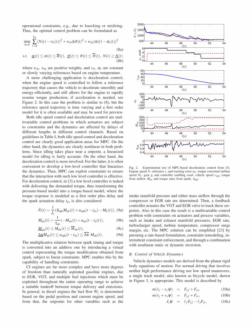
A more challenging application is deceleration control,

when the engine speed is controlled to follow a reference

trajectory that causes the vehicle to decelerate smoothly and

energy-efficiently, and still allows for the engine to rapidly

resume torque production, if acceleration is needed, see

Figure 2. In this case the problem is similar to (8), but the

reference speed trajectory is time varying and a first order

model for it is often available and may be used for preview.

Both idle speed control and deceleration control are mul-

tivariable control problems in which actuators are subject

to constraints and the dynamics are affected by delays of

different lengths in different control channels. Based on

guidelines in Table I, both idle speed control and deceleration

control are clearly good application areas for MPC. On the

other hand, the dynamics are clearly nonlinear in both prob-

lems. Since idling takes place near a setpoint, a linearized

model for idling is fairly accurate. On the other hand, the

deceleration control is more involved. For the latter, it is often

convenient to develop a low-level controller that linearizes

the dynamics. Then, MPC can exploit constraints to ensure

that the interaction with such low level controller is effective.

For deceleration control, in [3] a low level controller is tasked

with delivering the demanded torque, thus transforming the

pressure-based model into a torque-based model, where the

torque response is modeled as a first order plus delay and

the spark actuation delay tds is also considered

N(t) =1

Je

(κspkMair(t)+ uspk(t − tds)−ML(t)), (9a)

Mair(t) =1

τair

(−Mair(t)+ uair(t − td(t)), (9b)

Mair(t)≤ Mair(t)≤ Mair(t), (9c)

∆κMair(t)≤ uspk(t − tds)≤ ∆κ Mair(t). (9d)

The multiplicative relation between spark timing and torque

is converted into an additive one by introducing a virtual

control representing the torque modification obtained from

spark, subject to linear constraints. MPC enables this by the

capability of handling constraints.

CI engines are far more complex and have more degrees

of freedom than naturally aspirated gasoline engines, due

to EGR, VGT, and multiple fuel injections which must be

exploited throughout the entire operating range to achieve

a suitable tradeoff between torque delivery and emissions.

In general, in diesel engines the fuel flow Wf is determined

based on the pedal position and current engine speed, and

from that, the setpoints for other variables such as the

44 46 48 50 52 54500

1000

1500

2000

44 46 48 50 52 540246

44 46 48 50 52 540

15304560

t[s]

t[s]

t[s]

N,r,N

T

gi,

enab

v sp

d

44 46 48 50 52 54−150−100

−500

50100

44 46 48 50 52 540

50100150200250

44 46 48 50 52 540.40.60.8

1

t[s]

t[s]

t[s]

ε NM

air

κsp

k

Fig. 2. Experimental test of MPC-based deceleration control from [3].Engine speed N, reference r, and tracking error εN , torque converted turbinespeed NT , gear gi and controller enabling enab, vehicle speed vspd , torquefrom airflow Mair and torque ratio from spark, κspk .

intake manifold pressure and either mass airflow through the

compressor or EGR rate are determined. Then, a feedback

controller actuates the VGT and EGR valve to track these set-

points. Also in this case the result is a multivariable control

problem with constraints on actuators and process variables,

such as intake and exhaust manifold pressures, EGR rate,

turbocharger speed, turbine temperature, compressor surge

margin, etc. The MPC solution can be simplified [23] by

pursuing a rate-based formulation, constraint remodeling, in-

termittent constraint enforcement, and through a combination

with nonlinear static or dynamic inversion.

B. Control of Vehicle Dynamics

Vehicle dynamics models are derived from the planar rigid

body equations of motion. For normal driving that involves

neither high performance driving nor low speed maneuvers,

a single track model, also known as bicycle model, shown

in Figure 3, is appropriate. This model is described by

m(vx − vyψ) = Fx f +Fxr, (10a)

m(vy + vxψ) = Fy f +Fyr, (10b)

Jzψ = ℓ f Fy f − ℓ jFyr, (10c)

βδ

ψα f

αr

v

ℓ f ℓr

v f

vr

vx f

vy f

vxr

vyr

Fx f

Fy f

x

y

z

Fig. 3. Schematics of single track model of the lateral vehicle dynamics.The relevant vectors for involved are also shown.

where m is the vehicle mass, ψ is the yaw rate, vx, vy are

the components of the velocity vector in the longitudinal and

lateral vehicle direction, Jz is the moment of inertia about the

vertical axis, ℓ f , ℓr are the distances of front and rear axles

from the center of mass. In (10), Fi j, i ∈ {x,y}, j ∈ { f ,r}are the longitudinal and lateral, front and rear tire forces

expressed in the vehicle frame [24],

Fx j = fl(α j ,δ j,σ j,µ ,Fz j), Fy j = fc(α j ,δ j,σ j,µ ,Fz j),

Fz j =ℓ j

ℓ f + ℓr

mg,(11)

where δ j is the steering angle at the tires, α j is the tire slip

angle and σ j is the slip ratio, for front and rear tires j ∈{ f ,r}. The slip angles and the slip ratios relate the tractive

forces with the vehicle velocity and wheel speed, thereby

coupling the vehicle response with the powertrain response,

vl j = vy jsinδ j + vx j cosδ j, vc j = vy j

cosδ j − vx j sinδ j,

α j = tan−1

(

vy j

vx j

)

, σ j =rω j − vx j

max{rω j,vx j,ε}(12)

where vx j, vy j, j ∈ { f ,r}, are the longitudinal and lateral

components of the tire velocity vectors, and ε is a small

constant to avoid singularity. In (11), fl , fc define the tire

forces that are generated as functions of the slip angles and

slip ratio, of the vertical force, and of the friction coefficient

and are in general determined by data or according to a

model such as Paceijka’s formula or Lu’Gre [25].

In the mentioned normal driving conditions, the longi-

tudinal and lateral dynamics are often decoupled, yielding

a lateral dynamics model where vx is constant, and, with

a further linear approximation of the lateral tire forces as

functions of the slip angles resulting in

mvy =−C f +Cr

vx

vy −(

vx −C f ℓ f −Crℓr

vx

)

ψ +C f δ , (13a)

Jzψ =−C f ℓ f −Crℓr

vx

vy −C f ℓ

2f +Crℓ

2r

vx

ψ + ℓ fC f δ +Mbr,

(13b)

where we used α f = (vy + ℓ f ψ)/vx, αr = (vy − ℓrψ)/vx, and

we have included the moment Mbr that can be generated by

applying non-uniform forces at different wheels, for instance

by differential braking. In (13), C f , Cr are the front and

rear lateral tire stiffnesses, which correspond to a linear

approximation of the lateral tire forces as functions of the

slip angles, Fy j =C jα j .

Similarly, the longitudinal dynamics are also simplified by

neglecting the lateral dynamics, resulting in

mvx =Cxf σ f +Cx

r σr −Fres, (14a)

Fres =1

2ρairA f cdv2

x +mgcr cosθrd +mgsinθrd, (14b)

where C f , Cr are the front and rear longitudinal tire stiff-

nesses that represent a linear approximation of the longitu-

dinal tire forces as functions of the slip ratio Fx j =Cxj σ j. The

slip ratio changes based on the torques exerted on the wheels

by the engine and the brakes, thus relating the powertrain and

braking system actuation with the vehicle motion. In (14) we

have included the effects of resistance forces due to airdrag,

rolling, and road grade. Here ρair is the density of air, A f

is the vehicle frontal area, cd is the drag coefficient, θrd is

the road grade, cr is the rolling resistance coefficient, and g

is the acceleration due to gravity. The longitudinal vehicle

dynamics can be linked to the powertrain torque production

in several ways. For low bandwidth applications, such as

cruise control, one can approximate Cxf σ f +Cx

r σr ≈ Ftrac,

where the driveline shafts are assumed to be rigid. The

tractive force applied from the powertrain, to the wheels Ftrac

is the response of a first order-plus-delay system including

a multiplicative factor modeling losses, γls ∈ (0,1),

Ftrac =− 1

τF

Ftrac +γls

τF

uF(t − tF).

If shaft compliance is considered, the tractive torque Mtrac =Ftrac/rw is caused by the slip between the wheel half-shafts

and the rigid transmission shaft, so that

Mtrac = ks(θe −θwgr)+ ds(θe − θwgr), (15)

where ks and ds are the half-shafts stiffness and damping,

θe, θw are the engine and wheel shaft angles, and gr is the

total gear ratio between engine and wheels.

1) MPC opportunities in vehicle dynamics: MPC for

longitudinal vehicle dynamics has been applied to adaptive

cruise control (ACC), see, e.g., [26]. The objective of adap-

tive cruise control is to track a vehicle reference speed r

while ensuring a separation distance d from the preceding

vehicle, related to the head-away time Th, and comfortable

ride, all of which can be formulated as

minFtrac

TN

∑t=0

(vx(t)− rv(t))2 +wF ∆uF(t)

2 (16a)

s.t. F trac ≤ Ftrac(t)≤ F trac, (16b)

d(t)≥ Thvx(t), (16c)

where wF is a positive tuning weight. For ACC, interesting

opportunities are opened when a stochastic description of

the velocity of the traffic ahead is available or can be

estimated [27], or, in the context of V2V and V2I, when there

is perfect preview through communication [19]. Also, using

an economic cost can help reduce fuel consumption, with

minimal impact on travel time [28]. Additional applications

in longitudinal vehicle dynamics that have been explored

but still need to be investigated in depth are launch control

and gear shifting. More recent applications involve braking

control for collision avoidance systems, see, e.g., [29], again,

possibly by using V2X to exploit preview information.

The interest in lateral dynamics spans multiple applica-

tions, especially lateral stability control and lane keeping,

up to autonomous driving. A challenging case [5] is the

coordination of differential braking moment and steering to

enforce cornering, i.e., yaw rate reference rψ tracking, and

vehicle stability, i.e., avoiding that the slip angles become so

large that the vehicle spins out of control. Such a problem is

challenging due to its constrained multivariable nature and

the need to consider nonlinear tire models. A viable approach

is to approximate the tire model as piecewise linear, resulting

in the optimal control problem

min∆δ ,Mbr

TN

∑t=0

(ψ(t)− rψ(t))2 +wδ ∆δ (t)2 +wbrMbr(t)

2 (17a)

s.t. |δ (t)− δ (t − 1)| ≤ ∆δ , |δ (t)| ≤ δ , (17b)

(17c)

|Mbr(t)| ≤ Mbr, |α j| ≤ α j, (17d)

fc j(α j) =

−d jα j + e j if α j > p j,C jα j if |α j| ≤ p j,d jα j − e j if α j <−p j,

(17e)

where wδ , wbr are positive tuning weights, and then using

either a hybrid MPC or a switched MPC, where the current

linear model is applied for prediction during the entire

horizon. Figure 4 shows experimental results in a slalom

tests where MPC controls the slip angles to be near the peaks

where the maximum tire forcs are achieved.

−0.2 −0.1 0 0.1 0.2−0.2

−0.15

−0.1

−0.05

0

0.05

0.1

0.15

0.2

α f [rad]

αr

[rad

]

Fig. 4. Results of MPC control of lateral vehicle dynamics in a in aslalom test on snow. Phase plane plot of the tire slip angles; the dashedlines indicates the angles p j , j ∈ { f ,r} where maximum force is achieved.

As for the vertical dynamics, MPC offers interesting

possibilities for active suspension control when preview of

the road is available [18], [30], for instance obtained from a

forward looking camera.

engine

motorgenerator

battery

fuel vehicle

power

mechanicalmechanicalcoupling

coupling

coupling

electrical

(1)

(2)

(3)

Fig. 5. Schematic of a powersplit HEV architecture. The arrows indicate theallowed power flow directions. The series HEV architecture is obtained byremoving the link (1), thus the mechanical couplings are simply mechanicalconnections. The parallel HEV architecture is obtained by removing thegenerator and hence links (2) and (3).

C. Energy Management in Hybrid Vehicles

The novel element in hybrid powertrains is the presence

of multiple power generation devices, e.g., engine, motor,

generator, and energy storage devices, e.g., fuel tank, battery,

flywheel. The most common hybrid powertrains are hybrid

electric vehicles (HEV) where the internal combustion engine

is augmented with electric motors and generators, and batter-

ies for energy storage. For HEV there are several component

topologies that determine the configurations of the power

coupling, the most common being series, parallel, powersplit,

and electric rear axle drive (ERAD).

The presence of multiple power generation devices re-

quires modeling the power balance. A general model for

the mechanical power balance that ultimately describes the

amount of power delivered to the wheels is

Pveh = Peng −Pgen +Pmot−Plosmec, (18)

where Pveh is the vehicle power for traction, Peng is the

engine power, Pgen is the mechanical power used to generate

electrical energy to be stored in the battery, Pmot is the

electrical power used for traction and Plosmec are the mechanical

power losses. In some HEV architectures, such as the pow-

ersplit architecture in Figure 5, motoring and electric energy

generation can be accomplished by multiple components,

since, despite the names indicating the most efficient usage,

both the motor and the generator can operate in both modes.

The electrical power balance that is used to determine the

power delivered to/from the battery is often modeled as

Pbat = Pmot −Pgen +Plosgen +Plos

mot, (19)

where Pbat is the power flowing from the battery and Plosgen,

Plosmot are the losses in electric energy generation and in the

electric motoring, respectively.

Since, as opposed to the fuel tank, the battery power

flow is bi-directional and the stored energy is usually quite

limited, the energy stored in the battery should be tracked

and it is in fact the main state of the HEV model. The energy

stored in the battery is related to the stored charge, which

is normalized with respect to the maximum to obtain the

battery state of charge (SoC) SoC = QbatQmax

. The battery power,

voltage, and current are related by

Pbat = (V ocbat − IbatRbat)Ibat,

where V ocbat is the open circuit battery voltage, Ibat is the

battery current and Rbat is the battery internal resistance. This

results in the state of charge dynamics

˙SoC =−V oc

bat−√

V ocbat

2 − 4RbatPbat

2RbatQmax.

Considering a power coupling that is under voltage control

and representing the battery as an ideal capacitor, i.e., ignor-

ing internal resistance, we obtain a simpler representation

˙SoC =−ηbat(Pbat,SoC)Pbat

V ccbatQmax

,

where ηbat is the battery efficiency, that, for control purposes

may be approximated by one or two constants [17], the latter

modeling different charging and discharging efficiencies.

The main novel control problem in HEV powertrains is

the management of the energy in order to minimize the fuel

consumption, subject to a charge sustaining constraint

min

∫ t f

ti

Wf (t)dt (20a)

s.t. SoC(ti) = SoC(t f ), (20b)

where the fuel flow Wf is related to the engine power

by a function that depends on the engine operation, Wf =f f (Peng,N). As opposed to conventional powertrains, in most

HEV configurations, even for a given engine power and

wheel speed, there are degrees of freedom in selecting the

engine operating point, i.e., engine speed and engine torque,

that can be leveraged by the energy management strategy.

1) MPC opportunities in hybrid vehicles: Due to the focus

on optimizing the energy consumption subject to constraints

on power flows and battery state of charge, HEV energy

management has been a clear target for MPC application.

The key idea is to construct a finite horizon approximation

of the fuel consumption cost function (20a), augmented with

a term penalizing large differences of SoC at the end of

the horizon, which can be interpreted as the augmented

Lagrangian form of the charge sustaining constraint (20b).

The cost function can also include additional terms such as

SoC reference tracking. Constraints on the various power

flows and battery SoC can also be included, resulting in

minPbat,...

FN(SoC(TN))+TN−1

∑t=0

Wf (t)+wsoc(SoC(t)− rSoC(t))2

s.t. Peng −Pgen+Pmot−Plosmec = Pdrv,

SoC ≤ SoC(t)≤ SoC, |Pbat| ≤ Pbat. (21)

The mechanical power equation (18) is enforced as a con-

straint in (21) to ensure that the vehicle power is equal to

the driver-requested power. The actual degrees of freedom

vary with the HEV architecture. Ignoring the gear shifting

strategy, which is usually separately optimized, for a pow-

ersplit architecture shown in Figure 5 there are two degrees

0.1

0.2

0.2

0.25

0.25

0.28

0.28

0.3 0.305

0.308

0.31

0 2000 4000 60000

50

100

150

200

ζ ∗sys

τ en

g[N

m]

N [RPM]

Lo

Hi

Fig. 6. Distribution of series HEV engine operating points on an experimenton UDDS cycle. Dash green line indicates maximal efficiency operatingpoints for given power output.

of freedom. For a parallel architecture, where there is no

generator, and for a series architecture, where there is no pure

mechanical connection between engine and wheels, there is

one degree of freedom. Exploiting the simplicity of the latter,

an MPC was developed in [17] which was deployed on a

fully functional, production-prototype, series HEV that was

also road driven, see Figure 6.

In recent years several advanced MPC methods have been

applied to HEV energy management, including stochastic

MPC [31] where the driver-requested power is predicted

using statistical models learned from data during vehicle

operation [32].

IV. AEROSPACE APPLICATIONS AND MODELS

MPC and RTO have been extensively investigated for

aerospace control applications, see for instance the sur-

vey [33], and [34] and the accompanying special issue

of AIAA Journal of Guidance, Dynamics and Control that

introduce computational guidance and control as a paradigm

shift in aerospace control applications.

In aircraft, MPC has been of interest as an advanced

solution for control of gas turbine engines [35], [36] as

these have many constraints, including high pressure and

low pressure compressor surge/stall margins, core and fan

over speed limits, over temperature limits, lean combustion

blowout limits, etc. MPC solutions have also been considered

for integrated thrust and electrical power delivery in more

electric aircraft, see e.g., [37]. One of the current frontiers

for the use of MPC is maneuver and gust load alleviation for

flexible aircraft [38]. In these applications, MPC solutions

must accommodate high order models resulting from finite

element or modal analysis, multiple control effectors, lack

of full state measurement, gust disturbances, and be feasible

for implementation at high sampling rates.

In spacecraft control, many RTO applications have been

considered. In particular, advanced solutions for powered

descent and landing based on real-time convex optimization

and ideas of lossless convexification has been developed

and flight tested [39]–[43]. A challenging application to

combined station-keeping and momentum-management to

enable future Earth-Moon halo orbit tracking missions has

been considered in [44]. Next, we provide an introductory

overview of some of the relevant models and of the control

problems that can be addressed by MPC in such applications.

A. Control of Spacecraft Attitude

Spacecraft attitude control involves control of spacecraft

orientation. Suppose the spacecraft orientation relative to an

inertial frame is specified by 3-2-1 Euler angles φ (roll),

θ (pitch), and ψ (yaw). Assuming the spacecraft bus fixed

frame is a principal frame, the spacecraft attitude kinematics

and dynamics equations are given by

φθψ

=

cos(θ ) sin(φ)sin(θ ) cos(φ)sin(θ )0 cos(φ)cos(θ ) −sin(φ)cos(θ )0 sin(φ) cos(φ)

× 1

cos(θ )

ω1

ω2

ω3

, (22a)

J1ω1 +(J3 − J2)ω2ω3

J2ω2 +(J1 − J3)ω1ω3

J3ω3 +(J2 − J1)ω1ω2

=−

M1

M2

M3

, (22b)

where ω1, ω2, ω3 are components of angular velocity vector

expressed in spacecraft body fixed frame. The state vector

is six dimensional, X = [φ θ ψ ω1 ω2 ω3]′, and the control

vector, which encompasses components of control moment,

has the form, U =[

M1 M2 M3

]′.

1) MPC opportunities in attitude control: For attitude

control, MPC allows to enforce constraints, from simple

torque actuator constraints |Mi| ≤ Mi, i = 1, . . . ,3, to in-

clusion zone constraints, fizn(θ ,φ ,ψ) ∈ I , modeling, for

instance, requirements to maintain Line-of-Sight, and ex-

clusion zone constraints, fxzn(θ ,φ ,ψ) /∈ E , modeling, for

instance, requirements to avoid exposure of instruments to

high energy/radiation sources, e.g., the sun.

For applying linear MPC, the attitude dynamics can be lin-

earized around the origin resulting in three uncoupled double

integrators about each of three individual axes. Appropriate

choices of the sampling period are in the order of a fraction

of a second to several seconds, depending on the agility of

the spacecraft and the target maneuvers. The closed-loop

response of a basic MPC with a nonlinear attitude model

is shown in Figure 7.

The basic design can be extended in several directions.

In [45] a spacecraft with reaction wheel actuators is consid-

ered, and a special formulation of the cost with the virtual

reference is exploited to expand the closed-loop domain

of attraction, along with a low complexity addition of the

integral action performed at the reference and outside of

MPC controller, to guarantee offset-free tracking of attitude

set points. A dual projected gradient algorithm which is

suitable for implementation in fixed point arithmetic is

applied to solve online the resulting quadratic program

Fig. 7. The time histories of Euler angles and control moments.

(QP). In another extension, [46], MPC is used to implement

reaction wheel desaturation maneuvers through either gravity

gradients or magnetic torquers while maintaining spacecraft

pointing within specified constraints. The treatment involves

modifying spacecraft model with reaction wheel states and

adding gravity gradient and magnetic actuation effects.

Another interesting opportunity is based on the fact that a

globally stabilizing control law for attitude control must be

discontinuous, due to the topological properties of SO(3).However, nonlinear MPC can result in discontinuous feed-

back policies, and in [47] it was shown that SO(3)-based

MPC can globally stabilize the spacecraft attitude.

B. Control of Spacecraft Relative Motion

Spacecraft relative motion control refers to the control

of spacecraft motion (translational or both translational

and rotational) relative to a nominal orbital position as

required by missions involving, e.g., rendezvous, docking,

proximity operations, circumnavigation, orbit adjustment or

maintenance. While in the past spacecraft translational and

orbital transfer problems have been addressed by open loop

maneuver planning and optimal control techniques, recent

interest in MPC has been strongly motivated by MPC ability

to deal with various constraints such as thrust limits, Line-

of-Sight (LoS) cone, soft landing and obstacle avoidance,

while improving robustness to modeling errors. Applications

of MPC to relative motion control have been summarized in

a recent tutorial [48]. Some predictive control solutions have

been tested in-orbit, e.g. for PRISMA mission or developed

for missions around other planets [49].

Hill-Clohessy-Wiltshire (HCW) equations prescribe the

spacecraft relative coordinates in the so called Hill’s (or

local vertical, local horizontal LVLH) frame attached to the

nominal orbital position (see Figure 8). For circular orbits

the HCW equations are time-invariant and are linearized as

x− 3n2x− 2ny =Fx

mc

, (23a)

y+ 2nx =Fy

mc

, (23b)

z+ n2z =Fz

mc

, (23c)

where n is the nominal orbital rate, (x,y,z) are spacecraft

relative coordinates in LVLH frame, mc is the mass of

spacecraft, and Fx, Fy and Fz are thrust forces. Alternatively,

if an impulsive thrust approximation is made, the thrust

Fig. 8. Motion in ECI frame and motion in the relative (LVLH) frame.

Fig. 9. Open-loop and MPC-based relative motion maneuvers.

forces can be replaced by velocity changes as inputs [11].

The in-orbital plane dynamics (x,y) are decoupled from

the out of the orbital plane dynamics z, and there is an

asymmetry in the dynamics between x (radial or R-bar)

direction and y (in orbital track or V-bar) direction.

1) MPC opportunities in relative motion control: For

spacecraft relative motion control, MPC provides increased

robustness against model error and perturbances. Figure 9

illustrates how an open-loop maneuver computed based

on (23) misses the target when simulated on the nonlinear

model. However, MPC reaches the target by recomputing the

solution in a receding horizon manner.

For spacecraft docking, the implementation of MPC ben-

efits from decomposing the maneuver into two phases, a

rendezvous phase and a docking phase with different cost

functions and constraints [11]. In rendezvous phase, LoS

cone constraints are not applied and, to increase the domain

of attraction, the spacecraft position is controlled to a virtual

set-point, the difference of which and the target is also

penalized in the cost. In the docking phase, activated when

the spacecraft is sufficiently close to the target, LoS, thrust

direction, and soft docking constraints are imposed, and

the virtual set-point is removed. The thrust constraints are

imposed in both phases of the maneuver. Figure 10 illustrates

a typical maneuver resulting from such a decomposition.

The requirements of more complex missions that involve

avoiding debris or docking to rotating targets can be ad-

dressed by dynamically reconfiguring the constraints during

the maneuver [10]. For instance, a nonconvex constraint of

avoiding a debris can be handled by separating the spacecraft

from a debris by a rotating hyperplane [10], [11]. This avoids

the need for integer variables as in [50], and results in an

optimization problem that at each stage is a convex QP.

Fig. 10. Spacecraft maneuver with rendezvous and docking phases andLoS cone constraints.

The experimental testing of relative motion maneuvers is

feasible in simple robotic testbeds where distance and time

scaling is used to map the motion in orbital plane to the

motion of the ground robots on the floor [51]. More complex

test beds have been also developed such as POSEIDYN [52].

C. Spacecraft motion control near an asteroid or a comet

The spacecraft control near a small body (an asteroid or a

comet) are involved due to the uncertainty of the gravitation

field and other effects such as comet outgassing pressure that

are difficult to characterize in advance of the mission. At the

same time, given that the small body forces are relatively

weak, MPC-based feedback control can be very effective

in robustifying spacecraft maneuvers to the uncertainties in

small body environment.

The relative motion of a spacecraft in an asteroid fixed

frame is described by [53],

x = Fg,x + 2ny+ n2x+ ux,y = Fg,y − 2nx+ n2y+ uy,

z = Fg,z + uz,

where n is the rotation rate of the asteroid, Fg,x, Fg,y and

Fg,z are the components of the gravitational force per unit

mass exerted on the center-of-mass of the spacecraft by the

asteroid, and ux, uy, and uz are the control inputs which

correspond to thrust induced accelerations. The gravity force

is computed from the potential, given as a summation of

spherical harmonics,

G =− µ

R0

∞

∑l=0

n

∑m=0

(Cl,mVl,m + Sl,mWl,m),

where µ is the asteroids gravitational constant, R0 is the

radius of a reference sphere, Cl,m and Sl,m are the Stokes

coefficients, and Vl,m and Wl,m are functions of position cal-

culated using the Montenbruck recursion scheme [54]. The

gravity force is the gradient of the potential [Fg,x Fg,y Fg,z]′ =

−∇G. Taking ξ = [ x y z x y z ]′ = [r′ v′]′ as the relative

state vector, and u = [ ux uy uz ]′ as the control vector, the

equations of motion can be as affine-in-controls,

ξ (t) = Acξ (t)+Fg(ξ (t))+Bcu(t).

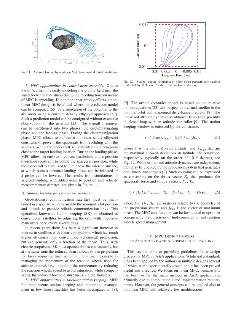
Fig. 11. Asteroid landing by nonlinear MPC from several initial conditions.

1) MPC opportunities in control near asteroids: Due to

the difficulties in exactly modeling the gravity field near the

small body, the robustness due to the receding horizon nature

of MPC is appealing. Due to nonlinear gravity effects, a non-

linear MPC design is beneficial where the prediction model

can be computed [55] by a truncation of the potential to the

4th order using a constant density ellipsoid approach [53].

Such a prediction model can be configured without extensive

observations of the asteroid [55]. The overall maneuver

can be partitioned into two phases, the circumnavigating

phase and the landing phase. During the circumnavigation

phase, MPC allows to enforce a nonlinear safety ellipsoid

constraint to prevent the spacecraft from colliding with the

asteroid, while the spacecraft is controlled to a waypoint

close to the target landing location. During the landing phase,

MPC allows to enforce a convex paraboloid and a position

overshoot constraint to bound the spacecraft position, while

the spacecraft is stabilized to 2 m above the asteroid surface,

at which point a terminal landing phase can be initiated or

a probe can be lowered. The results from simulations of

asteroid landing, with added noise to position and velocity

measurements/estimates, are given in Figure 11.

D. Station keeping for Low thrust satellites

Geostationary communication satellites must be main-

tained in a specific window around the nominal orbit position

and attitude to provide reliable communication links. This

operation, known as station keeping (SK), is obtained in

conventional satellites by adjusting the orbit with impulsive

maneuvers once every several days.

In recent years there has been a significant increase in

interest in satellites with electric propulsion, which has much

higher efficiency than conventional (chemical) propulsion,

but can generate only a fraction of the thrust. Thus, with

electric propulsion, SK must operate almost continuously, but

at the same time the reduced thrust allows to use propulsion

for tasks requiring finer actuation. One such example is

managing the momentum of the reaction wheels used for

attitude control, i.e., unloading the momentum by reducing

the reaction wheels speed to avoid saturation, while compen-

sating the induced torque disturbances via the thrusters.

1) MPC opportunities in satellites station keeping: MPC

for simultaneous station keeping and momentum manage-

ment in low thrust satellites has been investigated in [8],

Longitude Error (deg)

Lat

itude

Err

or

(deg

)

-0.01-0.00500.0050.01

-0.01

0

0.01

Fig. 12. Station keeping simulation of a low thrust geostationary satellitecontrolled by MPC over 5 orbits. SK window in dash red.

[9]. The orbital dynamics model is based on the relative

motion equations (23) with respect to a virtual satellite in the

nominal orbit with a nominal disturbance predictor [8]. The

linearized attitude dynamics is obtained from (22), possibly

in closed-loop with an attitude controller [9]. The station

keeping window is enforced by the constraints

|y| ≤ r tan(λlong), |z| ≤ r tan(λlat), (24)

where r is the nominal orbit altitude, and λlong, λlat are

the maximal allowed deviations in latitude and longitude,

respectively, typically on the order of 10−2 degrees, see

Fig. 12. While orbital and attitude dynamics are independent,

they may be coupled by the propulsion system that generates

both forces and torques [9]. Such coupling can be expressed

as constraints on the thrust vector Fth that produces the

spacecraft force and torque vectors, Fsc, Tsc,

0 ≤ HthFth ≤ fmax, Tsc = DT Fth, Fsc = DF Fth. (25)

where DT , DF , Hth, are matrices related to the geometry of

the propulsion system and fmax is the vector of maximum

thrust. The MPC cost function can be formulated to optimize

concurrently the objectives of fuel consumption and reaction

wheels speed management.

V. MPC DESIGN PROCESS

IN AUTOMOTIVE AND AEROSPACE APPLICATIONS

This section aims at providing guidelines for a design

process for MPC in A&A applications. While not a standard,

it has been applied by the authors in multiple designs several

of which were experimentally tested, and it has been proved

useful and effective. We focus on linear MPC, because this

has been so far the main method in A&A applications,

primarily due to computational and implementation require-

ments. However, the general concepts can be applied also to

nonlinear MPC with relatively few modifications.

We consider the finite horizon optimal control problem

minU(t)

x′N|tPxN|t +N−1

∑k=0

z′k|t Qzk|t + u′k|tRuk|t (26a)

s.t. xk+1|t = Axk|t +Buk|t , (26b)

yk|t =Cxk|t +Duk|t , (26c)

zk|t = Exk|t , (26d)

uk|t = κ f xk|t , k = Nu, . . . ,N − 1, (26e)

x0|t = x(t), (26f)

y ≤ yk|t ≤ y, k = Ni, . . .Ncy, (26g)

u ≤ uk|t ≤ u, k = 0, . . .Ncu − 1, (26h)

HNxN|t ≤ KN , (26i)

where the notation k|t denotes the k-steps prediction from

measurements at time t, U(t) = {u0|t . . .uN−1|t}, x,u,y,z are

the prediction model state, input, constrained outputs, and

performance output vectors, u,u,y,y are lower and upper

bounds, P,Q,R are weighting matrices, N,Ncu,Ncy,Nu are

non-negative integers defining the horizons, κ f is the ter-

minal controller, and HN ,KN define the terminal set.

The MPC design amounts to properly constructing compo-

nents of the finite horizon optimal control problem to achieve

the desired specifications and control-oriented properties, as

we discuss next.

A. Prediction Model

Several A&A processes are well studied and have readily

available models, some of which have been described in

Sections III, IV. In MPC design it is desirable to start from

such physics oriented models. However many of them may

be of unnecessarily high order, may be nonlinear, and may

require estimation of several parameters. Hence, usually the

first step in MPC design is to refine the physics based model

by:

• simplifying the model to capture the relevant dynamics

for the specific application and controller requirements,

by linearization, model order reduction, etc;

• estimating the unknown parameters by gray-box system

identification methods, e.g., linear/nonlinear regression,

step response analysis, etc.;

• time-discretizing the dynamics for use in a discrete-time

prediction model.

Even for the simple case of idle speed control, in [2] due

to computational requirements, the powertrain model (1), (4),

(5) is linearized around the nominal idle operating point, with

the models for the delays removed during identification, to be

added again later. The model structure is known from physics

and the parameters are identified from step responses.

The result of such first model construction step is a linear

discrete-time model for the process,

xm(t + 1) =Amxm(t)+Bmum(t), (27a)

ym(t) =Cmxm(t)+Dmum(t), (27b)

zm(t) =Emxm(t), (27c)

where xm ∈ Rnm is the state vector, um ∈ R

mm is the input

vector ym ∈ Rpm is the constrained output vector, and zm ∈

Rqm is the performance output vector.

The process model (27) usually needs to be augmented

with additional states and artificial dynamics in order to

achieve the problem specifications, such as tracking of

references, non-zero and possibly unknown steady state

input values, rejection of certain classes of disturbances.

Further modifications may be made to account for additional

information available in the system, such as preview on

disturbances or references, or known disturbance models.

Typical augmentations are the incremental input formulation

u(t + 1) = u(t)+∆u(t),

the inclusion of integral action to track constant references

and reject constant unmeasured disturbances,

ι(t + 1) = ι(t)+TsCι z(t),

and the inclusion of disturbance models

η(t + 1) = Aη(t),

d(t) = Cdη(t),

where the disturbance model state η is measured in the case

of measured disturbances, while in the case of unmeasured

disturbance it is estimated from disturbance observers. A case

of particular interest is the inclusion of buffers to account for

time delays and preview on disturbances and references,

ξ (t + 1) =

[

0 I

0 c

]

ξ (t),

χ(t) =[

1 0 . . . 0]

ξ (t),

where c is usually either 1 or 0 depending on whether the

last value in the buffer is to be held constant or set to 0. An

exact linear model of the delay buffer can be formulated only

in discrete-time, while in continuous-time one must resort

to Pade approximations that may introduce fictitious non-

minimum phase behaviors and mislead the control decisions.

Due to its intrinsic feedforward-plus-feedback nature,

MPC is often applied for reference tracking. However, the

application of MPC to these problems is not as simple as

for linear controllers, because the constraints usually prevent

from simply “shifting the origin”. In some applications, it

may be difficult, to compute the equilibrium associated with

a certain reference value r due to the uncertainty of the

model and the unmeasured disturbances. If one wants to

avoid adding a disturbance observer, it may be effective to

apply the velocity (or rate-based) model form [23], where

both the state and input are differentiated, and the tracking

error em is included as an additional state,

∆xm(t + 1) =Am∆xm(t)+Bm∆um(t), (28a)

em(t) =em +Em∆xm(t)+∆r(t), (28b)

ym(t) =ym(t − 1)+Cm∆xm(t)+Dm∆um(t), (28c)

where ∆r is the change in reference value. For MPC appli-

cations one may need to add integrators to compute ym from

Specification Model Augmentation

Piecewise constant reference or measured disturbance Incremental inputMeasured non-predictable disturbance Constant disturbance modelPreviewed reference/disturbance Preview reference/disturbance bufferKnown time delay Delay bufferUnmeasured constant disturbance Output/tracking error integral action, Output disturbance and observerReference tracking Reference model and tracking error, velocity form

TABLE II

LIST OF COMMON SPECIFICATIONS AND RELATED AUGMENTATIONS TO THE PROCESS MODEL TO HANDLE THEM.

the state and input changes, ∆xm, ∆um, except for the cases

where the constraints are originally in differential form.

The more common augmentations in relations to specifi-

cations usually found in A&A applications are summarized

in Table II. Applying all the augmentations result in a higher

order prediction model (26b)–(26d),

xk+1|t = Axk|t +Buk|t , x =

[

xm

xp

]

, u =

[

um

up

]

, (29a)

yk|t =Cxk|t +Duk|t , y =

[

ym

yp

]

, (29b)

zk|t =Exk|t , z =

[

zm

zp

]

, (29c)

where x ∈ Rn, u ∈ R

m, y ∈ Rp, z ∈ R

q are the prediction

model state, input, constrained outputs, and performance

output vectors, xp,up,yp,zp are the ancillary state, input,

constrained outputs, and performance output vectors.

B. Horizon and Constraints

The constraints are usually enforced on the constrained

output vector and on the input. While enforcement of the

constraints directly on the states is certainly possible, it is

more convenient to introduce the constrained output vector y

specifically for this use, which allows to enforce state, mixed

state-inputs, and also pure input constraints through a single

vector. Thus, the constraints may be formulated as

yk|t ∈ Ym, uk|t ∈ Um, (30)

where and Ym and Um are the admissible sets for constrained

output and input vectors, respectively. Enforcing constraints

on the constrained output and input vectors of the predic-

tion model, which include augmentation, usually allows to

formulate (30) as simple bounds in (26g), (26h),

y ≤ yk|t ≤ y, u ≤ uk|t ≤ u, (31)

which are easier to specify and handle in the optimization.

In A&A applications, the sampling period Ts of the pre-

diction model (29) is often equal to the period of the control

cycle for the function being developed. However, for (29)

to be accurate, Ts should be small enough to allow for 3-10

steps in the settling of the fastest dynamics, following a step

response. If this is not the case, upsampling or downsampling

may be advised, where the prediction model sampling period

and the control loop period are different, and appropriate

strategies, such as move blocking or interpolation, are applied

to bridge such differences.

The choice of the prediction horizon N is related to the

prediction model dynamics. In general, N should be slightly

larger, e.g., 1.5×-3×, than the number of steps for the

settling of the slowest (stable) prediction model dynamics,

following a step response. This requirement relates to the

choice of the sampling period so that the total amount

of prediction steps is expected to be 5-30 times the ratio

between the slowest and the fastest (stable) system dynamics.

More correctly, the relevant settling time for the choice of the

prediction horizon is that of the closed-loop system, which

usually leads to an iterative selection procedure.

Other horizons can be considered, for adjusting the com-

putational requirements in solving the MPC problem. The

control horizon Nu determines the number of control steps

left as free decision variables to the controller, where for

k ≥ Nu the input is no longer an optimization variable, but

rather assigned by the pre-defined terminal controller (26e),

uk|t = κ f xk|t , k = Nu, . . . ,N − 1. (32)

The constraint horizons, for outputs and inputs, Ncy,Ncu,

respectively, determine for how many steps the constraints

are enforced,

y ≤ yk|t ≤ y, k = Ni, . . .Ncy, u ≤ uk|t ≤ u, k = 0, . . .Ncu −1,(33)

where Ni = {0,1} depending on whether output constraints

are enforced or not at the initial step, which is reasonable

only if the input directly affects the constrained outputs. By

choosing Nu, one determines the number of optimization

variables, nv =Num and by choosing Ncy,Ncu, one determines

the number of constraints, nc = 2(p(Ncy + 1−Ni)+mNcu).This determines the size of the optimization problem. Move

blocking, which allows the input to change only at a subset

of the sampling instants in the prediction horizon, can also

be used to reduce the number of decision variables.

C. Cost Function, Terminal Set and Soft Constraints

The cost function determines the objectives of MPC, and

their priority. To construct that, the control specifications are

converted into variables that are to be controlled to 0. Such

variables are either a part of the process model (27), or are

included in the prediction model (29) by the augmentations

in Section V-A. In general the MPC cost function (26a) is

JN|t = x′N|t PxN|t +N−1

∑k=0

z′k|tQzk|t + u′k|tRuk|t , (34)

Specification Corresponding weights

Regulation/Tracking error Weight on plant output errorEnergy Weight on plant inputNoise, vibration, Weight on plant output acceleration,and harshness (NVH) and plant input rate of changeConsistency Weight on plant output velocity,

and plant input rate of changeComfort Weight on plant output acceleration,

and jerk, and plant input rate of change

TABLE III

LIST OF “DOMAIN TERMS” SPECIFICATIONS AND WEIGHTS THAT OFTEN

AFFECT THEM.

where the performance outputs of the prediction model z =Ex can model objectives such as tracking z = Cx −Crxr,

where xr is the reference model state, and r =Crxr is the cur-

rent reference. In (34), Q ≥ 0, R > 0 are the matrix weights

that determine the importance of the different objectives: for

a diagonal weight matrix Q, the larger the ith component,

the faster the ith performance output will be regulated to 0.

It is important to remember that weights determine relative

priorities between objectives. Hence, increasing the jth per-

formance output weight may slow down the regulation of the

ith performance output.

Very often, the control specifications are given in terms of

“domain quantities”, such as comfort, NVH (noise, vibration,

harshness), consistency, i.e., repeatability of the behavior,

and it is not immediately clear how to map them to corre-

sponding weights. While the mapping tends to be application

dependent, some of the common cases are reported in

Table III, where we stress that the outputs and inputs, and

their derivatives, refer to the plant outputs, which may be

part of the performance outputs or inputs, depending on the

performed model augmentations.

In (34), P≥ 0 is the terminal cost, which is normally used

to guarantee at least local stability. There are multiple ways

to design P. The most straightforward and more commonly

used in A&A applications is to choose P to be the solution of

the Riccati equation, constructed from A, B in the prediction

model (29), and Q, R in the cost function (34),

P = A′PA+Q−A′PB(B′PB+R)−1B′PA.

This method can be used, after some modifications, also

for output tracking [56]. Alternative approaches are based

on the solution of the Lyapunov equation for systems that

are asymptotically stable, or on the solution of an LMI

to determine a stabilizing controller and the corresponding

closed-loop Lyapunov function. The terminal controller u =κ f x used after the end of the control horizon is then chosen

accordingly, being either the LQR controller, constantly 0,

or the stabilizing controller, respectively.

The use of terminal set constraint (26i) to guarantee

recursive feasibility and stability in the feasible domain of the

MPC optimization problem has seen a limited use in A&A

applications. This is mainly due to the many disturbances and

modeling errors acting on the prediction model, which may

cause infeasibility of such constraint, due to the need to keep

the horizon short because of computational requirements.

Instead, for ensuring that the optimization problem admits

a solution, constraint softening is often applied. A QP with

soft constraints can be formulated as

minv,s

1

2v′Hv+ρs2 (35a)

s.t. Hv ≤ K +Ms, (35b)

where s is the slack variable for softening the constraints, M

is a vector of 0 and 1 that determines which constraints are

actually softened, and ρ is the soft penalty, where usually

ρI ≫ Q. In general, only output constraints are softened,

because input constraints should always be feasible for a

well-formulated problem. More advanced formulations with

multiple slack variables giving different priorities to different

constraints are also possible, as well as different weighting

functions for the constraint violation.

While in general one may want to have ρ extremely large

to better emulate hard constraints, this may end up worsening

the problem conditioning with the result that the solution

time increases, and the solution quality may also decrease.

VI. COMPUTATIONS AND NUMERICAL ALGORITHMS

As discussed in Section II, a key challenge for implement-

ing MPC is accommodating its significantly larger computa-

tional footprint when compared to standard controllers, i.e.,

PID. As MPC is based on a solution to a finite time optimal

control problem, the MPC code is significantly more com-

plex, and it may involve iterations, checking of termination

conditions, and sub-routines, as opposed to integrator and

derivative updates, and a “one-shot” computation of the three

terms in the PID feedback law.

The embedded software engineers that are ultimately

responsible for controller deployment need to face this

additional complexity, and need to move from considering

a controller that evaluates a function, to a controller that

executes an algorithm. Furthermore, cost is a key driver in

the automotive and aerospace development. Engineers often

consider advanced control methods as a pathway to reducing

the cost of sensors and actuators, while still achieving

robustness and efficiency through software. If the control

algorithms are so complex that they require the development

of new computational platforms, their appeal is significantly

reduced. Hence, the control developers should always strive

to fit the controller in the existing computational hardware,

rather than assume that computer hardware will become

available that is able to execute it.

The common practice found in many research papers of

extrapolating the real-time behavior of MPC in an automo-

tive/spacecraft micro-controller unit (aMCU/sMCU) from the

one that is seen in a desktop CPU (dCPU) is potentially very

misleading as xMCUs and dCPUs have significantly different

capabilities, see Table IV. First, one needs to consider that

powerful xMCUs usually run more than ten feedback loops,

and probably an even larger number of monitoring loops,

and hence the actual computation power available for a

Freq. Instr./s RAM ROM

dCPU 1000s MHz 100s GIPS 10s GB 1000s GB

aMCU 100s MHz 1000s MIPS 1000s kB 10s MB

sMCU 1000s MHz 10s GIPS 100s MB 1000s MB

TABLE IV

COMPARISON OF COMMON CHARACTERISTICS FOR DESKTOP

PROCESSORS (DCPU), AUTOMOTIVE (AMCU) AND SPACECRAFT

(SMCU) MICRO-CONTROLLERS.

single controller is only a fraction of what is available in the

entire xMCU. The difference between instruction sets (RISC

vs CISC) and the simpler structure of the xMCU memory

architecture results in a significantly different numbers of

instructions per seconds (IPS) for the xMCUs with respect

to dCPUs.

For aMCUs, most of the differences are due to the need

to work in extreme environments, e.g., temperature range

between −40oC and +50oC, in which a dCPU is not required

to operate, and may be even prevented from starting in such

conditions. This is also the cause of the major differences in

the size of execution memory, which is normally DRAM in

dCPU, but is in general permanent (e.g., SRAM, EPROM,

or Flash) in aMCU, with higher cost and physical size, and

hence lower quantities and speeds. In fact, for several embed-

ded platforms, memory access is actually the bottleneck [57].

For sMCUs, while more powerful computing hardware is

permissible for some aerospace systems, such as communi-

cation satellites, the considerations of weight and electrical

power consumption often restrict the available onboard com-

puting power. Such weight constraints are particularly severe

for smaller electric battery powered vehicles, e.g., flapping

wing aircraft or smaller UAVs. The restrictions due to the

need to operate in harsh environments become even more

significant in aerospace applications, due to temperature

that can range between −200oC and +400oC degrees, and

presence of harmful radiations requiring specific processes

of radiation-hardening.

Because of this, and since also processor-specific code

optimization by the engineers or by the custom compilers,

may play a very significant role, the evaluation of the

computational load of an MPC controller in an xMCU can

only be extrapolated by (in order of precision)

• computing the worst case number of operations per type,

the number of instruction per operation type, and hence

the total number of instructions per controller execution,

• executing the controller on the specific platform, com-

puting the cost per iteration, and estimating the allowed

number of iterations per sampling period,

• evaluating the execution time in a dCPU, estimating the

ratio of IPS between dCPU and xMCU, and using that

to estimate the execution time in xMCU.

However, according to Table IV, what is often restricting

is the memory, both for execution and data. Hence the

memory occupancy of the controller is something to be

very mindful of. Indeed, PIDs need a minimal amount of

memory, 3 gains, 2 extra variables for integral and derivative

error, and very few instructions. MPC requires significantly

more memory than PID and hence a careful choice of the

numerical algorithm is often critical to the success of the

application. Based on the previous discussions, algorithms

with limited memory usage and relatively simple code may

be preferred, at least initially.

A. Explicit MPC

Explicit MPC has had a significant impact on the im-

plementation of the first MPC solutions in vehicles. Some

examples, tested in fully functional and road-drivable (and

in several cases road-driven) vehicles are in [2], [3], [5]–

[7], [17], [26], [58]–[60]. For spacecraft attitude control, due

to decoupled form and symmetry of (22b), explicit MPC is

advantageous in terms of memory and computations, and

in [10] explicit MPC for relative motion was developed.

In explicit MPC, the optimizer of (26) is obtained by

evaluating a pre-computed piecewise affine function of the

prediction model state (29),

umpc(x) =

F1x+G1 if H1x ≤ K1,...

Fsx+Gs if Hsx ≤ Ks,

(36)

where s is the total number of regions.

The main advantages of explicit MPC and the reasons for

its appeal in A&A applications are:

• Simple execution code: explicit MPC is a lookup table

of affine controllers, selected by linear inequalities.

• Basic operations: the controller implementation requires

only sums, multiplications, and comparisons.

• Predictability: the worst case number of operations is

simple to compute.

Additional benefits include the possibility of computing

explicit MPC, with few modifications, also for switched

and hybrid systems, which allowed for the application of

switched and hybrid MPC in automotive control [5]–[7],

[26], [58], [59], the possibility of constructing the closed-

loop dynamics and hence to analyze its local and global

stability, and the possibility of storing only the most useful

regions, while resorting to a backup controller otherwise,

thus reducing memory requirements.

On the other hand the explicit MPC data memory occu-

pancy and worst case number of operations grows propor-

tionally to the number of active sets of constraints nas, and

hence exponentially with the number of constraints/variables,

nas ≤min{nc,nv}

∑h=0

(

nc

h

)

, (37)

where nv is the number of variables, and nc is the number

of constraints. Because of (37), explicit MPC is limited

to applications with a relatively short horizon, few control

inputs, and few constraints. Another limitation is that the

construction of (36) is often too complex to be implemented

in micro-controllers, and hence explicit MPC cannot be

easily tuned or changed after deployment.

B. Online MPC

Due to (37), In problems with many control inputs, long

prediction horizons and many constraints, explicit MPC is

be too complex to compute or to store for real-time usage.

Also, if the prediction model changes over time, it is very

difficult to adjust the explicit solution, while it is relatively

simple to update the data of the optimal control problem. In

these cases, the online solution of (26) may be preferable.

Among such cases, in [4], a QP solver and a nonlinear

solver were used online for control of autonomous vehicles,

and this enabled using a long horizon to take maximum

advantage of the known reference trajectory. The nonlin-

ear solver was based on sequential quadratic programming

(SQP), and both the nonlinear and QP solvers used active-

set methods. In [61] an active-set solver was used to solve

QPs for controlling manifold pressure and airflow in a diesel

engine using EGR and VGT. The solver was chosen due

to the many constraints imposed by the problem, and the

need to update the matrices of the model depending on

the current operating point, i.e., using in fact a linear-

parameter varying model of the diesel engine. In [62], due

to the need for using a relatively long horizon for vehicle

dynamics cornering performance and stability control at the

limit of performance, an interior-point solver was used.

While the solvers have been tested in real vehicles, the

computing platforms were dedicated rapid prototyping units

and custom micro-controllers that may be more capable than

production aMCU, in particular, because they are dedicated

to the controller being developed, while aMCUs run multiple

controllers.

Active-set and interior-point methods have fast conver-

gence, but they often use linear algebra libraries for solving

systems of linear equations at each iteration of the opti-

mization. Using these libraries may require a significant

amount of both data and execution memory, and achieving

portability of the libraries to micro-controllers may not be

straightforward. Alternatively, first-order methods may have

slower convergence, but have much simpler code and hence

require less memory and do not require additional libraries.

First order methods are essentially based on updating the

current solution z(h)s in the direction indicated by a function

hs of the gradient of the cost function J with a stepsize αs,

followed by projection onto the feasible set F

z(h+1)s = z

(h)s −αs(z

(h)s ) ·hs

(

d

dzs

J(zs)

∣

∣

∣

∣

z(h)s

)

, (38a)

z(h+1)s = projF

(

z(h+1)s

)

, (38b)

where zs may contain additional variables with respect to

those in the original optimization problem, and the choice

of the stepsize αs, of the function hs, and of the additional

variables differentiate the methods.

In recent years, several first-order methods for MPC have

been proposed, based on Nesterov’s fast gradient algo-

rithm [63], [64], Lagrangian methods [65], nonnegative least

squares [66], and alternating direction method of multipli-

ers [67]–[69]. For instance, in [70] the method in [66] was

used for vehicle trajectory tracking.

Another advantage of first order methods is that, due to

their simple structure, it is often possible to derive a worst

case number of iteration [63], [64]. This allows to “size” the

processor to the optimization algorithm. On the other hand in

many real A&A applications, the processor is already fixed

at the time the control algorithm is designed. Hence, it may

be even more effective to use algorithms that allow for early

termination while still providing some guarantees, at least

with respect to constraint satisfaction, such as, for instance,

primal active set methods [71].

C. Nonlinear MPC

Most of the previous discussion is focused on linear MPC

because, at least until very recently, that was the only class of

MPC that could have been realistically implemented in most

A&A systems. Nonlinear MPC (NMPC) is significantly more

complex, which is to a large extent due to the algorithm for

solving the nonlinear programming problem. For instance,

in [4] the authors after implementing a nonlinear method,

chose to implement a linear time-varying method based on

local linearization and quadratic programming, to reduce

the computational load. As another example, [72] concerned

with diesel engine air path control states that “currently it

is not possible to implement NMPC in real time due to

the limited computational power available.” However, this

is starting to change in more recent years, in part thanks to

the research aimed at tailoring nonlinear solvers to MPC.

For spacecraft control near an asteroid, in [55] the nonlin-

ear optimization problem in NMPC, is solved by a nonlinear

primal dual filter-line search interior point solver. Sensitivity

based warm-starts are used to reduce the computational

burden of the algorithm by taking advantage of information

from previous solutions, which is based on the receding

horizon nature of MPC. It shall be noted however that, if

the previous information are outdated, warm-starting may

end up increasing the computational burden, probably more

so in interior point than in active set methods.

Some applications of NMPC to automotive systems [73]–

[75] are based on the C/GMRES method in [76]. This method

appears quite effective if the objective is to solve a nonlinear

optimal control problem with equality constraints, only few

inequality constraints, and few changes of the active-set. The

changes to the active sets may cause discontinuities in the

dual variables, and sometimes also in the primal variables,

see, e.g., [77], which is in conflict with the smooth update

of the continuation method. Various inequality constraint

enforcement techniques for diesel engines in the context

of [76] are compared in [78].

More recently [79]–[81], some applications are be-

ing investigated based on the Real-Time Iteration (RTI)

scheme [82], which is based on combining effective integra-

tors for multiple-shooting methods with SQP, where usually

only one step of optimization is actually performed.

Expanding the reliability and reducing the computational

burden of NMPC will probably be a key effort in the upcom-

ing years to allow for significant use in A&A applications.

VII. CONCLUSIONS

RTO and MPC are appealing for aerospace and auto-

motive (A&A) applications that increasingly require high

performance multivariable control under stringent constraints

and can benefit from preview information. First principles

model with parameters identified from data and augmented

with auxiliary states are used to construct the prediction

model. Such model, the cost function and the constraints are

used to formulate an optimal control problem that enforces

the application specifications. While several success stories

have been reported, challenges to broader practical use and

production deployment of MPC in A&A remain, e.g., in

the numerical algorithms and their computational load, in

the reliability of the approximated models, in the calibration

process, leaving significant room for further research efforts.

REFERENCES

[1] D. Hrovat, “MPC-based idle speed control for IC engine,” in Proc. of

FISITA conference, Prague, Czech Rep., 1996.

[2] S. Di Cairano, D. Yanakiev, A. Bemporad, I. V. Kolmanovsky, andD. Hrovat, “Model predictive idle speed control: Design, analysis,and experimental evaluation,” IEEE Trans. Contr. Systems Technology,vol. 20, no. 1, pp. 84–97, 2012.

[3] S. Di Cairano, J. Doering, I. V. Kolmanovsky, and D. Hrovat, “Modelpredictive control of engine speed during vehicle deceleration,” IEEE

Trans. Contr. Systems Technology, vol. 22, no. 6, pp. 2205–2217, 2014.

[4] P. Falcone, F. Borrelli, J. Asgari, H. Tseng, and D. Hrovat, “Predictiveactive steering control for autonomous vehicle systems,” IEEE Trans.

Contr. Systems Technology, vol. 15, no. 3, pp. 566–580, 2007.

[5] S. Di Cairano, H. Tseng, D. Bernardini, and A. Bemporad, “Vehicleyaw stability control by coordinated active front steering and differ-ential braking in the tire sideslip angles domain,” IEEE Trans. Contr.

Systems Technology, vol. 21, no. 4, pp. 1236–1248, 2013.

[6] P. Ortner and L. del Re, “Predictive Control of a Diesel Engine AirPath,” IEEE Trans. Contr. Systems Technology, vol. 15, no. 3, pp.449–456, 2007.

[7] G. Stewart and F. Borrelli, “A Model Predictive Control Frameworkfor Industrial Turbodiesel Engine Control,” in Proc. 47th IEEE Conf.

Dec. and Control, Cancun, Mexico, Dec 2008, pp. 5704–5711.

[8] A. Weiss, U. Kalabic, and S. Di Cairano, “Model predictive controlfor simultaneous station keeping and momentum management of low-thrust satellites,” in Proc. American Contr. Conf., 2015.

[9] A. Walsh, S. Di Cairano, and A. Weiss, “MPC for coupled stationkeeping, attitude control, and momentum management of low-thrustgeostationary satellites,” in Proc. American Contr. Conf.

[10] S. Di Cairano, H. Park, and I. Kolmanovsky, “Model predictivecontrol approach for guidance of spacecraft rendezvous and proximitymaneuvering,” Int. J. Rob. Nonlin. Control, vol. 22, no. 12, pp. 1398–1427, 2012.

[11] A. Weiss, M. Baldwin, R. S. Erwin, and I. Kolmanovsky, “Modelpredictive control for spacecraft rendezvous and docking: Strategiesfor handling constraints and case studies,” IEEE Trans. Contr. Systems

Technology, vol. 23, no. 4, pp. 1638–1647, 2015.

[12] N. Giorgetti, A. Bemporad, E. H. Tseng, and D. Hrovat, “Hybridmodel predictive control application towards optimal semi-active sus-pension,” Int. J. Control, vol. 79, no. 5, pp. 521–533, 2006.

[13] M. Canale, M. Milanese, and C. Novara, “Semi-active suspensioncontrol using fast model-predictive techniques,” IEEE Trans. Contr.Systems Technology, vol. 14, no. 6, pp. 1034–1046, 2006.

[14] G. Ripaccioli, A. Bemporad, F. Assadian, C. Dextreit, S. Di Cairano,and I. Kolmanovsky, “Hybrid Modeling, Identification, and PredictiveControl: An Application to Hybrid Electric Vehicle Energy Manage-ment,” in Hybrid Systems: Computation and Control, ser. Lec. Not. inComputer Science. Springer, 2009, vol. 5469, pp. 321–335.

[15] H. Borhan, A. Vahidi, A. M. Phillips, M. L. Kuang, I. V. Kolmanovsky,and S. Di Cairano, “MPC-based energy management of a power-split hybrid electric vehicle,” IEEE Trans. Contr. Systems Technology,vol. 20, no. 3, pp. 593–603, 2012.

[16] F. Yan, J. Wang, and K. Huang, “Hybrid electric vehicle modelpredictive control torque-split strategy incorporating engine transientcharacteristics,” IEEE Trans. Vehicular Tech., vol. 61, no. 6, pp. 2458–2467, 2012.

[17] S. Di Cairano, W. Liang, I. V. Kolmanovsky, M. L. Kuang, and A. M.Phillips, “Power smoothing energy management and its application toa series hybrid powertrain,” IEEE Trans. Contr. Systems Technology,vol. 21, no. 6, pp. 2091–2103, 2013.

[18] M. D. Donahue and J. K. Hedrick, “Implementation of an activesuspension preview controller for improved ride comfort,” in Non-

linear and hybrid systems in automotive control, R. Johansson andA. Rantzer, Eds. Springer London, 2003, vol. 146, pp. 1–22.

[19] T. Stanger and L. del Re, “A model predictive cooperative adaptivecruise control approach,” in Proc. American Contr. Conf.

[20] S. Di Cairano, “Control and optimization of autonomous vehicles,” inIEEE-VTS Connected and Autonomous Vehicles Summer School, 2016,http://resourcecenter.vts.ieee.org/vts/product/events/VTSEVTWPI003.

[21] ——, “An industry perspective on MPC in large volumes applications:Potential benefits and open challenges,” in 4th IFAC Symp. Nonlinear

Model Predictive Control, 2012, pp. 52–59.

[22] J. B. Heywood, Internal Combustion Engine Fundamentals. NewYork, USA: McGraw-Hill, 1988.

[23] M. Huang, K. Zaseck, K. Butts, and I. Kolmanovsky, “Rate-basedmodel predictive controller for diesel engine air path: Design andexperimental evaluation,” IEEE Trans. Contr. Systems Technology,vol. 24, no. 6, pp. 1922–1935, 2016.

[24] R. Rajamani, Vehicle dynamics and control. Springer Science &Business Media, 2011.

[25] R. N. Jazar, Vehicle dynamics: theory and application. SpringerScience & Business Media, 2013.

[26] G. Naus, J. Ploeg, M. Van de Molengraft, M. Heemels, and M. Stein-buch, “Design and implementation of parameterized adaptive cruisecontrol: An explicit model predictive control approach,” Control Eng.

Practice, vol. 18, no. 8, pp. 882–892, 2010.

[27] M. Bichi, G. Ripaccioli, S. Di Cairano, D. Bernardini, A. Bemporad,and I. Kolmanovsky, “Stochastic model predictive control with driverbehavior learning for improved powertrain control,” in Proc. 49th

IEEE Conf. Dec. and Control, 2010, pp. 6077–6082.

[28] E. Ozatay, S. Onori, J. Wollaeger, U. Ozguner, G. Rizzoni, D. Filev,J. Michelini, and S. Di Cairano, “Cloud-based velocity profile op-timization for everyday driving: A dynamic-programming-based so-lution,” IEEE Trans. Intelligent Transp. Systems, vol. 15, no. 6, pp.2491–2505, 2014.

[29] L. Makarem and D. Gillet, “Model predictive coordination of au-tonomous vehicles crossing intersections,” in 16th Int. IEEE Conf.

Intell. Transportation Systems, 2013, pp. 1799–1804.

[30] R. K. Mehra, J. N. Amin, K. J. Hedrick, C. Osorio, and S. Gopalasamy,“Active suspension using preview information and model predictivecontrol,” in Proc. IEEE Conf. Control Applications, 1997, pp. 860–865.

[31] G. Ripaccioli, D. Bernardini, S. Di Cairano, A. Bemporad, andI. Kolmanovsky, “A stochastic model predictive control approach forseries hybrid electric vehicle power management,” in Proc. AmericanContr. Conf., 2010, pp. 5844–5849.

[32] S. Di Cairano, D. Bernardini, A. Bemporad, and I. V. Kolmanovsky,“Stochastic mpc with learning for driver-predictive vehicle control andits application to hev energy management,” IEEE Trans. Contr. Systems

Technology, vol. 22, no. 3, pp. 1018–1031, 2014.

[33] U. Eren, A. Prach, B. B. Kocer, S. V. Rakovic, E. Kayacan, andB. Acıkmese, “Model predictive control in aerospace systems: Currentstate and opportunities,” J. Guidance, Control, and Dynamics, 2017.

[34] P. Lu, “Introducing computational guidance and control,” AIAA Jour-

nal of Guidance, Control, and Dynamics, vol. 40, no. 2, p. 193, 2017.

[35] J. Fuller, D. Seto, and R. Meisner, “Optimization-based control forflight vehicles,” in AIAA Guidance, Navigation, and Control Confer-

ence, 2000, pp. 1–11.

[36] J. W. Fuller, “Constrained dynamic inversion control and its appli-cation to turbomachinery,” in SAE Power Systems Conference, SAETechnical Paper 2010-01-1737, 2010.

[37] J. Seok, I. Kolmanovsky, and A. Girard, “Coordinated model predictive

control of aircraft gas turbine engine and power system,” J. Guidance,Control, and Dynamics, vol. 40, no. 10, pp. 2538–2555, 2017.

[38] H.-G. Giesseler, M. Kopf, P. Varutti, T. Faulwasser, and R. Findeisen,“Model predictive control for gust load alleviation,” in 4th IFAC Symp.

Nonlinear Model Predictive Control, 2012, pp. 27–32.

[39] L. Blackmore, “Autonomous precision landing of space rockets,”National Academy of Engineering, The Bridge on Frontiers of En-

gineering, vol. 4, no. 46, pp. 15–20, 2016.

[40] B. Acıkmese and S. R. Ploen, “Convex programming approach topowered descent guidance for Mars landing,” J. Guidance, Control,and Dynamics, vol. 30, no. 5, pp. 1353–1366, 2007.

[41] B. Acıkmese, J. M. Carson, and L. Blackmore, “Lossless convexifi-cation of the soft landing optimal control problem with non-convexcontrol bound and pointing constraints,” IEEE Trans. Contr. SystemsTechnology, vol. 21, no. 6, pp. 2104–2113, 2013.

[42] D. Dueri, B. Acıkmese, D. P. Scharf, and M. W. Harris, “Customizedreal-time interior-point methods for onboard powered descent guid-ance,” J. Guidance, Control, and Dynamics, no. 40, pp. 197–212, 2017.

[43] D. P. Scharf, D. Dueri, B. Acıkmese, J. Benito, and J. Casoliva, “Flighttesting of real-time convex optimization based guidance algorithm G-FOLD - guidance for fuel optimal large divert,” J. Guidance, Control,

and Dynamics, no. 40, pp. 213–229, 2016.

[44] U. Kalabic, A. Weiss, S. Di Cairano, and I. Kolmanovsky, “Station-keeping and momentum-management on halo orbits around L2:Linear-quadratic feedback and model predictive control approaches,”Adv. in the Astronautical Sciences, vol. 155, pp. AAS 15–307, 2015.

[45] A. Guiggiani, I. Kolmanovsky, P. Patrinos, and A. Bemporad, “Fixed-point constrained model predictive control of spacecraft attitude,” inProc. American Contr. Conf., 2015, pp. 2317–2322.

[46] ——, “Constrained model predictive control of spacecraft attitude withreaction wheels desaturation,” in Proc. European Control Conf.

[47] U. V. Kalabic, R. Gupta, S. Di Cairano, A. M. Bloch, and I. V.Kolmanovsky, “MPC on manifolds with an application to the controlof spacecraft attitude on SO(3),” Automatica, vol. 76, pp. 293–300,2017.

[48] E. N. Hartley, “A tutorial on model predictive control for spacecraftrendezvous,” in European Control Conf., 2015, pp. 1355–1361.

[49] M. Saponara, V. Barrena, A. Bemporad, E. Hartley, J. M. Maciejowski,A. Richards, A. Tramutola, and P. Trodden, “Model predictive controlapplication to spacecraft rendezvous in mars sample return scenario,”Prog. Flight Dynamics, GNC, and Avionics, vol. 6, pp. 137–158, 2013.

[50] A. Richards, T. Schouwenaars, J. P. How, and E. Feron, “Spacecrafttrajectory planning with avoidance constraints using mixed-integerlinear programming,” J. Guidance, Control, and Dynamics, vol. 25,no. 4, pp. 755–764, 2002.

[51] A. Goodyear, C. Petersen, J. Pierre, C. Zagaris, M. Baldwin, andI. Kolmanovsky, “Hardware implementation of model predictive con-trol for relative motion maneuvering,” in Proc. American Contr. Conf.,2015, pp. 2311–2316.

[52] J. Virgili-Llop, C. Zagaris, H. Park, R. Zappulla II, and M. Romano,“Experimental evaluation of model predictive control and inversedynamics control for spacecraft proximity and docking maneuvers,”CEAS Space Journal, 2017.

[53] D. J. Scheeres, Orbital Motion in Strongly Perturbed Environments:

Applications to Asteroid, Comet and Planetary Satellite Orbiters.Springer, 2012.

[54] O. Montenbruck and E. Gill, Satellite orbits: models, methods andapplications. Springer Science & Business Media, 2012.

[55] D. Liao-McAlester, W. Dunham, and I. Kolmanovsky, “Model predic-tive control strategies for constrained soft landing on an asteroid,” inAIAA/AAS Astrodynamics Spec. Conf., 2016, aIAA Paper 2016-5507.

[56] S. Di Cairano, C. A. Pascucci, and A. Bemporad, “The rendezvousdynamics under linear quadratic optimal control,” in Proc. 51st IEEE

Conf. Dec. and Control, 2012, pp. 6554–6559.

[57] L. Yu, A. Goldsmith, and S. Di Cairano, “Efficient convex optimizationon gpus for embedded model predictive control,” in Proc. ACMGeneral Purpose GPUs, 2017, pp. 12–21.

[58] F. Borrelli, A. Bemporad, M. Fodor, and D. Hrovat, “An MPC/hybridsystem approach to traction control,” IEEE Trans. Contr. Systems

Technology, vol. 14, no. 3, pp. 541–552, 2006.

[59] A. C. Van Der Heijden, A. F. A. Serrarens, M. K. Camlibel, andH. Nijmeijer, “Hybrid optimal control of dry clutch engagement,” Int.

Journal of Control, vol. 80, no. 11, pp. 1717–1728, 2007.

[60] D. Zhao, C. Liu, R. Stobart, J. Deng, E. Winward, and G. Dong, “Anexplicit model predictive control framework for turbocharged diesel

engines,” IEEE Trans. Ind. Electronics, vol. 61, no. 7, pp. 3540–3552,2014.

[61] H. J. Ferreau, P. Ortner, P. Langthaler, L. Del Re, and M. Diehl,“Predictive control of a real-world diesel engine using an extendedonline active set strategy,” Annual Reviews in Control, vol. 31, no. 2,pp. 293–301, 2007.

[62] C. E. Beal and J. C. Gerdes, “Model predictive control for vehiclestabilization at the limits of handling,” IEEE Trans. Contr. SystemsTechnology, vol. 21, no. 4, pp. 1258–1269, 2013.

[63] S. Richter, C. N. Jones, and M. Morari, “Computational complexitycertification for real-time MPC with input constraints based on the fastgradient method,” IEEE Trans. Automatic Control, vol. 57, no. 6, pp.1391–1403, 2012.

[64] P. Patrinos and A. Bemporad, “An accelerated dual gradient-projectionalgorithm for embedded linear model predictive control,” IEEE Trans.Automatic Control, vol. 59, no. 1, pp. 18–33, 2014.

[65] M. Kogel and R. Findeisen, “Fast predictive control of linear systemscombining nesterov’s gradient method and the method of multipliers,”in Proc. 50th IEEE Conf. Dec. and Control. IEEE, 2011, pp. 501–506.

[66] S. Di Cairano, M. Brand, and S. A. Bortoff, “Projection-free parallelquadratic programming for linear model predictive control,” Int. J.

Control, vol. 86, no. 8, pp. 1367–1385, 2013.[67] P. Giselsson and S. Boyd, “Linear convergence and metric selection for

douglas-rachford splitting and admm,” IEEE Trans. Automatic Control,vol. 62, no. 2, pp. 532–544, 2017.

[68] E. Ghadimi, A. Teixeira, I. Shames, and M. Johansson, “Optimalparameter selection for the alternating direction method of multipli-ers (ADMM): quadratic problems,” IEEE Trans. Automatic Control,vol. 60, no. 3, pp. 644–658, 2015.

[69] A. U. Raghunathan and S. Di Cairano, “Infeasibility detection in alter-nating direction method of multipliers for convex quadratic programs,”in Proc. 53rd IEEE Conf. Dec. and Control, 2014, pp. 5819–5824.

[70] S. Di Cairano, U. Kalabic, and K. Berntorp, “Vehicle tracking controlon piecewise-clothoidal trajectories by MPC with guaranteed errorbounds,” in Proc. 55th IEEE Conf. Dec. and Control, 2016.

[71] R. Quirynen, A. Knyazev, and S. Di Cairano, “Block structuredpreconditioning within an active-set method for real-time optimalcontrol,” in Proc. European Control Conf., 2018.

[72] M. Herceg, T. Raff, R. Findeisen, and F. Allgowe, “Nonlinear modelpredictive control of a turbocharged diesel engine,” in IEEE Int. Conf.on Control Applications, 2006, pp. 2766–2771.

[73] Y. Kaijiang, M. Mukai, and T. Kawabe, “Performance of an eco-driving nonlinear MPC system for a power-split hev during car follow-ing,” SICE Journal of Control, Measurement, and System Integration,vol. 7, no. 1, pp. 55–62, 2014.

[74] K. Yu, M. Mukai, and T. Kawabe, “A battery management systemusing nonlinear model predictive control for a hybrid electric vehicle,”in IFAC Symp. Adv. on Automotive Control, 2013, pp. 301–306.

[75] D. Gagliardi, T. Othsuka, and L. del Re, “Direct c/gmres control ofthe air path of a diesel engine,” in Proc. 19th IFAC World Congress,2014, pp. 3000–3005.

[76] T. Ohtsuka, “A continuation/GMRES method for fast computation ofnonlinear receding horizon control,” Automatica, vol. 40, no. 4, pp.563–574, 2004.

[77] U. Kalabic, R. Gupta, S. Di Cairano, A. Bloch, and I. Kolmanovsky,“Constrained spacecraft attitude control on SO(3) using referencegovernors and nonlinear model predictive control,” in Proc. American

Contr. Conf., 2014, pp. 5586–5593.[78] M. Huang, H. Nakada, K. Butts, and I. Kolmanovsky, “Nonlinear

model predictive control of a diesel engine air path: A comparison ofconstraint handling and computational strategies,” in 5th IFAC Symp.

Nonlinear Model Predictive Control, 2015, pp. 372–379.[79] J. V. Frasch, A. Gray, M. Zanon, H. J. Ferreau, S. Sager, F. Borrelli,

and M. Diehl, “An auto-generated nonlinear MPC algorithm forreal-time obstacle avoidance of ground vehicles,” in Proc. EuropeanControl Conf., 2013, pp. 4136–4141.

[80] T. Albin, D. Ritter, D. Abel, N. Liberda, R. Quirynen, and M. Diehl,“Nonlinear MPC for a two-stage turbocharged gasoline engine air-path,” in Proc. 54th IEEE Conf. Dec. and Control, 2015, pp. 849–856.

[81] R. Quirynen, K. Berntorp, and S. Di Cairano, “Embedded optimizationalgorithms for steering in autonomous vehicles based on nonlinearmodel predictive control,” in Proc. American Contr. Conf., 2018.

[82] B. Houska, H. J. Ferreau, and M. Diehl, “An auto-generated real-time iteration algorithm for nonlinear MPC in the microsecond range,”Automatica, vol. 47, no. 10, pp. 2279–2285, 2011.