Embed Size (px)
DESCRIPTION
Real-time optimization of the pulp mill benchmark problem
Citation preview
A
alcitw©
K
1
o3ocoictett(
ligA2p
0d
Available online at www.sciencedirect.com
Computers and Chemical Engineering 32 (2008) 789–804
Real-time optimization of the pulp mill benchmark problem
Mehmet Mercangoz, Francis J. Doyle III ∗Department of Chemical Engineering, University of California, Santa Barbara, Santa Barbara, CA 93106-5080, USA
Received 7 June 2006; received in revised form 9 March 2007; accepted 12 March 2007Available online 15 March 2007
bstract
An economic optimization methodology for the pulp mill benchmark problem is presented. The process variables with economic significancend the available degrees of freedom in the process control structure are identified and used to build an optimization-relevant model. This model isater used to solve a linear programming (LP) based economic optimization problem. The optimization results are utilized to change the operating
onditions of the benchmark problem leading to a 17% reduction of operating costs. Sensitivity analysis results at the new operating conditionsndicate potential profit improvement with respect to changes in both market conditions and process disturbances. Based on this analysis, a realime optimizer (RTO) is designed and interfaced with the existing control systems and the pulp mill benchmark. On-line optimization scenariosith the RTO system demonstrate annual savings up to US$ 250,000 compared to a static operating strategy.2007 Elsevier Ltd. All rights reserved.ation;
cate
psa&tai
tCoJfia
eywords: Real-time optimization; Economic optimization; Plantwide optimiz
. Introduction
Pulp and paper production is a critical part of the global econ-my with annual revenues of US$ 500 billion from sales of over00 million tonnes of products (DeKing, 2004). The principlef economies of scale is very important for this sector, and high-apacity mills are necessary to reduce operating costs. On thether hand, the pulp and paper industry (PPI) is extremely cap-tal intensive. A modern pulp and paper mill with a productionapacity of 300,000 tonnes per year is estimated to cost morehan a billion dollars to construct (Smook, 1992). In terms ofnergy use, pulp and paper production accounts for 11% of theotal manufacturing sector, standing in the third place behindhe petroleum (24%) and chemicals (19%) production industriesDoE Annual Review, 2004).
Increasing energy costs, tightening environmental regu-ations for the operation of pulp mills, and fast growingnternational competition are reducing the profitability mar-ins and return on investment rates considerably for the PPI.
lthough the projection of consumption trends towards year015 show approximately 2% annual growth in the demand forulp and paper products (Jaakko Poyry Consulting, 2003), cycli-∗ Corresponding author. Tel.: +1 805 893 8133; fax: +1 805 893 4731.E-mail address: [email protected] (F.J. Doyle III).
btdhcat
098-1354/$ – see front matter © 2007 Elsevier Ltd. All rights reserved.oi:10.1016/j.compchemeng.2007.03.004
Plantwide control; Pulp and paper production
al fluctuations and demand shifts among the end products, suchs a drift from newspaper to cardboard, are forcing the sectoro adopt more flexible production strategies and to improve thefficiency of existing pulp and paper mills.
Economic optimization studies for petroleum and chemicalsroduction systems have proven to be very beneficial for thoseectors and the resulting tools and algorithms have seen widecceptance by the industry (Georgiou, Taylor, Galloway, Casey,
Sapre, 1997; Rotava & Zanin, 2005). Under the current condi-ions of the PPI, the development of similar algorithms for pulpnd paper manufacturing offers a very important opportunity tomprove the profitability of this sector.
There are a number of studies in the literature that addresshe optimization of the unit operations in pulp and paper mills:ristina, Aguiar, and Filho (1998) studied the optimizationf a Kraft digester process; Runklera, Gerstorfer, Schlang,unnemann, and Hollatz (2003) optimized a refining process forber board production; and Dabros, Perrier, Forbes, Fairbank,nd Stuart (2005) used a direct search method to optimize aroke recirculation system. However, it is important to note thathe optimization of individual process units in isolation will pro-uce sub-optimal results due to the interactions created by the
eat integration and material recycle loops in a pulp mill. Theseharacteristics of the pulp mill process motivate a plantwidepproach to both control system design and economic optimiza-ion problems.
7 and C
Pnoas2amtibD(apaiodsoFmsoipG
scMpftAaototaaccihdmT2SaopS
uc(
Vo(pafeLpp
lcmaoanpfisssmitttopr
2
2
(amseigtmuop
90 M. Mercangoz, F.J. Doyle III / Computers
Brewster, Uronen, and Williams (1985), working in theurdue Laboratory for Applied Industrial Control (PLAIC), pio-eered the study of hierarchical control strategies for plantwideperations in the pulp and paper industry. In more recent years,number of researchers have investigated groups of subunits,
uch as the optimization of the bleach plant (Dogan & Guruz,004; Vanbrugghe, Perrier, Desbiens, & Stuart, 2004). Nilssonnd Soderstrom (1992) studied the operation of a completeill but only considered the minimization of energy consump-
ion. Blomberg and Golemanov (1973) studied the selection ofnventory levels in a pulp and paper mill as a stochastic feed-ack optimization problem. In a similar manner, Santos andourado (1999) and Sarimveis, Angelou, Retsina, and Bafas
2003) looked at the selection of production rates and inventoriess scheduling problems by using detailed models for com-lete mill operation. Kayihan (1997) offered an optimizationpproach for process systems management in the pulp and paperndustries. The work of Dhak et al. (2004) provided a genericptimization method for paper mills, using a process simulator toetermine optimal operating conditions for the water and brokeystems in a paper mill. Shih and Krishnan (1973) proposed toptimize the mill wastewater treatment design and operations.inally, Thibault et al. (2003) studied the multi-criteria opti-ization of a complete thermo-mechanical pulping process with
even input variables and four process outputs. A wide varietyf optimization algorithms and problem formulations were usedn these studies, and an excellent overview of such optimizationroblems in the process industries is provided by Biegler androssmann (2004).Once the economic optimization problem is successfully
olved for the nominal case, it can be reformulated for appli-ation in real-time optimization (RTO) (Seborg, Edgar, &ellichamp, 2004). In an RTO application, the optimization
roblem is re-evaluated on-line according to the measurementsrom the plant, based on external market conditions, and alsoo accommodate adjustments from the production schedule.
successful implementation of on-line optimization requireswell-designed control system, as the instructions from the
ptimizer are going to be implemented by the process con-rollers. Such a two-tier formulation for control and economicptimization has been proposed by many academic and indus-rial researchers through the years, with some early recognitionnd guidance provided by Cutler and Perry (1983) and Prettnd Garcia (1988). RTO is widely used in the petrochemi-als industry and it serves as an essential part of modern dayontrol systems (Young, 2006). Such RTO applications are typ-cally based on rigorous steady state models of the processes,owever, applications based on the combination of model pre-ictive control (MPC) and RTO that utilize dynamic processodels can also be found in the recent literature (Engell, 2006;osukhowong, Lee, Lee, & Lu, 2004; Zanin, Gouvea, & Odloak,002). As an alternative to RTO, several researchers (Morari,tephanopoulos, & Arkun, 1980; Skogestad, 2000) argued that
‘self-optimizing’ control structure can be formed by a setf controlled variables which, when kept at constant setpoints,assively lead to near-optimal operation with acceptable loss.imilar arguments led to the development of performance eval-
dl
i
hemical Engineering 32 (2008) 789–804
ation criterion for model-based RTO systems, such as theoncept of design cost as introduced by Forbes and Marlin1996).
There are several RTO studies in the pulp and paper industry.anbrugghe et al. (2004) developed an RTO application basedn internal model control and Dumont, Van Fleet, and Stewart2004) worked on a setpoint generation tool, both for bleachlants in Kraft pulp mills. In a more recent study, Cheng, Forbes,nd Marlin (2006) looked at the coordination of MPC controllersor RTO applications for the same benchmark problem consid-red in the present work. In a recent industrial study, Pettersson,edung, and Zhang (2006) reported the installation of an on-lineroduction planning and optimization system to an integratedulp and paper mill.
In this paper, we focus on the plantwide optimization prob-em and stress the relationship between optimization and processontrol. Recently, Castro and Doyle (2004a) presented a pulpill benchmark problem, and studied the plantwide control ofpulp mill (Castro & Doyle, 2004b). They listed the economicptimization of the benchmark problem as an open challengelong with modeling, estimation, process control, and fault diag-osis problems. In the present work, the pulp mill benchmarkroblem is studied for economic optimization in two phases:rst, an economic optimization problem is developed and a sen-itivity analysis on the solution is carried out; second, an RTOystem is designed and interfaced with the pulp mill controlystem for on-line optimization. The RTO system is first used toove the plant from a nominal operating mode to a more prof-
table operating region. The performance of the RTO system athis new operating region is later evaluated in four scenarios. Inhe following sections, the economic optimization procedure andhe development of the RTO system are detailed, and the resultsf the optimization calculations and simulation scenarios areresented. A discussion of these results precedes the concludingemarks of the paper.
. Economic analysis of the pulp mill benchmark
.1. The pulp mill benchmark problem
The benchmark problem developed by Castro and Doyle2004a) consists of modular representations of various unit oper-tions in a complete pulp mill, which are modeled as perfectlyixed vessels or distributed parameter systems (plug flow ves-
els). Dynamic mass and energy balances are combined withmpirical equations for physical properties and thermodynamicnformation. The models are written in the C programming lan-uage using MATLAB s-function format with SIMULINK ashe interface for the simulation. The complete mathematical
odel has approximately 8200 states, with a total of 82 manip-lated variables, 58 disturbance variables and 114 measuredutputs. A number of alternative plantwide control designs arerovided with the benchmark problem, including MPC-based
esigns as well as completely decentralized SISO based formu-ations.The flowsheet of the pulp mill benchmark problem is shownn Fig. 1. The process is composed of two major sections, namely

M. Mercangoz, F.J. Doyle III / Computers and Chemical Engineering 32 (2008) 789–804 791
th the
t(wsrtiKmiaat
tpbmm
pbsbFrb
ltuwaae
Fig. 1. The process flowsheet of the pulp mill benchmark problem with bo
he fiber line (upper section) and the chemical recovery looplower section). The objective in the fiber line is to convertoodchips into pulp by a chemical process (known as Kraft or
ulfate process). The chemistry involves the reactive/extractiveemoval of the lignin component from the woodchips, which tieshe cellulosic structure together and prevents the separation ofndividual fibers. The PPI quantifies the lignin content using theappa number, which is based on to be the ratio of the ligninass to the total solid mass. Most of the delignification process
s achieved in the main reactive unit of the pulp mill, denoteds the digester. In this unit, the Kappa number is reduced frompproximately 160 to as low as 20, under high pressure andemperature by using a reactive liquor.
The remaining sequence of units in the fiber line is known ashe bleach plant. Here, the aim is to continue the delignification
rocess but also to target the pigments on the fibers to remove therown color. The color is represented by the brightness value aseasured by the ability of the pulp sample to reflect monochro-atic light. The naming convention for the units in the bleachbtec
fiber line and the chemical recovery operations (Castro & Doyle, 2004b).
lant is based on the bleaching chemicals used. In the pulp millenchmark problem, the bleaching process takes place in threeequential towers D1, E0, and D2, where the letters D and E sym-olize the bleaching chemicals ClO2 and NaOH, respectively.or the pulp mill benchmark problem, the product quality crite-ia are specified for the Kappa number after the E-tower and therightness value after the D2-tower.
The second section in the pulp mill benchmark is the recoveryoop, where the chemicals used in the fiberline are regeneratedhrough a sequence of unit operations. The fresh reactive mixturesed in the digester is a solution of NaOH and Na2S, known ashite liquor. The liquid mixture leaving the digester is denoted
s weak black liquor, which carries the reacted inorganic saltsnd the extracted organic components from the woodchips. Thextracted organics have significant heat content; however, weak
lack liquor is fairly dilute and cannot sustain combustion. Forhis reason, the weak black liquor is concentrated in a series ofvaporation operations to over 60% solids by mass. The con-entrated black liquor is then burned in the recovery boiler to
7 and C
uNouflfM
ttadtit2td
smmacm
2
amctpmidaqgea
tmtocautichSi
teoctpotrp
3
spti
(
(
(
(
3
tatetscibolco
m
92 M. Mercangoz, F.J. Doyle III / Computers
tilize the heat content, but the main objective is to regeneratea2S from Na2SO4 and to recover Na2CO3. The regenerationf NaOH is achieved in a series of causticizing reactions bysing CaO. In a separate regeneration loop, CaO is recoveredrom the causticizing byproduct CaCO3 in a gas-fired rotaryimekiln. A recent overview of operation and control challengesor integrated pulp and paper mills can be found in reference
ercangoz and Doyle (2006).Three different criteria characterize the mode of operation in
he pulp mill benchmark. These are the production rate and thewo quality requirements, namely the E-tower Kappa numbernd the D2-tower brightness. According to these criteria, threeifferent production rates and two different pulp grades are usedo define six different modes of operation. In this work, the nom-nal operating region is chosen to be the mode correspondingo a production rate of 1000 tonnes/day, E Kappa number of.5 and D2 brightness of 0.81. The plantwide control system inhe present work is also chosen as the basic MPC-based designetailed originally in Castro and Doyle (2004b).
In the present study, the pulp mill benchmark is used to repre-ent a real pulp mill for simulation scenarios. The fundamentalass and energy balances behind the dynamic mathematicalodel of the benchmark problem are assumed to be hidden and
re not used for any model based control or optimization cal-ulations. Consequently, the proposed economic optimizationethodology is applicable to any industrial pulp mill.
.2. Economic overview of the pulp mill operations
From a general perspective, the economic optimization ofpulp mill process involves the minimization of energy use,inimization of the consumption of cooking and bleaching
hemicals, and the maximization of pulp yield that characterizeshe efficiency of the process in converting woodchips to bleachedulp. In their simplest form, these goals reduce to a problem ofinimization to a constraint. The cost of the cooking and bleach-
ng operations in the fiber line scales with the desired degree ofelignification and brightness at the end of the process. The oper-ting costs will fall if the mill is operating closer to the minimumuality requirements, and the costs will rise if a larger safety mar-in is maintained. Since these safety margins can be reduced byfficient plantwide control a natural interaction between controlnd economic optimization is formed.
Beyond these constraint-based optimization opportunitieshere are competing tradeoffs implicit in the operation of a pulp
ill. A balance exists between the operating temperatures andhe consumption of chemicals in the cooking and bleachingperations. The same degree of delignification and bleachingan be obtained by utilizing a larger volume of reagents atlower operating temperature or by utilizing a smaller vol-
me of reagents at a higher operating temperature. Similarly,he degree of cooking and bleaching throughout different unitsn the fiber line can be redistributed according to the relative
ost of different reagents, to utilize the cheaper alternatives to aigher extent, while minimizing the use of more expensive ones.imilar balances and tradeoffs exist in the evaporation train orn the limekiln when vapor compression evaporators or mul-
tsMa
hemical Engineering 32 (2008) 789–804
iple fuel sources are utilized. As the costs of different fuels,lectricity, and various chemicals change with respect to eachther, these balances will shift and readjustments on operatingonditions, capacity utilization, and the cooking and bleachingargets may become necessary. Capturing an optimal operatingolicy under these circumstances depend on the considerationf interactions among unit operations during problem formula-ion, model development, and optimization calculations, whichequire a plantwide approach to economic optimization besidesrocess control.
. Optimization of the pulp mill benchmark
In this section, the objectives described in the preceding sub-ection will be cast in the form of a mathematical programmingroblem, and solutions are calculated for the economic optimiza-ion of the pulp mill benchmark. This objective is accomplishedn four steps.
1) A suitable economic objective is formulated. For this pur-pose, the costs and revenues associated with the operationof each unit in the benchmark problem are determined andthe variables affecting plant economics are identified.
2) Relationships between the economic variables and the pro-cess control structure in the plant are analyzed to determinethe available degrees of freedom for optimization.
3) An optimization-relevant model is developed via a num-ber of plant tests to establish the relationships among thevariables in the optimization problem.
4) The optimization problem is solved with respect to the spec-ified bounds on the variables and the optimization-relevantmodel to yield the most profitable operating region for theplant (according to the problem formulation) in terms of thedecision variables.
.1. Economic objective
The economic objective in the benchmark problem is simplyo maximize the profit from the operation of the mill. Therere two sources for revenues: the bleached pulp product, andhe excess steam production in the recovery boiler. In terms ofxpenses, the main contribution comes from the woodchips ashe raw material. In terms of utilities, there are three grades ofteam used in various parts of the pulp mill, and in addition tohilled water as a coolant, water is consumed as wash streamsn both the fiber line and chemical recovery operations. Theleaching chemicals O2, ClO2, and NaOH form a major portionf operating costs. In the chemical recovery loop, salt-cake, freshime, and caustic make-up flows for white liquor regenerationontribute to the costs together with the natural gas use for theperation of the limekiln.
All but two of the items in the economic objective appear asanipulated variables in the pulp mill benchmark. The excep-
ions are the pulp production rate (controlled variable) and theteam production in the recovery boiler (uncontrolled output).
ost of the manipulated variables of economic significance aressigned to process control loops. Six of them are directly manip-
M. Mercangoz, F.J. Doyle III / Computers and Chemical Engineering 32 (2008) 789–804 793
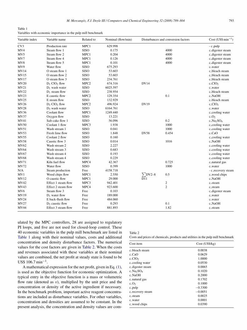
Table 1Variables with economic importance in the pulp mill benchmark
Variable index Variable name Related to Nominal (flow/min) Disturbances and conversion factors Cost (US$ min−1)
CV3 Production rate MPC1 629.998 - c pulpMV4 Steam flow 1 SISO 0.175 4000 c digester steamMV5 Steam flow 2 MPC1 0.204 4000 c digester steamMV7 Steam flow 4 MPC1 0.126 4000 c digester steamMV8 Steam flow 5 MPC1 0.101 4000 c digester steamMV9 Water flow SISO 675.293 c waterMV14 O steam flow 1 SISO 53.603 c bleach steamMV15 O steam flow 2 SISO 53.603 c bleach steamMV17 O steam flow 3 SISO 234.761 c bleach steamMV20 D1 ClO2 flow MPC2 674.316 DV14 c ClO2
MV21 D1 wash water SISO 6025.597 c waterMV22 D1 steam flow SISO 238.954 c bleach steamMV23 E caustic flow MPC2 129.354 0.1 c NaOHMV25 E steam flow SISO 132.929 c bleach steamMV26 D2 ClO2 flow MPC2 496.924 DV19 c ClO2
MV28 D2 wash water SISO 6164.761 c waterMV36 Coolant flow MPC1 1249.440 c cooling waterMV37 Oxygen flow SISO 13.221 c O2
MV41 Salt-cake flow 1 SISO 56.096 0.2 c Na2SO4
MV50 Coolant 1 flow MPC3 1.938 1000 c cooling waterMV51 Wash stream 1 SISO 0.041 1000 c cooling waterMV53 Fresh lime flow SISO 1.848 DV58 0.454 c CaOMV55 Coolant 2 flow SISO 0.160 c cooling waterMV58 Caustic flow 3 SISO 0.014 1016 c NaOHMV62 Wash stream 2 SISO 2.227 c cooling waterMV64 Wash stream 3 SISO 0.683 c cooling waterMV67 Wash stream 4 SISO 0.193 c cooling waterMV68 Wash stream 4 SISO 0.229 c cooling waterMV71 Kiln fuel flow MPC4 42.367 0.725 c natural gasMV72 Water flow SISO 0.399 1000 c waterN/A Steam production Free 4158.718 - c recovery steamMV1 Wood chips flow MPC1 2.550
∑DV2–8 0.5 c wood chips
MV12 O caustic flow MPC1 29.000 D11 c NaOHMV42 Effect 1 steam flow MPC3 942.401 2 c steamMV43 Effect 2 steam flow MPC4 923.600 2 c steamMV6 Steam flow 3 Free 0.103 c digester steamMV19 D1 water flow Free 189.000 c waterMV24 E back-flush flow Free 484.060 c waterM 0.1 c NaOHM 1.82 c steam
uP4TcvavU
itflcItcp
Table 2Costs and prices of chemicals, products and utilities in the pulp mill benchmark
Cost item Cost (US$/kg)
c bleach steam 0.0038c CaO 0.0629c ClO2 1.0000c cooling water 0.0530c digester steam 0.0065c Na2SO4 0.1020c NaOH 0.2000c natural gas 0.1702c O2 0.1000c pulp −0.3300
V27 D2 caustic flow Free 0.293V44 Effect 3 steam flow Free 881.893
lated by the MPC controllers, 28 are assigned to regulatoryI loops, and five are not used for closed-loop control. These0 economic variables in the pulp mill benchmark are listed inable 1 along with their nominal values, costs and additionaloncentration and density disturbance factors. The numericalalues for the cost factors are given in Table 2. When the costsnd revenues associated with these variables at their nominalalues are combined, the net profit at steady state is found to beS$ 106.7 min−1.A mathematical expression for the net profit, given in Eq. (1),
s used as the objective function for economic optimization. Aypical entry in the objective function is a mass or volumetricow rate (denoted as v), multiplied by the unit price and theoncentration or density of the active ingredient if necessary.
n the benchmark problem, important active reagent concentra-ions are included as disturbance variables. For other variables,oncentration and densities are assumed to be constant. In theresent analysis, the concentration and density values are com-c recovery steam −0.0051c steam 0.0025c water 0.0001c wood chips 0.0390
7 and C
brbcfp
f
3d
oespascairovb
pauadtvvt
3
tbtmbo
dfvtt
gmfew2aba
K
oe
b
−−
1 −
bvvto
3
tmooe
94 M. Mercangoz, F.J. Doyle III / Computers
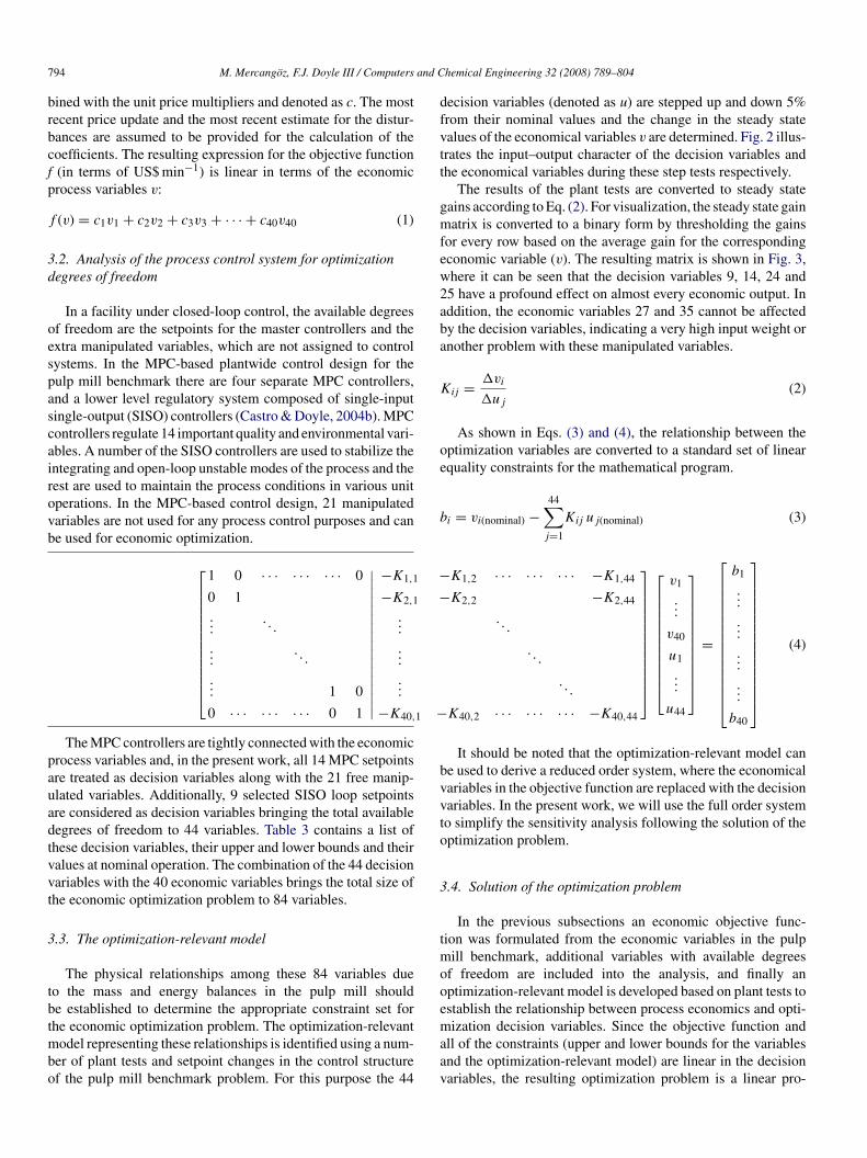
ined with the unit price multipliers and denoted as c. The mostecent price update and the most recent estimate for the distur-ances are assumed to be provided for the calculation of theoefficients. The resulting expression for the objective function(in terms of US$ min−1) is linear in terms of the economicrocess variables v:
(v) = c1v1 + c2v2 + c3v3 + · · · + c40v40 (1)
.2. Analysis of the process control system for optimizationegrees of freedom
In a facility under closed-loop control, the available degreesf freedom are the setpoints for the master controllers and thextra manipulated variables, which are not assigned to controlystems. In the MPC-based plantwide control design for theulp mill benchmark there are four separate MPC controllers,nd a lower level regulatory system composed of single-inputingle-output (SISO) controllers (Castro & Doyle, 2004b). MPControllers regulate 14 important quality and environmental vari-bles. A number of the SISO controllers are used to stabilize thentegrating and open-loop unstable modes of the process and theest are used to maintain the process conditions in various unitperations. In the MPC-based control design, 21 manipulatedariables are not used for any process control purposes and cane used for economic optimization.
The MPC controllers are tightly connected with the economicrocess variables and, in the present work, all 14 MPC setpointsre treated as decision variables along with the 21 free manip-lated variables. Additionally, 9 selected SISO loop setpointsre considered as decision variables bringing the total availableegrees of freedom to 44 variables. Table 3 contains a list ofhese decision variables, their upper and lower bounds and theiralues at nominal operation. The combination of the 44 decisionariables with the 40 economic variables brings the total size ofhe economic optimization problem to 84 variables.
.3. The optimization-relevant model
The physical relationships among these 84 variables dueo the mass and energy balances in the pulp mill shoulde established to determine the appropriate constraint set for
⎡⎢⎢⎢⎢⎢⎢⎢⎢⎢⎢⎢⎣
1 0 · · · · · · · · · 0
0 1...
. . .
.... . .
... 1 0
0 · · · · · · · · · 0 1
∣∣∣∣∣∣∣∣∣∣∣∣∣∣∣∣∣
−K1,1
−K2,1
...
...
...
−K40,
he economic optimization problem. The optimization-relevantodel representing these relationships is identified using a num-
er of plant tests and setpoint changes in the control structuref the pulp mill benchmark problem. For this purpose the 44
maav
hemical Engineering 32 (2008) 789–804
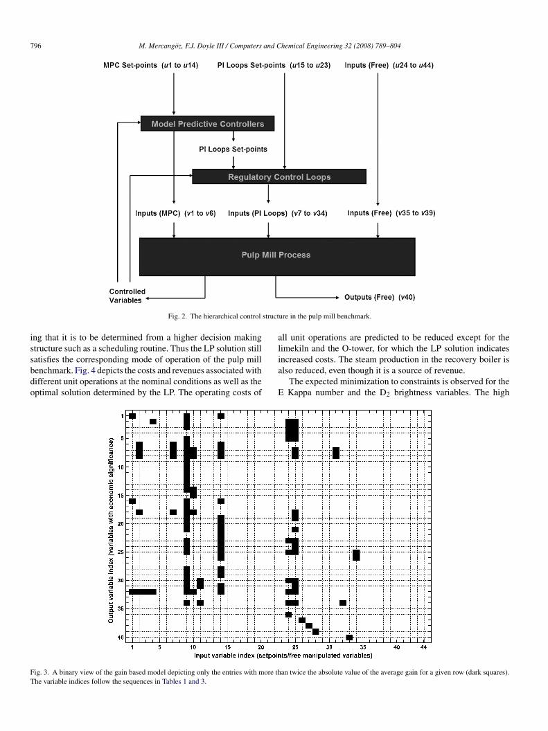
ecision variables (denoted as u) are stepped up and down 5%rom their nominal values and the change in the steady statealues of the economical variables v are determined. Fig. 2 illus-rates the input–output character of the decision variables andhe economical variables during these step tests respectively.
The results of the plant tests are converted to steady stateains according to Eq. (2). For visualization, the steady state gainatrix is converted to a binary form by thresholding the gains
or every row based on the average gain for the correspondingconomic variable (v). The resulting matrix is shown in Fig. 3,here it can be seen that the decision variables 9, 14, 24 and5 have a profound effect on almost every economic output. Inddition, the economic variables 27 and 35 cannot be affectedy the decision variables, indicating a very high input weight ornother problem with these manipulated variables.
ij = �vi
�uj
(2)
As shown in Eqs. (3) and (4), the relationship between theptimization variables are converted to a standard set of linearquality constraints for the mathematical program.
i = vi(nominal) −44∑
j=1
Kij uj(nominal) (3)
K1,2 · · · · · · · · · −K1,44
K2,2 −K2,44
. . .
. . .
. . .
K40,2 · · · · · · · · · −K40,44
⎤⎥⎥⎥⎥⎥⎥⎥⎥⎥⎥⎥⎦
⎡⎢⎢⎢⎢⎢⎢⎢⎢⎢⎢⎣
v1
...
v40
u1
...
u44
⎤⎥⎥⎥⎥⎥⎥⎥⎥⎥⎥⎦
=
⎡⎢⎢⎢⎢⎢⎢⎢⎢⎢⎢⎢⎢⎢⎣
b1
...
...
...
...
b40
⎤⎥⎥⎥⎥⎥⎥⎥⎥⎥⎥⎥⎥⎥⎦
(4)
It should be noted that the optimization-relevant model cane used to derive a reduced order system, where the economicalariables in the objective function are replaced with the decisionariables. In the present work, we will use the full order systemo simplify the sensitivity analysis following the solution of theptimization problem.
.4. Solution of the optimization problem
In the previous subsections an economic objective func-ion was formulated from the economic variables in the pulp
ill benchmark, additional variables with available degreesf freedom are included into the analysis, and finally anptimization-relevant model is developed based on plant tests tostablish the relationship between process economics and opti-
ization decision variables. Since the objective function andll of the constraints (upper and lower bounds for the variablesnd the optimization-relevant model) are linear in the decisionariables, the resulting optimization problem is a linear pro-

M. Mercangoz, F.J. Doyle III / Computers and Chemical Engineering 32 (2008) 789–804 795
Table 3Decision variables used by the economic optimization methodology
Variable index Variable name Related to Lower bound Nominal value Upper bound
CV3 D2 production rate MPC1 629.979 629.998 630CV4 Digester Kappa MPC1 12.5 19.9993 27.5CV8 Digester upper EA MPC1 2.39994233 9.59977 16.79959631CV9 Digester lower EA MPC1 2.250018703 9.00007 15.75013092CV10 Upper extract conductivity MPC1 17.46057706 69.8423 122.2240394CV11 Lower extract conductivity MPC1 12.11756028 48.4702 84.82292196CV19 O kappa MPC1 5 9.99972 15CV22 E kappa MPC2 2.4 2.5 2.6CV24 E washer [OH] MPC2 0.000449992 0.00085 0.001249992CV26 D2 brightness MPC2 0.8 0.81 0.84CV44 Black liquor solids MPC3 0.625 0.65001 0.675CV62 Slaker temperature MPC3 669.0120255 674.012 679.0120255CV79 Kiln O2 excess % MPC4 0.014965398 0.03497 0.054965398CV81 Kiln CaCO3 residual % MPC4 0.024871656 0.02487 0.024871656CV15 Digester liquor temperature SISO 425.5 435.5 445.5CV20 O tower temperature SISO 368 371 373.55CV21 D1 tower temperature SISO 329 339 347.4999999CV23 E0 tower temperature SISO 344 349 353.2499999CV25 D2 tower temperature SISO 343 348 352.2499999CV36 O tower consistency SISO 0.05 0.1 0.1425CV113 Recaust CaOH2 concentration SISO 3 18 30.75CV82 WL temperature SISO 358 368 376.4999999CV84 WL NaOH concentration SISO 99.14983595 100 150u6 Steam flow 3 (digester) Free 0.0373375 0.103 0.18025u13 Excess WL split (digester) Free 0.9 1 1.1u19 D1 water flow Free 68.51250002 189 330.75u24 E back-flush flow Free 240 484.06 847.105u27 D2 caustic flow Free 0.07325 0.293 0.4797875u32 Split fraction 6 (brown stock) Free 0.293617021 0.31915 0.340851064u34 Split fraction 8 (brown stock) Free 0.7176 0.78 0.83304u35 Split fraction 9 (brown stock) Free 0.38 0.4 0.417u39 Split fraction 1 (MEE) Free 0.720203732 0.9 1.575u44 Effect 3 steam flow (MEE) Free 821.9245866 881.893 952.4448u61 Filter lower flow (filter 2) Free 0.54 0.862 1.5085u69 Kiln primary air flow Free 62.5 250 437.5u73 Effect 5 exit flow (MEE) Free 75 300 525u74 Effect 4 exit flow (MEE) Free 75 300 525u75 Effect 3 exit flow (MEE) Free 75 300 525u76 Effect 6 exit flow (MEE) Free 75 300 525u77 Effect 2 exit flow (MEE) Free 75 300 525u78 Effect 1a exit flow (MEE) Free 75 300 525u79 Effect 1b exit flow (MEE) Free 75 300 525uu
g
aTcc
ltpsplrv
wm
80 Effect 1c exit flow (MEE) Free82 Coolant 4 flow (post Slaker) Free
ramming (LP) problem as shown in Eq. (5).
minu
cTv
s.t.
[ I| −K ]
[v
u
]= b
ulow < u < uhigh
vlow < v < vhigh
(5)
The solution to the problem in Eq. (5) is obtained easily using
n LP solver (MATLAB Optimization Toolbox linprog routine).he location of the optimal solution for LP problems lies on theonstraints. In the solution of this problem, seven variables areonstrained by upper bounds, 15 variables are constrained byiaaa
75 300 5252.5 10 17.5
ower bounds, and the remaining 62 variables are constrained byhe 40 equality constraints representing the plant model. Shadowrices in an LP are a measure of the sensitivity of the optimalolution to the location of the constraints. The important shadowrices in the solution of the economic optimization problem areisted in Table 4. It should be noted that each equality constraintepresenting the plant model is associated with one economicariable, but can constrain multiple decision variables.
The LP solution predicts a new set of operating conditions,hich can increase the net profit rate in the pulp mill bench-ark from US$ 106.7 to 126.4 min−1, corresponding to an 18%
ncrease. At this point it should be clarified that the constraintsround the E Kappa number and D2 brightness are kept within4% and 1.2% range, respectively, from their nominal values,
nd the production rate is not allowed to vary at all, consider-
796 M. Mercangoz, F.J. Doyle III / Computers and Chemical Engineering 32 (2008) 789–804
struct
issbdo
al
FT
Fig. 2. The hierarchical control
ng that it is to be determined from a higher decision makingtructure such as a scheduling routine. Thus the LP solution still
atisfies the corresponding mode of operation of the pulp millenchmark. Fig. 4 depicts the costs and revenues associated withifferent unit operations at the nominal conditions as well as theptimal solution determined by the LP. The operating costs ofia
E
ig. 3. A binary view of the gain based model depicting only the entries with more thhe variable indices follow the sequences in Tables 1 and 3.
ure in the pulp mill benchmark.
ll unit operations are predicted to be reduced except for theimekiln and the O-tower, for which the LP solution indicates
ncreased costs. The steam production in the recovery boiler islso reduced, even though it is a source of revenue.The expected minimization to constraints is observed for theKappa number and the D2 brightness variables. The high
an twice the absolute value of the average gain for a given row (dark squares).

M. Mercangoz, F.J. Doyle III / Computers and C
Table 4Shadow prices of selected constraints from the LP solution
Variable index Variable name Shadow price
Upper boundsCV36 O tower consistency 0.257CV3 D2 production rate 0.191CV8 Digester upper EA 0.132MV32 Split fraction 6 (brown stock) 0.085MV27 D2 caustic flow 0.067MV35 Split fraction 9 (brown stock) 0.066MV34 Split fraction 8 (brown stock) 0.033
Lower boundsCV24 E washer [OH] 3051.417CV81 Kiln CaCO3 residual % 602.592MV58 Caustic flow 3 (post WLC) 162.687CV26 D2 brightness 57.407MV8 Steam flow 5 (digester) 30.522MV39 Split fraction 1 (MEE) 17.376MV7 Steam flow 4 (digester) 16.880CV79 Kiln O2 excess % 12.582MV6 Steam flow 3 (digester) 3.011CV22 E Kappa 0.620MV61 Filter lower flow (filter 2) 0.251CV15 Digester liquor temperature 0.041CV84 WL NaOH concentration 0.025MV41 Salt-cake flow 1 (MEE) 0.018MV20 D1 ClO2 flow 0.011
Equality constraintsMV58 Caustic flow 3 (post WLC) 40.512MV6 Steam flow 3 (digester) 26.080MV4 Steam flow 1 (digester) 26.080MV5 Steam flow 2 (digester) 26.080MV1 Wood chips flow 22.683MV7 Steam flow 4 (digester) 9.199MV53 Fresh lime flow (causticizers) 1.001MV72 Mill water flow (MEE) 0.132MV71 Kiln fuel flow 0.123MV37 Oxygen flow (O reactor) 0.102CV3 D2 production rate −0.138MV8 Steam flow 5 (digester) −4.442
stultA
4
ftmdp
•
•
•
•
4s
de
Fig. 4. Comparison of the costs and revenues in the pulp mill bench
hemical Engineering 32 (2008) 789–804 797
hadow price for the production rate upper bound also suggestshat if it were allowed to vary, it would have been moved to itspper bound. However, the LP solution does not set the blackiquor solids content to its maximum value. The delignificationargets are reduced for the digester and increased for the O-tower.
uniform trend for operating temperatures is not observed.
. On-line optimization of the pulp mill benchmark
In the previous section, an economic optimization problem isormulated and solved for the pulp mill benchmark by treatinghe benchmark simulator as the data generator for an actual pulp
ill. This optimization problem can provide a foundation for theesign of a two-tier RTO system for the pulp mill benchmarkroblem. In this section the following tasks will be performed:
An optimizer will be developed and interfaced with the pro-cess control structure in the pulp mill benchmark. Initiallythe optimizer will transition the benchmark from the nominaloperating conditions to the solution determined by the LP.At the new operating region, a bias update will be carried out toimprove the accuracy of the optimization-relevant model. TheRTO system will readjust the plant according to the improvedpredictions.After the bias update, a sensitivity analysis on the RTO sys-tem will be evaluated to determine the cases where an RTOapplication will be beneficial.According to the sensitivity analysis the RTO system will betested in four scenarios for the effects of process disturbancesand changes in reagent and utility prices.
.1. Transition from nominal operation towards the LPolution
The closed-loop RTO design considered in this section isepicted in Fig. 5. The optimizer receives external market param-ters and disturbance estimates at each execution step to update
mark at nominal operation and according to the LP solution.

798 M. Mercangoz, F.J. Doyle III / Computers and Chemical Engineering 32 (2008) 789–804
d cont
tTtso
oift1w
at0Tip
u
Fa
Fig. 5. The three layer hierarchical arrangement of optimization an
he cost factors in the objective function in an on-line manner.he LP solution is updated, based on the new parameters, and
he updated solution is applied to the process by changing theetpoints for the MPC and SISO controllers as well as the valuesf the free manipulated variables.
The proposed RTO system is added to the SIMULINK filef the pulp mill benchmark along with a profit soft-sensor andt is interfaced with the existing control system. The execution
requency of the optimizer for the substantial transition fromhe nominal operation towards the LP solution is chosen to be00 min. To ensure a smooth transition, the operation is startedith the nominal setpoints and manipulated variable values unomiit
ig. 6. Comparison of the costs and revenues in the pulp mill benchmark at nominalfter the implementation of the LP solution on the benchmark.
rol tasks in the pulp mill benchmark after the addition of the RTO.
nd a “forgetting factor” h is used to ramp the nominal settingsowards the LP solution uLP by increasing h from 0 to 1 by.1 increments at every RTO execution as shown in Eq. (6).he costs and revenues at the resulting steady state operation
s shown in Fig. 6 and the dynamic transition data for selectedulp mill benchmark variables is presented in Fig. 7.
= huLP − (h − 1)unom (6)
The results show that the net profit rate in the benchmark isncreased from 106.7 to US$ 118.8 min−1 indicating a 12.3%mprovement which is short of the 18% increase predicted byhe LP solution. However, this number translates into more than
operation, according to the LP solution and according to the simulation results

M. Mercangoz, F.J. Doyle III / Computers and Chemical Engineering 32 (2008) 789–804 799
nomin
1wsdcTRot
csthptbcantaoa
4
et
fab
B
b
gtLrstsbpo
4
ss
Fig. 7. Dynamic transition data for selected variables from the
7% reduction of operating costs in the pulp mill benchmark,hich is still significant. Analysis of results for individual units
how that the optimizer is most efficient for the operation of theigester, D1-tower and the recausticizing areas and least effi-ient for the reduction of costs in the multi-effect evaporators.he large offsets between the targets generated by the LP basedTO and the actual steady state results indicate that the accuracyf the optimization-relevant model has deteriorated during theransition.
The violation of constraints on the variables at steady statean be an important concern. In this optimization algorithm, theetpoints are the decision variables and the resulting outputs arehe manipulated variable levels. Since the manipulated variablesave hard bounds, which cannot be violated, the only violationossible is in the controlled variables. The setpoints for the con-rolled variables are determined to respect their upper and lowerounds, but if the control structure cannot provide offset freeontrol, some controlled variables will violate their constraintst the new steady state. Digester Kappa number, O-tower Kappaumber, and the D2-tower brightness shown in Fig. 7 are con-rolled variables. The O-tower Kappa number is observed to haven offset, but its value is within acceptable bounds. There arether controlled variables with some steady state offset, whichre not shown in Fig. 7, but a constraint violation is not observed.
.2. Bias updating
A common method of improving the accuracy of simple mod-ls is the use of a bias term to make up for the difference betweenhe observed and predicted values (Ljung, 1998). Such bias terms
titm
al operating region to the LP solution under RTO supervision.
or the optimization-relevant model of this study can be defineds in Eq. (7) and the right hand side of the model equations cane updated as shown in Eq. (8).
i = vi,real − vi,predicted (7)
i = vi(nominal) −44∑
j=1
Kij uj(nominal) + Bi (8)
The pulp mill benchmark operating at the steady state tar-ets provided by the LP solution is used to calculate the biaserms. In the next step, the targets are updated by re-solving theP problem according to the optimization-relevant model, cor-
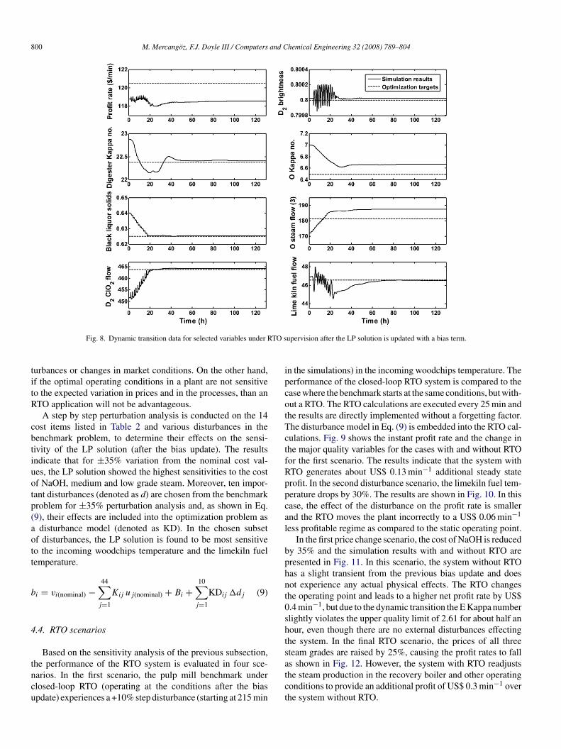
ected with the bias values. The RTO system is operated with theame settings given in the previous subsection. The dynamicalransition results after the bias update is provided in Fig. 8. Aignificant change is not observed in the net profit rate after theias correction. However, the sum of the absolute error in therediction of the 40 economical variables is reduced by an orderf magnitude, from a value of 1190.6–132.7.
.3. Sensitivity analysis for real-time optimization
Although the RTO system detailed in the previous sub-ections is used solely to steer the benchmark problem in aupervised fashion, the real purpose of RTO is to make proac-
ive changes to the operating policies in an autonomous fashionn the face of process disturbances and changing market condi-ions. The benefit from real-time optimization is expected to beore significant if the process economics are sensitive to dis-
800 M. Mercangoz, F.J. Doyle III / Computers and Chemical Engineering 32 (2008) 789–804
TO s
titR
cbtiuotp(aott
b
4
tncu
ipcotTctfRppcal
bphnt0shts
Fig. 8. Dynamic transition data for selected variables under R
urbances or changes in market conditions. On the other hand,f the optimal operating conditions in a plant are not sensitiveo the expected variation in prices and in the processes, than anTO application will not be advantageous.
A step by step perturbation analysis is conducted on the 14ost items listed in Table 2 and various disturbances in theenchmark problem, to determine their effects on the sensi-ivity of the LP solution (after the bias update). The resultsndicate that for ±35% variation from the nominal cost val-es, the LP solution showed the highest sensitivities to the costf NaOH, medium and low grade steam. Moreover, ten impor-ant disturbances (denoted as d) are chosen from the benchmarkroblem for ±35% perturbation analysis and, as shown in Eq.9), their effects are included into the optimization problem as
disturbance model (denoted as KD). In the chosen subsetf disturbances, the LP solution is found to be most sensitiveo the incoming woodchips temperature and the limekiln fuelemperature.
i = vi(nominal) −44∑
j=1
Kij uj(nominal) + Bi +10∑
j=1
KDij �dj (9)
.4. RTO scenarios
Based on the sensitivity analysis of the previous subsection,
he performance of the RTO system is evaluated in four sce-arios. In the first scenario, the pulp mill benchmark underlosed-loop RTO (operating at the conditions after the biaspdate) experiences a +10% step disturbance (starting at 215 minatct
upervision after the LP solution is updated with a bias term.
n the simulations) in the incoming woodchips temperature. Theerformance of the closed-loop RTO system is compared to thease where the benchmark starts at the same conditions, but with-ut a RTO. The RTO calculations are executed every 25 min andhe results are directly implemented without a forgetting factor.he disturbance model in Eq. (9) is embedded into the RTO cal-ulations. Fig. 9 shows the instant profit rate and the change inhe major quality variables for the cases with and without RTOor the first scenario. The results indicate that the system withTO generates about US$ 0.13 min−1 additional steady staterofit. In the second disturbance scenario, the limekiln fuel tem-erature drops by 30%. The results are shown in Fig. 10. In thisase, the effect of the disturbance on the profit rate is smallernd the RTO moves the plant incorrectly to a US$ 0.06 min−1
ess profitable regime as compared to the static operating point.In the first price change scenario, the cost of NaOH is reduced
y 35% and the simulation results with and without RTO areresented in Fig. 11. In this scenario, the system without RTOas a slight transient from the previous bias update and doesot experience any actual physical effects. The RTO changeshe operating point and leads to a higher net profit rate by US$.4 min−1, but due to the dynamic transition the E Kappa numberlightly violates the upper quality limit of 2.61 for about half anour, even though there are no external disturbances effectinghe system. In the final RTO scenario, the prices of all threeteam grades are raised by 25%, causing the profit rates to fall
s shown in Fig. 12. However, the system with RTO readjustshe steam production in the recovery boiler and other operatingonditions to provide an additional profit of US$ 0.3 min−1 overhe system without RTO.
M. Mercangoz, F.J. Doyle III / Computers and Chemical Engineering 32 (2008) 789–804 801
Fig. 9. Dynamic response of the pulp mill benchmark to a +10% step disturbance in incoming wood chips temperature for scenarios with and without RTO.
ease i
5
pttt
ems
Fig. 10. Dynamic response of the pulp mill benchmark to a 30% decr
. Discussion of results
In this paper, an RTO system for the pulp mill benchmark
roblem is formulated. For this purpose, an economic optimiza-ion problem is developed by taking the process economics andhe available degrees of freedom in the benchmark control struc-ure into account. A linear steady state model is developed totaic
n the limekiln fuel temperature for scenarios with and without RTO.
stablish the relationships among the variables chosen for opti-ization and the resulting linear set of equations are used in the
olution of the LP problem as equality constraints. Solution of
he LP is implemented on the pulp mill benchmark by interfacingn RTO unit with the existing control system. The RTO systems later tested in four scenarios, where process disturbances andhanges in reagent and utility prices are considered.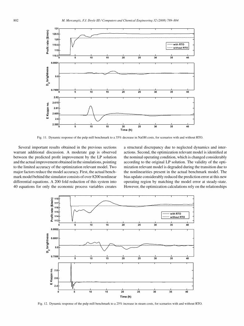
802 M. Mercangoz, F.J. Doyle III / Computers and Chemical Engineering 32 (2008) 789–804
5% d
wbatmmd4
aatam
Fig. 11. Dynamic response of the pulp mill benchmark to a 3
Several important results obtained in the previous sectionsarrant additional discussion. A moderate gap is observedetween the predicted profit improvement by the LP solutionnd the actual improvement obtained in the simulations, pointingo the limited accuracy of the optimization relevant model. Two
ajor factors reduce the model accuracy. First, the actual bench-ark model behind the simulator consists of over 8200 nonlinear
ifferential equations. A 200 fold reduction of this system into0 equations for only the economic process variables creates
tboH
Fig. 12. Dynamic response of the pulp mill benchmark to a 25% i
ecrease in NaOH costs, for scenarios with and without RTO.
structural discrepancy due to neglected dynamics and inter-ctions. Second, the optimization relevant model is identified athe nominal operating condition, which is changed considerablyccording to the original LP solution. The validity of the opti-ization relevant model is degraded during the transition due to
he nonlinearities present in the actual benchmark model. Theias update considerably reduced the prediction error at this newperating region by matching the model error at steady-state.owever, the optimization calculations rely on the relationships
ncrease in steam costs, for scenarios with and without RTO.
and C
owbiRanf(
bfusoitebdalp
cteaiasCtRea21asf
noadrsvvbba2ntp
topttattncAcnp
6
tapsmtotc
A
otMCa
R
B
B
B
C
C
C
M. Mercangoz, F.J. Doyle III / Computers
f the different decision variables with respect to each other,hich are represented by the gains Kij in the model. After theias update, the second RTO scenario results in reduced prof-tability that is caused by inaccurate predictions of the model.ather than a bias update, these gains can be updated for anctual improvement of the optimization relevant model at theew operating region. Methods for designing plant experimentsor model based RTO can be found in reference Yip and Marlin2003).
The use of plantwide identification experiments should alsoe discussed from an industrial point of view. The time scalesor pulp mills are quite long and process disturbances and sched-led operational changes can reduce the accuracy of plantwidetep tests or make them completely impractical. However, theptimization methodology presented in this paper is not lim-ted by such a procedure. The only requirement is to obtainhe gains between the optimization decision variables and theconomic variables. In an industrial setting, such models cane conveniently developed by combining historical closed loopata, simple steady state simulators, and limited plant tests. Theccuracy of the optimization relevant model in this study is quiteimited and still a 17% reduction of operating costs is madeossible.
The sensitivity analysis after the bias update revealed fourases where on-line optimization could be beneficial comparedo keeping the process at a static operating point. The differ-nces between RTO based and static strategies for these casesre demonstrated in simulation scenarios. In three cases, the RTOmproved the profitability by an average of US$ 0.27 min−1 orbout US$ 130,000 per year. In one case, the RTO resulted inlightly less profitable operation due to the errors in the model.onsidering that four parameters out of 14 prices and 10 dis-
urbances ended up shifting the location of the LP solution, anTO application can be beneficial for more than 15% of thexpected changes. This observation can put the value of an RTOpplication to 15% of US$ 130,000, which will be about US$0,000 per year. However, it should be noted that the original7% reduction in operating costs corresponds to US$ 6 millionnnual savings, which is enabled by the same economic analy-is, model development and optimization tools that were usedor the RTO.
The dynamic response of the pulp mill benchmark to eco-omic optimization should be discussed as well. In the originalptimization, and also after the bias update, the plant takesbout 80 h to settle to the new operating region. This valueepends on the size of the forgetting factor or the rampate, but a faster transition results in violation of quality con-traints and even instability of certain units. Some controlledariables such as the D2 brightness and some manipulatedariables such as the limekiln fuel flow experience oscillatoryehavior even at the current transition rate. This observationrings about another connection between the control systemnd economic optimization beyond the discussion in Section
. The original control system for the benchmark problem isot designed to perform together with an on-line optimiza-ion system and the tuning can be revised for better trackingerformance.C
hemical Engineering 32 (2008) 789–804 803
As far as the dynamics are concerned, the RTO based sys-em generally goes through a relatively less profitable transientf 5–10 h due to the utility costs of re-adjusting the operatingoint and the plant settles in less than 40 h. The economics of theransient response is not addressed in this paper and a combina-ion of RTO and MPC studies (Zanin et al., 2002; Engell, 2006)nd a grade change approach are necessary for the solution ofhat problem. Clearly, the process is operating much closer tohe minimum pulp quality requirements after the original eco-omic optimization and it is quite possible to have more frequentonstraint violations during dynamic transients under an RTO.lso, the effect of RTO execution frequency and other RTO
omponents such as steady state detection or the profit sensor isot considered in this paper, but they are very important for theerformance of an RTO system.
. Conclusion
In this work, an economic optimization methodology forhe pulp mill benchmark problem is presented. A plantwidepproach to optimization is used and the relationship betweenlantwide process control and economic optimization is demon-trated in the development of an RTO for the pulp mill bench-ark. The application of the economic optimization results on
he benchmark simulator resulted in significant reduction ofperating costs. The proposed methodology in this paper treatedhe benchmark simulator as an actual mill and similar algorithmsan be applied to optimize the operation of existing pulp mills.
cknowledgement
The authors gratefully acknowledge the financial supportf the Process Systems Engineering Consortium (PSEC) ofhe University of California, Santa Barbara, University of
assachusetts Amherst, and University of Illinois at Urbanahampaign. The authors are grateful for the suggestions of thenonymous reviewers.
eferences
iegler, L. T., & Grossmann, I. E. (2004). Retrospective on optimization. Com-puters & Chemical Engineering, 28, 1169–1192.
rewster, D. B., Uronen, P., & Williams T. J. (1985). Hierarchical computer con-trol in the pulp and paper industry (Technical Report). West Lafayette, IN:Purdue Laboratory for Applied Industrial Control, School of Engineering,Purdue University.
lomberg, H., & Golemanov, L. A. (1973). Optimization of storage sizes andcontrol strategy in industrial production systems. Automatica, 9, 329–337.
astro, J. J., & Doyle, F. J. (2004a). A pulp mill benchmark problem for control:Problem description. Journal of Process Control, 14, 17–29.
astro, J. J., & Doyle, F. J. (2004b). A pulp mill benchmark problem for control:Application of plantwide control design. Journal of Process Control, 14,329–347.
heng, R., Forbes, J. F., & Yip, W. S. (2006). Coordinated decentralized MPC forplantwide control of a pulp mill benchmark problem. In Proceedings of the
IFAC Symposium on Advanced Control of Chemical Processes (ADCHEM)(pp. 35–40).ristina, H., Aguiar, I. L., & Filho, R. M. (1998). Modeling and optimizationof pulp and paper processes using neural networks. Computers & ChemicalEngineering, 22(Suppl.), S981–S984.

8 and C
C
D
D
D
DD
D
E
F
G
J
K
L
M
M
N
P
P
R
R
S
S
S
S
S
S
T
T
V
Y
04 M. Mercangoz, F.J. Doyle III / Computers
utler, C. R., & Perry, R. T. (1983). Real time optimization with multivariablecontrol is required to maximize profits. Computers & Chemical Engineering,7(5), 663–667.
abros, M., Perrier, M., Forbes, F., Fairbank, M., & Stuart, P. R. (2005). Model-based direct search optimization of the broke recirculation system in anewsprint mill. Journal of Cleaner Production, 13, 1416–1423.
eKing, N. (Ed.). (2004). Pulp and paper global fact & price book 2003–2004.Boston: Paperloop, Inc.
hak, J., Dahlquist, E., Holmstrom, K., Ruiz, J., Belle, J., & Goedsche, F. (2004).Developing a generic method for paper mill optimization. In Proceedings ofControl Systems Conference (pp. 207–214).
oE Annual Energy Review. (2004). Report No. DOE/EIA-0384.ogan, I., & Guruz, A. G. (2004). Waste minimization in a bleach plant.
Advances in Environmental Research, 8, 359–369.umont, G., Van Fleet, R., & Stewart, G. (2004). A setpoint generation tool for
optimal distribution of chemical loads betwen bleaching stages. In Proceed-ings of Control Systems Conference (pp. 95–97).
ngell, S. (2006). Feedback control for optimal process operation. In Proceed-ings of the IFAC Symposium on Advanced Control of Chemical Processes(ADCHEM) (pp. 13–26).
orbes, J. F., & Marlin, T. E. (1996). Design cost: A systematic approachto technology selection for model-based real-time optimization systems.Computers & Chemical Engineering, 20(6/7), 717–734.
eorgiou, A., Taylor, P., Galloway, R., Casey, L., & Sapre, A. (1997). Plantwideclosed loop real time optimization and advanced control of ethylene plant-(CLRTO) improves plant profitability and operability. In Proceedings ofNPRA Computer Conference.
aakko Poyry Management Consulting. (2003). World paper markets up to 2015:What drives the global demand? Tappi Solutions, 86(8), 64.
ayihan, F. (1997). Process systems management in the pulp and paper indus-tries: An optimization approach. Pulp & Paper Canada, 98(8), 37–40.
jung, L. (1998). System identification: Theory for the user (2nd ed.). UpperSaddle River, NJ: Prentice Hall.
ercangoz, M., & Doyle, F. J., III. (2006). Model-based control in the pulp andpaper industry. IEEE Control System Magazine, 26(4), 30–39.
orari, M., Stephanopoulos, G., & Arkun, Y. (1980). Studies in the synthesis
of control structures for chemical processes: Part I. AIChE Journal, 26(2),220–232.ilsson, K., & Soderstrom, M. (1992). Optimizing the operating strategy ofa pulp and paper mill using the MIND method. Energy, 17(10), 943–953.
Y
Z
hemical Engineering 32 (2008) 789–804
ettersson, J., Ledung, L., & Zhang, X. (2006). Decision support for pulpmill operations based on large-scale online optimization. In Proceedingsof Control Systems Conference (pp. 24–29).
rett, D., & Garcia, C. (1988). Fundamental process control. Stonelam, MA:Butterworth Publisher.
otava, O., & Zanin, A. C. (2005). Multivariable control and real-timeoptimization—An industrial practical view. Hydrocarbon Processing, 84(6),61–71.
unklera, T. A., Gerstorfer, E., Schlang, M., Junnemann, E., & Hollatz, J. (2003).Modeling and optimisation of a refining process for fibre board production.Control Engineering Practice, 11, 1229–1241.
antos, A., & Dourado, A. (1999). Global optimization of energy and productionin process industries: A genetic algorithm application. Control EngineeringPractice, 7, 549–554.
arimveis, H., Angelou, A., Retsina, T., & Bafas, G. (2003). Maximization ofprofit through optimal selection of inventory levels and production rates inpulp and paper mills. Tappi Journal, 2(7), 13–18.
eborg, D. E., Edgar, T. F., & Mellichamp, D. A. (2004). Process dynamics andcontrol (2nd ed.). Danvers, MA: John Wiley & Sons, Inc..
hih, C. S, & Krishnan, P. (1973). System optimization for pulp and paperindustrial wastewater treatment design. Water Research, 7(12), 1805–1820.
kogestad, S. (2000). Plantwide control: The search for the self-optimizingcontrol structure. Journal of Process Control, 10, 487–507.
mook, G. A. (1992). Handbook for pulp and paper technologists (2nd ed.).Vancouver, BC: Angus Wilde Publications.
hibault, J., Taylor, D., Yanofsky, C., Lanouette, R., Fonteix, C., & Zaras, K.(2003). Multicriteria optimization of a high yield pulping process with roughsets. Chemical Engineering Science, 58, 203–213.
osukhowong, T., Lee, J. M., Lee, J. H., & Lu, J. (2004). An introduction to adynamic plant-wide optimization strategy for an integrated plant. Computers& Chemical Engineering, 29, 199–208.
anbrugghe, C., Perrier, M., Desbiens, A., & Stuart, P. (2004). Real-time opti-mization of a bleach plant using an IMC-based optimization algorithm. InProceedings of Control Systems Conference (pp. 26–39).
ip, W. S., & Marlin, T. E. (2003). Designing plant experiments for real-timeoptimization systems. Control Engineering Practice, 11, 837–845.
oung, R. E. (2006). Petroleum refining process control and real-time optimiza-tion. IEEE Control System Magazine, 26(6), 73–83.
anin, A. C., Gouvea, M. T., & Odloak, D. (2002). Integrating Real-Time Opti-mization into the Model Predictive Controller of the FCC system. ControlEngineering Practice, 10(8), 819–831.