Real-time part sequencing in a flexible assembly cell: system development and evaluation

Engineering Costs and Production Economics, 2 1 ( 199 1) 11 l- 13 1 117 Elsevier

Real-time part sequencing in a flexible assembly cell: system development and evaluation

S.M.A. Suliman

College of Engineering, University of Bahrain, Bahrain

A.M. El-Tamimi

College ofEngineering, King Saud University, Saudi Arabia

and D.F. Williams

College of Manufacturing, Cranfield Institute of Technology, UK

(Received January 3, 1989; accepted in revised form November 29, 1990)

Abstract

This paper considers the development of a general part sequencing methodology which suits flexible systems. A flexible assembly cell configuration is conceptualized. The cell is characterized by a common buffer and a single flexible transfer device for inter-cell transfer activities. Since the time available for decision making on part sequencing is very short, a fast solution is required. A real-time computerized part sequencing system of modular structure is developed. The system comprises three functions: ENTER, ALLOCATE, and TRANSFER SEQUENCE. Each function is provided with various priority options to satisfy different company strategies. Computer simulation is used to compare alternative sequencing structures of the system developed, and to examine its effectiveness under different operating conditions with reference to cell performance and time response.

1. Introduction

Assembly systems are usually made up of work stations, peripheral and transfer devices for car- rying out assembly tasks. The flexible assembly cell (FAC ) concept is characterized by common transfer and control systems. The work stations of this cell are arranged in such a way that their pick-up and deposit areas are within the reach of the transfer device which has random access ca- pability (e.g., transfer robot or automatic guided vehicle). Another characteristic is the presence of a single central storage of limited capacity buffering storages for all work stations and also serving as a loading/unloading station. Such cells can be used for mid-volume, mixed-model assembly of small and medium-sized products, e.g., domestic electrical appliances, hydraulic com- ponents, and instruments.

The FAC has the same general features as a

flexible manufacturing system (FMS). Both are multi-stage production systems comprised of the same basic elements, specifically, work stations, transfer equipment, and control device. In each of these systems, parts move in a prescribed route through the different work stations where they are serviced. However, they have the following dis- tinct differences: First, the processing cycle time scale of an FMS is in the order of minutes while that of an FAC is in the order of a few seconds ( Wamecke and Walther [ 1 ] ). This implies that the time available for decision making on completion of an activity in an FAC is very short compared to that in an FMS.

Second, due to FAC short processing periods, the ratio of the transfer time to the processing time (transfer ratio) is very high when compared to that of the FMS. For such a high transfer ratio, transfer sequencing is expected to have an effect on cell performance when the transfer de-

0167-188X/91 /$03.50 0 1991-Elsevier Science Publishers B.V.

118

vice is the limiting factor. Third, in an FMS each individual part is an entity which may not be processed by more than one machine at a time, i.e. parts are sequentially processed. This condition is not true for assembly of individual parts where subassemblies can be processed simulta- neously at different work stations (parallel processing is allowed in FAC) until these subassemblies are brought together at some point to be assembled. This assembly environment adds two additional dimensions to the problem of part sequencing, since one must consider: l each subassembly as an entity for sequenc-

ing until it is completed, and become ready to merge with other subassemblies. l not only the subassemblies on hand at a given

work station, but also the dependent subassemblies that may be combined with these subassemblies at a later work station.

In a flexible assembly cell of mixed model production, the operation control problems which are concerned with sequencing of parts for assembly can be classified into: ( 1) Part-entry problem: which part type/model

to be entered into the cell. (2 ) Part-allocation problem: which part to be

allocated to an idle work station. ( 3 ) Trans~r-sequencing problem: which trans-

fer request to be serviced first. The part sequencing and scheduling proce-

dures for job shops and conventional assembly systems attempt to optimize certain criteria such as throughput and utilization (Ramesh and Cary [ 21). Such optimization is usually done off-line due to complexity of the techniques (Suliman et al. f 3 ] ) . The off-line solutions are difficult to ap- ply to a production system characterized by a changing environment due to processing time variability, machine breakdowns, power failure, and delay in supplies. The on-line control is an appropriate approach for such environment. This is an algorithmic solution method usually based on priority dispatching rules, and adopted for controlling of flexible manufactu~ng systems (Abdallah f 41, Blackstone et al. [ 5 1, Choi and Malstrom [ 6 1, Conway et al. [ 71, Gere [ 8 1, Panwalker and Iskander [ 91). The aim of this work is to develop a rational part sequencing methodology for a flexible assembly cell with ref-

erence to performance and decision lead time. An upper bound of one second is required for the time available to make a decision on the sequencing problem. This is because the processing time of an assembly operation is expected to be greater than one second and in the order of few seconds.

2. Part-sequencing system

The part-sequencing system consists of three main functions (ENTER, ALLOCATE, and TRANSFER SEQUENCE} and an auxiliary function (UPDATE). The main functions pro- vide decision making procedures for the sequencing problem, while the auxiliary function provides data management methods for data handling and updating.

This function is based on a ratio rule which tends to distribute evenly the different part types/ models over the production period. The rule can be stated as: Enter first the part type/model with the highest ratio of remaining production requirement waiting outside the cell (NPMJ ) to its original requirement at the beginning of production period (NPM,), i.e.,

where RAT, is the priority of part type/model j. Although this rule is activated by default, an al- lowance has been made to enable the user to in- troduce his own entry priority.

2.2 ALLOCATE function

The ALLOCATE function assigns a prime priority to each imminent operation. The operation having the highest prime priority is selected and the part requiring that operation is allocated to the corresponding work station. When an operation conflict occurs, the function provides two sets of rules one for work station conflict and the other for part conflict.

Due to the absence of a priority rule which per- forms good in all situations (Aanen et al. [ lo],

119

Suliman [ 1 1 ] ), it has been decided to build in the ALLOCATE function different priority rules. This enables the user to incorporate his company specifics in the sequencing system. Seventeen different options are provided for the prime priority and part conflict resolution. The options represent five priority groups covering a wide range of priorities used as sequencing and scheduling rules. The groups are: l processing time related rules l due-date related rules l number of operations related rules l arrival times related rules l others such as user specified priorities, least

allocation index and random selection. For work station conflict resolution, six options are available representing three priority groups, namely, work in progress, work load, and others such as first come first served and random selection.

An allocation index is brought to action by default as a primary priority. This index is defined as: If part P, requires work station W, for operation 01, then the allocation index k*j of operation 0, is given by the sum of the number of work stations competing for part i (NW,) and the number of parts competing for work station j (NP,), i.e.,

k,, = NW, + NP, (2)

The least allocation index rule (LAI) states that the part having operation with the smallest index is assigned to the work station required to per- form that operation.

2.3 TRANSFER SEQUENCE function

This function is based on an algorithm which includes an implicit ‘look-ahead’ heuristic aimed at reduced unloaded movements. The ‘look- ahead’ effect is manifested by avoiding the transfer device visiting of a work station twice (except the common buffer) while it is implementing a transfer sequence. For example, if an allocated work station j has a part on it which is allocated to another work station k, then work station j is serviced with its allocated part. Consequently, the part on work stationj is removed to work station k. Thus, a sequence of continuous loaded movements will be obtained.

Having generated all the possible loaded se- quences, they are prioritized using the shortest time rule for only the unloaded movements of the transfer robot. In other words, a priority is given to each loaded sequence according to the time required by the transfer device to move from its initial location to the first picking point of that loaded sequence. This algorithm is activated by default, however, it can be overridden by either the FCFS rule or a fixed transfer priority specified by the user.

2.4 UPDATE function

This is an auxiliary function for data handling and file updating. For efficient part-sequencing systems, the function is divided into seven subfunctions. Each subfunction is concerned with updating certain attributes of tiles which require simultaneous updating.

2.5 Part-sequencing procedure

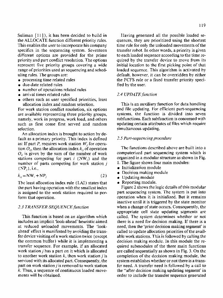
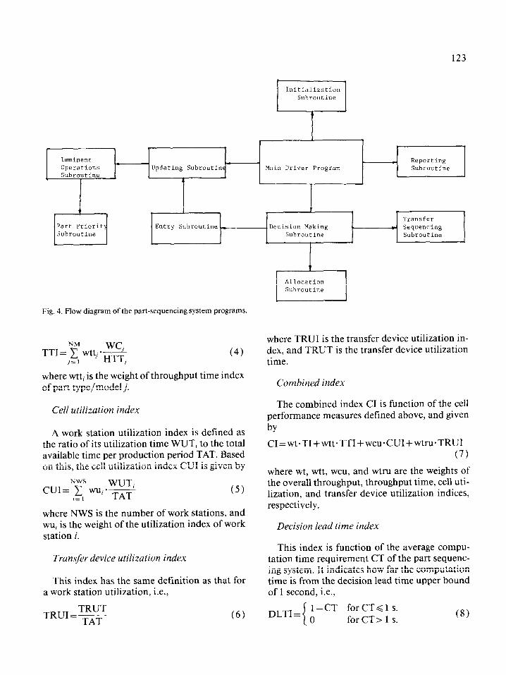
The functions described above are built into a computerized part sequencing system which is organized in a modular structure as shown in Fig. 1. The figure shows four main modules: l Initialization module l Decision making module l Updating module l Reporting module.

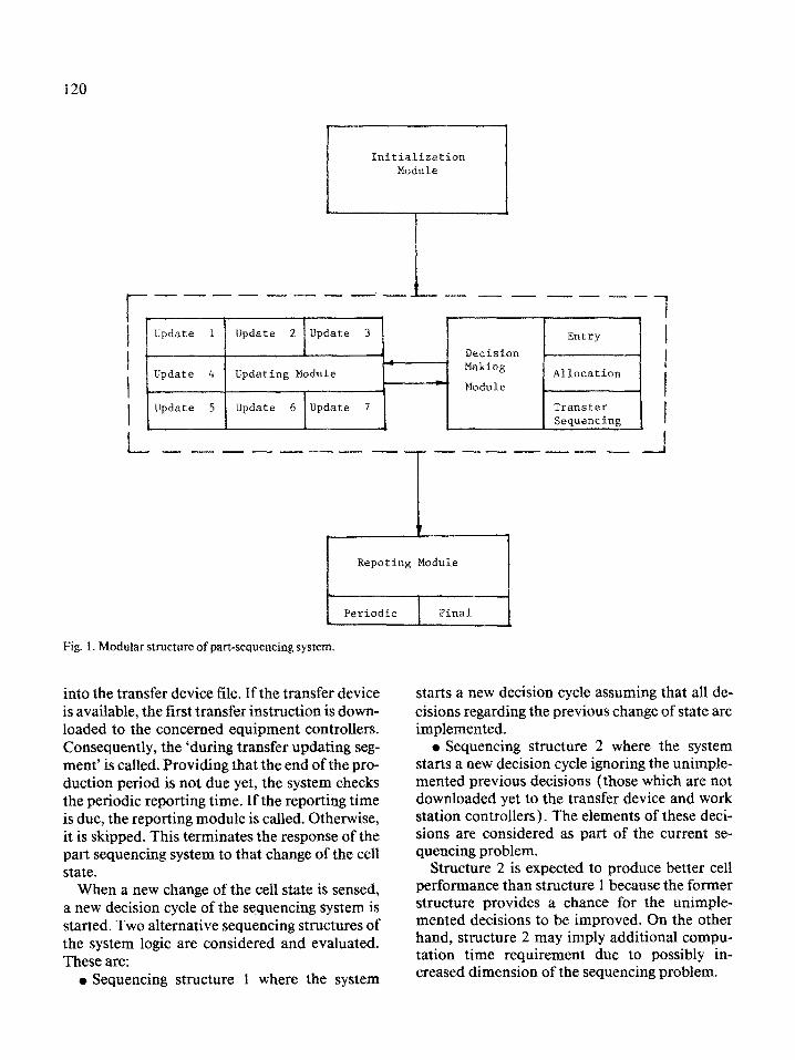
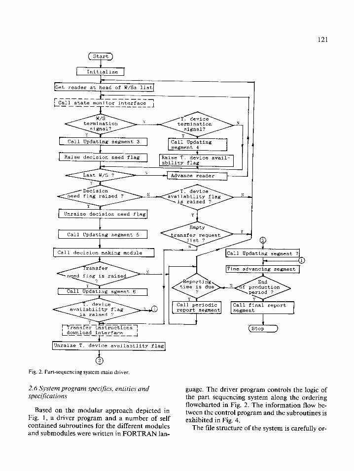
Figure 2 shows the logic details of this modular part sequencing system. The system is put into operation when it is initialized. But it remains inactive until it is triggered by the state monitor when a change of state occurs. Consequently, the appropriate cell state updating segments are called. The system determines whether or not there is a need for decision making. If there is a need, then the ‘prior decision making segment’ is called to update allocation priorities of the available work stations. This is followed by calling the decision making module. In this module the required submodules of the three main functions are called sequentially as shown in Fig. 3. On the completion of the decision making module, the system establishes whether or not there is a transfer need. A transfer need is followed by a call to the “after decision making updating segment’ in order to include the transfer sequence generated

120

Initialization

& Update 4 Updating Module

Kaking Allocation

--' Module

Update 5 Update 6 Update 7 Transfer Sequencing

Repoting Module

Fig. 1. Modular structure of part-sequencing system.

into the transfer device file. If the transfer device is available, the first transfer inst~~tio~ is downloaded to the concerned equipment controllers. Consequently, the ‘during transfer updating segment’ is called. Providing that the end of the production period is not due yet, the system checks the periodic reporting time. If the reporting time is due, the reporting module is called. Otherwise, it is skipped. This terminates the response of the part sequencing system to that change of the cell state.

When a new change of the cell state is sensed, a new decision cycle of the sequencing system is started. Two alternative sequencing structures of the system logic are considered and evaluated. These are:

o Sequencing st~~ture 1 where the system

starts a new decision cycle assuming that all decisions regarding the previous change of state are implemented.

o Sequencing structure 2 where the system starts a new decision cycle ignoring the unimplemented previous decisions (those which are not downloaded yet to the transfer device and work station controllers). The elements of these decisions are considered as part of the current sequencing problem.

Structure 2 is expected to produce better cell performance than structure I because the former structure provides a chance for the unimplemented decisions to be improved. On the other hand, structure 2 may imply additional computation time requirement due to possibly increased dimension of the sequencing problem.

121

r------ -------7 1 Call state monitor interface L-_-__ l----------

1

termination

Call Updating segment 3 Call Updating

1 Raise decision need flaa 1 rRaise T.

+ Call Updating segment 5

I t

Call decision making module

,T-

Call Updating sgment 6

Ldcnloadinterface T----J

2 4_ .ting

Time advancing segment

Call periodic Call final report report segment segment

stop

Unraise T. device availability flag

Fig. 2. Part-sequencingsystem main driver.

2.6 System program specifics, entities and specifications

Based on the modular approach depicted in

guage. The driver program controls the logic of the part sequencing system along the ordering flowcharted in Fig. 2. The information flow be-

Fig. 1, a driver program and a number of self contained subroutines for the different modules and submodules were written in FORTRAN lan-

tween the control program and the subroutines is exhibited in Fig. 4.

The file structure of the system is carefully or-

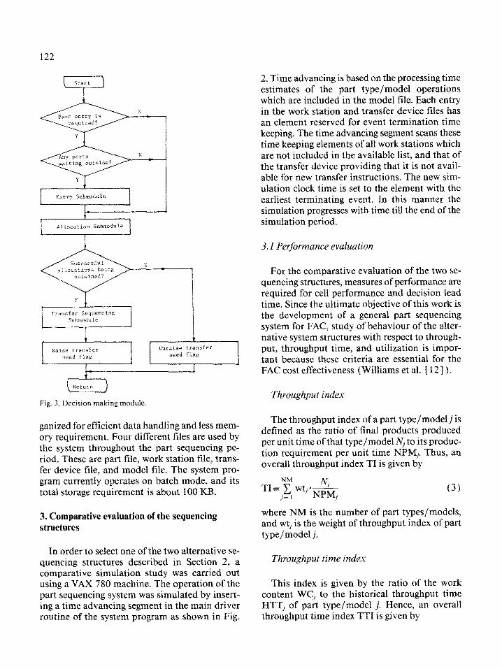
Fig. 3. Decision making module.

ganized for efficient data handling and less mem- ory requirement. Four different files are used by the system throu~out the part sequencing period. These are part file, work station file, transfer device Iile, and model file. The system program currently operates on batch mode, and its total storage requirement is about 100 KB.

3. Comparative evaluation of the sequencing structures

In order to select one of the two alternative sequencing structures described in Section 2, a comparative simulation study was carried out using a VAX 780 machine. The operation of the part sequencing system was simulated by insert- ing a time advancing segment in the main driver routine of the system program as shown in Fig.

2. Time advancing is based on the processing time estimates of the part type/model operations which are included in the model file. Each entry in the work station and transfer device files has an element reserved for event termination time keeping, The time advancing segment scans these time keeping elements of all work stations which are not included in the available list, and that of the transfer device providing that it is not available for new transfer instructions. The new simulation clock time is set to the element with the earliest terminating event. In this manner the simulation progresses with time till the end of the simulation period.

3.1 Performance evaluution

For the comparative evaluation of the two sequencing structures, measures of performance are required for cell performance and decision lead time. Since the ultimate objective of this work is the development of a general part sequencing system for FAC, study of behaviour of the alternative system structures with respect to throughput, throughput time, and utilization is impor- tant because these criteria are essential for the FAC cost effectiveness f Williams et al. [ 121).

The throughput index of a part typelmodelj is defined as the ratio of final products produced per unit time of that type/model Nj to its production requirement per unit time NPM,. Thus, an overall throughput index TI is given by

TIzNf w$-& j=l J

(3)

where NM is the number of part types/models, and wt, is the weight of throughput index of part type/model j,

~~ro~gh~~t time index

This index is given by the ratio of the work content WC, to the historical throughput time HTT,, of part type/model j. Hence, an overali throughput time index TTI is given by

123

Initialization Subroutine

.

, 1

Imminent Operations

- c Reporting Updating Subroutine Main Driver Program Subroutine

( Subroutine I

Part Priorit

t r I

I Transfer Entry Subroutine _ Decision Making Sequencing 1

, Subroutine

1

Subroutine

Fig. 4. Flow diagram of the part-sequencing system programs.

TTI=“cM wtti$$ /=I J

(4)

where wtt, is the weight of throughput time index of part type/modelj.

Cell utilization index

A work station utilization index is defined as the ratio of its utilization time WUT, to the total available time per production period TAT. Based on this, the cell utilization index CUI is given by

(5)

where NWS is the number of work stations, and wu, is the weight of the utilization index of work station i.

Transfer device utilization index

This index has the same definition as that for a work station utilization, i.e.,

where TRUI is the transfer device utilization index, and TRUT is the transfer device utilization time.

Combined index

The combined index CI is function of the cell performance measures defined above, and given

by

CI=wt~TI+wtt~TTI+wcu~CUI+wtru~TRUI (7)

where wt, wtt, wcu, and wtru are the weights of the overall throughput, throughput time, cell utilization, and transfer device utilization indices, respectively.

Decision lead time index

This index is function of the average computation time requirement CT of the part sequencing system. It indicates how far the computation time is from the decision lead time upper bound of 1 second, i.e.,

TRUI=s (6) (8)

124

Ideally a good part sequencing system can be considered when all the values of its indices approach unity.

3.2 Sirn~~ati#~ procedure

Different cell conditions were considered by varying cell size (NWS), number of part types/ models (NM), and cell traffic density (NPC). Three levels were selected for each of the first two conditioning factors (3, 5 and 7 for the cell size, and 3, 6 and 9 for the number of part types/ models), while two levels were selected for the traffic density (low and high).

Three different sets of sequencing rules were tested. These were obtained by taking three different options for the allocation primary rule, while the same entry and transfer sequencing rules, which are normally set by default, were used. The primary rules tested were: l Least allocation index (LAI ), l Most direct successors (MDS), and l Shortest processing time (SPT). For conflict resolution of parts and work stations, the sets of rules used were: o FCFS: FOR: Randomly (for part conflict) l SQL: FCFS: LHQL: Randomly (for work sta-

tion conflict ) . Two versions of the computer program were

used for experiments, one for each of the two sequencing structures. Each structure was tested with 18 datasets (NMxNWSXNPC=~X~X~)

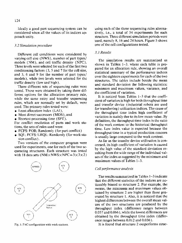
Fig. 5. FAC configuration with work stations.

using each of the three sequencing rules altema- tively, i.e., a total of 54 experiments for each structure. Three different simulation periods were used, namely 8, 16 and 24 hours. Figure 5 shows one of the cell con~gurations tested.

3.3 Results

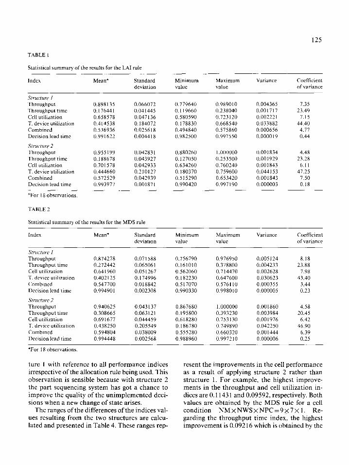
The simulation results are summarized as shown in Tables 1-3, where each table is prepared for an ahocation rule, showing an overail statistical summary of the performance indices over the eighteen experiments for each of the two structures. The tables include beside the mean and standard deviation the following statistics: minimum and maximum values, variance, and the coefficient of variation.

It is noticed from Tables l-3 that the coefli- cient of variation is high for both throughput time and transfer device (industrial robots are used for transfe~ing) utilization indices. The cause of the throughput time index high coefficient of variation is mainly due to its low mean value. By definition, the throughput time index is the ratio of the work content to the historical throughput time. Low index value is expected because the throughput time in a typical production concern is usually large compared to the work content.

As far as the transfer device utilization is concerned, its high coefficient of variation is caused by the high value of the standard deviation resulting from the wide range of the individual values of the index as suggested by the minimum and maximum values of Tables 1-3.

The results summarized in Tables l-3 indicate that the different statistics of the indices are no- ticeably biased to structure 2. For example, the means, the minimum and maximum values obtained by structure 2 are higher than those generated by structure 1. Also, it is noticed that the highest differences between the overall mean values of the two structures are produced by the throughput index (difference ranges between 0.057 and 0.066), while the lowest differences are obtained by the throughput time index (difference ranges between 0.012 and 0.036).

It is found that structure 2 outperforms struc-

125

TABLE 1

Statistical summary of the results for the LA1 rule

Index Mean’ Standard deviation

Minimum

value

Maximum

value

Variance Coefficient

of variance

Structure I Throughput

Throughput time

Cell utilization

T. device utilization

Combined

Decision lead time

Structure 2

Throughput

Throughput time

Cell utilization


Combined

Decision lead time

0.898 135 0.066072 0.779640 0.989010 0.004365 7.35

0.176441 0.041445 0.119660 0.238040 0.001717 23.49

-0.658578 0.047 I36 0.580590 0.723120 0.00222 1 7.15

0.414538 0.184072 0.178830 0.668540 0.033882 44.40

0.536936 0.025618 0.494840 0.575860 0.000656 4.77

0.991622 0.004418 0.982500 0.997550 0.000019 0.44

0.955199 0.04283 1 0.880260 I .oooooo 0.001834 4.48

0.188678 0.043927 0.127050 0.253500 0.001929 23.28

0.701578 0.042933 0.634260 0.760240 0.001843 6.1 1

0.444660 0.210127 0.180370 0.759600 0.044153 47.25

0.572529 0.042939 0.515290 0.653420 0.001843 7.50

0.993977 0.001871 0.990420 0.997190 0.000003 0.18

*For 18 observations.

TABLE 2

Statistical summary of the results for the MDS rule

Index Mean* Standard

deviation

Minimum

value

Maximum

value

Variance Coefficient

of variance

Structure 1 Throughput

Throughput time

Cell utilization


Combined

Decision lead time

Structure 2 Throughput

Throughput time

Cell utilization


Combined

Decision lead time

0.874278 0.071588 0.756790 0.976950 0.005 I24 8.18

0.272442 0.065061 0.161010 0.378800 0.004233 23.88

0.641960 0.05 1267 0.562060 0.714470 0.002628 7.98

0.402125 0.174996 0.182230 0.647600 0.030623 43.40

0.547700 0.018842 0.517070 0.576110 0.000355 3.44

0.994901 0.002308 0.990330 0.998010 0.000005 0.23

0.940625 0.043 137 0.867680 1 .oooooo 0.001860 4.58

0.308665 0.063121 0.195800 0.393230 0.003984 20.45

0.691677 0.044459 0.618280 0.753130 0.001976 6.42

0.438250 0.205549 0.186780 0.749890 0.042250 46.90

0.594804 0.038009 0.555280 0.660320 0.001444 6.39

0.994448 0.002568 0.988960 0.997210 0.000006 0.25

*For 18 observations

ture 1 with reference to all performance indices irrespective of the allocation rule being used. This observation is sensible because with structure 2 the part sequencing system has got a chance to improve the quality of the unimplemented decisions when a new change of state arises.

The ranges of the differences of the indices values resulting from the two structures are calcu- lated and presented in Table 4. These ranges rep-

resent the improvements in the cell performance as a result of applying structure 2 rather than structure 1. For example, the highest improvements in the throughput and cell utilization indices are 0.1143 1 and 0.09592, respectively. Both values are obtained by the MDS rule for a cell condition NMxNWSXNPC=~X~X 1. Re- garding the throughput time index, the highest improvement is 0.092 16 which is obtained by the

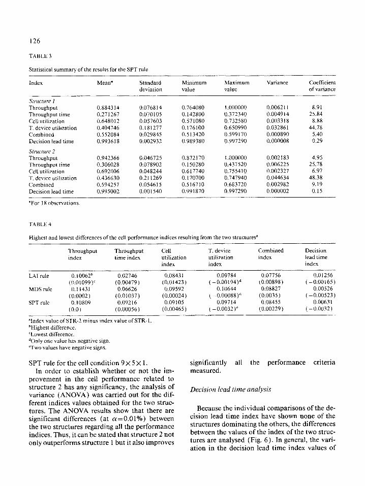
126

TABLE 3

Statistical summary of the results for the SPT rule

Index Mean* Standard deviation

Minimum value

Maximum value

Variance Coefficient of variance

Structure 1 Throughput Throughput time Cell utilization T. device utilization Combined Decision lead time

S~~u~~~re 2 Throughput Throughput time Cell utilization T. device utilization Combined Decision lead time - *For 18 observations.

0.884314 0.076814 0.764080 1 .oooooo 0.0062 11 8.91 0.271267 0.070105 0.142800 0.372340 0.0049 I4 25.84 0.648012 0.057603 0.571080 0.732580 0.003318 8.88 0.404146 0.181277 0.176100 0.650990 0.032861 44.78 0.552084 0.029845 0.513420 0.599170 0.000890 5.40 0.993618 0.002932 0.989380 0.997290 0.000008 0.29

0.942366 0.046725 0.872170 1 .oooooo 0.002 183 4.95 0.306028 0.078902 0.150280 0.437520 0.006225 25.78 0.692006 0.048244 0.617740 0.755410 0.002327 6.97 0.436630 0.211269 0.170700 0.747940 0.044634 48.38 0.594257 0.054615 0.516710 0.683720 0.002982 9.19 0.995002 0.001540 0.991870 0.997290 0.000002 0.15

TABLE 4

Highest and lowest differences of the cell performance indices resulting from the two structuresa

Throughput Throughput index time index

LA1 rule

MDS rule

SPT rule

0. 10062b 0.02746 0.0843 1 0.09784 0.07756 0.012S6 (0.01099)’ (0.00479 ) (0.01423) (-0.00194)d (0.00898) (-0.00166) 0.11431 0.06626 0.09592 0.10644 0.08827 0.00526

(0.0002) (0.01037) (0.00024) (-0.00088)d (0.0035) (-0.00523) 0.10809 0.09216 0.09105 0.09714 0.08455 0.0063 1

(0.0) (0.00056) (0.00465) (-0.0032)’ (0.00229) ( - 0.0032)

Cell T. device utilization utilization index index

Combined index

Decision lead time index

“Index value of STR-2 minus index value of STR-1 bHighest difference. ‘Lowest difference. “Only one value has negative sign. ‘Two values have negative signs.

SPT rule for the cell condition 9 X 5 X 1. In order to establish whether or not the im-

provement in the cell performance related to structure 2 has any significancy, the analysis of variance (ANOVA) was carried out for the different indices values obtained for the two structures. The ANOVA results show that there are significant differences (at CY = 0.01% ) between the two structures regarding all the performance indices. Thus, it can be stated that structure 2 not only outperforms structure 1 but it also improves

significantly all the performance criteria measured.

Decision lead time analysis

Because the individual comparisons of the decision lead time index have shown none of the structures dominating the others, the differences between the values of the index of the two strnc- tures are analysed (Fig. 6 ). In general, the variation in the decision lead time index values of

127

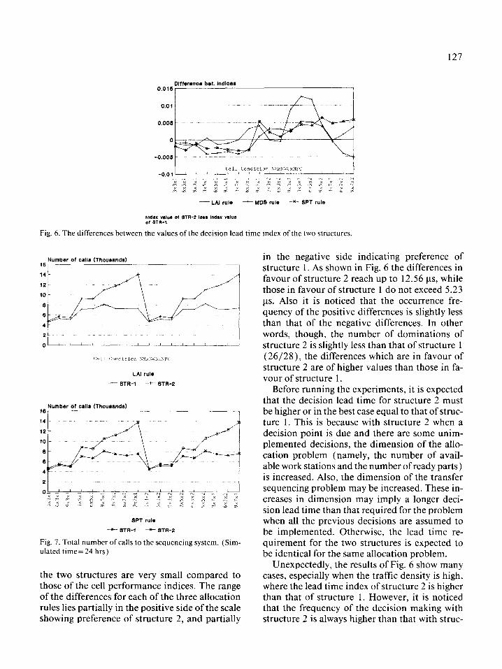
DIfferonce bet. Indioea 0.016

Fig. 6. The differences between the values of the decision lead time index of the two structures.

Number of oallb (Thousands) 161.

LAI rula

- STR-1 + STR-2

Number of caII1) (Thousands) 161

SPT rule

- STR-1 - STA-2

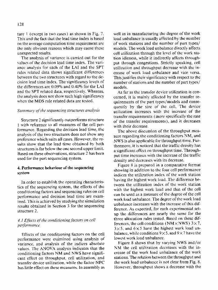
Fig. 7. Total number of calls to the sequencing system. (Sim- ulated time= 24 hrs)

the two structures are very small compared to those of the cell performance indices. The range of the differences for each of the three allocation rules lies partially in the positive side of the scale showing preference of structure 2, and partially

in the negative side indicating preference of structure 1. As shown in Fig. 6 the differences in favour of structure 2 reach up to 12.56 us, while those in favour of structure 1 do not exceed 5.23 us. Also it is noticed that the occurrence frequency of the positive differences is slightly less than that of the negative differences. In other words, though, the number of dominations of structure 2 is slightly less than that of structure 1 (26/28), the differences which are in favour of structure 2 are of higher values than those in favour of structure 1.

Before running the experiments, it is expected that the decision lead time for structure 2 must be higher or in the best case equal to that of structure 1. This is because with structure 2 when a decision point is due and there are some unimplemented decisions, the dimension of the allocation problem (namely, the number of available work stations and the number of ready parts) is increased. Also, the dimension of the transfer sequencing problem may be increased. These increases in dimension may imply a longer decision lead time than that required for the problem when all the previous decisions are assumed to be implemented. Otherwise, the lead time requirement for the two structures is expected to be identical for the same allocation problem.

Unexpectedly, the results of Fig. 6 show many cases, especially when the traffic density is high, where the lead time index of structure 2 is higher than that of structure 1. However, it is noticed that the frequency of the decision making with structure 2 is always higher than that with struc-

128

ture 1 (except in two cases) as shown in Fig. 7. This and the fact that the lead time index is based on the average computation time requirement are the only obvious reasons which may cause these unexpected results.

The analysis of variance is carried out for the values of the decision lead time index. The variance analysis for each of the LA1 and the SPT rules related data shows significant differences between the two structures with regard to the decision lead time index. The signi~cancy levels of the differences are 0.09% and 0.40% for the LA1 and the SPT related data, respectively. Whereas, the analysis does not show such high significancy when the MDS rule related data are tested.

Summary of the sequencing structures analysis

Structure 2 signi~cantly outperforms structure I with reference to all measures of the cell performance. Regarding the decision lead time, the analysis of the two st~~tures does not show any preference which suits all cases. However, the results show that the lead time obtained by both structures is far below the one second upper limit. Based on these observations, structure 2 has been used for the part sequencing system.

4. Performance behaviour of the sequencing system

In order to establish the operating characteris- tics of the sequencing system, the effects of the conditioning factors and sequencing rules on cell performance and decision lead time are examined. This is achieved by studying the simulation results obtained in Section 3 for the sequencing structure 2.

4. I Effects qf the conditioning factors on cell pe[formance

Effects of the conditioning factors on the cell performance were examined using analysis of variance, and analysis of the indices absolute values. The ANOVA analysis indicates that the conditioning factors NM and NWS have significant effect on throughput, cell utilization, and transfer device utilization, while the factor NPC has little effect on these measures. In assembly as

well as in manufacturing the degree of the work load unbalance is usually affected by the number of work stations and the number of part types/ models. The work load unbalance directly affects cell utilization through the level of the work station idleness, while it indirectly affects throughput through congestions. Strictly speaking, cell utilization and throughput decrease with the increase of work load unbalance and vice versa. This justifies their signiftcancy with respect to the number of stations and the number of part types/ models.

As far as the transfer device utilization is concerned, it is mainly affected by the transfer requirements of the part types/models and consequently by the size of the cell. The device utilization increases with the increase of the transfer requirements (more specifically the rate of the transfer requirements), and it decreases with their decrease.

The above discussion of the throu~put measure regarding the conditioning factors NM, and NWS is also applicable for throughput time. Fur- thermore, it is noticed that the traffic density has a significant effect on throughput time. Through- put time increases with the increase of the traffic density and decreases with its decrease.

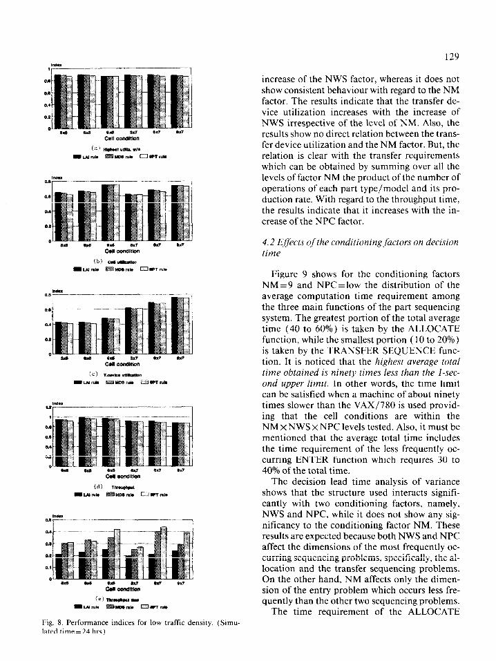
Figure 8 is prepared in a comparative format showing in addition to the four cell performance indices the utilization index of the work station having the highest work load, The difference between the utilization index of the work station with the highest work load and that of the cell can be used as a measure of the degree of the cell work load unbalance. The degree of the work load unbalance increases with the increase of this difference. As expected, for each experimental set- up the differences are nearly the same for the three allocation rules tested. Based on these differences, the cell conditions (NM x NWS) 3 x 7, 3 x 5, and 6 x 5 have the highest work load unbalance, while conditions 9 x 5, and 9 x 7 have the lowest work load unbalance.

Figure 8 shows that by varying NWS and/or NM the cell utilization decreases with the increase of the work load unbalance of the work stations. The relation between the throughput and the work load unbalance is not clear from Fig. 8. However, throu~put shows a decrease with the

129

krdu ‘J, I

1 ___. __ .-.

ab

0.b

M

QI

0

Fig. 8. Performance indices for low traffk density. (Simu- lated time=24 hrs)

increase of the NWS factor, whereas it does not show consistent behaviour with regard to the NM factor. The results indicate that the transfer device utilization increases with the increase of NWS irrespective of the level of NM. Also, the results show no direct relation between the transfer device utilization and the NM factor. But, the relation is clear with the transfer requirements which can be obtained by summing over all the levels of factor NM the product of the number of operations of each part type/model and its production rate. With regard to the throughput time, the results indicate that it increases with the increase of the NPC factor.

4.2 Effects of the conditioning factors on decision time

Figure 9 shows for the conditioning factors NM= 9 and NPC=low the distribution of the average computation time requirement among the three main functions of the part sequencing system. The greatest portion of the total average time (40 to 60%) is taken by the ALLOCATE function, while the smallest portion ( 10 to 20%) is taken by the TRANSFER SEQUENCE function. It is noticed that the highest average total time obtained is ninety times less than the l-second upper limit. In other words, the time limit can be satisfied when a machine of about ninety times slower than the VAX/780 is used providing that the cell conditions are within the NM x NWS x NPC levels tested. Also, it must be mentioned that the average total time includes the time requirement of the less frequently oc- curring ENTER function which requires 30 to 40% of the total time.

The decision lead time analysis of variance shows that the structure used interacts significantly with two conditioning factors, namely, NWS and NPC, while it does not show any sig- nilicancy to the conditioning factor NM. These results are expected because both NWS and NPC affect the dimensions of the most frequently oc- curring sequencing problems, specifically, the allocation and the transfer sequencing problems. On the other hand, NM affects only the dimension of the entry problem which occurs less frequently than the other two sequencing problems.

The time requirement of the ALLOCATE

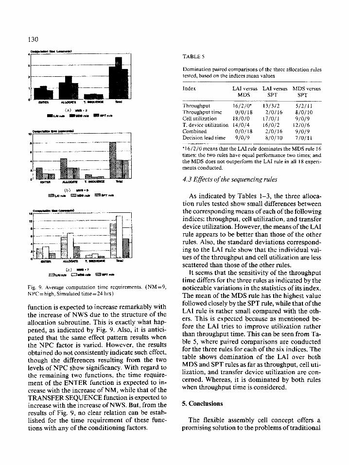
Fig. 9. Average computation time requirements. (NM=9, NPC = high, Simulated time = 24 hrs)

function is expected to increase remarkably with the increase of NWS due to the structure of the allocation subroutine. This is exactly what hap- pened, as indicated by Fig. 9. Also, it is antici- pated that the same effect pattern results when the NPC factor is varied. However, the results obtained do not consistently indicate such effect, though the differences resulting from the two levels of NPC show significancy. With regard to the remaining two functions, the time requirement of the ENTER function is expected to increase with the increase of NM, while that of the TRANSFER SEQUENCE function is expected to increase with the increase of NWS. But, from the results of Fig. 9, no clear relation can be established for the time requirement of these functions with any of the conditioning factors.

TABLE 5

Domination paired comparisons of the three allocation rules tested, based on the indices mean values

Index LA1 versus LA1 versus MDS versus MDS SPT SPT

Throughput 16/2/o* 13/3/2 5/2/l I Throughput time O/O/18 2/O/16 8/O/10 Cell utilization 18/O/O 17/O/l 9/o/9 T. device utilization 14/O/4 16/O/2 12/O/6 Combined O/O/18 2/O/16 9/o/9 Decision lead time 9/o/9 s/o/10 7/O/l 1

*16,/2/O means that the LA1 rule dominates the MDS rule 16 times; the two rules have equal performance two times; and the MDS does not outperform the LA1 rule in all 18 experiments conducted.

4.3 Effects of the sequencing rules

As indicated by Tables 1-3, the three allocation rules tested show small differences between the corresponding means of each of the following indices: throughput, cell utilization, and transfer device utilization. However, the means of the LA1 rule appears to be better than those of the other rules. Also, the standard deviations corresponding to the LA1 rule show that the individual values of the throughput and cell utilization are less scattered than those of the other rules.

It seems that the sensitivity of the throughput time differs for the three rules as indicated by the noticeable variations in the statistics of its index. The mean of the MDS rule has the highest value followed closely by the SPT rule, while that of the LA1 rule is rather small compared with the others. This is expected because as mentioned before the LA1 tries to improve utilization rather than throughput time. This can be seen from Ta- ble 5, where paired comparisons are conducted for the three rules for each of the six indices. The table shows domination of the LA1 over both MDS and SPT rules as far as throughput, cell utilization, and transfer device utilization are concerned. Whereas, it is dominated by both rules when throu~put time is considered.

5. Conclusions

The flexible assembly cell concept offers a promising solution to the problems of traditional

mixed-model and multi-product assembly lines of small and medium-sized products. A totally computerized real time part sequencing system is developed for controlling the part flow in these cells. Development of the sequencing structure of the system has been established through a series of simulation studies using different types of in- put data. The control functions of the system are provided with different priority options enabling the user to select the set of rules which satisfies his company strategy.

The performance behaviour of the system developed has been examined under different cell conditions and sequencing rules. The results of the examination can be summarized in the following: l The ANOVA analysis shows that

- The conditioning factors NM and NWS have significant effect on throughput, cell utilization, and transfer device utilization, while the factor NPC has little effect on these measures.

- The throughput time is significantly affected by the three conditioning factors examined, i.e., NM, NWS, and NPC. l From the analysis of the indices’ absolute

values, it is noticed that By varying NWS and/or NM the cell utilization decreases with the increase of the work load unbalance of the work stations. The transfer device utilization increases with the increase of NWS irrespective of the level of NM. The throughput decreases with the increase of the NWS factor. The throughput time increases with the increase of the NPC factor. a The effects of the sequencing rules on per-

formance show that - The non-model-file related priority rule LA1

outperforms both MDS and SPT rules with respect to throughput, cell utilization, and transfer device utilization, whereas it is being out- performed by both rules with regard to throughput time. l The analysis of the decision lead time shows

that - The greatest portion of the total average time

(40 to 60%) is taken by the ALLOCATE function, while the smallest portion ( 10 to 20%) is

131

taken by the TRANSFER SEQUENCE function.

- The l-second time limit can be satisfied when a machine of about ninety times slower than the VAX/780 is used providing that the cell conditions are within the NM x NWS x NPC levels tested.

- The conditioning factors NWS and NPC have significant effect on the decision lead time.

- The time requirement of the ALLOCATE function increases considerably with the increase of NWS.

References

1

2

3

4

5

6

7

8

9

10

11

12

Warnecke, H.J. and Walther, J., 1982. Automatic assembly state-of-the-art, Proc. 3rd Int. Conf. Assembly Automation and 14th IPA Conf., Boeblingen, W. Ger- many, pp. I-14. Ramesh, R. and Gary, J.M., 1989. Multicriteria jobshop scheduling. Comput. Ind. Eng., 17 ( l-4): 597-602. Suliman, S.M.A., Al-Tamimi, A.M. and Nawara, G.M., 1985. Computational methods for the mixed-model assembly line problem: a review. J. Eng. Sci., 11 (2): 241- 271. Abdallah, H.M., 1973. Computer simulation studies for a heuristic scheduling system. Ph.D. Thesis, Crantield Institute of Technology, UK. Blackstone, J.H., Phillips, D.T. and Hogg, G.L., 1982. A state-of-the-art survey of dispatching rules for manufac- turingjob shop operation. Int. J. Prod. Res., 20 ( 1): 27- 45. Choi, R.H. and Malstrom, E.M., 1988. Evaluation of traditional work scheduling rules in a flexible manufacturing system with a physical simulator. J. Manuf. Sys., 7 ( 1): 33-45. Conway, R.W., Maxwell, W.L. and Miller, L.W., 1967. Theory of scheduling. Addison Wesley, Reading, MA, USA. Gere, W., 1966. Heuristics in job shop scheduling. Man- age. Sci., 13 (3): 167-190. Panwalker, S.S. and Iskander, W., 1977. A survey of scheduling rules. Oper. Res., 25 ( 1 ): 45-6 1. Aanen, E., Gaalman, G.J. and Nawijn, W.M., 1989. Planning and scheduling in an FMS. Eng. Costs Prod. Econ., 17 (l-4): 89-97. Suliman, S.M.A., 1987. An investigation into part sequencing in a flexible assembly cell. Ph.D. Thesis, Cran- field Institute of Technology, UK. Williams, D.F., El-Tamimi, A.M. and Suliman, S.M.A., 1987. Product selection and investment appraisal for flexible assembly, Proc. Inst. Mech. Eng., 201 (Bl ).

Documents

Real-time part sequencing in a flexible assembly cell: system development and evaluation