Embed Size (px)
Citation preview

Real time segmentation of heart sounds.
by
David Fourie
Thesis presented in partial fulfilment of the requirements forthe degree of Master of Engineering (Electrical) in the
Faculty of Engineering at Stellenbosch University
Supervisor: Dr. M.J. Booysen
December 2015

Declaration
By submitting this thesis electronically, I declare that the entirety of the workcontained therein is my own, original work, that I am the sole author thereof(save to the extent explicitly otherwise stated), that reproduction and pub-lication thereof by Stellenbosch University will not infringe any third partyrights and that I have not previously in its entirety or in part submitted it forobtaining any qualification.
2015/12/10Date: . . . . . . . . . . . . . . . . . . . . . . . . . . . . . . .
Copyright © 2015 Stellenbosch UniversityAll rights reserved.
i
Stellenbosch University https://scholar.sun.ac.za

Abstract
Real time segmentation of heart sounds.D. Fourie
Department of Electrical and Electronic Engineering,University of Stellenbosch,
Private Bag X1, Matieland 7602, South Africa.
Thesis: MEng (Elec)September 2015
The poor state of the healthcare system in South Africa has resulted in un-acceptable high levels of infant mortality. Congenital heart disease is one ofthe main contributions to these high rates of mortality, with the cost of treat-ment and the availability of specialists being the driving factors. Computeraided auscultation is a technological solution to assist with the diagnosis ofthe disease. In its current form, computer aided auscultation is unsuitable forcontinuous patient monitoring.
The aim of this thesis is to develop an algorithm that will allow the existingmethods of computer aided auscultation to work in real time so they canbe used in patient monitoring. Existing methods of identifying the first andsecond heart sound are limited to offline processing. The algorithm developedin this thesis uses the correlation of the time-frequency coefficients of individualheart sounds to generate a feature vector for each heart sound that can beused to separate the sounds into different groups. To test the performanceof the algorithm, 230 heart sounds from normal patients were first manuallysegmented and then processed with the algorithm. The noise sensitivity of thealgorithm was also tested using generated heart sounds. Finally, the real timecapability of the algorithm was tested.
The testing against sounds form normal patients resulted in a 84.2 % ac-curacy and an 84.4% hit rate. The synthetic testing showed the system startsto perform badly with a signal to noise ratio lower than -10db. The real timetesting of the system showed that the algorithm is fast enough to be used ina real time environment. This thesis concludes that proposed algorithm issuitable for the detection of the first and second heart sounds in real time.
ii
Stellenbosch University https://scholar.sun.ac.za

UittrekselIntydse segmentering van hartklanke
D. FourieDepartement van Elektriese en Elektroniese Ingenieurswese,
Universiteit van Stellenbosch,Privaatsak X1, Matieland 7602, Suid Afrika.
Tesis: MIng (Elek)September 2015
Die toestand van die gesondheidstelsel in Suid-Afrika lei tot onaanvaarbarevlakke van kindersterftes. Oorerflike hartksiektes is een van die hoofoorsakevan hierdie sterftesyfers, aangedryf deur die koste van behandeling en die te-kort aan beskikbaarheid van spesialiste. Rekenaargesteundebeluistering is ’ntegnologiese oplossing wat help met die diagnose van hierdie kwaal. Huidiglikis rekenaargesteundebeluistering ongeskik vir aaneenlopende pasientemonite-ring.
Die doelwit van hierdie tesis in om ’n algoritme te onwikkel wat sal toe-laat dat bestaande metodes van rekenaargestuendebeluistering intyds sal werksodat gebruik kan word vir deurlopende monitering van pasiente. Bestaandemetodes, wat aangewend word om die eerste- en tweede hartklanke te identi-fiseer, is beperk tot nie-intydse verwerking. Die algoritme wat in hierdie tesisontwikkel is, gebruik die korrelasie van die tyd-frekwensie koeffisiente van in-dividuele hartklanke om ’n eienskapsvektor vir elke hartklank te genereer, watdan gebruik word om die hartklanke in verskillende groepe in te deel. Omdie werkverrigting van die algoritme te toets, is 230 hartklanke van pasientemet normale harte eers per hand gesegmenteer en daarna met die algoritmeverwerk. Die algoritme se bestandheid teen ruis is ook getoets deur gebruikte maak van sintetiese hartklanke. Uiteindelik is die intydse vermoë van diealgortime getoets.
Die toetsing met normale hartklanke het ’n akkuraatheid van 84.2% en tref-koers van 84.4% opgelewer. Die ruisbestandheidstoetse het aangedui dat diestelsel sleg begin werkverrigting verloor met sein-tot-ruis-verhoudings van laeras -10dB. Die intydse toetsing het aangedui dat die algoritme vining genoeg isom gebruik te word in ’n intydse implementering. Die tesis maak die gevolg-trekking dat die voorgestelde algoritme geskik is vir die intydse identifiseringvan die eerste en tweede hartklanke.
iii
Stellenbosch University https://scholar.sun.ac.za

Acknowledgements
I would like to express my sincere gratitude to the following people and organ-isations who have contributed to making this work possible;
• Dr. M.J. Booysen for his invaluable and patient support as study leader.
• Thys Cronje and Eugene Pretorius from Diacoustic medical devices fortheir financial support and useful guidance.
• My colleagues and the staff in the Electronic Systems Lab for accom-modating a project that is completely different to the usual work of thelab.
• My family for their continuous encouragement.
iv
Stellenbosch University https://scholar.sun.ac.za

Contents
Declaration i
Abstract ii
Uittreksel iii
Acknowledgements iv
Contents v
List of Figures vii
List of Tables x
Nomenclature xi
1 Introduction 11.1 South African context . . . . . . . . . . . . . . . . . . . . . . . 21.2 Cardiac Auscultation . . . . . . . . . . . . . . . . . . . . . . . . 31.3 Research gap . . . . . . . . . . . . . . . . . . . . . . . . . . . . 31.4 Thesis statements and hypotheses . . . . . . . . . . . . . . . . . 41.5 Thesis overview . . . . . . . . . . . . . . . . . . . . . . . . . . . 4
2 Literature review 52.1 Cardiovascular system . . . . . . . . . . . . . . . . . . . . . . . 52.2 Heart sounds . . . . . . . . . . . . . . . . . . . . . . . . . . . . 62.3 Cardiovascular disease detectable with auscultation . . . . . . . 82.4 Existing methods for cardiac auscultation . . . . . . . . . . . . 9
3 Development 133.1 Enveloping methods . . . . . . . . . . . . . . . . . . . . . . . . 133.2 Peak detection . . . . . . . . . . . . . . . . . . . . . . . . . . . 183.3 Time frequency methods . . . . . . . . . . . . . . . . . . . . . . 193.4 Statistical clustering . . . . . . . . . . . . . . . . . . . . . . . . 263.5 Summary . . . . . . . . . . . . . . . . . . . . . . . . . . . . . . 26
v
Stellenbosch University https://scholar.sun.ac.za
CONTENTS vi
4 Method 274.1 Inspiration for method . . . . . . . . . . . . . . . . . . . . . . . 274.2 Algorithm . . . . . . . . . . . . . . . . . . . . . . . . . . . . . . 274.3 Synthetic testbed . . . . . . . . . . . . . . . . . . . . . . . . . . 324.4 Summary . . . . . . . . . . . . . . . . . . . . . . . . . . . . . . 37
5 Testing 385.1 Offline testing . . . . . . . . . . . . . . . . . . . . . . . . . . . . 385.2 Synthetic testing . . . . . . . . . . . . . . . . . . . . . . . . . . 405.3 Online testing . . . . . . . . . . . . . . . . . . . . . . . . . . . . 535.4 Summary . . . . . . . . . . . . . . . . . . . . . . . . . . . . . . 53
6 Conclusion 54
Bibliography 55
Stellenbosch University https://scholar.sun.ac.za
List of Figures
1.1 Figure showing the causes of mortality in children under 5 [1] . . . 2
2.1 Diagram showing the movement of blood through the cardiovascu-lar system [2] . . . . . . . . . . . . . . . . . . . . . . . . . . . . . . 6
2.2 Diagram showing the anatomy of the heart [2] . . . . . . . . . . . . 7
3.1 Graph showing the Hilbert envelope of a signal segment . . . . . . . 143.2 Graph showing the Homomorphic envelope of a signal segment us-
ing a lowpass filter of 5 Hz . . . . . . . . . . . . . . . . . . . . . . . 153.3 Graph showing the Homomorphic envelope of a signal segment us-
ing a lowpass filter of 10 Hz . . . . . . . . . . . . . . . . . . . . . . 153.4 Graph showing the Homomorphic envelope of a signal segment us-
ing a lowpass filter of 20 Hz . . . . . . . . . . . . . . . . . . . . . . 163.5 Graph showing the comparison of the different types of energy
transforms. . . . . . . . . . . . . . . . . . . . . . . . . . . . . . . . 173.6 Graph showing the effect of N = 5 on the Shannon Envelope. . . . 173.7 Graph showing the effect of N = 10 on the Shannon Envelope. . . . 173.8 Graph showing the effect of N = 20 on the Shannon Envelope. . . . 183.9 Graph showing the effect of ω0 = π on scaling functions for different
frequencies . . . . . . . . . . . . . . . . . . . . . . . . . . . . . . . . 213.10 Graph showing the effect of ω0 = 5π on scaling functions for differ-
ent frequencies . . . . . . . . . . . . . . . . . . . . . . . . . . . . . 213.11 Contour plot showing the effect of ω0 = π on the CWT of heart
sounds . . . . . . . . . . . . . . . . . . . . . . . . . . . . . . . . . . 223.12 Contour plot showing the effect of ω0 = 5π on the CWT of heart
sounds . . . . . . . . . . . . . . . . . . . . . . . . . . . . . . . . . . 223.13 Block diagram of one level in a DWT filter bank. . . . . . . . . . . 233.14 Block diagram of three levels of a DWT filterbank. . . . . . . . . . 233.15 2D heatmap of the distribution of DWT coefficients for the db6
wavelet. . . . . . . . . . . . . . . . . . . . . . . . . . . . . . . . . . 243.16 2D heatmap of the distribution of DWT coefficients for the db3
wavelet. . . . . . . . . . . . . . . . . . . . . . . . . . . . . . . . . . 243.17 Figure showing a frequency sweep from 5 Hz to 15 Hz . . . . . . . 253.18 Plot showing the instantaneous frequency content of heart sounds . 26
vii
Stellenbosch University https://scholar.sun.ac.za

LIST OF FIGURES viii
4.1 Flow diagram showing the layout of the S1 - S2 detection system . 284.2 Graph showing the Envelope, PCG and identified peaks. . . . . . . 284.3 Graph showing wavelet coefficients of the signal. . . . . . . . . . . . 294.4 Graph showing transformed wavelet coefficients of the signal. . . . . 294.5 Graph showing the correlation of the transformed wavelet coefficients. 304.6 Graph showing the grouped correlations of the signal. . . . . . . . . 304.7 Flow diagram showing the layout of the real time system . . . . . . 314.8 Graphs showing the original signal and the first approximation. . . 334.9 Graphs showing the original signal and the second approximation. . 344.10 Graphs showing the original signal and the third approximation. . . 344.11 Graphs showing the original signal and the final approximation. . . 354.12 Graph showing a 60 BPM generated heart signal. . . . . . . . . . . 364.13 Graph showing a 90 BPM generated heart signal. . . . . . . . . . . 364.14 Graph showing a 120 BPM generated heart signal. . . . . . . . . . 36
5.1 Graph showing a generated signal with uncorrelated noise with aSNR of -50dB. . . . . . . . . . . . . . . . . . . . . . . . . . . . . . 41
5.2 Graph showing a generated signal with uncorrelated noise with aSNR of -15dB. . . . . . . . . . . . . . . . . . . . . . . . . . . . . . 42
5.3 Graph showing a generated signal with uncorrelated noise with aSNR of 5dB. . . . . . . . . . . . . . . . . . . . . . . . . . . . . . . . 42
5.4 Graph showing the relationship between SNR and performance at60 BPM. . . . . . . . . . . . . . . . . . . . . . . . . . . . . . . . . . 43
5.5 Graph showing the relationship between SNR and performance at90 BPM . . . . . . . . . . . . . . . . . . . . . . . . . . . . . . . . . 44
5.6 Graph showing the relationship between SNR and performance at120 BPM. . . . . . . . . . . . . . . . . . . . . . . . . . . . . . . . . 45
5.7 Graph showing a generated signal with correlated noise with a SNRof -50dB. . . . . . . . . . . . . . . . . . . . . . . . . . . . . . . . . 45
5.8 Graph showing a generated signal with correlated noise with a SNRof -15dB. . . . . . . . . . . . . . . . . . . . . . . . . . . . . . . . . 46
5.9 Graph showing a generated signal with correlated noise with a SNRof 5dB. . . . . . . . . . . . . . . . . . . . . . . . . . . . . . . . . . . 46
5.10 Graph showing the relationship between SNR and performance at60 BPM. . . . . . . . . . . . . . . . . . . . . . . . . . . . . . . . . . 47
5.11 Graph showing the relationship between SNR and performance at90 BPM. . . . . . . . . . . . . . . . . . . . . . . . . . . . . . . . . . 48
5.12 Graph showing the relationship between SNR and performance at120 BPM. . . . . . . . . . . . . . . . . . . . . . . . . . . . . . . . . 49
5.13 Graph showing a generated signal with correlated noise with a SNRof -50dB. . . . . . . . . . . . . . . . . . . . . . . . . . . . . . . . . 49
5.14 Graph showing a generated signal with correlated noise with a SNRof -15dB. . . . . . . . . . . . . . . . . . . . . . . . . . . . . . . . . 50
Stellenbosch University https://scholar.sun.ac.za

LIST OF FIGURES ix
5.15 Graph showing a generated signal with correlated noise with a SNRof 5dB. . . . . . . . . . . . . . . . . . . . . . . . . . . . . . . . . . . 50
5.16 Graph showing the relationship between SNR and performance at60 BPM. . . . . . . . . . . . . . . . . . . . . . . . . . . . . . . . . . 51
5.17 Graph showing the relationship between SNR and performance at90 BPM. . . . . . . . . . . . . . . . . . . . . . . . . . . . . . . . . . 52
5.18 Graph showing the relationship between SNR and performance at120 BPM. . . . . . . . . . . . . . . . . . . . . . . . . . . . . . . . . 53
Stellenbosch University https://scholar.sun.ac.za

List of Tables
2.1 Table highlighting the contribution of this work against the stateof the art. . . . . . . . . . . . . . . . . . . . . . . . . . . . . . . . . 12
5.1 Table to show results of the system implemented in this thesis. . . . 38
x
Stellenbosch University https://scholar.sun.ac.za

Nomenclature
Medical abbreviationsCHD Congenital Heart diseaseVSD Ventricular Septal DefectASD Atrial Septal defectPDA Patent Ductus ArteriosusCAA Computer Aided AuscultationECG Electrocardiogram
Signal processing abbreviationsSTFT Short Time Fourier TransformCWT Continuous Wavelet TransformDWT Discrete Wavelet Transform
xi
Stellenbosch University https://scholar.sun.ac.za

Chapter 1
Introduction
Congenital heart disease (CHD) is the term for a range of conditions which arepresent in the heart at the time of birth. CHD has an incidence of 6/1000 livebirths for moderate to serious cases, and 60/1000 for all cases [3]. These ratesare estimated to be relatively constant for difference countries [3]. The mostcommon of these CHDs is the ventricular septal defect (VSD), patent ductusarteriosus (PDA) and the atrial septal defect (ASD) [3]. These conditions areusually identified by the murmur they produce during physical examination.This is problematic as heart murmurs occur in 80% of children, with the ma-jority of them being innocent [4]. This leads to high rates of false positiveswhen the patient is later examined with echocardiography [4]. The high ratesof false positives increases the workload of specialists [5] and increases parentalstress [6].
To address this problem of false positives, Computer Aided Auscultation(CAA) was developed to assist the primary care practitioner with the diagno-sis. CAA uses signal processing and machine learning techniques to analyse thesound signals that emanate from the heart. Using CAA, medical practitionersare able to reduce the incidents of false positives [7].
The longterm continuous assessment of patients is commonly done to con-firm the presence of a heart condition such as cardiac arrhythmia. Theseassessments are done using a portable device that records and analyses theElectrocardiogram (ECG) of the heart [8]. Whilst the ECG is capable of as-sessing certain conditions of the heart, it is unable to directly asses the move-ment of blood in the heart. This means that conditions such as PDA cannotbe monitored automatically with an ECG. This gap forms the part of the basisof this thesis.
1
Stellenbosch University https://scholar.sun.ac.za

CHAPTER 1. INTRODUCTION 2
1.1 South African contextSouth Africa’s healthcare system is not providing the level of care needed tothe majority of its citizens [9]. 55% of South Africans rely on the publichealthcare system for all their medical needs [10]. A system that is under-staffed, underfunded and overburdened [9]. The system has to cope with theside effects of poverty such as malnutrition, low birth weight and HIV/Aidsover and above the standard problems any healthcare system has to face suchas non-communicable diseases [9]. The state of the healthcare system in SouthAfrica is reflected in the mortality rates for children under 5 in Figure 1.1.
Figure 1.1: Figure showing the causes of mortality in children under 5 [1]
CHD in South Africa has an incidence of 0.6-0.8/1000 in liveborn children,which is about 11 000 per year [10]. CHD is a mostly treatable set of conditionswith an 85% survival rate if there is adequate and timeous medical intervention[10]. In South Africa, the chances of getting the required intervention arelow with only 25% of the children with CHD in South Africa receiving thetreatment they need. The lack of treatment means that 3000 children dieannually from CHD [10]. One of the reasons for this number is the numberof referrals only represents a fraction of the total number of cases due to thecondition being missed, misdiagnosed or identified too late [10].
Stellenbosch University https://scholar.sun.ac.za

CHAPTER 1. INTRODUCTION 3
1.2 Cardiac AuscultationThe method of auscultation was first practised during the Hippocratic period(460 to 370 BC). As the stethoscope was not invented yet, it was performedby a physician placing his/her ear to the patient’s body. As well as beinguncomfortable for the patient and physician, the sounds were difficult to hear.The development of the stethoscope by Laennec in 1816 enabled physiciansto hear the sounds which the body makes more clearly, as well as making theprocess more comfortable for both patient and physician. As a result of thesuccess of the stethoscope, auscultation is now part of the standard physicalexam that is performed by medical practitioners [11].
Auscultation is performed during the physical examination of a patient todiagnose the function of a particular organ of the body. In cardiac auscultation,there are a number of sounds which are of interest to a medical practitioner.The different sounds are elicited from the body by moving the stethoscope todifferent parts of the chest and moving the patient to different positions [12].
Auscultation requires years of training by medical practitioners to becomea useful tool for diagnosis. This combined with the increasing prevalenceof echocardiography has resulted in a decline in the skill [13]. The effect onhaving medical practitioners with a lower effectiveness in auscultation will be ahigher incidence of misdiagnosis and higher unnecessary cost for the healthcaresystem and patients.
1.3 Research gapComputer aided auscultation has not been extended to work in real time forpatient monitoring. In neonates with PDA for example there is a persistentmurmur that indicates the presence of abnormal blood flow in the heart [14].The monitoring of the condition is currently done using repeated echocar-diograms, which require expensive equipment and employment of specialists.This drives up the cost of healthcare, both to the state and the patient. Themurmur that is present in PDA is detectable with current offline auscultatorytechniques [15]. The existing methods are easily adaptable to real time oncethe segmentation of heart sounds can be performed in real time. This is thebasis for the research statements in this thesis.
Stellenbosch University https://scholar.sun.ac.za

CHAPTER 1. INTRODUCTION 4
1.4 Thesis statements and hypothesesThesis Statement 1:
Heart sounds can be segmented using short signals.
Hypothesis 1.1 The information in one heart sound is sufficient to tell itapart from another heart sound.
Hypothesis 1.2 A heart sound signal segmented with short signals is accu-rate.
Thesis Statement 2:Heart sounds can be segmented in real time.
Hypothesis 2.1 The information in one heart sound can be analysed in ashort amount of time.
1.5 Thesis overviewChapter 2 presents an overview of the cardiovascular system, the types of
sounds that medical practitioners look for during auscultation, a few ofthe conditions that are diagnosed with auscultation and an overview ofthe literature surrounding the process of computer aided auscultation.
Chapter 3 describes the signal processing and statistical methods used inthis thesis.
Chapter 4 describes the methods used to prove the thesis statements as wellas the testing procedure.
Chapter 5 documents how the methods were tested and their performance.
Chapter 6 concludes the work by validating the hypotheses in Chapter 1.
Stellenbosch University https://scholar.sun.ac.za

Chapter 2
Literature review
2.1 Cardiovascular systemThe cardiovascular system is the system in the body responsible for deliveringoxygen and removing carbon dioxide from the body. The organs and tissueswhich make up this system are the heart, the lungs and the blood vessels. Theheart is responsible for the movement of blood though the system, the lungsare responsible for oxygenating the blood and removing carbon dioxide andthe blood vessels are responsible for the transportation of blood. A diagramof this system is shown in Figure 2.1.
The focus of this thesis is the heart. The heart consists of two sides: theright side which is responsible for delivering de-oxygenated blood to the lungsand the left side which is responsible for delivering oxygenated blood to therest of the body. Each side consists of two separate chambers called atria andventricles. The atria are chambers in which blood collects from the the bodyand lungs. The ventricles are the chambers which contract and provide thepressure required to deliver blood to the rest of the body.
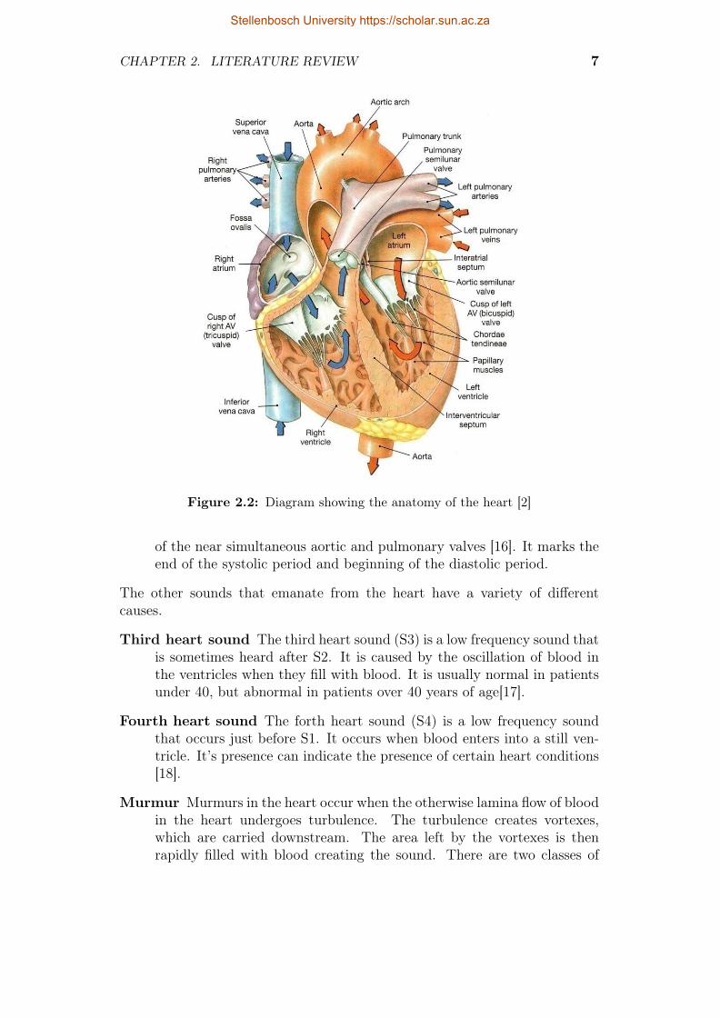
The atria and ventricles are connected by heart valves. The right atriumand ventricle are connected by the tricuspid valve and the left atrium andventricle are connected by the mitral valve. The valves ensure the blood flowsfrom the atria to the ventricles. The right ventricle is connected to the pul-monary artery via the pulmonary valve and the left ventricle is connected tothe aorta via the aortic valve [2] [12] [16].
The positions of these valves are shown in Figure 2.2.The path of blood through the heart explained below.
• The blood enters the heart through the vena cava and pulmonary vein.It fills the left and right atria.
• The atria contract and the blood enters the ventricles through the tri-cuspid and mitral valves.
5
Stellenbosch University https://scholar.sun.ac.za

CHAPTER 2. LITERATURE REVIEW 6
Figure 2.1: Diagram showing the movement of blood through the cardiovascularsystem [2]
• The ventricles contract and blood leaves the heart through the pul-monary and aortic valves into the pulmonary artery and aorta respec-tively.
2.2 Heart soundsThe two main sounds that emanate from the heart are caused by the rapiddeceleration of blood that occurs when the valves in the heart close. Thesesounds are listed below.
First heart sound The first heart sound (S1) consists of the superpositionof the sounds caused by the closing of the mitral and tricuspid valves. Itmarks the beginning of the systolic period and occurs when the ventriclescontract [12].
Second heart sound The second heart sound (S2) occurs after the first heartsound. It consists of the superposition of the sounds caused by the closing
Stellenbosch University https://scholar.sun.ac.za
CHAPTER 2. LITERATURE REVIEW 7
Figure 2.2: Diagram showing the anatomy of the heart [2]
of the near simultaneous aortic and pulmonary valves [16]. It marks theend of the systolic period and beginning of the diastolic period.
The other sounds that emanate from the heart have a variety of differentcauses.
Third heart sound The third heart sound (S3) is a low frequency sound thatis sometimes heard after S2. It is caused by the oscillation of blood inthe ventricles when they fill with blood. It is usually normal in patientsunder 40, but abnormal in patients over 40 years of age[17].
Fourth heart sound The forth heart sound (S4) is a low frequency soundthat occurs just before S1. It occurs when blood enters into a still ven-tricle. It’s presence can indicate the presence of certain heart conditions[18].
Murmur Murmurs in the heart occur when the otherwise lamina flow of bloodin the heart undergoes turbulence. The turbulence creates vortexes,which are carried downstream. The area left by the vortexes is thenrapidly filled with blood creating the sound. There are two classes of
Stellenbosch University https://scholar.sun.ac.za

CHAPTER 2. LITERATURE REVIEW 8
murmurs, ejection murmurs and regurgitation murmurs. Ejection mur-murs usually emanate from the aortic and pulmonary valves or the sur-rounding structures. Regurgitation murmurs occur when there is bloodflow in the wrong direction through a valve. Some ejection murmurs arenot indicative of a health condition and are innocent.
2.3 Cardiovascular disease detectable withauscultation
Some of the diseases that can be diagnosed with cardiac auscultation are listedbelow:
2.3.1 Atrial septal defect
An atrial septal defect is a congenital disease which causes blood to flow be-tween the atria. When the symptoms are present, they are typical of cardio-vascular disease (fatigue, exercise intolerance, shortness of breath). Howevermost childhood cases remain asymptomatic until adulthood [19]. Initial diag-nosis of an ASD is typically done using auscultation. The defect can causea persistent split in the second heart sound as well as a soft systolic ejectionmurmur [19].
2.3.2 Ventricular septal defect
A ventricular septal defect is a congenital disease which causes blood to flowbetween the ventricles. The defect, if small, causes no symptoms and may closeby itself. However if it is larger, it does cause symptoms which include fatigue,shortness of breath and exercise intolerance [20]. The diagnosis is typicallyperformed during the physical examination, with a pansystolic murmur beingthe primary indicator of the condition [20].
2.3.3 Valvular stenosis
Stenosis of the heart valves is the narrowing of the valve opening. This nar-rowing decreases the blood flow through the heart as well as increasing theworkload of the heart. These effects can cause the symptoms of exercise intol-erance and shortness of breath [21]. They also lead to further complicationsthat eventually cause heart failure. Aortic stenosis the most common form ofvalvular stenosis. The auscultatory signature of aortic stenosis is a systolicmurmur [21].
Stellenbosch University https://scholar.sun.ac.za
CHAPTER 2. LITERATURE REVIEW 9
2.3.4 Valvular regurgitation
Valvular regurgitation is flow of blood in the incorrect direction though a valve.This leads to an increase in the workload of the heart, which can eventually leadto heart failure [22]. The condition is initially asymptomatic, but eventuallyleads to heart failure if untreated. Mitral regurgitation is the most commonform of regurgitation. The auscultatory signature of mitral regurgitation is adiastolic murmur [22].
2.4 Existing methods for cardiac auscultationMost of the previous work in the field is related to the detection and identifica-tion of the first and second heart sounds in pre-recorded signals. This processis known as heart sound segmentation.There has been limited work done inthe segmentation of heart sounds in real time.
2.4.1 Offline segmentation
2.4.1.1 Segmentation with signal envelope
The most basic method of heart sound segmentation uses envelope detectionand physiological timing. The signal envelope is used to identify the location ofheart sounds in the signal. Once the locations of the hearts sounds are found,they are identified by using the physiological timing differences between thefirst and second heart sounds.
The different types of enveloping methods were tested in [23]. The methodswere successful in identifying the first and second heart sounds using theirtiming differences. The timing differences between the first and second heartsound decrease as the heart rate increases, thus this method is only suitablefor patients with a low heart rate.
2.4.1.2 Segmentation with Neural Networks
A time delay neural network was used to identify the first heart sound usingseries of feature vectors generated from the energy of a continuous wavelettransform in [24]. The method used the electrocardiogram to identify S1 peaksin the heart sound signal or phonocardiogram (PCG). The time delay neuralnetwork was then trained to identify these peaks from the wavelet features.This method was successful in that it could reliably identify S1 peaks basedsolely on their time-frequency content. The main advantage of this method isthat it can work on a short-time basis that could enable a system to performthe analysis while a caregiver is listening to the heart. The disadvantage ofthis method is that it relies on the availability of correctly segmented soundsto train the system.
Stellenbosch University https://scholar.sun.ac.za

CHAPTER 2. LITERATURE REVIEW 10
2.4.1.3 Segmentation with wavelets
The physiological property of the heart that results in the second heart soundhaving more energy in the wavelet detail coefficient than the first heart sound,was used in [25] to identify lobes in the energy envelope of the approximationwavelet coefficients. A set of time domain criteria is used to remove lobesthat do not correspond to the known time domain properties of heart sounds.The advantages of this method are it does; not require the use of machinelearning methods and it can detect both the first and second heart sounds.The disadvantages of this method are its dependence on fixed frequency char-acteristics for segmentation and its dependence on time domain properties ofheart sounds. This is problematic given the frequency content of heart soundscan vary between patients and pathologies and the reference. Using the timedomain becomes problematic with tachycardia (abnormally fast heart rates)as the time differences between S1 and S2 start becoming smaller.
2.4.1.4 Segmentation with HMM
A Hidden Markov Model (HMM) was used to classify a sequence of mel-frequency cepstral coefficients (MFCC) of a specific sound [26]. To calculatethe MFCC coefficients of a signal, the following procedure is followed: thepower density spectrum is calculated for a specific segment of a signal; thespectrum is then projected onto the mel scale using an overlapping filterbankand the energy summed; the logarithm of the filterbank energies is calculated;finally the discrete cosine transform (DCT) of the energies is calculated, thecoefficients of the DCT are the MFCC coefficients. The mel-scale is a loga-rithmic scale that is based on the perceived differences in human frequencyidentification. It attempts to scale the frequency spectrum in such a way thatthe differences between subsequent scales are constant. The advantage of thismethod is that it makes few assumptions about the time-frequency propertiesof the heart sounds. The disadvantage of this method is it requires prior learn-ing, which makes its accuracy and generalisation a function of the quality andquantity of training samples. Since the HMM requires a sequence of values, itwould be difficult to implement this method on a short time basis.
2.4.1.5 Segmentation with Empirical Mode decomposition
Empirical Mode Decomposition (EMD) and kurtosis statistics were used in[27] to determine the start and end of each heart sound. EMD is an iterativeprocedure that breaks a signal into a series of Intrinsic Mode Functions (IMFs).The IMFs are calculated to have two properties: the number of extrema andzero crossings must differ by at most one, and at any point, the mean of theenvelopes defined by the local maxima and minima must be equal to 0. Theset of IMFs is sorted to remove elements that do not correspond with knownproperties of heart sounds.The kurtosis descriptor is used to measure how much
Stellenbosch University https://scholar.sun.ac.za

CHAPTER 2. LITERATURE REVIEW 11
the statistics of a signal segment match a Gaussian distribution. It is assumedthat the statistics of a heart sound do not follow a Gaussian distribution, hencethe kurtosis can be used to select heart sounds in the PCG. The advantage ofthis method is it makes few assumptions about the properties of heart sounds.The disadvantage is it would not work on a short time basis.
2.4.1.6 Segmentation with selectional regional correlation
The selectional regional correlations of time frequency data in [28], was usedto classify different parts of the heart sound sequence. Selectional regionalcorrelation is a pattern recognition method that uses the correlation of a tem-plate of known signal with an unknown signal to identify the known signallocations in the unknown signal. The advantages of this method are that itrequires few assumptions about the signal it needs to classify and it can workon a short segment of data. The disadvantages of this method is it requiresprevious knowledge of the signals it needs to find.
2.4.2 Real time segmentation
Amplitude reconstruction was shown to be a feasible method for real timesegmentation in [29]. The method uses amplitude thresholds to identify S1and S2. Reported accuracy from the limited sample size was accurate, howeverthe real time implementation of the method was only discussed.
2.4.3 Summary
The existing literature for heart sound segmentation systems does not suf-ficiently cover the analysis of heart sounds in real time. This makes theminefficient at analysing the variability of the heart sound signal. Furthermore,most of the existing literature depends on prior learning to train the system.The data for these systems comes from inconsistent biological sources anddepends on the recording conditions such as the frequency response of thestethoscope and the recording location. This makes it difficult to create a gen-eralised model of the system. The heart sound segmentation systems describedin this chapter are summarised and compared in the Table 2.1.
Stellenbosch University https://scholar.sun.ac.za

CHAPTER 2. LITERATURE REVIEW 12
Property / paper [24] [27] [25] [26] [28]S1 and S2 × X X X X
Few model assumptions X X × × XAdaptive learning × X X × ×Works in real time × × × × ×
Table 2.1: Table highlighting the contribution of this work against the state of theart.
Stellenbosch University https://scholar.sun.ac.za
Chapter 3
Development
This chapter describes the methods that are used to develop the real timesegmentation system described in this thesis.
3.1 Enveloping methodsThe envelope for a signal is a smooth, continuous function that outlines itsextreme points. In heart sound segmentation, it is used to identify the positionof heart sounds. The ideal signal envelope function for peak detection shoulddo the following:
• Produce only one local maximum for each sound.
• Should minimise the width of envelope lobes to prevent overlap betweensounds.
• Reduce the effect of noise
Three different methods of obtaining this function are detailed in the followingsection.
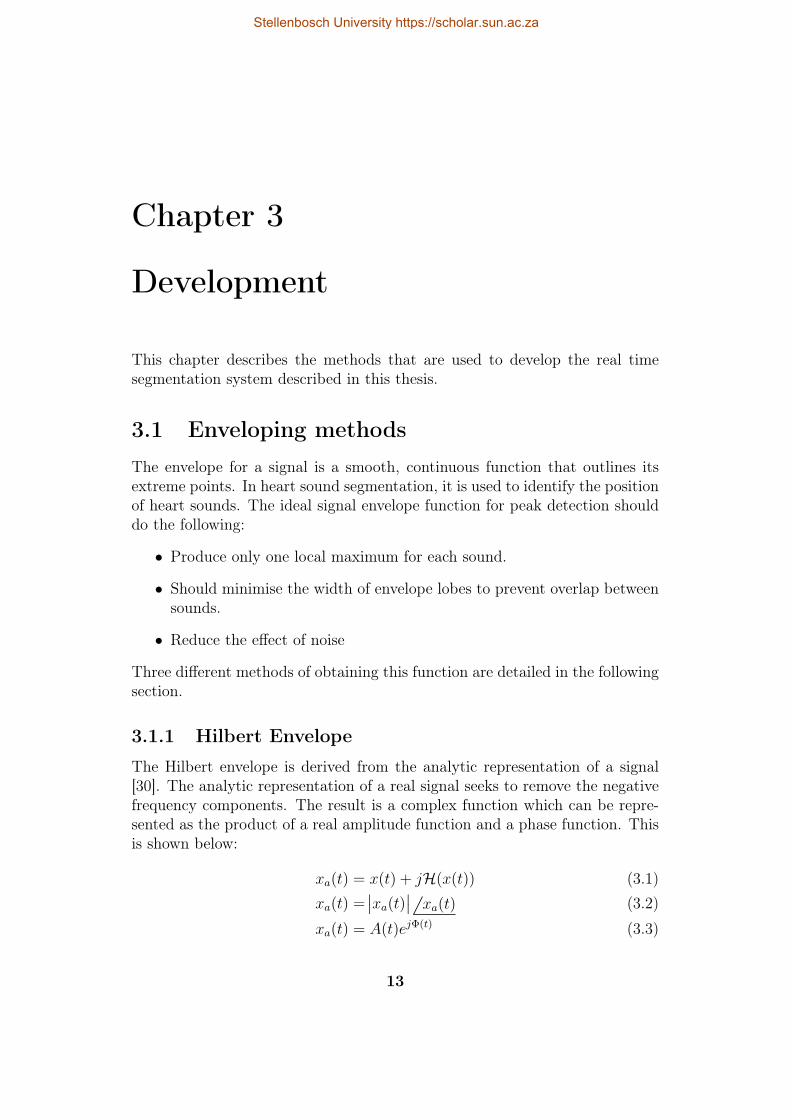
3.1.1 Hilbert Envelope
The Hilbert envelope is derived from the analytic representation of a signal[30]. The analytic representation of a real signal seeks to remove the negativefrequency components. The result is a complex function which can be repre-sented as the product of a real amplitude function and a phase function. Thisis shown below:
xa(t) = x(t) + jH(x(t)) (3.1)xa(t) =
∣∣xa(t)∣∣ xa(t) (3.2)
xa(t) = A(t)ejΦ(t) (3.3)
13
Stellenbosch University https://scholar.sun.ac.za

CHAPTER 3. DEVELOPMENT 14
where x(t) is a real valued signal, xa(t) is the analytic representation of thatsignal, A(t) is the magnitude of the analytic signal and Φ(t) is the phase ofthe analytic signal. An example of a signal and its Hilbert envelope is shownin Figure 3.1.
5.6 5.8 6.0 6.2 6.4 6.6 6.8 7.0
Time (t)
−0.5
0.0
0.5
1.0
Am
plit
ude
PCGHilbert envelope
Figure 3.1: Graph showing the Hilbert envelope of a signal segment
The Hilbert envelope provides the precise definition of a signal envelope.However it does not necessarily produce a single local maximum for a givenheart sound. It is therefore not ideal for finding a local maximum which wouldindicate the position of a heart sound.
3.1.2 Homomorphic Envelope
The homomorphic envelope described in [31] provides a smooth, continuousfunction that tracks the extrema of a signal. It is more impervious to noisefrom murmurs and external sources. The energy of the signal is modelled as themultiplication of two components. A high frequency component, which rep-resents murmurs and noise, and a low frequency component which representsthe components from S1 and S2. To separate the components, the logarithmof the signal amplitude is calculated. This process changes the multiplica-tion of the components into addition, which can be filtered. The frequencycomponents are assumed to remain separable by frequency content after thetransformation. The transformed components are then filtered with a low passfilter to remove the higher frequency component. The resulting signal is thenexponentiated to get the signal envelope. This process is shown below:
x(t) = a(t)f(t) (3.4)log x(t) = log a(t) + log f(t) (3.5)
L(log x(t)) ≈ log a(t) (3.6)
eL(log x(t)) ≈ a(t) (3.7)
Stellenbosch University https://scholar.sun.ac.za

CHAPTER 3. DEVELOPMENT 15
where x(t) is the energy of the signal, a(t) is the low frequency component ofthe energy, f(t) is the high frequency component of the energy and L is theoperator for a low pass filter. The cutoff frequency for the low pass filter Lneeds to be experimentally determined. Figures 3.2,3.3 and 3.4 show the effectof the cutoff frequency of L.
5.6 5.8 6.0 6.2 6.4 6.6 6.8 7.0
Time (t)
−0.5
0.0
0.5
1.0
Am
plit
ude
PCGHomomorphic envelope
Figure 3.2: Graph showing the Homomorphic envelope of a signal segment usinga lowpass filter of 5 Hz
5.6 5.8 6.0 6.2 6.4 6.6 6.8 7.0
Time (t)
−0.5
0.0
0.5
1.0
Am
plit
ude
PCGHomomorphic envelope
Figure 3.3: Graph showing the Homomorphic envelope of a signal segment usinga lowpass filter of 10 Hz
Stellenbosch University https://scholar.sun.ac.za

CHAPTER 3. DEVELOPMENT 16
5.6 5.8 6.0 6.2 6.4 6.6 6.8 7.0
Time (t)
−0.5
0.0
0.5
1.0
Am
plit
ude
PCGHomomorphic envelope
Figure 3.4: Graph showing the Homomorphic envelope of a signal segment usinga lowpass filter of 20 Hz
The Homomorphic envelope produces a more desirable envelope than theHilbert transform. Figure 3.3 only has one local maximum per sound andhas relatively narrow lobes. However it is still sensitive to noise as a localmaximum can be seen in some of the diastolic periods.
3.1.3 Shannon energy envelope
The Shannon energy envelope is derived from the Shannon entropy metric ininformation theory. The reason why the Shannon energy is used is that itperforms as a soft amplitude threshold which emphasises the middle valuesof a normalised signal and de-emphasises loud and soft values. A comparisonwith other types of energy transformation is shown in Figure 3.5. The Shannonenergy envelope is useful for a heart sound signal as the noise is typically soft(background noise) or loud (stethoscope movement). The calculation of theShannon envelope is done by calculating the Shannon energy of the signal thenaveraging it over a fixed period, this is shown below:
xs(t) =1
N
N/2∑i=−N/2
x(t+ i)2 × log∣∣x(t+ i)
∣∣ (3.8)
Stellenbosch University https://scholar.sun.ac.za

CHAPTER 3. DEVELOPMENT 17
0.0 0.2 0.4 0.6 0.8 1.0
Input
0.0
0.2
0.4
0.6
0.8
1.0
Out
put
|x|x2
Shannon EntropyShannon Energy
Figure 3.5: Graph showing the comparison of the different types of energy trans-forms.
The performance of the Shannon energy envelope is dependent on the valuechosen for N. Using a signal with a sampling rate of 1000 Hz, the graphs inFigures 3.6, 3.7 and 3.8 were calculated to show the dependence of N.
5.6 5.8 6.0 6.2 6.4 6.6 6.8 7.0
Time (t)
−0.5
0.0
0.5
1.0
Am
plit
ude
PCGShannon envelope
Figure 3.6: Graph showing the effect of N = 5 on the Shannon Envelope.
5.6 5.8 6.0 6.2 6.4 6.6 6.8 7.0
Time (t)
−0.5
0.0
0.5
1.0
Am
plit
ude
PCGShannon envelope
Figure 3.7: Graph showing the effect of N = 10 on the Shannon Envelope.
Stellenbosch University https://scholar.sun.ac.za

CHAPTER 3. DEVELOPMENT 18
5.6 5.8 6.0 6.2 6.4 6.6 6.8 7.0
Time (t)
−0.5
0.0
0.5
1.0
Am
plit
ude
PCGShannon envelope
Figure 3.8: Graph showing the effect of N = 20 on the Shannon Envelope.
The envelope in Figure 3.8 provides narrow lobes, reduces the effect of theenergy in the diastolic period and minimises the amount of local maxima perheart sound.
3.2 Peak detectionPeak detection is the process of finding all the local maxima in a function.In the analysis of heart sounds, the detection of peaks in the envelope of thesignal is used to identify the location of heart sounds. From calculus, the localmaxima and minima of a function can be found by finding the points wherethe derivative of the function is zero. This formulation works for continuousfunctions, however it does not necessarily work for discrete functions wherethe zero of the derivative could lie between the samples. The solution to thisis to use the change of sign in the derivative. This is equivalent to calculatingthe second derivative. The direction of change is also used to identify the typeof turning point. The process for identifying the local maxima of a signal isshown below:xd[n]← x[n+ 1]− x[n]m← 0for n=0 to N-1 do
if sign(xd[n])=1 and sign(xd[n+ 1])=0 thenp[m]← nm← m+ 1
end ifend for
where x[n] is a discrete function with a lengthN , xd[n] is the discrete equivalentof the derivative of x[n], p is a list containing the locations of the found local
Stellenbosch University https://scholar.sun.ac.za

CHAPTER 3. DEVELOPMENT 19
maxima. The function SIGN is defined as follows:
SIGN(x) =
{1 if x ≥ 0
0 if x < 0
This method accurately identifies all the local maxima in the signal, how-ever there are more local maxima in the signal than there are heart sounds,therefore the list of peaks needs to be filtered to select peaks that are of a largeenough amplitude. The remaining peaks are then processed to resolve peaksthat are within a specific distance of each other.
3.3 Time frequency methodsTime frequency methods are important to the analysis of heart sound signals.This is due to the non stationary nature of heart sounds. They are shortsounds with changing frequency content. These conditions make frequencydomain methods such as Fourier transforms ineffective for analysis. The timefrequency methods that were examined in this thesis are detailed below:
3.3.1 Short Time Fourier transform
The Short Time Fourier Transform (STFT) uses the repeated application ofFourier transform to record the change in the frequency content over time. Itis calculated by taking the Fourier transform of overlapping signal segments.This process is shown below:
STFT(τ, f) =
∫ ∞−∞
x(t)w(t− τ)e−2jπtdt (3.9)
Where τ is the time delay variable, f is the frequency variable, x is the timedomain signal, w is a windowing function. The frequency accuracy of theSTFT is defined by the width of the window function. A narrow windowfunction will yield a transform that localises time accurately, but poorly lo-calises frequency content, conversely, a wide window function yields poor timelocalisation, but good frequency localisation. This concept is explained by theFourier Transform Uncertainty principle [32], which is stated below:(∫ ∞
−∞(t− t0)2
∣∣f(t)∣∣2 dt)(∫ ∞
−∞(ω − ω0)2
∣∣∣f(ω)∣∣∣2 dω) ≥ 1
16π2(3.10)
where f is a normalised, square integrable function and f is the Fourier trans-form of the function. The principle states that the products of the second mo-ments about zero of a normalised, square integrable function and its Fouriertransform has to be greater than or equal to a fixed limit. The second moment
Stellenbosch University https://scholar.sun.ac.za

CHAPTER 3. DEVELOPMENT 20
around zero of the norm of a function is a measure of the dispersal of energy inthe function. The wider the dispersion, the larger the moment. The inequalityonly becomes an equality when f is a normalised Gaussian function. In theSTFT, the dispersion of the function is controlled by the windowing function.Therefore the STFT only performs the analysis at a fixed resolution. This is aproblem as the value of the frequency content changes with the frequency. Forexample, a low frequency sound usually doesn’t need as much time localisationas a high frequency sound.
3.3.2 Wavelet analysis
Wavelet analysis is a generalisation of the Fourier transform which provides amore optimal time-frequency resolution than the STFT. There are two typesof wavelet analysis, there is the Continuous Wavelet Transform(CWT) andthere is the Discrete Wavelet Transform(DWT)
3.3.2.1 Continuous wavelet transform
The CWT is defined as the convolution of the daughter wavelet with theincoming signal. The daughter wavelet provides the optimal time-frequencyfunction for a particular time and frequency.Using the variable names from[24], the wavelet transform of a function f at a time u and scale s is:
Wf (u, s) =
∫ ∞−∞
f(t)Ψ∗u,s(t)dt (3.11)
where Ψu,s(t) is defined as the daughter wavelet of Ψ(t) with the followingrelationship:
Ψu,s(t) =1√s
Ψ
(t− us
)(3.12)
u and s represent the time delay and frequency scale variables.The type of mother wavelet used for analysis is dependent on the appli-
cation. For this thesis, the Morlet wavelet was chosen as it has a high time-frequency resolution [24]. The Morlet wavelet is defined as a time-shiftedgaussian function modulated with a complex exponential. This function isshown below:
Ψ(t) = π−14
(e−jω0t − e−ω2
0/2)e−t
2/2 (3.13)
The value of ω0 is used to change the time-frequency resolution trade off.The affect of ω0 is shown in Figures 3.9 and 3.10. The higher frequency scalingfunctions in 3.10 will have better frequency resolution, but are wider in timeso they will have poorer time resolution. The scaling functions in Figure 3.9have a lower frequency resolution, but have a higher time resolution as theyare narrower. The effect the value of omega on the analysis of heart sounds is
Stellenbosch University https://scholar.sun.ac.za

CHAPTER 3. DEVELOPMENT 21
shown in Figures 3.11 and 3.12. Figure 3.11 has a higher time resolution so isable to resolve time differences between signal components with more accuracy,but does not have sufficient resolution to resolve frequency component data.Figure 3.12 has a higher frequency resolution than 3.11 so more frequencyinformation is visible at a cost of time resolution.
0 2 4 6 8 10 12 14 16
Time (t)
−15
−10
−5
0
5
10
15
Am
plit
ude F = 500.00 Hz
F = 125.00 HzF = 31.25 HzF = 7.81 HzF = 1.95 Hz
Figure 3.9: Graph showing the effect of ω0 = π on scaling functions for differentfrequencies
0 2 4 6 8 10 12 14 16
Time (t)
−6
−4
−2
0
2
4
6
Am
plit
ude
F = 500.00 HzF = 125.00 HzF = 31.25 HzF = 7.81 Hz
Figure 3.10: Graph showing the effect of ω0 = 5π on scaling functions for differentfrequencies
Stellenbosch University https://scholar.sun.ac.za

CHAPTER 3. DEVELOPMENT 22
5.6 5.8 6.0 6.2 6.4 6.6 6.8 7.0
Time (t)
0
50
100
150
200
Fre
quen
cy(H
z)
Figure 3.11: Contour plot showing the effect of ω0 = π on the CWT of heartsounds
5.6 5.8 6.0 6.2 6.4 6.6 6.8 7.0
Time (t)
0
50
100
150
200
Fre
quen
cy(H
z)
Figure 3.12: Contour plot showing the effect of ω0 = 5π on the CWT of heartsounds
3.3.2.2 Discrete wavelet transform
The Discrete Wavelet Transform is an adaption of the CWT to use discretelysampled wavelets. The transform is implemented using a set of discrete filtersarranged in a filter bank with downsampling by two between the levels of thebank. The outputs of the filter banks are the coefficients of the wavelets.The set of filters consists of a bandpass h[n] and a low pass filter g[n]. Thecoefficients from the bandpass filter are called the detail coefficients and thecoefficients from the low pass filter are called the approximation coefficients.This is shown below:
d[n] =∞∑
m=−∞x[m]h[2n−m] (3.14)
a[n] =∞∑
m=−∞x[m]g[2n−m] (3.15)
Stellenbosch University https://scholar.sun.ac.za

CHAPTER 3. DEVELOPMENT 23
where x[n] is the input signal, d[n] are the detail coefficients, a[n] are theapproximation coefficients.
This is shown graphically in Figure 3.3.2.2.
x[n] h[n]
g[n]
2 ↓
2 ↓
d[n]
a[n]
Figure 3.13: Block diagram of one level in a DWT filter bank.
These levels are cascaded to analyse different levels of frequency contentwith each downsampling process halving the level of frequency analysis. Thelow pass filter ensures that the downsampling process does not remove any fre-quencies. The cascaded filterbank with three levels is shown in Figure 3.3.2.2.
x[n] h[n]
g[n]
2 ↓
2 ↓
d1[n]
h[n]
g[n]
2 ↓
2 ↓
d2[n]
h[n]
g[n]
2 ↓
2 ↓
d3[n]
a[n]
Figure 3.14: Block diagram of three levels of a DWT filterbank.
The time-frequency resolution is adjusted by changing the type of wavelet.The Daubechies family of wavelets are commonly used in time/frequency anal-ysis. Figures 3.15 and 3.16 show the differences between the different types ofwavelets on the DWT.
Stellenbosch University https://scholar.sun.ac.za

CHAPTER 3. DEVELOPMENT 24
5.6 5.8 6.0 6.2 6.4 6.6 6.8 7.0
Time (t)
0
100
200
300
400
500
Am
plit
ude
0.00.10.20.30.40.50.60.70.80.91.0
Figure 3.15: 2D heatmap of the distribution of DWT coefficients for the db6wavelet.
5.6 5.8 6.0 6.2 6.4 6.6 6.8 7.0
Time (t)
0
100
200
300
400
500
Am
plit
ude
0.00.10.20.30.40.50.60.70.80.91.0
Figure 3.16: 2D heatmap of the distribution of DWT coefficients for the db3wavelet.
Both of the figures show the change in size of the time-frequency analysiswindows. Figure 3.16 has a higher time resolution than figure 3.15, this allowsfor the shorter, higher frequency components to become visible.
3.3.3 Instantaneous frequency
The frequency component of a signal can be analysed using the analytic rep-resentation of the signal. In analytic signals, the instantaneous frequency ofa signal is represented by the derivative of the phase. The normal way ofcalculating the phase of a signal is to use the arctan function. This becomesproblematic with digital signals as the phase becomes periodic and is bounded
Stellenbosch University https://scholar.sun.ac.za

CHAPTER 3. DEVELOPMENT 25
between −π and π. To get around this problem, the following derivation used.
ω[n] = ρ[n] (3.16)
xa[n] = A[n]ejρ[n] (3.17)ρ[n] = Im[ln(xa[n])] (3.18)
ω[n] = Im[d
dn(ln(xa[n]))] (3.19)
ω[n] = Im[xa[n]
xa[n]] (3.20)
ω[n] ≈ Im[xa[n+ 1]− xa[n]
xa[n]] (3.21)
(3.22)
where ω[n] is the instantaneous frequency and ρ[n] is the phase of x[n]. A fre-quency sweep is shown in Figure 3.17 to demonstrate the ability of the Hilbertinstantaneous frequency to track changes in the signal frequency. The bound-ary effects at the beginning and end are caused by the lack of a windowingfunction in this signal.
0.0 0.5 1.0 1.5 2.0−1.0
−0.5
0.0
0.5
1.0
Am
plit
ude
0.0 0.5 1.0 1.5 2.0
Time (t)
02468
10121416
Fre
quen
cy(H
z)
Figure 3.17: Figure showing a frequency sweep from 5 Hz to 15 Hz
The instantaneous frequency of a signal segment from a heart sound isshown in Figure 3.18. The high frequency noise in the signal makes this typeof analysis difficult.
Stellenbosch University https://scholar.sun.ac.za

CHAPTER 3. DEVELOPMENT 26
5.4 5.6 5.8 6.0 6.2 6.4 6.6 6.8 7.0
Time (t)
0
200
400
600
800
1000
1200
1400
Fre
quen
cy(H
z)
Figure 3.18: Plot showing the instantaneous frequency content of heart sounds
3.4 Statistical clusteringK-means clustering is a statistical method of grouping together a set of vectorsinto a specified k number of clusters [33]. Each cluster is associated with amean that determines how the date points are assigned to each cluster. Thealgorithm iterates over the following steps until the assignment of vectors doesnot change between iterations.
Assignment Each vector is assigned a cluster based on minimising the Eu-clidean distance from each particular vector to the centroid of the cluster.
Update New centroids calculate by finding the mean of all the vectors as-signed to a particular cluster,
3.5 SummaryThis section introduced the various signal processing and statistical techniquesof analysis used in this thesis.
Stellenbosch University https://scholar.sun.ac.za

Chapter 4
Method
This chapter introduces the segmentation method and testing procedure usedin this thesis.
4.1 Inspiration for methodThe coefficients from a continuous wavelet transform contain sufficient infor-mation to identify S1 from S2 [24]. The current technology utilises machinelearning to separate the heart sounds with these coefficients. This method doesnot take advantage of the inherent repetition of the different heart sounds. Totake advantage of this property, correlation is used, specifically the correlationof the continuous wavelet transform coefficients. The CWT was used over theDWT as the system was implemented on a desktop computer which could cal-culate the higher resolution CWT of a heart sound sufficiently quickly for realtime processing.
4.2 AlgorithmThere are two algorithms that this thesis introduces. An algorithm that seg-ments pre-recorded sounds and an algorithm that segments sounds that arenot pre-recorded.
4.2.1 Offline sound segment identification
The following assumptions are made about the sounds that are emanate fromthe heart:
• The time-frequency content for S1 and S2 cover similar regions in thedomain
• The time frequency content for S1 is different than that of S2
27
Stellenbosch University https://scholar.sun.ac.za

CHAPTER 4. METHOD 28
• The selectional regional correlation of one sound with another yields amaximum when the two sounds are similar.
Record sig-nal segment
Heart sound loca-tion identification
Time frequencydata extraction
Time frequencytransformation
Selectional regionalcorrelation as afeature vector
Clustering theheart sounds
Identificationof clusteredheart sounds
Figure 4.1: Flow diagram showing the layout of the S1 - S2 detection system
4.2.1.1 Heart sound location identification
To identify the origins of all the sounds in a signal, the location of each soundis required. This is achieved by identifying the peaks in the Shannon envelopeof the signal. The Shannon envelope of a heart sound segment is shown inFigure 4.2.
4.5 5.0 5.5 6.0 6.5 7.0 7.5 8.0 8.5
Time (t)
−0.5
0.0
0.5
1.0
Am
plit
ude
S1S1 S1
S1 S1S2
S2
S2 S2
S2
PCGShannon energyPeaks
Figure 4.2: Graph showing the Envelope, PCG and identified peaks.
4.2.1.2 Time frequency data extraction
The CWT for each sound is calculated from a segment of signal around eachlocated peak. The segment length is calculated from the width of the peaksin the Shannon envelope. The magnitude of the CWT of the signal in Figure4.2 is shown in Figure 4.3.
Stellenbosch University https://scholar.sun.ac.za
CHAPTER 4. METHOD 29
4.5 5.0 5.5 6.0 6.5 7.0 7.5 8.0 8.5
Time (t)
50
100
150
200
Fre
quen
cy(H
z)
Figure 4.3: Graph showing wavelet coefficients of the signal.
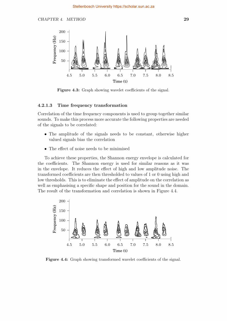
4.2.1.3 Time frequency transformation
Correlation of the time frequency components is used to group together similarsounds. To make this process more accurate the following properties are neededof the signals to be correlated:
• The amplitude of the signals needs to be constant, otherwise highervalued signals bias the correlation
• The effect of noise needs to be minimised
To achieve these properties, the Shannon energy envelope is calculated forthe coefficients. The Shannon energy is used for similar reasons as it wasin the envelope. It reduces the effect of high and low amplitude noise. Thetransformed coefficients are then thresholded to values of 1 or 0 using high andlow thresholds. This is to eliminate the effect of amplitude on the correlation aswell as emphasising a specific shape and position for the sound in the domain.The result of the transformation and correlation is shown in Figure 4.4.
4.5 5.0 5.5 6.0 6.5 7.0 7.5 8.0 8.5
Time (t)
50
100
150
200
Fre
quen
cy(H
z)
Figure 4.4: Graph showing transformed wavelet coefficients of the signal.
Stellenbosch University https://scholar.sun.ac.za

CHAPTER 4. METHOD 30
4.2.1.4 Selectional regional correlation as a feature vector
To segment the located sounds, the selectional regional correlation for eachsound is calculated with respect to all the other sounds in the signal. Thetime frequency correlation for two sounds is calculated by multiplying thecomponents of the two sounds together and summing the result. The correla-tion for a particular sound is expected to increase when the compared sound issimilar and decrease when the sound is dissimilar. The patterns of increasingand decreasing levels of similarity are shown in Figure 4.5.
4.5 5.0 5.5 6.0 6.5 7.0 7.5 8.0 8.5
Time (t)
−3
−2
−1
0
1
2
3
4
Cor
rela
tion
sim
ilari
ty
Figure 4.5: Graph showing the correlation of the transformed wavelet coefficients.
4.2.1.5 Clustering the heart sounds
The selectional regional correlation for a particular sound is used as a featurevector for a machine learning system. Each dimension in the vector representshow similar the sound is with another sound. The heart sounds are thenclustered using the k-means clustering algorithm. The clustered correlationsare shown in Figure 4.6.
4.5 5.0 5.5 6.0 6.5 7.0 7.5 8.0 8.5
Time (t)
−3
−2
−1
0
1
2
3
4
Cor
rela
tion
sim
ilari
ty
Figure 4.6: Graph showing the grouped correlations of the signal.
Stellenbosch University https://scholar.sun.ac.za

CHAPTER 4. METHOD 31
4.2.1.6 Identification of clustered heart sounds
The clustered correlations are then used to separate the heart sounds intotwo groups. These groups will each contain a number of sounds that aresimilar to each other. The next step is to identify the source of each group ofsimilar sounds. The time difference between successive S1 and S2 sounds issmaller than time difference between successive S2 and S1 sounds. Using thisinformation, the groups are identified as either S1 or S2 based on the averagetransaction time between the identified groups. Whilst this method is similarto the method in 2.4.1.1, the comparison is made between groups of similarlysounding heart sounds as opposed to ungrouped sounds.
4.2.2 Online segmentation
The algorithm in section 4.2.1 is adapted to real time usage by using a templateof identified sounds, which is generated during a short setup stage of a fewseconds, to group an identified sound instead of using k-means. An overviewof the methods is shown in Figure 4.7.
Model creation(per section 4.2.1)
Identify loca-tion of sound
Calculate timefrequency contentof located sounds
Calculate thecorrelation of thelocated sounds
Identificationof sounds
Validation ofidentified sounds
Figure 4.7: Flow diagram showing the layout of the real time system
4.2.2.1 Model creation
To identify a heart sound in real time, the system first needs to generate tem-plates of S1 and S2 sounds with which an unknown sound can be correlated.The templates are constructed from the transformed time frequency coeffi-cients of identified S1 and S2 an initial recording (5 seconds minimum). Thetemplates are arranged in an alternating pattern of groups, namely S1 and S2.With the templates in a pattern, the correlation of the templates is calculatedand the mean value of the correlation in each group is found. This is theequivalent of performing the k-means algorithm on the correlations.
4.2.2.2 Identify location of sound
The real time analysis of the signal is performed on overlapping 2 secondchunks of data with a refresh rate of 1 second. These intervals guarantee thatat least one sound is captured in the chunk as the average heart rate is 60 to100 beats per minute. In each 2 second chunk of data, the Shannon envelope
Stellenbosch University https://scholar.sun.ac.za

CHAPTER 4. METHOD 32
is calculated and the peaks are found. The peaks represent the location of apotential heart sound.
4.2.2.3 Calculate time frequency content of located sounds
The time frequency content of each identified sound is calculated and trans-formed in the same way as subsections 4.2.1.2 through 4.2.1.3.
4.2.2.4 Calculate correlation of identified sounds
The identified sounds are correlated with the S1-S2 template to generate fea-ture vectors to identify the sounds.
4.2.2.5 Identification of sounds
The sounds are identified by calculating the Euclidean distance from theirfeature vectors to each of the means calculated in section 4.2.2.1. The groupwith the smallest distance is chosen as the label for the sound being identified.
4.2.2.6 Validation of identified sounds
To increase the accuracy of the system, a simple method of validation is used.The method consists of only using pairs of sounds that correspond to thephysiological process. Therefore the only sound pairs that are used are the S1to S2 pair and the S2 to S1 pair. Any other pair is considered to be an errorin identification.
4.3 Synthetic testbedThe testing of any algorithm is essential to determine its effectiveness, specif-ically testing how an algorithm copes with a low signal to noise ratio. Thistype of testing is difficult for a heart sound segmentation algorithm as thesignals are inherently noisy and do not have established models for the dif-ferent sounds. There are also problems concerning the type of noise in thesignal. There is firstly uncorrelated white noise which would represent back-ground noise from the body and recording environment. This type of noise isrelatively easy to test with, as it involves adding generated white noise to asignal that is considered noise free then adjusting the amplitude of the noiseto obtain the desired signal to noise ratio. The other type of noise that isassociated with heart sounds is the correlated noise that arises from murmursand S3 and S4 heart sounds. This type of noise is more problematic for asegmentation algorithm as well as being more difficult to test. This sectionshows the development of a synthetic testing platform using a sum of fittedGaussian modulated sinusoidal functions.
Stellenbosch University https://scholar.sun.ac.za

CHAPTER 4. METHOD 33
4.3.1 Signal synthesis
The synthetic heart sounds are generated from a previously segmented heartsound signal. For each detected heart sound in the signal, a sum of gaussiansinusoids is fitted to the sound using the following algorithm:
• Set initial parameters to a low frequency
• Use least squares fitting to change the parameters of the function tominimise the error between the original function and the fitted function
• Subtract the fitted function from the original function, increase the initialfrequency and repeat.
The Gaussian modulated function and its parameters are shown below:
G(t, A, f0, σ, t0, φ) = A cos(2πf0(t− t0)− φ)e−(t−t0σ
)2 (4.1)
The process is shown in Figures 4.8,4.9,4.10 and 4.11.
5.4 5.6 5.8 6.0 6.2 6.4 6.6 6.8 7.0
Time (t)
−1.0−0.8−0.6−0.4−0.2
0.00.20.40.60.8
Am
plit
ude
5.4 5.6 5.8 6.0 6.2 6.4 6.6 6.8 7.0
Time (t)
−1.0−0.8−0.6−0.4−0.2
0.00.20.40.60.8
Am
plit
ude
Figure 4.8: Graphs showing the original signal and the first approximation.
Stellenbosch University https://scholar.sun.ac.za

CHAPTER 4. METHOD 34
5.4 5.6 5.8 6.0 6.2 6.4 6.6 6.8 7.0
Time (t)
−1.0−0.8−0.6−0.4−0.2
0.00.20.40.60.8
Am
plit
ude
5.4 5.6 5.8 6.0 6.2 6.4 6.6 6.8 7.0
Time (t)
−1.0−0.8−0.6−0.4−0.2
0.00.20.40.60.8
Am
plit
ude
Figure 4.9: Graphs showing the original signal and the second approximation.
5.4 5.6 5.8 6.0 6.2 6.4 6.6 6.8 7.0
Time (t)
−1.0−0.8−0.6−0.4−0.2
0.00.20.40.60.8
Am
plit
ude
5.4 5.6 5.8 6.0 6.2 6.4 6.6 6.8 7.0
Time (t)
−1.0−0.8−0.6−0.4−0.2
0.00.20.40.60.8
Am
plit
ude
Figure 4.10: Graphs showing the original signal and the third approximation.
Stellenbosch University https://scholar.sun.ac.za

CHAPTER 4. METHOD 35
5.4 5.6 5.8 6.0 6.2 6.4 6.6 6.8 7.0
Time (t)
−1.0−0.8−0.6−0.4−0.2
0.00.20.40.60.8
Am
plit
ude
5.4 5.6 5.8 6.0 6.2 6.4 6.6 6.8 7.0
Time (t)
−1.0−0.8−0.6−0.4−0.2
0.00.20.40.60.8
Am
plit
ude
Figure 4.11: Graphs showing the original signal and the final approximation.
The parameters for each level of approximation in each heart sound areused to build a random distribution from which new parameters can be drawnfrom. This is done to approximate the random nature of biological signals.
4.3.2 Signal generation
The test signals are generated by drawing the parameters for the Gaussianfunctions from the random distributions. The process for generating the signalsstarts with determining the positions of the heart sounds based on the heartrate. Once the positions are calculated a heart sound is generated for thatposition by using the values from the random distribution. To ensure that heartsounds in their respective groups have a degree of similarity, the distributionsfor the two approximations with the highest energy are modified to have alower standard deviation. These two approximations are then treated as thepart of the signal which contains the information required for segmentation.The rest of the approximations are treated as additive noise. Gaussian whitenoise is then added to the signal to simulate background noise from the body.Three different generated signals for different heart rates are shown in Figures4.12, 4.13 and 4.14.
Stellenbosch University https://scholar.sun.ac.za
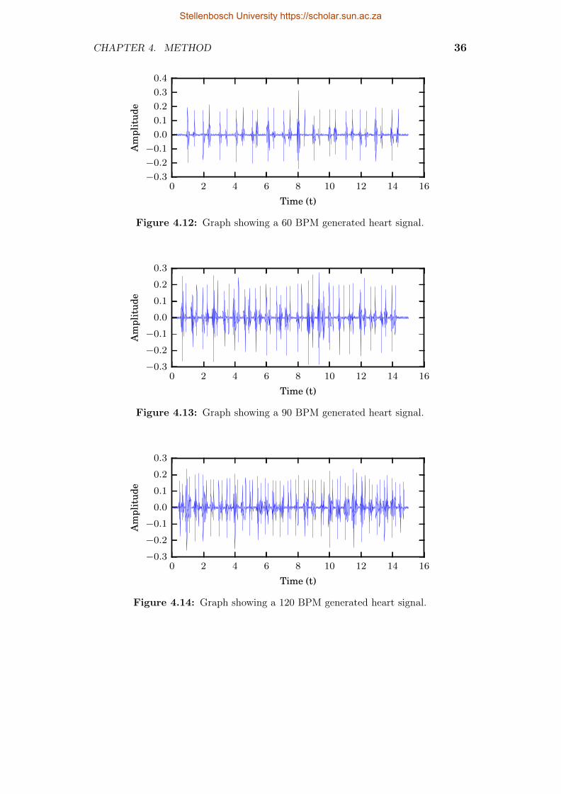
CHAPTER 4. METHOD 36
0 2 4 6 8 10 12 14 16
Time (t)
−0.3
−0.2
−0.1
0.0
0.1
0.2
0.3
0.4
Am
plit
ude
Figure 4.12: Graph showing a 60 BPM generated heart signal.
0 2 4 6 8 10 12 14 16
Time (t)
−0.3
−0.2
−0.1
0.0
0.1
0.2
0.3
Am
plit
ude
Figure 4.13: Graph showing a 90 BPM generated heart signal.
0 2 4 6 8 10 12 14 16
Time (t)
−0.3
−0.2
−0.1
0.0
0.1
0.2
0.3
Am
plit
ude
Figure 4.14: Graph showing a 120 BPM generated heart signal.
Stellenbosch University https://scholar.sun.ac.za

CHAPTER 4. METHOD 37
4.4 SummaryThis chapter introduced a heart sound segmentation method that can detectthe first and second heart sounds in real time. It also introduced a method forgenerating heart sound signals with a controllable signal to noise ratio.
Stellenbosch University https://scholar.sun.ac.za

Chapter 5
Testing
This chapter documents the testing done on the algorithms developed in chap-ter 4. The three types of testing done in this chapter are offline, synthetic andonline testing.
5.1 Offline testingThis section documents the testing of the system using prerecorded heartsounds from test subjects. The sounds were recorded at the Red Cross chil-dren’s hospital under ethical conditions. The dataset was captured from thefour areas of auscultation in 230 healthy subjects.The signals were recorded at22 kHz and were each 15 seconds long. The prerecorded signals were manuallysegmented with the assistance of an ECG and the results saved in a database.Each of the signals were segmented using the offline method described in sec-tion 4.2.1.
5.1.1 Offline testing results
The results of segmentation are shown in Table 5.1:
Manuallyidentified S1
Manuallyidentified S2
Manually identifiedother
Systemidentified S1 2444 508 15
Systemidentified S2 334 2168 18
Table 5.1: Table to show results of the system implemented in this thesis.
38
Stellenbosch University https://scholar.sun.ac.za

CHAPTER 5. TESTING 39
5.1.2 Offline testing evaluation
The two measures used to evaluate the performance of the algorithm are theheart sound hit rate and the heart sound accuracy. The heart sound hit raterefers to the amount of sounds correctly identified out of the total number ofsounds of that type in the signal. The hit rate gives a measure of how sensitivethe system is to detecting a heart sound in a signal. For these results, the hitrate is:
S1HR =2444
2444 + 334= 87.9% (5.1)
S2HR =2168
2168 + 508= 81.0% (5.2)
The heart sound accuracy rate refers to the amount of sounds that werecorrect out of the sounds that were identified. This gives a measure of howmuch the system’s results can be trusted. For these results, the accuracy rateis:
S1AR =2444
2444 + 508 + 15= 82.3% (5.3)
S2AR =2168
2168 + 508 + 18= 86.1% (5.4)
(5.5)
The average implementation time on a dual core i5 laptop is broken downbelow:
CWT calculation : 0.09 seconds
CWT correlation : 0.038 seconds
Feature vector calculation : 0.0128 seconds
k-means : 0.0003 seconds
Total : 1.36 seconds
5.1.3 Offline testing discussion
The evaluation of the algorithm shows the system is capable of accuratelydetecting the majority of heart sounds in the database with an average hitrate of 84.4% and an average accuracy rate of 84.2%. These performancerates prove that the algorithm in this thesis is capable of segmenting heartsounds reasonably accurately. When testing the performance of segmentationalgorithms, it is difficult to construct a fair test that accurately simulates realworld performance. The difficulty comes from the source of the testing data asthere is no control over the conditions that generate the data, other than the
Stellenbosch University https://scholar.sun.ac.za
CHAPTER 5. TESTING 40
selection of the data itself. The dataset used in this testing for example couldcontain 15 % of fundamentally unusable sounds, if this was the case, having ahit rate of near 85 % would actually mean the algorithm is working very well.The problem is it is impossible to objectively obtain the unusable sounds. Oneway to reduce the effect of this is to apply some selection criteria to the signal,such as a visual threshold. This would increase the apparent performanceof the algorithm as there would be less undetectable sound. This processmight lead to incorrect conclusions about the performance of the algorithmas the data are cherry picked. On the other hand, no algorithm is capableof producing results from data that for all intents and purposes is junk, soincluding it would unfairly decrease the apparent performance as well. Theonly real to get around this problem is to use a large set of data to test thealgorithm on and hope that there is an equal distribution of “perfect” signalsand junk signals. This method has its problems as well as to manually verifysuch a large dataset is unfeasible. This is what motivated the use of synthetictesting.
The implementation time break down indicates that the calculation time forthe feature vector is fast enough to be implemented in real time as the distancebetween subsequent heart sounds is significantly more than 12 milliseconds.
5.2 Synthetic testingThe testing in Section 5.1 only shows how the system performs against realsignals with little control on the quality. To test the segmentation ability ofthe algorithm in controlled, noisy environments, the generated signals with aknown signal to noise ratio from Section 4.3.1 are used. To set the signal tonoise ratio, a synthetic signal is generated with separate noise and heart signalcomponents. The SNR for this signal is calculated and used to calculate aconstant multiple for the heart signal which will set the SNR to the desiredlevel. This calculation is shown below:
SNRold = 10× log
(∑Ni=0 xs[i]
2∑Ni=0 xn[i]2
)(5.6)
c = 10
(SNRdes−SNRold
20
)(5.7)
xs[i] = c× xs[i] (5.8)
where SNRold is the signal to noise ratio of the generated signal, xs is theheart signal component, xn is the noise signal component and SNRdes is thedesired signal to noise ratio. Two types of noise are tested in this section, cor-related noise and uncorrelated noise. Correlated noise refers to the additionalGaussian modulated components that are drawn from a random distribution.Uncorrelated noise refers to Gaussian white noise. The testing in this sec-tion tests the algorithm against both types individually and in combination.
Stellenbosch University https://scholar.sun.ac.za

CHAPTER 5. TESTING 41
The testing procedure test the algorithm against a range of signals with dif-ferent SNRs. At each chosen level of SNR, 50 different signals are generated,segmented and evaluated, with the metrics from Subsectionsect:eval used toevaluate the performance. Twenty different levels equally spaced were chosenbetween -200dB and 5 dB, yielding a total of 2000 different sounds tested foreach heart rate. Three different heart rates were tested.
5.2.1 Synthetic testing interpetation
The graphs in Subsections 5.2.2, 5.2.3 and 5.2.4 show that noise starts hinder-ing the accuracy at -10dB and the hit rate at -10dB, regardless of the type ofnoise added. The graphs also indicate that the sensitivity to noise increaseswith the heart rate, also regardless of the type of noise added. The graphsshow the type of noise that has the most effect on the segmentation ability isuncorrelated noise, whilst correlated noise has the least effect. The additionof correlated noise to uncorrelated noise did not present a significant changeto the segmentation ability of the system.
The synthetic testing provides insight into where this algorithm will beuseful. The robustness against the correlated noise means that the algorithm isrobust against the time-frequency variation that occurs between heart sounds.The sensitivity to uncorrelated noise does not affect the effectiveness of thealgorithm as this type of noise is easy for a health care provider to identifyand correct.
5.2.2 Uncorrelated noise testing results
Four examples of a generated signal with this type of noise at different levelsare provided in Figures 5.1, 5.2 and5.3
0 2 4 6 8 10 12 14 16
Time (t)
−0.015
−0.010
−0.005
0.000
0.005
0.010
Am
plit
ude
Figure 5.1: Graph showing a generated signal with uncorrelated noise with a SNRof -50dB.
Stellenbosch University https://scholar.sun.ac.za

CHAPTER 5. TESTING 42
0 2 4 6 8 10 12 14 16
Time (t)
−0.015
−0.010
−0.005
0.000
0.005
0.010
Am
plit
ude
Figure 5.2: Graph showing a generated signal with uncorrelated noise with a SNRof -15dB.
0 2 4 6 8 10 12 14 16
Time (t)
−0.03
−0.02
−0.01
0.00
0.01
0.02
0.03
Am
plit
ude
Figure 5.3: Graph showing a generated signal with uncorrelated noise with a SNRof 5dB.
The results for the testing at three different heart rates are shown in Figures5.4, 5.5, and 5.6.
Stellenbosch University https://scholar.sun.ac.za
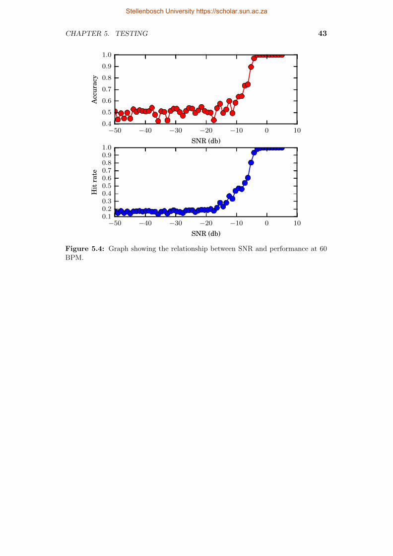
CHAPTER 5. TESTING 43
−50 −40 −30 −20 −10 0 10
SNR (db)
0.4
0.5
0.6
0.7
0.8
0.9
1.0
Acc
urac
y
−50 −40 −30 −20 −10 0 10
SNR (db)
0.10.20.30.40.50.60.70.80.91.0
Hit
rate
Figure 5.4: Graph showing the relationship between SNR and performance at 60BPM.
Stellenbosch University https://scholar.sun.ac.za

CHAPTER 5. TESTING 44
−50 −40 −30 −20 −10 0 10
SNR (db)
0.4
0.5
0.6
0.7
0.8
0.9
1.0
Acc
urac
y
−50 −40 −30 −20 −10 0 10
SNR (db)
0.10.20.30.40.50.60.70.80.91.0
Hit
rate
Figure 5.5: Graph showing the relationship between SNR and performance at 90BPM
Stellenbosch University https://scholar.sun.ac.za

CHAPTER 5. TESTING 45
−50 −40 −30 −20 −10 0 10
SNR (db)
0.4
0.5
0.6
0.7
0.8
0.9
1.0
Acc
urac
y
−50 −40 −30 −20 −10 0 10
SNR (db)
0.10.20.30.40.50.60.70.80.91.0
Hit
rate
Figure 5.6: Graph showing the relationship between SNR and performance at 120BPM.
5.2.3 Correlated noise testing results
Four examples of signals with different levels of correlated noise are shown inFigures, 5.7, 5.8 and 5.9.
0 2 4 6 8 10 12 14 16
Time (t)
−0.15
−0.10
−0.05
0.00
0.05
0.10
0.15
0.20
Am
plit
ude
Figure 5.7: Graph showing a generated signal with correlated noise with a SNR of-50dB.
Stellenbosch University https://scholar.sun.ac.za
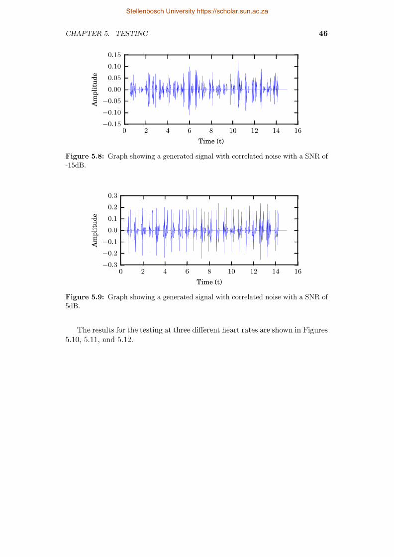
CHAPTER 5. TESTING 46
0 2 4 6 8 10 12 14 16
Time (t)
−0.15
−0.10
−0.05
0.00
0.05
0.10
0.15
Am
plit
ude
Figure 5.8: Graph showing a generated signal with correlated noise with a SNR of-15dB.
0 2 4 6 8 10 12 14 16
Time (t)
−0.3
−0.2
−0.1
0.0
0.1
0.2
0.3
Am
plit
ude
Figure 5.9: Graph showing a generated signal with correlated noise with a SNR of5dB.
The results for the testing at three different heart rates are shown in Figures5.10, 5.11, and 5.12.
Stellenbosch University https://scholar.sun.ac.za

CHAPTER 5. TESTING 47
−50 −40 −30 −20 −10 0 10
SNR (db)
0.60
0.65
0.70
0.75
0.80
0.85
0.90
0.95
1.00
Acc
urac
y
−50 −40 −30 −20 −10 0 10
SNR (db)
0.2
0.3
0.4
0.5
0.6
0.7
0.8
0.9
1.0
Hit
rate
Figure 5.10: Graph showing the relationship between SNR and performance at 60BPM.
Stellenbosch University https://scholar.sun.ac.za
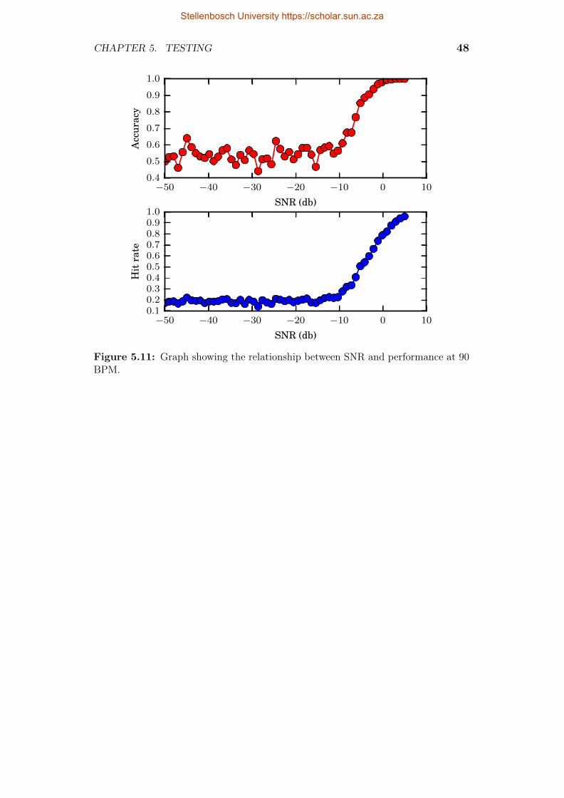
CHAPTER 5. TESTING 48
−50 −40 −30 −20 −10 0 10
SNR (db)
0.4
0.5
0.6
0.7
0.8
0.9
1.0
Acc
urac
y
−50 −40 −30 −20 −10 0 10
SNR (db)
0.10.20.30.40.50.60.70.80.91.0
Hit
rate
Figure 5.11: Graph showing the relationship between SNR and performance at 90BPM.
Stellenbosch University https://scholar.sun.ac.za

CHAPTER 5. TESTING 49
−50 −40 −30 −20 −10 0 10
SNR (db)
0.3
0.4
0.5
0.6
0.7
0.8
0.9
1.0
Acc
urac
y
−50 −40 −30 −20 −10 0 10
SNR (db)
0.00.10.20.30.40.50.60.70.80.9
Hit
rate
Figure 5.12: Graph showing the relationship between SNR and performance at 120BPM.
5.2.4 Correlated and uncorrelated noise testing results
Four examples of signals with correlated and white noise are provided in Fig-ures 5.13, 5.14 and 5.15
0 2 4 6 8 10 12 14 16
Time (t)
−0.15
−0.10
−0.05
0.00
0.05
0.10
0.15
Am
plit
ude
Figure 5.13: Graph showing a generated signal with correlated noise with a SNRof -50dB.
Stellenbosch University https://scholar.sun.ac.za

CHAPTER 5. TESTING 50
0 2 4 6 8 10 12 14 16
Time (t)
−0.15
−0.10
−0.05
0.00
0.05
0.10
0.15
Am
plit
ude
Figure 5.14: Graph showing a generated signal with correlated noise with a SNRof -15dB.
0 2 4 6 8 10 12 14 16
Time (t)
−0.3
−0.2
−0.1
0.0
0.1
0.2
0.3
Am
plit
ude
Figure 5.15: Graph showing a generated signal with correlated noise with a SNRof 5dB.
The results for the testing at three different heart rates are shown in Figures5.4, 5.5, and 5.6.
Stellenbosch University https://scholar.sun.ac.za

CHAPTER 5. TESTING 51
−50 −40 −30 −20 −10 0 10
SNR (db)
0.60
0.65
0.70
0.75
0.80
0.85
0.90
0.95
1.00
Acc
urac
y
−50 −40 −30 −20 −10 0 10
SNR (db)
0.2
0.3
0.4
0.5
0.6
0.7
0.8
0.9
1.0
Hit
rate
Figure 5.16: Graph showing the relationship between SNR and performance at 60BPM.
Stellenbosch University https://scholar.sun.ac.za

CHAPTER 5. TESTING 52
−50 −40 −30 −20 −10 0 10
SNR (db)
0.4
0.5
0.6
0.7
0.8
0.9
1.0
Acc
urac
y
−50 −40 −30 −20 −10 0 10
SNR (db)
0.10.20.30.40.50.60.70.80.91.0
Hit
rate
Figure 5.17: Graph showing the relationship between SNR and performance at 90BPM.
Stellenbosch University https://scholar.sun.ac.za

CHAPTER 5. TESTING 53
−50 −40 −30 −20 −10 0 10
SNR (db)
0.3
0.4
0.5
0.6
0.7
0.8
0.9
1.0
Acc
urac
y
−50 −40 −30 −20 −10 0 10
SNR (db)
0.00.10.20.30.40.50.60.70.80.9
Hit
rate
Figure 5.18: Graph showing the relationship between SNR and performance at 120BPM.
5.3 Online testingThe functionality of the real time system was tested by monitoring the heartsounds of the author. The screen capture of the process in shows how thesystem is capable of segmentation in real time. The video can be viewed onthe link in [34]. The video shows 60 seconds of real time analysis in which39 pairs of S1 and S2 sounds are observed. Out of these 39 pairs, 24 wereidentified as S1-S2 pairs, with no incorrect sounds reported. This preliminarytest shows the system is capable of identifying heart sounds in real time.
5.4 SummaryThis section shows that the algorithm described in this thesis is capable of ac-curate heart sound segmentation of real signals, both in an online and offlinecapability. The algorithm is robust to different types of noise as the perfor-mance of the algorithm is more dependent on the amount of noise than thetype. This makes it suitable for “real world” conditions where murmurs arepresent.
Stellenbosch University https://scholar.sun.ac.za

Chapter 6
Conclusion
From the examination of the literature, it was postulated that it was possibleto identify a heart sound from other heart sounds based on its time-frequencycontent, which would satisfy Hypothesis 1.1 as time frequency content is shortin length. The development and subsequent testing of the offline algorithmshowed that the time frequency content of individual heart sounds, when trans-formed and correlated provides a feature vector that can separate the differenttypes of heart sounds. An average accuracy of 84.2 % and a hit rate of 84.4% indicate that the algorithm is a suitable candidate for further development.The algorithm in this thesis was tested against synthetic heart sounds thathave a known signal to noise ratio. This allowed for the determination ofwhere the algorithm will start to fail. The upper bound for where the algo-rithm will start to fail is -10dB of noise for the three heart rates tested in thisthesis. The two offline testing results prove Hypothesis 1.1 and 1.2.
The real time segmentation of the heart sounds was tested on a singlesubject and was found to work flawlessly in detecting S1 and S2. This resultand the short feature vector calculation time show prove Hypothesis 2.1.
Future work should be aimed at exploring the different types of time fre-quency analysis methods and testing them with the procedures in this thesis,along with other segmentation algorithms. The integration of existing methodsof analysing segmented sounds is also a potential candidate for future work.Given the financial constraints of the expected operating environment, an ef-ficient mobile implementation of the algorithm should also be investigated foruse in telemedicine.
54
Stellenbosch University https://scholar.sun.ac.za

Bibliography
[1] Nannan, N., Dorrington, R., Laubscher, R., Zinyakatira, N., Prinsloo, M.,Darikwa, T., Matzopoulos, R. and Bradshaw, D.: Under-5 mortality statisticsin south africa. 2012.
[2] Martini, F.H., Bartholomew, E.F., Ober, W.C., Garrison, C.W., Welch, K. andHutchings, R.: Essentials of anatomy & physiology. Pearson, 2003.
[3] Hoffman, J.I. and Kaplan, S.: The incidence of congenital heart disease. Journalof the American College of Cardiology, vol. 39, no. 12, pp. 1890–1900, 2002.
[4] Shub, C.: Echocardiography or auscultation? how to evaluate systolic murmurs.Canadian family physician, vol. 49, no. 2, pp. 163–167, 2003.
[5] Thompson, W., Hayek, C., Tuchinda, C., Telford, J. and Lombardo, J.: Auto-mated cardiac auscultation for detection of pathologic heart murmurs. Pediatriccardiology, vol. 22, no. 5, pp. 373–379, 2001.
[6] Geggel, R.L., Horowitz, L.M., Brown, E.A., Parsons, M., Wang, P.S. and Ful-ton, D.R.: Parental anxiety associated with referral of a child to a pediatriccardiologist for evaluation of a still’s murmur. The Journal of pediatrics, vol.140, no. 6, pp. 747–752, 2002.
[7] Watrous, R.L., Thompson, W.R. and Ackerman, S.J.: The impact of computer-assisted auscultation on physician referrals of asymptomatic patients with heartmurmurs. Clinical cardiology, vol. 31, no. 2, pp. 79–83, February 2008. ISSN0160-9289.Available at: http://www.ncbi.nlm.nih.gov/pubmed/18257026
[8] Zimetbaum, P. and Goldman, A.: Ambulatory arrhythmia monitoring choosingthe right device. Circulation, vol. 122, no. 16, pp. 1629–1636, 2010.
[9] Coovadia, H., Jewkes, R., Barron, P., Sanders, D. and McIntyre, D.: The healthand health system of south africa: historical roots of current public healthchallenges. The Lancet, vol. 374, no. 9692, pp. 817–834, 2009.
[10] Hoosen, E.G.M., Cilliers, A.M., Hugo-Hamman, C.T., Brown, S.C., Lawrenson,J.B., Zuhlke, L. and Hewitson, J.: Paediatric cardiac services in South Africa.SAMJ: South African Medical Journal, , no. 2, p. 106. ISSN 0256-9574.
55
Stellenbosch University https://scholar.sun.ac.za
BIBLIOGRAPHY 56
[11] Hanna, I.R. and Silverman, M.E.: A history of cardiac auscultation and some ofits contributors. The American journal of cardiology, vol. 90, no. 3, pp. 259–267,2002.
[12] Felner, J.M.: The First Heart Sound. In: Walker, H., WD, H. and JW, H.(eds.), Clinical Methods: The History, Physical, and Laboratory Examinations.,3rd edn, chap. 22. Butterworths, 1990.
[13] Alam, U., Asghar, O., Malik, R.A., Khan, S. and Hayat, S.: Cardiac ausculta-tion: an essential clinical skill in decline. The British Journal of Cardiology, ,no. 1, pp. –10.
[14] Dice, J.E. and Bhatia, J.: Patent ductus arteriosus: an overview. The Journalof Pediatric Pharmacology and Therapeutics, vol. 12, no. 3, pp. 138–146, 2007.
[15] Pretorius, E., Cronje, M.L. and Strydom, O.: Development of a pediatric cardiaccomputer aided auscultation decision support system. Conference proceedings :... Annual International Conference of the IEEE Engineering in Medicine andBiology Society. IEEE Engineering in Medicine and Biology Society. AnnualConference, vol. 2010, pp. 6078–82, January 2010. ISSN 1557-170X.Available at: http://www.ncbi.nlm.nih.gov/pubmed/21097128
[16] Felner, J.M.: The Second Heart Sound. In: Walker, H., Hall WD and Hurst JW(eds.), Clinical Methods: The History, Physical, and Laboratory Examinations.,3rd edn, chap. 23. Butterworths, 1990.Available at: http://www.ncbi.nlm.nih.gov/books/NBK341/
[17] Silverman, M.E.: The third heart sound. In: Walker, H., WD, H. and JW, H.(eds.), Clinical Methods: The History, Physical, and Laboratory Examinations.,3rd edn, chap. 24. Butterworths, 1990.
[18] Williams, E.S.: The fourth heart sound. In: Walker, H., WD, H. and JW, H.(eds.), Clinical Methods: The History, Physical, and Laboratory Examinations.,3rd edn, chap. 25. Butterworths, 1990.
[19] Geva, T., Martins, J.D. and Wald, R.M.: Atrial septal defects. The Lancet, vol.383, no. 9932, pp. 1921–1932, 2014.
[20] Penny, D.J. and Vick, G.W.: Ventricular septal defect. The Lancet, vol. 377,no. 9771, pp. 1103–1112, 2011.
[21] Baumgartner, H.: Aortic stenosis: medical and surgical management. Heart,vol. 91, no. 11, pp. 1483–1488, 2005.
[22] Bekeredjian, R. and Grayburn, P.A.: Valvular heart disease aortic regurgitation.Circulation, vol. 112, no. 1, pp. 125–134, 2005.
[23] Choi, S. and Jiang, Z.: Comparison of envelope extraction algorithms for cardiacsound signal segmentation. Expert Systems with Applications, , no. 2, pp. 1056–1069, February. ISSN 09574174.
Stellenbosch University https://scholar.sun.ac.za

BIBLIOGRAPHY 57
[24] Oskiper, T. and Watrous, R.: Detection of the first heart sound using a time-delay neural network. In: Computers in Cardiology, pp. 537–540. IEEE, 2002.ISSN 0276-6547.
[25] Kumar, D., Carvalho, P., Antunes, M., Henriques, J., Eugenio, L., Schmidt,R. and Habetha, J.: Detection of S1 and S2 heart sounds by high frequencysignatures. Conference proceedings : ... Annual International Conference ofthe IEEE Engineering in Medicine and Biology Society. IEEE Engineering inMedicine and Biology Society. Annual Conference, vol. 1, pp. 1410–6, January2006. ISSN 1557-170X.Available at: http://www.ncbi.nlm.nih.gov/pubmed/17946890
[26] Ricke, A.D., Povinelli, R.J., Johnson, M.T. and Healthcare, G.E.: AutomaticSegmentation of Heart Sound Signals Using Hidden Markov Models. pp. 953–956, 2005.
[27] Papadaniil, C.D. and Hadjileontiadis, L.J.: Efficient Heart Sound Segmentationand Extraction Using Ensemble Empirical Mode Decomposition and KurtosisFeatures. IEEE Journal of Biomedical and Health Informatics, vol. 18, no. 4,pp. 1138–1152, July 2014.
[28] Sejdić, E. and Jiang, J.: Pattern Recognition in Time-Frequency Domain: Se-lective Regional Correlation and Its Applications. In: Peng-Yeng, Y. (ed.),Pattern Recognition Techniques, Technology and Applications, chap. 27, pp. 13–626. I-Tech, Vienna, 2008. ISBN 978-953-7619-24-4.
[29] Arvin, F. and Doraismay, S.: Real-time segmentation of heart sound patternwith amplitude reconstruction. In: 2010 IEEE EMBS Conference on BiomedicalEngineering and Sciences (IECBES), pp. 130–133. IEEE, November. ISBN 978-1-4244-7599-5.
[30] Northrop, R.B.: Signals and systems analysis in biomedical engineering. CRCpress, 2010.
[31] Gupta, C.N., Palaniappan, R., Swaminathan, S. and Krishnan, S.M.: Neuralnetwork classification of homomorphic segmented heart sounds. Applied SoftComputing, , no. 1, pp. 286–297, January. ISSN 15684946.
[32] Stein, E.M. and Shakarchi, R.: Fourier analysis: an introduction, vol. 1. Prince-ton University Press, 2011.
[33] Hartigan, J.A. and Wong, M.A.: Algorithm AS 136: A K-Means Clustering Al-gorithm. Applied Statistics, vol. 28, no. 1, p. 100, January 1979. ISSN 00359254.
[34] Fourie, D.: Real time segmentation of heart sounds. 2015.Available at: https://www.youtube.com/watch?v=W9M6rh134p4
Stellenbosch University https://scholar.sun.ac.za