Embed Size (px)
Citation preview

Real-Time Tracking
Axel Pinz
Image Based Measurement GroupEMT – Institute of Electrical Measurement
and Measurement Signal Processing
TU Graz – Graz University of Technology
http://www.emt.tugraz.at/~trackinghttp://www.emt.tugraz.at/~pinz

Defining the Terms
• Real-Time– Task dependent, “in-the-loop”– Navigation: “on-time”– Video rate: 30Hz– High-speed tracking: several kHz
• Tracking– DoF: Degrees of Freedom– 2D: images, videos 2 / 3 DoF– 3D: scenes, object pose 6 DoF

Example: High-speed, 2D

Applications
• Surveillance
• Augmented reality
• Surgical navigation
• Motion capture (MoCap)
• Autonomous navigation
• Telecommunication
• Many industrial applications

Example: Augmented Reality
[ARToolkit, Billinghurst, Kato, Demo at ISAR2000, Munich]http://www.hitl.washington.edu/research/shared_space/download/

AgendaStructure of the SSIP Lecture
• Intro, terminology, applications
• 2D motion analysis
• Geometry
• 3D motion analysis
• Practical considerations
• Existing systems
• Summary, conclusions

2D Motion Analysis• Change detection
– Can be anything (not necessarily motion)
• Optical flow computation– What is moving in which direction ?– Hard in real time
• Data reduction required !– Interest operators– Points, lines, regions, contours
• Modeling required– Motion models, object models– Probabilistic modeling, prediction

Change Detection
[Pinz, Bildverstehen, 1994]

Optical Flow (1)[Brox, Bruhn, Papenberg, Weickert]ECCV04 best paper award
• Estimating the displacement field
• Assumptions:• Gray value constancy• Gradient constancy• Smoothness• ...
• Error Minimization

Optical Flow (2)
[Brox, Bruhn, Papenberg, Weickert]ECCV04 best paper award
!! Not in real-time !!

Interest Operators
• Reduce the amount of data
• Track only salient features
• Support region – ROI (region of interest)
Feature in ROI:
Edge / Line BlobCorner Contour

2D Point Tracking[Univ. Erlangen, VAMPIRE, EU-IST-2001-34401]
• Corner detection Initialization– Calculate “cornerness” c– Threshold sensitivity, # of corners– E.g.: “Harris” / “Plessey” corners in ROI
• Cross-correlation in ROI
2
2
2
))((trace )det( GGc
III
IIIG
yyx
yxx

2D Point Tracking[Univ. Erlangen, VAMPIRE, EU-IST-2001-34401]

Edge Tracking[Rapid 95, Harris, RoRapid 95, Armstrong, Zisserman]
Blob Tracking[Mean Shift 03, Comaniciu, Meer]
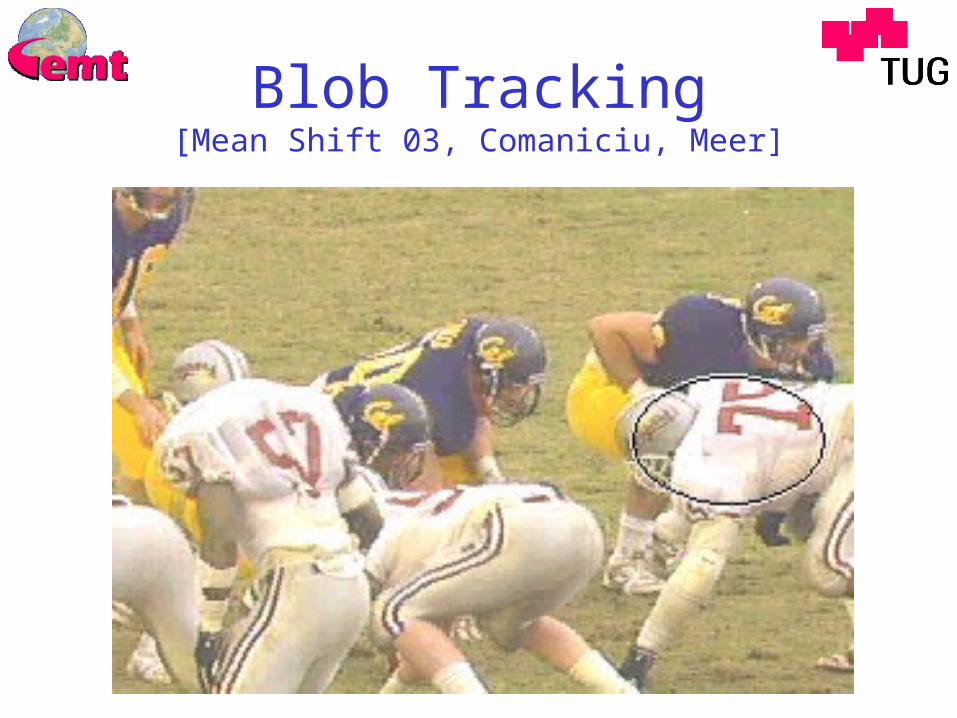
Contour Tracking[CONDENSATION 98-02, Isard, Toyama, Blake]

CONDENSATION (2)• CONditional DENSity propagATION• Requires a good initialization• Works with active contours• Maintains / adapts a contour model• Can keep more than one hypothesis

AgendaStructure of the SSIP Lecture
• Intro, terminology, applications
• 2D motion analysis
• Geometry
• 3D motion analysis
• Practical considerations
• Existing systems
• Summary, conclusions
Geometry
• Having motion in images:– What does it mean?– What can be measured?
• Projective camera• Algebraic projective geometry• Camera calibration• Computer Vision
– Reconstruction from uncalibrated views
• There are excellent textbooks[Faugeras 1994, Hartley+Zisserman 2001, Ma et al. 2003]

Projective Camera (1)• Pinhole camera model:
– p = (x,y)T is the image of P = (X,Y,Z )T – (x,y) ... image-, (X,Y,Z) ... scene-coordinates– o ... center of projection– (x,y,z) ... camera coordinate system– (x,y,-f) ... image plane
xx
yz
y
f
p(x,y)
P(X,Y,Z)
o
X
Y
Z

Projective Camera (2)• Pinhole camera model:
– If scene- = camera-coordinate system
Z
Yfy
Z
Xfx ,
Zof
x
X

Projective Camera (3)• Frontal pinhole camera model:
– (x,y,+f) ... image plane– Normalized camera: f=+1
Z
Yfy
Z
Xfx ,
xx
yzy
f
p
P(X,Y,Z)
o
X
Y
Z

Projective Camera (4)
• “real” camera:– 5 Intrinsic parameters (K)– Lens distortion– 6 Extrinsic parameters (M: R, t)
… arbitrary scale
10100
0010
0001
1Z
Y
X
y
x
MK
100
0 0
0
vfs
ufsfs
y
x
K

Algebraic Projective Geometry [Semple&Kneebone 52]
• Homogeneous coordinates
• Duality points lines
• Homography H describes any transformation– E.g.: image image transform: x’ = Hx– All transforms can be described by 3x3 matrices– Combination of transformations: Matrix product
1100
10
01
1
'
'
y
x
b
a
y
x
1100
0cossin
0sincos
1
'
'
y
x
y
x
Translation Rotation

Camera Calibration (1)
• Recover the 11 camera parameters:– 5 Intrinsic parameters (K: fsx, fsy, fs, u0, v0)
– 6 Extrinsic parameters (M: R, t)
• Calibration target:– At least 6 point correspondences – System of linear equations
• Direct (initial) solution for K and M
10100
0010
0001
~
1Z
Y
X
y
x
MK
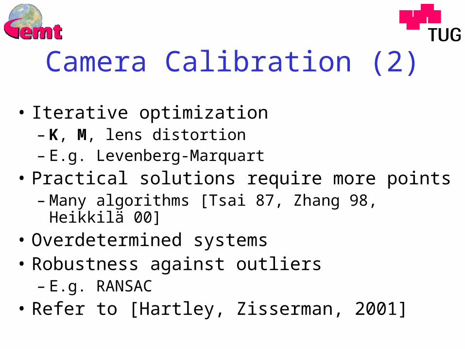
Camera Calibration (2)
• Iterative optimization– K, M, lens distortion– E.g. Levenberg-Marquart
• Practical solutions require more points– Many algorithms [Tsai 87, Zhang 98, Heikkilä 00]
• Overdetermined systems• Robustness against outliers
– E.g. RANSAC
• Refer to [Hartley, Zisserman, 2001]

What can be measured ...
• … with a calibrated camera– Viewing directions– Angles between viewing directions– 3D reconstruction: more than 1 view required
• … with uncalibrated camera(s)– Computer Vision research of the past decade– Hierarchy of geometries:
Projective – oriented projective – affine – similarity – Euclidean

AgendaStructure of the SSIP Lecture
• Intro, terminology, applications
• 2D motion analysis
• Geometry
• 3D motion analysis
• Practical considerations
• Existing systems
• Summary, conclusions

3D Motion Analysis:Location and Orientation
R
t
headcoord.system
scenecoord.system
6 DoF pose in real-timeExtrinsic parameters in real-time
3D Motion Analysis:
• Tracking technologies, terminology
• Camera pose (PnP)
• Stereo, E, F, epipolar geometry
• Model-based tracking– Confluence of 2D and 3D
• Fusion
• Kalman Filter

Tracking Technologies (1)
• Mechanical tracking
• “Magnetic tracking”
• Acoustic – time of flight
• “Optical” vision-based
• Compass
• GPS, … External effort required !No „self-contained“ system
[Allen, Bishop, Welch. Tracking: Beyond 15 minutes of thought. SIGGRAPH’01]

Tracking Technologies (2)Examples
[Allen, Bishop, Welch. Tracking: Beyond 15 minutes of thought. SIGGRAPH’01]

Research at EMT:
Hybrid Tracking – HT
Combine 2 technologies:• Vision-based
+ Good results for slow motion– Motion blur, occlusion, wrong matches
• Inertial+ Good results for fast motion– Drift, noise, long term stability
• Fusion of complementary sensors !
Mimicks human cognition !

Vision-Based Tracking More Terminology
• Measure position and orientation in real-time• Obtain trajectories of object(s)• Moving observer, egomotion – “inside-out”• Stationary observer – “outside-in Tracking”• Combinations of the above• Degrees of Freedom – DoF
– 3 DoF (mobile robot)– 6 DoF (head tracking in AR)

Inside-out Tracking
• monocular• exterior parameters• 6 DoF from 4 points• wearable, fully mobile
corners blobs natural landmarks

Outside-in Tracking
stereo-rigIR-illumination
• no cables
• 1 marker/device:3 DoF
• 2 markers: 5 DoF• 3 markers: 6 DoF
devices

Camera Pose Estimation
• Pose estimation: Estimate extrinsic parameters from known / unknown scene find R, t
• Linear algorithms [Quan, Zan, 1999]• Iterative algorithms [Lu et al., 2000]
• Point-based methods– No geometry, just 3D points
• Model-based methods– Object-model, e.g. CAD

PnP(1)Perspective n-Point Problem
• Calibrated camera K, C = (KKT)-1
• n point correspondences scene image
• Known scene coordinates of pi, and known distances dij = || pi – pj ||
• Each pair (pi,pj) defines an angle can be measured (2 lines of sight,
calibrated camera)
constraint for the distance ||c – pi||c
xi xj
pi pj
dij

PnP (2)
jTji
Ti
jTi
ij
ijjijijiij
ijjiji
jjii
CC
C
dxxxxxxf
xxxxd
xx
uuuu
uu
cpcp
cos :camera calibrated
0cos2),(
cos2 :constraint
, :searching
2ij
22
222ij
c
xi xj
pi pj
uiuj
dij

PnP (3)• P3P, 3 points:
underdetermined, 4 solutions
• P4P, 4 points:
overdetermined, 6 equations, 4 unknowns
4 x P3P, then find a common solution
• General problem: PnP, n points
0),(
0),(
0),(
3223
3113
2112
xxf
xxf
xxf
4,3,2
4,3,1
4,2,1
3,2,1

PnP (4)
Once the xi have been solved:
1) project image points scene
p’i = xi K-1 ui
2) find a common R, t for p’i pi
(point-correspondences solve a simple system of linear equations)

Stereo Reconstruction
Elementary stereo geometryin “canonical configuration”
2 h … “baseline” b
Pr - Pl … “disparity” d
There is just column disparity
Depth computation:
d
bfPz
x
z
y
hh
x=0 xr=0xl=0
f
Pl Pr
Cl Cr
P(x,y,z)
Pz

Stereo (2)
• 2 cameras, general configuration: Epipolar geometry
Cl Cr
X
ulur
ll lr
el er
Y
v

• Uncalibrated cameras: Fundamental matrix F
• Calibrated cameras: Essential matrix E
• 3x3, Rank 2
• Many Algorithms– Normalized 8-point [Hartley 97]– 5-point (structure and motion) [Nister 03]
Stereo (3)
1111 )()( rT
lrT
l EKKSRKKF
0rTl Fuu

Model-Based TrackingConfluence of 2D and 3D [Deutscher, Davison, Reid 01]

3D Motion Analysis:
• Tracking technologies, terminology
• Camera pose (PnP)
• Stereo, E, F, epipolar geometry
• Model-based tracking– Confluence of 2D and 3D
• Fusion
• Kalman Filter1. General considerations2. Kalman Filter EMT HT project

General Considerations• We have:
– Several sensors (vision, inertial, ...)– Algorithms to deliver pose streams for each sensor
(at discrete times; rates may vary depending on sensor, processor, load, ...)
• Thus, we need:– Algorithms for sensor fusion (weighting the
confidence in a sensor, sensor accuracy, ...)– Pose estimation including a temporal model
[Allen, Bishop, Welch. Tracking: Beyond 15 minutes of thought. SIGGRAPH’01]

Sensor Fusion
• Dealing with ignorance:– Imprecision, ambiguity, contradiction, ...
• Mathematical models– Fuzzy sets– Dempster-Shafer evidence theory– Probability theory
• Probabilistic modeling in Computer Vision– The topic of this decade !– Examples: CONDENSATION, mean shift

Kalman Filter (1)
http://www.cs.unc.edu/~welch/kalman[Welch, Bishop. An Introduction to the Kalman Filter. SIGGRAPH’01]

Kalman Filter (2)
• Estimate a process
• with a measurement11 kkkk wBuAxx
kkk vHxz
xn ... State of the process zm ... Measurementp, v ... Process and measurement noise (zero mean)A ... n x n Matrix relates the previous with the current time stepB ... n x l Matrix relates optional control input u to xH ... n x m Matrix relates state x to measurement z
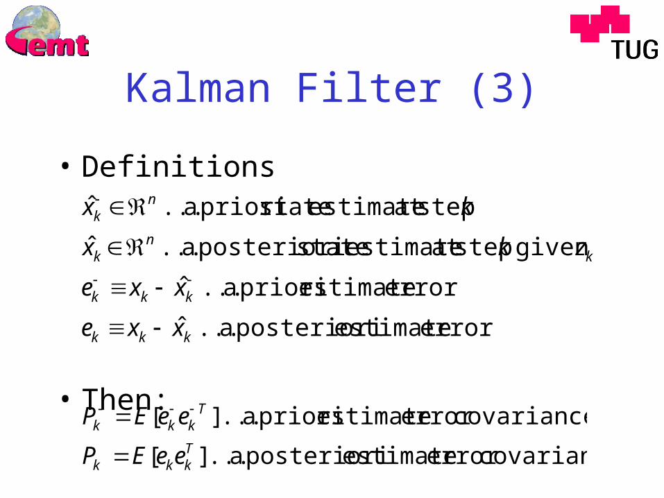
Kalman Filter (3)
• Definitions
• Then:
error estimate posterioria ... ˆ
error estimate prioria ... ˆ
given stepat estimate state posterioria ... ˆ
stepat estimate state prioria ... ˆ
kkk
kkk
kn
k
nk
xxe
xxe
zkx
kx
covarianceerror estimate posterioria ... ][
covarianceerror estimate prioria ... ][Tkkk
Tkkk
eeEP
eeEP

Kalman Filter (4)
• Compute
• with
k
kk
kkkk
PmnK
xHz
xHzKxx
minimizes that gain" Kalman" ...
"innovationt measuremen" ... )ˆ(
)ˆ(ˆˆ
covarianceerror nt Measureme...
)( 1
R
RHHPHPK Tk
Tkk

Kalman Filter (5)
http://www.cs.unc.edu/~welch/kalman

Kalman Filter (6)
http://www.cs.unc.edu/~welch/kalman
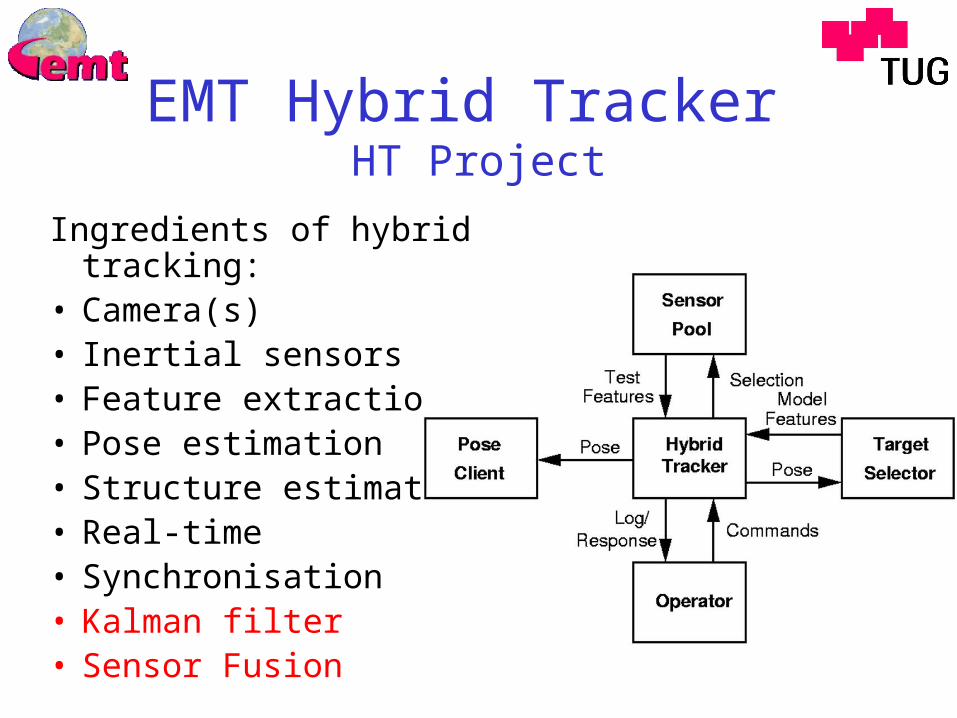
EMT Hybrid Tracker HT Project
Ingredients of hybrid tracking:• Camera(s)• Inertial sensors• Feature extraction• Pose estimation• Structure estimation• Real-time• Synchronisation• Kalman filter• Sensor Fusion

Hybrid Tracking
• 6 DoF vision-based tracker
• 6 DoF inertial tracker
• Fusion by a Kalman filter

“Structure and Motion”
“Tracking” + “Structure from Motion”

Research Prototype
• Tracking subsystem• Visualization subsystem• Sensors + HMD

HT Application Example
AgendaStructure of the SSIP Lecture
• Intro, terminology, applications
• 2D motion analysis
• Geometry
• 3D motion analysis
• Practical considerations
• Existing systems
• Summary, conclusions

Practical Considerations
• There are critical configurations !• Projective geometry vs. discrete pixels
– Rays do not intersect !– Error minimization algorithms required
• Robustness (many points) vs. real-time– Outlier detection can become difficult !
• Precision (iterative) vs. real-time (linear)• Combination of diverse features
– Points, lines, curves
• Jitter, lag• Debugging of a real-time system !

Existing Systems (1)• VR/AR
– Intersense, Polhemus, A.R.T.
• MoCap– Vicon, A.R.T.
• Medical tracking– MedTronic, A.R.T.
• Fiducial tracker (Intersense)• Research systems
– KLT (Kanade, Lucas, Tomasi)– ARToolkit (Billinghurst)– XVision (Hager)

Existing Systems (2)

Open Issues
• Tracking of natural landmarks
• First success in online structure and motion– [Nister CVPR03, ICCV03, ECCV04]
• (Re-)Initialisation in highly complex scenes
• Usability !

Future Applications• Can pose (position and orientation) be exploited ?
– What is the user looking at?– Architecture, city guide, museum, emergency, …
• From bulky gear and HMD PDA– Wireless communication– Camera(s)– Inertial sensors (+ compass, + GPS, …)
• Automotive !– Driver assistance– Autonomous vehicles, mobile robot navigation, …
• Medicine !– Surgical navigation – Online fusion (temporal genesis, sensory modes, …)

Summary, Conclusions
• Real-time pose (6 DoF)
• 2D and 3D motion analysis
• Geometry
• Probabilistic modeling
• High potential for future developments

Acknowledgements
• EU-IST-2001-34401 Vampire - Visual Active Memory Processes and Interactive Retrieval
• FWF P15748 Smart Tracking• FWF P14470 Mobile
Collaborative AR• Christian Doppler Laboratory for
Automotive Measurement Research
• Markus Brandner• Harald Ganster• Bettina Halder• Jochen Lackner• Peter Lang• Ulrich Mühlmann• Miguel Ribo• Hannes Siegl• Christoph Stock• Georg Teichtmeister• Jürgen Wolf

Further Reading
R. Hartley, A. Zisserman. Multiple View Geometry in Computer Vision. Cambridge University Press, 2nd ed., 2003.
Y. Ma, S. Soatto, J. Kosecka, S. Shankar Sastry. An Invitation to 3D Vision.Springer, 2004.
B.D. Allen, G. Bishop, G. Welch. Tracking: Beyond 15 Minutes of Thought.SIGGRAPH 2001, Course 11. See http://www.cs.unc.edu/~welch
G. Welch, G. Bishop. An Introduction to the Kalman Filter. SIGGRAPH 2001, Course 8. See http://www.cs.unc.edu/~welch