Real-World Uplift Modelling with Signiﬁcance-Based Uplift ...stochasticsolutions.com/pdf/sig-based-up-trees.pdf · Real-World Uplift Modelling with Signiﬁcance-Based Uplift Trees

Real-World Uplift Modelling withSignificance-Based Uplift Trees

Nicholas J. Radcliffea,b

& Patrick D. Surryc

[email protected]

[email protected]

aStochastic Solutions Limited, 37 Queen Street, Edinburgh, EH2 1JX, UK.bDepartment of Mathematics, University of Edinburgh, King’s Buildings, EH9 3JZ.

cPitney Bowes Business Insight, 125 Summer Street, 16th Floor, Boston, MA 02110, USA.

Abstract

This paper seeks to document the current state of the art in ‘uplift modelling’—thepractice of modelling the change in behaviour that results directly from a specifiedtreatment such as a marketing intervention. We include details of the Significance-Based Uplift Trees that have formed the core of the only packaged uplift mod-elling software currently available. The paper includes a summary of some ofthe results that have been delivered using uplift modelling in practice, with ex-amples drawn from demand-stimulation and customer-retention applications. Italso surveys and discusses approaches to each of the major stages involved in up-lift modelling—variable selection, model construction, quality measures and post-campaign evaluation—all of which require different approaches from traditionalresponse modelling.

1 OrganizationWe begin by motivating and defining uplift modelling in section 2, then review thehistory and literature of uplift modelling (section 3), including a review of results.Next, we devote sections, in turn, to four key areas involved in building and usinguplift models. We start with the definition of quality measures and success criteria(section 4), since these are a conceptual prerequisite for all of the other areas. Wethen move on to the central issue of model construction, first discussing a number ofpossible approaches (section 5), and then detailing the core tree-based algorithm thatwe have used successfully over a number of years, which we call the Significance-Based Uplift Tree (section 6). Next, we address variable selection (section 7). Thisis important because the best variables for conventional models are not necessarily thebest ones for predicting uplift (and, in practice, are often not). We close the main bodywith some final remarks (section 8), mostly concerning when, in practice, an upliftmodelling approach is likely to deliver worthwhile extra value.

1

Real-World Uplift Modelling with Significance-Based Uplift Trees Radcliffe & Surry

2 Introduction

2.1 Predictive Modelling in Customer ManagementStatistical modelling has been applied to problems in customer management since theintroduction of statistical credit scoring in the early 1950s, when the consultancy thatbecame the Fair Isaac Corporation was formed (Thomas, 2000).1 This was followedby progressively more sophisticated use of predictive modelling for customer targeting,particularly in the areas of demand stimulation and customer retention.

As a broad progression over time, we have seen:

1. penetration (or lookalike) models, which seek to characterize the customers whohave already bought a product. Their use is based on the assumption that peo-ple with similar characteristics to those who have already bought will be goodtargets, an assumption that tends to have greatest validity in markets that are farfrom saturation;

2. purchase models, which seek to characterize the customers who have bought ina recent historical period. These are similar to penetration models, but restrictattention to the more recent past. As a result, they can be more sensitive tochanges in customer characteristics across the product purchase cycle from earlyadopters through the mainstream majority to laggards (Moore, 1991);

3. ‘response’ models, which seek to characterize the customers who have purchasedin apparent ‘response’ to some (direct) marketing activity such as a piece of di-rect mail. Sometimes, the identification of ‘responders’ involves a coupon, ora response code (‘direct attribution’), while in other cases it is simply based ona combination of the customer’s having received the communication and pur-chasing in some constrained time window afterwards2 (‘indirect attribution’).‘Response’ models are normally considered to be more sophisticated than bothpenetration models and purchase models, in that they at least attempt to con-nect the purchase outcome with the marketing activity designed to stimulate thatactivity.

All of these kinds of modelling come under the general umbrella of ‘propensity mod-elling’.

In the context of customer retention, there has been a similar progression, startingwith targeted acquisition programmes, followed by models to predict which customersare most likely to leave, particularly around contract renewal time. Such ‘churn’ or ‘at-trition’ models are now commonly combined with value estimates allowing companiesto focus more accurately on retaining value rather than mere customer numbers.

1Thomas reports that David Durand of the US National Bureau of Economic Research was the first tosuggest the idea of applying statistical modelling to predicting credit risk (Durand, 1941).

2More complex inferred response rules are sometime used to attribute particular sales to given marketingtreatments, but these appear to us to be rather hard to justify in most cases.

Portrait Technical Report TR-2011-1 2 Stochastic Solutions White Paper 2011


2.2 Measuring Success in Direct Marketing: the Control GroupThe primary goal of most direct marketing is to effect some specific change in customerbehaviour. A common example of this is the stimulation of extra purchasing by a groupof customers or prospects. While there may be subsidiary goals, such as brand aware-ness and the generation of customer goodwill, most marketing campaigns are primarilyevaluated on the basis of some kind of return-on-investment (ROI) calculation.

If we focus, initially, on the specific goal of generating incremental revenue, it isclear that measurement of success is non-trivial, because of the difficulty of knowingwhat level of sales would have been achieved had the marketing activity in questionnot been undertaken. The key, as is well known, is the use of a control group, andit is a well-established and widely recognized best practice to measure the incremen-tal impact of direct marketing activity by comparing the performance of the treatedgroup with that of a valid control group chosen uniformly at random3 from the targetpopulation.

2.3 The Uplift Critique of Conventional Propensity ModellingWhile there is a broad consensus that accurate measurement of the impact of directmarketing activity requires a focus on incrementality through the systematic and carefuluse of control groups, there has been much less widespread recognition of the need tofocus on incrementality when selecting a target population. None of the approaches topropensity modelling discussed in section 2.1 is designed to model incremental impact.Thus, perversely,

most targeted marketing activity today, even when measured on the basisof incremental impact, is targeted on the basis of non-incremental models.

It is widely recognized that neither penetration models nor purchase models even at-tempt to model changes in customer behaviour, but less widely recognized that so-called ‘response’ models are also not designed to model incremental impact. The rea-son they do not is that the outcome variable4 is necessarily set on the basis of a testsuch as “purchased within a 6-week period after the mail was sent” or the use of somekind of a coupon, code or custom link. Such approaches attempt to tie the purchaseto the campaign activity, either temporally or through a code. But while these providesome evidence that a customer has been influenced by (or was at least aware of) themarketing activity, they by no means guarantee that we limit ourselves to incrementalpurchasers. These approaches can also fail to record genuinely incremental purchasesfrom customers who have been influenced but for whatever reason do not use the rele-vant coupon or code.

For the same reasons that we reject as flawed measurement of the incrementality ofa marketing action through counting response codes or counting all purchases within

3Strictly, the control group does not have to be chosen in this way. It can certainly be stratified, andcan even be from a biased distribution if that distribution is known, but this is rarely done as it complicatesthe analysis considerably. Although we have sometimes used more complicated test designs, for clarity ofexposition, we assume uniform random sampling throughout this paper.

4the dependent variable, or target variable



a time window, we must reject as flawed modelling based on outcomes that are notincremental if our goal is to model the change in behaviour that results from a givenmarketing intervention (as it surely should be if our success metric is incremental).

A common case worth singling out arises when a response code is associated with adiscount or other incentive. If a customer who has already decided to buy a given itemreceives a coupon offering a discount on that item, it seems likely that in many cases thecustomer will choose to use the coupon. (Indeed, it is not uncommon for helpful salesstaff to point out coupons and offers to customers.) Manifestly, in these cases, the salesare not incremental5 whatever the code on coupon may appear to indicate. Indeed,in this case, not only were marketing costs increased by including the customer, butincremental revenue was reduced—from some perspectives, almost the worst possibleoutcome.

2.4 The Unfortunately Named ‘Response’ ModelWe suspect that the very term ‘response modelling’ is a significant impediment to thewider appreciation of the fact that so-called ‘response models’ in marketing are notreliably incremental. The term ‘response’ is (deliberately) loaded and carries the un-mistakable connotation of causality. At the risk of labouring the point, the OxfordEnglish Dictionary’s first definition (Onions, 1973, p. 1810) of response is:

Response. 1. An answer, a reply. b. transf. and fig. An action or feelingwhich answers to some stimulus or influence.

While it is unrealistic for us to expect to change the historic and accepted nomencla-ture, we encourage the term ‘response’ model to be used with care and qualification.As noted before, our preferred term for models that genuinely model the incrementalimpact of an action is an ‘uplift model’, though as we shall see, other terms are alsoused.

2.5 Conventional Models and Uplift ModelsAssume we partition our candidate population randomly6 into two subpopulations, TandC. We then apply a given treatment to the members of T and not toC. Consideringfirst the binary case, we denote the outcome O ∈ {0, 1}, and here assume that 1 is thedesirable outcome (say purchase).

A conventional ‘response’ model predicts the probability that O is 1 for customersin T . Thus a conventional model fits

P (O = 1 | x;T ), (conventional binary ‘response’ model) (1)

5We are assuming here that the coupon was issued by the manufacturer, who is indifferent as to thechannel through which the item is purchased. A coupon from a particular shop could cause the customer toswitch to that shop, but again the coupon alone does not establish this, as the customer could and might havebought from that shop anyway.

6When we say randomly, we more precisely mean uniformly, at random, i.e. each member of the pop-ulation is assigned to T or C independently, at random, with some fixed, common probability p ∈ (0, 1)



where P (O = 1 | x;T ) denotes “the probability that O = 1 given that the customer,described by a vector of variables x, is in subpopulation T ”. Note that the control groupC does not play any part of this definition. In contrast, an uplift model fits

P (O = 1 | x;T )− P (O = 1 | x;C). (binary uplift model) (2)

Thus, where a conventional ‘response’ model attempts to estimate the probability thatcustomers will purchase if we treat them, an uplift model attempts to estimate the in-crease in their purchase probability if we treat them over the corresponding probabilityif we do not. The explicit goal is now to model the difference in purchasing behaviourbetween T and C.

Henceforth, we will not explicitly list the x dependence in equations such as these,but it should be assumed.

We can make an equivalent distinction for non-binary outcomes. For example, ifthe outcome of interest is some measure of the size of purchase, e.g, revenue, R, theconventional model fits

E(R | T ) (conventional continuous ‘response’ model) (3)

whereas the uplift model estimates

E(R | T )− E(R | C) (continuous uplift model) (4)

3 History & Literature ReviewThe authors’ interest in predicting incremental response began around 1996 while con-sulting and building commercial software for analytical marketing.7 At that time, themost widely used modelling methods for targeting were various forms of regressionand trees.8 The more common regression methods included linear regression, logisticregression and generalised additive models (Hastie & Tinshirani, 1990), usually in theform of scorecards. Favoured tree-based methods included classification and regres-sion trees (CART; Breiman et al., 1984) and, to a lesser extent, ID3 (Quinlan, 1986),C4.5 (Quinlan, 1993), and AID/CHAID (Hawkins & Kass, 1982; Kass, 1980). Thesewere used to build propensity models, as described in the introduction. It quickly be-came clear to us that these did not lead to an optimal allocation of direct marketingresources for reasons described already, with the consequence that they did not allowus to target accurately the people who were most positively influenced by a marketingtreatment.

We developed a series of tree-based algorithms for tackling uplift modelling, all ofwhich were based on the general framework common to most binary tree-based meth-ods (e.g. CART), but using modified split criteria and quality measures. Tree methods

7The Decisionhouse software was produced by Quadstone Limited, which is now part of Pitney Bowes.8Both of these classes of methods remain widely used, though they have been augmented by recommen-

dation systems that focus more on product set rather than other customer attributes, using a variety of meth-ods including collaborative filtering (Resnick et al., 1994) and association rules (Piatetsky-Shapiro 1991).Bayesian approaches, particularly Naı̈ve Bayes models (Hand & Yu, 2001), have also grown in popularityover this period.



usually begin with a growth phase employing a greedy algorithm (Cormen et al., 1990).Such greedy algorithms start with the whole population at the root of the tree and thenevaluate a large number of candidate splits, using an appropriate quality measure. Thestandard approach considers a number of splits for each (potential) predictor.9 The bestsplit is then chosen and the process is repeated recursively (and independently) for eachsubpopulation until some termination criterion is met—usually once the tree is large.In many variants, there is then a pruning phase during which some of the lower splitsare discarded in the interest of avoiding overfitting. The present authors outlined ourapproach in a 1999 paper (Radcliffe & Surry, 1999), when we used the term DifferentialResponse Modelling to describe what we now call Uplift Modelling.10 At that point,we did not publish our (then) split criterion, but we now give details of our current, im-proved criterion in section 6. Other researchers have developed alternative methods forthe same problem independently, unfortunately using different terminology in almostevery case.

Various results from the approach described in this paper have been published else-where, including:

• US Bank found that a ‘response’ model was spectacularly unsuccessful for tar-geting a (physical) mailshot promoting a high-value product to its existing cus-tomers. When the whole base was targeted, this was profitable (on the basisof the value of incremental sales measured against a control group), but whenthe top 30% identified by a conventional ‘response’ model was targeted, the re-sult was almost exactly zero incremental sales (and a resulting negative ROI).This was because the ‘response’ model succeeded only in targeting people whowould have bought anyway. An uplift model managed to identify a different30% which, when targeted, generated 90% of the incremental sales achievedwhen targeting the whole population, and correspondingly turned a severely loss-making marketing activity into a highly successful (and profitable) one (Grund-hoefer, 2009).11

• A mobile churn reduction initiative actually increased churn from 9% to 10%prior to uplift modelling. The uplift model allowed a 30% subsegment to beidentified. Targeting only that subsegment reduced overall churn from 9% tounder 8%, while reducing spend by 70% (Radcliffe & Simpson, 2008). Theestimated value of this to the provider was $8m per year per million customersin the subscriber base.

• A different mobile churn reduction initiative (at a different operator) was suc-cessful in reducing churn by about 5 percentage points (pp), but an uplift modelwas able to identify 25% of the population where the activity was marginal or

9independent variable10Various versions of the algorithm were implemented in the Decisionhouse software over the years, and

used commercially, with increasing success.11US Bank also developed an in-house approach to uplift prediction called a matrix model. This was based

on the idea of comparing predictions from a response model on the treated population with a natural buy ratemodel built on a mixed population. Prediction from both models were binned and segments showing highuplift were targeted. This produced a somewhat useful model, but one that was less than half as powerful asa direct, significance tree-based uplift model.



counterproductive. By targeting only the identified 75% overall retention was in-creased by from 5 pp to 6 pp, (i.e. 20% more customers were saved) at reducedcost (Radcliffe & Simpson, 2008). This was also valued at roughly $8m per yearper million customers in the subscriber base.

We also published an electronic retail analysis based on a challenge set by Kevin Hill-strom (Radcliffe, 2008) of MineThatData (Hillstrom, 2008).

Maxwell et al. (2000), at Microsoft Research, describe their approach to targetingmail to try to sell a service such as MSN. Like us, they base their approach on decisiontrees but they simply build a standard tree on the whole population (treated and control)and then force a split on the treatment variable at each leaf node. The primary limitationwith this approach is that splits in the tree are not chosen to fit uplift; it is simplythe estimation at the end that is adapted. The authors do not compare to a non-upliftalgorithm, but report benefits over a mail-to-all strategy in the range $0.05 to $0.20 perhead.

Hansotia & Rukstales (2001, 2002) describe their approach to what they call In-cremental Value Modelling, which involves using the difference in raw uplifts in thetwo subpopulations as a split criterion. This, indeed, is a natural approach but hasthe obvious disadvantage that population size is not taken into account, leading to anoveremphasis on small populations with high observed uplift in the training population.

Lo (2002) has maintained a long-term interest in what he calls True Lift Modellingwhile working in direct marketing for Fidelity Investments. He developed an approachwhich is based on adding explicit interaction terms between each predictor and thetreatment. Having added these terms he performs a standard regression. To use themodel, he computes the prediction with the treatment variable set to one (indicatingtreatment) and subtracts the prediction from the model with the treatment variable setto zero. Lo has used this approach to underpin direct marketing at Fidelity for a numberof years (Lo, 2005) with good success.

Manahan (2005) tackles the problem from the perspective of a cellular phone com-pany (Cingular) trying to target customers for retention activity around contract renewaltime. As Manahan notes, an extra reason for paying attention in this case is that thereis clear evidence that retention activity backfires for some customers and has the neteffect of driving them away. Manahan calls his method a Proportional Hazards ap-proach, and the paper is couched in terms of survival analysis (hence the ‘hazards’language), but on close reading it appears that the core method for predicting upliftis, like Hansotia & Rukstales (2001), the ‘two-model’ approach, i.e. direct subtrac-tion of models for the treated and untreated populations. Manahan uses both logisticregression and neural network models, and finds that in his case the neural approachis more successful. (Manahan creates rolling predictions of customer defection ratesfrom his uplift models and compares these with known survival curves both as a formof validation and an input to model selection.)

As well as these published approaches, we have seen many organizations try thenatural approach of modelling the two populations (treated and control) separately andsubtracting the predictions. This has the advantages of simplicity and manifest correct-ness. Unfortunately, as we discuss in section 5, in our experience, in all but the simplestcases it tends to fail rather badly. (We refer to this as the ‘two-model’ approach to uplift



modelling.)More recently, Larsen (2010) has reported work at Charles Schwab using what he

calls Net Lift Modeling. His approach is much closer to ours in that it fundamentallychanges the quantity being optimized in the fitting process to be uplift (net lift). He doesthis using a modification of the weight of evidence transformation (Thomas, 2000) toproduce the net weight of evidence, which is then used as the basis of fitting using eithera K-Nearest Neighbours approach (Hand, 1981) or a Naı̈ve Bayes approach (Hand &Yu, 2001). Larsen also proposes using a net version of ‘information value’ (the netinformation value) for variable selection.

Finally, Rzepakowski & Jaroszewicz (2010) have proposed a tree-based method foruplift modelling that is based on generalizing classical tree-building split criteria andpruning methods. Their approach is fundamentally based on the idea of comparingthe distributions of outcomes in the treated and control populations using a divergencestatistic and they consider two, one based on the Kullback-Leibler divergence and an-other based on a Euclidean metric. Although we have not performed an experimentalcomparison yet, we note that their approach is designed partly around a postulate stat-ing that if the control group is empty the split criterion should reduce to a classicalsplitting criterion. This does not seem natural to us; a more appropriate requirementmight be that when the response rate in the control population is zero the split crite-rion should reduce to a classical case. We are also concerned that their proposed splitconditions are independent of overall population size, whereas our experience is thatthis is critical in noisy, real-world situations. Finally, it is troubling that the standarddefinition of uplift (as the difference between treated and control outcome rates) cannotbe used in their split criterion because of an implicit requirement that the measure ofdistribution divergence be convex.

4 Quality Measures and Success CriteriaGiven a valid control group, computing the uplift achieved in a campaign is straightfor-ward, though subject to relatively large measurement error. Assessing the performanceof an (uplift) model is more complex.

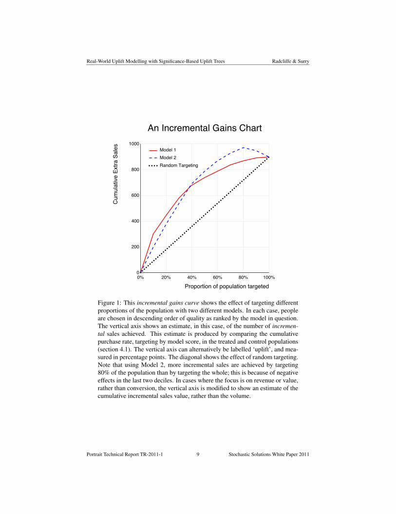
We have found the uplift equivalent of a gains curve, as shown in Figure 1, to bea useful starting point when assessing model quality (Radcliffe, 2007; Surry & Rad-cliffe, 2011). Such incremental gains curves are similar to conventional gains curvesexcept that they show an estimate of the cumulative incremental impact on the verticalaxis where the conventional gains curve shows the cumulative raw outcome.

If we have predetermined a cut-off (e.g. 20%), we can use the uplift directly asa measure of model quality: in this case, Model 1 is superior12 at 20% target volumebecause it delivers an estimated 450 incremental sales against the estimated 380 in-cremental sales delivered by Model 2. At target volumes above 40%, the situationreverses.

12For simplicity, we are not specifying, here, whether this is training or validation data, nor are we specify-ing error bars, though we would do so in practice, giving more weight to validation performance and takinginto account estimated errors.



An Incremental Gains ChartC

umul

ativ

e Ex

tra S

ales

Proportion of population targeted0% 20% 40% 60% 80% 100%0

200

400

600

800

1000Model 1Model 2Random Targeting

Figure 1: This incremental gains curve shows the effect of targeting differentproportions of the population with two different models. In each case, peopleare chosen in descending order of quality as ranked by the model in question.The vertical axis shows an estimate, in this case, of the number of incremen-tal sales achieved. This estimate is produced by comparing the cumulativepurchase rate, targeting by model score, in the treated and control populations(section 4.1). The vertical axis can alternatively be labelled ‘uplift’, and mea-sured in percentage points. The diagonal shows the effect of random targeting.Note that using Model 2, more incremental sales are achieved by targeting80% of the population than by targeting the whole; this is because of negativeeffects in the last two deciles. In cases where the focus is on revenue or value,rather than conversion, the vertical axis is modified to show an estimate of thecumulative incremental sales value, rather than the volume.



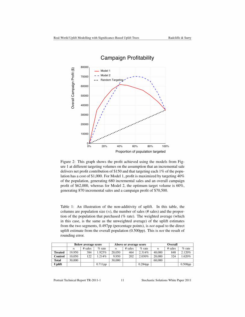
Given cost and value information, we can determine the optimal cutoff for eachmodel and choose the one that leads to the highest predicted campaign profit. Figure 2is derived directly from the incremental gains curve by applying cost and value infor-mation, illustrated here with the cost of treating each 1% of the population set to $1,000and the profit contribution from each incremental sale set to $150. Using these figures,we can go further and say that Model 2 is better in the sense that it allows us to delivera higher (estimated) overall campaign profit (c. $70,000 at 60%, against a maximum ofslightly over $60,000 at 40% for Model 1), if that is the goal.13

Since Model 1 performs better than Model 2 at small volumes while Model 2 per-forms better than Model 1 (by a larger margin) at higher target volumes, we mightborrow the notion of dominance from multi-objective optimization (Louis & Rawl-ins, 1993), and say that neither model dominates the other (i.e. neither is better at allcutoffs).

Notwithstanding the observation that different models may outperform each otherat different target volumes, it is useful to have access to measures that summarizeperformance across all possible target volumes. Qini measures (Radcliffe, 2007) dothis, and we will outline them below after a few introductory points.

4.1 Segment-based vs. Pointwise Uplift Estimates: Non-AdditivityThe core complication with uplift modelling lies in the fact that we cannot measure theuplift for an individual because we cannot simultaneously treat and not treat a singleperson. For this reason, developing any useful quality measure based on comparingactual and observed outcomes at the level of the individual seems doomed to failure.

Given a valid treatment-control structure, we can, however, estimate uplift for dif-ferent segments, provided that we take equivalent subpopulations in each of the treatedand control and that those subpopulations are large enough to be meaningful. Thisincludes the case of a population segmented by model score. Thus it is legitimate forus to estimate the uplift for customers with scores in the range (say) 100–200 by com-paring the purchase rates of customers with scores in this range from the treated andcontrol populations.

In going down this route, however, we need to be aware that uplift estimates arenot, in general, additive (see Table 1). This is because of unavoidable variation in theprecise proportions of treated and control customers in arbitrary subsegments.14

4.2 Qini MeasuresQini measures are based on the area under the incremental gains curve (e.g. Figure 1).This is a natural generalization of the gini coefficient, which though more commonlydefined with reference to the area under a receiver-operator characteristic (ROC) curve,can equivalently be defined with reference to the conventional gains curve. Because theincremental gains curve is so intimately linked to the qini measure, we tend to refer to

13This statement assumes that the uplift estimates are accurate. In general, uplift cannot be estimated asaccurately as a purchase rate can be.

14a phenomenon related to Simpson’s ‘Paradox’ (Simpson, 1951)



Campaign Profitability

Ove

rall

Cam

paig

n Pr

ofit

($)

Proportion of population targeted0% 20% 40% 60% 80% 100%0

10000

20000

30000

40000

50000

60000

70000

80000Model 1Model 2Random Targeting

Figure 2: This graph shows the profit achieved using the models from Fig-ure 1 at different targeting volumes on the assumption that an incremental saledelivers net profit contribution of $150 and that targeting each 1% of the popu-lation has a cost of $1,000. For Model 1, profit is maximized by targeting 40%of the population, generating 680 incremental sales and an overall campaignprofit of $62,000, whereas for Model 2, the optimum target volume is 60%,generating 870 incremental sales and a campaign profit of $70,500.

Table 1: An illustration of the non-additivity of uplift. In this table, thecolumns are population size (n), the number of sales (# sales) and the propor-tion of the population that purchased (% rate). The weighted average (whichin this case, is the same as the unweighted average) of the uplift estimatesfrom the two segments, 0.497pp (percentage points), is not equal to the directuplift estimate from the overall population (0.500pp). This is not the result ofrounding error.

Below average score Above or average score Overalln # sales % rate n # sales % rate n # sales % rate

Treated 19,950 384 1.925% 20,050 464 2.314% 40,000 848 2.120%Control 10,050 122 1.214% 9,950 202 2.030% 20,000 324 1.620%Total 30,000 30,000 60,000Uplift 0.711pp 0.284pp 0.500pp



the curve on an incremental gains graph as a qini curve. Qini curves and qini measuresare discussed in detail in Radcliffe (2007) but key features include:

1. Gini. The gini coefficient is defined as the ratio of two areas. The numeratoris the area between the actual gains curve and the diagonal corresponding torandom targeting. The denominator is the same area but now for the optimalgains curve. This optimal gains curve is achieved by a model that assigns higherscores to all the responders than to any of the non-responders and leads to atriangular gains curve with slope 1 at the start15 and 0 after all the purchasershave been ‘used up’. Thus gini coefficients range from +1, for a model thatcorrectly ranks all purchasers ahead of all non-purchasers, to 0, for a modelthat performs as well (overall) as random targeting, to −1 for the worst possiblemodel, which ranks each non-purchaser ahead of all purchasers.

2. q0 — a direct analogue of gini. Because of the possibility of negative effects,16

even for a binary response variable, the optimum incremental gains curve is lessobvious, though can be calculated straightforwardly (details in Radcliffe, 2007).However, we do not generally use this for scaling the qini measure, partly be-cause this theoretical optimum is often an order of magnitude or more largerthan anything achievable, and partly because it is not well defined for non-binaryoutcomes. Instead, we often scale with respect to the so-called zero downlift op-timum, which is the optimal gains curve if it is assumed that there are no negativeeffects. This version of the qini coefficient is denoted by q0 and is defined as theratio of the area of the actual incremental gains curve above the diagonal to thezero-downlift incremental gains curve. It should be noted, however, that if theoverall uplift is zero, the area of the zero-downlift qini curve will also be zero,leading to an infinite result for q0.

3. Q — the more general qini measure. Although the q0 measure is a useful directanalogue of gini for binary outcomes, the more generally useful measure is theunscaled qini measure Q. This is defined simply as the area between the actualincremental gains curve in question and the diagonal corresponding to randomtargeting. This is scaled only to remove dependence on the population size N ,dividing by N2, where necessary.

4. Calculational Issues and Non-Additivity. Uplift estimates are not strictly addi-tive. For this reason, some ways of calculating the qini coefficient are moresubject to statistical variation than others (see Surry & Radcliffe, 2011).

4.3 Success Criteria and GoalsThe qini measure is the most concrete and direct measure of overall model performancewe currently have, but we need to discuss further what it means for an uplift model tobe ‘good’.

15assuming both axes use the same scaling16Negative effects arise when, for some or all segments of the population, the overall impact of the treat-

ment is to reduce sales.



With a conventional model, we can directly compare the predictions from the modelto the actual outcomes, point-by-point, both on the data used during model building andon validation data. There is no equivalent process for an uplift model.

We can directly compare the predictions of the model over different subpopulations.The qini measure does this, with the subpopulations being partially defined by thepredictions themselves, i.e. we work from the highest scores to the lowest. There isnecessarily a degree of arbitrariness in terms of exactly how we define the segments,but this is not a large problem.

The qini measure, like gini, is a measure only of the rank ordering performed bythe model. For many purposes this is sufficient, particularly in cases where there is arelatively small, fixed volume to be treated and the model is to be used simply to pickthe best candidates.

For some purposes, however, calibration matters, especially when picking cut-offpoints, i.e. sometimes the actual correspondence between the predicted uplift for asegment and the actual uplift is important.

Even perfect accuracy of predictions at segment level is no guarantee of utility ofthe model, because uplift predictions can be arbitrarily weak. For example, we coulddefine a set of random segments, and predict the population average uplift for eachof them. We would expect excellent correspondence between our useless predictionsand reality17 but the model would be of no help to use because it makes no interestingpredictions. Thus we need not only accurate predictions at segment level, but a rangeof different predictions in order for a model to have any utility.

In general, we consider all of the following when evaluating uplift models:

• Validated qini (i.e. comparing two models, the one with a higher qini on valida-tion data will generally be preferred);18

• Monotonicity of incremental gains: for reasonably large segments, we like eachsegment to have lower uplift than the previous (working from high predicteduplift to lower predicted uplift);

• Maximum impact: where negative effects are present, we have regard to thehighest predicted uplift we can achieve, especially when the incremental gainshave a stable, monotonic pattern;

• Impact at cutoff: Sometimes, the cutoff is predetermined or determined by aprofit calculation based on the predictions: in these cases, we are of course con-cerned with the performance at the cutoff.

• Tight validation: as with conventional models, we are more confident when thepattern seen in validation data is very similar to that in the data used to buildthe model (though the inherently larger errors associated with measuring upliftmean that validation is rarely as tight as with conventional models).

17compromised only by statistical variation18qini values for the same dataset and outcome are comparable, but comparing qini values across different

datasets and outcomes can be less meaningful.



• Range of Predictions. As noted, other things being equal, the more different thepredictions of the model for different segments, the more useful is the model.

When, in later sections, we describe approaches as ‘successful’ or ‘unsuccessful’ with-out specifying a criterion, we are generally referring to a combination of most or all ofthese performance considerations.

5 Approaches to Building Uplift ModelsWe first discuss the obvious ‘two-model’ approach to uplift modelling (section 5.1)and why it tends not to work well (sections 5.2 and 5.3), and some approaches basedon additive models (section 5.4). We then discuss the shared character of more fruit-ful approaches to building uplift models (section 6) before discussing the tree-basedapproach in detail (section 6.1).

5.1 The Two Model ApproachAs noted in section 3, the most straightforward approach to modelling uplift is to buildtwo separate models, one, MT , for the treated population and another, MC , for thecontrol population, and then to subtract their predictions to predict uplift (MU =MT − MC). The main advantages of this approach are (1) simplicity (2) manifestcorrectness in principle and (3) lack of requirement for new methods, techniques andsoftware. Unfortunately, while the approach works well in simple cases, such as areoften constructed as tests, our experience and that of others (e.g. Lo, 2002) is that thisapproach rarely works well for real-world problems. We will now attempt to explainwhy this should be the case, accepting that our explanation will be partial because thereis much that is still not understood about uplift modelling.

The authors believe that multiple factors contribute to the practical failure of thetwo-model approach in real-world situations:

1. Objective. The two-model approach builds two independent models, usuallyon the same basis, using the same model form and candidate predictors. Eachis fitted on the basis of a fitting objective that makes no reference to the otherpopulation. Thus, viewed from an optimization perspective, when we build twoseparate models, nothing in the fitting process is (explicitly) attempting to fit thedifference in behaviour between the two populations.

In effect, this approach is based upon the (correct) observation that if the twomodels were perfect, in the sense of making correct predictions for every cus-tomer under both treated and control scenarios, then the uplift prediction formedby subtracting them would also be perfect. It does not, however, follow that sub-tracting two ‘good’ independent models will necessarily lead to a ‘good’ upliftmodel. (Before we could even assign meaning to such a statement, we wouldfirst need to define our metrics for model quality for both the non-uplift and theuplift models.)

While attempting to fit a given objective is no guarantee of success, otherthings being equal, the authors believe that approaches in which the optimizer



has knowledge of the actual goal of the exercise have a material and exploitableadvantage over approaches in which this is not the case.

2. Relative Signal Strength. Carrying on from the previous point, for typical ap-plications of uplift modelling, it is common for the size of the uplift to be smallcompared with the size of the main effect. For example, in marketing responseapplications, it would not be atypical for the purchase rate in the control group tobe around 1% while the rate in the treated group was around 1.1%, representingan uplift of 0.1pp. This leads the modelling process to concentrate its efforts(both in selecting variables and fitting) on the main effect. To the extent, there-fore, that there is any conflict or disagreement, priority will tend to be given tothe main effect.

3. Variable Selection/Ranking/Weighting. The complete model-building processtypically starts from a set of candidate predictors and then reduces these to asubset that actually appear in the model. For example, step-wise methods arecommon in regression, and tree-based methods, by their nature, prioritize anduse only a subset of the available variables in the general case.

It is both theoretically possible and observable in practice that the most pre-dictive variables for modelling the non-uplift outcome can be different fromthose most predictive for uplift. In some cases, this leads the two model ap-proach to discard key predictors for uplift entirely, thus limiting their ability tocapture the uplift pattern.

4. Noise, Signal-to-Noise and Fitting Errors. We suspect that by fitting the twomodels independently, we leave ourselves more open to the possibility that thefitting errors in the two models might combine in unfortunate ways, thus degrad-ing the quality of fit of the difference model in a way that can perhaps be avoidedby specifically attempting to control that error as part of the direct modellingapproach. We are not, however, able to make this idea mathematically precise atthis point.

5.2 The Two Model Approach Failure: IllustrationWe illustrate the points above with the simplest example we have found that demon-strates the effects discussed.

We created an entirely synthetic dataset with 64,000 records. We created predictorvariables, x and y, each of which consisted of uniform-random integers from 0–99.We also randomly assigned each member of the population to be either the treated orcontrol segment (in this case, in roughly equal numbers). We then created an outcomevariable, o. For the controls, this was drawn fromU [0, x), i.e. a uniform random deviateover the half-open interval from 0 to x. For treated members of the population, o wasdrawn from

U [0, x) + U [0, y)/10 + 3, (5)

where the two random deviates are independent. This models a situation in which thereis a strong background dependency between the outcome and the predictor x, a small



Theoretical Treated Outcome by x & y

<= 4

5 - 9

10 - 14

15 - 19

20 - 24

25 - 29

30 - 34

35 - 39

40 - 44

45 - 49

50 - 54

55 - 59

60 - 64

65 - 69

70 - 74

75 - 79

80 - 84

85 - 89

90 - 94

95

<= 4

5 - 9

10 - 14

15 - 19

20 - 24

25 - 29

30 - 34

35 - 39

40 - 44

45 - 49

50 - 54

55 - 59

60 - 64

65 - 69

70 - 74

75 - 79

80 - 84

85 - 89

90 - 94

95

x

y

Theoretical Control Outcome by x & y

<= 4

5 - 9

10 - 14

15 - 19

20 - 24

25 - 29

30 - 34

35 - 39

40 - 44

45 - 49

50 - 54

55 - 59

60 - 64

65 - 69

70 - 74

75 - 79

80 - 84

85 - 89

90 - 94

95

<= 4

5 - 9

10 - 14

15 - 19

20 - 24

25 - 29

30 - 34

35 - 39

40 - 44

45 - 49

50 - 54

55 - 59

60 - 64

65 - 69

70 - 74

75 - 79

80 - 84

85 - 89

90 - 94

95

x

y

Theoretical Uplift by x & y

<= 4

5 - 9

10 - 14

15 - 19

20 - 24

25 - 29

30 - 34

35 - 39

40 - 44

45 - 49

50 - 54

55 - 59

60 - 64

65 - 69

70 - 74

75 - 79

80 - 84

85 - 89

90 - 94

95

<= 4

5 - 9

10 - 14

15 - 19

20 - 24

25 - 29

30 - 34

35 - 39

40 - 44

45 - 49

50 - 54

55 - 59

60 - 64

65 - 69

70 - 74

75 - 79

80 - 84

85 - 89

90 - 94

95

x

y

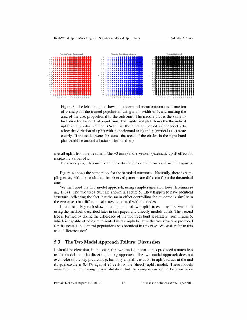
Figure 3: The left-hand plot shows the theoretical mean outcome as a functionof x and y for the treated population, using a bin-width of 5, and making thearea of the disc proportional to the outcome. The middle plot is the same il-lustration for the control population. The right-hand plot shows the theoreticaluplift in a similar manner. (Note that the plots are scaled independently toallow the variation of uplift with x (horizontal axis) and y (vertical axis) moreclearly. If the scales were the same, the areas of the circles in the right-handplot would be around a factor of ten smaller.)

overall uplift from the treatment (the +3 term) and a weaker systematic uplift effect forincreasing values of y.

The underlying relationship that the data samples is therefore as shown in Figure 3.

Figure 4 shows the same plots for the sampled outcomes. Naturally, there is sam-pling error, with the result that the observed patterns are different from the theoreticalones.

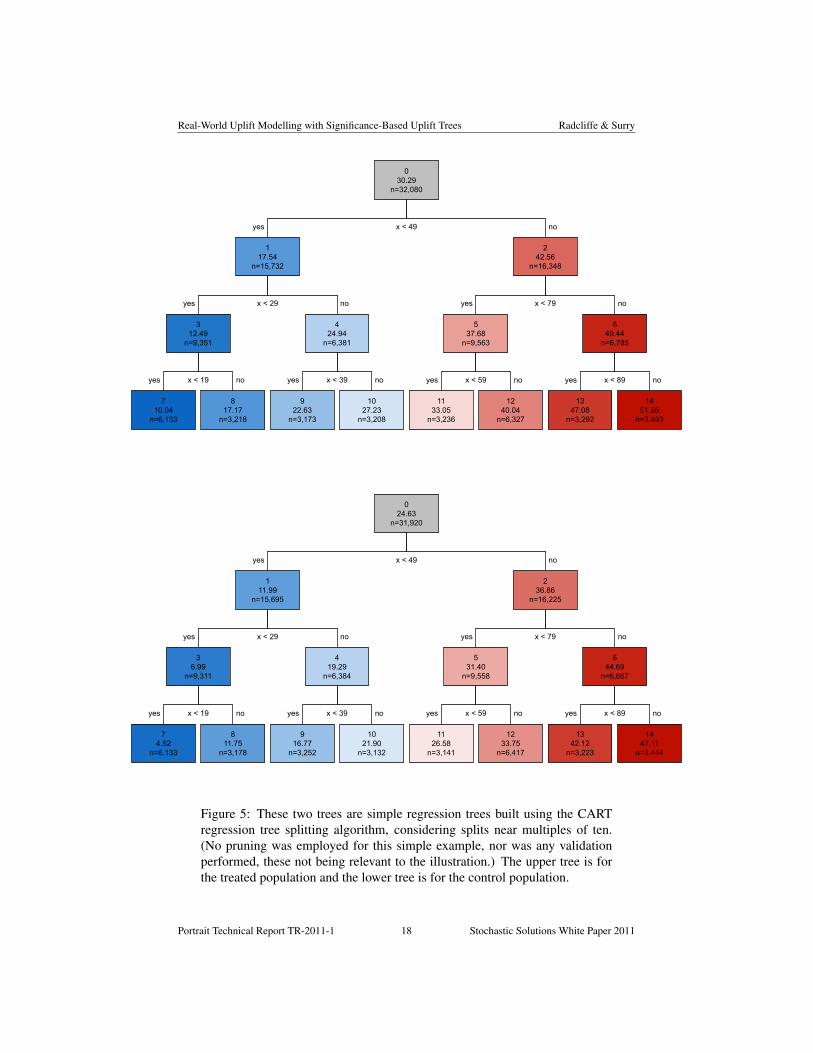
We then used the two-model approach, using simple regression trees (Breiman etal., 1984). The two trees built are shown in Figure 5. They happen to have identicalstructure (reflecting the fact that the main effect controlling the outcome is similar inthe two cases) but different estimates associated with the nodes.

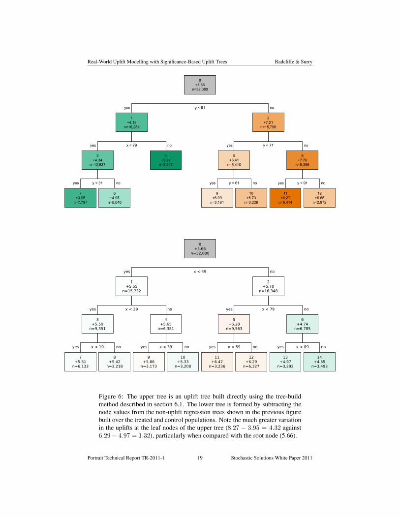
In contrast, Figure 6 shows a comparison of two uplift trees. The first was builtusing the methods described later in this paper, and directly models uplift. The secondtree is formed by taking the difference of the two trees built separately, from Figure 5,which is capable of being represented very simply because the tree structure producedfor the treated and control populations was identical in this case. We shall refer to thisas a ‘difference tree’.

5.3 The Two Model Approach Failure: DiscussionIt should be clear that, in this case, the two-model approach has produced a much lessuseful model than the direct modelling approach. The two-model approach does noteven refer to the key predictor, y, has only a small variation in uplift values at the andits q0 measure is 8.44% against 25.72% for the (direct) uplift model. These modelswere built without using cross-validation, but the comparison would be even more



Actual Treated Outcomes by x & y

<= 4

5 - 9

10 - 14

15 - 19

20 - 24

25 - 29

30 - 34

35 - 39

40 - 44

45 - 49

50 - 54

55 - 59

60 - 64

65 - 69

70 - 74

75 - 79

80 - 84

85 - 89

90 - 94

>= 95

<= 4

5 - 9

10 - 14

15 - 19

20 - 24

25 - 29

30 - 34

35 - 39

40 - 44

45 - 49

50 - 54

55 - 59

60 - 64

65 - 69

70 - 74

75 - 79

80 - 84

85 - 89

90 - 94

>= 95

x

y

Actual Control Outcomes by x & y

<= 4

5 - 9

10 - 14

15 - 19

20 - 24

25 - 29

30 - 34

35 - 39

40 - 44

45 - 49

50 - 54

55 - 59

60 - 64

65 - 69

70 - 74

75 - 79

80 - 84

85 - 89

90 - 94

>= 95

<= 4

5 - 9

10 - 14

15 - 19

20 - 24

25 - 29

30 - 34

35 - 39

40 - 44

45 - 49

50 - 54

55 - 59

60 - 64

65 - 69

70 - 74

75 - 79

80 - 84

85 - 89

90 - 94

>= 95

x

y

Actual Uplift by x & y

<= 4

5 - 9

10 - 14

15 - 19

20 - 24

25 - 29

30 - 34

35 - 39

40 - 44

45 - 49

50 - 54

55 - 59

60 - 64

65 - 69

70 - 74

75 - 79

80 - 84

85 - 89

90 - 94

95

<= 4

5 - 9

10 - 14

15 - 19

20 - 24

25 - 29

30 - 34

35 - 39

40 - 44

45 - 49

50 - 54

55 - 59

60 - 64

65 - 69

70 - 74

75 - 79

80 - 84

85 - 89

90 - 94

95

X

Y

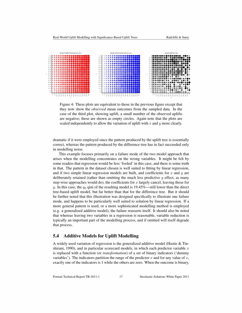
Figure 4: These plots are equivalent to those in the previous figure except thatthey now show the observed mean outcomes from the sampled data. In thecase of the third plot, showing uplift, a small number of the observed upliftsare negative; these are shown as empty circles. Again note that the plots arescaled independently to allow the variation of uplift with x and y more clearly.

dramatic if it were employed since the pattern produced by the uplift tree is essentiallycorrect, whereas the pattern produced by the difference tree has in fact succeeded onlyin modelling noise.

This example focuses primarily on a failure mode of the two model approach thatarises when the modelling concentrates on the wrong variables. It might be felt bysome readers that regression would be less ‘fooled’ in this case, and there is some truthin that. The pattern in the dataset chosen is well suited to fitting by linear regression,and if two simple linear regression models are built, and coefficients for x and y aredeliberately retained (rather than omitting the much less predictive y effect, as manystep-wise approaches would do), the coefficients for x largely cancel, leaving those fory. In this case, the q0 qini of the resulting model is 19.45%—still lower than the directtree-based uplift model, but far better than that for the difference tree. But it shouldbe further noted that this illustration was designed specifically to illustrate one failuremode, and happens to be particularly well suited to solution by linear regression. If amore general pattern is used, or a more sophisticated modelling method is employed(e.g. a generalized additive model), the failure reasserts itself. It should also be notedthat whereas leaving two variables in a regression is reasonable, variable reduction istypically an important part of the modelling process, and if omitted will itself degradethat process.

5.4 Additive Models for Uplift ModellingA widely used variation of regression is the generalized additive model (Hastie & Tin-shirani, 1990), and in particular scorecard models, in which each predictor variable xis replaced with a function (or transformation) of a set of binary indicators (‘dummyvariables’). The indicators partition the range of the predictor x and for any value of x,exactly one of the indicators is 1 while the others are zero. When the outcome is binary,



030.29

n=32,080

x < 49yes no

117.54

n=15,732

x < 29yes no

312.49

n=9,351

x < 19yes no

710.04

n=6,133

817.17

n=3,218

424.94

n=6,381

x < 39yes no

922.63

n=3,173

1027.23

n=3,208

242.56

n=16,348

x < 79yes no

537.68

n=9,563

x < 59yes no

1133.05

n=3,236

1240.04

n=6,327

649.44

n=6,785

x < 89yes no

1347.08

n=3,292

1451.65

n=3,493

024.63

n=31,920

x < 49yes no

111.99

n=15,695

x < 29yes no

36.99

n=9,311

x < 19yes no

74.52

n=6,133

811.75

n=3,178

419.29

n=6,384

x < 39yes no

916.77

n=3,252

1021.90

n=3,132

236.86

n=16,225

x < 79yes no

531.40

n=9,558

x < 59yes no

1126.58

n=3,141

1233.75

n=6,417

644.69

n=6,667

x < 89yes no

1342.12

n=3,223

1447.11

n=3,444

Figure 5: These two trees are simple regression trees built using the CARTregression tree splitting algorithm, considering splits near multiples of ten.(No pruning was employed for this simple example, nor was any validationperformed, these not being relevant to the illustration.) The upper tree is forthe treated population and the lower tree is for the control population.



0+5.66

n=32,080

y < 51yes no

1+4.15

n=16,284

x < 79yes no

3+4.34

n=12,837

y < 31yes no

7+3.95

n=7,797

8+4.95

n=5,040

4+3.24

n=3,447

2+7.21

n=15,796

y < 71yes no

5+6.41

n=6,410

y < 61yes no

9+6.09

n=3,181

10+6.73

n=3,229

6+7.76

n=9,386

y < 91yes no

11+8.27

n=6,414

12+6.65

n=2,972

0+5.66

n=32,080

x < 49yes no

1+5.55

n=15,732

x < 29yes no

3+5.50

n=9,351

x < 19yes no

7+5.51

n=6,133

8+5.42

n=3,218

4+5.65

n=6,381

x < 39yes no

9+5.86

n=3,173

10+5.33

n=3,208

2+5.70

n=16,348

x < 79yes no

5+6.28

n=9,563

x < 59yes no

11+6.47

n=3,236

12+6.29

n=6,327

6+4.74

n=6,785

x < 89yes no

13+4.97

n=3,292

14+4.55

n=3,493

Figure 6: The upper tree is an uplift tree built directly using the tree-buildmethod described in section 6.1. The lower tree is formed by subtracting thenode values from the non-uplift regression trees shown in the previous figurebuilt over the treated and control populations. Note the much greater variationin the uplifts at the leaf nodes of the upper tree (8.27 − 3.95 = 4.32 against6.29− 4.97 = 1.32), particularly when compared with the root node (5.66).



a common choice for the transformation is the so-called weight of evidence, defined asthe log of the odds ratio. So the weight of evidence for the ith bin is

wi = ln

(piqi

)(6)

where pi = P (Y = 1|X = i) and qi = 1 − pi. There is also the adjusted weight ofevidence, which simply subtracts off the overall log odds, i.e.

w∗i = ln

(piqi

)− ln

(p

q

)(7)

where p is the overall outcome rate P (Y = 1) and q = 1− p.The transformation can be viewed as a two-level model, in which rather than mod-

elling the outcome directly in terms of the predictor variables, we first build a simplemodel by averaging the outcome over various bins and then fit the linear model in termsof the output from that first model. Larsen (2010) proposes a method of uplift mod-elling based on adapting this approach to use a ‘net’ version of the adjusted weight ofevidence:19

∆w∗i = w∗i,T − w∗i,C . (8)

The use of a net weight of evidence is helpful, but still leaves the question of how toperform the regression itself. Larsen’s approach is similar to the method of Lo (2002),in that he performs a logistic regression (using the net adjusted weight of evidencetransformation) with separate parameters for the treated and control cases.

Although we have not tried this method ourselves, it seems plausible that the com-bination of Lo’s basic method with the added benefit of the net adjusted weight ofevidence transformation could work well.

6 The Significance-Based Uplift TreeWhen modelling uplift directly (with a single model) the core problem is that outcomescannot be measured at the level of the individual. This has implications for the fittingprocess itself and for measuring model quality. Given the absence of individual out-comes, we use estimated outcomes for segments (subpopulations).

A natural class of models to consider is tree-based models, since these are intrinsi-cally based on segments; these are introduced in section 6.1 and extended to continuousoutcomes in 6.3. (Regression methods based on binned variable transformations are an-other promising candidate, since the transformation can group values from a segment,as discussed earlier in section 5.4).

We now describe the approach to uplift modelling currently favoured by the au-thors, which forms the core of the uplift modelling available in the Portrait Upliftproduct from Pitney Bowes. The key features of the current approach are:

• the signficance-based splitting criterion (section 6.2).19Larsen refers simply to the weight of evidence, but his formulae make it clear that it is the adjusted

version that he uses.



• variance-based pruning (section 6.5);

• use of bagging (section 6.6);

• pessimistic qini-based variable selection (section 7.4).

The significance-based pruning criterion was introduced to the software (but no algo-rithmic details were published) in 2002; the other features were added between 2002and 2007.

6.1 Tree-based Uplift ModellingThe criteria used for choosing each split during the growth phase of standard divisivebinary tree-based methods (notably CART and Quinlan’s various methods) trade offtwo desirable properties:

• maximization of the difference in outcome between the two subpopulations;

• minimization of the difference in size between them.

These tend to be inherently in conflict, as it is usually easy to find small populations thatexhibit extreme outcome rates—for example, splitting off one purchaser (a segmentwith a 100% purchase rate) from the main population.

We approach split conditions for uplift trees from the same perspective, the dif-ference being that the outcome is now the uplift in each subpopulation, rather than asimple purchase rate or similar.

The method of Hansotia & Rukstales (2001) is simply the result of ignoring thetrade-off and directly using the difference in uplifts (which they call “∆∆p”) as thesplit criterion. Notwithstanding their reported success, we have not had good resultswith this approach.

We have also tried using qini directly as the split quality measure. Qini does takeinto account both population size and uplift on each side of the split, but although wefind qini useful for assessing the overall performance of uplift models, we have hadonly limited success in using it as a split criterion. The fact that qini only measuresrank ordering is probably a factor here.

It is also possible to take an ad hoc approach, whereby the difference in populationsizes is treated as some sort of penalty term to adjust the raw difference in uplifts. Ifthe (absolute) difference in uplifts is ∆ and the two subpopulation sizes are NL andNR, a natural candidate penalized form might be

∆ /

(NL +NR

2 min(NL, NR)

)k

, (9)

for some k. This penalty is 1 when the populations are even and increases as theybecome more uneven. Another obvious alternative penalized form might be

∆

(1−

∣∣∣∣NL −NR

NL +NR

∣∣∣∣k)

(10)



for some k. Here, the penalty is zero for equal-sized populations and increases to 1 astheir sizes diverge. (In both cases, k, is a parameter to be set heuristically.) Our earliestmethod, described in Radcliffe & Surry (1999), was of this general form. However, wefailed to find any ad hoc penalty scheme that worked well across any useful range ofreal-world problems.

6.2 The Significance-Based Splitting CriterionOur current significance-based splitting criterion fits a linear model to each candidatesplit and uses the significance of the interaction term as a measure of the split quality.Considering first the case of a binary outcome we model the response probability as

pij = µ+ αi + βj + γij (11)

where

• p is the response probability;

• i is T for a treated customer and C for a control;

• j indicates the side of the split (L or R);

• µ is a constant related to the mean outcome rate;

• α quantifies the overall effect of treatment;

• β quantifies the overall effect of the split;

• the interaction term, γ, captures the relationship between the treatment and thesplit.

Without loss of generality, we can set

αC = βL = γCL = γCR = γTL = 0. (12)

Then, γTR is the difference in uplift between the two subpopulations, which is exactlythe quantity in which we are interested.

For a given dataset with known (binary) outcomes and values for the candidatesplit, we can determine γTR and its significance by fitting the linear model definedby equations 11 and 12 using standard weighted (multiple) linear regression. We thenuse the significance of γTR as the quality measure for the split. The significance ofparameters in a multiple linear regression is given by a t-statistic (Jennings, 2004).Note that the relevant t-statistic tests the significance of the estimator for γTR giventhat the other variables are already in the model, thus isolating the effect of the spliton uplift, which is what we are interested in.

In practice, since we do not care about which side of the split is higher, it sufficesto maximize the square of the statistic

t2{γTR} =γ2TR

s2{γTR}(13)



where our parameter γTR is estimated using the observed difference in uplift betweenthe left and right populations, UR − UL ≡ (pTR − pCR)− (pTL − pCL), and

s2{γTR} = MSE × C44, (14)

whereMSE is the mean squared error from the regression andC44 is the (4,4)-elementof C = (X′X)−1. Here, X is the design matrix for the regression

X =

1 X11 X12 X13

1 X21 X22 X23

......

......

1 Xn1 Xn2 Xn3

, (15)

in which Xi1 indicates whether the ith record was treated, Xi2 indicates whether theith record was on the right of the split, and Xi3 = Xi1Xi2 is the interaction indicator,set to 1 when the record is treated and on the right of the split. We have four degreesof freedom in the regression (corresponding to µ, αT , βR and γTR) so the MSE =SSE/(n− 4) where n is the number of observations.

Simplifying C, we find that

C44 =1

NTR+

1

NTL+

1

NCR+

1

NCL, (16)

the reciprocal harmonic mean of the cell sizes, Nij . In practice, therefore, the expres-sion we actually use for split quality is

t2{γTR} =(n− 4)(UR − UL)2

C44 × SSE, (17)

withSSE =

∑i∈{T,C}

∑j∈{L,R}

Nijpij(1− pij). (18)

6.3 Continuous or Ordered OutcomesUp to this point, we have focused on cases in which the outcome that we wish tomodel is binary, but there are also common cases in which the outcome is continuous.20

Perhaps the most common case is a campaign where the goal is to increase customerspend, so that the uplift in question is the incremental spend attributable to the treatment(equation 4).

The significance-based split criterion defined by equations 11 and 13 is based onfitting a linear model, so can be extended to the continuous case without modification,i.e. the pij in equation 11 can now be replaced with a general outcome Oij . The calcu-lation of the SSE in equation 18 becomes slightly more complicated, but the formulaeare otherwise unchanged.

NOTE: In classical response modelling, if the “response” rate is low, it is common20or more generally, an ordered outcome, which can include a discrete ordinal.



practice to adopt a two-stage approach to estimating outcomes by expressing the ex-pected revenue R as

E(R) = P (R > 0) · E(R |R > 0). (19)

This would then be modelled using a binary model for the first term and weightedby a continuous model built only on people in the training data with non-zero spend.This approach is used because a large number of zeros can often limit the ability of acontinuous model to fit the non-zero values accurately.

Similarly, modelling uplift in spend directly with a single uplift model is best suitedto situations in which the outcome for most people is a non-zero spend.

If most people will not, in fact, spend, it may well be that a two stage approach,with a binary uplift model and a conventional continuous model over the spenders willbe a more effective approach. The continuous model, in this case, should be built onthe purchasers in the treated population, rather than the whole population.

6.4 Multiplicative Uplift and ModellingThe authors have a strong bias towards modelling uplift as an additive phenomenon, i.e.towards measuring uplift as an absolute difference between mean outcomes in treatedand control populations. An alternative approach would be to measure uplift multi-plicatively, i.e. to use the ratio of the outcomes in the treated and control populations.We have developed, but never use, a version of the significance-based uplift tree forsuch multiplicative uplift, and we have chosen not to document it here.

The reason we favour measuring uplift as a difference is we have been unable tofind any plausible application in which it would be rational to act based on the ratio ofoutcomes rather than the difference.

For example, consider a marketing application in which there is a choice of target-ing segment A, in which our treatment increases response rate from 1% to 1.5%, orsegment B, in which the response rate is raised from 5% to 6%. Other things beingequal (including the segment sizes), the value of targeting segment B is twice that oftargeting segment A, even though the uplift ratio in segment A is 50% compared withonly 20% in segment B. Money is additive.

From a utilitarian perspective, the same is true with medical interventions: even ifa drug completely cures all patients of type A, with an untreated mortality rate of 1%,and “only” reduces mortality from 90% to 30% is segment B, it is clear that targetingpatients in segment B reduces mortality 60 times more than does targeting segment A,notwithstanding the infinite uplift ratio in segment A.

This seems to be the invariable pattern, at least when the true outcome is beingmeasured.

It might, in principle still be preferable to model uplift as a ratio if the underlyingimpact of the treatment were believed to be multiplicative, because in such cases itseems likely that a more accurate model would result. In practice, however, to under-stand the (additive) impact of action, it would still be necessary to model the outcomewithout treatment and then to compute the uplift as a difference, leading to similarproblems to those identified with the two model approach earlier. We do not, therefore,recommend using a definition of uplift as a ratio.



6.5 Variance-Based Pruning and Limiting Split ChoicesMost classical decision tree algorithms involve first building a deep tree by recursivesplitting and then pruning the resulting bushy tree by removing unhelpful splits. Forexample, both CART and Quinlan’s algorithms use this approach. The pruning phaseis intended to reduce overfitting and commonly uses some form of cross-validation.

The main reason for adopting such a two-stage approach is that trees are highlynon-linear models in which predictions can depend strongly on the interaction betweenvariables. Where there are strong non-linear patterns in the data, it may be that anenabling split higher up a tree is only marginally useful by itself, but becomes moreuseful lower down when combined with a further split, so true value of a split cannotalways be determined without further splitting.

In the most extreme form of the growth algorithm, splitting continues until all nodesare pure (i.e. have identical outcomes for all records) or no further useful splits can befound that increase purity. It is common practice, however, when working with largedatasets to limit the smallest population size allowable, and possibly also the maximumdepth of the tree. It is also common to consider only a subset of possible splits, ratherthan literally every possible univariate split, as is recommended in CART (Breiman etal., 1984).

All of these points apply if anything more strongly in the case of typical upliftmodels. The challenges with uplift modelling include (1) overall uplift is often smallcompared to the background effect (2) the control population is commonly smallerthan the treated population, often by a factor of ten or more (3) uplift is a second-orderphenomenon, with consequently large errors associated with the estimates. For all ofthese reasons, the single biggest challenge with uplift modelling tends to be producingstable models in the face of these difficulties.

The approach to pruning we have found most successful for significance-baseduplift trees involves resampling the training population (with replacement) k times; weusually take k=8. Numbering the resulting resampled populations 1–k, we train onpopulation 1 and then evaluate the stability of the tree with reference to populations2–k. We measure the uplift in population 1 at each node, and then estimate its standarddeviation across the remaining seven populations. Splits (and their descendents) areremoved if the uplift at either child node exhibits a standard deviation greater thansome pre-determined threshold. The exact details are not important except to notethat it is the deviation from the mean in population 1 that we measure, because that isthe uplift estimate that the tree will use. It is hard to generalize, because it varies somuch from dataset to dataset, but for typical marketing problems, where backgroundrates might be 1–3% and uplift might be 0.1 to 2 percentage points, we most often usepruning thresholds in the range 0.5% to 3%.

It should be emphasized that resampling and pruning all happens within a trainingpopulation; any population held back for validation of the final model is not involved.

6.6 Bagging for StabilityIn practice, once a sensible approach to modelling and variable selection has been iden-tified, the main practical difficulty encountered when building uplift models is achiev-



ing model stability. The difficulty arises from the combination of trying to model asecond-order phenomenon and the typically low strength of the interaction relative tothe background effect. In plainer words, uplift modelling is particularly hard in prac-tice because it is often applied to situations in which the overall impact being modelledis modest.

In addition to using pessimistic qini estimates in the variable selection, we tendto employ a number of other mechanisms for increasing robustness, including, mostimportantly, bagging (Breiman, 1997). As with variable selection, we most commonlyform n = 8 populations by resampling the training set (with replacement). We thenbuild a model on one of the populations and validate it on the other partitions, reject-ing the model if it fails to validate appropriately. We build a number of such models(typically b = 10 or 20), each using different resamplings, and average their predic-tions. Employing this approach, we often succeed on problems that we cannot modeleffectively using a single tree. This approach is related to, though different from, therandom forests approach suggested by Breiman (2001).

7 Variable SelectionVariable selection is recognized as an important part of any model-building process.Our experience is that it is actually of greater importance in uplift modelling than inconventional modelling.

7.1 Conventional Motivations for Variable SelectionIn the context of conventional modelling, there are a number of different motivationsfor reducing the set of variables prior to model building, depending on the type ofmodel being built, the build method and the purpose to which the model is to be put.Some of the more important motivations include:

1. Reducing the dimensionality of the model and the likelihood of overfitting. Formodelling approaches in which all available variables are used (such as tradi-tional multiple regression), there is a clear need to reduce the number of variables(if large) to control the number of degrees of freedom. Performing a regressionwith a large number of independent parameters will tend to result in severe over-fitting.21

2. Avoiding correlation. There are a number of difficulties with using strongly cor-related variables in modelling, particularly if the model is supposed to be causal.If a pair of strongly correlated variables exists, there is generally freedom toincrease the weight on one and decrease the weight on the other, leading, at aminimum, to interpretational challenges, and in practice often to unstable resultsand numerical errors.

21Transformations, as discussed in section 5.4 are also, among other things, a way of reducing the numberof degrees of freedom.



3. Improving model quality and stability. For some build methods, removing vari-ables can actually improve model quality even on the training data. As a simpleexample of the principle, standard greedy tree-building methods do not, in gen-eral, produce optimal trees, and it can be the case that removing a variable thatwill be used for splitting at one level will actually result in a better tree whenmore levels are built.

Validation considerations increase this motivation. In almost all models, it is bet-ter to remove a variable that will cause instability before the model build properthan to leave it in. If (ultimately) left in, it will normally degrade the model.If taken out at some later stage, its damage will often have been done, eitherby leaving other model parameters set suboptimally, or by having effectively re-moved the chance for better variables to be included in the model. For example,in the standard tree-building approach the tree is first built (greedily) on a train-ing population, and then pruned using a validation population. There is no “tryre-building with alternative variables” phase, so splits removed during pruninghave prevented other splits, that might not have been pruned, from appearing inthe tree.

4. Improving model interpretability. When models are to be interpreted, differentvariables may lead to different interpretations. Moreover, given a pair of corre-lated variables, x1 and x2, both useful as predictors of the outcome, o, it maybe, for example, that x1 actually drives x2 and o; in this case, there is a strongadvantage in using x1 rather than x2 as the predictor, particularly if other factorsdrive x2, but not o, so that in future x1 might remain a better predictor if x1 andx2 diverge.

7.2 Motivations for Variable Selection in Uplift ModellingIn the context of uplift modelling, while all of these considerations remain, our ex-perience suggests that motivation 3 comes to the fore. This is because uplift mod-els are second-order models in the sense that they model the difference between twooutcomes, rather than a direct outcome. Because of this, and also because in manypractical cases the uplift is small relative to the direct outcomes, the risk of overfittingincreases markedly.

Indeed, we could state this more strongly. Before we developed suitable variableselection procedures for uplift modelling, it was common for our uplift models to fail tovalidate to any useful degree (or to be pruned right back to the root during the pruningphase). In this sense, we have found that for many practical problems, good variableselection is an absolute prerequisite for uplift modelling.

7.3 Desirable Properties of Variable Selection MethodsGiven the above, there are three main attributes we might seek from the predictorschosen by a variable-selection procedure for uplift modelling:

1. predictiveness;



2. stability (robustness);

3. independence.

The first is fundamental: if we don’t have variables that are predictive, by definitionwe have little hope of building a useful model.

We believe that the second, as discussed above, is even more important for upliftmodels than for conventional models, because the risk of instability (in the sense offailure to validate) is that much higher for second-order models.

The third, though desirable, is probably less important, particularly when usingtree-based methods. Other things being equal, it is certainly better to identify a setof candidate predictors that capture different aspects of the relationship and thus havelow correlation. To some extent, step-wise methods for regression seek to achieve this.In practice, however, we find that if we are effective in removing variables that leadto instability, and in including primarily variables with good correlation, our trees areusually quite effective at combining them to produce useful uplift models.

7.4 Pessimistic Qini EstimatesThe simplest approach to variable selection is to use a quality measure to rank thecandidate variables and then to take the best ones identified, usually either choosing afixed number, or all those above some threshold, perhaps again subject to a thresholdquality.

We have had success using this approach with quality measures based on qini.However, in light of the need for stability/robustness, as highlighted above, we havefound it useful to modify our qini estimates to be more pessimistic, thereby furtherreducing the likelihood of choosing variables that will lead to unstable models.

There are various ways if making such a pessimistic, or ‘low’ qini estimate (LQE).Our approaches are mostly based on subtracting some kind of estimate of the spreadof the qini distribution. To do this, we most often resample the training population ina manner similar to that used with bagging (Breiman, 1997). Thus, in our currentlyfavoured approach, we produce n different resampled variants of the population (typi-cally n = 8), all of which have the same size as the original and which are formed byresampling the training population with replacement. We then calculate the qini22 ineach population to form a set of estimates q̂1, q̂2, . . . , q̂n. We then adjust the qini esti-mate by subtracting off some multiple of s, the sample standard deviation. While themost natural multiple to take off is probably something like 1/

√n (' 0.35 for n = 8),

we tend to use a larger multiple than this, often in the range 0.5 to 1.0, and to someextent use this factor as a control parameter for the variable selection. Most often, westart with it at 0.5, then increase it if we find we are having problems with model sta-bility and reduce it if we find stability is acceptable and we are seeking to increase thepredictive power of the model.

Many variations on this basic theme are possible.

22usually using the unscaled qini, Q, to avoid problems should the overall uplift be zero



7.5 Net Information ValueAs noted above, Larsen (2010) has proposed the net information value as a method forvariable selection for uplift modelling with binary outcomes.

The (ordinary) information value (I) is formed from the adjusted weight of evi-dence w∗i by forming a weighted sum of the weights of evidence over the bins, weight-ing each weight of evidence by the difference in outcome rates (1 and 0) in the bin,i.e.

I =∑i

w∗i (P (O = 1|X = i)− P (O = 1|X = i)) (20)

This is a common metric used for variable selection in conventional modelling. Larsenproposes a modification of this using his net weight of evidence and the four likelihoodsassociated with each bin (outcomes 1 and 0 for treated and control).

Larsen defines net information value IN as essentially∑i

∆w∗i

(P (X = i|O = 1)TP (X = i|O = 0)C

−P (X = i|O = 0)TP (X = i|O = 1)C

). (21)

We have not experimented with this approach.

8 Closing RemarksThe authors have been using uplift modelling commercially in various forms for sometwelve years now, and have been surprised that use of the approach has grown as slowlyas it has. However, the use of uplift modelling, in various forms, is now on the rise. Wehope this more detailed paper discussing the techniques will encourage that continuedgrowth, since, from the authors’ perspective, it is now clearly demonstrated not onlythat uplift modelling is the correct formulation of the problem that many marketersare trying to solve, but also that the techniques presented here and elsewhere can, inmany cases, produce measurable results that are variously superior in terms of prof-itability, cost and targeting volume, while reducing negative effects. We will close bydiscussing what we have learned, heuristically, about when uplift modelling is moreand less effective relative to the alternatives.

8.1 When is Uplift Modelling Worthwhile?While we would argue that, in principle, uplift modelling is almost always, from atheoretical perspective, the correct way to formulate marketing response modelling, itis not the case that in practice, it will always produce superior results, nor that evenwhen it will, the improvement always justifies the extra complexity. We suggest thefollowing checklist when deciding whether or not to take an uplift modelling approach.

• Existence of a valid control group. Straightforwardly, if no valid control groupexists in the historical data, uplift modelling cannot normally be employed. (Butone can be created for the next iteration of the campaign.)



• Volume. Not only must a control group exist, but it must be large enough to sup-port uplift modelling. One rule of thumb we use is that the control group23 needsto be at least ten times larger for modelling than it does for simple measurementof incremental response. A second rule of thumb is that, for modelling binaryoutcomes, the product of the overall uplift and the size of each population shouldbe at least 500. So, if the overall uplift is 0.1%, this means that both the treatedand the control group need to be at least 500,000.

• Negative Effects. The likely (or known) presence of negative effects is a strongreason to consider uplift modelling seriously. Conventional modelling is inher-ently unable to handle negative effects, and negative effects are doubly harmful,in that they both carry a cost of action and reduce the overall impact of the activ-ity. It is not uncommon, particularly in the area of retention, for uplift modellingto deliver more value by identifying populations where negative effects are preva-lent than from ranking the parts of the population where the impact is neutral orpositive. Negative effects tend to occur most when uplift is small relative to thebackground outcome rate, where inaction on the part of the customer leads to apositive outcome for the supplier, where interventions are intrusive, and wherecustomers targeted are already unhappy with the supplier, which is why upliftmodelling has been perhaps most widely used and most effective in customerretention applications.

• Complex Customer Influences. Where the customer is subject to many influ-ences (advertising, multiple communications, in-branch activity etc.), the riskof attributing sales incorrectly to a particular piece of marketing activity is largerthan where there are fewer interventions, so the difference between uplift modelsand conventional models tends to be more marked.

• Anticorrelated Outcomes. A situation we commonly see in retail environmentsis that direct marketing activity appears to have the most positive effect on high-spending customers. Where this is the case, uplift and sales are positively cor-related, and therefore a conventional model and an uplift model are more likelyto rank the population in similar ways. While we first conceived uplift mod-elling in a retail sales context, and have had some positive results in this area,overall we have found the benefits of uplift modelling are often smaller in retailenvironments, where we often see these positive correlations, than in some otherareas.

Conversely, almost by definition, when the (non-incremental) outcome is anticor-related with the incremental impact of marketing activity, a conventional modelis likely to perform particularly badly, and the benefit of uplift modelling may belarger. This is the case when, for example, a marketing offer succeeds in drivingup purchase rate most among a group of customers who normally do purchaselittle, but where that group remains a relatively low purchasing group. The twocases are illustrated in figure 7.

23Technically, the smaller of the control group and the treated group, but usually this is the control group



Correlated Uplift and Outcome

Out

com

e an

d U

plift

Target deciles, worst to best

Treated

Control

Uplift

Anticorrelated Uplift and Outcome

Out

com

e an

d U

plift

Target deciles, worst to best

Treated

Control

Uplift

Figure 7: The graph on the left illustrates positive correlation between out-come (top two lines) and uplift (bottom line). A conventional model built oneither population should rank this population well for uplift. The graph on theright illustrates negative correlation between outcome (ascending lines) anduplift (descending line). A conventional model built on either population willtend to rank the worst group by uplift as the best targets.

• Background Rate and Brand Recognition. Another situation in which conven-tional analysis may well be misled is when the background outcome rate is high.As an extreme example, sending an incentive to an existing regular weekly cus-tomer and then counting a purchase the following week as a ‘response’ is prob-ably unwise. On the other hand, a little known brand that targets people whoare unlikely to have heard of the company or product might reasonably be moreconfident that apparent responses really are incremental even without a controlgroup, and in such cases, an uplift model may offer little or no benefit, or mayactually perform worse than a conventional ‘response’ model.

8.2 The Trade OffUltimately, with uplift modelling, there is a trade-off between modelling the right thing(which uplift modelling, applied appropriately, does) against the added complexity ofmodelling and increased data requirements that are inherent in the second-order prob-lem formulation that uplift modelling involves. We have tried to give guidance aboveas to when that trade-off genuinely favours the uplift approach and when it may fail todeliver value. We close with the wise and germane words of Tukey (1962):

Far better an approximate answer to the right question . . . than the exactanswer to the wrong question.24

24The full quote is “Far better an approximate answer to the right question, which is often vague, than theexact answer to the wrong question, which can always be made precise.” In our case, there is nothing vagueabout the right question, but it is the case that, as second-order models, uplift models usually have largererror bars than conventional models, and are in this sense “more approximate”.



AcknowledgementsMany people contributed to the development of uplift modelling over a period thatspanned more than a decade. We would like to recognize and thank, in particular,David Signorini and Tim Harding, as well as Ian Bradbury, Ann Gould, Elaine Farrow,Bob Fletcher, Sandy Nicholson, Rob Simpson, Brian Gibb, Ian Flockhart and otherstoo numerous to list, all of whom contributed to the ideas, implementation, testing andother aspects of the research programme that resulted in uplift modelling as it is today.

ReferencesL. Breiman, J. Freidman, R.A.Olshen, and C. Stone, 1984. Classification and Regression Trees.

Wadsworth.

L. Breiman, 1997. Arcing classifiers. Technical report, Statistics Department, University ofCalifornia at Berkley.

L. Breiman, 2001. Random forests. Machine Learning.

D. M. Chickering and D. Heckerman, 2000. A decision-theoretic approach to targeted advertis-ing. In Sixteenth Annual Conference on Uncertainty in Artificial Intelligence, Stanford, CA.

T. H. Cormen, C. E. Leiserson, and R. L. Rivest, 1990. Chapter 16, greedy algorithms. InIntroduction to Algorithms, page 329. MIT Press and McGraw-Hill.

D. Durand, 1941. Risk elements in consumer instalment financing. Technical report, NationalBureau of Economic Research, New York.

M. D. Grundhoefer, 2009. Raising the bar in cross-sell marketing with uplift modeling. InE. Siegel, editor, Predictive Analytics World Conference, Washington, D.C. Prediction ImpactInc.

D. J. Hand and K. Yu, 2001. Idiot’s Bayes — not so stupid after all? International StatisticalReview, 69:385–399.

D. J. Hand, 1981. Discrimination and Classification. John Wiley (Chichester).

B. Hansotia and B. Rukstales, 2001. Incremental value modeling. In DMA Research CouncilJournal, pages 1–11.

B. Hansotia and B. Rukstales, 2002. Direct marketing for multichannel retailers: Issues, chal-lenges and solutions. Journal of Database Marketing, 9(3):259–266.

T. J. Hastie and R. J. Tibshirani, 1990. Generalized Additive Models. Chapman & Hall.

D. M. Hawkins and G. Kass, 1982. Automatic interaction detection. In D. Hawkins, editor, Topicsin Applied Multivariate Analysis, pages 269–302. Cambridge University Press (Cambridge).

K. Hillstrom, 2008. The minethatdata e-mail analytics and data mining challenge. http://blog.minethatdata.com/2008/03/minethatdata-e-mail-analytics-and-data.html.

K. Jennings, 2004. Statistics 512: Applied linear models, topic 3, chapter 5. Technical report,Perdue University.

G. V. Kass, 1980. An exploratory technique for investigating large quantities of categorical data.Applied Statistics, 29(2):119–127.

K. Larsen, 2010. Net lift models.

V. S. Y. Lo, 2002. The true lift model. ACM SIGKDD Explorations Newsletter, 4(2):78–86.



V. S. Y. Lo., 2005. Marketing data mining – new opportunities. In J. Wang, editor, Encyclopediaof Data Warehousing and Mining. Idea Reference Group.

S. J. Louis and G. J. E. Rawlins, 1993. Pareto optimality, GA-easiness and deception. In S. For-rest, editor, Proceedings of the Fifth International Conference on Genetic Algorithms. MorganKaufmann (San Mateo, CA).

C. Manahan, 2005. A proportional hazards approach to campaign list selection. In SAS UserGroup International (SUGI) 30 Proceedings.

G. Moore, 1991. Crossing the Chasm: Marketing and Selling Technology Products to Main-stream Customers. Harper Business Essentials.

C. T. Onions, editor, 1973. The Shorter Oxford English Dictionary. Clarendon Press (Oxford).

G. Piatetsky-Shapiro, 1991. Discovery, analysis, and presentation of strong rules. In G. Piatetsky-Shapiro and W. J. Frawley, editors, Knowledge Discovery in Databases. AAAI/MIT Press(Cambridge, MA).

J. R. Quinlan, 1986. Induction of decision trees. Machine Learning, 1(1):81–106.

J. R. Quinlan, 1993. C4.5: Programs for Machine Learning. Morgan Kaufmann (San Mateo,CA).

N. J. Radcliffe and R. Simpson, 2008. Identifying who can be saved and who will be drivenaway by retention activity. Journal of Telecommunications Management. Henry Stewart Pub-lications, (to appear).

N. J. Radcliffe and P. D. Surry, 1999. Differential response analysis: Modeling true response byisolating the effect of a single action. In Proceedings of Credit Scoring and Credit Control VI.Credit Research Centre, University of Edinburgh Management School.

N. J. Radcliffe, 2007. Using control groups to target on predicted lift: Building and assessinguplift model. Direct Marketing Analytics Journal, An Annual Publication from the DirectMarketing Association Analytics Council, pages 14–21.

N. J. Radcliffe, 2008. Hillstrom’s MineThatData email analytics challenge: An approachusing uplift modelling. Technical report, Stochastic Solutions Limited. Available fromhttp://stochasticsolutions.com/pdf/HillstromChallenge.pdf.

P. Resnick, N. Iacovou, , M. Suchak, P. Bergstrom, and J. Riedl, 1994. Grouplens: An open archi-tecture for collaborative filtering of netnews. In Proceedings of ACM Conference on ComputerSupported Cooperative Work, pages 175–186. Chapel Hill.

P. Rzepakowski and S. Jaroszewicz, 2010. Decision trees for uplift modeling. IEEE Conferenceon Data Mining, pages 441–450.

E. H. Simpson, 1951. The interpretation of interaction in contingency tables. Journal of the RoyalStatistical Society, Series B, 13:238–241.

P. D. Surry and N. J. Radcliffe, 2011. Quality measures for uplift models. submitted to KDD2011.

L. C. Thomas, 2000. A survey of credit and behavioural scoring: forecasting nancial risk oflending to consumers. International Journal of Forecasting, 16(2):149–172.

J. W. Tukey, 1962. The future of data analysis. Annals of Mathematical Statistics, 33(1):1–67.


Documents

Real-World Uplift Modelling with Signiﬁcance-Based Uplift ...stochasticsolutions.com/pdf/sig-based-up-trees.pdf · Real-World Uplift Modelling with Signiﬁcance-Based Uplift Trees