Embed Size (px)
Citation preview
Realized Variance and Market Microstructure Noise
Peter R. Hansena∗, Asger Lundeb
aStanford University, Department of Economics, 579 Serra Mall,
Stanford, CA 94305-6072, USA
bAarhus School of Business, Department of Marketing and Statistics,
Fuglesangs Alle 4, 8210 Aarhus V, Denmark
First version: January 2004. This version: July, 2005
Abstract
We study market microstructure noise in high-frequency data and analyze its implications for the realized variance(RV) under a
general specification for the noise. We show that kernel-based estimators can unearth important characteristics of market microstruc-
ture noise and that a simple kernel-based estimator dominates theRV for the estimation of integrated variance(IV). An empirical
analysis of the Dow Jones Industrial Average stocks revealsthat market microstructure noise is time-dependent and correlated with
increments in the efficient price. This has important implications for volatility estimation based on high-frequency data. Finally, we
apply cointegration techniques to decompose transaction prices and bid-ask quotes into an estimate of the efficient price and noise.
This framework enables us to study the dynamic effects on transaction prices and quotes caused by changes in the efficientprice.
Keywords: Realized Variance; Realized Volatility; Integrated Variance; Market Microstructure Noise; Bias Correction; High-
Frequency Data; Sampling Schemes.
JEL Classification:C10; C22; C80.
∗Corresponding author, email: [email protected]
1

P. R. Hansen and A. Lunde: Realized Variance and MMS Noise
“The great tragedy of Science – the slaying of a beautiful hypothesis by an ugly fact.” Thomas H. Huxley
(1825–1895).
1. Introduction
The presence of market microstructure noise in high-frequency financial data complicates the estimation of financial
volatility and makes standard estimators – such as the realized variance(RV) – unreliable. Thus, from the perspective of
volatility estimation, market microstructure noise is anugly factthat challenges the validity of theoretical results that rely
on the absence of noise. Volatility estimation in the presence of market microstructure noise is currently a very active
area of research. Interestingly, this literature was initiated by an article by Zhou (1996) that was published in this journal
a decade ago, and Zhou’s paper was in many ways 10 years ahead of its time.
The best remedy for market microstructure noise depends on the properties of the noise and the main purpose of
this paper is to unearth the empirical properties of market microstructure noise. We utilize a number of kernel-based
estimators that are well suited for this problem and our empirical analysis of high-frequency stock returns reveals the
following “ugly” facts about market microstructure noise.
1. The noise is correlated with the efficient price.
2. The noise is time-dependent.
3. The noise is quite small in the DJIA stocks.
4. The properties of the noise have changed substantially over time.
These four empirical “facts” are related to one another and have important implications for volatility estimation. The
time-dependence in the noise and the correlation between noise and efficient price arise naturally in some models on
market microstructure effects, including (a generalized version of) the bid-ask model by Roll (1984) (see Hasbrouck
(2004) for a discussion), and models where agents have asymmetric information, such as those by Glosten & Milgrom
(1985) and Easley & O’Hara (1987, 1992). Market microstructure noise has many sources, including the discreteness
of the data, see Harris (1990, 1991), and properties of the trading mechanism, see e.g. Black (1976) and Amihud &
Mendelson (1987). For additional references to this literature, see e.g. O’Hara (1995) and Hasbrouck (2004).
The main contributions of this paper are as follows: First, we characterize how theRV is affected by market mi-
crostructure noise under a general specification for the noise that allows for various forms of stochastic dependencies.
Second, we show that market microstructure noise is time-dependent and correlated with efficient returns. Third, we
consider some existing theoretical results that are based on assumptions about the noise that are too simplistic, and dis-
cuss when such results provide reasonable approximations.For example, our empirical analysis of the 30 DJIA stocks
2
P. R. Hansen and A. Lunde: Realized Variance and MMS Noise
shows that the noise may be ignored when intraday returns aresampled at relatively low frequencies such as 20-minute
sampling. Assuming the noise is of an independent type seemsto be reasonable when intraday returns are sampled
every 15 ticks or so. Fourth, we apply cointegration methodsto decompose transaction prices and bid/ask quotations
into estimates of the efficient price and market microstructure noise. The correlation between these estimated series are
consistent with the volatility signature plots. The cointegration analysis enables us to study how a change in the efficient
price dynamically affects bid, ask, and transaction prices.
The interest for empirical quantities that are based on high-frequency data has surged in recent years. The realized
variance(RV) is a well known quantity that goes back to Merton (1980). Other empirical quantities include the bi-power
variation and multi-power variation that are particularlyuseful for detecting jumps, see Barndorff-Nielsen & Shep-
hard (2003, 2004, 2005a, 2005b), Andersen, Bollerslev & Diebold (2003), Bollerslev, Kretschmer, Pigorsch & Tauchen
(2005), Huang & Tauchen (2004) and Tauchen & Zhou (2004), andthe intraday range-based estimators, see Christensen
& Podolskij (2005). High-frequency based quantities have proven themselves useful for a number of problems. For
example, several authors have applied filtering and smoothing techniques to time series of theRV to obtain time series
for daily volatility, see e.g. Maheu & McCurdy (2002), Barndorff-Nielsen, Nielsen, Shephard & Ysusi (1996), Engle &
Sun (2005), Frijns & Lehnert (2004), Koopman, Jungbacker & Hol (2005), Hansen & Lunde (2005c), Owens & Steiger-
wald (2005). High-frequency based quantities are also useful in the context of forecasting, see Andersen, Bollerslev &
Meddahi (2004), Ghysels, Santa-Clara & Valkanov (2005), and for the evaluation and comparison of volatility models,
see Andersen & Bollerslev (1998), Hansen, Lunde & Nason (2003), and Patton (2005).
TheRV, which is a sum-of-squared intraday returns, yields a perfect estimate of volatility in the ideal situation where
prices are observed continuously and without measurement error, see e.g. Merton (1980). This result suggests that theRV
should be based on intraday returns that are sampled at the highest possible frequency (tick-by-tick data). Unfortunately,
the RV suffers from a well known bias problem that tends to get worseas the sampling frequency of intraday returns
increases, see e.g. Fang (1996), Andreou & Ghysels (2002), Oomen (2002), and Bai, Russell & Tiao (2004). The source
of this bias problem is known as market microstructure noise, and the bias is particularly evident involatility signature
plots, that first appeared in Fang (1996), see also Andersen, Bollerslev, Diebold & Labys (2000b). So there is a trade-off
between bias and variance when choosing the sampling frequency, as discussed in Bandi & Russell (2005) and Zhang,
Mykland & Aıt-Sahalia (2005). This trade-off is the reasonthat theRV is often computed from intraday returns that are
sampled at a moderate frequency, such as 5-minute or 20-minute sampling.
A key insight to the problem of estimating the volatility from high-frequency data comes from its similarity to the
problem of estimating the long-run variance of a stationarytime series. In this literature, it is well known that autocor-
relation necessitates modifications of the usual sum-of-squared estimator. Those of Newey & West (1987) and Andrews
(1991) are examples of such estimators that are robust to autocorrelation. Market microstructure noise induces autocor-
3
P. R. Hansen and A. Lunde: Realized Variance and MMS Noise
relation in the intraday returns and this autocorrelation is the source of theRV’s bias problem. Given this connection
to long-run variance estimation it is not surprising that “pre-whitening” of intraday returns and kernel-based estimators
(including the closely related subsample-based estimators) are found to be useful in the present context. Zhou (1996)
introduced the use of kernel-based estimators and the subsampling idea to deal with market microstructure noise in high
frequency data. Filtering techniques have been used by Ebens (1999), Andersen, Bollerslev, Diebold & Ebens (2001),
and Maheu & McCurdy (2002) (moving average filter) and Bollen& Inder (2002) (autoregressive filter). Kernel-based
estimators were explored in Zhou (1996), Hansen & Lunde (2003), and Barndorff-Nielsen, Hansen, Lunde & Shephard
(2004), and the closely related subsample-based estimators were used in an unpublished paper by Muller (1993), and in
Zhou (1996), Zhang et al. (2005), and Zhang (2005).
The rest of this paper is organized as follows. In Section 2 wedescribe our theoretical framework and discuss
sampling schemes in calendar time and tick time. We also characterize the bias of theRV under a general specification
for the noise. In Section 3, we consider the case with independent market microstructure noise, which is used in several
papers, including Corsi, Zumbach, Muller & Dacorogna (2001), Curci & Corsi (2004), Bandi & Russell (2005), and
Zhang et al. (2005). We consider a simple kernel-based estimator of Zhou (1996) that we denote byRVAC1, because it
utilizes the first-order autocorrelation to bias-correct the RV. We benchmarkRVAC1 to the standard measure ofRV and
find that the former is superior to the latter in terms of the mean squared error. We also evaluate the implications for
some theoretical results that are based on assumptions where market microstructure noise is absent. Interestingly, we
find that the root mean squared error (RMSE) of theRV in the presence of noise, is quite similar to those that ignore
the noise at low sampling frequencies, such as 20-minute sampling. This finding is important because many existing
empirical studies have drawn conclusions from 20-minute and 30-minute intraday returns, using the results of Barndorff-
Nielsen & Shephard (2002). However, at five-minute samplingwe find the “true” confidence interval about theRV
can be as much as 100% larger than those that are based on an “absence of noise assumption”. Section 4 presents a
robust estimator that is unbiased for a general type of noise, and we discuss noise that is time-dependent in both calendar
time and tick time. We also discuss the subsampling version of Zhou’s estimator, which is robust to some forms of time-
dependence in tick-time. In Section 5 we describe our data and present most of our empirical results. The key result is the
overwhelming evidence against the independent noise assumption. This finding is quite robust to the choice of sampling
method (calendar-time or tick-time) and the type of price data (transaction prices or quotation prices). This dependence
structure has important implications for many quantities that are based on ultra high frequency data. These features of
the noise have important implications for some of the bias corrections that have been used in the literature. While the
independent noise assumption may be fairly reasonable whenthe tick-size was 1/16, it is clearly not consistent with the
recent data. In fact much of the noise has “evaporated” afterthe tick size was reduced to one cent. Section 6 presents
a cointegration analysis of the vector of bid, ask, and transaction prices. The Granger representation makes it possible
4
P. R. Hansen and A. Lunde: Realized Variance and MMS Noise
to decompose each of the price series into noise and a common efficient price. Further, based on this decomposition we
estimated impulse response functions that reveal the dynamic effects on bid, ask, and transaction prices as a response
to a change in the efficient price. Section 7 contains a summary and the paper is concluded with three appendices that
contain proofs and details about our estimation methods.
2. The Theoretical Framework
We let {p∗(t)} denote a latent log-price process in continuous time and use{p(t)} to denote the observable log-price
process. So the noise process is given by
u(t) ≡ p(t) − p∗(t).
The noise process,u,may be due to market microstructure effects such as bid-ask bounces, but the discrepancy betweenp
andp∗ can also be induced by the technique that is used to constructp(t). For example,p is often constructed artificially
from observed transactions or quotes using theprevious-tickmethod or thelinear interpolationmethod, which we define
and discuss later in this section.
We shall work under the following specification for the efficient price process,p∗.
Assumption 1 The efficient price process satisfies dp∗(t) = σ (t)dw(t), wherew(t) is a standard Brownian motion,σ
is a random function that is independent ofw, andσ 2(t) is Lipschitz (almost surely).
In our analysis we shall condition on the volatility path,{σ 2(t)}, because our analysis focuses on estimators of the
integrated variance,
IV ≡∫ b
aσ 2(t)dt.
So we can treat{σ 2(t)} as deterministic even though we view the volatility path as random. The Lipschitz condition is
a smoothness condition that requires|σ 2(t) − σ 2(t + δ)| < ǫδ for someǫ and all t andδ (with probability one). The
assumption thatw andσ are independent is not essential. The connection between kernel-based and subsample-based
estimators (see Barndorff-Nielsen et al. (2004)), shows that weaker assumptions, used in Zhang et al. (2005) and Zhang
(2005), are sufficient in this framework.
2.1. Sampling Scheme
We partition the interval[a,b] into m subintervals, andm plays a central role in our analysis. For example we shall
derive asymptotic distributions of quantities, asm → ∞. This type ofinfill asymptoticsis commonly used in spatial
data analysis and goes back to Stein (1987). Related to the present context is the use of infill asymptotics for estimation
5
P. R. Hansen and A. Lunde: Realized Variance and MMS Noise
of diffusions, see Bandi & Phillips (2004). For a fixedm the i th subinterval is given by[ti−1,m, ti,m], wherea =
t0,m < t1,m < · · · < tm,m = b. The length of thei th subinterval is given byδi,m ≡ ti,m − ti−1,m and we assume that
supi=1,...,m δi,m = O( 1m), such that the length of each subinterval shrinks to zero asm increases. Theintraday returnsare
now defined by,
y∗i,m ≡ p∗(ti,m)− p∗(ti−1,m), i = 1, . . . ,m,
and the increments inp andu are defined similarly and denoted by
yi,m ≡ p(ti,m)− p(ti−1,m), i = 1, . . . ,m,
and
ei,m ≡ u(ti,m)− u(ti−1,m), i = 1, . . . ,m.
Note that theobserved intraday returnsdecompose intoyi,m = y∗i,m + ei,m. The integrated variance over each of the
subintervals is defined by
σ 2i,m ≡
∫ ti,m
ti−1,m
σ 2(s)ds, i = 1, . . . ,m,
and we note that var(y∗i,m) = E(y∗2
i,m) = σ 2i,m under Assumption 1.
Therealized varianceof p∗ is defined by
RV(m)∗ ≡m∑
i=1
y∗2i,m,
andRV(m)∗ is consistent for theIV, asm → ∞, see e.g. Protter (2005). A feasible asymptotic distribution theory of
realized variance (in relation to integrated variance) is established in Barndorff-Nielsen & Shephard (2002), see also
Meddahi (2002) and Goncalves & Meddahi (2005). WhileRV(m)∗ is an ideal estimator – it is not a feasible estimator –
becausep∗ is latent. The realized variance ofp, which is given by
RV(m) ≡m∑
i=1
y2i,m,
is observable but suffers from a well-known bias problem andis generally inconsistent for theIV. See, e.g., Bandi &
Russell (2005) and Zhang et al. (2005).
2.2. Sampling Schemes
Intraday returns can be constructed using different types of sampling schemes. The special case whereti,m, i = 1, . . . ,m
are equidistant in calendar time, i.e.δi,m = (b − a)/m for all i, is referred to ascalendar time sampling(CTS).
6
P. R. Hansen and A. Lunde: Realized Variance and MMS Noise
The widely used exchange rates data from Olsen and Associates, see Muller, Dacorogna, Olsen, Pictet, Schwarz &
Morgenegg (1990) are equidistant in time, and five-minute sampling (δi,m = 5 min) is often been used in practice.
Calendar time sampling requires the construction of artificial prices from the raw (irregularly spaced) price data
(transaction prices or quotations). Given observed pricesat the timest0 < · · · < tN , one can construct a price at time
τ ∈ [t j , t j +1), using
p(τ ) ≡ pt j , or
p(τ ) ≡ pt j + τ − t j
t j +1 − t j(pt j +1 − pt j ).
The former is known as theprevious-tickmethod, which was proposed by Wasserfallen & Zimmermann (1985), and the
latter is thelinear interpolationmethod, see Andersen & Bollerslev (1997). Both methods are discussed in Dacorogna,
Gencay, Muller, Olsen & Pictet (2001, sec. 3.2.1). When sampling at ultra-high frequencies, the linear-interpolation
method has the following unfortunate property, where we use“p→ ” to denote convergence in probability.
Lemma 1 Let N be fixed and consider the RV based on the linear-interpolation method. It holds that RV(m)p→ 0 as
m → ∞.
The result of Lemma 1 essentially boils down to the fact that the quadratic variation of a straight line is zero. While
this is a limit result (asm → ∞), the Lemma does suggest that the linear-interpolation method is not suitable for the
construction of intraday returns at high frequencies, where sampling may occur multiple times between two neighboring
price observations. That the result of Lemma 1 is more than a theoretical artifact is evident from the volatility signature
plots in Hansen & Lunde (2003). Given the result of Lemma 1 we avoid the use of the linear interpolation and entirely
use the previous-tick method when we construct CTS intradayreturns.
The case whereti,m denotes the time of a transaction/quotation, will be referred to astick time sampling(TTS). An
example of TTS is whenti,m, i = 1, . . . ,m, are chosen to be the time of every fifth transaction, say.
The case where the sampling times,t0,m, . . . , tm,m, are such thatσ 2i,m = IV/m for all i = 1, . . . ,m, is referred to
asbusiness time sampling(BTS), see Oomen (2004b). See also Zhou (1998) who refers to BTS intraday returns as de-
volatized returns and discusses distributional advantages of BTS returns. Whileti,m, i = 0, . . . ,m, are observable under
CTS and TTS, they are latent under BTS, because the sampling times are defined from the unobserved volatility path.
Empirical results by Andersen & Bollerslev (1997) and Curci& Corsi (2004) suggest that BTS can be approximated by
TTS. This feature is nicely captured in the framework of Oomen (2004b), where the (random) tick times are generated
with an intensity that is directly related to a quantity thatcorresponds toσ 2(t) in the present context. Under CTS we will
sometimes writeRV(x sec), wherex seconds is the period in time spanned by each of the intraday returns (i.e.δi,m = x
seconds). Similarly, we writeRV(ytick) under TTS when each intraday return spansy ticks (transactions or quotations).
7
P. R. Hansen and A. Lunde: Realized Variance and MMS Noise
2.3. Characterizing the Bias of the Realized Variance under General Noise
Initially we make the following assumptions about the noiseprocess,u.
Assumption 2 The noise process, u, is covariance stationary with mean zero, such that its autocorrelation function is
defined byπ(s) ≡ E[u(t)u(t + s)].
The covariance function,π, plays a key role because the bias ofRV(m) is tied to the properties ofπ(s) in the
neighborhood of zero. Simple examples of noise processes that satisfy Assumption 2 include the independent noise
process, which hasπ(s) = 0 for all s 6= 0, and the Ornstein–Uhlenbeck process. The latter was used in Aıt-Sahalia,
Mykland & Zhang (2005a) to study estimation in a parametric diffusion model that isrobust to market microstructure
noise.
An important aspect of our analysis is that our assumptions allow for a dependence betweenu and p∗. This is a
generalization of the assumptions made in the existing literature, and our empirical analysis shows that this generalization
is needed – in particular when prices are sampled from quotations.
Next, we characterize theRV’s bias under these general assumptions for the market microstructure noise,u.
Theorem 2 Given Assumptions 1 and 2 the bias of the realized variance under CTS is given by
E[RV(m) − IV] = 2ρm + 2m[π(0)− π(b−am )], (1)
whereρm ≡ E(∑m
i=1 y∗i,mei,m).
The result of Theorem 2 is based on the following decomposition of the observed realized variance,
RV(m) =m∑
i=1
y∗2i,m + 2
m∑
i=1
ei,my∗i,m +
m∑
i=1
e2i,m,
where∑m
i=1 e2i,m is the “realized variance” of the noise processu that is responsible for the last bias term in (1). The
dependence betweenu andp∗ that is relevant for our analysis, is given in the form of the correlation between the efficient
intraday returns,y∗i,m, and the return noise,ei,m. By the Cauchy-Schwartz inequality,π(0) ≥ π(s) for all s, such that the
bias is always positive when the return noise process,ei,m, is uncorrelated with the efficient intraday returnsy∗i,m, (as this
implies thatρm = 0). Interestingly, the total bias can be negative. This occurs whenρm < −m[π(0) − π(1m)], which
is the case where the downwards bias (caused by a negative correlation betweenei,m andy∗i,m) exceeds the upwards bias
that is caused by the “realized variance” ofu. This appears to be the case for theRVs that are based on quoted prices as
we will see in Figure 1.
The last term of the bias expression in Theorem 2 shows that the bias is tied to the properties ofπ(s) in the neigh-
borhood of zero, and asm → ∞ (henceδm → 0) we obtain the following result.
8
P. R. Hansen and A. Lunde: Realized Variance and MMS Noise
Corollary 3 Suppose that the assumptions of Theorem 2 hold and thatπ(s) is differentiable at zero. Then the asymptotic
bias is given by
limm→∞
E[RV(m) − IV] = 2ρ − 2(b − a)π ′(0),
provided thatρ ≡ limm→∞ E(∑m
i=1 y∗i,mei,m) is well-defined.
Under the independent noise assumption, we can defineπ ′(0) = −∞, which is the situation we analyze in detail in
Section 3. A related asymptotic result is obtained wheneverthe quadratic variation of the bivariate process,(p∗,u)′, is
well-defined, such that[p, p] = [p∗, p∗] + 2[p∗,u] + [u,u], where[X,Y] denotes the quadratic covariation. In this
setting we haveIV = [p∗, p∗], such that
RV(m) − IVp→ 2[p∗,u] + [u,u], (asm → ∞),
whereρ = [p∗,u] and−2(b − a)π ′(0) = [u,u] (almost surely under additional assumptions).
FIGURE 1 ABOUT HERE
Signature plots ofRV(m)
A volatility signature plot provides an easy way to visuallyinspect the potential bias problems ofRV-type estimators.
Such plots first appeared in an unpublished thesis by Fang (1996) and were named and made popular by Andersen et al.
(2000b). Let RV(m)t denote theRV based onm intraday returns on dayt. A volatility signature plot displays the sample
average
RV(m) ≡ n−1
n∑
t=1
RV(m)t ,
as a function of the sampling frequenciesm, where the average is taken over multiple periods (typicallytrading days).
In Figure 1 we present volatility signature plots for AA (left) and MSFT (right) using both CTS (rows 1 and 2) and
TTS (rows 3 and 4), and based on both transaction data and quotation data. The signature plots are based on dailyRVs
from 2000 (rows 1 and 3) and 2004 (rows 2 and 4), whereRV(m)t is calculated from intraday returns that span the period
from 9:30 AM to 16:00 PM (the hours that the exchanges are open). The horizontal line represents an estimate of the
averageIV, σ 2 ≡ RV(1tick)
ACNW30, that is defined in Section 4.2. The shaded area aboutσ 2 represents an approximate 95%
confidence interval for the average volatility. These confidence intervals are computed using a method that is described
in Appendix B.
From Figure 1 we see that theRVs that are based on low and moderate frequencies appear to be approximately unbi-
ased. However, at higher frequencies theRV becomes unreliable and the market microstructure effects are pronounced
9
P. R. Hansen and A. Lunde: Realized Variance and MMS Noise
at the ultra-high frequencies – in particular for transaction prices. For example,RV(1sec)
is about 47 for MSFT in 2000
whereasRV(1min)
is much smaller – about 6.0.
A very important result of Figure 1 is that the volatility signature plots for mid-quotes drop (rather than increases) as
the sampling frequency increases(asδi,m → 0). This holds for both CTS and TTS. Thus these volatility signature plots
provide the first piece of evidence for the ugly facts about market microstructure noise.
Fact I: The noise is negatively correlated with the efficientreturns.
Our theoretical results show thatρm must be responsible for the negative bias ofRV(m). The other bias term,
2m[π(0) − π(b−am )], is always non-negative, such that time-dependence in the noise process cannot (by itself) explain
the negative bias that is seen in the volatility signature plots for mid-quotes. So Figure 1 strongly suggests that the in-
novations in the noise process,ei,m, are negatively correlated with the efficient returns,y∗i,m. While this phenomenon is
most evident for mid-quotes, it is quite plausible that the efficient return is also correlated with each of the noise process
that is embedded in the three other price series: bid, ask, and transaction prices. At this point it is worth recalling Colin
Sautar’s words: “Just because you’re not paranoid doesn’t mean they’re not out to get you.” Similarly, just because we
cannot see a negative bias does not mean thatρm is zero. In fact, ifρm > 0 it would not be exposed in a simple manner
in a volatility signature plot. From
cov(y∗i,m,e
midi,m ) = 1
2cov(y∗
i,m,easki,m)+ 1
2cov(y∗
i,m,ebidi,m),
we see that the noise in bid and/or ask quotes must be correlated with the efficient prices if the noise in mid-quotes is
found to be correlated with the efficient price. In Section 6 we present additional evidence of this correlation, which is
also found for transaction data.
Non-synchronous revisions of bid and ask quotes when the efficient price changes is a possible explanation for the
negative correlation between noise and efficient returns. An upwards movement in prices often causes the ask price to
increase before the bid does, whereby the bid-ask spread is temporary widened. A similar widening of the spread occurs
when prices go down. This has implications for the quadraticvariation of mid-quotes, because a 1-tick price increment
is divided into two half-tick increments, resulting in quadratic terms that only adds up to half that of the bid or ask
prices ((12)
2 + (12)
2 versus 12). Such discrete revisions of the observed price towards theeffective price is used in a very
interesting framework by Large (2005) who shows that this may result in a negative bias.
FIGURE 2 ABOUT HERE
This figure illustrates a typical trading scenario for AA.
Figure 2 presents typical trading scenarios for AA during three 20 minute periods on April 24, 2004. The prevailing
bid and ask prices are given by the edges of the shaded area, and the dots represents actual transaction prices. That the
10
P. R. Hansen and A. Lunde: Realized Variance and MMS Noise
spread tends to get wider when prices move up or down is seen inmany places, such as the minutes after 10:00 AM and
around 12:15 PM.
3. The Case with Independent Noise
In this section we analyze the special case where the noise process is assumed to be of an independent type. Our
assumptions are made precise in Assumption 3, but essentially amount to assuming thatπ(s) = 0 for all s 6= 0 and
p∗ ⊥⊥ u, where we use “⊥⊥” to denote stochastic independence. Most of the existing literature has established results
assuming this kind of noise, and in this section we shall drawon several important results from Zhou (1996), Bandi &
Russell (2005), and Zhang et al. (2005). While we have already dismissed this form of noise as an accurate description of
the noise in our data, there are several good arguments for analyzing the properties of theRVand related quantities under
this assumption. The independent noise assumption makes the analysis tractable and provides valuable insights about
the issues that relate to market microstructure noise. Furthermore, while the independent noise assumption is inaccurate
at ultra-high sampling frequencies, the implications of this assumptions may be valid at lower sampling frequencies. For
example, it may be reasonable to assume that the noise is independent when prices are sampled every minute. On the
other hand, for some purposes the independent noise assumption can be quite misleading, as we shall comment on in our
empirical section.
We focus on an estimator that was originally proposed by Zhou(1996). This estimator is a kernel estimator that
incorporates the first-order autocovariance, and a similarestimator was applied to daily return series by French, Schwert
& Stambaugh (1987). Our use of this estimator has three purposes. First, we compare this simple bias corrected version
of the realized variance to the standard measure of the realized variance. These results are generally quite favorable to
the bias-corrected estimator. Second, our analysis makes it possible to quantify the accuracy of results that are basedon
no-noise assumptions, such as the asymptotic results by Jacod (1994), Jacod & Protter (1998), and Barndorff-Nielsen
& Shephard (2002), and evaluate whether the bias corrected estimator is less sensitive to market microstructure noise.
Finally, we use the bias-corrected estimator to analyze thevalidity of the independent noise assumption.
Assumption 3 The noise process satisfies:
(i ) p∗ ⊥⊥ u; u(s) ⊥⊥ u(t) for all s 6= t; and E[u(t)] = 0 for all t ;
(i i ) ω2 ≡ E|u(t)|2 < ∞ for all t ;
(i i i ) µ4 ≡ E|u(t)|4 < ∞ for all t .
The independent noise,u, induces an MA(1) structure on the return noise,ei,m, which is the reason that this type of
noise is sometimes referred to as MA(1) noise. However,ei,m has a very particular MA(1) structure, as it has a unit root.
11
P. R. Hansen and A. Lunde: Realized Variance and MMS Noise
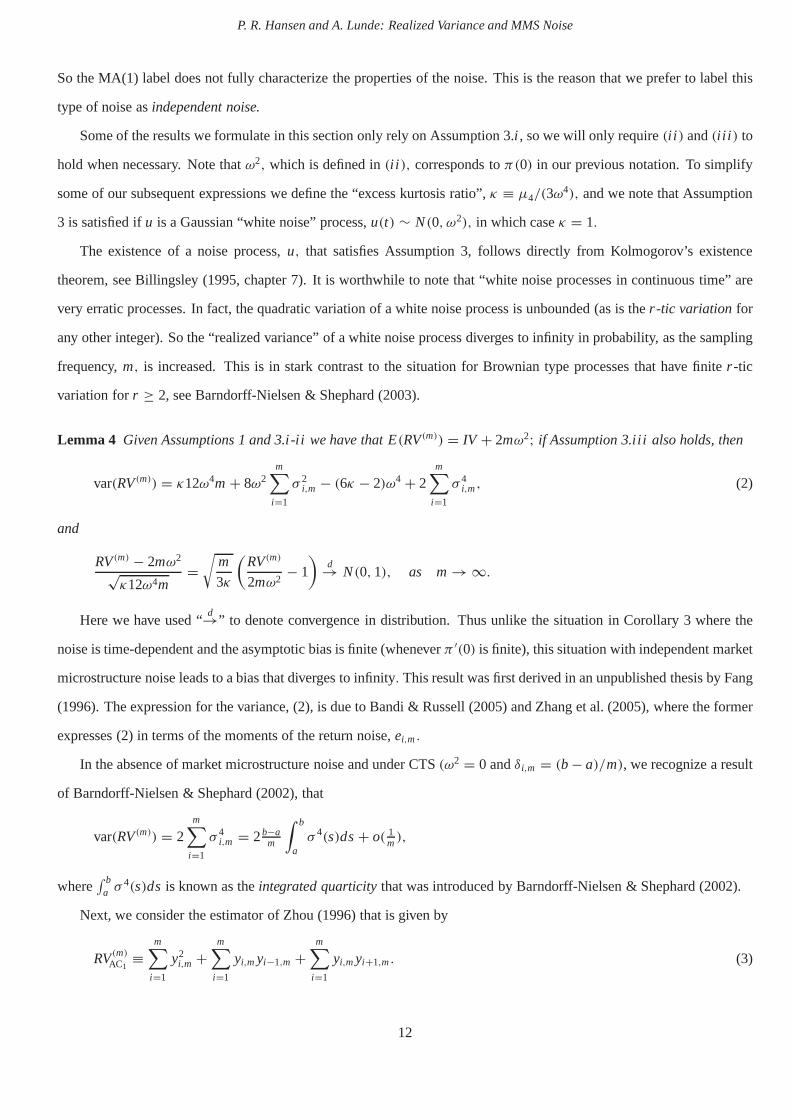
So the MA(1) label does not fully characterize the properties of the noise. This is the reason that we prefer to label this
type of noise asindependent noise.
Some of the results we formulate in this section only rely on Assumption 3.i , so we will only require(i i ) and(i i i ) to
hold when necessary. Note thatω2, which is defined in(i i ), corresponds toπ(0) in our previous notation. To simplify
some of our subsequent expressions we define the “excess kurtosis ratio”,κ ≡ µ4/(3ω4), and we note that Assumption
3 is satisfied ifu is a Gaussian “white noise” process,u(t) ∼ N(0, ω2), in which caseκ = 1.
The existence of a noise process,u, that satisfies Assumption 3, follows directly from Kolmogorov’s existence
theorem, see Billingsley (1995, chapter 7). It is worthwhile to note that “white noise processes in continuous time” are
very erratic processes. In fact, the quadratic variation ofa white noise process is unbounded (as is ther-tic variation for
any other integer). So the “realized variance” of a white noise process diverges to infinity in probability, as the sampling
frequency,m, is increased. This is in stark contrast to the situation for Brownian type processes that have finiter -tic
variation forr ≥ 2, see Barndorff-Nielsen & Shephard (2003).
Lemma 4 Given Assumptions 1 and 3.i-i i we have that E(RV(m)) = IV + 2mω2; if Assumption 3.i i i also holds, then
var(RV(m)) = κ12ω4m + 8ω2m∑
i=1
σ 2i,m − (6κ − 2)ω4 + 2
m∑
i=1
σ 4i,m, (2)
and
RV(m) − 2mω2
√κ12ω4m
=√
m
3κ
(RV(m)
2mω2− 1
)d→ N(0,1), as m→ ∞.
Here we have used “d→” to denote convergence in distribution. Thus unlike the situation in Corollary 3 where the
noise is time-dependent and the asymptotic bias is finite (wheneverπ ′(0) is finite), this situation with independent market
microstructure noise leads to a bias that diverges to infinity. This result was first derived in an unpublished thesis by Fang
(1996). The expression for the variance, (2), is due to Bandi& Russell (2005) and Zhang et al. (2005), where the former
expresses (2) in terms of the moments of the return noise,ei,m.
In the absence of market microstructure noise and under CTS(ω2 = 0 andδi,m = (b − a)/m), we recognize a result
of Barndorff-Nielsen & Shephard (2002), that
var(RV(m)) = 2m∑
i=1
σ 4i,m = 2b−a
m
∫ b
aσ 4(s)ds+ o( 1
m),
where∫ b
a σ4(s)ds is known as theintegrated quarticitythat was introduced by Barndorff-Nielsen & Shephard (2002).
Next, we consider the estimator of Zhou (1996) that is given by
RV(m)AC1≡
m∑
i=1
y2i,m +
m∑
i=1
yi,myi−1,m +m∑
i=1
yi,myi+1,m. (3)
12
P. R. Hansen and A. Lunde: Realized Variance and MMS Noise
This estimator incorporates the empirical first-order autocovariance, which amounts to a bias correction that ‘works’in
much the same way that robust covariance estimators, such asthat of Newey & West (1987), achieve their consistency.
Note that (3) involvesy0,m and ym+1,m that are intraday returns outside the interval[a,b]. If these two intraday returns
are unavailable, one could simply use the estimator∑m−1
i=2 y2i,m +
∑mi=2 yi,myi−1,m +
∑m−1i=1 yi,myi+1,m that estimates
∫ b−δm,m
a+δ1,mσ 2(s)ds = IV + O( 1
m). Here we follow Zhou (1996) and use the formulation in (3) because it simplifies the
analysis and several expressions. Our empirical implementation is based on a version that does not rely on intraday
returns that are outside the[a,b] interval. The exact implementation is described in the empirical section of this paper.
Next, we formulate results forRV(m)AC1that are similar to those forRV(m) in Lemma 4.
Lemma 5 Given Assumptions 1 and 3.i we have that E(RV(m)AC1) = IV; if Assumption 3.i i also holds then
var(RV(m)AC1) = 8ω4m + 8ω2
m∑
i=1
σ 2i,m − 6ω4 + 6
m∑
i=1
σ 4i,m + O(m−2),
under CTS and BTS, and
RV(m)AC1− IV
√8ω4m
d→ N(0,1), as m→ ∞.
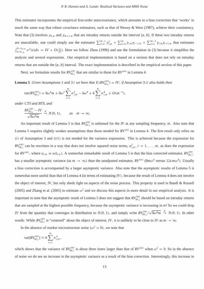
An important result of Lemma 5 is thatRV(m)AC1is unbiased for theIV at any sampling frequency,m. Also note that
Lemma 5 requires slightly weaker assumptions than those needed forRV(m) in Lemma 4. The first result only relies on
(i ) of Assumption 3 and(i i i ) is not needed for the variance expression. This is achieved because the expression for
RV(m)AC1can be rewritten in a way that does not involve squared noise terms,u2
i,m, i = 1, . . . ,m, as does the expression
for RV(m), whereui,m ≡ u(ti,m). A somewhat remarkable result of Lemma 5 is that the bias corrected estimator,RV(m)AC1,
has a smaller asymptotic variance (asm → ∞) than the unadjusted estimator,RV(m) (8mω4 versus 12κmω4). Usually
a bias correction is accompanied by a larger asymptotic variance. Also note that the asymptotic results of Lemma 5 is
somewhat more useful than that of Lemma 4 (in terms of estimating IV), because the result of Lemma 4 does not involve
the object of interest,IV, but only sheds light on aspects of the noise process. This property is used in Bandi & Russell
(2005) and Zhang et al. (2005) to estimateω2 and we discuss this aspects in more detail in our empirical analysis. It is
important to note that the asymptotic result of Lemma 5 does not suggest thatRV(m)AC1should be based on intraday returns
that are sampled at the highest possible frequency, becausethe asymptotic variance is increasing inm! So we could drop
IV from the quantity that converges in distribution toN(0,1), and simply writeRV(m)AC1/√
8ω4md→ N(0,1). In other
words: WhileRV(m)AC1is “centered” about the object of interest,IV, it is unlikely to be close toIV asm → ∞.
In the absence of market microstructure noise(ω2 = 0), we note that
var[RV(m)AC1] ≈ 6
m∑
i=1
σ 4i,m,
which shows that the variance ofRV(m)AC1is about three times larger than that ofRV(m) whenω2 = 0. So in the absence
of noise we do see an increase in the asymptotic variance as a result of the bias correction. Interestingly, this increasein
13
P. R. Hansen and A. Lunde: Realized Variance and MMS Noise
the variance is identical to that of the maximum likelihood estimator in a Gaussian specification whereσ 2(s) is constant
(andω2 = 0), see Aıt-Sahalia et al. (2005a).
It is easy to show thatτ ∗i = c/m, i = 1, . . . ,m solves the constrained minimization problem,
minτ1,...,τm
m∑
i=1
τ 2i subject to
m∑
i=1
τ i = c.
Thus, if we setτ i = σ 2i,m andc = IV, we see that
∑mi=1 σ
4i,m (for a fixedm) is minimized under BTS and this highlights
one of the advantages of BTS over CTS. This result was shown tohold in a related (pure jump) framework by Oomen
(2004a). In the present context we have under BTS that∑m
i=1 σ4i,m = IV2/m, and specifically it holds that
IV2/m ≤∫ b
aσ 4(s)dsb−a
m .
The variance expression under CTS (δi,m = (b − a)/m) is approximately given by
var[RV(m)AC1] ≈ 8ω4m + 8ω2
∫ b
aσ 2(s)− 6ω4 + 6b−a
m
∫ b
aσ 4(s)ds.
Next, we compareRV(m)AC1to RV(m) in terms of their mean square error (MSE) and their respective optimal sampling
frequencies for a special case that reveals key features of the two estimators.
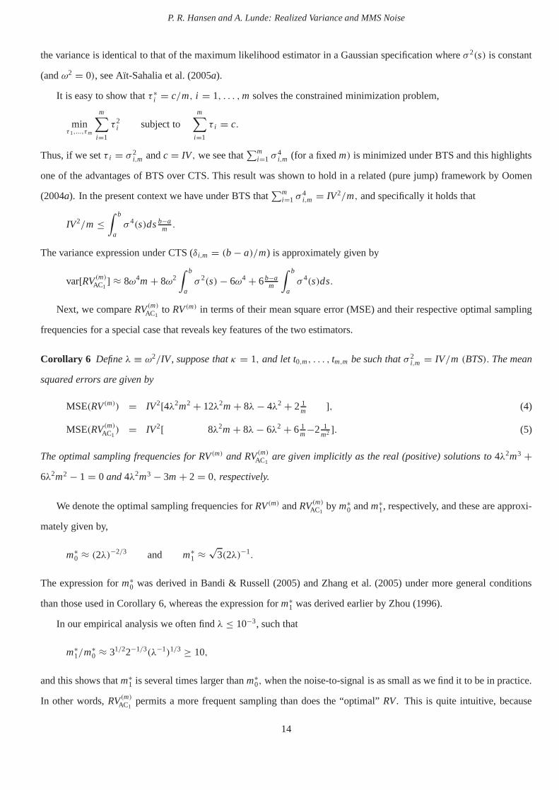
Corollary 6 Defineλ ≡ ω2/IV, suppose thatκ = 1, and let t0,m, . . . , tm,m be such thatσ 2i,m = IV/m (BTS). The mean
squared errors are given by
MSE(RV(m)) = IV2[4λ2m2 + 12λ2m + 8λ− 4λ2 + 2 1m ], (4)
MSE(RV(m)AC1) = IV2[ 8λ2m + 8λ− 6λ2 + 6 1
m−2 1m2 ]. (5)
The optimal sampling frequencies for RV(m) and RV(m)AC1are given implicitly as the real (positive) solutions to4λ2m3 +
6λ2m2 − 1 = 0 and4λ2m3 − 3m + 2 = 0, respectively.
We denote the optimal sampling frequencies forRV(m) andRV(m)AC1by m∗
0 andm∗1, respectively, and these are approxi-
mately given by,
m∗0 ≈ (2λ)−2/3 and m∗
1 ≈√
3(2λ)−1.
The expression form∗0 was derived in Bandi & Russell (2005) and Zhang et al. (2005) under more general conditions
than those used in Corollary 6, whereas the expression form∗1 was derived earlier by Zhou (1996).
In our empirical analysis we often findλ ≤ 10−3, such that
m∗1/m∗
0 ≈ 31/22−1/3(λ−1)1/3 ≥ 10,
and this shows thatm∗1 is several times larger thanm∗
0, when the noise-to-signal is as small as we find it to be in practice.
In other words,RV(m)AC1permits a more frequent sampling than does the “optimal”RV. This is quite intuitive, because
14
P. R. Hansen and A. Lunde: Realized Variance and MMS Noise
RV(m)AC1can utilize more information in the data without being affected by a severe bias. Naturally, when TTS is used
the number of intraday returns,m, cannot exceed the total number of transactions/quotations, so in practice it might
not be possible to sample as frequently as prescribed bym∗1. Furthermore, these results rely on the independent noise
assumption, which may not hold at the highest sampling frequencies.
Corollary 6 captures the salient features of this problem, and characterizes the MSE properties ofRV(m) andRV(m)AC1
in terms of a single parameter,λ, (noise-to-signal). Thus, the simplifying assumptions of Corollary 6 yield an attractive
framework for comparingRV(m) andRV(m)AC1, and for analyzing their (lack of) robustness to market microstructure noise.
FIGURE 3 ABOUT HERE
2000 Transaction data
[Top: RMSEs forRV andRVAC1]
[Middle: Relative efficiencies ofRV(m) andRV(m)AC1]
[Bottom: percentage increase of the RMSE that is due to noise]
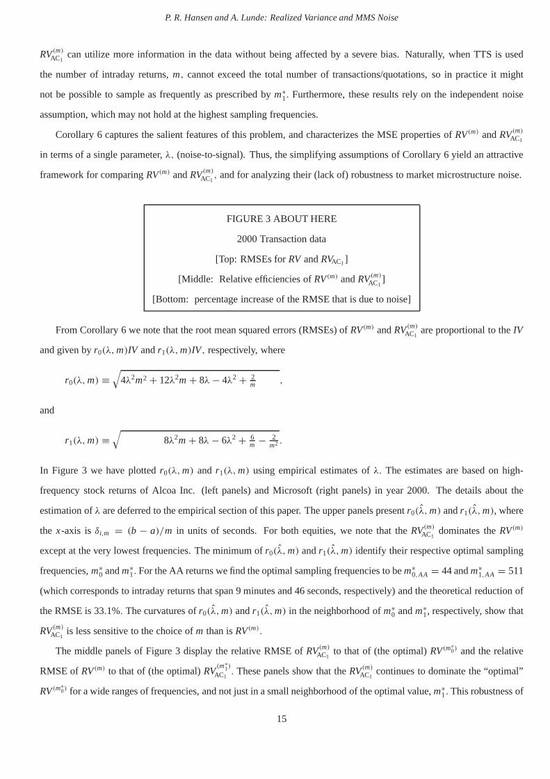
From Corollary 6 we note that the root mean squared errors (RMSEs) ofRV(m) andRV(m)AC1are proportional to theIV
and given byr0(λ,m)IV andr1(λ,m)IV, respectively, where
r0(λ,m) ≡√
4λ2m2 + 12λ2m + 8λ− 4λ2 + 2m ,
and
r1(λ,m) ≡√
8λ2m + 8λ− 6λ2 + 6m − 2
m2 .
In Figure 3 we have plottedr0(λ,m) and r1(λ,m) using empirical estimates ofλ. The estimates are based on high-
frequency stock returns of Alcoa Inc. (left panels) and Microsoft (right panels) in year 2000. The details about the
estimation ofλ are deferred to the empirical section of this paper. The upper panels presentr0(λ,m) andr1(λ,m), where
the x-axis is δi,m = (b − a)/m in units of seconds. For both equities, we note that theRV(m)AC1dominates theRV(m)
except at the very lowest frequencies. The minimum ofr0(λ,m) andr1(λ,m) identify their respective optimal sampling
frequencies,m∗0 andm∗
1. For the AA returns we find the optimal sampling frequencies tobem∗0,AA = 44 andm∗
1,AA = 511
(which corresponds to intraday returns that span 9 minutes and 46 seconds, respectively) and the theoretical reductionof
the RMSE is 33.1%. The curvatures ofr0(λ,m) andr1(λ,m) in the neighborhood ofm∗0 andm∗
1, respectively, show that
RV(m)AC1is less sensitive to the choice ofm than isRV(m).
The middle panels of Figure 3 display the relative RMSE ofRV(m)AC1to that of (the optimal)RV(m
∗0) and the relative
RMSE ofRV(m) to that of (the optimal)RV(m∗
1)
AC1. These panels show that theRV(m)AC1
continues to dominate the “optimal”
RV(m∗0) for a wide ranges of frequencies, and not just in a small neighborhood of the optimal value,m∗
1. This robustness of
15
P. R. Hansen and A. Lunde: Realized Variance and MMS Noise
RVAC1 is quite useful in practice whereλ and (hence)m∗1 are not known with certainty. The result shows that a reasonably
precise estimate ofλ (and hencem∗1) will lead to aRVAC1 that dominatesRV. This result is not surprising, because the
recent development in this literature has shown that it is possible to construct kernel-based estimators that are even more
accurate thanRVAC1, see Barndorff-Nielsen et al. (2004) and Zhang (2005).
A second very interesting aspect that can be analyzed from the results of Corollary 6, is the accuracy of theoretical
results that are derived under the assumption thatλ = 0 (no market microstructure noise). For example, the accuracy of a
confidence interval forIV, which is based on asymptotic results that ignores the presence of noise, will depend onλ and
m. The expressions of Corollary 6 provide a simple way to quantify the theoretical accuracy of such confidence intervals,
including those of Barndorff-Nielsen & Shephard (2002). Figure 3 provides valuable information about this question.
The upper panels of Figure 3 present the RMSEs ofRV(m) andRV(m)AC1, using both an estimateλ > 0 (the case with noise)
andλ = 0 (the case without noise). For small values ofm we see thatr0(λ,m) ≈ r0(0,m) andr1(λ,m) ≈ r1(0,m),
whereas the effects of market microstructure noise are pronounced at the higher sampling frequencies. The lower panels
of Figure 3 quantify the discrepancy between the two “types”of RMSEs as a function of the sampling frequency. These
plots present 100[r0(λ,m)− r0(0,m)]/r0(0,m) and 100[r1(λ,m)− r1(0,m)]/r1(0,m) as a function ofm. So the former
reveals the percentage increase of theRV’s RMSE, which is due to market microstructure noise, and thesecond line
similarly shows the increase of theRVAC1 ’s RMSE that is due to noise. The increase in the RMSE may be translated
into a widening of a confidence intervals forIV (aboutRV(m) or RV(m)AC1). The vertical lines in the right panels mark the
sampling frequency that corresponds to five-minute sampling under CTS, and these show that the “actual” confidence
interval (based onRV(m)) is 105.94% larger than the ‘no-noise’ confidence interval for AA, whereas the enlargement
is 22.37% for MSFT. At 20-minute sampling the discrepancy is less than a couple of percent, so in this case the size
distortion from being oblivious to market microstructure noise is quite small. The corresponding increases in the RMSE
of RV(m)AC1are 9.41% and 3.07%, respectively. So a ‘no-noise’ confidence interval aboutRV(m)AC1
is more reliable at moderate
sampling frequencies than that aboutRV(m). Here we have used an estimator ofλ that is based on data from the year
2000, before the tick size was reduced to one cent. In our empirical analysis we find the noise to be much smaller in
recent years, such that “no-noise approximations” are likely of be more accurate after the decimalization of the tick size.
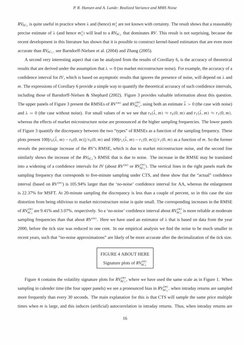
FIGURE 4 ABOUT HERE
Signature plots ofRV(m)AC1
Figure 4 contains the volatility signature plots forRV(m)AC1, where we have used the same scale as in Figure 1. When
sampling in calender time (the four upper panels) we see a pronounced bias inRV(m)AC1, when intraday returns are sampled
more frequently than every 30 seconds. The main explanationfor this is that CTS will sample the same price multiple
times whenm is large, and this induces (artificial) autocorrelation in intraday returns. Thus, when intraday returns are
16
P. R. Hansen and A. Lunde: Realized Variance and MMS Noise
based on CTS, it is necessary to incorporate higher-order autocovariances ofyi,m, whenm becomes large. The plots in
rows 3 and 4 are signature plots when intraday returns are sampled in tick-time. These also reveal a bias inRV(xtick)AC1
at
the highest frequencies, which shows that the noise is time dependent in tick time. For example, the MSFT 2000 plot
suggests that the time dependence lasts for 30 ticks – perhaps longer.
Fact II: The noise is autocorrelated.
We provide additional evidence of this fact in the followingsections, which is based on other empirical quantities.
4. The Case with Dependent Noise
In this section we consider the case where the noise is time-dependent and possibly correlated with the efficient returns,
y∗i,m. Following earlier versions of the present paper, issues that related to time-dependence and noise-price correlation
have been addressed in several other papers, including Aıt-Sahalia, Mykland & Zhang (2005b), Frijns & Lehnert (2004),
and Zhang (2005). The time-scale of the dependence in the noise plays a role in the asymptotic analysis. While the
“clock” at which the memory in the noise decays could follow any time scale, it seems reasonable that it is tied to
calendar-time, tick-time, or a combination of the two. First, we consider a situation where the time-dependence is
specific to calendar time, and then we consider the case with time-dependence in tick time.
4.1. Dependence in Calender Time
In order to bias correct theRV under the general time-dependent type of noise, we make the following assumption about
the time-dependence in the noise process.
Assumption 4 The noise process has finite dependence in the sense thatπ(s) = 0 for all s > θ0 for some finiteθ0 ≥ 0,
and E[u(t)|p∗(s)] = 0 for all |t − s| > θ0.
The assumption is trivially satisfied under the independentnoise assumption used in Section 3, while a more inter-
esting class of noise processes with finite dependence are those of the moving average type,u(t) =∫ t
t−θ0ψ(t −s)d B(s),
whereB(s) represents a standard Brownian motion andψ(s) is a bounded (non-random) function on[0, θ0]. The auto-
correlation function for a process of this kind is given byπ(s) =∫ θ0
s ψ(t)ψ(t − s)dt, for s ∈ [0, θ0].
Theorem 7 Suppose that Assumptions 1, 2, and 4 hold and let qm be such that qm/m> θ0. Then (under CTS)
E(RV(m)ACqm− IV) = 0,
where
RV(m)ACqm≡
m∑
i=1
y2i,m +
qm∑
h=1
m∑
i=1
(yi−h,myi,m + yi,myi+h,m).
17
P. R. Hansen and A. Lunde: Realized Variance and MMS Noise
A drawback ofRV(m)ACqmis that it may produce a negative estimate of volatility, because the covariances are not scaled
downwards in a way that would guarantee positivity. This is particularly relevant in the situation where intraday returns
have a “sharp negative autocorrelation”, see West (1997), which has been observed in high-frequency intraday returns
that are constructed from transaction prices. To rule out the possibility of a negative estimate one could use a different
kernel such as the Bartlett kernel. While a different kernelmay not be entirely unbiased, it may result is a smaller
mean squared error than that of theRVAC. Interestingly, Barndorff-Nielsen et al. (2004) have shown that the subsample
estimator of Zhang et al. (2005) is almost identical to the Bartlett-kernel estimator.
In the time-series literature the lag-length,qm, is typically chosen such thatqm/m → 0 asm → ∞, e.g.,qm =
⌈4(m/100)2/9⌉, where⌈x⌉ denotes the smallest integer that is greater than or equal tox. However, if the noise is
dependent in calendar time this would be inappropriate because this would lead toqm = 3 when a typical trading day
(390 minutes) is divided into 78 intraday returns (5-minutereturns), andqm = 6 if the day was divided into 780 intraday
returns (30-second returns). So the formerq would cover 15 minutes whereas the latter would cover 3 minutes (6× 30
seconds) and, in fact, the period shrinks to zero asm → ∞. Under Assumptions 2 and 4, the autocorrelation in intraday
returns is specific to a period in calendar time, which does not depend onm. So it is more appropriate to keep the width
of the “autocorrelation-window”,qmm , constant. This also makesRV(m)AC more comparable across different frequencies,m.
Thus we setqm = ⌈ w(b−a)/m⌉, wherew is the desired width of the lag window andb − a is the length of the sampling
period (both in units of time), such that(b − a)/m is the period covered by each intraday return. In this case wewill
write RV(m)ACw in place ofRV(m)ACqm. So if we sample in calendar time and setw = 15 min andb − a = 390 min, we would
includeqm = ⌈m/26⌉ autocovariance terms.
Whenqm is such thatqm/m> θ0 ≥ 0 it has the implication thatRV(m)ACqmcannot be consistent forIV. This property is
common for estimators of the long-run variance in the time-series literature, wheneverqm/m does not converge to zero
sufficiently fast, see e.g., Kiefer, Vogelsang & Bunzel (2000) and Jansson (2004). The lack of consistency in the present
context can be understood without consideration to market microstructure noise. In the absence of noise we have that
var(y2i,m) = 2σ 4
i,m and var(yi,myi+h,m) = σ 2i,mσ
2i+h,m ≈ σ 4
i,m, such that
var[RV(m)ACqm] ≈ 2
m∑
i=1
σ 4i,m +
qm∑
h=1
(2)2m∑
i=1
σ 4i,m
= 2(1 + 2qm)
m∑
i=1
σ 4i,m,
which approximately equals
2(1 + 2qm)b − a
m
∫ 1
0σ 4(s)ds,
under CTS. This shows that the variance does not vanish whenqm is such thatqm/m> θ0 > 0.
18
P. R. Hansen and A. Lunde: Realized Variance and MMS Noise
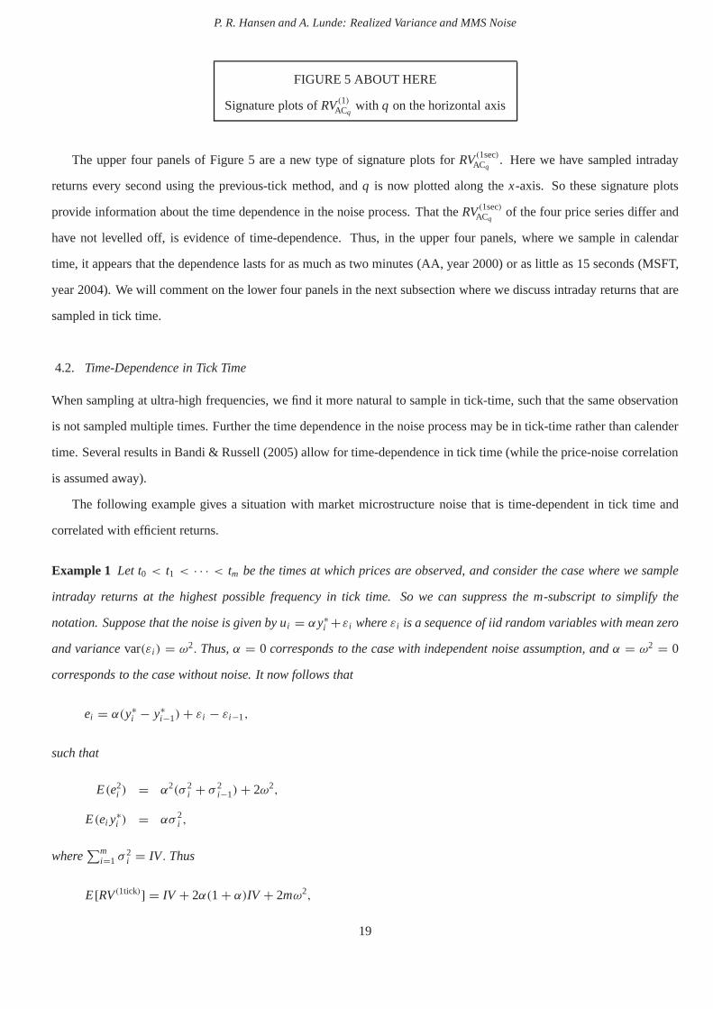
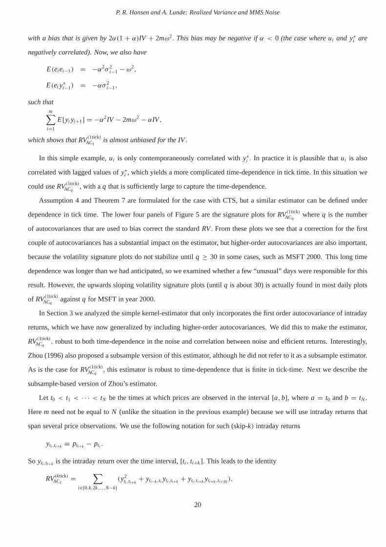
FIGURE 5 ABOUT HERE
Signature plots ofRV(1)ACqwith q on the horizontal axis
The upper four panels of Figure 5 are a new type of signature plots for RV(1sec)ACq
. Here we have sampled intraday
returns every second using the previous-tick method, andq is now plotted along thex-axis. So these signature plots
provide information about the time dependence in the noise process. That theRV(1sec)ACq
of the four price series differ and
have not levelled off, is evidence of time-dependence. Thus, in the upper four panels, where we sample in calendar
time, it appears that the dependence lasts for as much as two minutes (AA, year 2000) or as little as 15 seconds (MSFT,
year 2004). We will comment on the lower four panels in the next subsection where we discuss intraday returns that are
sampled in tick time.
4.2. Time-Dependence in Tick Time
When sampling at ultra-high frequencies, we find it more natural to sample in tick-time, such that the same observation
is not sampled multiple times. Further the time dependence in the noise process may be in tick-time rather than calender
time. Several results in Bandi & Russell (2005) allow for time-dependence in tick time (while the price-noise correlation
is assumed away).
The following example gives a situation with market microstructure noise that is time-dependent in tick time and
correlated with efficient returns.
Example 1 Let t0 < t1 < · · · < tm be the times at which prices are observed, and consider the case where we sample
intraday returns at the highest possible frequency in tick time. So we can suppress the m-subscript to simplify the
notation. Suppose that the noise is given by ui = αy∗i +εi whereεi is a sequence of iid random variables with mean zero
and variancevar(εi ) = ω2. Thus,α = 0 corresponds to the case with independent noise assumption,andα = ω2 = 0
corresponds to the case without noise. It now follows that
ei = α(y∗i − y∗
i−1)+ εi − εi−1,
such that
E(e2i ) = α2(σ 2
i + σ 2i−1)+ 2ω2,
E(ei y∗i ) = ασ 2
i ,
where∑m
i=1 σ2i = IV. Thus
E[RV(1tick)] = IV + 2α(1 + α)IV + 2mω2,
19
P. R. Hansen and A. Lunde: Realized Variance and MMS Noise
with a bias that is given by2α(1 + α)IV + 2mω2. This bias may be negative ifα < 0 (the case where ui and y∗i are
negatively correlated). Now, we also have
E(ei ei−1) = −α2σ 2i−1 − ω2,
E(ei y∗i−1) = −ασ 2
i−1,
such thatm∑
i=1
E[yi yi+1] = −α2IV − 2mω2 − αIV,
which shows that RV(1tick)AC1
is almost unbiased for the IV.
In this simple example,ui is only contemporaneously correlated withy∗i . In practice it is plausible thatui is also
correlated with lagged values ofy∗i , which yields a more complicated time-dependence in tick time. In this situation we
could useRV(1tick)ACq
, with aq that is sufficiently large to capture the time-dependence.
Assumption 4 and Theorem 7 are formulated for the case with CTS, but a similar estimator can be defined under
dependence in tick time. The lower four panels of Figure 5 arethe signature plots forRV(1tick)ACq
whereq is the number
of autocovariances that are used to bias correct the standard RV. From these plots we see that a correction for the first
couple of autocovariances has a substantial impact on the estimator, but higher-order autocovariances are also important,
because the volatility signature plots do not stabilize until q ≥ 30 in some cases, such as MSFT 2000. This long time
dependence was longer than we had anticipated, so we examined whether a few “unusual” days were responsible for this
result. However, the upwards sloping volatility signatureplots (untilq is about 30) is actually found in most daily plots
of RV(1tick)ACq
againstq for MSFT in year 2000.
In Section 3 we analyzed the simple kernel-estimator that only incorporates the first order autocovariance of intraday
returns, which we have now generalized by including higher-order autocovariances. We did this to make the estimator,
RV(1tick)ACq
, robust to both time-dependence in the noise and correlationbetween noise and efficient returns. Interestingly,
Zhou (1996) also proposed a subsample version of this estimator, although he did not refer to it as a subsample estimator.
As is the case forRV(1tick)ACq
, this estimator is robust to time-dependence that is finite in tick-time. Next we describe the
subsample-based version of Zhou’s estimator.
Let t0 < t1 < · · · < tN be the times at which prices are observed in the interval[a,b], wherea = t0 andb = tN .
Herem need not be equal toN (unlike the situation in the previous example) because we will use intraday returns that
span several price observations. We use the following notation for such (skip-k) intraday returns
yti ,ti+k ≡ pti+k − pti .
So yti ,ti+k is the intraday return over the time interval,[ti , ti+k]. This leads to the identity
RV(ktick)AC1
=∑
i∈{0,k,2k,...,N−k}(y2
ti ,ti+k+ yti−k,ti yti ,ti+k + yti ,ti+k yti+k,ti+2k),
20
P. R. Hansen and A. Lunde: Realized Variance and MMS Noise
(assuming thatN/k is an integer), which is a sum that involvesm = N/k terms. The subsample versionRV(m)AC1, which
was proposed by Zhou (1996) can be expressed as
1
k
N−1∑
i=0
(y2ti ,ti+k
+ yti−k,ti yti ,ti+k + yti ,ti+k yti+k,ti+2k). (6)
Thus, fork = 2 we have
1
2
N∑
i=1
(yi + yi+1)2 + (yi−1 + yi−2)(yi + yi+1)+ (yi + yi+1)(yi+2 + yi+3),
whereyi ≡ yti−1,ti , and by rearranging the terms, we see that this sum is approximately given by
1
2
N∑
i=1
2y2i + 4yi yi+1 + 4yi yi+2 + 2yi yi+3
= γ 0 + (γ−1 + γ 1)+ (γ−2 + γ 2)+ 1
2(γ−3 + γ 3),
whereγ j ≡∑N
i=1 yi yi+ j . For the general case,k ≥ 2, one can show that this subsample estimator is approximately
given by
RV(1tick)ACNWk
≡ γ 0 +k∑
j =1
(γ− j + γ j )+k∑
j =1
k− jk (γ− j −k + γ j +k).
So this estimator equals theRV(1tick)ACk
plus an additional term that is a Bartlett-type weighted sumof higher-order covari-
ances. Interestingly, Zhou (1996) showed that the subsample version of his estimator,(6), has a variance that is (at most)
of order O( kN ) + O(1
k ) + O( Nk2 ), (assuming constant volatility). This term is of orderO(N−1/3) if k is chosen to be
proportional toN2/3, as in Zhang et al. (2005). It appears that Zhou may have thought of k as fixed in his asymptotic
analysis, because he referred to this estimator as being inconsistent, see Zhou (1998, p.114). So the great virtues of
subsample-based estimators in this context were first recognized by Zhang et al. (2005).
5. Empirical Analysis
We analyze stock returns for the 30 equities of the Dow Jones Industrial Average (DJIA). The sample period spans five
years, from January 3, 2000 to December 31, 2004. We report results for each of the years individually, but some of
the more detailed results are only given for the years 2000 and 2004 to conserve space. The tick size was reduced from
a sixteenth of a dollar to one cent on January 29, 2001, and in order not to mix days with different tick sizes we drop
most of the days during January 2001 from our sample. The dataare transaction prices and quotations from NYSE and
NASDAQ and all data were extracted from the Trade and Quote (TAQ) database.
TABLE 1 ABOUT HERE
Data Description
21
P. R. Hansen and A. Lunde: Realized Variance and MMS Noise
The raw data were filtered for outliers and we discarded transactions outside the period from 9:30am to 4:00pm,
and days with less than five hours of trading were removed fromthe sample. This reduced the sample to the number
of days reported in the last column of Table 1. The filtering procedure removed obvious data error such as zero prices.
We also removed transaction prices that were more than one spread away from the bid and ask quotes. The exact
details of the filtering procedure is described in a technical appendix that is available from the authors website. The
average number of transactions/quotations per day are given for each of the years in our sample and these reveal a steady
increase in the number of transactions and quotations over the five year period. The numbers in parentheses are the
percentages of transaction prices that differ from the proceeding transaction price, and similarly for the quoted prices.
The same price is often observed in several consecutive transactions/quotations, because a large trade may be divided
into smaller transactions, and a “new” quote may simply reflect a revision of the “depth” while the bid and ask prices
remain unchanged. In our analysis we use all price observations. Censoring all the zero-intraday returns does not affect
theRV, but would have an impact on the autocorrelation of intradayreturns.
Our analysis of quotation data is based on bid and ask prices and the average of these (mid-quotes). TheRVs are
calculated for the hours that the market is open, approximately 390 minutes per day (6.5 hours for most days). We present
results for all 30 equities in our tables, whereas the figurespresent results for two equities: Alcoa Inc. (AA) and Microsoft
(MSFT), that represent equities of the DJIA with low and hightrading activities, respectively. The corresponding figures
for the other 28 DJIA equities are available upon request.
5.1. Empirical Implementation of Estimators
In practice, we will not rely on the intraday returns that areoutside the[a,b] interval. So in our empirical analysis we
have (forh > 0) substituted
γ h ≡ mm−h
m−h∑
i=1
yi,myi+h,m,
for the theoretical quantity,
γ h ≡m∑
i=1
yi,myi+h,m,
as the latter relies onym+1,m, . . . , ym+h,m. (For h < 0 we defineγ h ≡ γ |h|). In the expression forγ h we use an upward
scaling,m/(m − h), of the “autocovariances” to compensate for the “missing” autocovariance terms. So our empirical
implementation of the simplest kernel-estimator is given by RV(m)AC1=
∑mi=1 y2
i,m + 2 mm−1
∑m−1i=1 yi,myi+1,m.
22
P. R. Hansen and A. Lunde: Realized Variance and MMS Noise
5.2. Estimation of Market Microstructure Noise Parameters
Under the independent noise assumption used in Section 3, wehave from Lemma 4 that
ω2 ≡ RV(m)
2mp→ ω2, asm → ∞.
This estimator was proposed by Bandi & Russell (2005) and Zhang et al. (2005) for different purposes. Bandi & Russell
(2005) useω2t to determine the optimal sampling frequencym∗
0, whereas Zhang et al. (2005) employ the estimator to
select the number of subsamples and as a bias correction device of their “2nd best” one-scale subsample estimator.
Under the independent noise assumption we have from Lemma 4 that E(RV(m)) = IV + 2mω2, and whileω2 is
asymptotically justified, our empirical results reveal that ω2 is very small in practice. In fact, so small that 2mω2 is
small relative to theIV, with the exception of the most liquid assets, such as INTC andMSFT. Whenever theIV/2m is
non-negligbleω2 will over-estimateω2. So better estimators are given by
ω2 ≡ RV(m) − RV(13)
2(m − 13),
and
ω2 ≡ RV(m) − IV
2m,
whereRV(13) is based on intraday returns that span about 30 minutes each,and IV is some unbiased estimator ofIV.
From Lemmas 4 and 5 it follows thatω2, ω
2, andω2 are asymptotically equivalent in the sense that they have the same
probability limit asm → ∞. But ω2 and ω2 are unbiased forω2 for any finitem, and we will show thatω2 is quite
biased in many cases. Another problem is that the independent noise assumption need not hold at ultra-high frequencies,
in which case the asymptotic bias is not given by 2mω2. Clearly this is problematic for all three estimators.
TABLE 2 ABOUT HERE
OMEGAS
In Table 2 we present annual sample averages ofω2, ω
2, andω2, for the five years in our sample. Here we useRV(1tick)
AC1
as our choice forIV, which is unbiased under the independent noise assumption. The first estimator,ω2, assumes that
IV/2m is negligible, in which case all three estimators ought to besimilar. Becauseω2 andω2 generally agree whereas
ω2 is typically much larger, it is evident thatω2 overestimatesω2. A related observation was made in Engle & Sun
(2005).
Fact III: The noise is smaller than one might think.
23
P. R. Hansen and A. Lunde: Realized Variance and MMS Noise
That the noise in each of the intraday returns is relatively small (even when sampling occurs at the highest possible
frequency) is likely to affect the properties of the suggested implementation of the two-scale estimator by Zhang et al.
(2005). In fact the one-scale estimator that is proposed in Zhang et al. (2005) may be more accurate when the noise is
as small as Table 2 suggests. Similarly, when the optimal sampling frequency forRV is to be determined, as in Bandi &
Russell (2005), one should be careful not to overestimateω2, which would lead to a lower sampling frequency than the
optimal one. The important message is that one should incorporateRVAC1, or some other unbiased estimator ofIV, when
estimatingω2 from RV.
Another observation from Table 2 is that the noise has changed. For example our 2001 estimates ofω2 (usingω2)
are on average less than 20% of those of 2000, and even smallerin subsequent years. A large portion of this reduction is
due to the decimalization. We discuss the changed empiricalproperties of the noise in more detail in our discussion of
the results in Figures 6 and 7.
Now, if one were to believe the independent noise assumption, which is less of a stretch in 2000 than subsequent
years, one could construct the following estimate ofλ,
λ ≡ ω2/
IV ,
whereω2 ≡ n−1 ∑nt=1 ω
2t andIV ≡ n−1 ∑n
t=1 RV(1tick)AC1,t
. The latter is an estimate of the average dailyIV over the sample
t = 1, . . . ,n, becauseRVAC1 is unbiased forIV under the independent noise assumption. Similarly,ω2 is an estimate
of the average daily noise. If bothω2 and IV are constant across days, such thatλ is the same for all days, thenλ is
consistent forλ whenever a law of large numbers applies toω2t andRV(1tick)
AC1,t, t = 1, . . . ,n. In practice, bothω2 andIV
are likely to vary across days, soλ should only we viewed as a proxy for the noise-to-signal ratio.
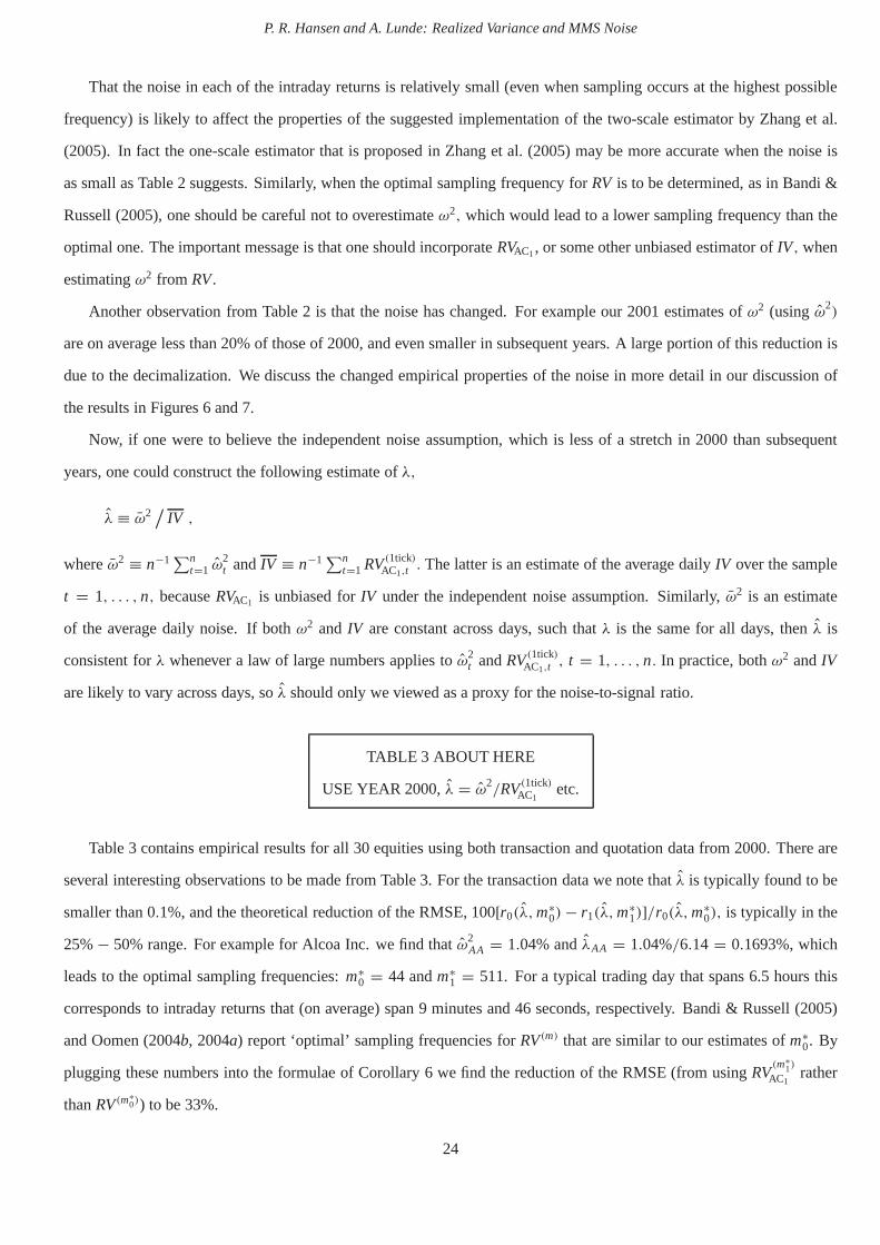
TABLE 3 ABOUT HERE
USE YEAR 2000,λ = ω2/RV(1tick)
AC1etc.
Table 3 contains empirical results for all 30 equities usingboth transaction and quotation data from 2000. There are
several interesting observations to be made from Table 3. For the transaction data we note thatλ is typically found to be
smaller than 0.1%, and the theoretical reduction of the RMSE, 100[r0(λ,m∗0)− r1(λ,m∗
1)]/r0(λ,m∗0), is typically in the
25%− 50% range. For example for Alcoa Inc. we find thatω2AA = 1.04% andλAA = 1.04%/6.14 = 0.1693%, which
leads to the optimal sampling frequencies:m∗0 = 44 andm∗
1 = 511. For a typical trading day that spans 6.5 hours this
corresponds to intraday returns that (on average) span 9 minutes and 46 seconds, respectively. Bandi & Russell (2005)
and Oomen (2004b, 2004a) report ‘optimal’ sampling frequencies forRV(m) that are similar to our estimates ofm∗0. By
plugging these numbers into the formulae of Corollary 6 we find the reduction of the RMSE (from usingRV(m∗
1)
AC1rather
thanRV(m∗0)) to be 33%.
24
P. R. Hansen and A. Lunde: Realized Variance and MMS Noise
The noise-to-signal ratio,λ, is likely to differ across days, in which case the optimal sampling frequencies,m∗0 and
m∗1, will also differ across days. Soλ should be viewed as a proxy forλ on a typical trading day, and our estimates above
should be viewed as approximations for “daily average values”, in the sense thatm0 = 90 andm1 = 1493 appear to be
sensible sampling frequencies to use with the MSFT transaction data. Fortunately, Figure 1 shows thatRV(m)AC1is relatively
insensitive to small deviations fromm∗1, such that a reasonable estimate forλ does produce a more accurate estimator
based onRVAC1 than one based onRV.
For the quotation data almost all our estimates ofω2 are negative, which occurs whenever the sample average of
RV(1 tick) is smaller than that ofRV(1tick)AC1
. This is obviously in conflict with the results of Lemmas 4 and 5that dictate
the population difference,E[RV(1tick) − RV(1tick)AC1
], to be positive. The expected difference is 2ω2 times a number that
is proportional to the average number of transactions/quotations per day. One explanation for observingω2< 0 is that
ω2 ≃ 0, such that the “wrong” sign simply occurs by chance. However, this is highly improbable because all but two of
the estimates ofω2 (and not just about half of them) are found to be negative for the quotation data. So these negative
estimates provide additional evidence against the independent noise assumption.
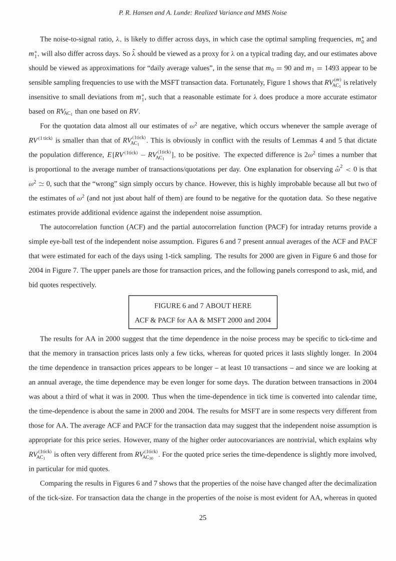
The autocorrelation function (ACF) and the partial autocorrelation function (PACF) for intraday returns provide a
simple eye-ball test of the independent noise assumption. Figures 6 and 7 present annual averages of the ACF and PACF
that were estimated for each of the days using 1-tick sampling. The results for 2000 are given in Figure 6 and those for
2004 in Figure 7. The upper panels are those for transaction prices, and the following panels correspond to ask, mid, and
bid quotes respectively.
FIGURE 6 and 7 ABOUT HERE
ACF & PACF for AA & MSFT 2000 and 2004
The results for AA in 2000 suggest that the time dependence inthe noise process may be specific to tick-time and
that the memory in transaction prices lasts only a few ticks,whereas for quoted prices it lasts slightly longer. In 2004
the time dependence in transaction prices appears to be longer – at least 10 transactions – and since we are looking at
an annual average, the time dependence may be even longer forsome days. The duration between transactions in 2004
was about a third of what it was in 2000. Thus when the time-dependence in tick time is converted into calendar time,
the time-dependence is about the same in 2000 and 2004. The results for MSFT are in some respects very different from
those for AA. The average ACF and PACF for the transaction data may suggest that the independent noise assumption is
appropriate for this price series. However, many of the higher order autocovariances are nontrivial, which explains why
RV(1tick)AC1
is often very different fromRV(1tick)AC30
. For the quoted price series the time-dependence is slightlymore involved,
in particular for mid quotes.
Comparing the results in Figures 6 and 7 shows that the properties of the noise have changed after the decimalization
of the tick-size. For transaction data the change in the properties of the noise is most evident for AA, whereas in quoted
25

P. R. Hansen and A. Lunde: Realized Variance and MMS Noise
prices the change is most pronounced for MSFT. For example, the first order autocovariances for bid and ask quotes have
opposite sign in 2000 and 2004. Thus, based on the results in Table 2 and Figures 6 and 7 we conclude that:
Fact IV: The properties of the noise have changed over time.
Because, the ACFs and PACFs we have plotted in Figures 6 and 7 are averages over daily estimates, there may be a
great deal of variation across days, although we did not find this to be the case in the daily ACFs and PACFs. For formal
hypothesis tests that address properties of market microstructure noise (day-by-day) see Awartani, Corradi & Distaso
(2004).
6. Price Decomposition by Cointegration Methods
Empirical studies on volatility estimation from contaminated high-frequency returns have typically used univariateprice
series, such as transaction prices, ask quotes, bid quotes,or mid quotes. All these series are proxies for the same efficient
price, and it is therefore natural to incorporate the information from all series, when estimating the volatility of thelatent
efficient price.
One way to combine the information from multiple series is tocompute aRV-type measure for each of these series
and take the average of these, as in Hansen & Lunde (2005c) who took the average of estimators that were based on
bid and ask quotes. Here we take a different approach and employ cointegration methods to extract the efficient price
(and noise) from a vector that consists of bid and ask quotes and transaction prices. This approach can be extended to
include additional price series. For example, limit order books can be used to define additional bid and ask price series
that depend on the volume that is offered at various prices, and prices from multiple exchanges could also be included in
the analysis.
The purpose of this analysis is threefold. First, the methodmakes it possible to decompose the different prices into
a common stochastic trend (efficient price) and transitory components (one noise process for each of the price series).
This makes it possible to compare the properties of these series to those we observe in our volatility signature plots.
Second, the decomposition reveals how the efficient price istied to innovations in the different price series. This shows
which of the price series are most informative about the efficient price. Third, we can study the dynamic impact on
quotes and transaction prices as a response to a change in theefficient price. This can be done with standard impulse
response analysis. For alternative ways to decompose the observed price series, see e.g. Engle & Sun (2005) who use
a ACD-GARCH specification where the noise process has a 2-component ARMA structure. See also Frijns & Lehnert
(2004).
We use the vector autoregressive framework that was used to analyze price discovery (from multiple markets) in
e.g. Harris, McInish, Shoesmith & Wood (1995), Hasbrouck (1995), and Harris, McInish & Wood (2002). Our analysis
26
P. R. Hansen and A. Lunde: Realized Variance and MMS Noise
differs from this literature because we apply cointegration techniques to quotes and transactions in conjunction, andnot
to transaction prices from different exchanges. Because itis possible to obtain the prevailing bid and ask prices at the
time that a transaction occurs, we avoid issues related to non-synchronous trading. Our impulse response analysis, which
we believe to be novel, shows how bid, ask, and transaction prices dynamically respond to a change in the efficient price.
We let ti , i = 0,1, . . . ,m denote the times where transactions occur during some trading day and we drop the
m-subscript to simplify the notation. We define the vector of “prices” by
pti =
transaction price at timeti
prevailing ask price at timeti
prevailing bid price at timeti
,
where we use log-prices as in the previous sections.
Suppose that the dynamics of the vector of prices,pti , can be approximated by the vector autoregressive error cor-
rection model,
1pti = αβ ′pti−1 +k−1∑
j =1
Ŵ j1pti− j + µ + εti , (7)
whereεti , i = 1, . . . ,m is a sequence of uncorrelated error terms. It is reasonable to assume that each of the three
observed price series share the same stochastic trend, suchthat any pair of prices cointegrate, as the spread is presumed
to be stationary. This implies thatα andβ are 3× 2 matrices with full column rank, and we may impose the two natural
cointegration vectors,
β = (β1,β2) =
1 0
−12 1
−12 −1
, (8)
The space spanned by the two columns ofβ define the set of cointegration relations. So any two linearly independent
vectors in this subspace can be used to defineβ.We choose these two vectors because they are simple to interpret: β ′1pti
is the difference between the transaction price and the mid-quote andβ ′2pti is the bid-ask spread.
Key in this analysis are the 3× 1 vectors,α⊥ andβ⊥, that are orthogonal toα andβ, respectively. (Thus,α′⊥α =
β ′⊥β = (0,0)). As is the case forα andβ these vectors are not fully identified, so we impose the normalizations
β⊥ = ι and α′⊥ι = 1,
whereι ≡ (1,1,1)′.
It follows from the Granger representation theorem that
pt = β⊥(α′⊥Ŵβ⊥)
−1α′⊥
t∑
s=1
εs + C(L)(εt + µ)+ A0,
27
P. R. Hansen and A. Lunde: Realized Variance and MMS Noise
whereŴ ≡ I−Ŵ1 −· · ·−Ŵk−1 andA0 is a term that depends on initial values ofpt . The Granger representation theorem
is due to Johansen (1988), and Hansen (2005) who obtained a recursive formula for the coefficients ofC(L) (and details
aboutA0), which will be used in our analysis.
6.1. Common Stochastic Trend
There are a number of ways to define thecommon stochastic trendfrom the Granger representation, see Johansen (1996).
The most natural definition in this framework is
p∗ti ≡ (α′
⊥Ŵβ⊥)−1
i∑
j =1
α′⊥εt j + initial value,
because this definition has the desired martingale property, as the corresponding intraday returns,
y∗ti
≡ α′⊥εti
α′⊥Ŵβ⊥
,
are uncorrelated. Thus, the Granger representation can be expressed as
pti =
p∗ti
p∗ti
p∗ti
+ C(L)εti + A0.
This definition of the common stochastic trend,p∗ti, corresponds to that of Hasbrouck (1995, 2002). Johansen (1996) also
discussed alternative definitions of the common stochastictrend, such asβ ′⊥pti andα′
⊥Ŵpti that are linear combinations of
the observed price vector. Such are known as Granger-Gonzalo stochastic trends in this literature, see Gonzalo & Granger
(1995). The connection betweenp∗ti
and a linear combination ofpti follows directly from the Granger representation, as
the latter involves a component that is proportional top∗ti and a second component that relates to the stationary part ofthe
Granger representation. This relation is discussed in Johansen (1996), see also Hansen & Johansen (1998, pp. 27-28),
and similar arguments later appeared in de Jong (2002) and Baillie, Booth, Tse & Zabotina (2002), see also Harris et al.
(2002) and Lehmann (2002).
It is the martingale property ofp∗ti that makes it the most natural definition of the efficient price, and theRV of p∗
ti is
given by
RVp∗ ≡m∑
i=1
(y∗ti )
2 =∑m
i=1(α′⊥εti )
2
(α′⊥Ŵβ⊥)
2.
Naturally, the parameters need to be estimated in practice,so we shall rely on
p∗ti = (α
′⊥Ŵβ⊥)
−1i∑
j =1
α′⊥εt j ,
whereεti are the residuals from (7). The estimation is described in Appendix C. Givenp∗ti, we can now define
RVp∗ ≡m∑
i=1
(y∗t j)2 =
∑mi=1(α
′⊥εti )
2
(α′⊥Ŵβ⊥)
2.
28
P. R. Hansen and A. Lunde: Realized Variance and MMS Noise
6.2. Empirical Results
We estimate the parameters in (7), for each of the days individually, where the number of lags,k, was chosen to be the
smallest number (≤ 10) that made Ljung-Box tests at lags 5, 10, 15, and 30 insignificant at the 5% significance level.
Some additional details about the estimation are given in Appendix C.
Assuming that the ultra high frequency price observations are well described by (7) is problematic for several reasons.
The duration between observations is an important aspect ofthe data that is ignored by model (7), and the discreteness
of the data have implications for the properties of the “errors” εti , i = 1, . . . ,m and the interdependence with the vector
of prices. The reader should be aware that, we have ignored all such issues. So the results we draw from this analysis
should be viewed as a rough approximation.
A key parameter in our analysis isα⊥ (3 × 1 vector) that shows how the efficient price is related to “innovations” in
the different price series. In our empirical analysis the elements ofα⊥ correspond to transaction prices, ask quotes, and
bid quotes respectively, so we use the following notation.
α′⊥ = (α⊥,tr., α⊥,ask, α⊥,bid).
TABLE 4 ABOUT HERE
Summary statistics: Lags,α⊥,t , α⊥,a, α⊥,b, RVp∗, RV(1tick)ACNW15
, RV(1tick)ACNW30
, RV(13)
.
RV(1tick)ACNWq
average of bid-ask-trans.
Sample Period: 2004
In Table 4 we report a summary of our empirical estimates, which are averages of the daily estimates,α⊥, andRVp∗ ,
for the sake of comparison, we also report the averageRV-quantities:RV(1tick)ACNW15
, RV(1tick)ACNW30
, andRV(13). To get a sense
of the dispersion of the daily estimates, we also report the 5% and 95% quantiles in brackets below each of the averages.
It is striking how similar the averageα⊥ is across equities that are listed on the NYSE – the average point estimates
are generally quite close toα⊥ = (12,
14,
14)
′. In contrast, the two NASDAQ stocks, INTC and MSFT, produce average
estimates that stands out by being closer toα⊥ = (14,
38,
38)
′. Thus the instantaneous correlation between innovations in
the transaction price and the efficient price is larger for NYSE stocks than for NASDAQ stocks – consequently, the quoted
prices are more closely related to the efficient price for NASDAQ stocks than is the case for NYSE stocks. We find this to
be a very interesting empirical observation that is likely to be tied to the differences by which the two exchanges operate.
Specifically that quotes on NASDAQ are competitive and binding, such that movements in these are more likely tied to
movements in the efficient price than is the case for the specialist quotes on the NYSE.
29
P. R. Hansen and A. Lunde: Realized Variance and MMS Noise
TABLE 5 ABOUT HERE
Summary statistics:RVp∗,∑m
i=1 e2ti and
∑mi=1 y∗
ti eti
Sample Period: 2004
The estimated model allows us to compute the daily estimates
m∑
i=1
e2ti and
m∑
i=1
y∗ti eti ,
whereeti is an element ofeti ≡ uti − uti−1 anduti = pti − p∗ti. (De-meaning the elements ofuti is not required as it does
not affecteti ). In Table 5 we report daily averages for the different price series.
FIGURE 8 ABOUT HERE
This figure illustrates a typical trading scenario for AA including p∗ti.
In Figure 8 we have plotted our estimate of the efficient price, p∗ti, for the same window of time that we plotted in
Figure 2. It is comforting to see that our estimate of the efficient price is in line with the quoted bid and ask prices. rarely
is p∗ti outside the bid-ask bounds, so there is no immediate evidence that a profit can be made from the discrepancies
betweenp∗ti
and the observed prices.
6.3. Impulse Response Function
Define the two matrices
5 = αβ ′ andC = β⊥(α′⊥Ŵβ⊥)
−1α′⊥.
As shown in Hansen (2005), the coefficients ofC(L) = C0+C1L+C2L2+· · · , are given recursively by the Yule-Walker
type equation
1Ci = 5Ci−1 + Ŵ11Ci−1 + · · · + Ŵk−11Ci−k+1, for i ≥ 1, (9)
where1Ci = Ci − Ci−1 andC0 = I − C, C−1 = C−2 = · · · = −C. An interesting question is how transaction prices
and quotes are affected by a change in the efficient price, this question can be addressed with reference to the Granger
representation.
While the Granger representation theorem is an algebraic result that does not rely on distributional assumptions,
interpretations drawn from it do rely on additional assumptions, see Hansen (2005). Under the restrictive Gaussian
assumptions, with homoskedastic innovations,� ≡ var(εti ), it follows that
dpti+h
dp∗ti
= dpti+h
dεti
× dεti
d(α′⊥εti )
× d(α′⊥εti )
dp∗ti
30
P. R. Hansen and A. Lunde: Realized Variance and MMS Noise
= (C + Ch)× �α⊥1
α′⊥�α⊥
× α′⊥Ŵβ⊥
= δ(C + Ch)�α⊥ = ι + δCh�α⊥,
where
δ ≡ α′⊥Ŵβ⊥
α′⊥�α⊥
.
Given the lack of results that hold under weaker (and more appropriate) assumptions, we will compute estimates of
ι + δCh�α⊥, h = 0,1, . . . , and interpret these as approximate impulse response functions. So these “projections”
should only be viewed as indicative of the dynamic effect on bid, ask, and transaction prices as a response to a change
in the efficient price. The long-run effect is unity for all prices – as it should be – sincedpti+h/dp∗ti
→ ι ash → ∞. This
follows from Ch → 0 ash → ∞, which holds under the standardI (1) assumptions, see e.g. Hansen (2005).
FIGURE 9 ABOUT HERE
This figure presentdpti+hdp∗
ti,h = 1, . . . ,100 for Bid, Ask, and Transaction prices, 2004 data.
[Left AA – right: MSFT]
Figure 9 displays the estimated impulse response functions(IRFs) for transaction prices, bid and ask quotes as a
response to a change in the efficient price. These results arebased on the daily estimates for 2004. The solid lines
correspond to the average IRFs, the dashed lines are the median IRF, and the shaded area is bounded by the 5% and 95%
quantiles across the days in 2004. While most of the price change occurs instantaneously, the estimated IRFs suggest that
it takes about ten transaction before the full effect is absorbed into transaction and quoted prices for AA, and only three
to five transactions for MSFT. Also note that the instantaneous effect on quotes is larger for MSFT than for AA (≈ 0.9
compared to≈ 0.8) and the total effect on quoted prices is absorbed quicker.This is likely explained by the differences
between specialist quotes on the NYSE and the competitive quotes on NASDAQ.
7. Summary and Concluding Remarks
We have analyzed the properties of market microstructure noise and its effect on empirical measures of volatility. Our
use of kernel-based estimators revealed several importantproperties about market microstructure noise, and we have
shown that kernel-based estimators are very useful in this context.
More importantly, our empirical analysis uncovered several characteristics of market microstructure noise, where the
most notable features are that the noise process is time-dependent and that the noise process is correlated with the latent
efficient returns. These results were established for both transaction data and quotation data and were found to hold for
intraday returns that are based on both calendar-time sampling and tick-time sampling.
31
P. R. Hansen and A. Lunde: Realized Variance and MMS Noise
We have also evaluated the accuracy of distributional results that are based on an assumption that there is no market
microstructure noise. We showed that a “no-noise” RMSE based on the results of Barndorff-Nielsen & Shephard (2002)
provide a reasonably accurate approximation when intradayreturns are sampled at low frequencies, such as 20-minute
sampling. At low sampling frequencies small sample issues can arise, such that coverage probabilities may be inaccurate,
see e.g. Goncalves & Meddahi (2005), but market microstructure noise is not to be blamed for such issues. When
intraday returns are sampled at higher frequencies the accuracy of “no-noise” approximations are likely to deteriorate.
The analogous ‘no-noise’ confidence interval aboutRV(m)AC1yields a more accurate approximation than that ofRV(m), but
both are very misleading when intraday returns are sampled at high frequencies.
Several results in the existing literature that analyze volatility estimation from high-frequency data that are contam-
inated with market microstructure noise have assumed that the noise process is independent of the efficient price and
uncorrelated in time. (Including our theoretical results in Section 3). Our empirical results suggest that the implications
of these assumptions may hold (at least approximately) whenintraday returns are sampled at relatively low frequencies.
So the conclusions of these papers may hold as long as intraday returns are not sampled more frequently than every 30
ticks, say. On the other hand, our empirical results have also shown that sampling at ultra high frequencies, such as every
few ticks, necessitates more general assumptions about thedependence structure of market microstructure noise. Such
results were established in Section 4 where we used a generalspecification for the noise process that can accommodate
both types of dependencies. Our cointegration analysis produced results that were consistent with both forms of depen-
dencies. Volatility signature plots revealed a negative noise-price correlation in quoted price series, and the cointegration
analysis showed that the negative correlation is found in all price series, including transaction prices.
While the main focus of our analysis has concerned the properties of market microstructure noise, our analysis also
provided some insight into the problem of volatility estimation in the presence of market microstructure noise. Under
the independent noise assumption, our comparison ofRV(m)AC1to the standard measure of realized variance revealed a
substantial improvement in the precision, as the theoretical reduction of the RMSE is about 25%-50%. These gains were
achieved with a simple bias correction that incorporates the first-order autocovariance, and additional improvementsare
possible with more sophisticated corrections of the realized variance. For example, the kernel-estimators of Barndorff-
Nielsen et al. (2004) and subsample estimators of Zhang et al. (2005) and Zhang (2005) are estimators that have better
asymptotic properties thanRV(m)AC1. Amongst the estimators we have analyzed in this paper,RV(1tick)
ACNW30appears to capture
the time-dependence that is found in the noise. However, there are potential gains from allowing for some bias in
exchange for a reduction of the variance. This may particularly be the case in recent years where we find the noise
(hence the bias) to be very small. Thus, correcting for a smaller number of autocovariances may be better in terms of the
RMSE, soRV(1tick)ACNW10
may be a better estimator thanRV(1tick)ACNW30
, although the former is more likely to be biased.
While the literature has made great progress on the problem of estimating the quadratic variation in the presence of
32
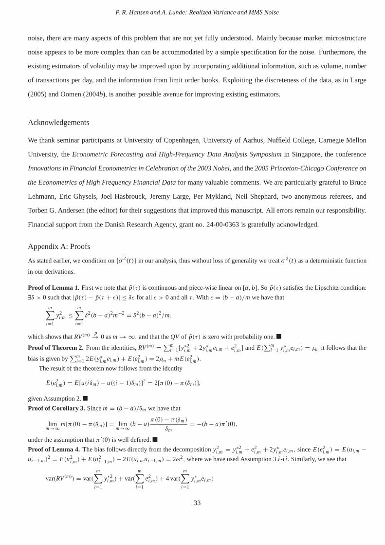
P. R. Hansen and A. Lunde: Realized Variance and MMS Noise
noise, there are many aspects of this problem that are not yetfully understood. Mainly because market microstructure
noise appears to be more complex than can be accommodated by asimple specification for the noise. Furthermore, the
existing estimators of volatility may be improved upon by incorporating additional information, such as volume, number
of transactions per day, and the information from limit order books. Exploiting the discreteness of the data, as in Large
(2005) and Oomen (2004b), is another possible avenue for improving existing estimators.
Acknowledgements
We thank seminar participants at University of Copenhagen,University of Aarhus, Nuffield College, Carnegie Mellon
University, theEconometric Forecasting and High-Frequency Data AnalysisSymposiumin Singapore, the conference
Innovations in Financial Econometrics in Celebration of the 2003 Nobel, and the2005 Princeton-Chicago Conference on
the Econometrics of High Frequency Financial Datafor many valuable comments. We are particularly grateful toBruce
Lehmann, Eric Ghysels, Joel Hasbrouck, Jeremy Large, Per Mykland, Neil Shephard, two anonymous referees, and
Torben G. Andersen (the editor) for their suggestions that improved this manuscript. All errors remain our responsibility.
Financial support from the Danish Research Agency, grant no. 24-00-0363 is gratefully acknowledged.
Appendix A: Proofs
As stated earlier, we condition on{σ 2(t)} in our analysis, thus without loss of generality we treatσ 2(t) as a deterministic function
in our derivations.
Proof of Lemma 1. First we note thatp(τ ) is continuous and piece-wise linear on[a,b]. So p(τ ) satisfies the Lipschitz condition:
∃δ > 0 such that| p(τ )− p(τ + ǫ)| ≤ δǫ for all ǫ > 0 and allτ . With ǫ = (b − a)/m we have that
m∑
i=1
y2i,m ≤
m∑
i=1
δ2(b − a)2m−2 = δ2(b − a)2/m,
which shows thatRV(m)p→ 0 asm → ∞, and that theQV of p(τ) is zero with probability one.
Proof of Theorem 2. From the identities,RV(m) =∑m
i=1[y∗2i,m + 2y∗
i,mei,m + e2i,m] andE(
∑mi=1 y∗
i,mei,m) = ρm it follows that the
bias is given by∑m
i=1 2E(y∗i,mei,m)+ E(e2
i,m) = 2ρm + mE(e2i,m).
The result of the theorem now follows from the identity
E(e2i,m) = E[u(i δm)− u((i − 1)δm)]2 = 2[π(0)− π(δm)],
given Assumption 2.
Proof of Corollary 3. Sincem = (b − a)/δm we have that
limm→∞
m[π(0)− π(δm)] = limm→∞
(b − a)π(0)− π(δm)
δm= −(b − a)π ′(0),
under the assumption thatπ ′(0) is well defined.
Proof of Lemma 4. The bias follows directly from the decompositiony2i,m = y∗2
i,m + e2i,m + 2y∗
i,mei,m, sinceE(e2i,m) = E(ui,m −
ui−1,m)2 = E(u2
i,m)+ E(u2i−1,m)− 2E(ui,mui−1,m) = 2ω2, where we have used Assumption 3.i -i i . Similarly, we see that
var(RV(m)) = var(m∑
i=1
y∗2i,m)+ var(
m∑
i=1
e2i,m)+ 4 var(
m∑
i=1
y∗i,mei,m)
33
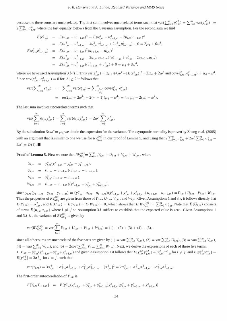
P. R. Hansen and A. Lunde: Realized Variance and MMS Noise
because the three sums are uncorrelated. The first sum involves uncorrelated terms such that var(∑m
i=1 y∗2i,m) =
∑mi=1 var(y∗2
i,m) =2
∑mi=1 σ
4i,m, where the last equality follows from the Gaussian assumption. For the second sum we find
E(e4i,m) = E(ui,m − ui−1,m)
4 = E(u2i,m + u2
i−1,m − 2ui,mui−1,m)2
= E(u4i,m + u4
i−1,m + 4u2i,mu2
i−1,m + 2u2i,mu2
i−1,m)+ 0 = 2µ4 + 6ω4,
E(e2i,me2
i+1,m) = E(ui,m − ui−1,m)2(ui+1,m − ui,m)
2
= E(u2i,m + u2
i−1,m − 2ui,mui−1,m)(u2i+1,m + u2
i,m − 2ui+1,mui,m)
= E(u2i,m + u2
i−1,m)(u2i+1,m + u2
i,m)+ 0 = µ4 + 3ω4,
where we have used Assumption 3.i -i i i . Thus var(e2i,m) = 2µ4+6ω4−[E(e2
i,m)]2 =2µ4 + 2ω4 and cov(e2i,m,e
2i+1,m) = µ4−ω4.
Since cov(e2i,m,e
2i+h,m) = 0 for |h| ≥ 2 it follows that
var(∑m
i=1e2
i,m) =∑m
i=1var(e2
i,m)+∑m
i, j =1i 6= j
cov(e2i,m,e
2j ,m)
= m(2µ4 + 2ω4)+ 2(m − 1)(µ4 − ω4) = 4mµ4 − 2(µ4 − ω4).
The last sum involves uncorrelated terms such that
var(m∑
i=1
ei,my∗i,m) =
m∑
i=1
var(ei,my∗i,m) = 2ω2
m∑
i=1
σ 2i,m.
By the substitution3κω4= µ4 we obtain the expression for the variance. The asymptotic normality is proven by Zhang et al. (2005)
with an argument that is similar to one we use forRV(m)AC1in our proof of Lemma 5, and using that 2
∑mi=1 σ
4i,m + 2ω2 ∑m
i=1 σ2i,m −
4ω4 = O(1).
Proof of Lemma 5. First we note thatRV(m)AC1=
∑mi=1Yi,m + Ui,m + Vi,m + Wi,m, where
Yi,m ≡ y∗i,m(y
∗i−1,m + y∗
i,m + y∗i+1,m),
Ui,m ≡ (ui,m − ui−1,m)(ui+1,m − ui−2,m),
Vi,m ≡ y∗i,m(ui+1,m − ui−2,m),
Wi,m ≡ (ui,m − ui−1,m)(y∗i−1,m + y∗
i,m + y∗i+1,m),
sinceyi,m(yi−1,m+yi,m+yi+1,m) = (y∗i,m+ui,m−ui−1,m)(y∗
i−1,m+y∗i,m+y∗
i+1,m+ui+1,m−ui−2,m) =Yi,m+Ui,m+Vi,m+Wi,m.
Thus the properties ofRV(m)AC1are given from those ofYi,m,Ui,m, Vi,m, andWi,m.Given Assumptions 1 and 3.i, it follows directly that
E(Yi,m) = σ 2i,m, andE(Ui,m) = E(Vi,m) = E(Wi,m) = 0, which shows thatE[RV(m)AC1
] =∑m
i=1 σ2i,m. Note thatE(Ui,m) consists
of termsE(ui,mu j ,m) wherei 6= j so Assumption 3.i suffices to establish that the expected value is zero. Given Assumptions 1
and 3.i -i i , the variance ofRV(m)AC1is given by
var[RV(m)AC1] = var[
m∑
i=1
Yi,m + Ui,m + Vi,m + Wi,m] = (1)+ (2)+ (3)+ (4)+ (5),
since all other sums are uncorrelated the five parts are givenby (1) = var(∑m
i=1 Yi,m), (2) = var(∑m
i=1 Ui,m), (3) = var(∑m
i=1 Vi,m),
(4) = var(∑m
i=1 Wi,m), and(5) = 2cov(∑m
i=1 Vi,m,∑m
i=1 Wi,m). Next, we derive the expressions of each of these five terms.
1. Yi,m = y∗i,m(y
∗i−1,m+y∗
i,m+y∗i+1,m) and given Assumption 1 it follows thatE[y∗2
i,my∗2j ,m] = σ 2
i,mσ2j ,m for i 6= j , andE[y∗2
i,my∗2j ,m] =
E[y∗4i,m] = 3σ 4
i,m for i = j , such that
var(Yi,m) = 3σ4i,m + σ 2
i,mσ2i−1,m + σ 2
i,mσ2i+1,m − [σ 2
i,m]2 = 2σ4i,m + σ 2
i,mσ2i−1,m + σ 2
i,mσ2i+1,m.
The first-order autocorrelation ofYi,m is
E[Yi,mYi+1,m] = E[y∗i,m(y
∗i−1,m + y∗
i,m + y∗i+1,m)y
∗i+1,m(y
∗i,m + y∗
i+1,m + y∗i+2,m)]
34
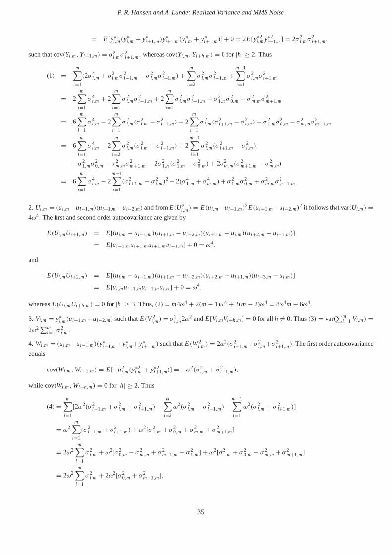
P. R. Hansen and A. Lunde: Realized Variance and MMS Noise
= E[y∗i,m(y
∗i,m + y∗
i+1,m)y∗i+1,m(y
∗i,m + y∗
i+1,m)] + 0 = 2E[y∗2i,my∗2
i+1,m] = 2σ 2i,mσ
2i+1,m,
such that cov(Yi,m,Yi+1,m) = σ 2i,mσ
2i+1,m, whereas cov(Yi,m,Yi+h,m) = 0 for |h| ≥ 2. Thus
(1) =m∑
i=1
(2σ 4i,m + σ 2
i,mσ2i−1,m + σ 2
i,mσ2i+1,m)+
m∑
i=2
σ 2i,mσ
2i−1,m +
m−1∑
i=1
σ 2i,mσ
2i+1,m
= 2m∑
i=1
σ 4i,m + 2
m∑
i=1
σ 2i,mσ
2i−1,m + 2
m∑
i=1
σ 2i,mσ
2i+1,m − σ 2
1,mσ20,m − σ 2
m,mσ2m+1,m
= 6m∑
i=1
σ 4i,m − 2
m∑
i=1
σ 2i,m(σ
2i,m − σ 2
i−1,m)+ 2m∑
i=1
σ 2i,m(σ
2i+1,m − σ 2
i,m)− σ 21,mσ
20,m − σ 2
m,mσ2m+1,m
= 6m∑
i=1
σ 4i,m − 2
m∑
i=2
σ 2i,m(σ
2i,m − σ 2
i−1,m)+ 2m−1∑
i=1
σ 2i,m(σ
2i+1,m − σ 2
i,m)
−σ 21,mσ
20,m − σ 2
m,mσ2m+1,m − 2σ 2
1,m(σ21,m − σ 2
0,m)+ 2σ2m,m(σ
2m+1,m − σ 2
m,m)
= 6m∑
i=1
σ 4i,m − 2
m−1∑
i=1
(σ 2i+1,m − σ 2
i,m)2 − 2(σ 4
1,m + σ 4m,m)+ σ 2
1,mσ20,m + σ 2
m,mσ2m+1,m
2. Ui,m = (ui,m−ui−1,m)(ui+1,m−ui−2,m) and fromE(U2i,m) = E(ui,m−ui−1,m)
2E(ui+1,m−ui−2,m)2 it follows that var(Ui,m) =
4ω4. The first and second order autocovariance are given by
E(Ui,mUi+1,m) = E[(ui,m − ui−1,m)(ui+1,m − ui−2,m)(ui+1,m − ui,m)(ui+2,m − ui−1,m)]= E[ui−1,mui+1,mui+1,mui−1,m] + 0 = ω4,
and
E(Ui,mUi+2,m) = E[(ui,m − ui−1,m)(ui+1,m − ui−2,m)(ui+2,m − ui+1,m)(ui+3,m − ui,m)]= E[ui,mui+1,mui+1,mui,m] + 0 = ω4,
whereasE(Ui,mUi+h,m) = 0 for |h| ≥ 3. Thus,(2) = m4ω4 + 2(m − 1)ω4 + 2(m − 2)ω4 = 8ω4m − 6ω4.
3. Vi,m = y∗i,m(ui+1,m−ui−2,m) such thatE(V2
i,m) = σ 2i,m2ω2 andE[Vi,mVi+h,m] = 0 for all h 6= 0. Thus(3) = var(
∑mi=1 Vi,m) =
2ω2 ∑mi=1 σ
2i,m.
4. Wi,m = (ui,m−ui−1,m)(y∗i−1,m+y∗
i,m+y∗i+1,m) such thatE(W2
i,m) = 2ω2(σ 2i−1,m+σ 2
i,m+σ 2i+1,m). The first order autocovariance
equals
cov(Wi,m,Wi+1,m) = E[−u2i,m(y
∗2i,m + y∗2
i+1,m)] = −ω2(σ 2i,m + σ 2
i+1,m),
while cov(Wi,m,Wi+h,m) = 0 for |h| ≥ 2. Thus
(4) =m∑
i=1
[2ω2(σ 2i−1,m + σ 2
i,m + σ 2i+1,m)−
m∑
i=2
ω2(σ 2i,m + σ 2
i−1,m)−m−1∑
i=1
ω2(σ 2i,m + σ 2
i+1,m)]
= ω2m∑
i=1
(σ 2i−1,m + σ 2
i+1,m)+ ω2[σ21,m + σ 2
0,m + σ 2m,m + σ 2
m+1,m]
= 2ω2m∑
i=1
σ 2i,m + ω2[σ 2
0,m − σ 2m,m + σ 2
m+1,m − σ 21,m] + ω2[σ2
1,m + σ 20,m + σ 2
m,m + σ 2m+1,m]
= 2ω2m∑
i=1
σ 2i,m + 2ω2[σ 2
0,m + σ 2m+1,m].
35
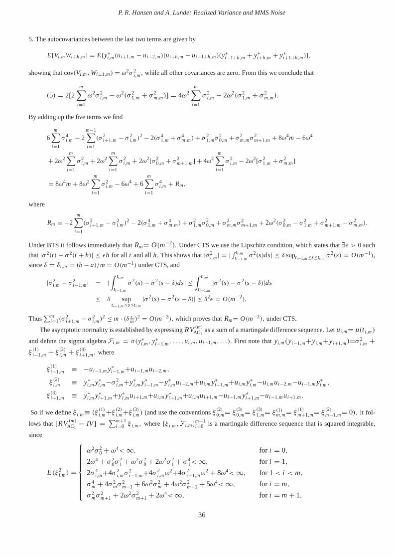
P. R. Hansen and A. Lunde: Realized Variance and MMS Noise
5. The autocovariances between the last two terms are given by
E[Vi,mWi+h,m] = E[y∗i,m(ui+1,m − ui−2,m)(ui+h,m − ui−1+h,m)(y
∗i−1+h,m + y∗
i+h,m + y∗i+1+h,m)],
showing that cov(Vi,m,Wi±1,m) = ω2σ 2i,m, while all other covariances are zero. From this we conclude that
(5) = 2[2m∑
i=1
ω2σ 2i,m − ω2(σ 2
1,m + σ 2m,m)] = 4ω2
m∑
i=1
σ 2i,m − 2ω2(σ 2
1,m + σ 2m,m).
By adding up the five terms we find
6m∑
i=1
σ 4i,m − 2
m−1∑
i=1
(σ 2i+1,m − σ 2
i,m)2 − 2(σ 4
1,m + σ 4m,m)+ σ 2
1,mσ20,m + σ 2
m,mσ2m+1,m + 8ω4m − 6ω4
+ 2ω2m∑
i=1
σ 2i,m + 2ω2
m∑
i=1
σ 2i,m + 2ω2[σ 2
0,m + σ 2m+1,m] + 4ω2
m∑
i=1
σ 2i,m − 2ω2[σ 2
1,m + σ 2m,m]
= 8ω4m + 8ω2m∑
i=1
σ 2i,m − 6ω4 + 6
m∑
i=1
σ 4i,m + Rm,
where
Rm ≡ −2m∑
i=1
(σ 2i+1,m − σ 2
i,m)2 − 2(σ 4
1,m + σ 4m,m)+ σ 2
1,mσ20,m + σ 2
m,mσ2m+1,m + 2ω2(σ 2
0,m − σ 21,m + σ 2
m+1,m − σ 2m,m).
Under BTS it follows immediately thatRm= O(m−2). Under CTS we use the Lipschitz condition, which states that∃ǫ > 0 such
that |σ 2(t) − σ 2(t + h)| ≤ ǫh for all t and allh. This shows that|σ2i,m| = |
∫ ti,mti−1,m
σ 2(s)ds| ≤ δ supti−1,m≤s≤ti,m σ2(s) = O(m−1),
sinceδ = δi,m = (b − a)/m = O(m−1) under CTS, and
|σ2i,m − σ 2
i−1,m| = |∫ ti,m
ti−1,m
σ 2(s)− σ 2(s − δ)ds| ≤∫ ti,m
ti−1,m
|σ2(s)− σ 2(s − δ)|ds
≤ δ supti−1,m≤s≤ti,m
|σ 2(s)− σ 2(s − δ)| ≤ δ2ǫ = O(m−2).
Thus∑m
i=1(σ2i+1,m − σ 2
i,m)2 ≤ m · (δ ǫm)2 = O(m−3), which proves thatRm= O(m−2), under CTS.
The asymptotic normality is established by expressingRV(m)AC1as a sum of a martingale difference sequence. Letui,m= u(t i,m)
and define the sigma algebraFi,m = σ(y∗i,m, y∗
i−1,m, . . . ,ui,m,ui−1,m, . . .). First note thatyi,m(yi−1,m+yi,m+yi+1,m)=σ 2i,m +
ξ(1)i−1,m + ξ
(2)i,m + ξ
(3)i+1,m, where
ξ(1)i−1,m ≡ −ui−1,my∗
i−1,m+ui−1,mui−2,m,
ξ(2)i,m ≡ y∗
i,my∗i,m−σ 2
i,m+y∗i,my∗
i−1,m−y∗i,mui−2,m+ui,my∗
i−1,m+ui,my∗i,m−ui,mui−2,m−ui−1,my∗
i,m,
ξ(3)i+1,m ≡ y∗
i,my∗i+1,m+y∗
i,mui+1,m+ui,my∗i+1,m+ui,mui+1,m−ui−1,my∗
i+1,m−ui−1,mui+1,m.
So if we defineξ i,m≡ (ξ(1)i,m+ξ (2)i,m+ξ (3)i,m) (and use the conventionsξ (2)0,m= ξ
(3)0,m= ξ
(3)1,m= ξ (1)m,m= ξ
(1)m+1,m= ξ
(2)m+1,m= 0), it fol-
lows that[RV(m)AC1− IV] =
∑m+1i=0 ξ i,m, where{ξ i,m,Fi,m}m+1
i=0 is a martingale difference sequence that is squared integrable,
since
E(ξ2i,m) =
ω2σ 20 + ω4< ∞, for i = 0,
2ω4 + σ 20σ
21 + ω2σ 2
0 + 2ω2σ 21 + σ 4
1< ∞, for i = 1,
2σ 4i,m+4σ 2
i,mσ2i−1,m+4σ 2
i,mω2+4σ 2
i−1,mω2 + 8ω4< ∞, for 1< i < m,
σ 4m + 4σ 2
mσ2m−1 + 6ω2σ 2
m + 4ω2σ 2m−1 + 5ω4< ∞, for i = m,
σ 2mσ
2m+1 + 2ω2σ 2
m+1 + 2ω4< ∞, for i = m + 1,
36
P. R. Hansen and A. Lunde: Realized Variance and MMS Noise
Sincem−1/2[RV(m)AC1− IV] = m−1/2 ∑m+1
i=0 ξ i,m, we can apply the central limit theorem for squared integrable martingales, see
Shiryaev (1995, p. 543, theorem 4), where the only remainingcondition to be verified, is the conditional Lindeberg condition:
m+1∑
i=0
E[m−1ξ2
i,m1{|m−1/2ξ i,m|>ε}|Fi−1,m
]p→ 0, asm → ∞.
SinceE[ξ2i,m1{|m−1/2ξ i,m|>ε}] is bounded byE[ξ2
i,m] < ∞ andsupi P(1{|ξ i,m|>ε√m}= 0) → 0, for all ε > 0, it follows that
E
∣∣∣∣∣m−1
m+1∑
i=0
ξ2i,m1{|m−1/2ξ i,m|>ε}−0
∣∣∣∣∣≤ m−1m+1∑
i=0
∣∣∣E[ξ2i,m1{|m−1/2ξ i,m|>ε}] − 0
∣∣∣ → 0, asm → ∞.
The Lindeberg condition now follows because convergence inL1 implies convergence in probability.
Proof of Corollary 6. The MSE’s are given from Lemmas 4 and 5, since BTS implies thatthe O(m−2) term in Lemma 5 (see the
proof of Lemma 5) is given by
Rm = 0 − 2(IV2/m2 + IV2/m2)+ IV2/m2 + IV2/m2 + 0 = −2IV2/m2.
Equating∂MSE(RV(m))/∂m_ 4λ2m + 6λ2 − m−2 with zero yields the first order condition of the corollary, and the second result
follows similarly from∂MSE(RV(m)AC1)/∂m_ 4λ2 − 3m−2 + 2m−3.
Proof of Theorem 7. Under CTS we can defineδm = (b − a)/m = ti,m − ti−1,m for all i = 1, . . . ,m. To simplify our notation, let
ui,m ≡ u(ti,m) and note that
E(ei,mei+h,m) = E[ui,m − ui−1,m][ui+h,m − ui+h−1,m]= 2π(hδm)− π((h − 1)δm)− π((h + 1)δm)
= [π(hδm)− π((h + 1)δm)] − [π((h − 1)δm)− π(hδm)],
such thatqm∑
h=1
E(ei,mei+h,m) = [π(qmδm)− π((qm + 1)δm)] − [π(0)− π(δm)],
where the first term equals zero given Assumption 4. Further,by Assumption 4 we have thaty∗i,m is uncorrelated with the noise
process when separated in time by at leastθ0. So that
0 = E[y∗i,m(ui+qm,m − ui−qm−1,m)] = E[y∗
i,m(ei+qm,m + · · · + ei−qm,m)],
and similarly,
0 = E[ei,m(y∗i+qm,m + · · · + y∗
i−qm,m)],
which implies that
ρm =m∑
i=1
E[y∗
i,mei,m]
= −m∑
i=1
qm∑
h=1
E[y∗i,mei+h,m + y∗
i,mei−h,m],
and
ρm =m∑
i=1
E[y∗
i,mei,m]
= −m∑
i=1
qm∑
h=1
E[ei,my∗i+h,m + ei,my∗
i−h,m],
Forh 6= 0 we have thatE(yi,myi+h,m) = (E[y∗
i,mei+h,m + ei,my∗i+h,m
]+ E(ei,mei+h,m), sinceE(y∗
i,my∗i+h,m) = 0 by Assumption
4. It now follows that
E[qm∑
h=1
m∑
i=1
yi,myi−h,m + yi,myi+h,m] = −2ρm − 2m[π(0)− π(δm)],
which proves thatRV(m)AC is unbiased.
37
P. R. Hansen and A. Lunde: Realized Variance and MMS Noise
Appendix B: Confidence Interval for Volatility Signature Plots
In our empirical analysis, we seek a measure that is informative about the precision of our bias correctedRVs. A minimum require-
ment is that the sample average ofRVAC is in a neighborhood of average integrated variance,
σ 2 ≡ n−1n∑
t=1
IVt ,
which may be estimated by
σ 2 = n−1n∑
t=1
IVt ,
where we useRV(1tick)ACNW30,t
as our choice forIVt , because it is likely to be conditionally unbiased forIVt . Next, we consider the
problem of constructing a confidence interval forσ 2. Andersen, Bollerslev, Diebold & Labys (2000a) and Andersen, Bollerslev,
Diebold & Labys (2003) have shown that the realized varianceis approximately log-normally distributed. Here we followthis idea
and assume that logIVt ∼ N(ξ , ω2), such that the unconditional expected value is given byE[IVt ] = σ 2 = exp(ξ + ω2/2) and
var(IVt ) = [exp(ω2)− 1] exp(ω2 + 2ξ).
Now, ξ ± σξc1−α/2 is a (1 − α)-confidence interval forξ, where ξ = n−1 ∑n
t=1 log IVt , σ 2ξ
≡ var(ξ ), and c1−α/2 is the
appropriate quantile from the standard normal distribution. Sinceξ = log(µ)− ω/2 it follows that,
P[l ≤ ξ ≤ u] = P[l + ω/2 ≤ log(σ 2) ≤ u + ω/2]= P[exp(l + ω/2) ≤ σ 2 ≤ exp(u + ω/2)],
such that the confidence interval forξ can be converted into one forσ 2. These calculations requireω2 to be known, while in practice
we must estimateω2. So we defineηt ≡ log IVt − ξ and use the Newey-West estimator,
ω2 ≡ 1
n − 1
n∑
t=1
η2t + 2
q∑
h=1
(1 − h
q + 1
)1
n − h
n−h∑
t=1
ηtηt+h, where q = int[4(n/100)2/9],
and subsequently setσ 2ξ
≡ ω2/n. An approximate confidence interval forσ 2 is now given by
CI(σ 2) ≡ exp(log(σ 2)± σ
ξc1−α/2),
which we recenter about log(σ 2) (rather thanξ + ω/2), because this ensures that the sample average ofIVt is inside the confidence
interval,σ 2 ∈ CI(σ 2).
Appendix C: Estimation of Cointegration VAR
To avoid a linear deterministic trend in the price series we impose the constraintµ = αρ whereρ = (ρ1, ρ2)′. (While a linear
deterministic trend may be quite sensible over a very long period, an estimate of such would be mostly spurious within a single day).
On the other hand, we do not want to exclude the constant entirely, as we do want to allow for a bid-ask spread to have a non-trivial
expected value, and this is fully accommodated by the restrictionµ = αρ.
While the model is simple to estimate by least squares when the constant in unrestricted or set to zero, the estimation under a
restricted constant is slightly more complicated.
1. Regress1pti on (p′ti−1
β, ι,1p′ti−1, . . . ,1p′
ti−k+1)′ by least squares and obtain(α, µ, Ŵ1, . . . , Ŵk−1).
2. Now set ρ = (α′α)−1α
′µ. (−ρ1 captures average difference between transaction prices and the mid-quotes, and−ρ2
captures ‘average’ spread between ask and bid quotes).
38
P. R. Hansen and A. Lunde: Realized Variance and MMS Noise
3. Regress1pti on (p′ti−1
β + ρ′,1p′
ti−1, . . . ,1p′
ti−k+1)′ by least squares and obtain(α, Ŵ1, . . . , Ŵk−1).
Define α⊥ ≡ 1ς[ι − α(α
′α)−1α
′ι],whereς ≡ ι′ι − ι′α(α′
α)−1α′ι. Then it follows thatα′
α⊥ = 1ς[α′
ι − α′α(α
′α)−1α
′ι] =
1ς[α′ι− α
′ι] = 0 andι′α⊥ = 1
ς[ι′ι − ι′α(α′
α)−1α′ι] = 1.
In the impulse response analysis we use the estimator� ≡ 1m
∑mi=1(εti − ε)(εti − ε)′.
References
Aıt-Sahalia, Y., Mykland, P. A. & Zhang, L. (2005a), ‘How often to sample a continuous-time process in the presence of
market microstructure noise’,Review of Financial Studies18, 351–416.
Aıt-Sahalia, Y., Mykland, P. A. & Zhang, L. (2005b), Ultra high frequency volatility estimation with dependent mi-
crostructure noise, Working Paper w11380, NBER.
Amihud, Y. & Mendelson, H. (1987), ‘Trading mechanisms and stock returns: An empirical investigation’,Journal of
Finance42(3), 533–553.
Andersen, T. G. & Bollerslev, T. (1997), ‘Intraday periodicity and volatility persistence in financial markets’,Journal of
Empirical Finance4, 115–158.
Andersen, T. G. & Bollerslev, T. (1998), ‘Answering the skeptics: Yes, standard volatility models do provide accurate
forecasts’,International Economic Review39(4), 885–905.
Andersen, T. G., Bollerslev, T. & Diebold, F. X. (2003), Somelike it smooth and some like it rough: Untangling
continuous and jump components in measuring, modeling and forecasting asset return volatility, Working paper,
Northwestern University, Duke University and University of Pennsylvania.
Andersen, T. G., Bollerslev, T., Diebold, F. X. & Ebens, H. (2001), ‘The distribution of realized stock return volatility’,
Journal of Financial Economics61(1), 43–76.
Andersen, T. G., Bollerslev, T., Diebold, F. X. & Labys, P. (2000a), ‘Exchange rate return standardized by realized
volatility are (nearly) Gaussian’,Multinational Finance Journal4(3&4), 159–179.
Andersen, T. G., Bollerslev, T., Diebold, F. X. & Labys, P. (2000b), ‘Great realizations’,Risk13(3), 105–108.
Andersen, T. G., Bollerslev, T., Diebold, F. X. & Labys, P. (2003), ‘Modeling and forecasting realized volatility’,Econo-
metrica71(2), 579–625.
Andersen, T. G., Bollerslev, T. & Meddahi, N. (2004), ‘Analytic evaluation of volatility forecasts’,International Eco-
nomic Review45, 1079–1110.
Andreou, E. & Ghysels, E. (2002), ‘Rolling-sample volatility estimators: Some new theoretical, simulation, and empiri-
cal results’,Journal of Business & Economic Statistics20(3), 363–376.
Andrews, D. W. K. (1991), ‘Heteroskedasticity and autocorrelation consistent covariance matrix estimation’,Economet-
rica 59, 817–858.
Awartani, B., Corradi, V. & Distaso, W. (2004), Testing and modelling market microstructure effects with an application
to the dow jones industrial average. Unpublished Manuscript, Queen Mary, University of London and University
of Exeter.
39
P. R. Hansen and A. Lunde: Realized Variance and MMS Noise
Bai, X., Russell, J. R. & Tiao, G. C. (2004), ‘Effects of non-normality and dependence on the precision of variance
estimates using high-frequency financial data’,Working paper, University of Chicago, GSB.
Baillie, R. T., Booth, G. G., Tse, Y. & Zabotina, T. (2002), ‘Price discovery and common factor models’,Journal of
Financial Markets5, 309–321.
Bandi, F. M. & Phillips, P. C. (2004), A simple approach to theparametric estimation of potentially nonstationary
diffusions. Unpublished Manuscript, University of Chicago and Yale University.
Bandi, F. M. & Russell, J. R. (2005), Microstructure noise, realized volatility, and optimal sampling, Working paper,
Graduate School of Business, The University of Chicago.
Barndorff-Nielsen, O. E., Hansen, P. R., Lunde, A. & Shephard, N. (2004), ‘Regular and modified kernel-based estima-
tors of integrated variance: The case with independent noise’.
http://www.stanford.edu/people/peter.hansen.
Barndorff-Nielsen, O. E., Nielsen, B., Shephard, N. & Ysusi, C. (1996), Measuring and forecasting financial variability
using realised variance with and without a model,in A. C. Harvey, S. J. Koopman & N. Shephard, eds, ‘State
Space and Unobserved Components Models: Theory and Applications’, Cambridge University Press, Cambridge,
pp. 205–235.
Barndorff-Nielsen, O. E. & Shephard, N. (2002), ‘Econometric analysis of realised volatility and its use in estimating
stochastic volatility models’,Journal of the Royal Statistical SocietyB 64, 253–280.
Barndorff-Nielsen, O. E. & Shephard, N. (2003), ‘Realized power variation and stochastic volatility’,Bernoulli 9, 243–
265.
Barndorff-Nielsen, O. E. & Shephard, N. (2004), ‘Power and bipower variation with stochastic volatility and jumps (with
discussion)’,Journal of Financial Econometrics2, 1–48.
Barndorff-Nielsen, O. E. & Shephard, N. (2005a), ‘Econometrics of testing for jumps in financial economicsusing
bipower variation’,Journal of Financial Econometrics. Forthcoming.
Barndorff-Nielsen, O. E. & Shephard, N. (2005b), ‘Impact of jumps on returns and realised variances: econometric
analysis of time-deformed lvy processes’,Journal of Econometrics. Forthcoming.
Billingsley, P. (1995),Probability and Measure, 3nd edn, John Wiley and Sons, New York.
Black, F. (1976), ‘Noise’,Journal of Finance41, 529–543.
Bollen, B. & Inder, B. (2002), ‘Estimating daily volatilityin financial markets utilizing intraday data’,Journal of Empir-
ical Finance9, 551–562.
Bollerslev, T., Kretschmer, U., Pigorsch, C. & Tauchen, G. (2005), The dynamics of bipower variation, realized volatility
and returns. Unpublished Manuscript, Department of Economics, Duke University.
Christensen, K. & Podolskij, M. (2005), Asymptotic Theory for Range-Based Estimation of Integrated Variance of a
Continuous Semi-Martingale, Working Paper, The Aarhus School of Business and Ruhr University of Bochum.
40
P. R. Hansen and A. Lunde: Realized Variance and MMS Noise
Corsi, F., Zumbach, G., Muller, U. & Dacorogna, M. (2001), ‘Consistent high-precision volatility from high-frequency
data’,Economic Notes30(2), 183–204.
Curci, G. & Corsi, F. (2004), Discrete sine transform approach for realized volatility measurement. Unpublished
Manuscript, Research Paper, University of Southern Switzerland.
Dacorogna, M. M., Gencay, R., Muller, U., Olsen, R. B. & Pictet, O. V. (2001),An Introduction to High-Frequency
Finance, Academic Press, London.
de Jong, F. (2002), ‘Measures of contributions to price discovery: a comparison’,Journal of Financial Markets5, 323–
327.
Easley, D. & O’Hara, M. (1987), ‘Price, trade size, and information in secturities markets’,Journal of Financial Eco-
nomics16, 69–90.
Easley, D. & O’Hara, M. (1992), ‘Time and the process of security price adjustment’,Journal of Finance47, 905–927.
Ebens, H. (1999), Realized stock volatility, Working paper420, Johns Hopkins University.
Engle, R. & Sun, Z. (2005), Forecasting volatility using tick by tick data. Unpublished Manuscript, New York University,
Stern School of Business.
Fang, Y. (1996), Volatility modeling and estimation of high-frequency data with Gaussian noise, Ph. d. thesis, MIT, Sloan
School of Management.
French, K. R., Schwert, G. W. & Stambaugh, R. F. (1987), ‘Expected stock returns and volatility’,Journal of Financial
Economics19(1), 3–29.
Frijns, B. & Lehnert, T. (2004), Realized variance in the presence of non-iid microstructure noise: A structural approach,
Wp04-008, Limburg Institute of Financial Economics.
Ghysels, E., Santa-Clara, P. & Valkanov, R. (2005), ‘Predicting volatility: getting the most out of return data sampledat
different frequencies’,Journal of Econometrics. Forthcoming.
Glosten, L. & Milgrom, P. (1985), ‘Bid, ask, and transactions prices in a specialist market with heterogeneously informed
traders’,Journal of Financial Economics13, 71–100.
Goncalves, S. & Meddahi, N. (2005), ‘Bootstrapping realized volatility’. manuscript, Departement de sciences
economiques, CIREQ and CIRANO, Universite de Montreal.
Gonzalo, J. & Granger, C. W. J. (1995), ‘Estimation of commonlong-memory components in cointegrated systems’,
Journal of Business & Economic Statistics13, 27–36.
Hansen, P. R. (2005), ‘Granger’s representation theorem: Aclosed-form expression forI (1) processes’,Econometrics
Journal8, 23–38.
Hansen, P. R. & Johansen, S. (1998),Workbook on Cointegration, Oxford University Press, Oxford.
41
P. R. Hansen and A. Lunde: Realized Variance and MMS Noise
Hansen, P. R. & Lunde, A. (2003), ‘An optimal and unbiased measure of realized variance based on intermittent high-
frequency data’. Mimeo prepared for the CIREQ-CIRANO Conference: Realized Volatility. Montreal, November
2003.
Hansen, P. R. & Lunde, A. (2005a), ‘Consistent ranking of volatility models’,Journal of Econometrics. Forthcoming.
Hansen, P. R. & Lunde, A. (2005b), ‘A forecast comparison of volatility models: Does anything beat a GARCH(1,1)?’,
Journal of Applied Econometrics. Forthcoming.
Hansen, P. R. & Lunde, A. (2005c), ‘A realized variance for the whole day based on intermittent high-frequency data’,
Journal of Financial Econometrics. Forthcoming.
Hansen, P. R., Lunde, A. & Nason, J. M. (2003), ‘Choosing the best volatility models: The model confidence set
approach’,Oxford Bulletin of Economics and Statistics65, 839–861.
Harris, F. H. D., McInish, T. H., Shoesmith, G. L. & Wood, R. A.(1995), ‘Cointegration, error correction, and price
discovery on informationally linked security markets’,Journal of Financial and Quantitative Analysis30(4), 563–
579.
Harris, F. H. D., McInish, T. H. & Wood, R. A. (2002), ‘Security price adjustment across exchanges: an investigation of
common factor components for dow stocks’,Journal of Financial Markets5(3), 277–308.
Harris, L. (1990), ‘Estimation of stock variance and serialcovariance from discrete observations’,Journal of Financial
and Quantitative Analysis25, 291–306.
Harris, L. (1991), ‘Stock price clustering and discreteness’, Review of Financial Studies4(3), 389–415.
Hasbrouck, J. (1995), ‘One security, many markets: determining the contributions to price discovery’,Journal of Finance
50, 1175–1198.
Hasbrouck, J. (2002), ‘Stalking the ”efficient price” in market microstructure specifications: an overview’,Journal of
Financial Markets5, 329–339.
Hasbrouck, J. (2004),Empirical Market Microstructure: Economic and Statistical Perspectives on the Dynamics of
Trade in Securities Markets. Lecture notes, Stern School of Business, New York University.
Huang, X. & Tauchen, G. (2004), The relative contribution ofjumps to total price variance. Unpublished Manuscript,
Department of Economics, Duke University.
Jacod, J. (1994), ‘Limit of random measures associated withthe increments of a Brownian semimartingale’. Unpublished
paper: Laboratorie de Probabilities, Universite P and M Curie, Paris.
Jacod, J. & Protter, P. (1998), ‘Asymptotic error distributions for the Euler method for stochastic differential equations’,
Annals of Probability26, 267–307.
Jansson, M. (2004), ‘The error in rejection probability of simple autocorrelation robust tests’,Econometrica72, 937–946.
Johansen, S. (1988), ‘Statistical analysis of cointegration vectors’,Journal of Economic Dynamics and Control12, 231–
254.
42
P. R. Hansen and A. Lunde: Realized Variance and MMS Noise
Johansen, S. (1996),Likelihood Based Inference in Cointegrated Vector Autoregressive Models, 2nd edn, Oxford Uni-
versity Press, Oxford.
Kiefer, N. M., Vogelsang, T. J. & Bunzel, H. (2000), ‘Simple robust testing of regression hypotheses’,Econometrica
68, 695–714.
Koopman, S. J., Jungbacker, B. & Hol, E. (2005), ‘Forecasting daily variability of the S&P 100 stock index using
historical, realised and implied volatility measurements’, Journal of Empirical Finance12, 445–475.
Large, J. (2005), Estimating quadratic variation when quoted prices jump by a constant increment. Nuffield College
Economics Group working paper W05.
Lehmann, B. (2002), ‘Some desiderata for the measurement ofprice discovery across markets’,Journal of Financial
Markets5, 259–276.
Maheu, J. M. & McCurdy, T. H. (2002), ‘Nonlinear features of realized FX volatility’,Review of Economics & Statistics
84, 668–681.
Meddahi, N. (2002), ‘A theoretical comparison between integrated and realized volatility’,Journal of Applied Econo-
metrics17, 479–508.
Merton, R. C. (1980), ‘On estimating the expected return on the market: An exploratory investigation’,Journal of
Financial Economics8, 323–361.
Muller, U. A. (1993), Statistics of variables observed over overlapping intervals, discussion paper, O&A Research Group.
Muller, U. A., Dacorogna, M. M., Olsen, R. B., Pictet, O. V.,Schwarz, M. & Morgenegg, C. (1990), ‘Statistical study of
foreign exchange rates, empirical evidence of a price change scaling law, and intraday analysis’,Journal of Banking
and Finance14, 1189–1208.
Newey, W. & West, K. (1987), ‘A simple positive semi-definite, heteroskedasticity and autocorrelation consistent covari-
ance matrix’,Econometrica55, 703–708.
O’Hara, M. (1995),Market Microstructure Theory, Blackwell.
Oomen, R. A. C. (2002), ‘Modelling realized variance when returns are serially correlated’. Manuscript, Warwick
Business School, The University of Warwick.
Oomen, R. A. C. (2004a), ‘Properties of bias corrected realized variance in calendar time and business time’. manuscript,
Warwick Business School, The University of Warwick.
Oomen, R. A. C. (2004b), ‘Properties of realized variance for a pure jump process:Calendar time sampling versus
business time sampling’. manuscript, Warwick Business School, The University of Warwick.
Owens, J. P. & Steigerwald, D. G. (2005), ‘Noise reduced realized volatility: A kalman filter approach’. Victoria
University of Wellington and University of California, Santa Barbara.
Patton, A. (2005), ‘Volatility forecast evaluation and comparison using imperfect volatility proxies’. Manuscript,London
School of Economics.
43
P. R. Hansen and A. Lunde: Realized Variance and MMS Noise
Protter, P. (2005),Stochastic Integration and Differential Equations, New York: Springer-Verlag.
Roll, R. (1984), ‘A simple implicit measure of the effectivebid-ask spread in an efficient market’,Journal of Finance
39, 1127–1139.
Shiryaev, A. N. (1995),Probability, 2nd edn, Springer-Verlag, New York.
Stein, M. L. (1987), ‘Minimum norm quadratic estimation of spatial variograms’,Journal of the American Statistical
Association82, 765–772.
Tauchen, G. & Zhou, H. (2004), Identifying realized jumps onfinancial markets. Unpublished Manuscript, Department
of Economics, Duke University.
Wasserfallen, W. & Zimmermann, H. (1985), ‘The behavior of intraday exchange rates’,Journal of Banking and Finance
9, 55–72.
West, K. D. (1997), ‘Another heteroskedasticity and autocorrelation consistent covariance matrix estimator’,Journal of
Econometrics76, 171–191.
Zhang, L. (2005), ‘Efficient estimation of stochastic volatility using noisy observations: A multi-scale approach’. Re-
search Paper, Carnegie Mellon University.
Zhang, L., Mykland, P. A. & Aıt-Sahalia, Y. (2005), ‘A tale of two time scales: Determining integrated volatility with
noisy high frequency data’,Journal of the American Statistical Association. Forthcoming.
Zhou, B. (1996), ‘High-frequency data and volatility in foreign-exchange rates’,Journal of Business & Economic Statis-
tics 14(1), 45–52.
Zhou, B. (1998), Parametric and nonparametric volatility measurement,in C. L. Dunis & B. Zhou, eds, ‘Nonlinear
Modelling of High Frequency Financial Time Series’, John Wiley Sons Ltd, chapter 6, pp. 109–123.
44
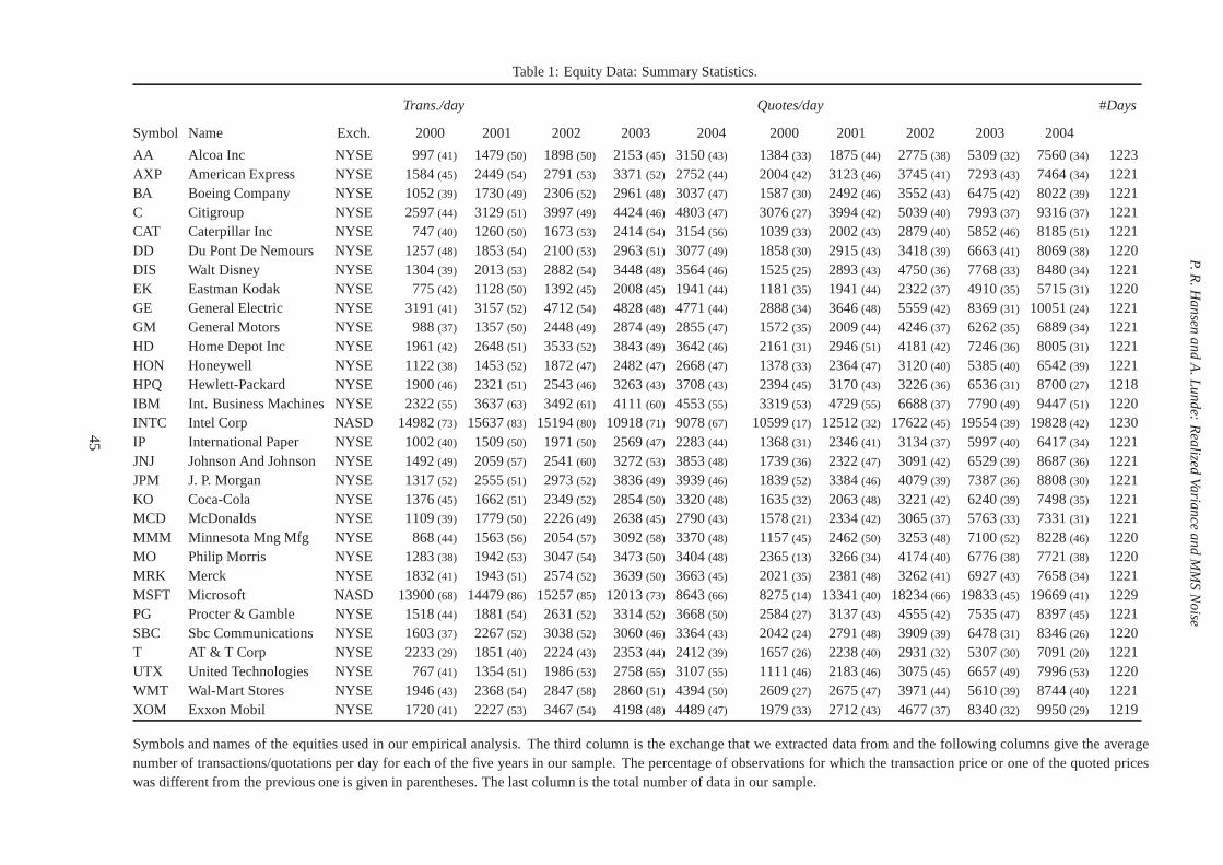
P.R.H
an
sen
an
dA
.Lu
nd
e:
Re
alize
dV
aria
nce
an
dM
MS
No
ise
Table 1: Equity Data: Summary Statistics.
Trans./day Quotes/day #Days
Symbol Name Exch. 2000 2001 2002 2003 2004 2000 2001 2002 20032004
AA Alcoa Inc NYSE 997(41) 1479(50) 1898(50) 2153(45) 3150(43) 1384(33) 1875(44) 2775(38) 5309(32) 7560(34) 1223AXP American Express NYSE 1584(45) 2449(54) 2791(53) 3371(52) 2752(44) 2004(42) 3123(46) 3745(41) 7293(43) 7464(34) 1221BA Boeing Company NYSE 1052(39) 1730(49) 2306(52) 2961(48) 3037(47) 1587(30) 2492(46) 3552(43) 6475(42) 8022(39) 1221C Citigroup NYSE 2597(44) 3129(51) 3997(49) 4424(46) 4803(47) 3076(27) 3994(42) 5039(40) 7993(37) 9316(37) 1221CAT Caterpillar Inc NYSE 747(40) 1260(50) 1673(53) 2414(54) 3154(56) 1039(33) 2002(43) 2879(40) 5852(46) 8185(51) 1221DD Du Pont De Nemours NYSE 1257(48) 1853(54) 2100(53) 2963(51) 3077(49) 1858(30) 2915(43) 3418(39) 6663(41) 8069(38) 1220DIS Walt Disney NYSE 1304(39) 2013(53) 2882(54) 3448(48) 3564(46) 1525(25) 2893(43) 4750(36) 7768(33) 8480(34) 1221EK Eastman Kodak NYSE 775(42) 1128(50) 1392(45) 2008(45) 1941(44) 1181(35) 1941(44) 2322(37) 4910(35) 5715(31) 1220GE General Electric NYSE 3191(41) 3157(52) 4712(54) 4828(48) 4771(44) 2888(34) 3646(48) 5559(42) 8369(31) 10051(24) 1221GM General Motors NYSE 988(37) 1357(50) 2448(49) 2874(49) 2855(47) 1572(35) 2009(44) 4246(37) 6262(35) 6889(34) 1221HD Home Depot Inc NYSE 1961(42) 2648(51) 3533(52) 3843(49) 3642(46) 2161(31) 2946(51) 4181(42) 7246(36) 8005(31) 1221HON Honeywell NYSE 1122(38) 1453(52) 1872(47) 2482(47) 2668(47) 1378(33) 2364(47) 3120(40) 5385(40) 6542(39) 1221HPQ Hewlett-Packard NYSE 1900(46) 2321(51) 2543(46) 3263(43) 3708(43) 2394(45) 3170(43) 3226(36) 6536(31) 8700(27) 1218IBM Int. Business Machines NYSE 2322(55) 3637(63) 3492(61) 4111(60) 4553(55) 3319(53) 4729(55) 6688(37) 7790(49) 9447(51) 1220INTC Intel Corp NASD 14982(73) 15637(83) 15194(80) 10918(71) 9078(67) 10599(17) 12512(32) 17622(45) 19554(39) 19828(42) 1230IP International Paper NYSE 1002(40) 1509(50) 1971(50) 2569(47) 2283(44) 1368(31) 2346(41) 3134(37) 5997(40) 6417(34) 1221JNJ Johnson And Johnson NYSE 1492(49) 2059(57) 2541(60) 3272(53) 3853(48) 1739(36) 2322(47) 3091(42) 6529(39) 8687(36) 1221JPM J. P. Morgan NYSE 1317(52) 2555(51) 2973(52) 3836(49) 3939(46) 1839(52) 3384(46) 4079(39) 7387(36) 8808(30) 1221KO Coca-Cola NYSE 1376(45) 1662(51) 2349(52) 2854(50) 3320(48) 1635(32) 2063(48) 3221(42) 6240(39) 7498(35) 1221MCD McDonalds NYSE 1109(39) 1779(50) 2226(49) 2638(45) 2790(43) 1578(21) 2334(42) 3065(37) 5763(33) 7331(31) 1221MMM Minnesota Mng Mfg NYSE 868(44) 1563(56) 2054(57) 3092(58) 3370(48) 1157(45) 2462(50) 3253(48) 7100(52) 8228(46) 1220MO Philip Morris NYSE 1283(38) 1942(53) 3047(54) 3473(50) 3404(48) 2365(13) 3266(34) 4174(40) 6776(38) 7721(38) 1220MRK Merck NYSE 1832(41) 1943(51) 2574(52) 3639(50) 3663(45) 2021(35) 2381(48) 3262(41) 6927(43) 7658(34) 1221MSFT Microsoft NASD 13900(68) 14479(86) 15257(85) 12013(73) 8643(66) 8275(14) 13341(40) 18234(66) 19833(45) 19669(41) 1229PG Procter & Gamble NYSE 1518(44) 1881(54) 2631(52) 3314(52) 3668(50) 2584(27) 3137(43) 4555(42) 7535(47) 8397(45) 1221SBC Sbc Communications NYSE 1603(37) 2267(52) 3038(52) 3060(46) 3364(43) 2042(24) 2791(48) 3909(39) 6478(31) 8346(26) 1220T AT & T Corp NYSE 2233(29) 1851(40) 2224(43) 2353(44) 2412(39) 1657(26) 2238(40) 2931(32) 5307(30) 7091(20) 1221UTX United Technologies NYSE 767(41) 1354(51) 1986(53) 2758(55) 3107(55) 1111(46) 2183(46) 3075(45) 6657(49) 7996(53) 1220WMT Wal-Mart Stores NYSE 1946(43) 2368(54) 2847(58) 2860(51) 4394(50) 2609(27) 2675(47) 3971(44) 5610(39) 8744(40) 1221XOM Exxon Mobil NYSE 1720(41) 2227(53) 3467(54) 4198(48) 4489(47) 1979(33) 2712(43) 4677(37) 8340(32) 9950(29) 1219
Symbols and names of the equities used in our empirical analysis. The third column is the exchange that we extracted data from and the following columns give the averagenumber of transactions/quotations per day for each of the five years in our sample. The percentage of observations for which the transaction price or one of the quoted priceswas different from the previous one is given in parentheses.The last column is the total number of data in our sample.
45
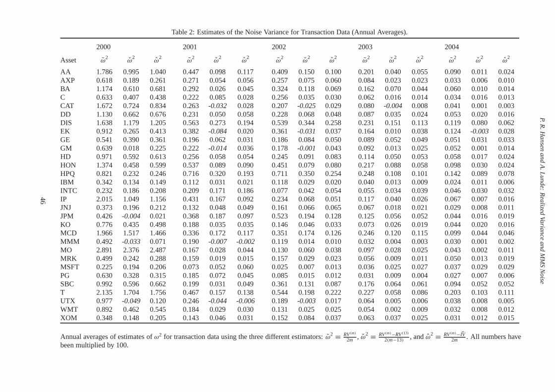
P.R.H
an
sen
an
dA
.Lu
nd
e:
Re
alize
dV
aria
nce
an
dM
MS
No
ise
Table 2: Estimates of the Noise Variance for Transaction Data (Annual Averages).
2000 2001 2002 2003 2004
Asset ω2
ω2
ω2
ω2
ω2
ω2
ω2
ω2
ω2
ω2
ω2
ω2
ω2
ω2
ω2
AA 1.786 0.995 1.040 0.447 0.098 0.117 0.409 0.150 0.100 0.201 0.040 0.055 0.090 0.011 0.024AXP 0.618 0.189 0.261 0.271 0.054 0.056 0.257 0.075 0.060 0.084 0.023 0.023 0.033 0.006 0.010BA 1.174 0.610 0.681 0.292 0.026 0.045 0.324 0.118 0.069 0.162 0.070 0.044 0.060 0.010 0.014C 0.633 0.407 0.438 0.222 0.085 0.028 0.256 0.035 0.030 0.0620.016 0.014 0.034 0.016 0.013CAT 1.672 0.724 0.834 0.263 -0.032 0.028 0.207 -0.025 0.029 0.080 -0.004 0.008 0.041 0.001 0.003DD 1.130 0.662 0.676 0.231 0.050 0.058 0.228 0.068 0.048 0.087 0.035 0.024 0.053 0.020 0.016DIS 1.638 1.179 1.205 0.563 0.273 0.194 0.539 0.344 0.258 0.231 0.151 0.113 0.119 0.080 0.062EK 0.912 0.265 0.413 0.382 -0.084 0.020 0.361 -0.031 0.037 0.164 0.010 0.038 0.124-0.003 0.028GE 0.541 0.390 0.361 0.196 0.062 0.031 0.186 0.084 0.050 0.089 0.052 0.049 0.051 0.031 0.033GM 0.639 0.018 0.225 0.222 -0.014 0.036 0.178 -0.001 0.043 0.092 0.013 0.025 0.052 0.001 0.014HD 0.971 0.592 0.613 0.256 0.058 0.054 0.245 0.091 0.083 0.114 0.050 0.053 0.058 0.017 0.024HON 1.374 0.458 0.599 0.537 0.089 0.090 0.451 0.079 0.080 0.217 0.088 0.058 0.098 0.030 0.024HPQ 0.821 0.232 0.246 0.716 0.320 0.193 0.711 0.350 0.254 0.248 0.108 0.101 0.142 0.089 0.078IBM 0.342 0.134 0.149 0.112 0.031 0.021 0.118 0.029 0.020 0.040 0.013 0.009 0.024 0.011 0.006INTC 0.232 0.186 0.208 0.209 0.171 0.186 0.077 0.042 0.054 0.055 0.034 0.039 0.046 0.030 0.032IP 2.015 1.049 1.156 0.431 0.167 0.092 0.234 0.068 0.051 0.117 0.040 0.026 0.067 0.007 0.016JNJ 0.373 0.196 0.212 0.132 0.048 0.049 0.161 0.066 0.065 0.067 0.018 0.021 0.029 0.008 0.011JPM 0.426 -0.004 0.021 0.368 0.187 0.097 0.523 0.194 0.128 0.125 0.056 0.052 0.044 0.016 0.019KO 0.776 0.435 0.498 0.188 0.035 0.035 0.146 0.046 0.033 0.073 0.026 0.019 0.044 0.020 0.016MCD 1.966 1.517 1.466 0.336 0.172 0.117 0.351 0.174 0.126 0.246 0.120 0.115 0.099 0.044 0.046MMM 0.492 -0.033 0.071 0.190 -0.007 -0.002 0.119 0.014 0.010 0.032 0.004 0.003 0.030 0.001 0.002MO 2.891 2.376 2.487 0.167 0.028 0.044 0.130 0.060 0.038 0.097 0.028 0.025 0.043 0.002 0.011MRK 0.499 0.242 0.288 0.159 0.019 0.015 0.157 0.029 0.023 0.056 0.009 0.011 0.050 0.013 0.019MSFT 0.225 0.194 0.206 0.073 0.052 0.060 0.025 0.007 0.013 0.036 0.025 0.027 0.037 0.029 0.029PG 0.630 0.328 0.315 0.185 0.072 0.045 0.085 0.015 0.012 0.031 0.009 0.004 0.027 0.007 0.006SBC 0.992 0.596 0.662 0.199 0.031 0.049 0.361 0.131 0.087 0.176 0.064 0.061 0.094 0.052 0.052T 2.135 1.704 1.756 0.467 0.157 0.138 0.544 0.198 0.222 0.2270.058 0.086 0.203 0.103 0.111UTX 0.977 -0.049 0.120 0.246 -0.044 -0.006 0.189 -0.003 0.017 0.064 0.005 0.006 0.038 0.008 0.005WMT 0.892 0.462 0.545 0.184 0.029 0.030 0.131 0.025 0.025 0.054 0.002 0.009 0.032 0.008 0.012XOM 0.348 0.148 0.205 0.143 0.046 0.031 0.152 0.084 0.037 0.063 0.037 0.025 0.031 0.012 0.015
Annual averages of estimates ofω2 for transaction data using the three different estimators:ω2 ≡ RV(m)
2m , ω2 ≡ RV(m)−RV(13)
2(m−13) , andω2 ≡ RV(m)−IV2m . All numbers have
been multiplied by 100.
46
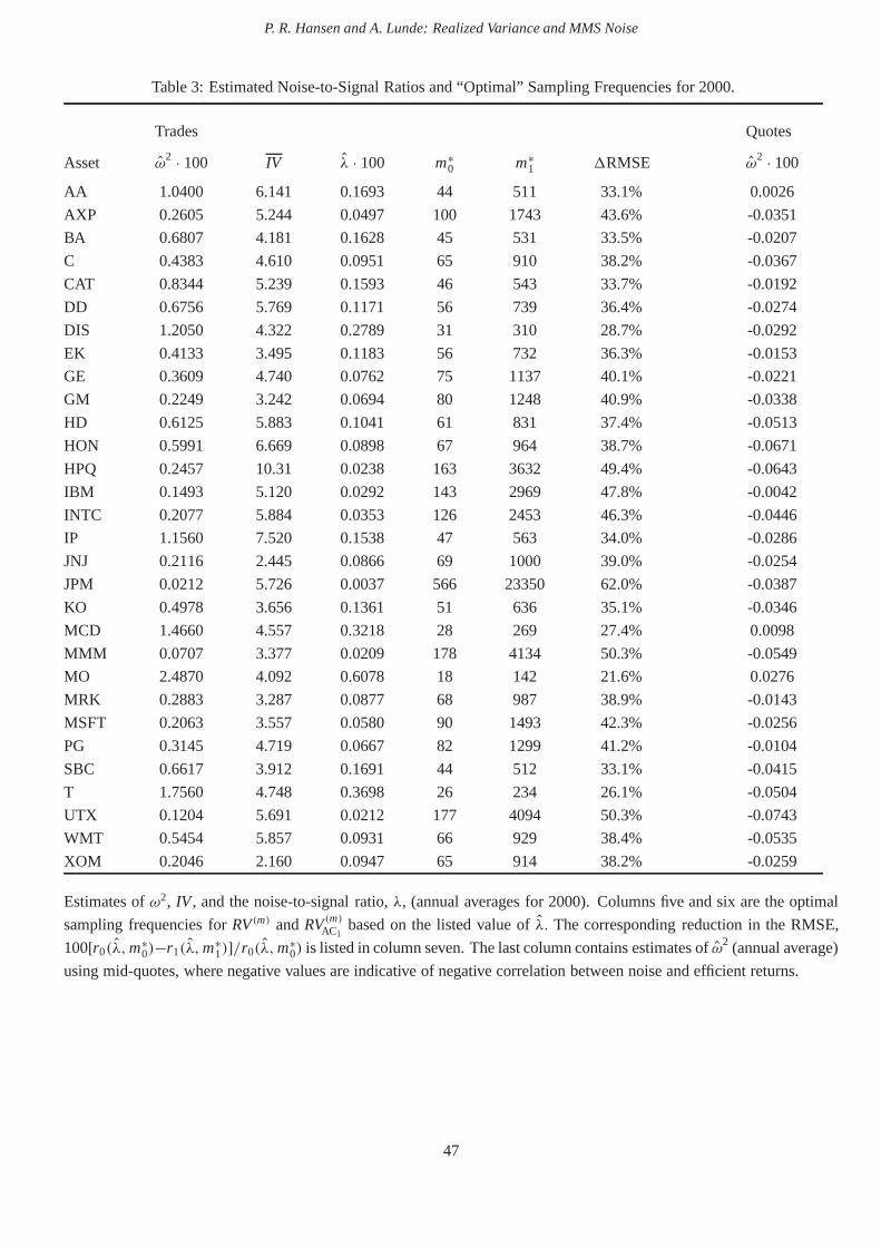
P. R. Hansen and A. Lunde: Realized Variance and MMS Noise
Table 3: Estimated Noise-to-Signal Ratios and “Optimal” Sampling Frequencies for 2000.
Trades Quotes
Asset ω2 · 100 IV λ · 100 m∗
0 m∗1 1RMSE ω
2 · 100
AA 1.0400 6.141 0.1693 44 511 33.1% 0.0026
AXP 0.2605 5.244 0.0497 100 1743 43.6% -0.0351
BA 0.6807 4.181 0.1628 45 531 33.5% -0.0207
C 0.4383 4.610 0.0951 65 910 38.2% -0.0367
CAT 0.8344 5.239 0.1593 46 543 33.7% -0.0192
DD 0.6756 5.769 0.1171 56 739 36.4% -0.0274
DIS 1.2050 4.322 0.2789 31 310 28.7% -0.0292
EK 0.4133 3.495 0.1183 56 732 36.3% -0.0153
GE 0.3609 4.740 0.0762 75 1137 40.1% -0.0221
GM 0.2249 3.242 0.0694 80 1248 40.9% -0.0338
HD 0.6125 5.883 0.1041 61 831 37.4% -0.0513
HON 0.5991 6.669 0.0898 67 964 38.7% -0.0671
HPQ 0.2457 10.31 0.0238 163 3632 49.4% -0.0643
IBM 0.1493 5.120 0.0292 143 2969 47.8% -0.0042
INTC 0.2077 5.884 0.0353 126 2453 46.3% -0.0446
IP 1.1560 7.520 0.1538 47 563 34.0% -0.0286
JNJ 0.2116 2.445 0.0866 69 1000 39.0% -0.0254
JPM 0.0212 5.726 0.0037 566 23350 62.0% -0.0387
KO 0.4978 3.656 0.1361 51 636 35.1% -0.0346
MCD 1.4660 4.557 0.3218 28 269 27.4% 0.0098
MMM 0.0707 3.377 0.0209 178 4134 50.3% -0.0549
MO 2.4870 4.092 0.6078 18 142 21.6% 0.0276
MRK 0.2883 3.287 0.0877 68 987 38.9% -0.0143
MSFT 0.2063 3.557 0.0580 90 1493 42.3% -0.0256
PG 0.3145 4.719 0.0667 82 1299 41.2% -0.0104
SBC 0.6617 3.912 0.1691 44 512 33.1% -0.0415
T 1.7560 4.748 0.3698 26 234 26.1% -0.0504
UTX 0.1204 5.691 0.0212 177 4094 50.3% -0.0743
WMT 0.5454 5.857 0.0931 66 929 38.4% -0.0535
XOM 0.2046 2.160 0.0947 65 914 38.2% -0.0259
Estimates ofω2, IV, and the noise-to-signal ratio,λ, (annual averages for 2000). Columns five and six are the optimal
sampling frequencies forRV(m) andRV(m)AC1based on the listed value ofλ. The corresponding reduction in the RMSE,
100[r0(λ,m∗0)−r1(λ,m∗
1)]/r0(λ,m∗0) is listed in column seven. The last column contains estimates ofω2 (annual average)
using mid-quotes, where negative values are indicative of negative correlation between noise and efficient returns.
47
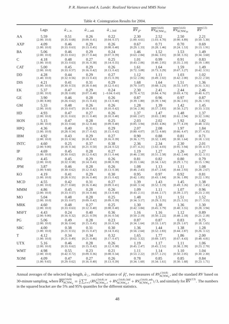
P. R. Hansen and A. Lunde: Realized Variance and MMS Noise
Table 4: Cointegration Results for 2004.
Lags α⊥,tr. α⊥,ask α⊥,bid RVp∗ RV(1tick)
ACNW15RV
(1tick)ACNW30
RV(13)
AA 5.59 0.51 0.26 0.22 2.30 2.52 2.50 2.21[2.00; 10.0] [0.35; 0.68] [0.09; 0.41] [0.04; 0.37] [1.00; 4.61] [1.03; 4.70] [0.90; 4.89] [0.50; 5.30]
AXP 4.09 0.46 0.29 0.26 0.67 0.71 0.70 0.69[1.00; 10.0] [0.33; 0.63] [0.13; 0.45] [0.08; 0.40] [0.29; 1.33] [0.28; 1.46] [0.24; 1.53] [0.13; 1.91]
BA 5.06 0.46 0.29 0.24 1.46 1.52 1.53 1.49[2.00; 10.0] [0.33; 0.61] [0.17; 0.44] [0.07; 0.39] [0.63; 2.84] [0.66; 3.01] [0.58; 3.35] [0.34; 3.60]
C 4.18 0.48 0.27 0.25 1.01 0.99 0.91 0.83[1.00; 10.0] [0.33; 0.63] [0.16; 0.38] [0.14; 0.35] [0.43; 2.06] [0.40; 2.05] [0.35; 2.10] [0.19; 1.80]
CAT 5.00 0.45 0.29 0.26 1.61 1.64 1.59 1.49[2.00; 10.0] [0.33; 0.57] [0.16; 0.42] [0.13; 0.42] [0.72; 3.08] [0.73; 3.29] [0.67; 3.27] [0.42; 3.51]
DD 4.28 0.44 0.29 0.27 1.12 1.11 1.03 1.02[1.40; 10.0] [0.32; 0.56] [0.13; 0.43] [0.15; 0.39] [0.52; 2.06] [0.49; 2.02] [0.42; 2.00] [0.22; 2.50]
DIS 4.21 0.41 0.31 0.29 1.68 1.64 1.51 1.36[1.00; 10.0] [0.30; 0.53] [0.18; 0.44] [0.12; 0.41] [0.70; 3.07] [0.68; 3.23] [0.55; 3.07] [0.31; 3.31]
EK 5.37 0.47 0.29 0.24 2.30 2.41 2.44 2.46[2.00; 10.0] [0.28; 0.69] [0.07; 0.48] [−0.04; 0.43] [0.79; 4.72] [0.84; 4.76] [0.69; 4.73] [0.40; 6.27]
GE 3.90 0.46 0.28 0.26 0.87 0.96 0.97 0.87[1.00; 8.00] [0.26; 0.62] [0.15; 0.43] [0.13; 0.40] [0.39; 1.80] [0.39; 1.94] [0.36; 2.01] [0.26; 1.93]
GM 5.33 0.48 0.26 0.26 1.28 1.39 1.42 1.45[2.00; 10.0] [0.33; 0.67] [0.10; 0.41] [0.10; 0.42] [0.54; 2.36] [0.57; 2.83] [0.50; 3.27] [0.33; 3.53]
HD 4.93 0.47 0.27 0.26 1.37 1.47 1.48 1.37[2.00; 10.0] [0.31; 0.63] [0.11; 0.40] [0.10; 0.40] [0.60; 2.67] [0.65; 2.80] [0.61; 2.94] [0.32; 3.06]
HON 5.15 0.47 0.28 0.25 2.03 2.02 1.92 1.82[1.00; 10.0] [0.33; 0.64] [0.12; 0.44] [0.09; 0.40] [0.85; 3.94] [0.83; 4.06] [0.77; 4.19] [0.48; 3.55]
HPQ 4.36 0.40 0.31 0.29 2.07 2.08 1.97 1.84[1.00; 10.0] [0.28; 0.54] [0.17; 0.42] [0.15; 0.42] [0.80; 4.07] [0.72; 4.60] [0.66; 4.47] [0.37; 4.35]
IBM 4.92 0.43 0.29 0.27 0.90 0.88 0.81 0.71[2.00; 10.0] [0.33; 0.56] [0.18; 0.42] [0.16; 0.39] [0.36; 1.77] [0.32; 1.69] [0.30; 1.64] [0.18; 1.53]
INTC 4.60 0.25 0.37 0.38 2.36 2.34 2.30 2.01[2.00; 9.00] [0.18; 0.34] [0.21; 0.50] [0.24; 0.52] [1.07; 4.21] [1.02; 4.03] [0.95; 3.94] [0.59; 4.17]
IP 4.69 0.45 0.28 0.27 1.19 1.27 1.26 1.27[1.00; 10.0] [0.30; 0.62] [0.12; 0.42] [0.11; 0.44] [0.46; 2.50] [0.51; 2.58] [0.42; 2.44] [0.32; 3.11]
JNJ 4.45 0.45 0.29 0.26 0.81 0.82 0.80 0.79[2.00; 10.0] [0.32; 0.58] [0.14; 0.43] [0.08; 0.39] [0.33; 1.66] [0.34; 1.62] [0.29; 1.71] [0.15; 1.96]
JPM 3.87 0.46 0.28 0.26 1.08 1.13 1.11 1.08[1.00; 9.60] [0.30; 0.62] [0.12; 0.42] [0.13; 0.38] [0.46; 2.43] [0.47; 2.64] [0.44; 2.93] [0.28; 2.67]
KO 4.19 0.41 0.29 0.30 0.95 0.97 0.92 0.81[1.00; 10.0] [0.28; 0.55] [0.16; 0.40] [0.15; 0.42] [0.42; 1.85] [0.43; 1.84] [0.36; 1.89] [0.22; 1.95]
MCD 4.55 0.42 0.31 0.27 1.39 1.43 1.45 1.38[1.00; 10.0] [0.27; 0.60] [0.16; 0.46] [0.09; 0.41] [0.60; 3.14] [0.52; 3.19] [0.49; 3.26] [0.32; 3.45]
MMM 4.86 0.45 0.28 0.26 1.09 1.11 1.07 0.96[2.00; 10.0] [0.33; 0.57] [0.14; 0.44] [0.13; 0.40] [0.43; 2.11] [0.44; 2.17] [0.39; 2.37] [0.23; 2.10]
MO 5.04 0.48 0.28 0.25 1.48 1.51 1.51 1.52[2.00; 10.0] [0.33; 0.67] [0.09; 0.42] [0.09; 0.39] [0.34; 3.17] [0.29; 3.35] [0.25; 3.31] [0.17; 3.55]
MRK 4.60 0.48 0.27 0.25 1.30 1.38 1.36 1.30[2.00; 10.0] [0.33; 0.63] [0.12; 0.40] [0.08; 0.40] [0.42; 3.84] [0.45; 3.79] [0.40; 3.55] [0.28; 3.94]
MSFT 4.43 0.24 0.40 0.36 1.16 1.16 1.12 0.89[2.00; 9.00] [0.16; 0.32] [0.21; 0.59] [0.16; 0.54] [0.50; 2.19] [0.50; 2.22] [0.48; 2.18] [0.21; 2.18]
PG 5.06 0.49 0.28 0.23 0.87 0.87 0.83 0.75[2.00; 10.0] [0.36; 0.64] [0.15; 0.45] [0.10; 0.34] [0.34; 1.64] [0.33; 1.67] [0.29; 1.67] [0.18; 1.65]
SBC 4.00 0.38 0.31 0.30 1.36 1.44 1.38 1.28[1.00; 10.0] [0.21; 0.55] [0.15; 0.47] [0.14; 0.45] [0.56; 2.64] [0.52; 2.83] [0.44; 2.87] [0.26; 3.12]
T 4.12 0.34 0.34 0.32 1.65 1.77 1.86 2.00[1.00; 10.0] [0.21; 0.49] [0.21; 0.46] [0.17; 0.47] [0.62; 3.32] [0.69; 3.87] [0.67; 4.43] [0.48; 4.81]
UTX 5.16 0.46 0.28 0.26 1.19 1.17 1.11 1.06[2.00; 10.0] [0.33; 0.62] [0.15; 0.42] [0.12; 0.38] [0.45; 2.47] [0.45; 2.51] [0.38; 2.39] [0.23; 2.70]
WMT 4.98 0.55 0.23 0.21 1.11 1.14 1.10 1.04[2.00; 10.0] [0.42; 0.72] [0.09; 0.36] [0.08; 0.34] [0.53; 2.22] [0.57; 2.21] [0.50; 2.05] [0.30; 2.30]
XOM 4.09 0.47 0.27 0.26 0.78 0.85 0.85 0.84[1.00; 9.65] [0.29; 0.62] [0.16; 0.40] [0.13; 0.39] [0.34; 1.60] [0.34; 1.61] [0.30; 1.68] [0.23; 1.71]
Annual averages of the selected lag-length,α⊥, realized variance ofp∗t , two measures ofRV(1tick)
ACNWq, and the standardRV based on
30-minute sampling, whereRV(1tick)
ACNWq≡ 1
n
∑nt=1(RV(1tick),tr
ACNWq,t+ RV(1tick),bid
ACNWq,t+ RV(1tick),ask
ACNWq,t)/3, and similarly forRV
(13). The numbers
in the squared bracket are the 5% and 95% quantiles for the different statistics.
48
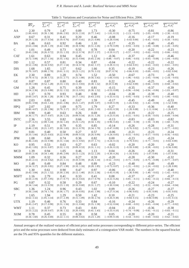
P. R. Hansen and A. Lunde: Realized Variance and MMS Noise
Table 5: Variations and Covariation for Noise and Efficient Price, 2004.
RVp∗∑
i e2i
tr. ∑i e2
i
ask ∑i e2
i
mid ∑i e2
i
bid ∑i ei y∗
itr. ∑
i ei y∗i
ask ∑i ei y∗
imid ∑
i ei y∗i
bid
AA 2.30 0.79 1.47 0.89 1.73 -0.30 -0.75 -0.81 -0.86[1.00; 4.61] [0.39; 1.58] [0.66; 2.92] [0.31; 2.10] [0.77; 3.41] [−1.01; 0.13] [−2.13; −0.05] [−2.05; −0.09] [−2.30; −0.12]
AXP 0.67 0.31 0.41 0.20 0.46 -0.08 -0.16 -0.17 -0.19[0.29; 1.33] [0.17; 0.54] [0.19; 0.76] [0.07; 0.41] [0.21; 0.89] [−0.28; 0.04] [−0.43; 0.00] [−0.45; −0.01] [−0.50; −0.01]
BA 1.46 0.63 0.92 0.46 1.10 -0.17 -0.35 -0.40 -0.45[0.63; 2.84] [0.28; 1.19] [0.42; 1.80] [0.18; 0.96] [0.51; 2.26] [−0.70; 0.09] [−0.93; −0.03] [−1.00; −0.08] [−1.20; −0.05]
C 1.01 0.49 0.73 0.35 0.78 0.04 -0.20 -0.22 -0.23[0.43; 2.06] [0.26; 0.72] [0.33; 1.33] [0.12; 0.74] [0.37; 1.57] [−0.19; 0.17] [−0.57; −0.01] [−0.62; −0.03] [−0.66; −0.02]
CAT 1.61 0.63 0.94 0.45 1.12 -0.36 -0.37 -0.42 -0.46[0.72; 3.08] [0.27; 1.16] [0.35; 1.92] [0.15; 0.84] [0.45; 2.18] [−0.88; −0.07] [−0.86; −0.03] [−0.93; −0.08] [−1.04; −0.05]
DD 1.12 0.57 0.81 0.34 0.87 -0.04 -0.22 -0.22 -0.22[0.52; 2.06] [0.34; 0.92] [0.37; 1.54] [0.14; 0.74] [0.42; 1.57] [−0.28; 0.11] [−0.64; 0.01] [−0.63; −0.02] [−0.61; −0.01]
DIS 1.68 1.65 1.57 0.62 1.66 0.35 -0.19 -0.23 -0.26[0.70; 3.07] [0.88; 2.70] [0.61; 3.11] [0.23; 1.21] [0.70; 3.13] [0.07; 0.74] [−0.66; 0.10] [−0.69; −0.01] [−0.82; 0.04]
EK 2.30 0.89 1.28 0.74 1.52 -0.50 -0.67 -0.73 -0.79[0.79; 4.72] [0.38; 1.72] [0.51; 2.77] [0.21; 1.80] [0.56; 3.42] [−1.66; 0.03] [−1.96; −0.02] [−2.05; −0.04] [−2.18; −0.03]
GE 0.87 0.87 0.80 0.40 0.83 0.22 -0.24 -0.25 -0.26[0.39; 1.80] [0.52; 1.28] [0.33; 1.55] [0.11; 0.83] [0.38; 1.52] [0.10; 0.38] [−0.62; 0.00] [−0.66; −0.03] [−0.68; −0.02]
GM 1.28 0.45 0.75 0.39 0.81 -0.15 -0.35 -0.37 -0.39[0.54; 2.36] [0.23; 0.80] [0.32; 1.52] [0.13; 0.91] [0.38; 1.52] [−0.53; 0.08] [−0.96; −0.04] [−0.94; −0.06] [−1.03; −0.07]
HD 1.37 0.70 0.93 0.48 0.98 -0.04 -0.38 -0.39 -0.40[0.60; 2.67] [0.36; 1.28] [0.38; 1.78] [0.17; 1.01] [0.43; 2.03] [−0.33; 0.15] [−0.95; −0.03] [−0.95; −0.05] [−1.00; −0.02]
HON 2.03 0.85 1.41 0.67 1.59 -0.17 -0.45 -0.49 -0.53[0.85; 3.94] [0.43; 1.43] [0.61; 2.86] [0.21; 1.47] [0.69; 3.07] [−0.69; 0.19] [−1.45; 0.02] [−1.42; −0.04] [−1.52; 0.00]
HPQ 2.07 2.02 1.69 0.75 1.79 0.27 -0.33 -0.36 -0.40[0.80; 4.07] [1.28; 2.96] [0.79; 3.17] [0.27; 1.42] [0.81; 3.10] [−0.03; 0.59] [−1.28; 0.08] [−1.11; 0.04] [−1.26; 0.07]
IBM 0.90 0.40 0.63 0.26 0.69 -0.03 -0.19 -0.22 -0.25[0.36; 1.77] [0.17; 0.67] [0.26; 1.23] [0.09; 0.54] [0.31; 1.29] [−0.23; 0.10] [−0.51; −0.01] [−0.59; −0.03] [−0.69; −0.04]
INTC 2.36 3.55 0.82 0.66 0.80 -0.13 -0.83 -0.83 -0.82[1.07; 4.21] [2.08; 5.24] [0.34; 1.43] [0.23; 1.25] [0.34; 1.35] [−0.96; 0.45] [−1.60; −0.30] [−1.59; −0.30] [−1.60; −0.29]
IP 1.19 0.51 0.79 0.35 0.85 -0.14 -0.26 -0.28 -0.31[0.46; 2.50] [0.21; 1.07] [0.30; 1.65] [0.11; 0.70] [0.34; 1.70] [−0.47; 0.09] [−0.76; 0.02] [−0.73; −0.01] [−0.77; −0.01]
JNJ 0.81 0.40 0.50 0.27 0.57 -0.06 -0.21 -0.23 -0.24[0.33; 1.66] [0.25; 0.63] [0.22; 0.98] [0.09; 0.53] [0.26; 0.99] [−0.24; 0.05] [−0.55; −0.01] [−0.57; −0.03] [−0.56; −0.02]
JPM 1.08 0.60 0.74 0.36 0.82 0.00 -0.23 -0.23 -0.24[0.46; 2.43] [0.33; 0.98] [0.31; 1.64] [0.11; 0.92] [0.37; 1.71] [−0.24; 0.13] [−0.79; 0.01] [−0.77; −0.01] [−0.83; 0.00]
KO 0.95 0.53 0.63 0.27 0.63 -0.02 -0.20 -0.20 -0.20[0.42; 1.85] [0.31; 0.87] [0.32; 1.13] [0.09; 0.53] [0.31; 1.11] [−0.26; 0.13] [−0.59; 0.00] [−0.58; −0.01] [−0.56; 0.00]
MCD 1.39 0.94 1.05 0.46 1.13 0.04 -0.26 -0.29 -0.31[0.60; 3.14] [0.54; 1.49] [0.46; 2.09] [0.15; 1.23] [0.52; 2.20] [−0.30; 0.26] [−1.16; 0.05] [−1.07; 0.00] [−1.07; 0.06]
MMM 1.09 0.32 0.56 0.27 0.59 -0.20 -0.28 -0.30 -0.32[0.43; 2.11] [0.14; 0.62] [0.23; 1.11] [0.10; 0.59] [0.26; 1.14] [−0.52; −0.01] [−0.71; −0.05] [−0.75; −0.08] [−0.77; −0.07]
MO 1.48 0.49 0.84 0.48 0.89 -0.23 -0.48 -0.49 -0.49[0.34; 3.17] [0.20; 0.81] [0.27; 1.90] [0.10; 1.16] [0.28; 1.85] [−0.73; 0.07] [−1.31; −0.01] [−1.24; −0.02] [−1.28; 0.00]
MRK 1.30 0.61 0.90 0.47 0.97 -0.06 -0.35 -0.37 -0.40[0.42; 3.84] [0.21; 1.52] [0.30; 2.50] [0.12; 1.40] [0.31; 2.36] [−0.43; 0.18] [−1.36; 0.00] [−1.40; −0.02] [−1.42; −0.01]
MSFT 1.16 2.79 0.41 0.33 0.41 0.08 -0.37 -0.37 -0.37[0.50; 2.19] [1.97; 3.95] [0.17; 0.77] [0.13; 0.63] [0.17; 0.79] [−0.22; 0.26] [−0.81; −0.11] [−0.82; −0.12] [−0.84; −0.13]
PG 0.87 0.32 0.58 0.29 0.67 -0.10 -0.22 -0.24 -0.27[0.34; 1.64] [0.13; 0.59] [0.23; 1.10] [0.10; 0.60] [0.31; 1.27] [−0.30; 0.04] [−0.52; −0.02] [−0.52; −0.04] [−0.64; −0.04]
SBC 1.36 1.24 0.96 0.43 1.02 0.09 -0.26 -0.27 -0.27[0.56; 2.64] [0.74; 1.74] [0.36; 1.77] [0.10; 0.95] [0.41; 1.99] [−0.27; 0.34] [−0.96; 0.05] [−0.91; 0.00] [−0.91; 0.03]
T 1.65 1.94 1.29 0.50 1.42 0.10 -0.21 -0.23 -0.25[0.62; 3.32] [1.05; 3.14] [0.57; 2.39] [0.15; 1.09] [0.58; 2.74] [−0.26; 0.38] [−0.84; 0.15] [−0.84; 0.08] [−1.01; 0.13]
UTX 1.19 0.46 0.76 0.33 0.84 -0.16 -0.24 -0.26 -0.29[0.45; 2.47] [0.17; 0.90] [0.31; 1.56] [0.11; 0.66] [0.35; 1.58] [−0.52; 0.04] [−0.68; −0.01] [−0.65; −0.04] [−0.77; −0.02]
WMT 1.11 0.37 0.73 0.43 0.81 -0.04 -0.33 -0.36 -0.38[0.53; 2.22] [0.18; 0.67] [0.38; 1.32] [0.20; 0.83] [0.41; 1.43] [−0.33; 0.10] [−0.74; −0.08] [−0.81; −0.11] [−0.83; −0.11]
XOM 0.78 0.45 0.55 0.28 0.58 0.05 -0.20 -0.20 -0.21[0.34; 1.60] [0.26; 0.69] [0.22; 1.11] [0.08; 0.63] [0.23; 1.20] [−0.09; 0.18] [−0.54; −0.01] [−0.60; −0.02] [−0.62; −0.02]
Annual averages of the realized variance of efficient price and noise processes corresponding to different price-series. The efficientprice and the noise processes were deduced from daily estimates of a cointegration VAR model. The numbers in the squared bracketare the 5% and 95% quantiles for the different statistics.
49
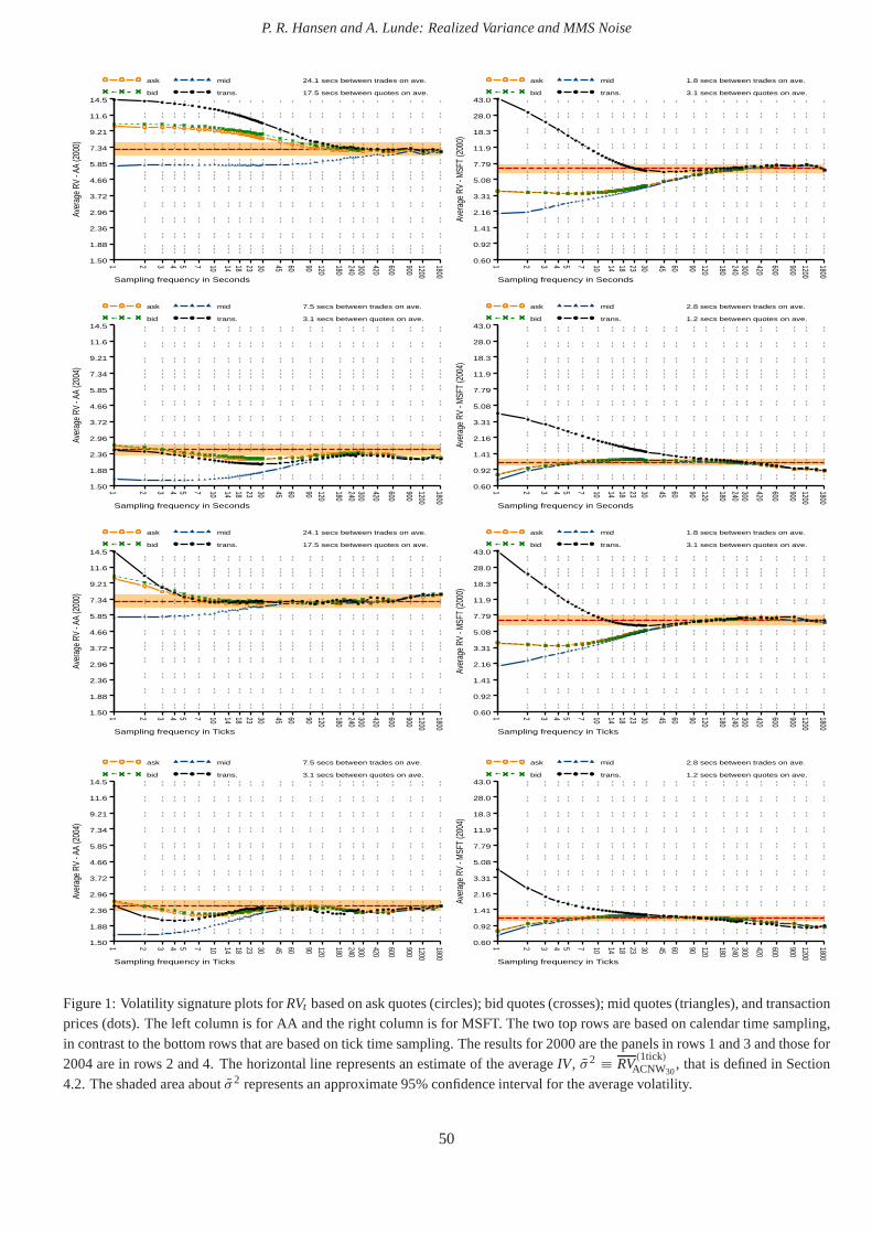
P. R. Hansen and A. Lunde: Realized Variance and MMS Noise
Aver
age
RV -
AA (2
000)
1.50
1.88
2.36
2.96
3.72
4.66
5.85
7.34
9.21
11.6
14.5
1 2 3 4 5 7 10 14 18 23 30 45 60 90 120
180
240300
420
600
900
1200
1800
Sampling frequency in Seconds
ask
bid
mid
trans.
24.1 secs between trades on ave.
17.5 secs between quotes on ave.
Aver
age
RV -
MSF
T (2
000)
0.60
0.92
1.41
2.16
3.31
5.08
7.79
11.9
18.3
28.0
43.0
1 2 3 4 5 7 10 14 18 23 30 45 60 90 120
180
240300
420
600
900
1200
1800
Sampling frequency in Seconds
ask
bid
mid
trans.
1.8 secs between trades on ave.
3.1 secs between quotes on ave.
Aver
age
RV -
AA (2
004)
1.50
1.88
2.36
2.96
3.72
4.66
5.85
7.34
9.21
11.6
14.5
1 2 3 4 5 7 10 14 18 23 30 45 60 90 120
180
240300
420
600
900
1200
1800
Sampling frequency in Seconds
ask
bid
mid
trans.
7.5 secs between trades on ave.
3.1 secs between quotes on ave.
Aver
age
RV -
MSF
T (2
004)
0.60
0.92
1.41
2.16
3.31
5.08
7.79
11.9
18.3
28.0
43.0
1 2 3 4 5 7 10 14 18 23 30 45 60 90 120
180
240300
420
600
900
1200
1800
Sampling frequency in Seconds
ask
bid
mid
trans.
2.8 secs between trades on ave.
1.2 secs between quotes on ave.
Aver
age
RV -
AA (2
000)
1.50
1.88
2.36
2.96
3.72
4.66
5.85
7.34
9.21
11.6
14.5
1 2 3 4 5 7 10 14 18 23 30 45 60 90 120
180
240300
420
600
900
1200
1800
Sampling frequency in Ticks
ask
bid
mid
trans.
24.1 secs between trades on ave.
17.5 secs between quotes on ave.
Aver
age
RV -
MSF
T (2
000)
0.60
0.92
1.41
2.16
3.31
5.08
7.79
11.9
18.3
28.0
43.0
1 2 3 4 5 7 10 14 18 23 30 45 60 90 120
180
240300
420
600
900
1200
1800
Sampling frequency in Ticks
ask
bid
mid
trans.
1.8 secs between trades on ave.
3.1 secs between quotes on ave.
Aver
age
RV -
AA (2
004)
1.50
1.88
2.36
2.96
3.72
4.66
5.85
7.34
9.21
11.6
14.5
1 2 3 4 5 7 10 14 18 23 30 45 60 90 120
180
240300
420
600
900
1200
1800
Sampling frequency in Ticks
ask
bid
mid
trans.
7.5 secs between trades on ave.
3.1 secs between quotes on ave.
Aver
age
RV -
MSF
T (2
004)
0.60
0.92
1.41
2.16
3.31
5.08
7.79
11.9
18.3
28.0
43.0
1 2 3 4 5 7 10 14 18 23 30 45 60 90 120
180
240300
420
600
900
1200
1800
Sampling frequency in Ticks
ask
bid
mid
trans.
2.8 secs between trades on ave.
1.2 secs between quotes on ave.
Figure 1: Volatility signature plots forRVt based on ask quotes (circles); bid quotes (crosses); mid quotes (triangles), and transactionprices (dots). The left column is for AA and the right column is for MSFT. The two top rows are based on calendar time sampling,in contrast to the bottom rows that are based on tick time sampling. The results for 2000 are the panels in rows 1 and 3 and those for2004 are in rows 2 and 4. The horizontal line represents an estimate of the averageIV, σ 2 ≡ RV
(1tick)ACNW30
, that is defined in Section4.2. The shaded area aboutσ 2 represents an approximate 95% confidence interval for the average volatility.
50
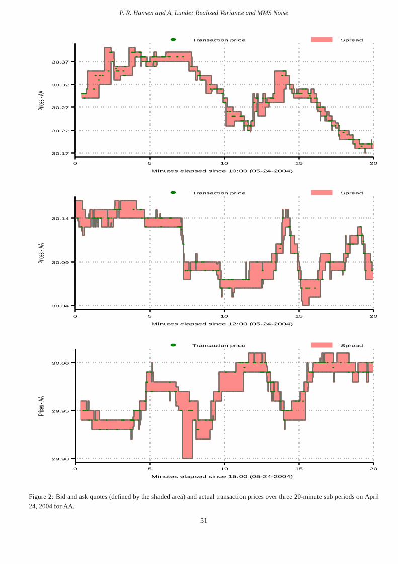
P. R. Hansen and A. Lunde: Realized Variance and MMS Noise
Transaction price SpreadPri
ces - A
A
0 5 10 15 20
Minutes elapsed since 10:00 (05-24-2004)
30.17
30.22
30.27
30.32
30.37
Transaction price Spread
Prices
- AA
0 5 10 15 20
Minutes elapsed since 12:00 (05-24-2004)
30.04
30.09
30.14
Transaction price Spread
Prices
- AA
0 5 10 15 20
Minutes elapsed since 15:00 (05-24-2004)
29.90
29.95
30.00
Figure 2: Bid and ask quotes (defined by the shaded area) and actual transaction prices over three 20-minute sub periods onApril24, 2004 for AA.
51
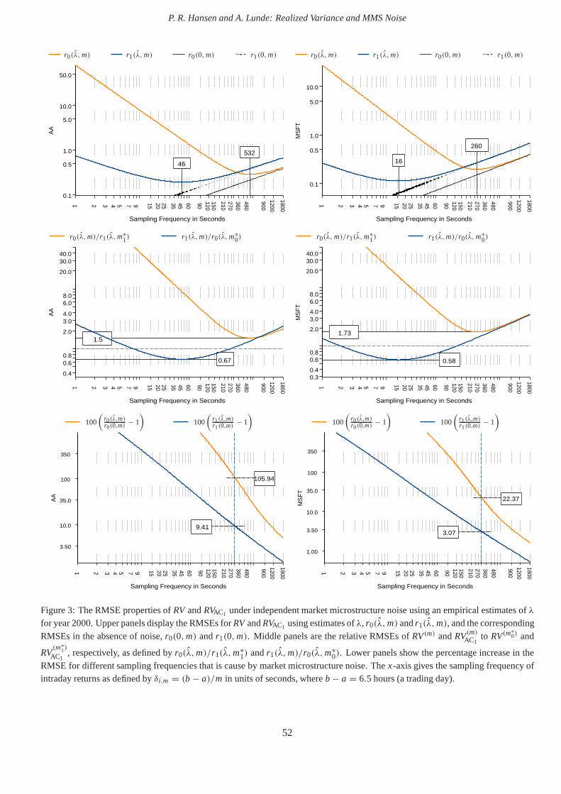
P. R. Hansen and A. Lunde: Realized Variance and MMS Noise
AA
0.1
0.5
1.0
5.0
10.0
50.0
1 2 3 4 5 7 9 15 20 25 35 45 60 90120150
210270360
480
900
1200
1800
Sampling Frequency in Seconds
532
46
r0(λ,m) r1(λ,m) r0(0,m) r1(0,m)
MS
FT
0.1
0.5
1.0
5.0
10.0
1 2 3 4 5 7 9 15 20 25 35 45 60 90120150
210270360
480
900
1200
1800
Sampling Frequency in Seconds
260
16
r0(λ,m) r1(λ,m) r0(0,m) r1(0,m)A
A
0.4
0.60.8
2.0
3.04.0
6.08.0
20.0
30.040.0
0.67
1.5
1 2 3 4 5 7 9 15 20 25 35 45 60 90120150
210270360
480
900
1200
1800
Sampling Frequency in Seconds
r0(λ,m)/r1(λ,m∗1) r1(λ,m)/r0(λ,m
∗0)
MS
FT
0.30.4
0.60.8
2.0
3.04.0
6.08.0
20.0
30.040.0
0.58
1.73
1 2 3 4 5 7 9 15 20 25 35 45 60 90120150
210270360
480
900
1200
1800
Sampling Frequency in Seconds
r0(λ,m)/r1(λ,m∗1) r1(λ,m)/r0(λ,m
∗0)
AA
105.94
9.41
3.50
10.0
35.0
100
350
1 2 3 4 5 7 9 15 20 25 35 45 60 90120150
210270360480
900
1200
1800
Sampling Frequency in Seconds
100
(r0(λ,m)r0(0,m)
− 1
)100
(r1(λ,m)r1(0,m)
− 1
)
MS
FT
22.37
3.07
1.00
3.50
10.0
35.0
100
350
1 2 3 4 5 7 9 15 20 25 35 45 60 90120150
210270360480
900
1200
1800
Sampling Frequency in Seconds
100
(r0(λ,m)r0(0,m)
− 1
)100
(r1(λ,m)r1(0,m)
− 1
)
Figure 3: The RMSE properties ofRV andRVAC1 under independent market microstructure noise using an empirical estimates ofλfor year 2000. Upper panels display the RMSEs forRVandRVAC1 using estimates ofλ, r0(λ,m) andr1(λ,m), and the correspondingRMSEs in the absence of noise,r0(0,m) andr1(0,m). Middle panels are the relative RMSEs ofRV(m) andRV(m)AC1
to RV(m∗0) and
RV(m∗
1)
AC1, respectively, as defined byr0(λ,m)/r1(λ,m∗
1) andr1(λ,m)/r0(λ,m∗0). Lower panels show the percentage increase in the
RMSE for different sampling frequencies that is cause by market microstructure noise. Thex-axis gives the sampling frequency ofintraday returns as defined byδi,m = (b − a)/m in units of seconds, whereb − a = 6.5 hours (a trading day).
52
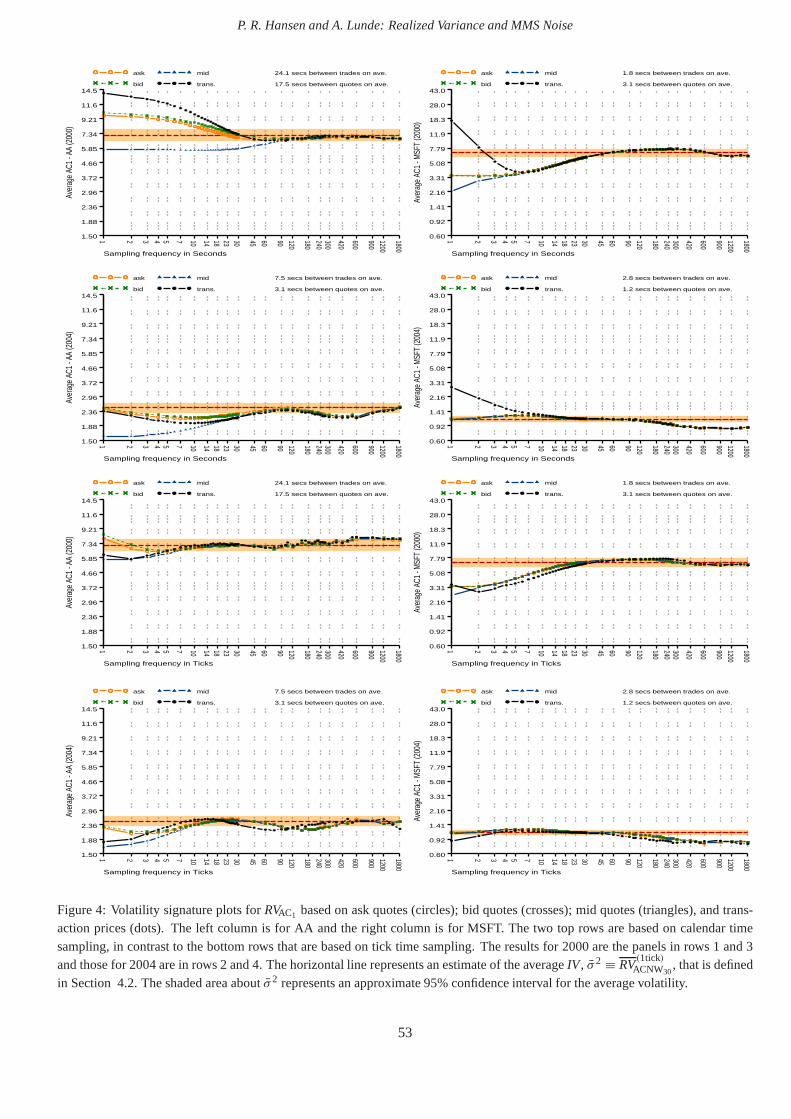
P. R. Hansen and A. Lunde: Realized Variance and MMS Noise
Aver
age
AC1
- AA
(200
0)
1.50
1.88
2.36
2.96
3.72
4.66
5.85
7.34
9.21
11.6
14.5
1 2 3 4 5 7 10 14 18 23 30 45 60 90 120
180
240300
420
600
900
1200
1800
Sampling frequency in Seconds
ask
bid
mid
trans.
24.1 secs between trades on ave.
17.5 secs between quotes on ave.
Aver
age
AC1
- MSF
T (2
000)
0.60
0.92
1.41
2.16
3.31
5.08
7.79
11.9
18.3
28.0
43.0
1 2 3 4 5 7 10 14 18 23 30 45 60 90 120
180
240300
420
600
900
1200
1800
Sampling frequency in Seconds
ask
bid
mid
trans.
1.8 secs between trades on ave.
3.1 secs between quotes on ave.
Aver
age
AC1
- AA
(200
4)
1.50
1.88
2.36
2.96
3.72
4.66
5.85
7.34
9.21
11.6
14.5
1 2 3 4 5 7 10 14 18 23 30 45 60 90 120
180
240300
420
600
900
1200
1800
Sampling frequency in Seconds
ask
bid
mid
trans.
7.5 secs between trades on ave.
3.1 secs between quotes on ave.
Aver
age
AC1
- MSF
T (2
004)
0.60
0.92
1.41
2.16
3.31
5.08
7.79
11.9
18.3
28.0
43.0
1 2 3 4 5 7 10 14 18 23 30 45 60 90 120
180
240300
420
600
900
1200
1800
Sampling frequency in Seconds
ask
bid
mid
trans.
2.8 secs between trades on ave.
1.2 secs between quotes on ave.
Aver
age
AC1
- AA
(200
0)
1.50
1.88
2.36
2.96
3.72
4.66
5.85
7.34
9.21
11.6
14.5
1 2 3 4 5 7 10 14 18 23 30 45 60 90 120
180
240300
420
600
900
1200
1800
Sampling frequency in Ticks
ask
bid
mid
trans.
24.1 secs between trades on ave.
17.5 secs between quotes on ave.
Aver
age
AC1
- MSF
T (2
000)
0.60
0.92
1.41
2.16
3.31
5.08
7.79
11.9
18.3
28.0
43.0
1 2 3 4 5 7 10 14 18 23 30 45 60 90 120
180
240300
420
600
900
1200
1800
Sampling frequency in Ticks
ask
bid
mid
trans.
1.8 secs between trades on ave.
3.1 secs between quotes on ave.
Aver
age
AC1
- AA
(200
4)
1.50
1.88
2.36
2.96
3.72
4.66
5.85
7.34
9.21
11.6
14.5
1 2 3 4 5 7 10 14 18 23 30 45 60 90 120
180
240300
420
600
900
1200
1800
Sampling frequency in Ticks
ask
bid
mid
trans.
7.5 secs between trades on ave.
3.1 secs between quotes on ave.
Aver
age
AC1
- MSF
T (2
004)
0.60
0.92
1.41
2.16
3.31
5.08
7.79
11.9
18.3
28.0
43.0
1 2 3 4 5 7 10 14 18 23 30 45 60 90 120
180
240300
420
600
900
1200
1800
Sampling frequency in Ticks
ask
bid
mid
trans.
2.8 secs between trades on ave.
1.2 secs between quotes on ave.
Figure 4: Volatility signature plots forRVAC1 based on ask quotes (circles); bid quotes (crosses); mid quotes (triangles), and trans-action prices (dots). The left column is for AA and the right column is for MSFT. The two top rows are based on calendar timesampling, in contrast to the bottom rows that are based on tick time sampling. The results for 2000 are the panels in rows 1 and 3and those for 2004 are in rows 2 and 4. The horizontal line represents an estimate of the averageIV, σ 2 ≡ RV
(1tick)ACNW30
, that is definedin Section 4.2. The shaded area aboutσ 2 represents an approximate 95% confidence interval for the average volatility.
53
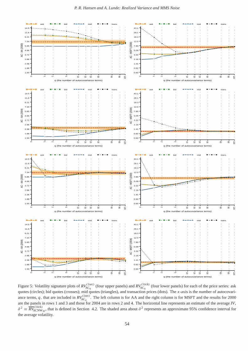
P. R. Hansen and A. Lunde: Realized Variance and MMS Noise
AC -
AA (2
000)
1.50
1.88
2.36
2.96
3.72
4.66
5.85
7.34
9.21
11.6
14.5
0 1 2 5 10 15 20 30 60 90 120
q (the number of autocovariance terms)
ask bid mid trans.
AC -
MSF
T (2
000)
0.60
0.92
1.41
2.16
3.32
5.09
7.80
12.0
18.3
28.1
43.1
0 1 2 5 10 15 20 30 60 90 120
q (the number of autocovariance terms)
ask bid mid trans.AC
- AA
(200
4)
1.50
1.88
2.36
2.96
3.72
4.66
5.85
7.34
9.21
11.6
14.5
0 1 2 5 10 15 20 30 60 90 120
q (the number of autocovariance terms)
ask bid mid trans.
AC -
MSF
T (2
004)
0.60
0.92
1.41
2.16
3.32
5.09
7.80
12.0
18.3
28.1
43.1
0 1 2 5 10 15 20 30 60 90 120
q (the number of autocovariance terms)
ask bid mid trans.
AC -
AA (2
000)
1.50
1.88
2.36
2.96
3.72
4.66
5.85
7.34
9.21
11.6
14.5
0 1 2 5 10 15 20 30 60 90 120
q (the number of autocovariance terms)
ask bid mid trans.
AC -
MSF
T (2
000)
0.60
0.92
1.41
2.16
3.32
5.09
7.80
12.0
18.3
28.1
43.1
0 1 2 5 10 15 20 30 60 90 120
q (the number of autocovariance terms)
ask bid mid trans.
AC -
AA (2
004)
1.50
1.88
2.36
2.96
3.72
4.66
5.85
7.34
9.21
11.6
14.5
0 1 2 5 10 15 20 30 60 90 120
q (the number of autocovariance terms)
ask bid mid trans.
AC -
MSF
T (2
004)
0.60
0.92
1.41
2.16
3.32
5.09
7.80
12.0
18.3
28.1
43.1
0 1 2 5 10 15 20 30 60 90 120
q (the number of autocovariance terms)
ask bid mid trans.
Figure 5: Volatility signature plots ofRV(1sec)ACq
(four upper panels) andRV(1tick)ACq
(four lower panels) for each of the price series: askquotes (circles); bid quotes (crosses); mid quotes (triangles), and transaction prices (dots). Thex-axis is the number of autocovari-ance terms,q, that are included inRV(1sec)
ACq. The left column is for AA and the right column is for MSFT and the results for 2000
are the panels in rows 1 and 3 and those for 2004 are in rows 2 and4. The horizontal line represents an estimate of the averageIV,σ 2 ≡ RV
(1tick)ACNW30
, that is defined in Section 4.2. The shaded area aboutσ 2 represents an approximate 95% confidence interval forthe average volatility.
54
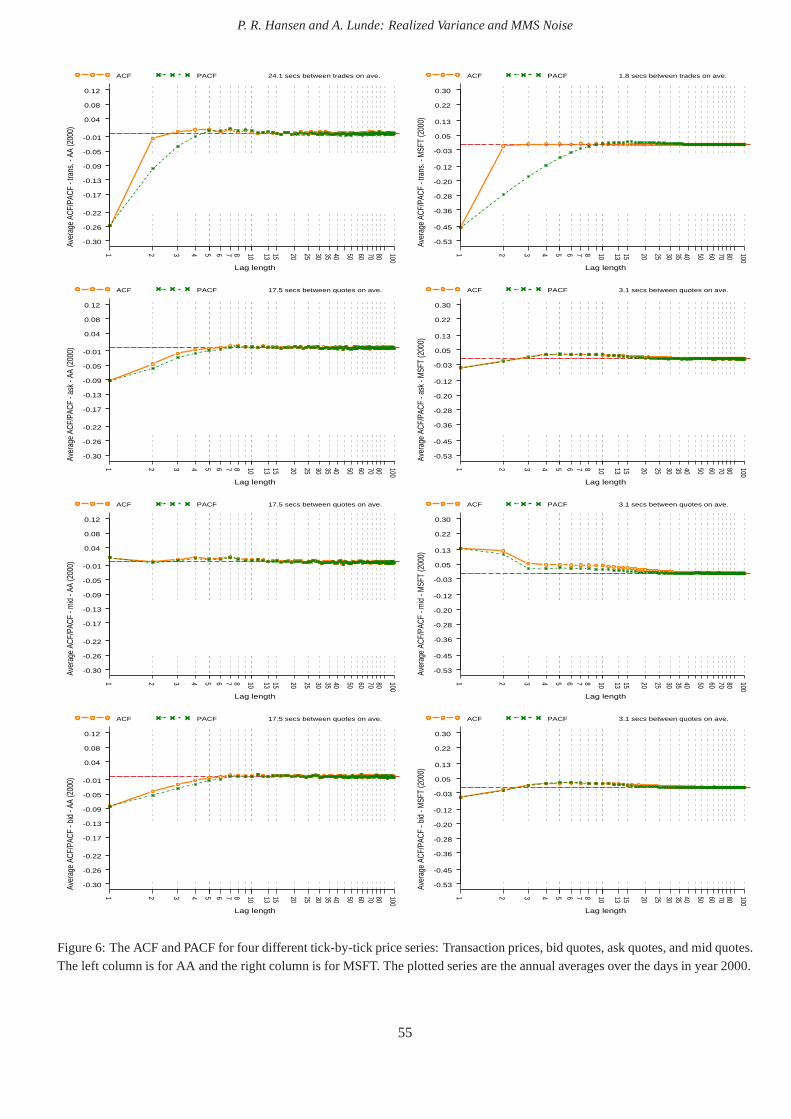
P. R. Hansen and A. Lunde: Realized Variance and MMS Noise
Aver
age
ACF/
PACF
- tra
ns. -
AA
(200
0)
-0.30
-0.26
-0.22
-0.17
-0.13
-0.09
-0.05
-0.01
0.04
0.08
0.12
1 2 3 4 5 6 7 8 10 13 15 20 25 30 35 40 50 60 70 80 100
Lag length
ACF PACF 24.1 secs between trades on ave.
Aver
age
ACF/
PACF
- tra
ns. -
MSF
T (2
000)
-0.53
-0.45
-0.36
-0.28
-0.20
-0.12
-0.03
0.05
0.13
0.22
0.30
1 2 3 4 5 6 7 8 10 13 15 20 25 30 35 40 50 60 70 80 100
Lag length
ACF PACF 1.8 secs between trades on ave.Av
erag
e AC
F/PA
CF -
ask
- AA
(200
0)
-0.30
-0.26
-0.22
-0.17
-0.13
-0.09
-0.05
-0.01
0.04
0.08
0.12
1 2 3 4 5 6 7 8 10 13 15 20 25 30 35 40 50 60 70 80 100
Lag length
ACF PACF 17.5 secs between quotes on ave.
Aver
age
ACF/
PACF
- as
k - M
SFT
(200
0)
-0.53
-0.45
-0.36
-0.28
-0.20
-0.12
-0.03
0.05
0.13
0.22
0.30
1 2 3 4 5 6 7 8 10 13 15 20 25 30 35 40 50 60 70 80 100
Lag length
ACF PACF 3.1 secs between quotes on ave.
Aver
age
ACF/
PACF
- m
id -
AA (2
000)
-0.30
-0.26
-0.22
-0.17
-0.13
-0.09
-0.05
-0.01
0.04
0.08
0.12
1 2 3 4 5 6 7 8 10 13 15 20 25 30 35 40 50 60 70 80 100
Lag length
ACF PACF 17.5 secs between quotes on ave.
Aver
age
ACF/
PACF
- m
id -
MSF
T (2
000)
-0.53
-0.45
-0.36
-0.28
-0.20
-0.12
-0.03
0.05
0.13
0.22
0.30
1 2 3 4 5 6 7 8 10 13 15 20 25 30 35 40 50 60 70 80 100
Lag length
ACF PACF 3.1 secs between quotes on ave.
Aver
age
ACF/
PACF
- bi
d - A
A (2
000)
-0.30
-0.26
-0.22
-0.17
-0.13
-0.09
-0.05
-0.01
0.04
0.08
0.12
1 2 3 4 5 6 7 8 10 13 15 20 25 30 35 40 50 60 70 80 100
Lag length
ACF PACF 17.5 secs between quotes on ave.
Aver
age
ACF/
PACF
- bi
d - M
SFT
(200
0)
-0.53
-0.45
-0.36
-0.28
-0.20
-0.12
-0.03
0.05
0.13
0.22
0.30
1 2 3 4 5 6 7 8 10 13 15 20 25 30 35 40 50 60 70 80 100
Lag length
ACF PACF 3.1 secs between quotes on ave.
Figure 6: The ACF and PACF for four different tick-by-tick price series: Transaction prices, bid quotes, ask quotes, andmid quotes.The left column is for AA and the right column is for MSFT. The plotted series are the annual averages over the days in year 2000.
55
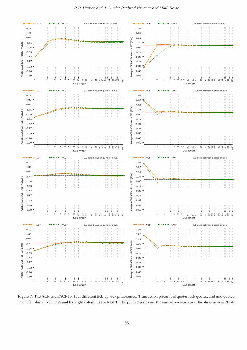
P. R. Hansen and A. Lunde: Realized Variance and MMS Noise
Aver
age
ACF/
PACF
- tra
ns. -
AA
(200
4)
-0.30
-0.26
-0.22
-0.17
-0.13
-0.09
-0.05
-0.01
0.04
0.08
0.12
1 2 3 4 5 6 7 8 10 13 15 20 25 30 35 40 50 60 70 80 100
Lag length
ACF PACF 7.5 secs between trades on ave.
Aver
age
ACF/
PACF
- tra
ns. -
MSF
T (2
004)
-0.53
-0.45
-0.36
-0.28
-0.20
-0.12
-0.03
0.05
0.13
0.22
0.30
1 2 3 4 5 6 7 8 10 13 15 20 25 30 35 40 50 60 70 80 100
Lag length
ACF PACF 2.8 secs between trades on ave.Av
erag
e AC
F/PA
CF -
ask
- AA
(200
4)
-0.30
-0.26
-0.22
-0.17
-0.13
-0.09
-0.05
-0.01
0.04
0.08
0.12
1 2 3 4 5 6 7 8 10 13 15 20 25 30 35 40 50 60 70 80 100
Lag length
ACF PACF 3.1 secs between quotes on ave.
Aver
age
ACF/
PACF
- as
k - M
SFT
(200
4)
-0.53
-0.45
-0.36
-0.28
-0.20
-0.12
-0.03
0.05
0.13
0.22
0.30
1 2 3 4 5 6 7 8 10 13 15 20 25 30 35 40 50 60 70 80 100
Lag length
ACF PACF 1.2 secs between quotes on ave.
Aver
age
ACF/
PACF
- m
id -
AA (2
004)
-0.30
-0.26
-0.22
-0.17
-0.13
-0.09
-0.05
-0.01
0.04
0.08
0.12
1 2 3 4 5 6 7 8 10 13 15 20 25 30 35 40 50 60 70 80 100
Lag length
ACF PACF 3.1 secs between quotes on ave.
Aver
age
ACF/
PACF
- m
id -
MSF
T (2
004)
-0.53
-0.45
-0.36
-0.28
-0.20
-0.12
-0.03
0.05
0.13
0.22
0.30
1 2 3 4 5 6 7 8 10 13 15 20 25 30 35 40 50 60 70 80 100
Lag length
ACF PACF 1.2 secs between quotes on ave.
Aver
age
ACF/
PACF
- bi
d - A
A (2
004)
-0.30
-0.26
-0.22
-0.17
-0.13
-0.09
-0.05
-0.01
0.04
0.08
0.12
1 2 3 4 5 6 7 8 10 13 15 20 25 30 35 40 50 60 70 80 100
Lag length
ACF PACF 3.1 secs between quotes on ave.
Aver
age
ACF/
PACF
- bi
d - M
SFT
(200
4)
-0.53
-0.45
-0.36
-0.28
-0.20
-0.12
-0.03
0.05
0.13
0.22
0.30
1 2 3 4 5 6 7 8 10 13 15 20 25 30 35 40 50 60 70 80 100
Lag length
ACF PACF 1.2 secs between quotes on ave.
Figure 7: The ACF and PACF for four different tick-by-tick price series: Transaction prices, bid quotes, ask quotes, andmid quotes.The left column is for AA and the right column is for MSFT. The plotted series are the annual averages over the days in year 2004.
56
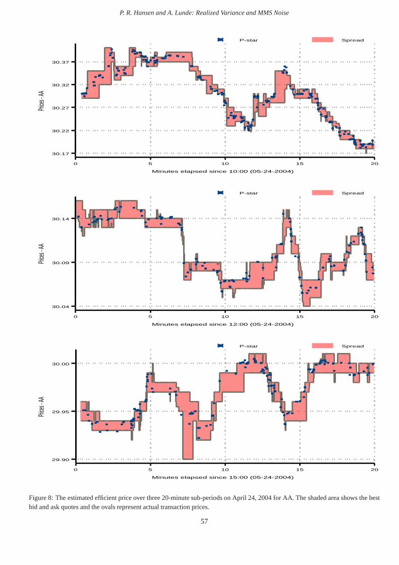
P. R. Hansen and A. Lunde: Realized Variance and MMS Noise
P-star SpreadPri
ces - A
A
0 5 10 15 20
Minutes elapsed since 10:00 (05-24-2004)
30.17
30.22
30.27
30.32
30.37
P-star Spread
Prices
- AA
0 5 10 15 20
Minutes elapsed since 12:00 (05-24-2004)
30.04
30.09
30.14
P-star Spread
Prices
- AA
0 5 10 15 20
Minutes elapsed since 15:00 (05-24-2004)
29.90
29.95
30.00
Figure 8: The estimated efficient price over three 20-minutesub-periods on April 24, 2004 for AA. The shaded area shows the bestbid and ask quotes and the ovals represent actual transaction prices.
57
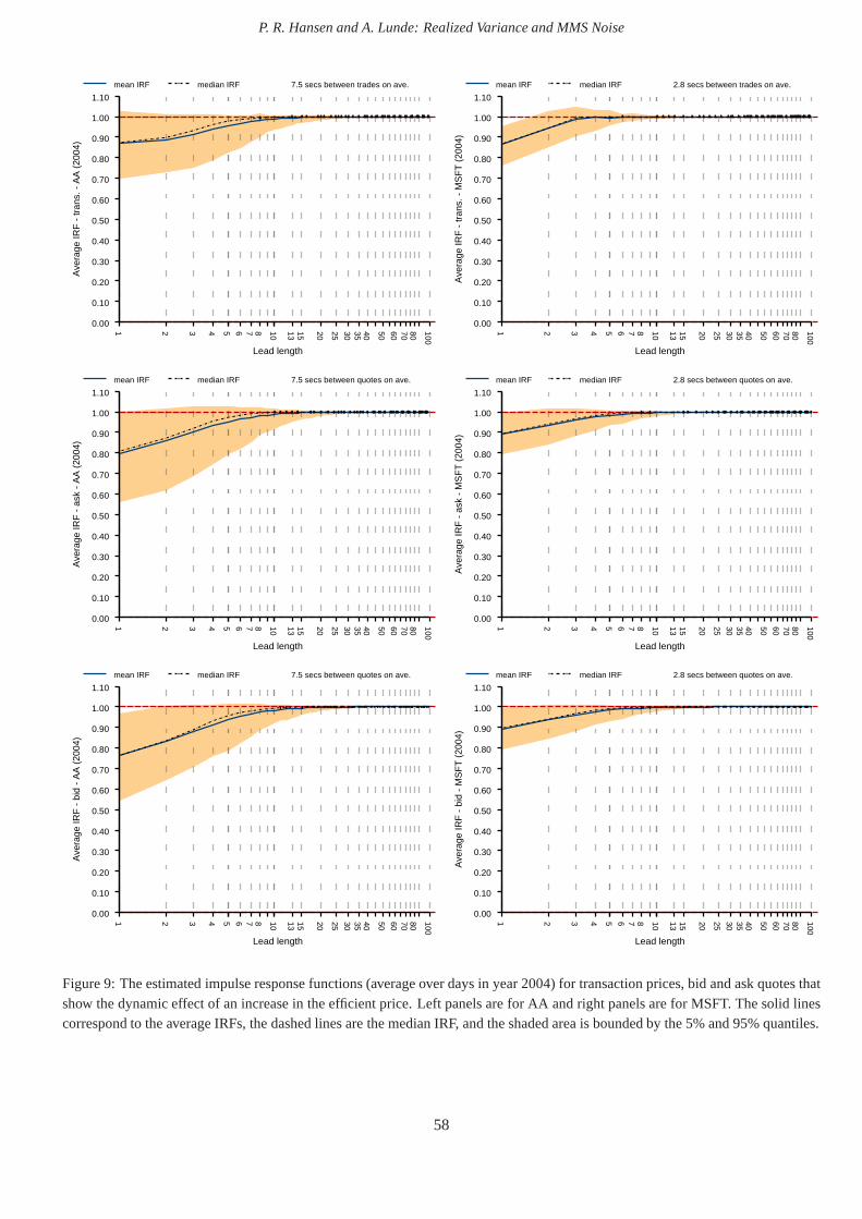
P. R. Hansen and A. Lunde: Realized Variance and MMS Noise
Ave
rage
IRF
- tr
ans.
- A
A (
2004
)
0.00
0.10
0.20
0.30
0.40
0.50
0.60
0.70
0.80
0.90
1.00
1.10
1 2 3 4 5 6 7 8 10 13 15 20 25 30 35 40 50 60 70 80 100
Lead length
mean IRF median IRF 7.5 secs between trades on ave.
Ave
rage
IRF
- tr
ans.
- M
SF
T (
2004
)
0.00
0.10
0.20
0.30
0.40
0.50
0.60
0.70
0.80
0.90
1.00
1.10
1 2 3 4 5 6 7 8 10 13 15 20 25 30 35 40 50 60 70 80 100
Lead length
mean IRF median IRF 2.8 secs between trades on ave.A
vera
ge IR
F -
ask
- A
A (
2004
)
0.00
0.10
0.20
0.30
0.40
0.50
0.60
0.70
0.80
0.90
1.00
1.10
1 2 3 4 5 6 7 8 10 13 15 20 25 30 35 40 50 60 70 80 100
Lead length
mean IRF median IRF 7.5 secs between quotes on ave.
Ave
rage
IRF
- a
sk -
MS
FT
(20
04)
0.00
0.10
0.20
0.30
0.40
0.50
0.60
0.70
0.80
0.90
1.00
1.10
1 2 3 4 5 6 7 8 10 13 15 20 25 30 35 40 50 60 70 80 100
Lead length
mean IRF median IRF 2.8 secs between quotes on ave.
Ave
rage
IRF
- b
id -
AA
(20
04)
0.00
0.10
0.20
0.30
0.40
0.50
0.60
0.70
0.80
0.90
1.00
1.10
1 2 3 4 5 6 7 8 10 13 15 20 25 30 35 40 50 60 70 80 100
Lead length
mean IRF median IRF 7.5 secs between quotes on ave.
Ave
rage
IRF
- b
id -
MS
FT
(20
04)
0.00
0.10
0.20
0.30
0.40
0.50
0.60
0.70
0.80
0.90
1.00
1.10
1 2 3 4 5 6 7 8 10 13 15 20 25 30 35 40 50 60 70 80 100
Lead length
mean IRF median IRF 2.8 secs between quotes on ave.
Figure 9: The estimated impulse response functions (average over days in year 2004) for transaction prices, bid and ask quotes thatshow the dynamic effect of an increase in the efficient price.Left panels are for AA and right panels are for MSFT. The solidlinescorrespond to the average IRFs, the dashed lines are the median IRF, and the shaded area is bounded by the 5% and 95% quantiles.
58