Embed Size (px)
Citation preview
REALIZING FRACTIONAL DERIVATIVES OF ELEMENTARY AND COMPOSITE
FUNCTIONS THROUGH THE GENERALIZED EULER’S INTEGRAL
TRANSFORM AND INTEGER DERIVATIVE SERIES: BUILDING
THE MATHEMATICAL FRAMEWORK TO MODEL THE
FRACTIONAL SCHRODINGER EQUATION IN
FRACTIONAL SPACETIME
by
Anastasia Gladkina
© Copyright by Anastasia Gladkina, 2018
All Rights Reserved
A thesis submitted to the Faculty and the Board of Trustees of the Colorado School of Mines
in partial fulfillment of the requirements for the degree of Master of Science (Applied Physics).
Golden, Colorado
Date
Signed:Anastasia Gladkina
Signed:Dr. Lincoln D. Carr
Thesis Advisor
Signed:Dr. Gavriil Shchedrin
Thesis Advisor
Golden, Colorado
Date
Signed:Dr. rer. nat. Uwe Greife
Professor and HeadDepartment of Physics
ii
ABSTRACT
Since the engenderment of fractional derivatives in 1695 as a continuous transformation be-
tween integer order derivatives, the physical applicability of fractional derivatives has been ques-
tioned. While it is true that they share a set of distinguishing characteristics, no two fractional
derivatives are alike. With each definition mathematically valid but results of one fractional deriva-
tive inconsistent with another, the theory of fractional calculus slowly evolved to create an inter-
connected web of ideas, limits, and insight. In time fractional derivatives came to be recognized
as a powerful and ubiquitous tool. For example, fractional derivatives easily characterize the dy-
namics of anomalous diffusion in experimental settings where particles are allowed to jump farther
than in a Gaussian-distributed random walk. With experimental evidence confirming the physical
realization of fractional derivatives, the emphasis in research has been on developing both analytic
and numerical tools to treat specific problems in fractional calculus.
Similarly in this work we approach fractional derivatives from analytic and numerical perspec-
tives. From large classical systems where it is easy to see the contribution of fractional deriva-
tives we transition to fractional quantum mechanics, where the physical interpretation of fractional
derivatives becomes more ambiguous. We concentrate on deriving the fractional Schrodinger equa-
tion via the Feynman path integral, under the assumption that space and time coordinates scale at
different rates. This generalization is particularly useful for quantum systems where the under-
lying potential is characterized by a scaling relation. Scaling relations common to dynamics on
self-similar geometries do not themselves justify the replacement of integer order derivatives by
fractional derivatives. Instead, we seek to describe the evolution of a quantum particle in a particu-
lar class of nonlocal potentials, where to realize the kinetic energy of a particle we need to consider
a large finite neighborhood. We study symmetry properties of the fractional Schrodinger equation
and conclude that only a small subset of fractional derivatives ensures the Hamiltonian is parity-
and time-reversal symmetric.
iii
To coalesce several fractional derivatives and further emphasize the similarities between them,
we cast the finite difference fractional derivative into a sum of integer order derivatives. This
expansion is particularly useful for approximating fractional derivatives of functions that would
normally be represented by Taylor series with a finite radius of convergence. In the case when
fractional derivatives are computed by first expanding the function into its Taylor series, we find
that if the Taylor series diverges so does the fractional derivative. The integer derivative expansion
allows for the fractional derivative to go beyond the function’s finite radius of convergence.
In an effort to come up with a universal way of ensuring the convergence of one fractional inte-
gral, we generalize the well-known Euler’s integral transform. Euler’s integral transform integrates
a power law with a linear argument hypergeometric function, the result of which is a hypergeo-
metric function with two additional parameters. We show that when the hypergeometric function
has a polynomial argument, the result of the integral is a hypergeometric function with the number
of added parameters equal to the order of the polynomial. With this ansatz we are able to cal-
culate the fractional derivative of a function if it is indeed expressible as a polynomial argument
hypergeometric function, which includes trigonometric, hyperbolic, and Gaussian functions.
Next we examine the fractional derivative of a composite function which generalizes Leib-
niz’s product rule. The product rule for a fractional derivative of a composite function is formed
in terms of integer derivatives of one function and integrals of a fractional derivative of the other
function. Finally in the Appendix we consider a preliminary numerical study that explores the Lax-
Richtmyer stability of explicit and implicit Euler schemes to simulate a space-fractional Schrodinger
equation.
With the framework of fractional calculus enriched by new methods of calculating fractional
derivatives, we look to refine our understanding of the fractional Schrodinger equation, and in
particular, set the stage for how it may be realizable in multiscale systems.
iv
TABLE OF CONTENTS
ABSTRACT . . . . . . . . . . . . . . . . . . . . . . . . . . . . . . . . . . . . . . . . . . . . . . . . . . . . . . . . iii
LIST OF FIGURES . . . . . . . . . . . . . . . . . . . . . . . . . . . . . . . . . . . . . . . . . . . . . . . . . . viii
ACKNOWLEDGMENTS . . . . . . . . . . . . . . . . . . . . . . . . . . . . . . . . . . . . . . . . . . . . . . . ix
DEDICATION . . . . . . . . . . . . . . . . . . . . . . . . . . . . . . . . . . . . . . . . . . . . . . . . . . . . . . . x
CHAPTER 1 PHYSICAL INTUITION FOR FRACTIONAL DERIVATIVES . . . . . . . . . . . 1
1.1 Features associated with a fractional derivative & its physical niche . . . . . . . . . . . . . 1
1.2 Building a framework supporting the fractional Schrodinger equation & futurestudies . . . . . . . . . . . . . . . . . . . . . . . . . . . . . . . . . . . . . . . . . . . . . . . . . . . . . . 4
CHAPTER 2 WHAT IS A FRACTIONAL DERIVATIVE? . . . . . . . . . . . . . . . . . . . . . . . 9
2.1 Survey of fractional derivative definitions . . . . . . . . . . . . . . . . . . . . . . . . . . . . . . . 9
2.2 Mathematical background . . . . . . . . . . . . . . . . . . . . . . . . . . . . . . . . . . . . . . . . 15
CHAPTER 3 FRACTIONAL SCHRODINGER EQUATION IN FRACTIONALSPACETIME . . . . . . . . . . . . . . . . . . . . . . . . . . . . . . . . . . . . . . . . . . . . 19
3.1 Background . . . . . . . . . . . . . . . . . . . . . . . . . . . . . . . . . . . . . . . . . . . . . . . . . . 20
3.2 Action for a particle in fractional spacetime with different fractional dimensions . . . 20
3.3 Derivation of the Schrodinger equation via a Feynman path integral . . . . . . . . . . . . 22
3.4 Limit to obtain the integer Schrodinger equation . . . . . . . . . . . . . . . . . . . . . . . . . 28
3.5 Solution to the infinite potential well . . . . . . . . . . . . . . . . . . . . . . . . . . . . . . . . . 28
3.6 The form of the fractional Hamiltonian and momentum operators . . . . . . . . . . . . . 30
3.7 Symmetry properties of the fractional Schrodinger equation . . . . . . . . . . . . . . . . . 32
v
CHAPTER 4 EXPANSION OF FRACTIONAL DERIVATIVES IN TERMS OF ANINTEGER DERIVATIVE SERIES: PHYSICAL AND NUMERICALAPPLICATIONS . . . . . . . . . . . . . . . . . . . . . . . . . . . . . . . . . . . . . . . . . 35
4.1 Introduction . . . . . . . . . . . . . . . . . . . . . . . . . . . . . . . . . . . . . . . . . . . . . . . . . . 36
4.2 Expressing Grunwald-Letnikov fractional derivative as integer derivative series . . . . 38
4.3 Unified description of fractional derivatives in terms of the infinite series ofinteger order derivatives . . . . . . . . . . . . . . . . . . . . . . . . . . . . . . . . . . . . . . . . . 40
4.4 Truncation, error, and radius of convergence . . . . . . . . . . . . . . . . . . . . . . . . . . . . 42
4.5 Solving linear fractional differential equations with constant and variablecoefficients using truncated series . . . . . . . . . . . . . . . . . . . . . . . . . . . . . . . . . . . 44
4.6 Conclusions . . . . . . . . . . . . . . . . . . . . . . . . . . . . . . . . . . . . . . . . . . . . . . . . . . 51
CHAPTER 5 EXACT RESULTS FOR A FRACTIONAL DERIVATIVE OFELEMENTARY FUNCTIONS . . . . . . . . . . . . . . . . . . . . . . . . . . . . . . . . 53
5.1 Introduction . . . . . . . . . . . . . . . . . . . . . . . . . . . . . . . . . . . . . . . . . . . . . . . . . . 53
5.2 The main idea in a nutshell . . . . . . . . . . . . . . . . . . . . . . . . . . . . . . . . . . . . . . . 56
5.3 Generalized Euler’s integral transform of the hypergeometric function with apower-law argument . . . . . . . . . . . . . . . . . . . . . . . . . . . . . . . . . . . . . . . . . . . . 58
5.4 Fractional derivative of trigonometric functions . . . . . . . . . . . . . . . . . . . . . . . . . 60
5.5 The Caputo fractional derivative of inverse trigonometric functions . . . . . . . . . . . . 65
5.6 The Caputo fractional derivative of the Gaussian function . . . . . . . . . . . . . . . . . . . 67
5.7 The Caputo fractional derivative of the Lorentzian function . . . . . . . . . . . . . . . . . 69
5.8 Equivalence between the Liouville-Caputo and Fourier fractional derivatives . . . . . . 71
5.9 Correspondence between Caputo and Liouville-Caputo fractional derivatives . . . . . 73
5.10 Conclusions . . . . . . . . . . . . . . . . . . . . . . . . . . . . . . . . . . . . . . . . . . . . . . . . . . 75
CHAPTER 6 REALIZING THE PRODUCT RULE FOR A RIEMANN-LIOUVILLEFRACTIONAL DERIVATIVE USING A GENERALIZED EULER’SINTEGRAL TRANSFORM . . . . . . . . . . . . . . . . . . . . . . . . . . . . . . . . . . 77
vi
6.1 Introduction . . . . . . . . . . . . . . . . . . . . . . . . . . . . . . . . . . . . . . . . . . . . . . . . . . 77
6.2 The fractional product rule . . . . . . . . . . . . . . . . . . . . . . . . . . . . . . . . . . . . . . . . 80
6.3 Application of the fractional product rule to the hyperbolic tangent . . . . . . . . . . . . 82
6.4 Conclusions . . . . . . . . . . . . . . . . . . . . . . . . . . . . . . . . . . . . . . . . . . . . . . . . . . 85
CHAPTER 7 DISCUSSIONS, CONCLUSIONS, AND OUTLOOK . . . . . . . . . . . . . . . . 87
7.1 Setting the stage for effective physical theories arising in the fractionalSchrodinger equation . . . . . . . . . . . . . . . . . . . . . . . . . . . . . . . . . . . . . . . . . . . 87
7.2 Physical interpretation of the fractional Schrodinger equation . . . . . . . . . . . . . . . . 89
7.3 Suggestions for future work . . . . . . . . . . . . . . . . . . . . . . . . . . . . . . . . . . . . . . . 92
REFERENCES CITED . . . . . . . . . . . . . . . . . . . . . . . . . . . . . . . . . . . . . . . . . . . . . . . . 95
APPENDIX PRELIMINARY STUDY: NUMERICAL SIMULATION OF AFRACTIONAL SCHRODINGER EQUATION USING A SHIFTEDGRUNWALD-LETNIKOV SPACE-FRACTIONAL SCHEME . . . . . . . . . 101
A.1 Introduction . . . . . . . . . . . . . . . . . . . . . . . . . . . . . . . . . . . . . . . . . . . . . . . . . 102
A.2 Stability of the one-sided, shifted and unshifted, Grunwald-Letnikov schemes . . . . 103
A.3 Construction of the shifted Grunwald-Letnikov matrix . . . . . . . . . . . . . . . . . . . . 105
A.4 Hermiticity of the Grunwald-Letnikov matrix . . . . . . . . . . . . . . . . . . . . . . . . . . 106
A.5 Implementing insulating boundary conditions . . . . . . . . . . . . . . . . . . . . . . . . . . 106
A.6 Stability of the unbiased Grunwald-Letnikov scheme . . . . . . . . . . . . . . . . . . . . . 108
A.7 Note on absorbing boundary conditions . . . . . . . . . . . . . . . . . . . . . . . . . . . . . . 112
A.8 Conclusions . . . . . . . . . . . . . . . . . . . . . . . . . . . . . . . . . . . . . . . . . . . . . . . . . 112
vii
LIST OF FIGURES
Figure 2.1 Connections between some types of common fractional derivatives . . . . . . . . . . 14
Figure 4.1 The Caputo fractional derivative of sech(x) and tanh(x) in terms of an integerderivative series . . . . . . . . . . . . . . . . . . . . . . . . . . . . . . . . . . . . . . . . . . . . . 45
Figure 4.2 Log-linear plot of the truncation error in the Caputo fractional derivative ofsech(x) and tanh(x) expressed in terms of an integer derivative series . . . . . . . . 46
Figure 4.3 The Caputo fractional derivative of sin(x) and cos(x) as a function offractional order q in terms of an integer derivative series and its correspondingtruncation error as a function of number of terms N kept in the expansion . . . . . 46
Figure 4.4 The Caputo fractional derivative of exp(−x2) in terms of an integer derivativeseries with number of terms N equal to N = 3, 20, 40 . . . . . . . . . . . . . . . . . . . 47
Figure 4.5 The application of the infinite integer derivative series for solving a linearfractional differential equation with constant coefficients . . . . . . . . . . . . . . . . . 49
Figure 4.6 The application of the infinite integer derivative series for solving a linearfractional differential equation with variable coefficients . . . . . . . . . . . . . . . . . 50
Figure 5.1 The Caputo fractional derivative of sin(x) and cos(x) for a range of orders ofthe fractional derivative α calculated by using the generalized Euler’s integraltransform . . . . . . . . . . . . . . . . . . . . . . . . . . . . . . . . . . . . . . . . . . . . . . . . . 62
Figure 5.2 The Caputo fractional derivative of arcsin(x) and arctan(x) for a range oforders of the fractional derivative α calculated by using the generalized Euler’sintegral transform . . . . . . . . . . . . . . . . . . . . . . . . . . . . . . . . . . . . . . . . . . . 66
Figure 5.3 The Caputo fractional derivative of exp(−x2) and exp(−x4) for a range oforders of the fractional derivative α calculated by using the generalized Euler’sintegral transform . . . . . . . . . . . . . . . . . . . . . . . . . . . . . . . . . . . . . . . . . . . 68
Figure 5.4 The Caputo fractional derivative of the Lorentzian function for a range oforders of the fractional derivative α calculated by using the generalized Euler’sintegral transform . . . . . . . . . . . . . . . . . . . . . . . . . . . . . . . . . . . . . . . . . . . 70
viii
ACKNOWLEDGMENTS
I am indebted to my advisor Dr. Lincoln Carr for his invaluable support and larger-than-life
vision. Dr. Carr offered me an opportunity to experience research in its most natural environment,
where problems often take years to solve. He was patient and allowed me to go at my own pace.
He honed my mind by giving me space to grow, encouraged methodical thinking, and cultivated
the strength of my character by having high expectations. His powerful presence and urgency were
a source of motivation on those days when I felt unambitious, while his candid reception of arts,
poetry, painting, and psychology inspired me to challenge myself in creative endeavors. For his
imparted wisdom I am eternally grateful.
Thank you to my co-advisor and friend Gavriil Shchedrin for bringing tremendous energy
to our research group. Gavriil’s charisma, positivity, humor, and unadulterated language impact
many in the Physics department. His honesty and resourcefulness offer a unique perspective and
make research extremely fun, while his mathematical ingenuity makes deeply confusing concepts
approachable.
My sincere gratitude goes out to members of my committee, Drs. David Benson and Zhexuan
Gong, and Dr. Paul Martin for serving as the committee chair. I would also like to thank Dr. Mike
Mikucki of the AMS department for helping to sift through the many different ideas of numerical
stability and in general for making these ideas accessible to me. I am thankful to members of
our research group for camaraderie and interactions. In particular, Daniel Jaschke for lending
his programming maturity to help identify pitfalls in my code, and Nathan Smith for sharing his
mathematical acumen.
I would like to thank my family and my husband’s family for keeping tabs on my priorities and
offering a more grounded perspective on life. They remind me that happiness is a way of life, not
a goal, and that I am valued for more than my productivity and work ethic. My interactions with
my family and Alex’s family bring a feeling of continuity into my life. Finally, a thank you to my
friend and husband Alexander Jones for taking care of me and accepting me for who I am.
ix

To my family
My earth is my mother, my teacher is love.
She made me inside her with eyes gently shut.
I am but one part in a million.
I float out in space,
unknowing, and blindly following a meditative trance
that pulls out thoughts of wonderment, respect,
restraint, control
from one ear and out the other.
I knock on the edges of her skin to hear
the hollow of her heart and mine:
reverberating harmonizing driving sound.
I upend the floor – roots grow beneath me.
(They’ve been growing all along.)
But before the sun awakens fields
with stormy wind and Midas touch,
I hear birds preaching.
They sing in devil’s tongue sweet songs
to dedicate to someone
who at that ungodly hour is awake
and full of hopes and longing
for the coming day.
– A.G.
x
CHAPTER 1
PHYSICAL INTUITION FOR FRACTIONAL DERIVATIVES
Fractional calculus is a remarkable field of study that questions the building blocks of our
mathematical intuition. By seeking to generalize known results, we find connections between old
ideas that build us a unique pathway along which we explore mathematical oddities in a self-
consistent way. In general there are many pathways we can take to get to the same well-known
limiting result. All pathways are viable, until one path is singled out by experimental evidence.
The scientific process lies not in the creation of worlds that could exist, but in narrowing down
the worlds that are possible. Self-consistency is a crucial test, as one seeks not only to be con-
sistent with themselves but with the body of knowledge that already exists. To know all existing
knowledge is an important undertaking, but more than that, we need to know which knowledge is
flawed, and which knowledge is flawed because it is based on flawed predecessors. Thus we must
be careful in accepting any new information without first verifying it ourselves.
In this Chapter we introduce the concept of a fractional derivative and examine features com-
mon to all fractional derivatives. We list several physical systems where fractional derivatives
appear in order to emphasize their importance to the physical sciences. Finally we conclude with
an outline of our findings and a resume of papers submitted and/or published.
1.1 Features associated with a fractional derivative & its physical niche
Fractional derivatives generalize integer derivatives to non-integer order. The “fractional” de-
scriptor is a misnomer as the order of the derivative does not have to be a fraction. The order can be
a fraction, but can also be an irrational or a complex number. For example, a simple way to define
a discrete fractional derivative is by extending the definition of the finite difference scheme. To
approximate a first-order derivative, we take a difference between two points; for a second-order
derivative, we take a difference between three points. We can find the pattern for coefficients in
1
front of each term in magnitude and in sign, and extend the scheme for higher-order integer differ-
ences. Then we can make the claim that the scheme for non-integer orders is the same. In general
to resolve the fractional finite difference scheme we need an infinite number of terms, alluding to
the nonlocal nature of the fractional derivative. In practice, because coefficients in front each term
decay, we need not keep all terms in the sum to find the discrete fractional derivative of a function.
Fractional calculus has come to be seen as a universal tool to simplify the characterization of
complex nonlocal phenomena. By encoding nonlocality, non-differentiability, and dynamics aris-
ing in fractional geometry into a single theory, fractional calculus is able to draw connections be-
tween concepts that before have been considered independently. This approach captures empirical
models rooted in experiment, and is versatile in tackling non-traditional, mathematical curiosities
that have widespread appearance in the physical, social, and life sciences.
The most important and the most accessible example of fractional dynamics is the study of
fractional diffusion (also known as anomalous diffusion) [1–5]. In the fractional diffusion equation
the time and/or the space derivatives are replaced by a fractional derivative. The mean squared
displacement of a particle undergoing fractional diffusion follows a Levy distribution, where the
width grows as tα and α is a system parameter that determines the diffusion regime. For example,
in the superdiffusive regime when α > 1, the Levy distribution allows particles to jump farther than
in a Gaussian-distributed random walk. This is supported by the distribution’s diverging first and
second integer moments, which establish the characteristic length scale and statistical variability
in the physical system. In other words, a system undergoing fractional diffusion has multiple
characteristic length (time) scales.
Integro-differential equations, intimately related to fractional differential equations, naturally
fill the gap to describe materials that exist on a spectrum. For example, viscoelastic materials such
as taffy or Bingham plastic are governed by equations of motion described by fractional partial dif-
ferential equations. Synthetic materials with enhanced transfer rate and mass exchange described
by fractional derivatives are made to emulate the transport through biological systems such as
animal tissues and leaves. Non-Fickian transport (associated with anomalous diffusion) through
2
porous materials, disordered media, and turbulent fluids is characterized by spatial heterogeneity,
scale-free distributions, non-Gaussian statistics, and diverging integer moments, all of which are
captured by the unified framework of fractional calculus.
What ties all of these properties together? Consider a non-analytic function that is continuous
everywhere. In the domain of mathematics, it is just an abstract object. In a physical scenario, this
function can model turbulent air speed, or the velocity of particles undergoing molecular diffusion.
It can also model some physical quantity that is a result of an underlying fractional topology. The
function’s first property is that it is non-differentiable, meaning we cannot assign tangent lines to
any point defined by the function. While the local description of a derivative may not exist, the
integral of such a function will be smoothly defined, and integer derivatives of such an integral will
be defined as well. The integral then brings to light a feature of nonlocality, the idea that we need
to sum over a point’s neighborhood and weigh each contribution in a particular manner to obtain
the function’s behavior to first order. Because our function is described by nonlocal dynamics,
it must be well-connected (imagine a network), have long-range correlations, and carry a basic
memory (if the fractional derivative is in time). In his introductory chapter on fractional calculus
[6], Herrmann gives an example of a cloud of gas to illustrate the effect of memory in a physical
system. The motion of a classical particle in a dilute gas is governed by a local theory when there
are no boundaries. On the other hand, if the gas is contained in a box, one particle’s motion will
be affected by a source term that allows other particles to reflect off of the wall at some previous
point in time. This is one way to model nonlocality in a physical system.
On the other hand, if non-differentiability is a quality that we inherited from some underlying
fractional or self-similar geometry (imagine the folds on the surface of the brain, or the branching
patterns of a lung), our system must lack a single characterizing length or time scale. Quantities
of mean and variance correspond to diverging first and second integer moments of a distribution
that has inverse power-law tails. For example, the probability of a given number of neurons to be
involved in a neuronal avalanche and the time interval between neuronal spikes are both described
by inverse power laws [7]. Similarly, the waiting time from one breath to another is distributed
3
according to an inverse power law. Such distributions are encompassed by non-Gaussian statistics,
which have fat tails that allow for rare events to occur more frequently. Indeed, non-Gaussian
statistics are often associated with fractional derivatives, for example, in anomalous diffusion of
pollutants through the water table [8].
These properties work together to create an organized, coherent theory that is able to capture the
behavior of many cooperating parts. Because fractional calculus is a theory that is self-interacting,
i.e. fractional derivatives allow the system to respond to its environment or its past, we have a
comprehensive set of tools to work with complex systems that share many of the common features.
1.2 Building a framework supporting the fractional Schrodinger equation & future studies
We derive the fractional Schrodinger equation in a way that accounts for a local fractional
spacetime metric, where the space and time coordinates evolve according to two different expo-
nents (Chapter 3). The fractional spacetime metric, by virtue of making physical properties of an
inhomogeneous self-similar space more explicit, directly impacts the definition of velocity in this
type of medium in terms of a fractional derivative. To set the stage for the Feynman path integral
description of the time evolution operator in quantum mechanics, we discretize the fractional ve-
locity as a ratio of space and time differences, each scaled according to the exponent found in the
local spacetime metric. By making these two assumptions we come to a self-consistent realization
of a fractional Schrodinger equation, where both the time and space derivatives are replaced by
fractional derivatives.
To choose the type of fractional derivatives appropriate for the fractional Schrodinger equation
we consider which symmetry properties the fractional Schrodinger equation must satisfy to have
norm and energy conservation. Specifically we consider parity- and time-reversal (PT) symmetry
and find that the time derivative needs to be anti-symmetric (as is true for all odd derivatives), and
the space derivative needs to be symmetric (as is true for all even derivatives). This narrows down
which fractional derivatives we can consider in the fractional Schrodinger equation.
4
We take a step back to the larger world of fractional calculus by considering several different
ways of evaluating fractional derivatives of common functions that could serve as initial conditions
to the fractional Schrodinger equation. Specifically hyperbolic secant and tangent functions that
correspond to the bright and dark soliton solutions of the nonlinear Schrodinger equation, and
the Gaussian function that forms a wavepacket envelope constitute a class of functions physically
relevant to the description of the fractional linear and nonlinear Schrodinger equations. This sets
the stage for a future study of the fractional nonlinear Schrodinger equation that combines an
interplay of nonlinear and nonlocal effects. For example, in [9] it was shown that the solutions
to the fractional nonlinear Schrodinger equation are fractional generalizations of cnoidal waves of
Jacobi elliptic functions that for a certain range of initial conditions reduce to localized solutions.
These solutions are hyperbolic-secant-like functions, the width of which is governed by the order
of the fractional space derivative used in the fractional nonlinear Schrodinger equation. Thus,
preliminary work based on numerical series methods indicates that the famous hyperbolic secant
solution to the nonlinear Schrodinger equation extends to the fractional Schrodinger equation by
way of a bright-soliton-like solution.
We develop an integer derivative series (Chapter 4) that expands three types of fractional deriva-
tives into a similar form. This expansion serves to highlight the similarities and differences between
several fractional derivatives, and in particular, alleviates the need to use Taylor series to find frac-
tional derivatives of functions like the hyperbolic secant. The hyperbolic secant has a Taylor series
with a finite radius of convergence, so by virtue of inheritance the fractional derivative also has a
finite radius of convergence when used in conjunction with the Taylor series. Contrary to the Tay-
lor series method, the integer derivative expansion for the hyperbolic secant function has an infinite
radius of convergence. For the Gaussian function the integer derivative series now expressible in
terms of Hermite polynomials oscillates more rapidly as more terms are kept in the expansion.
To treat a wavepacket and resolve the fractional derivative of a Gaussian we build on the already
well-known Euler’s integral transform that evaluates the integral of a hypergeometric function with
a power law that is the kernel of the fractional derivative (Chapter 5). We generalize the integral
5
transform to work with hypergeometric functions that have a polynomial argument because many
elementary functions can be expressed in terms of the hypergeometric function, specifically an
extended family of Gaussian, trigonometric, and hyperbolic functions. We see that in general
the fractional derivative of a hypergeometric function is another hypergeometric function with
extra arguments. In particular we confirm that the fractional derivative of a Gaussian function is
convergent and given by a hypergeometric function with a polynomial argument.
To strengthen the mathematical framework for describing the dynamics of the fractional non-
linear Schrodinger equation, we seek to find the fractional derivative of the hyperbolic tangent that
is a solution to the nonlinear Schrodinger equation with a defocusing (repulsive) nonlinearity. It
is the second of the two fundamental localized solutions to the nonlinear Schrodinger equation,
corresponding to bright and dark solitons. Because the hyperbolic tangent is a ratio of hyperbolic
sine and cosine functions, it cannot be expressed in terms of a single hypergeometric function with
a power-law argument. To remedy the fractional derivative of the hyperbolic tangent function we
develop the fractional product rule which can be used to calculate the fractional derivative of com-
posite functions (Chapter 6). The product rule for a fractional derivative of a composite function is
formed in terms of integer derivatives of one function and integrals of a fractional derivative of the
other function. We find that the fractional derivative of the hyperbolic tangent function is given by
an infinite sum of hypergeometric functions with a polynomial argument.
The Appendix contains additional material related to the Lax-Richtmyer stability of explicit
and implicit Euler schemes in the simulation of the space-fractional Schrodinger equation.
This thesis contains the following manuscripts to be submitted, under review, or in press:
1. Chapter 3. Fractional Schrodinger equation in fractional spacetime, Gavriil Shchedrin,
Anastasia Gladkina, and Lincoln D. Carr. To be submitted.
2. Chapter 4. Expansion of fractional derivatives in terms of an integer derivative series: phys-
ical and numerical applications, Anastasia Gladkina, Gavriil Shchedrin, U. Al Khawaja,
and Lincoln D. Carr, ArXiv e-prints 1710.06297 (2017) [10]. Submitted to the Journal of
6
Mathematical Physics.†
3. Chapter 5. Exact results for a fractional derivative of elementary functions, Gavriil Shchedrin,
Nathanael C. Smith, Anastasia Gladkina, and Lincoln D. Carr, ArXiv e-prints 1711.07126
(2017) [11]. Accepted for publication in SciPost Physics.‡
4. Chapter 6. Realizing the product rule for a Riemann-Liouville fractional derivative using
a generalized Euler’s integral transform (Modified from Fractional derivative of composite
functions: exact results and physical applications), Gavriil Shchedrin, Nathanael C. Smith,
Anastasia Gladkina, and Lincoln D. Carr, ArXiv e-prints 1803.05018 (2018) [12]. To be
submitted to Journal of Physics A: Mathematical and Theoretical.†
†Permission is provided by the Non-exclusive license to distribute used for this ArXiv submission.‡Permission is provided by the Creative Commons Attribution 4.0 International License used for this publication.
7
CHAPTER 2
WHAT IS A FRACTIONAL DERIVATIVE?
Many definitions exist for fractional derivatives, as we can generalize integer derivatives in
different ways such that the limiting case is true. Some definitions offer advantages over others,
or retain properties that we would like to carryover from classical calculus. But in general, one
fractional derivative is not consistent with another. In other words, they do not produce the same
results, and are not interchangeable.
The idea of a fractional derivative originates in a letter from Leibniz to L’Hopital in 1695 [13] in
which Leibniz asks the question, “Can the meaning of derivatives with integer order be generalized
to derivatives with non-integer orders?” Leibniz later wrote, “It will lead to a paradox, from which
one day useful consequences will be drawn.” The idea is that if we take two half-derivatives of
a function, we should get back its first derivative. In 1730 Leonhard Euler extended the integer-
order derivative of a monomial to non-integer order in terms of the Gamma function. In late 1800s
Joseph Liouville similarly extended the derivative formula acting on the exponential to non-integer
order. In that sense many first fractional derivatives of functions came from recursive relationships.
In this Chapter we take a closer look at fractional derivatives. We consider several important
definitions of fractional derivatives, and cover several functions common to the study of fractional
calculus.
2.1 Survey of fractional derivative definitions
A fractional derivative of order α ∈ C must satisfy the following two rules [6]:
1. Correspondence principle:
limα→n
dα
dxαf(x) =
dn
dxnf(x), n ∈ N, (2.1)
9
2. Linearity:
dα
dxα(af(x) + bg(x)
)= a
dα
dxαf(x) + b
dα
dxαg(x), a, b ∈ C. (2.2)
A discrete fractional derivative often used in numerical applications is the Grunwald-Letnikov
fractional derivative. It was separately developed by Grunwald (1867) and Letnikov (1868), and is
an abstraction of the finite difference formula. We know that for a first-order difference, we need a
difference of two points, for a second-order difference, we need a difference of three points, and so
on. There is also a sign change for each term, and in front of each term in the difference, there’s a
particular coefficient. If we take this formula and say it works for non-integer orders, then we have
a Grunwald-Letnikov fractional derivative. Just like in finite differences, we can have a derivative
in terms of backward or forward differences, which is the point of left-sided and right-sided flavors
of the Grunwald-Letnikov derivative.
For example, the left-sided Grunwald-Letnikov derivative is defined as,
GLDαaf(x) = lim
h→0N→∞
1
hα
N∑j=0
(−1)j(α
j
)f(x− jh), (2.3)
where h = ∆x is the step size, and(αj
)is the binomial coefficient, given by,(
α
j
)=
Γ(α + 1)
Γ(j + 1) Γ(α− j + 1). (2.4)
Γ(z) denotes the Gamma function defined by Eq. (2.23). Because we require knowledge of the
function on an infinite domain, Grunwald introduced in his original work the idea of a finite upper
bound. In particular, he suggests using N as the upper bound, defined by N = b(x − a)/hc with
N ∈ N [6]. The floor function bxc gives the largest integer bounding x from the bottom, defined
by bxc = max{m ∈ Z | m ≤ x}. In this Chapter and the rest of the thesis, we use a to denote the
left endpoint of the domain, and b the right endpoint.
Similarly we can define the right-sided Grunwald-Letnikov derivative, opting out for forward
differences instead of backward differences,
GLDαb f(x) = lim
h→0N→∞
1
hα
N∑j=0
(−1)j(α
j
)f(x+ jh), (2.5)
10
where the upper boundN is defined byN = b(b−x)/hc. The Grunwald-Letnikov scheme is O(h)
accurate. A well-known property of the Grunwald-Letnikov derivative is that the continuous limit
of a Grunwald-Letnikov derivative is a Riemann-Liouville derivative. We define the Riemann-
Liouville derivative below, after a short note on Cauchy’s repeated integral formula.
Cauchy’s formula of repeated integration [6, 14] simplifies a repeated integral of the form,
aInf(xn) =
∫ xn
a
∫ xn−1
a
· · ·∫ x1
a
f(x0) dx0 . . . dxn−1 (2.6)
into a single integral,
aInf(x) =
1
Γ(n)
∫ x
a
dt (x− t)n−1f(t), (2.7)
where a is chosen to be some constant for the function valid on the domain a < x. (For the
definition of the Gamma function see Eq. (2.23) in Section 2.2). We are then able to generalize
Cauchy’s repeated integral formula to non-integer order. Consider a fractional order α such that
n− 1 < α < n. To constrain the order to be between 0 and 1, we form the difference n−α which
must follow 0 < n− α < 1. Then Cauchy’s repeated integral formula appears to us as,
aIn−αf(x) =
1
Γ(n− α)
∫ x
a
dt (x− t)n−α−1f(t). (2.8)
This defines the building block of our continuous fractional derivative: an integral of fractional
order n − α. We can also define a similar integral where the lower bound of integration is x and
the upper bound of integration is some constant b, for functions that are valid on the domain x < b
(the terms in the power law must be inverted to make a positive difference).
If we use the following notation for a fractional derivative [6],
dα
dxα= Dα, (2.9)
then we can split any fractional derivative into an integer derivative of order n and a fractional
integral of order n− α using Cauchy’s repeated integral formula,
Dα = DnDα−n (2.10)= Dn
aIn−α. (2.11)
11
Because we do not have a preference on the ordering of differential operators, we can conceive of
another permutation,
Dα = Dα−nDn (2.12)= aI
n−αDn. (2.13)
This is the so-called semi-group property of a fractional derivative (also called a composition rule).
Note that while both permutations give us Dα, these descriptions are not equivalent to each other.
In the most general case, we have both left- and right-sided ways of defining a fractional derivative,
for each ordering of differential operators. When the integer derivative of order n is on the outside
of the integral (first ordering), then we obtain left- and right-sided fractional derivatives of the
Riemann-Liouville type. When the integer derivative is on the inside of the integral, we instead
obtain the Caputo fractional derivative. With this in mind, we now provide formal definitions.
The left-sided Riemann-Liouville fractional derivative is a convolution integral,
RLDαaf(x) =
1
Γ(n− α)
dn
dxn
∫ x
a
dt (x− t)n−α−1f(t), (2.14)
where n is the ceiling of the fractional order, n = dαe, and a is the lower bound on the integral
called a basepoint. The ceiling function dxe gives the smallest integer bounding x from the top,
defined by dxe = min{n ∈ Z | n ≥ x}. To compare, the right-sided Riemann-Liouville fractional
derivative has different bounds on the integral, and an additional factor that accounts for a sign
change out front,
RLDαb f(x) =
(−1)n
Γ(n− α)
dn
dxn
∫ b
x
dt (t− x)n−α−1f(t), (2.15)
where now b is chosen to be some constant.
If we take the integer derivative on the outside of the left-sided Riemann-Liouville derivative
to the inside, and perform integration by parts to start taking derivatives on the t variable instead
of the x variable, we obtain the left-sided Caputo fractional derivative,
CDαaf(x) =
1
Γ(n− α)
∫ x
0
dt (x− t)n−α−1dnf(t)
dtn. (2.16)
12
In the Caputo fractional derivative the basepoint a is explicitly chosen to be 0. The right-sided
Caputo derivative is defined in a similar manner,
CDαb f(x) =
(−1)n
Γ(n− α)
∫ b
x
dt (t− x)n−α−1dnf(t)
dtn, (2.17)
where b is commonly chosen to be infinity.
The benefit of the Caputo definition is that the Caputo derivative of a constant is zero, seeing
that before the integral is computed we first take an integer derivative of a constant. However,
this adjustment alters the limiting case when the order of the fractional derivative is an integer, by
way of the Fundamental Theorem of Calculus. Consider the case α = 0 for f(x) = cos(x). We
would compute the integral of the first derivative of cos(t) from t = 0 to t = x. The Fundamental
Theorem of Calculus tells us that we evaluate cos(t) at the bounds, leading to CD0a cos(x) =
cos(x) − 1. Thus the α = 0 case for f(x) = cos(x) evaluates to a cosine function shifted by the
value of the function at the origin.
On the other hand, consider the Riemann-Liouville derivative of a constant. We can show that
for 0 < α < 1 and a = 0, the left-sided Riemann-Liouville derivative of f(x) = 1 is equal tox−α
Γ(1− α). We note that not only is the fractional derivative of a constant not equal to zero, but that
it also diverges at the left endpoint. This is common to all Riemann-Liouville fractional derivatives
of functions that are non-zero at either the left or right endpoints.
To obtain the left-sided Liouville-Caputo derivative, we modify the lower bound on the Caputo
derivative:
LCDαaf(x) =
1
Γ(n− α)
∫ x
−∞dt (x− t)n−α−1d
nf(t)
dtn. (2.18)
Similarly after Eq. (2.17) we can define the right-handed Liouville-Caputo fractional derivative by
modifying the upper bound of the right-sided Caputo fractional derivative.
The Fourier fractional derivative is defined as an extension of the inverse Fourier transform of
a Fourier-transformed integer order derivative,
FDαf(x) =1√2π
∫ +∞
−∞dk g(k) (−ik)α exp(−ikx), (2.19)
13
where g(k) is the regular Fourier transform of a function f(x), given by,
g(k) =1√2π
∫ +∞
−∞dx f(x) exp(ikx). (2.20)
If instead we take an absolute value of the transform variable on the inside of the integral, we
obtain the symmetric Riesz fractional derivative [15],
RDαf(x) =−1√2π
∫ +∞
−∞dk g(k) |k|α exp(−ikx). (2.21)
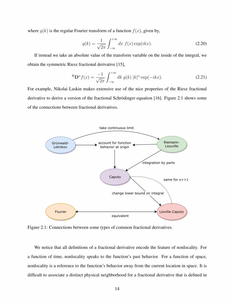
For example, Nikolai Laskin makes extensive use of the nice properties of the Riesz fractional
derivative to derive a version of the fractional Schrodinger equation [16]. Figure 2.1 shows some
of the connections between fractional derivatives.
Figure 2.1: Connections between some types of common fractional derivatives.
We notice that all definitions of a fractional derivative encode the feature of nonlocality. For
a function of time, nonlocality speaks to the function’s past behavior. For a function of space,
nonlocality is a reference to the function’s behavior away from the current location in space. It is
difficult to associate a distinct physical neighborhood for a fractional derivative that is defined in
14
terms of improper integrals. Instead we approach these integrals as an idealized limit that informs
our physical intuition. For example, for a fractional derivative of a function of time, we would not
expect to see an integral that accounts for function behavior over some future time as that would
violate causality. However, we can have a fractional derivative for a function of time that integrates
over the function’s past from some finite point in time. For a function of space, we do not associate
the same directional history and thus we can have fractional derivatives that integrate information
over symmetric intervals. The concept of a finite neighborhood becomes more apparent when
we express fractional derivatives in terms of integer-order derivatives [10]. Each integer-order
derivative accounts for a small portion of the function’s neighborhood such that in summation
the neighborhood overall is nonlocal. Because for some functions we are able to truncate the
integer derivative expansion that stands in place of the fractional derivative, we see that fractional
derivatives are indeed characterized by a finite domain.
In the physical context of fractional derivatives we shall also distinguish between nonlocal
information and memory. While the fractional derivative serves to encode information about the
function’s past, it is stored in aggregate form after the integral or the sum has been computed.
Thus we cannot associate individual events with the present behavior of the function governed by
its fractional derivative. Instead we must consider the aggregate aspect of nonlocality.
2.2 Mathematical background
In Chapter 3 we encounter the fractional Taylor series. The fractional Taylor series serves to
decompose a function f(x) into an infinite sum of fractional derivatives [17],
f(x) =∞∑m=0
(x− a)mα
Γ(mα + 1)(Dα
x)m[f(x)
]|x=a, (2.22)
where it is assumed that the function f(x) is infinitely fractionally-differentiable at a, and that
f(x) is defined to the right of a. Not all fractional derivatives can be used in the fractional Taylor
series. Care must be taken to ensure that the fractional Taylor series holds for any particular type
of fractional derivative.
15
Two functions that we make extensive use of are the Gamma and Mittag-Leffler functions.
We’ve already seen the Gamma function in the Cauchy repeated integration formula, and in the
definitions of the fractional derivative. The Gamma function extends the factorial function from
natural numbers to real numbers. For Re(z) > 0 we have an integral representation of the Gamma
function,
Γ(z) =
∫ ∞0
dt tz−1 exp(−t). (2.23)
Three main properties of the Gamma function are,
Γ(z + 1) = zΓ(z) (2.24)
Γ(z + 1) = z! if z ∈ N (2.25)
Γ(z)Γ(1− z) =π
sin(πz)if z /∈ Z. (2.26)
The Mittag-Leffler function generalizes the series for the exponential, developed by the Swedish
mathematician Gosta Mittag-Leffler in 1903. Characterized by two parameters, α and β, where
Re(α) > 0, the generalized Mittag-Leffler function is given by,
Eα,β(z) =∞∑n=0
zn
Γ(nα + β). (2.27)
We note that when β = 1 the Mittag-Leffler function reduces to a one-parameter Mittag-Leffler
function Eα(z). Similarly, when α = 1 and β = 1, the generalized Mittag-Leffler function E1,1(z)
further reduces to the exponential function exp(z). The Mittag-Leffler function is particularly im-
portant as it is an eigenfunction of the Caputo fractional derivative,Eα[(kz)α
], with the eigenvalue
given by kα [6].
We make an interesting connection for the single-parameter Mittag-Leffler function when it is
of the form Eα(−z2). We note that one special case of the Mittag-Leffler function is E2(−z2) =
cos(z). However, when α = 1 instead, we obtain E1(−z2) = exp(−z2). This tells us about
the distribution of zeros of the single-parameter Mittag-Leffler function when the argument is a
negative quadratic. For the range of values 1 < α < 2, the Mittag-Leffler function Eα(−z2)
goes from having one zero (as z → ∞) to an infinite number of periodic zeros. In other words,
16
when 1 < α < 2, the Mittag-Leffler function Eα(−z2) interpolates between Gaussian and cosine
functions. More information on the properties of the Mittag-Leffler function can be found in [18].
In our study of fractional calculus we also encounter hypergeometric functions (see discus-
sions in Chapters 5 and 6). For completeness we mention some key ideas about hypergeometric
functions.
The generalized hypergeometric function AFB
(~a;~b; z
)is defined in terms of its hypergeomet-
ric series (vector of coefficients ~a has A elements, and vector of coefficients~b has B elements),
AFB
[a1, . . . , aAb1, . . . , bB
; z
]=∞∑n=0
(a1)n · · · (aA)n(b1)n · · · (bB)n
zn
n!, (2.28)
where the Pochhammer symbol (a)n is a ratio of Gamma functions defined by (a)n =Γ(a+ n)
Γ(a).
Gradshteyn and Ryzhik [19] explicitly outline the convergence properties of the hypergeomet-
ric function 2F1 (α, β; γ; z). We have the following three scenarios for the convergence of the
hypergeometric series 2F1 (α, β; γ; z) on the unit circle.
1. The series converges throughout the entire unit circle except at the point z = 1 when
0 ≤ Re(α + β − γ) < 1. (2.29)
2. The series converges absolutely throughout the entire unit circle when
Re(α + β − γ) < 0. (2.30)
3. The series diverges on the entire unit circle when
Re(α + β − γ) ≥ 1. (2.31)
We notice that the conditions for convergence of the hypergeometric series relies on the magni-
tude of the difference between the terms in the numerator and the denominator of the expansion
coefficients for the hypergeometric function.
To understand the convergence properties of the generalized hypergeometric series we apply
the ratio test to the expansion coefficients. We notice that the radius of convergence for the gen-
17
eralized hypergeometric series depends on the number of coefficients in the vector ~a, A, and the
vector ~b, B. If A < B + 1, the ratio of coefficients tends to zero and the hypergeometric series
converges for any finite value of z. If A = B + 1, the ratio of coefficients tends to one and the
series converges for |z| < 1. For |z| > 1 the series diverges. Finally if A > B + 1, the ratio of
coefficients grows without bound and the series diverges except at z = 0.
We note that while we take the convergence of the generalized hypergeometric series for
granted in Chapters 5 and 6, for each elementary function that can be expressed as a generalized
hypergeometric series the convergence properties of the series should be made explicit.
18
CHAPTER 3
FRACTIONAL SCHRODINGER EQUATION IN FRACTIONAL SPACETIME
A paper to be submitted
Gavriil Shchedrin*, Anastasia Gladkina*, and Lincoln D. Carr*
We derive a new form of the fractional Schrodinger equation that explicitly correlates the frac-
tional dimension of the underlying physical geometry with the fractional space derivative replacing
the local kinetic energy term. By assuming two principal postulates used to characterize the proper-
ties of the system’s self-similar topology, namely the fractional spacetime interval that reflects the
mathematical scaling inherent to the system in both space and time coordinates, and the fractional
velocity, the fractional Schrodinger equation captures nonlocal aspects of physical materials with
multiple spatial and temporal scales. By altering the form of the kinetic energy term to include
the fractional space derivative we predict to describe a wide range of physical materials where the
properties of the material are no longer exclusively reliant on the chosen potential, as the kinetic
energy begins to encode the materials’ internal structure. By generalizing the action to include the
Lagrangian in terms of the fractional kinetic energy, we use the time evolution operator and the
fractional Taylor series to expand the Feynman path integral in the leading order. By collecting
leading order terms we come to the exact form of the fractional Schrodinger equation. We per-
form a consistency test and obtain the integer Schrodinger equation in the limit as the fractional
dimension of space and time coordinates tends to integer values. To explore the dynamics of the
fractional Schrodinger equation we solve the infinite potential well problem with different types of
fractional space and time derivatives, and find that the discretized energy scales according to the
fractional space dimension. We find the explicit form of the momentum operator and study parity-
and time-reversal symmetries of the fractional Hamiltonian operator. We see that for the Hamilto-
nian to be parity- and time-reversal-symmetric, the fractional space derivative must be symmetric
*Department of Physics, Colorado School of Mines.
19
and the fractional time derivative must be anti-symmetric. This narrows down which kinds of
fractional derivatives can be considered in the fractional Schrodinger equation.
3.1 Background
The fractional Schrodinger equation has been previously derived by Nikolai Laskin [16], using
the ideas of the Feynman path integral and measures over Levy flights. His analysis assumes
scaled integer-order derivatives, which leads to the use of the quantum Riesz fractional derivative
in the fractional Schrodinger equation. We approach the derivation of the fractional Schrodinger
equation by minimizing the action S, which depends on a scaled spacetime interval. The scaled
spacetime interval is defined in terms of space and time coordinates that are scaled according to
two independent parameters, which determine the self-similar properties of a physical material.
Because the space and time coordinates are scaled in different ways, the velocity in such a medium
can be redefined in terms of a fractional derivative, which we take to be the second basic necessary
postulate to derive the fractional Schrodinger equation. These postulates are self-consistent with
results in relativistic theory and do not require generalizations of already known identities such as
the Einstein relation. Instead, the analysis rests solely on a set of physical principles that naturally
lead to a form of the fractional Schrodinger equation that is applicable to any type of fractional
derivative that follows the fractional Taylor series for the decomposition of a function.
3.2 Action for a particle in fractional spacetime with different fractional dimensions
It is known that self-similar physical geometries endow primary physical variables used to
describe movement within the space with scaling relationships that track its fractional dimension
α. Thus on the basis of assuming that the space we are describing has scaling relationships in
both space and time, characterized by two parameters α and δ respectively, we allow ourselves
to generalize the local spacetime metric and the velocity to reflect the scaling of the underlying
physical geometry. Inherently, of all physical variables present in the description of a quantum
mechanical particle, the kinetic energy is one of the first variables to be affected when considering
movement in a fractional space. Similarly, the spacetime metric must reflect the space and time
20
scalings present in the physical system. We shall note that these assumptions present a unique
perspective in modeling physical materials, as the underlying material is described foremost by
how it affects the kinetic energy and thus the movement of the particle through the system, instead
of allowing the potential energy to formulate prescribed material properties. Without specifying
the potential of the system, we are able to account for spatial and time nonlocality present in the
system by expressing common physical variables in terms of fractional derivatives.
Thus we assume that a point within this physical system will have different scaling orders for
space and time coordinates, α and δ respectively, given by the following scaled spacetime interval,
(dsδ) = (cdtδ, dxα, dyα, dzα). (3.1)
We note that to be consistent with the units of distance in fractional spacetime, the speed of light c
now has units of lengthα/timeδ.
The object central to our analysis is the action S. To account for the fractional spacetime
metric, the action S must be expressed in terms of the scaled spacetime interval dsδ,
S = −a∫dsδ, (3.2)
where a is a proportionality constant. This formulation of the action ensures that the Einstein
relation has no dependence on the scaling of the physical space in terms of α and δ, i.e. it preserves
the original form of the Einstein energy relation.
We briefly show how to derive the form of the Lagrangian L . From Eq. (3.1) the spacetime
interval is given by,
(dsδ)2 = (cdtδ)2 −3∑i=1
(dxαi )2 , (3.3)
where d~x = (dx, dy, dz). Thus we have,
dsδ = cdtδdsδ
cdtδ= cdtδ
[(cdtδ)2 −
∑3i=1(dx
αi )2
(cdtδ)2
]1/2. (3.4)
We assume that the velocity is generalized in terms of two fractional orders, α and δ, to reflect the
underlying physical topology,
21
vi =dxαidtδ
, (3.5)
which simplifies the fractional spacetime interval to,
dsδ = cdtδ
(1−
(v
c
)2)1/2
. (3.6)
Finally, the action S becomes,
S = −a∫dsδ = −ac
∫dtδ
(1−
(v
c
)2)1/2
=
∫dtδ L . (3.7)
By demanding that in the limit v → 0 the Lagrangian of a free particle goes to L = −mc2, we
find a = mc [20]. Then the Lagrangian L of a free particle is given by,
L = −mc2(
1−(v
c
)2)1/2
. (3.8)
With β = v/c, the momentum is given by the first derivative of the Lagrangian with respect to
speed [20],
p =∂L
∂v=
mv√1− β2
. (3.9)
The fractional velocity in Eq. (3.5) in terms of the two fractional orders α and δ allows the particle
to move faster or slower than in standard Euclidean space as fractional space encodes within itself
a nonlocality that changes the dynamics of the system. The units of fractional velocity, similar to
the units for the speed of light c in a self-similar medium, scale as lengthα/timeδ.
3.3 Derivation of the Schrodinger equation via a Feynman path integral
First of all we shall introduce the fractional Taylor series [17],
f(x) =∞∑m=0
(x− x0)mδ
Γ(mδ + 1)
(Dδx
)m[f(x)]
∣∣∣∣x=x0
, (3.10)
which we will use to expand the time evolution operator.
The time evolution operator is given by [21],
22
ψ(xα, (t+ ε)δ
)=
1
A
∫ ∞−∞
dyα exp
(i
hS
)ψ(yα, tδ
), (3.11)
where A is a normalization constant and we take ε to be a small increment in time defined by
ε = ∆t. Here the action S from Eq. (3.2) is,
S =
∫ t+ε
t
dtδ L
(x,dxα
dtδ, t
). (3.12)
Following Feynman we choose a quadratic Lagrangian,
L = T − U =m
2
(dxα
dtδ
)2
− V(xα, tδ
). (3.13)
The left-hand side follows from the fractional Taylor expansion,
ψ(xα, (t+ ε)δ
)= ψ
(xα, tδ
)+
εδ
Γ (δ + 1)
(Dδt
) [ψ(xα, tδ)
]+ O
(ε2δ). (3.14)
The task is to collect all the terms from the right-hand side of the order εδ.
The discretization scheme is as follows:
xα =
(xn+1 + xn
2
)α≡(x+ y
2
)α, (3.15)
v =dxα
dtδ≡ (xn+1 − xn)α
(tn+1 − tn)δ=
(x− y)α
εδ.
Here we denoted,
xn+1 = x, (3.16)
xn = y, (3.17)
tn+1 − tn = ε. (3.18)
We notice that other discretization schemes, such as xα =(xαn+1 + xαn
)/2, lead to alternative
forms of the fractional kinetic energy with a nonlinear dependence on α. The chosen discretization
scheme avoids introducing any unphysical dependence of the kinetic energy on α or δ.
23
The action S then becomes,
S =
∫ t+ε
t
dtδ L
(x,dxα
dtδ, t
)=
∫ t+ε
t
dtδ
[m
2
(dxα
dtδ
)2
− V(xα, tδ
)](3.19)
=
m2
(|x− y|α
εδ
)2
− V
((x+ y
2
)α, tδ
) εδ.Let’s introduce,
y = x+ η, (3.20)
η = yn+1 − yn. (3.21)
Then we have,
ψ(xα, (t+ ε)δ
)= (3.22)
=1
A
∫ ∞−∞
dyα exp
[iεδ
h
m
2
(|x− y|α
εδ
)2]
exp
−iεδhV
((x+ y
2
)α, tδ
)ψ (yα, tδ) =
1
A
∫ ∞−∞
dηα exp
[iεδ
h
m
2
∣∣∣∣ηαεδ∣∣∣∣2]
exp
−iεδhV
((2x+ η
2
)α, tδ
)ψ ((x+ η)α, tδ). (3.23)
Here we have approximated,
dyα = limη→0
∆(yn+1 − yn)α = limη→0
∆ηα = dηα. (3.24)
We note that the Gaussian-like function,
exp
[iεδ
h
m
2
∣∣∣∣ηαεδ∣∣∣∣2], (3.25)
exponentially oscillates away from η = 0.
24
We will expand the wave function up to second order in η,
ψ(yα, tδ) =∞∑m=0
(y − x)mα
Γ (mα + 1)(Dα
x)m [ψ(x, t)] (3.26)
= ψ(xα, tδ) +ηα
Γ (α + 1)(Dα
x)[ψ(xα, tδ)
]+
η2α
Γ (2α + 1)(Dα
x)2[ψ(xα, tδ)
]+ O
(η3α).
The next step is to expand the potential,
exp
−iεδhV
((2x+ η
2
)α, tδ
) = 1− iεδ
hV
((2x+ η
2
)α, tδ
)+ O
(ε2δ). (3.27)
We collect all the terms,
ψ(xα, (t+ ε)δ
)= (3.28)
=1
A
∫ ∞−∞
dηα exp
[iεδ
h
m
2
∣∣∣∣ηαεδ∣∣∣∣2]
exp
−iεδhV
((2x+ η
2
)α, tδ
)ψ ((x+ η)α, tδ)
=1
A
∫ ∞−∞
dηα exp
[iεδ
h
m
2
∣∣∣∣ηαεδ∣∣∣∣2]×
1− iεδ
hV
((2x+ η
2
)α, tδ
)+ O
(ε2δ) (3.29)
×
(ψ(xα, tδ) +
ηα
Γ (α + 1)(Dα
x)[ψ(xα, tδ)
]+
η2α
Γ (2α + 1)(Dα
x)2[ψ(xα, tδ)
]).
On the other hand, we have,
ψ(xα, (t+ ε)δ
)= ψ
(xα, tδ
)+
εδ
Γ (δ + 1)
(Dδt
) [ψ(xα, tδ)
]+ O
(ε2δ). (3.30)
Thus we demand from the leading term,
1 =1
A
∫ ∞−∞
dηα exp
[iεδ
h
m
2
∣∣∣∣ηαεδ∣∣∣∣2]. (3.31)
We introduce,
25
ξ = ηα, (3.32)
dξ = dηα,
a =m
2hεδ.
Therefore, we get,
1 =1
A
∫ ∞−∞
dξ exp
[im
2h
ξ2
εδ
]. (3.33)
We are dealing with the complex Gaussian integral,
I =
∫ ∞−∞
dξ exp[iaξ2
]=
√iπ
aexp[iπα]. (3.34)
Therefore, we obtain,
A = I =
∫ ∞−∞
dηα exp
[iεδ
h
m
2
∣∣∣∣ηαεδ∣∣∣∣2]
=
∫ ∞−∞
dξ exp
[im
2h
ξ2
εδ
]=
√2iπhεδ
m. (3.35)
We shall collect all the terms of the order εδ.
The first one is,
1
A
∫ ∞−∞
dηα exp
[iεδ
h
m
2
∣∣∣∣ηαεδ∣∣∣∣2]×
−iεδhV
((2x+ η
2
)α, tδ
)ψ(xα, tδ) (3.36)
=1
A
[−iε
δ
hV(xα, tδ
)ψ(xα, tδ)
]∫ ∞−∞
dηα exp
[iεδ
h
m
2
∣∣∣∣ηαεδ∣∣∣∣2]
+ O(ε2δ)
= −iεδ
hV(xα, tδ
)ψ(xα, tδ). (3.37)
The next term is zero due to the integral of an odd function integrated over a symmetric interval,
1
A
∫ ∞−∞
dηα exp
[iεδ
h
m
2
∣∣∣∣ηαεδ∣∣∣∣2]×(
ηα
Γ (α + 1)(Dα
x)[ψ(xα, tδ)
])(3.38)
=1
A
∫ ∞−∞
dξ exp
[−aξ
2
i
](ξ
Γ (α + 1)(Dα
x)[ψ(xα, tδ)
])= 0.
26
The final piece is,
1
A
∫ ∞−∞
dηα exp
[iεδ
h
m
2
∣∣∣∣ηαεδ∣∣∣∣2]×
(η2α
Γ (2α + 1)(Dα
x)2[ψ(xα, tδ)
])(3.39)
=1
A
∫ ∞−∞
dξ exp
[−aξ
2
i
](ξ2
Γ (2α + 1)(Dα
x)2[ψ(xα, tδ)
]).
The Gaussian integral,
∫ ∞−∞
dξ exp
[−aξ
2
i
]ξ2 = −i ∂
∂a
∫ ∞−∞
dξ exp
[−aξ
2
i
]= −i ∂
∂a
√iπ
a=
i
2a
√iπ
a. (3.40)
Therefore we get,
1
A
∫ ∞−∞
dξ exp
[−aξ
2
i
](ξ2
Γ (2α + 1)(Dα
x)2[ψ(xα, tδ)
])(3.41)
=1
A
(1
Γ (2α + 1)(Dα
x)2[ψ(xα, tδ)
])∫ ∞−∞
dξ exp
[−aξ
2
i
]ξ2
=1
A
(1
Γ (2α + 1)(Dα
x)2[ψ(xα, tδ)
]) i
2
2hεδ
m.
We shall collect all the terms,
ψ(xα, (t+ ε)δ) = ψ(xα, tδ) +εδ
Γ (δ + 1)
(Dδt
) [ψ(xα, tδ)
](3.42)
= ψ(xα, tδ)− iεδ
hV(xα, tδ
)ψ(xα, tδ) +
(1
Γ (2α + 1)(Dα
x)2[ψ(xα, tδ)
]) i
2
2hεδ
m.
In other words, we have,
εδ
Γ (δ + 1)
(Dδt
) [ψ(xα, tδ)
]= (3.43)
= −iεδ
hV(xα, tδ
)ψ(xα, tδ) +
(1
Γ (2α + 1)(Dα
x)2[ψ(xα, tδ)
]) ihεδ
m. (3.44)
If we multiply both parts by ih, we arrive at the fractional Schrodinger equation,
27
ih
Γ (δ + 1)
(Dδt
) [ψ(xα, tδ)
]=
−h2
Γ (2α + 1)m(Dα
x)2[ψ(xα, tδ)
]+ V
(xα, tδ
)ψ(xα, tδ). (3.45)
3.4 Limit to obtain the integer Schrodinger equation
We note that all fractional derivatives must limit to integer-order derivatives (up to a constant)
when the order of the derivative is chosen to be an integer [6]. Thus in the special case of,
δ = 1, (3.46)α = 1,
we recover the integer Schrodinger equation,
ih∂ψ(x, t)
∂t=−h2
2m
∂2ψ(x, t)
∂x2+ V (x, t)ψ(x, t). (3.47)
3.5 Solution to the infinite potential well
As a test problem let’s consider a fractional Schrodinger equation with a Caputo time derivative
of order δ and a Fourier space derivative of order 2α for 0 < α < 1,
ih
Γ(δ + 1)
(CDδ
t
) [ψ(xα, tδ)
]=
−h2
Γ(2α + 1)m
(FD
2α
x
) [ψ(xα, tδ)
]+ V
(xα, tδ
)ψ(xα, tδ). (3.48)
We employ separation of variables ψ(x, t) = f(x)g(t) to obtain two equations,
ih
Γ(δ + 1)CD
δ
t
[g(t)
]= Eg(t), (3.49)
−h2
Γ(2α + 1)mFD
2α
x
[f(x)
]+ V (x)f(x) = Ef(x), (3.50)
where we assumed the potential V = V (x) is only a function of spatial coordinates, and E is
our energy eigenvalue. The solution to Eq. (3.49) can be expressed in terms of a single-parameter
Mittag-Leffler function, Eδ(λtδ) (see Eq. (2.27) in Chapter 2 for its definition),
28
g(t) =∞∑k=0
(E Γ(δ + 1)
ih
)ka0
Γ(kδ + 1)tkδ = a0
∞∑k=0
(λ tδ)k
Γ(kδ + 1)≡ a0Eδ(λt
δ), (3.51)
where a0 is a value related to the normalization of our wavefunction, namely that ψ(x, 0) =
f(x)g(0) = a0f(x), and λ =(−iE Γ(δ + 1)
)/h. The wide tilde on Eδ(λtδ) differentiates be-
tween the Mittag-Leffler function and the energy eigenvalue found inside λ.
We use the ansatz f(x) = exp(kx) to find the solution to Eq. (3.50). For constant V (x) = V0,
we then obtain a polynomial equation in the momentum variable k,
−h2
Γ(2α + 1)mk2α + V0 = E, (3.52)
k± = exp
(± iπ
2α
)(1
h
) 1α [
(E − V0) Γ(2α + 1)m] 1
2α . (3.53)
Quantization of k and E come from boundary conditions (which come from the type of potential
we use). Consider an infinite potential well given by,
V (x) =
∞ if x ≤ 0
0 if 0 < x < L
∞ if x ≥ L
(3.54)
on the domain 0 ≤ x ≤ L. Then we require that the spatial component of the wavefunction decays
at the boundaries, f(x)|x=0 = f(x)|x=L = 0. From Eq. (3.53) we obtain two roots, k±, for when
V (x) = 0. By enforcing the boundary conditions we quantize k±,
k± = exp
(±iπ
2α
)1
sin(π2α
) nπL, where n ∈ Z+. (3.55)
We can simplify the spatial component of the wavefunction from f(x) = A exp(k+x)+B exp(k−x),
with A and B new undetermined coefficients, to
f(x) = A exp
[cot
(π
2α
)nπx
L
]sin
(nπx
L
). (3.56)
Finally we obtain the following dispersion relation,
29
En =h2(nπL
csc(π2α
))2αΓ(2α + 1)m
. (3.57)
We note that when α = 1, we find the expected energy spectrum for an infinite potential well,
En =
(nπh
L
)21
2m. (3.58)
In comparison, the fractional Schrodinger equation developed by Nikolai Laskin has the following
discretized energy spectrum for an infinite potential well [22],
En = D2α
(nπh
L
)2α
, (3.59)
where D2α is a physical constant that accounts for mass. We note that h is scaled according to the
fractional space dimension α.
The solution to the fractional Schrodinger equation with a Caputo time derivative of order δ
and a Fourier space derivative of order 2α in a given infinite potential well is expressed as,
ψ(x, t) = f(x)g(t) = A exp
[cot
(π
2α
)nπx
L
]sin
(nπx
L
)Eδ(λt
δ), (3.60)
where λ =(−iE Γ(δ + 1)
)/h, and a0 has been absorbed into A for ease of notation.
3.6 The form of the fractional Hamiltonian and momentum operators
From Eqs. (3.9) and (3.5) we have the relativistic definition of momentum in terms of fractional
velocity,
p =mv√1− β2
=m√
1− β2
dxα
dtδ. (3.61)
The fractional Schrodinger equation gives us an alternate definition of momentum from the kinetic
energy term. We find that while physical variables change definitions, the principal mathematical
form of the kinetic energy stays the same. This is similar to how the momentum operator is
redefined in fractional spacetime in terms of fractional velocity, while retaining its form in terms
of mass and the Lorentz factor. From Eq. (3.45) we find that the kinetic energy T is expressed by
30
the square of the fractional momentum operator p,
T =−h2
Γ(2α + 1)m
∂2α
∂x2α=
p2
Γ(2α + 1)m, (3.62)
p ≡ −ih ∂α
∂xα. (3.63)
Then in d = 1 dimension our Hamiltonian H appears as,
H =p2
Γ(2α + 1)m+ V (x, t). (3.64)
By comparison, the Hamiltonian developed by Nikolai Laskin [16] features an integer derivative
momentum operator scaled to a fractional power,
H = Dα |p|α + V (x, t), (3.65)
p = −ih ∂∂x, (3.66)
where Dα represents a physical constant that accounts for mass. Because the entire momentum
operator is scaled, h is also scaled adjusting its natural units to fractional units. Similarly to avoid
problems with scaling the imaginary unit i, the magnitude of the momentum operator is considered.
The ad hoc scaling of the entire momentum operator changes the form of the kinetic energy such
that it no longer follows the square of the velocity, raising the question of how to account for mass
and any additional constant factors out front.
The Hamiltonian developed in this paper avoids problems associated with scaling any physical
system parameters. We think of h as the granularity of physical space that cannot be broken
down into any smaller pieces, like an atom. But if kinetic energy is expressed in terms of hα,
what stops us from redefining a new integral h that is in terms of the root of the old h? This
ambiguity is avoided if physical variables relating to how we view physical space are expressed in
terms of fractional derivatives, and the overall form of the Hamiltonian and momentum operators
is preserved.
31
3.7 Symmetry properties of the fractional Schrodinger equation
We consider different types of symmetries to better characterize the fractional Schrodinger
equation. Spatial inversion is an important type of symmetry that holds for the regular Schrodinger
equation when the potential is also space-symmetric (even symmetry). However, in the fractional
Schrodinger equation spatial symmetry largely depends on the type of fractional derivative chosen.
Some derivatives, like the Riesz derivative, are explicitly space-symmetric, while others are not.
In the position basis, to check for PT symmetry we perform the following rotations,
Parity reversal : x→ −x,Time reversal : i→ −i, t→ −t.
(3.67)
However, this assumes that t→ −t and i→ −i are reciprocal operations (since the time derivative
in the regular Schrodinger equation is multiplied by ih). In general this will not be true for a frac-
tional time derivative in the fractional Schrodinger equation, and we have to make the symmetries
of space and time fractional derivatives more explicit. We would expect to collect a minus sign on
the time derivative from taking t → −t while all other terms are invariant, if the Hamiltonian is
indeed PT-symmetric. With these rotations we obtain,
−ihΓ(δ + 1)
(Dδ−t
)ψ∗(χα, τ δ) =
−h2
Γ(2α + 1)m
(Dα−x
)2ψ∗(χα, τ δ) + V
(χα, τ δ
)ψ∗(χα, τ δ), (3.68)
where χ and τ replace the transformed variables in the wavefunction, and ψ∗(χ, τ) denotes wave-
function conjugation that comes from taking i → −i. Here we use χ = −x and τ = −t. For PT
symmetry to be satisfied we see that we would want to have a time derivative that is anti-symmetric
(as is true for all odd derivatives) so that Dδ−t = −Dδ
t . Similarly we would want the Hamiltonian to
be invariant under an x → −x transformation, which forces both the space derivative and the po-
tential to be symmetric such that(Dα−x
)2=(Dαx
)2≡(D2αx
)and V (−x,−t) = V (x, t). If the
space and time derivatives satisfy these requirements, and the potential is even, then the fractional
Schrodinger equation is invariant under parity and time reversal and the transformed wavefunction
ψ∗(χ, τ) must evolve according to the same dynamics as ψ(x, t). We are free to choose the po-
32
tential we want; however, the space derivative in general has direction bias and space is no longer
homogeneous, meaning that∂α
∂(−x)α6= − ∂α
∂xα. This is the difference between left-handed and
right-handed derivatives.
Consider, for example, the left-sided Riemann-Liouville derivative, given by,
RLDαaf(x) =
1
Γ(n− α)
dn
dxn
∫ x
a
dt (x− t)n−α−1f(t). (3.69)
The derivative is with respect to the argument of the function, therefore, to find ∂α
∂(−x)α we take
a derivative of a function with negative argument, f(−x). Because we change variables x → t
inside the integral, t now becomes −t. Similarly, x denotes the upper bound and because we take
x → −x, the integer derivatives are now with respect to −x, and we take x → −x inside the
integral. With these transformations we obtain,
RLDαaf(−x) =
−1
Γ(n− α)
dn
d(−x)n
∫ −xa
dt (t− x)n−α−1f(−t), (3.70)
RLDαaf(−x) =
(−1)n
Γ(n− α)
dn
dxn
∫ a
x
dt (t− x)n−α−1f(−t), (3.71)
where in the last step we change the bounds of the integral because by definition a ≤ x. We notice
this is indeed the right-sided Riemann-Liouville fractional derivative. Indeed the directional bias
of the derivative reverses under parity reversal.
The disparity in symmetry between space and time fractional derivatives comes from causality.
It is possible for a system to be spatially nonlocal and thus at one point contain information about
a large symmetric neighborhood around it. However, with the time axis we can no longer sample
the future neighborhood. A fractional time derivative then is characterized by an arrow that differ-
entiates the past from the future. As time steps forward, we accumulate memory that accounts for
past function behavior.
We see that fractional derivatives offer us a direction bias that breaks PT symmetry. PT-
symmetric Hamiltonians can be built by carefully selecting the time and space derivatives such
that the spatial dimensions are symmetric and the time dimension is anti-symmetric. If the frac-
tional Schrodinger equation is not PT-invariant, the energy spectrum will have complex eigenvalues
33
and the system will have a gain/loss mechanism in terms of energy and norm.
Similarly the potential energy needs to have even space symmetry and odd time symmetry for
the Hamiltonian to be PT-symmetric. While the internal structure of the material informs the frac-
tional derivative form of the kinetic energy, we can introduce an external potential that results in an
easily controllable physical system. In particular, we hypothesize that a wide range of multiscale
potentials can reproduce the behavior of the fractional Schrodinger equation by endowing the po-
tential energy with the nonlocal properties we initially sought in the kinetic energy. After all, as
long as total energy stays the same, we can exchange kinetic for potential energy and vice versa.
34
CHAPTER 4
EXPANSION OF FRACTIONAL DERIVATIVES IN TERMS OF AN INTEGER DERIVATIVE
SERIES: PHYSICAL AND NUMERICAL APPLICATIONS
A paper submitted to the Journal of Mathematical Physics, arXiv:1710.06297† (2017) [10]
Anastasia Gladkina‡, Gavriil Shchedrin‡, U. Al Khawaja*, and Lincoln D. Carr‡
We use the displacement operator to derive an infinite series of integer order derivatives for the
Grunwald-Letnikov fractional derivative and show its correspondence to the Riemann-Liouville
and Caputo fractional derivatives. We demonstrate that all three definitions of a fractional deriva-
tive lead to the same infinite series of integer order derivatives. We find that functions normally rep-
resented by Taylor series with a finite radius of convergence have a corresponding integer derivative
expansion with an infinite radius of convergence. Specifically, we demonstrate robust convergence
of the integer derivative series for the hyperbolic secant (tangent) function, characterized by a finite
radius of convergence of the Taylor series R = π/2, which describes bright (dark) soliton propa-
gation in nonlinear media. We also show that for a plane wave, which has a Taylor series with an
infinite radius of convergence, as the number of terms in the integer derivative expansion increases,
the truncation error decreases. Finally, we illustrate the utility of the truncated integer derivative
series by solving two linear fractional differential equations, where the fractional derivative is re-
placed by an integer derivative series up to the second order derivative. We find that our numerical
results closely approximate the exact solutions given by the Mittag-Leffler and Fox-Wright func-
tions. Thus, we demonstrate that the truncated expansion is a powerful method for solving linear
fractional differential equations, such as the fractional Schrodinger equation.
†Permission is provided by the Non-exclusive license to distribute used for this ArXiv submission.‡Department of Physics, Colorado School of Mines.*Department of Physics, United Arab Emirates University.
35
4.1 Introduction
Fractional calculus is a powerful tool to describe physical systems characterized by multiple
time and length scales, nonlocality, fractional geometry, non-Gaussian statistics, and non-Fickian
transport [14, 23]. Anomalous diffusion through disordered media [5, 24], hydrogeologic treatment
of water propagation through soil and rocks [8, 25, 26], Levy flights [27], and turbulence [28]
are among the physical phenomena that can be consistently described within the framework of
fractional calculus [6, 7, 29]. Similarly, certain biological systems, e.g., neuron clusters and heart
cell arrays, exhibit multiple time scales that define fractional dynamics of the biological response
to external stimuli [30, 31].
The building block of fractional calculus is a fractional derivative. There are multiple ways to
generalize an integer order derivative to fractional order, and in this paper we exclusively concen-
trate on the Riemann-Liouville, Caputo, and Grunwald-Letnikov definitions [23]. The Riemann-
Liouville and Caputo definitions are integral forms of the fractional derivative, especially suit-
able for solving linear fractional differential equations (FDEs) [14, 23]. The Grunwald-Letnikov
derivative is a discrete form of the fractional derivative, represented by a function summed over its
history, and is primarily used in numerical methods to solve linear FDEs. The Grunwald-Letnikov
derivative gives a computationally straightforward way to find the fractional derivative of an arbi-
trary function, yet it provides no direction towards finding its explicit analytical form. Except for
a few trivial cases, where a fractional derivative can be expressed in terms of elementary or special
functions, the Riemann-Liouville and Caputo derivatives also lead to expressions that are implicit
or indirect [6, 14, 23].
Despite the fact that Riemann-Liouville, Caputo, and Grunwald-Letnikov definitions are three
different forms of the fractional derivative, there is a correspondence between them. Although
the Grunwald-Letnikov derivative is a discrete fractional derivative and the Riemann-Liouville
derivative is continuous, it was shown that both definitions are equivalent in the continuous limit
[14, 23]. The Caputo fractional derivative can be obtained from the Riemann-Liouville fractional
derivative by accounting for the initial conditions of a function at the expansion point. The ac-
36
count of the initial conditions in the Caputo definition leads to a convergent form of the fractional
derivative at the expansion point, in contrast to both Grunwald-Letnikov and Riemann-Liouville
derivatives, which makes it especially suitable for physical applications [6]. In this article, we
derive the exact analytical formula that casts the Grunwald-Letnikov fractional derivative into an
infinite sum of integer order derivatives. By representing the fractional derivative as an infinite
series of integer order derivatives, we find a unified description of Riemann-Liouville, Caputo, and
Grunwald-Letnikov fractional derivatives. The only difference in our expansion for the Riemann-
Liouville or Grunwald-Letnikov derivative and the Caputo derivative is in the lower limit of the
summation index.
We examine convergence of the Grunwald-Letnikov fractional derivative, represented by an
infinite series of integer derivatives, by truncating the infinite series and retaining only the first few
terms. We find that functions normally characterized by Taylor series with a finite radius of con-
vergence have an infinite radius of convergence in the integer derivative expansion. For physically
relevant functions, such as hyperbolic tangent and secant, we show that by retaining only the first
few terms in the infinite series the proposed formula efficiently approximates the fractional deriva-
tive, establishing a firm ground for its use in numerically solving fractional differential equations.
Moreover, we show that for functions represented by Taylor series with an infinite radius of conver-
gence, the truncation error is inversely proportional to the number of terms kept in the expansion.
Specifically, an integer derivative expansion of sin(x) with 2 terms achieves an average 1% error,
and with a total of 10 terms, the error decreases down to 0.01%.
Finally, we use the truncated integer derivative series to solve linear fractional differential
equations with both constant and variable coefficients. We find that the fourth-order Runge-Kutta
method applied to truncated fractional differential equations produces numerical solutions which
rapidly converge to the exact analytical results, given by the Mittag-Leffler and generalized Fox-
Wright special functions [23]. Approximating the fractional derivative as an integer derivative
series with the first 3 terms generates around 1% error for the constant coefficient differential equa-
tion, and 10% error for the differential equation with variable coefficients. Thus, we show that the
37
truncated expansion provides a robust numerical scheme for solving linear fractional differential
equations, such as the fractional Schrodinger and fractional diffusion equations [6].
4.2 Expressing Grunwald-Letnikov fractional derivative as integer derivative series
In this Section we derive the infinite integer derivative expansion for the Grunwald-Letnikov
fractional derivative. For simplicity we only consider left-sided derivatives of order q, with q ∈ C,
subject to constraint of Re(q) > 0.
We adopt the following definition of the Grunwald-Letnikov derivative [23]:
GLDqf(x) = limh→0N→∞
1
hq
N−1∑j=0
(−1)j(q
j
)f(x− jh), (4.1)
where N is the number of gridpoints and h is the grid spacing defined as h ≡ x/N . The infinitesi-
mal step h is a constant until we perform the continuous limit. The generalized binomial coefficient(qj
)valid for non-integer q is defined as [14, 23],
(q
j
)≡ Γ(q + 1)
Γ(j + 1) Γ(q − j + 1)=
(−1)j−1 q Γ(j − q)Γ(1− q) Γ(j + 1)
, (4.2)
where Γ(z) is the Euler gamma function. We note that the function f(x −mh) can be expressed
in terms of the function f(x) via the finite displacement, or shift, operator [21],
f(x− jh) = Djh
[f(x)
]=
(1− h d
dx
)jf(x), (4.3)
which can be verified directly via, e.g., the finite difference method. If we make the substitution,
the Grunwald-Letnikov derivative becomes,
GLDqf(x) = limh→0N→∞
1
hq
N−1∑j=0
(−1)j(q
j
)(1− h d
dx
)jf(x) (4.4)
= limh→0N→∞
N−1∑k=0
N−1∑j=k
hk−q (−1)j−k(q
j
) (j
k
)dk
dxkf(x), (4.5)
38
where we applied the Newton binomial formula to the displacement operator and exchanged the
order of the summation. Now we notice that we can perform the summation of the inner series,
N−1∑j=k
(−1)j−k
j
k
q
j
=(−1)N−k+1(N − k)
q − k
N
k
q
N
. (4.6)
We point out that below we treat the integer case of q ∈ N separately (see Eq. (4.15)). Thus, we
cast the Grunwald-Letnikov derivative into an infinite sum of integer order derivatives,
GLDqf(x) = limh→0N→∞
N−1∑k=0
(−1)N−k+1 (N − k) hk−q
q − k
(N
k
) (q
N
)dk
dxkf(x). (4.7)
To perform the limits h→ 0 andN →∞, we explore the weight function of the integer derivative,
which we define as,
W (q, k,N) =(−1)N−k+1 (N − k) hk−q
q − k
(N
k
)(q
N
), (4.8)
and expand it for N � 1 in a series in 1/N . We obtain,
W (q, k,N) = (4.9)
(−1)N−k(
1
N
)q−k hk−q sin[π(N − q)
]Γ(q + 1)
πΓ(k + 1)
(1
k − q− k + q + 1
2N+ O
(1
N
)2). (4.10)
The leading term in this expansion can be simplified to,
limh→0N→∞
W (q, k,N) = limh→0N→∞
sin[π(q − k)
]Γ(q + 1)
π (q − k) Γ(k + 1)(hN)k−q (4.11)
=sin[π(q − k)
]π (q − k)
Γ(q + 1)
Γ(k + 1)xk−q. (4.12)
Thus, we have performed the expansion of the Grunwald-Letnikov fractional derivative in terms
of integer order derivatives in the limiting case of infinitesimally small grid size h→ 0. Lastly, we
obtain our final series,
39
GLDqf(x) =∞∑k=0
sin[π(q − k)
]π (q − k)
Γ(q + 1)
Γ(k + 1)xk−q
dk
dxkf(x) (4.13)
=∞∑k=0
(q
k
)xk−q
Γ(k − q + 1)
dk
dxkf(x). (4.14)
We note that for integer q ∈ N, the expansion reduces to a single term due to the delta-function
behavior of sinc[π(q − k)]. Indeed for integer q = n we have,
sin[π(q − k)
]π (q − k)
∣∣∣∣∣q=n∈N
= δn,k. (4.15)
Thus the infinite series of integer order derivatives reduces to a single derivative of the nth order,
GLDqf(x)∣∣∣q=n∈N
=dn
dxnf(x). (4.16)
4.3 Unified description of fractional derivatives in terms of the infinite series of integerorder derivatives
In this Section we establish a connection between Riemann-Liouville, Caputo, and Grunwald-
Letnikov derivatives. The Riemann-Liouville fractional derivative is defined as a convolution inte-
gral,
RLDqf(x) =1
Γ(n− q)dn
dxn
∫ x
a
dt (x− t)n−q−1f(t), (4.17)
where n is the ceiling of the fractional order, n = dqe, given in terms of the integer part [q] of q as
dqe = [q] + 1. By rewriting the fractional Riemann-Liouville derivative of order q as a sequential
operation of an integer derivative of order [q] + 1 and a fractional Riemann-Liouville derivative
of order q − dqe, with a subsequent term-by-term fractional differentiation, one obtains an integer
derivative expansion for the Riemann-Liouville fractional derivative [14],
RLDqf(x) =∞∑k=0
(q
k
)(x− a)k−q
Γ(k − q + 1)f (k)(x), (4.18)
40
where a is the base point of the Riemann-Liouville derivative. By choosing a zero base point a = 0
and comparing our formula Eq. (4.13) for the Grunwald-Letnikov derivative with the expansion
derived for the Riemann-Liouville derivative Eq. (4.18), we conclude that the Grunwald-Letnikov
fractional derivative given by Eq. (4.1) and the Riemann-Liouville fractional derivative given by
Eq. (4.17) are not only equivalent in the continuous limit but also lead to the very same infinite
expansion of integer order derivatives.
In order to obtain a unified description for all three fractional derivatives, we introduce the
Caputo fractional derivative, defined according to [23],
CDqf(x) =1
Γ(n− q)
∫ x
a
dt (x− t)n−q−1dnf(t)
dtn. (4.19)
First, we refer to the connection between Caputo and Riemann-Liouville fractional derivatives in
[23],
CDqf(x) = RLDq
f(x)−n−1∑k=0
f (k)(a)
k!(x− a)k
, (4.20)
where integer order derivatives are evaluated at the base point a, i.e.
f (k)(a) ≡ dkf(x)
dxk
∣∣∣∣∣x=a
. (4.21)
By applying the infinite expansion in Eq. (4.13), we obtain,
CDqf(x) ≡ limN→∞
CDq
Nf(x) (4.22)
= limN→∞
N∑j=0
(q
j
)(x− a)j−q
Γ(j − q + 1)
f (j)(x)−n−1∑k=j
f (k)(a)
(k − j)!(x− a)k−j
. (4.23)
We see that Eq. (4.13) is versatile because it bundles all three fractional derivatives into a single
expansion, with a simple adjustment on the lower bound for the Caputo derivative series and a zero
base point on the Riemann-Liouville and Caputo fractional derivatives. Thus, the integer derivative
expansion in Eqs. (4.13), (4.18), and Eq. (4.22) gives a universal formulation for all three fractional
41
derivatives. This universality is an important consistency test for fractional calculus. Moreover, the
infinite expansion in Eq. (4.13) is particularly convenient for numerical implementation in linear
FDEs, as we present in the following Sections.
4.4 Truncation, error, and radius of convergence
In the previous Section we obtained the unified description of Grunwald-Letnikov, Riemann-
Liouville, and Caputo fractional derivatives in terms of an infinite series of integer order deriva-
tives. Even though the infinite expansion of the Riemann-Liouville fractional derivative was de-
rived previously [14], the numerical applications of the result in Eq. (4.13) and Eq. (4.17), which
necessarily rely on the truncation of the infinite series, were missing. The goal of this Section
is to truncate the infinite series given by Eq. (4.13) and calculate the residual truncation error for
several physically relevant functions. To determine the error introduced by truncating the series,
we perform multiple case studies in which we consider functions with both an infinite radius of
convergence of the Taylor series, such as plane and standing waves, Gaussian function, as well as
functions with a finite radius of convergence, e.g., hyperbolic secant (hyperbolic tangent) which
describe bright (dark) soliton propagation. Moreover, we evaluate the minimal number of terms
kept in the infinite series which correspond to a given level of accuracy. In particular, we choose
the Caputo fractional derivative of the order q = 1/2. We calculate relative error by,
ε(x) =a(x)− b(x)
12(|a(x)|+ |b(x)|)
, (4.24)
where a(x) = CDqf(x) is the infinite series given by Eq. (4.22) and b(x) = CDqNf(x) is the
truncated series, where q is the order of the fractional differential operator, and N is the number of
terms in the truncated series Eq. (4.22). We observe spikes in the log-error, log(|ε(x)|), either in
case of real-valued roots of the fractional derivative a(x) or its approximation b(x), or in the case
of a match between the fractional derivative and its approximation. Yet another discontinuity in the
error arises if the fractional derivative and its approximation are of equal magnitude but opposite
in sign.
42
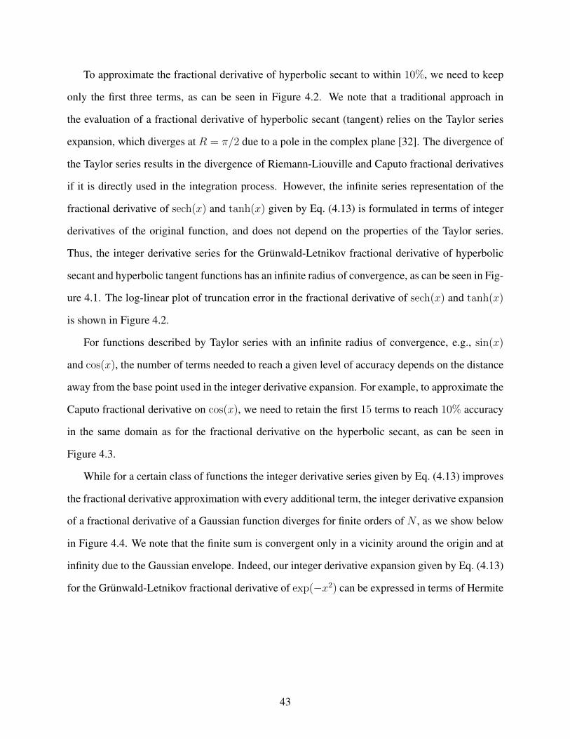
To approximate the fractional derivative of hyperbolic secant to within 10%, we need to keep
only the first three terms, as can be seen in Figure 4.2. We note that a traditional approach in
the evaluation of a fractional derivative of hyperbolic secant (tangent) relies on the Taylor series
expansion, which diverges at R = π/2 due to a pole in the complex plane [32]. The divergence of
the Taylor series results in the divergence of Riemann-Liouville and Caputo fractional derivatives
if it is directly used in the integration process. However, the infinite series representation of the
fractional derivative of sech(x) and tanh(x) given by Eq. (4.13) is formulated in terms of integer
derivatives of the original function, and does not depend on the properties of the Taylor series.
Thus, the integer derivative series for the Grunwald-Letnikov fractional derivative of hyperbolic
secant and hyperbolic tangent functions has an infinite radius of convergence, as can be seen in Fig-
ure 4.1. The log-linear plot of truncation error in the fractional derivative of sech(x) and tanh(x)
is shown in Figure 4.2.
For functions described by Taylor series with an infinite radius of convergence, e.g., sin(x)
and cos(x), the number of terms needed to reach a given level of accuracy depends on the distance
away from the base point used in the integer derivative expansion. For example, to approximate the
Caputo fractional derivative on cos(x), we need to retain the first 15 terms to reach 10% accuracy
in the same domain as for the fractional derivative on the hyperbolic secant, as can be seen in
Figure 4.3.
While for a certain class of functions the integer derivative series given by Eq. (4.13) improves
the fractional derivative approximation with every additional term, the integer derivative expansion
of a fractional derivative of a Gaussian function diverges for finite orders of N , as we show below
in Figure 4.4. We note that the finite sum is convergent only in a vicinity around the origin and at
infinity due to the Gaussian envelope. Indeed, our integer derivative expansion given by Eq. (4.13)
for the Grunwald-Letnikov fractional derivative of exp(−x2) can be expressed in terms of Hermite
43
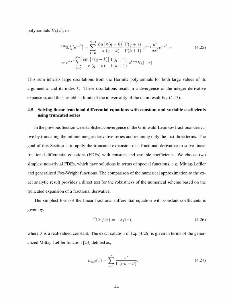
polynomials Hk(x), i.e.
GLDqN [e−x
2
] =N−1∑k=0
sin[π(q − k)
]π (q − k)
Γ(q + 1)
Γ(k + 1)xk−q
dk
dxke−x
2
= (4.25)
= e−x2N−1∑k=0
sin[π(q − k)
]π (q − k)
Γ(q + 1)
Γ(k + 1)xk−qHk(−x).
This sum inherits large oscillations from the Hermite polynomials for both large values of its
argument x and its index k. These oscillations result in a divergence of the integer derivative
expansion, and thus, establish limits of the universality of the main result Eq. (4.13).
4.5 Solving linear fractional differential equations with constant and variable coefficientsusing truncated series
In the previous Section we established convergence of the Grunwald-Letnikov fractional deriva-
tive by truncating the infinite integer derivative series and retaining only the first three terms. The
goal of this Section is to apply the truncated expansion of a fractional derivative to solve linear
fractional differential equations (FDEs) with constant and variable coefficients. We choose two
simplest non-trivial FDEs, which have solutions in terms of special functions, e.g. Mittag-Leffler
and generalized Fox-Wright functions. The comparison of the numerical approximation to the ex-
act analytic result provides a direct test for the robustness of the numerical scheme based on the
truncated expansion of a fractional derivative.
The simplest form of the linear fractional differential equation with constant coefficients is
given by,
CDqf(x) = −λf(x), (4.26)
where λ is a real-valued constant. The exact solution of Eq. (4.26) is given in terms of the gener-
alized Mittag-Leffler function [23] defined as,
Eα,β(x) =∞∑k=0
xk
Γ (αk + β). (4.27)
44
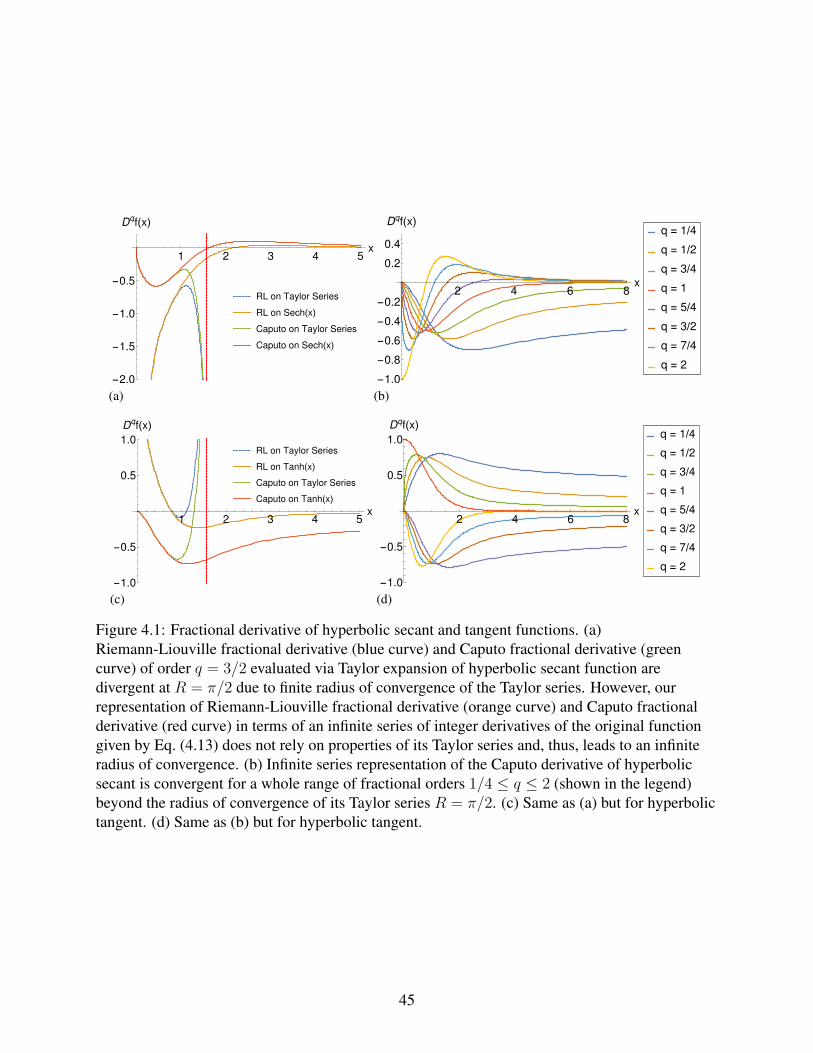
RL on Taylor Series
RL on Sech(x)
Caputo on Taylor Series
Caputo on Sech(x)
1 2 3 4 5x
-2.0
-1.5
-1.0
-0.5
Dqf(x)
(a)
2 4 6 8x
-1.0
-0.8
-0.6
-0.4
-0.2
0.2
0.4
Dqf(x)q = 1/4
q = 1/2
q = 3/4
q = 1
q = 5/4
q = 3/2
q = 7/4
q = 2
(b)
RL on Taylor Series
RL on Tanh(x)
Caputo on Taylor Series
Caputo on Tanh(x)
1 2 3 4 5x
-1.0
-0.5
0.5
1.0
Dqf(x)
(c)
2 4 6 8x
-1.0
-0.5
0.5
1.0
Dqf(x)q = 1/4
q = 1/2
q = 3/4
q = 1
q = 5/4
q = 3/2
q = 7/4
q = 2
(d)
Figure 4.1: Fractional derivative of hyperbolic secant and tangent functions. (a)Riemann-Liouville fractional derivative (blue curve) and Caputo fractional derivative (greencurve) of order q = 3/2 evaluated via Taylor expansion of hyperbolic secant function aredivergent at R = π/2 due to finite radius of convergence of the Taylor series. However, ourrepresentation of Riemann-Liouville fractional derivative (orange curve) and Caputo fractionalderivative (red curve) in terms of an infinite series of integer derivatives of the original functiongiven by Eq. (4.13) does not rely on properties of its Taylor series and, thus, leads to an infiniteradius of convergence. (b) Infinite series representation of the Caputo derivative of hyperbolicsecant is convergent for a whole range of fractional orders 1/4 ≤ q ≤ 2 (shown in the legend)beyond the radius of convergence of its Taylor series R = π/2. (c) Same as (a) but for hyperbolictangent. (d) Same as (b) but for hyperbolic tangent.
45
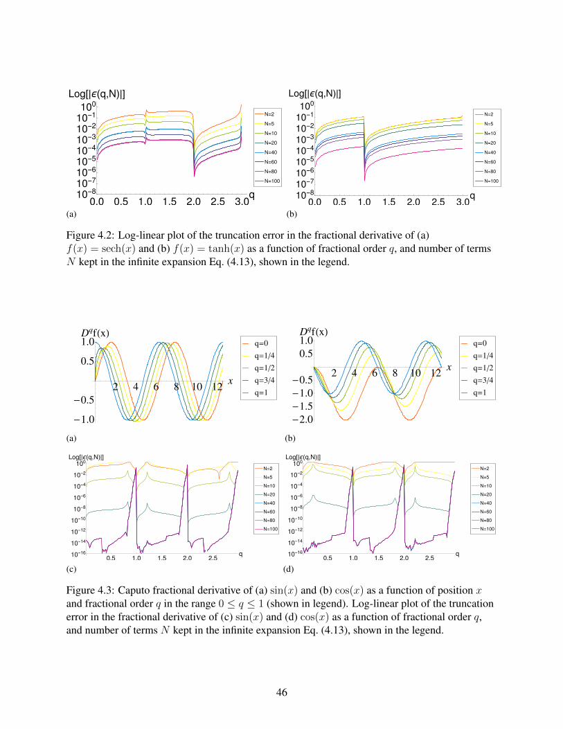
0.0 0.5 1.0 1.5 2.0 2.5 3.0q10-8
10-710-610-510-410-310-210-1100
Log[|ϵ(q,N)|]
N=100
N=80
N=60
N=40
N=20
N=10
N=5
N=2
(a)0.0 0.5 1.0 1.5 2.0 2.5 3.0
q10-810-710-610-510-410-310-210-1100
Log[|ϵ(q,N)|]
N=100
N=80
N=60
N=40
N=20
N=10
N=5
N=2
(b)
Figure 4.2: Log-linear plot of the truncation error in the fractional derivative of (a)f(x) = sech(x) and (b) f(x) = tanh(x) as a function of fractional order q, and number of termsN kept in the infinite expansion Eq. (4.13), shown in the legend.
2 4 6 8 10 12x
-1.0
-0.5
0.5
1.0DqfHxL
q=1
q=3�4
q=1�2
q=1�4
q=0
(a)
2 4 6 8 10 12x
-2.0
-1.5
-1.0
-0.5
0.5
1.0DqfHxL
q=1
q=3�4
q=1�2
q=1�4
q=0
(b)
0.5 1.0 1.5 2.0 2.5q10-16
10-14
10-12
10-10
10-8
10-6
10-4
10-2
100Log[|ϵ(q,N)|]
N=100
N=80
N=60
N=40
N=20
N=10
N=5
N=2
(c)0.5 1.0 1.5 2.0 2.5
q10-16
10-14
10-12
10-10
10-8
10-6
10-4
10-2
100Log[|ϵ(q,N)|]
N=100
N=80
N=60
N=40
N=20
N=10
N=5
N=2
(d)
Figure 4.3: Caputo fractional derivative of (a) sin(x) and (b) cos(x) as a function of position xand fractional order q in the range 0 ≤ q ≤ 1 (shown in legend). Log-linear plot of the truncationerror in the fractional derivative of (c) sin(x) and (d) cos(x) as a function of fractional order q,and number of terms N kept in the infinite expansion Eq. (4.13), shown in the legend.
46
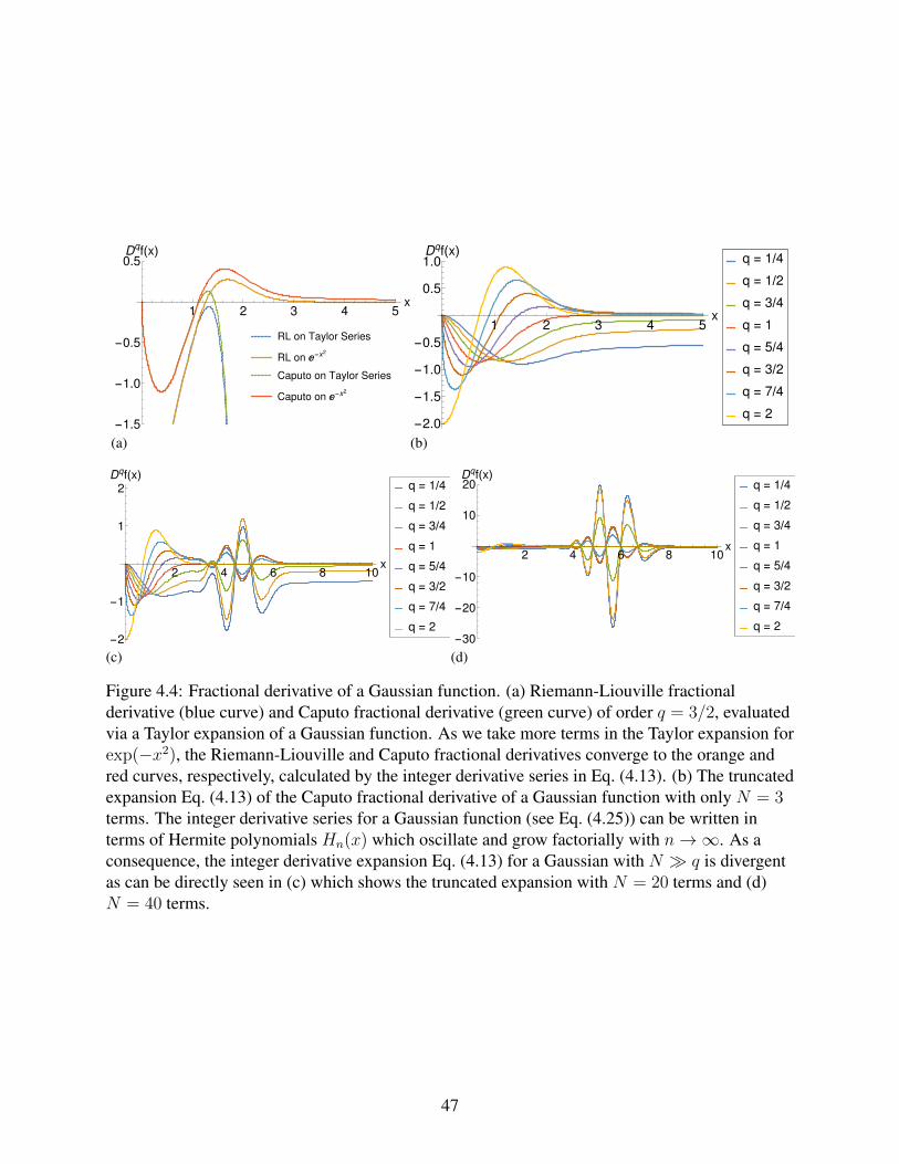
RL on Taylor Series
RL on ⅇ-x2
Caputo on Taylor Series
Caputo on ⅇ-x2
1 2 3 4 5x
-1.5
-1.0
-0.5
0.5Dqf(x)
(a)
1 2 3 4 5x
-2.0
-1.5
-1.0
-0.5
0.5
1.0Dqf(x)
q = 1/4
q = 1/2
q = 3/4
q = 1
q = 5/4
q = 3/2
q = 7/4
q = 2
(b)
2 4 6 8 10x
-2
-1
1
2Dqf(x)
q = 1/4
q = 1/2
q = 3/4
q = 1
q = 5/4
q = 3/2
q = 7/4
q = 2
(c)
2 4 6 8 10x
-30
-20
-10
10
20Dqf(x)
q = 1/4
q = 1/2
q = 3/4
q = 1
q = 5/4
q = 3/2
q = 7/4
q = 2
(d)
Figure 4.4: Fractional derivative of a Gaussian function. (a) Riemann-Liouville fractionalderivative (blue curve) and Caputo fractional derivative (green curve) of order q = 3/2, evaluatedvia a Taylor expansion of a Gaussian function. As we take more terms in the Taylor expansion forexp(−x2), the Riemann-Liouville and Caputo fractional derivatives converge to the orange andred curves, respectively, calculated by the integer derivative series in Eq. (4.13). (b) The truncatedexpansion Eq. (4.13) of the Caputo fractional derivative of a Gaussian function with only N = 3terms. The integer derivative series for a Gaussian function (see Eq. (4.25)) can be written interms of Hermite polynomials Hn(x) which oscillate and grow factorially with n→∞. As aconsequence, the integer derivative expansion Eq. (4.13) for a Gaussian with N � q is divergentas can be directly seen in (c) which shows the truncated expansion with N = 20 terms and (d)N = 40 terms.
47
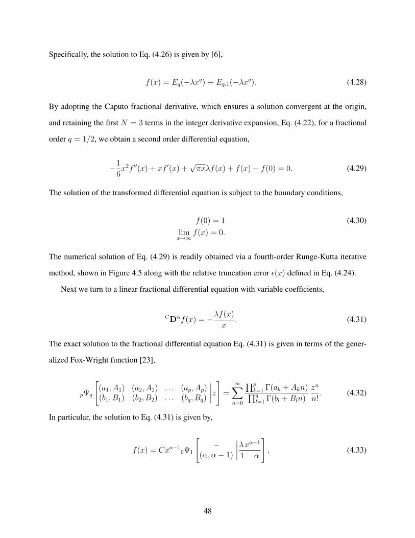
Specifically, the solution to Eq. (4.26) is given by [6],
f(x) = Eq(−λxq) ≡ Eq,1(−λxq). (4.28)
By adopting the Caputo fractional derivative, which ensures a solution convergent at the origin,
and retaining the first N = 3 terms in the integer derivative expansion, Eq. (4.22), for a fractional
order q = 1/2, we obtain a second order differential equation,
−1
6x2f ′′(x) + xf ′(x) +
√πxλf(x) + f(x)− f(0) = 0. (4.29)
The solution of the transformed differential equation is subject to the boundary conditions,
f(0) = 1 (4.30)limx→∞
f(x) = 0.
The numerical solution of Eq. (4.29) is readily obtained via a fourth-order Runge-Kutta iterative
method, shown in Figure 4.5 along with the relative truncation error ε(x) defined in Eq. (4.24).
Next we turn to a linear fractional differential equation with variable coefficients,
CDαf(x) = −λf(x)
x. (4.31)
The exact solution to the fractional differential equation Eq. (4.31) is given in terms of the gener-
alized Fox-Wright function [23],
pΨq
[(a1, A1) (a2, A2) . . . (ap, Ap)(b1, B1) (b2, B2) . . . (bq, Bq)
∣∣∣∣z]
=∞∑n=0
∏pk=1 Γ(ak + Akn)∏ql=1 Γ(bl +Bln)
zn
n!. (4.32)
In particular, the solution to Eq. (4.31) is given by,
f(x) = Cxα−10Ψ1
[−
(α, α− 1)
∣∣∣∣λxα−11− α
], (4.33)
48
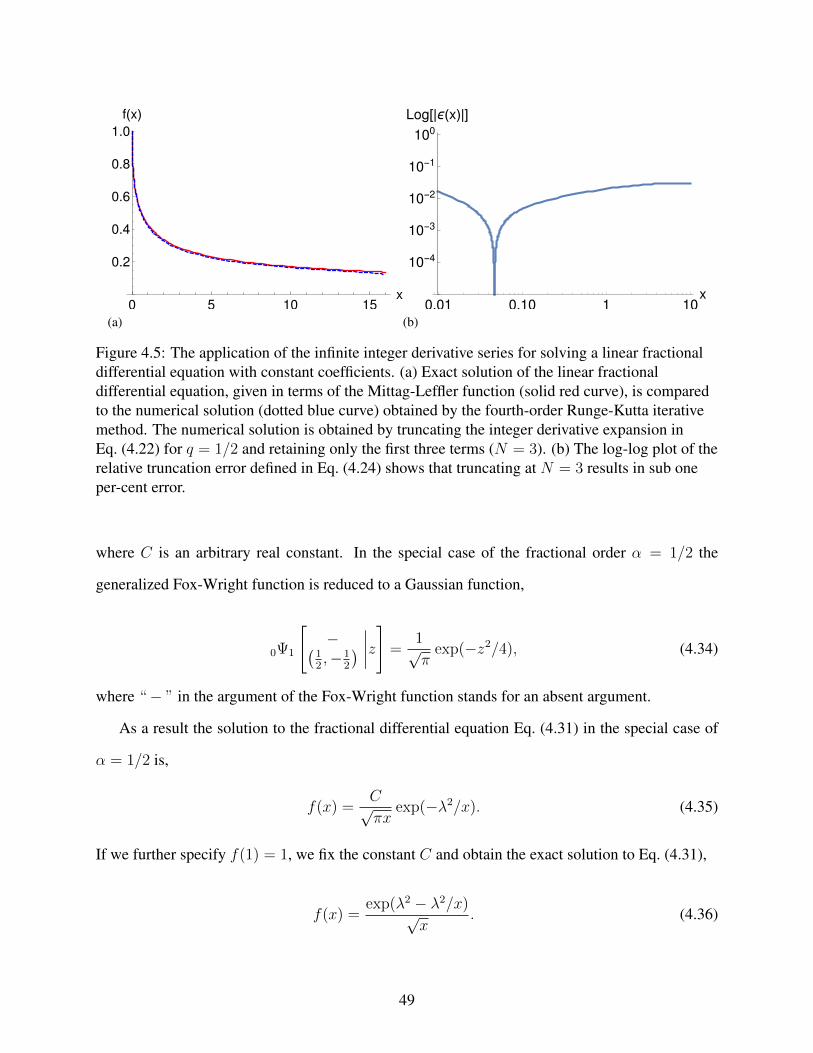
0 5 10 15x
0.2
0.4
0.6
0.8
1.0
f(x)
(a)0.01 0.10 1 10
x
10-4
10-3
10-2
10-1
100
Log[|ϵ(x)|]
(b)
Figure 4.5: The application of the infinite integer derivative series for solving a linear fractionaldifferential equation with constant coefficients. (a) Exact solution of the linear fractionaldifferential equation, given in terms of the Mittag-Leffler function (solid red curve), is comparedto the numerical solution (dotted blue curve) obtained by the fourth-order Runge-Kutta iterativemethod. The numerical solution is obtained by truncating the integer derivative expansion inEq. (4.22) for q = 1/2 and retaining only the first three terms (N = 3). (b) The log-log plot of therelative truncation error defined in Eq. (4.24) shows that truncating at N = 3 results in sub oneper-cent error.
where C is an arbitrary real constant. In the special case of the fractional order α = 1/2 the
generalized Fox-Wright function is reduced to a Gaussian function,
0Ψ1
[−(
12,−1
2
) ∣∣∣∣z]
=1√π
exp(−z2/4), (4.34)
where “− ” in the argument of the Fox-Wright function stands for an absent argument.
As a result the solution to the fractional differential equation Eq. (4.31) in the special case of
α = 1/2 is,
f(x) =C√πx
exp(−λ2/x). (4.35)
If we further specify f(1) = 1, we fix the constant C and obtain the exact solution to Eq. (4.31),
f(x) =exp(λ2 − λ2/x)√
x. (4.36)
49
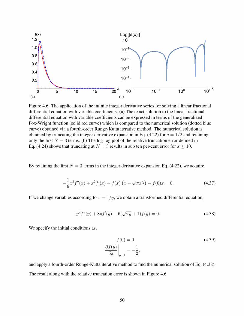
0 5 10 15 20x
0.2
0.4
0.6
0.8
1.0
1.2
f(x)
(a)10-2 10-1 100 101
x
10-4
10-3
10-2
10-1
100
Log[|ϵ(x)|]
(b)
Figure 4.6: The application of the infinite integer derivative series for solving a linear fractionaldifferential equation with variable coefficients. (a) The exact solution to the linear fractionaldifferential equation with variable coefficients can be expressed in terms of the generalizedFox-Wright function (solid red curve) which is compared to the numerical solution (dotted bluecurve) obtained via a fourth-order Runge-Kutta iterative method. The numerical solution isobtained by truncating the integer derivative expansion in Eq. (4.22) for q = 1/2 and retainingonly the first N = 3 terms. (b) The log-log plot of the relative truncation error defined inEq. (4.24) shows that truncating at N = 3 results in sub ten per-cent error for x ≤ 10.
By retaining the first N = 3 terms in the integer derivative expansion Eq. (4.22), we acquire,
−1
6x3f ′′(x) + x2f ′(x) + f(x)
(x+√πxλ
)− f(0)x = 0. (4.37)
If we change variables according to x = 1/y, we obtain a transformed differential equation,
y2f ′′(y) + 8yf ′(y)− 6(√πy + 1)f(y) = 0. (4.38)
We specify the initial conditions as,
f(0) = 0 (4.39)∂f(y)
∂x
∣∣∣∣y=1
= −1
2,
and apply a fourth-order Runge-Kutta iterative method to find the numerical solution of Eq. (4.38).
The result along with the relative truncation error is shown in Figure 4.6.
50
In this Section, we successfully demonstrated that expanding a fractional derivative in terms of
integer order derivatives is a robust method for solving linear fractional differential equations with
both constant and variable coefficients. In the special case of a differential equation with variable
coefficients, the truncated series with only the firstN = 3 terms leads to a 10% error, while the very
same truncation applied to a differential equation with constant coefficients results in a 1% error.
Although this method cannot be exhaustively tested for all possible fractional orders of differential
operators and all types of FDEs, linear FDEs, considered in this work, constitute a large sample
that can be used in many physical applications where the response of a system is proportional to a
fractional order parameter [6, 7, 29]. Thus, the numerical scheme based on the truncated integer
derivative expansion is a powerful method for solving a broad range of linear FDEs.
4.6 Conclusions
In this paper we expressed the Grunwald-Letnikov fractional derivative as an infinite sum of
integer order derivatives. We compared the obtained infinite expansion with the corresponding
series produced by the Riemann-Liouville and Caputo definitions of a fractional derivative. We
found that all three definitions are represented by the very same infinite series, with the excep-
tion of the lower index of summation for the Caputo fractional derivative which accounts for the
initial conditions at the expansion point. Thus, we have shown that the integer derivative series
representation provides a unified description for various definitions of a fractional derivative.
By truncating the infinite expansion and retaining only the first few terms, we demonstrated the
convergence of the Grunwald-Letnikov fractional derivative. We have shown that for functions rep-
resented by Taylor series with an infinite radius of convergence, the truncation error decreases with
an increasing number of terms kept in the truncated expansion. We emphasized that the infinite
expansion does not rely on the properties of the Taylor series, which has profound consequences
for the functions characterized by a finite radius of convergence of the corresponding Taylor series.
Specifically, we have shown that the infinite series of integer order derivatives for hyperbolic secant
and tangent functions has an infinite radius of convergence, compared to the corresponding Taylor
51
series with a finite radius of convergence of π/2. However, for a Gaussian function we found that
the infinite expansion is divergent due to the factorial growth and oscillatory nature of the Her-
mite polynomials. Thus, the Gaussian function establishes limits of the universality of the infinite
expansion of the Grunwald-Letnikov fractional derivative in terms of integer order derivatives.
Finally, we applied the truncated series for a fractional derivative to solve linear fractional dif-
ferential equations with both constant and variable coefficients. We found that the fourth-order
Runge-Kutta method applied to truncated fractional differential equations results in numerical so-
lutions that rapidly converge to the exact solutions given in terms of Mittag-Leffler and generalized
Fox-Wright special functions. Thus, we concluded that the integer derivative expansion can be
adapted to a robust numerical method for solving linear fractional differential equations, such as
the fractional Schrodinger and fractional diffusion equations.
52
CHAPTER 5
EXACT RESULTS FOR A FRACTIONAL DERIVATIVE OF ELEMENTARY FUNCTIONS
A paper accepted for publication in SciPost Physics, arXiv:1711.07126† (2017) [11]
Gavriil Shchedrin*, Nathanael C. Smith*, Anastasia Gladkina*, and Lincoln D. Carr*
We present exact analytical results for the Caputo fractional derivative of a wide class of ele-
mentary functions, including trigonometric and inverse trigonometric, hyperbolic and inverse hy-
perbolic, Gaussian, quartic Gaussian, and Lorentzian functions. These results are especially im-
portant for multiscale physical systems, such as porous materials, disordered media, and turbulent
fluids, in which transport is described by fractional partial differential equations. The exact results
for the Caputo fractional derivative are obtained from a single generalized Euler’s integral trans-
form of the generalized hypergeometric function with a power-law argument. We present a proof
of the generalized Euler’s integral transform and directly apply it to the exact evaluation of the
Caputo fractional derivative of a broad spectrum of functions, provided that these functions can
be expressed in terms of a generalized hypergeometric function with a power-law argument. We
determine that the Caputo fractional derivative of elementary functions is given by the generalized
hypergeometric function. Moreover, we show that in the most general case the final result cannot
be reduced to elementary functions, in contrast to both the Liouville-Caputo and Fourier fractional
derivatives. However, we establish that in the infinite limit of the argument of elementary func-
tions, all three definitions of a fractional derivative – the Caputo, Liouville-Caputo, and Fourier –
converge to the same result given by the elementary functions. Finally, we prove the equivalence
between Liouville-Caputo and Fourier fractional derivatives.
5.1 Introduction
The notion of a fractional derivative and fractional integral of any order, real or complex, is
a profound concept in calculus, complex analysis, and the theory of integro-differential equations†Permission is provided by the Creative Commons Attribution 4.0 International License used for this publication.*Department of Physics, Colorado School of Mines.
53
[14, 23]. These fractional operators have unique mathematical properties and remarkable rela-
tions to special functions and integral transforms [33–36]. Apart from its applications in pure
mathematics and mathematical physics, the notion of a fractional derivative has found a number
of applications in fundamental and applied physics [6]. Indeed, transport phenomena in a wide
class of multiscale physical systems, such as porous materials, disordered media, and turbulent
fluids are described by the fractional diffusion equation [4, 37, 38]. Only within the framework
of fractional partial differential equations can the properties of multiscale physical systems, such
as non-Gaussian statistics, non-Fickian transport, nonlocality, fractional geometry, and long-range
correlations, be taken into account in a simple, unified, and systematic way [6, 7]. The optimal
transport through the living porous systems, such as animal tissues and leaves that are made of
a highly sophisticated hierarchical network of pores and tubes, is governed by the Murray’s law
[39–45]. Recently, Murray’s law was successfully used to design synthetic materials, which allow
one to achieve an enhanced transfer rate and mass exchange with applications that range from fast
gas detection sensors to highly efficient electrical batteries [46]. Furthermore, it was shown that
living systems, such as neural clusters and heart cell arrays exhibit multiple time scales of adapta-
tion, which, in turn, are governed by a fractional derivative of slowly varying stimulus parameters
[30, 31].
The progress in both fundamental and mathematical physics is heavily influenced by integrable
models, such as the hydrogen atom and harmonic oscillator, the evolution of which is governed by
partial differential equations (PDEs). Naturally, exact results in fractional PDEs [47–50] give deep
insight into physics that govern systems characterized by multiple spatial and temporal scales.
The central object in fractional PDEs is a fractional derivative, which can be defined in various
ways [6, 23]. Among the multiplex of fractional derivatives, the Caputo fractional derivative [6,
23, 51] has been proven the most effective in physical applications [6]. Powerful exact methods
and numerical techniques were developed that allowed one to evaluate fractional derivatives of a
wide class of functions [14, 23, 33, 36, 47–50, 52–65]. However, these methods did not provide
a single and universal method that could be used in finding exact expressions for the Caputo
54
fractional derivative of elementary functions, such as the Gaussian, Lorentzian, trigonometric and
hyperbolic functions, which play a paramount role in physical applications [6]. In this paper,
we construct a single method based on the generalized Euler’s integral transform that enables the
exact evaluation of the Caputo fractional derivative of a broad spectrum of elementary functions,
provided that these functions can be expressed in terms of the generalized hypergeometric function
with a power-law argument. We compare the obtained results for the Caputo fractional derivative
with the Liouville-Caputo and Fourier fractional derivatives. Specifically, we show that the Caputo
fractional derivative of elementary is given in terms of the generalized hypergeometric function,
which in the most general case, cannot be reduced to elementary functions, in contrast to both the
Liouville-Caputo and Fourier fractional derivatives. However, we find that in the infinite limit of
the argument of elementary functions all three definitions of a fractional derivative – the Caputo,
Liouville-Caputo, and Fourier – converge to the same result. Moreover, we establish the complete
equivalence between the Liouville-Caputo and Fourier fractional derivative, despite the fact that
the latter derivative is defined in the momentum space while the former derivative is defined in the
configuration space.
The rest of this paper has the following organization. In Section 5.2 we introduce the main
idea that allows us to translate the Caputo fractional derivative into the generalized Euler’s inte-
gral transform (EIT). In Section 5.3 we present the proof of the generalized EIT. The consecutive
Sections 5.4 to 5.7 present direct implementation of the generalized EIT for the specific case of
the Caputo fractional derivative of trigonometric and inverse trigonometric, hyperbolic and inverse
hyperbolic, Gaussian, quartic Gaussian, and Lorentzian functions, correspondingly. Section 5.8
introduces the Liouville-Caputo and Fourier fractional derivatives and shows the complete equiv-
alence between them. Finally, in Section 5.9 we present the correspondence between the Caputo,
Liouville-Caputo, and Fourier fractional derivatives.
55
5.2 The main idea in a nutshell
In this Section we define the Caputo fractional derivative and formulate it in terms of the gen-
eralized Euler’s integral transform (EIT). This transform formulates a definite integral of the beta-
type distribution multiplied by the hypergeometric function with polynomial argument in terms of
a single hypergeometric function of a higher order. The transformation of an elementary function
into the generalized hypergeometric function enables us to formulate the Caputo fractional deriva-
tive in terms of the generalized Euler’s integral transform. The EIT effectively transforms the
Caputo fractional derivative into a system of linear equations, which can be readily solved. Thus,
we obtain an exact analytical result for the Caputo fractional derivative of a wide class of elemen-
tary functions, provided that they can be expressed in terms of the generalized hypergeometric
function with a polynomial argument.
The Caputo fractional derivative of a fractional order 0 < α < 1 is defined as [14, 23],
CDαxf(x) =
1
Γ(1− α)
∫ x
0
dt (x− t)−α df(t)
dt. (5.1)
First, we notice that many elementary functions and their derivatives can be expressed in terms of
the generalized hypergeometric function AFB, e.g. [19, 66],
sin(x) = x 0F1
[; 3/2;−x2/4
]exp(−x2) = 1F1
[1; 1;−x2
]. (5.2)
Next, we perform a re-scaling of the argument, t → xt, in Eq. (5.1), and express an elementary
function f(x) in terms of a generalized hypergeometric function. Thus, we can represent the
Caputo fractional derivative in Eq. (5.1) of an elementary function f(x) in terms of the integral
transform,
CDαxf(x) = g(α, x)
∫ 1
0
dt tc−1 (1− t)d−c−1 AFB
a1, . . . , aA
b1, . . . , bB
; ztm
, (5.3)
56
where the arrays of constants (a1 · · · aA) ≡ ~a and (b1 · · · bB) ≡ ~b in the argument of the generalized
hypergeometric function AFB
(~a,~b; ztm
), along with constants c, d, m, and functions g(α, x) and
z = z(x) depend on the specific choice of the function f(x), fractional order α, and argument x. In
this paper we will restrict our choice to the integer powers of the argument of the hypergeometric
function, i.e., m ∈ N. The integral representation given by Eq. (5.3) of the Caputo fractional
derivative originally defined by Eq. (5.1) is nothing but the generalized EIT, as compared to the
conventional EIT, given by [67–69],
A+1FB+1
a1, . . . , aA, c
b1, . . . , bB, d; z
= (5.4)
=Γ(d)
Γ(c)Γ(d− c)
∫ 1
0
dt tc−1 (1− t)d−c−1 AFB
a1, . . . , aA
b1, . . . , bB
; zt
. (5.5)
We shall note, however, that the Caputo fractional derivative of elementary functions involves the
generalized hypergeometric function with a power-law argument in contrast to the conventional
EIT given by Eq. (5.4), which is formulated in terms of the generalized hypergeometric function
with a linear argument. In the next Section we prove that the generalized EIT for the hypergeo-
metric function with a power-law argument is given in terms of a single hypergeometric function
of a higher order. This will allow us to obtain exact analytical results for the Caputo fractional
derivative of a broad class of elementary functions, including, but not limited to, trigonometric
and inverse trigonometric, hyperbolic and inverse hyperbolic, Gaussian, quartic Gaussian, and
Lorentzian functions. Even though we restricted the order of the Caputo fractional derivative to
be 0 < α < 1, the obtained results could be easily extended to a general case 0 ≤ α ≤ ∞ by
employing the semi-group property of a fractional derivative [14, 23, 33].
57
5.3 Generalized Euler’s integral transform of the hypergeometric function with a power-law argument
In the previous Section we have transformed the Caputo fractional derivative into the general-
ized Euler’s integral transform (EIT) of the hypergeometric function with a power-law argument.
The goal of this Section is to derive the generalized EIT of the hypergeometric function with a
power-law argument in terms of the hypergeometric function of a higher order. Specifically, we
will prove the following result that holds for the generalized EIT,
A+mFB+m
a1, . . . , aA, c0, . . . cm−1
b1, . . . , bB, d0, . . . dm−1
; z
= (5.6)
=Γ(d)
Γ(d− c)Γ(c)
∫ 1
0
dt tc−1 (1− t)d−c−1 AFB
a1, . . . , aA
b1, . . . , bB
; ztm
,where the constants cj and dj are given by cj = (c+ j)/m, and dj = (d+ j)/m with index j
spanning j ∈ [0, 1, · · · ,m− 1].
We begin the proof of Eq. (5.6) by considering the integral,
AJB =
∫ 1
0
dt tc−1 (1− t)d−c−1 AFB
[a1, . . . , aAb1, . . . , bB
; ztm
]. (5.7)
First, we expand the hypergeometric function in the hypergeometric series,
AJB =∞∑n=0
(a1)n · · · (aA)n(b1)n · · · (bB)n
zn
n!
∫ 1
0
dt tc−1 (1− t)d−c−1 tmn, (5.8)
where (a)n is the Pochhammer symbol [19, 70],
(a)n =Γ(a+ n)
Γ(a), (5.9)
and Γ(z) is the Euler’s gamma function. The definite integral, which appears in Eq. (5.8), can be
readily evaluated and we obtain,
58
I ≡∫ 1
0
dt tc−1 (1− t)d−c−1 tmn =Γ(d− c)Γ(c+mn)
Γ(d+mn)
=Γ(d− c)Γ(c)
Γ(d)
Γ(c+mn)
Γ(c)
(Γ(d+mn)
Γ(d)
)−1=
Γ(d− c)Γ(c)
Γ(d)
(c)mn(d)mn
. (5.10)
For integer values m ∈ N we can use the multiplication property of the Pochhammer symbol [70],
i.e.
(a)k+mn = (a)kmmn
m−1∏j=0
(a+ j + k
m
)n
. (5.11)
In our special case we have zero offset k = 0, which simplifies the Pochhammer symbol into,
(a)mn = mmn
m−1∏j=0
(a+ j
m
)n
. (5.12)
Thus, the integral given by Eq. (5.10) can be expressed in terms of the product of ratios of
Pochhammer symbols,
I =Γ(d− c)Γ(c)
Γ(d)
∏m−1j=0
(c+jm
)n∏m−1
j=0
(d+jm
)n
. (5.13)
The form of the integral in Eq. (5.13) is particularly convenient for the evaluation of the sum in
Eq. (5.8), which results in the generalized hypergeometric function of a higher order,
AJB =Γ(d− c)Γ(c)
Γ(d)
∞∑n=0
(a1)n · · · (aA)n(b1)n · · · (bB)n
∏m−1j=0
(c+jm
)n∏m−1
j=0
(d+jm
)n
zn
n!
=Γ(d− c)Γ(c)
Γ(d)A+mFB+m
[a1, . . . , aA, c0, . . . cm−1b1, . . . , bB, d0, . . . dm−1
; z
], (5.14)
where the constants cj and dj are given by cj = (c+ j)/m, and dj = (d+ j)/m with index
spanning j ∈ [0, 1, . . . ,m − 1]. The comparison between Eq. (5.7) and Eq. (5.14) finishes the
59
proof of the main result given by Eq. (5.6). Thus, we have shown that the generalized EIT of the
hypergeometric function with power-law argument is a hypergeometric function of a higher order.
5.4 Fractional derivative of trigonometric functions
In Sections 5.1 and 5.2 we have formulated the Caputo fractional derivative in terms of the
generalized EIT and derived the main result for the generalized EIT of a hypergeometric function
with a power-law argument. The goal of this Section, as well as Sections 5.4 to 5.8, is to apply the
main result in Eq. (5.6) for the exact evaluation of the Caputo fractional derivative of a wide class
of elementary functions. Specifically, in this Section we obtain the Caputo fractional derivative of
trigonometric and hyperbolic functions by means of the generalized EIT. We begin with the Caputo
fractional derivative of f(x) = sin[(βx)n
]with integer power n ∈ N,
CDαx
(sin[(βx)n]
)= (5.15)
=nβn
Γ(1− α)
∫ x
0
dt (x− t)−α tn−1 cos[(βt)n]
=nβnxn−α
Γ(1− α)
∫ 1
0
dt (1− t)−α tn−1 cos[(βxt)n]
=nβnxn−α
Γ(1− α)
∫ 1
0
dt (1− t)−α tn−1 0F1
[;1
2;−(βxt)2n
4
].
Unless otherwise stated, we set β to be a constant parameter. In derivation of Eq. (5.15) we
expressed cosine in terms of the hypergeometric function Eq. (5.2),
cos[(βx)n] = 0F1
[;1
2;−(βx)2n
4
]. (5.16)
By comparing the general result Eq. (5.6) with the right-hand side of Eq. (5.15) we obtain a system
of linear equations for the variables c, d,m, and z in terms of integer power n and fractional
60
parameter α,
m = 2n (5.17)
c− 1 = n− 1 (5.18)
d− c− 1 = −α (5.19)
z = −(βx)2n
4, (5.20)
which can be readily solved, yielding c = n, d = n+ 1−α. Thus we obtain the Caputo fractional
derivative of sine (see Figure 5.1a),
CDαx
(sin[(βx)n]
)= βnxn−α
Γ(n+ 1)
Γ(n+ 1− α)× (5.21)
×2nF2n+1
n/2n, (n+ 1)/2n, · · · (3n− 1)/2n
1/2, (n+ 1− α)/2n, · · · (3n− α)/2n;−(βx)2n
4
= βnxn−α
Γ(n+ 1)
Γ(n+ 1− α)2n−1F2n
(n+ 1)/2n, · · · (3n− 1)/2n
(n+ 1− α)/2n, · · · (3n− α)/2n;−(βx)2n
4
.In the special case of n = 1 the general form of the Caputo fractional derivative can be simplified
to [6, 14],
CDαx
[sin(βx)
]=
βx1−α
Γ(2− α)1F2
[1
(2− α)/2, (3− α)/2;−β
2x2
4
]. (5.22)
61
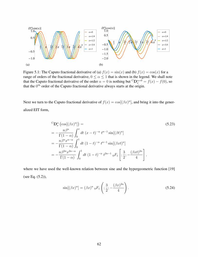
Π
2Π
3 Π
22 Π
5 Π
23 Π
7 Π
24 Π
x
-1.0
-0.5
0.5
1.0Dx
Α@sinHxLD
Α=1
Α=3�4
Α=1�2
Α=1�4
Α=0
(a)
Π
2Π
3 Π
22 Π
5 Π
23 Π
7 Π
24 Π
x
-2.0
-1.5
-1.0
-0.5
0.5
1.0Dx
Α@cosHxLD
Α=1
Α=3�4
Α=1�2
Α=1�4
Α=0
(b)
Figure 5.1: The Caputo fractional derivative of (a) f(x) = sin(x) and (b) f(x) = cos(x) for arange of orders of the fractional derivative, 0 ≤ α ≤ 1 that is shown in the legend. We shall notethat the Caputo fractional derivative of the order α = 0 is nothing but CDα=0
x = f(x)− f(0), sothat the 0th order of the Caputo fractional derivative always starts at the origin.
Next we turn to the Caputo fractional derivative of f(x) = cos[(βx)n], and bring it into the gener-
alized EIT form,
CDαx
(cos[(βx)n]
)= (5.23)
= − nβn
Γ(1− α)
∫ x
0
dt (x− t)−α tn−1 sin[(βt)n]
= −nβnxn−α
Γ(1− α)
∫ 1
0
dt (1− t)−α tn−1 sin[(βxt)n]
= −nβ2nx2n−α
Γ(1− α)
∫ 1
0
dt (1− t)−α t2n−1 0F1
[;3
2;−(βxt)2n
4
],
where we have used the well-known relation between sine and the hypergeometric function [19]
(see Eq. (5.2)),
sin[(βx)n] = (βx)n 0F1
(;3
2;−(βx)2n
4
). (5.24)
62
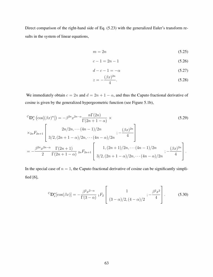
Direct comparison of the right-hand side of Eq. (5.23) with the generalized Euler’s transform re-
sults in the system of linear equations,
m = 2n (5.25)
c− 1 = 2n− 1 (5.26)
d− c− 1 = −α (5.27)
z = −(βx)2n
4. (5.28)
We immediately obtain c = 2n and d = 2n + 1− α, and thus the Caputo fractional derivative of
cosine is given by the generalized hypergeometric function (see Figure 5.1b),
CDαx
(cos[(βx)n]
)= −β2nx2n−α
nΓ(2n)
Γ(2n+ 1− α)× (5.29)
×2nF2n+1
2n/2n, · · · (4n− 1)/2n
3/2, (2n+ 1− α)/2n, · · · (4n− α)/2n;−(βx)2n
4
= −β
2nx2n−α
2
Γ(2n+ 1)
Γ(2n+ 1− α)2nF2n+1
1, (2n+ 1)/2n, · · · (4n− 1)/2n
3/2, (2n+ 1− α)/2n, · · · (4n− α)/2n;−(βx)2n
4
.In the special case of n = 1, the Caputo fractional derivative of cosine can be significantly simpli-
fied [6],
CDαx [cos(βx)] = − β2x2−α
Γ(3− α)1F2
1
(3− α)/2, (4− α)/2;−β
2x2
4
. (5.30)
63
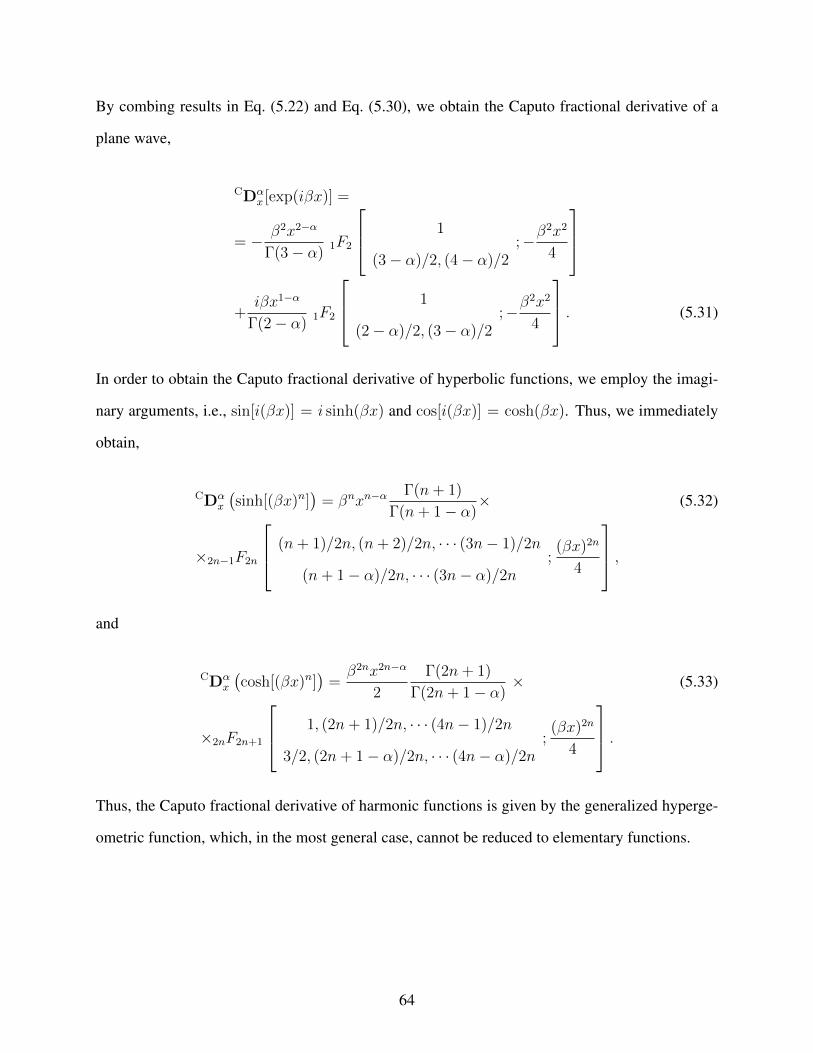
By combing results in Eq. (5.22) and Eq. (5.30), we obtain the Caputo fractional derivative of a
plane wave,
CDαx [exp(iβx)] =
= − β2x2−α
Γ(3− α)1F2
1
(3− α)/2, (4− α)/2;−β
2x2
4
+iβx1−α
Γ(2− α)1F2
1
(2− α)/2, (3− α)/2;−β
2x2
4
. (5.31)
In order to obtain the Caputo fractional derivative of hyperbolic functions, we employ the imagi-
nary arguments, i.e., sin[i(βx)] = i sinh(βx) and cos[i(βx)] = cosh(βx). Thus, we immediately
obtain,
CDαx
(sinh[(βx)n]
)= βnxn−α
Γ(n+ 1)
Γ(n+ 1− α)× (5.32)
×2n−1F2n
(n+ 1)/2n, (n+ 2)/2n, · · · (3n− 1)/2n
(n+ 1− α)/2n, · · · (3n− α)/2n;(βx)2n
4
,and
CDαx
(cosh[(βx)n]
)=β2nx2n−α
2
Γ(2n+ 1)
Γ(2n+ 1− α)× (5.33)
×2nF2n+1
1, (2n+ 1)/2n, · · · (4n− 1)/2n
3/2, (2n+ 1− α)/2n, · · · (4n− α)/2n;(βx)2n
4
.Thus, the Caputo fractional derivative of harmonic functions is given by the generalized hyperge-
ometric function, which, in the most general case, cannot be reduced to elementary functions.
64
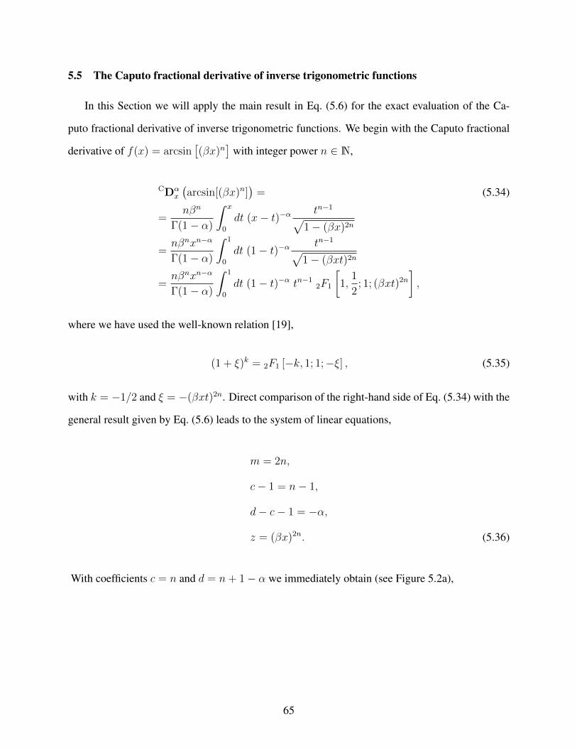
5.5 The Caputo fractional derivative of inverse trigonometric functions
In this Section we will apply the main result in Eq. (5.6) for the exact evaluation of the Ca-
puto fractional derivative of inverse trigonometric functions. We begin with the Caputo fractional
derivative of f(x) = arcsin[(βx)n
]with integer power n ∈ N,
CDαx
(arcsin[(βx)n]
)= (5.34)
=nβn
Γ(1− α)
∫ x
0
dt (x− t)−α tn−1√1− (βx)2n
=nβnxn−α
Γ(1− α)
∫ 1
0
dt (1− t)−α tn−1√1− (βxt)2n
=nβnxn−α
Γ(1− α)
∫ 1
0
dt (1− t)−α tn−1 2F1
[1,
1
2; 1; (βxt)2n
],
where we have used the well-known relation [19],
(1 + ξ)k = 2F1 [−k, 1; 1;−ξ] , (5.35)
with k = −1/2 and ξ = −(βxt)2n. Direct comparison of the right-hand side of Eq. (5.34) with the
general result given by Eq. (5.6) leads to the system of linear equations,
m = 2n,
c− 1 = n− 1,
d− c− 1 = −α,
z = (βx)2n. (5.36)
With coefficients c = n and d = n+ 1− α we immediately obtain (see Figure 5.2a),
65
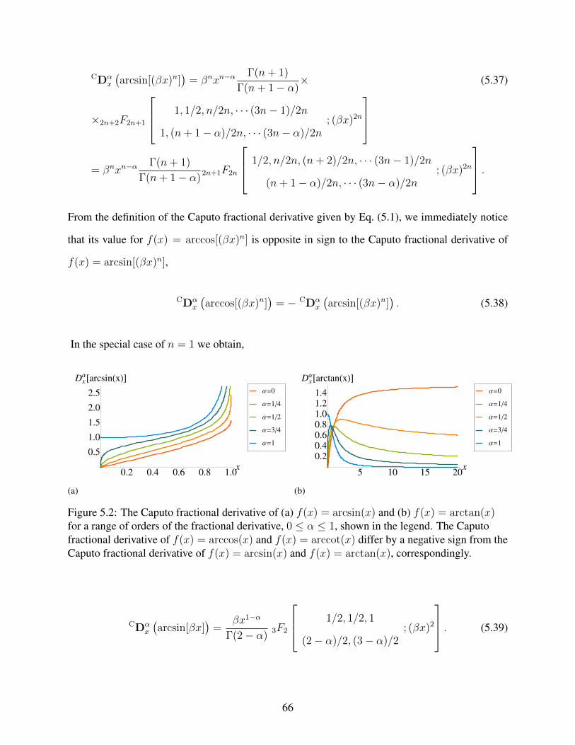
CDαx
(arcsin[(βx)n]
)= βnxn−α
Γ(n+ 1)
Γ(n+ 1− α)× (5.37)
×2n+2F2n+1
1, 1/2, n/2n, · · · (3n− 1)/2n
1, (n+ 1− α)/2n, · · · (3n− α)/2n; (βx)2n
= βnxn−α
Γ(n+ 1)
Γ(n+ 1− α)2n+1F2n
1/2, n/2n, (n+ 2)/2n, · · · (3n− 1)/2n
(n+ 1− α)/2n, · · · (3n− α)/2n; (βx)2n
.From the definition of the Caputo fractional derivative given by Eq. (5.1), we immediately notice
that its value for f(x) = arccos[(βx)n] is opposite in sign to the Caputo fractional derivative of
f(x) = arcsin[(βx)n],
CDαx
(arccos[(βx)n]
)= − CDα
x
(arcsin[(βx)n]
). (5.38)
In the special case of n = 1 we obtain,
0.2 0.4 0.6 0.8 1.0x
0.5
1.0
1.5
2.0
2.5
Dx
Α@arcsinHxLD
Α=1
Α=3�4
Α=1�2
Α=1�4
Α=0
(a)
5 10 15 20x
0.2
0.4
0.6
0.8
1.0
1.2
1.4
Dx
Α@arctanHxLD
Α=1
Α=3�4
Α=1�2
Α=1�4
Α=0
(b)
Figure 5.2: The Caputo fractional derivative of (a) f(x) = arcsin(x) and (b) f(x) = arctan(x)for a range of orders of the fractional derivative, 0 ≤ α ≤ 1, shown in the legend. The Caputofractional derivative of f(x) = arccos(x) and f(x) = arccot(x) differ by a negative sign from theCaputo fractional derivative of f(x) = arcsin(x) and f(x) = arctan(x), correspondingly.
CDαx
(arcsin[βx]
)=
βx1−α
Γ(2− α)3F2
1/2, 1/2, 1
(2− α)/2, (3− α)/2; (βx)2
. (5.39)
66
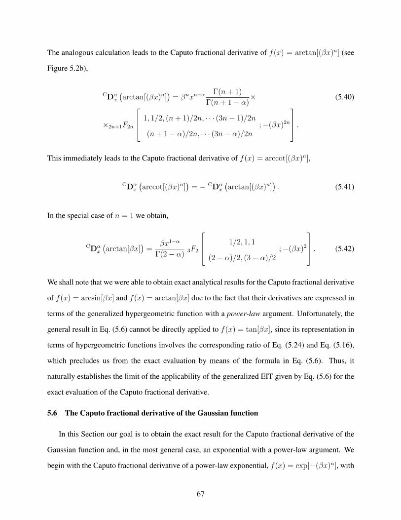
The analogous calculation leads to the Caputo fractional derivative of f(x) = arctan[(βx)n] (see
Figure 5.2b),
CDαx
(arctan[(βx)n]
)= βnxn−α
Γ(n+ 1)
Γ(n+ 1− α)× (5.40)
×2n+1F2n
1, 1/2, (n+ 1)/2n, · · · (3n− 1)/2n
(n+ 1− α)/2n, · · · (3n− α)/2n;−(βx)2n
.This immediately leads to the Caputo fractional derivative of f(x) = arccot[(βx)n],
CDαx
(arccot[(βx)n]
)= − CDα
x
(arctan[(βx)n]
). (5.41)
In the special case of n = 1 we obtain,
CDαx
(arctan[βx]
)=
βx1−α
Γ(2− α)3F2
1/2, 1, 1
(2− α)/2, (3− α)/2;−(βx)2
. (5.42)
We shall note that we were able to obtain exact analytical results for the Caputo fractional derivative
of f(x) = arcsin[βx] and f(x) = arctan[βx] due to the fact that their derivatives are expressed in
terms of the generalized hypergeometric function with a power-law argument. Unfortunately, the
general result in Eq. (5.6) cannot be directly applied to f(x) = tan[βx], since its representation in
terms of hypergeometric functions involves the corresponding ratio of Eq. (5.24) and Eq. (5.16),
which precludes us from the exact evaluation by means of the formula in Eq. (5.6). Thus, it
naturally establishes the limit of the applicability of the generalized EIT given by Eq. (5.6) for the
exact evaluation of the Caputo fractional derivative.
5.6 The Caputo fractional derivative of the Gaussian function
In this Section our goal is to obtain the exact result for the Caputo fractional derivative of the
Gaussian function and, in the most general case, an exponential with a power-law argument. We
begin with the Caputo fractional derivative of a power-law exponential, f(x) = exp[−(βx)n], with
67
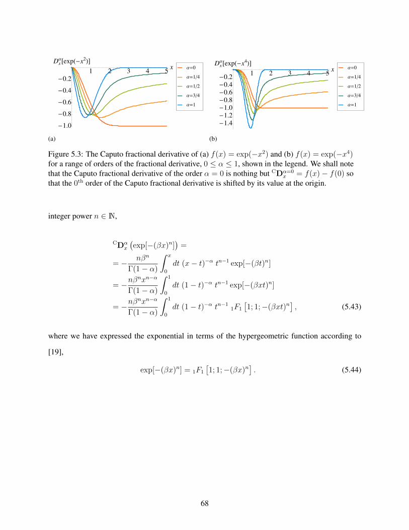
1 2 3 4 5x
-1.0
-0.8
-0.6
-0.4
-0.2
Dx
Α@expH-x2LD
Α=1
Α=3�4
Α=1�2
Α=1�4
Α=0
(a)
1 2 3 4 5x
-1.4-1.2-1.0-0.8-0.6-0.4-0.2
Dx
Α@expH-x4LD
Α=1
Α=3�4
Α=1�2
Α=1�4
Α=0
(b)
Figure 5.3: The Caputo fractional derivative of (a) f(x) = exp(−x2) and (b) f(x) = exp(−x4)for a range of orders of the fractional derivative, 0 ≤ α ≤ 1, shown in the legend. We shall notethat the Caputo fractional derivative of the order α = 0 is nothing but CDα=0
x = f(x)− f(0) sothat the 0th order of the Caputo fractional derivative is shifted by its value at the origin.
integer power n ∈ N,
CDαx
(exp[−(βx)n]
)=
= − nβn
Γ(1− α)
∫ x
0
dt (x− t)−α tn−1 exp[−(βt)n]
= −nβnxn−α
Γ(1− α)
∫ 1
0
dt (1− t)−α tn−1 exp[−(βxt)n]
= −nβnxn−α
Γ(1− α)
∫ 1
0
dt (1− t)−α tn−1 1F1
[1; 1;−(βxt)n
], (5.43)
where we have expressed the exponential in terms of the hypergeometric function according to
[19],
exp[−(βx)n] = 1F1
[1; 1;−(βx)n
]. (5.44)
68
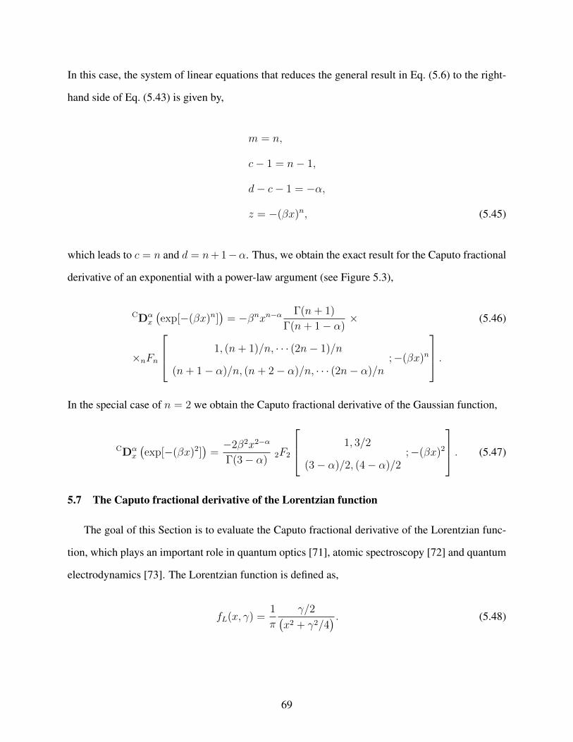
In this case, the system of linear equations that reduces the general result in Eq. (5.6) to the right-
hand side of Eq. (5.43) is given by,
m = n,
c− 1 = n− 1,
d− c− 1 = −α,
z = −(βx)n, (5.45)
which leads to c = n and d = n+ 1−α. Thus, we obtain the exact result for the Caputo fractional
derivative of an exponential with a power-law argument (see Figure 5.3),
CDαx
(exp[−(βx)n]
)= −βnxn−α Γ(n+ 1)
Γ(n+ 1− α)× (5.46)
×nFn
1, (n+ 1)/n, · · · (2n− 1)/n
(n+ 1− α)/n, (n+ 2− α)/n, · · · (2n− α)/n;−(βx)n
.In the special case of n = 2 we obtain the Caputo fractional derivative of the Gaussian function,
CDαx
(exp[−(βx)2]
)=−2β2x2−α
Γ(3− α)2F2
1, 3/2
(3− α)/2, (4− α)/2;−(βx)2
. (5.47)
5.7 The Caputo fractional derivative of the Lorentzian function
The goal of this Section is to evaluate the Caputo fractional derivative of the Lorentzian func-
tion, which plays an important role in quantum optics [71], atomic spectroscopy [72] and quantum
electrodynamics [73]. The Lorentzian function is defined as,
fL(x, γ) =1
π
γ/2(x2 + γ2/4
) . (5.48)
69
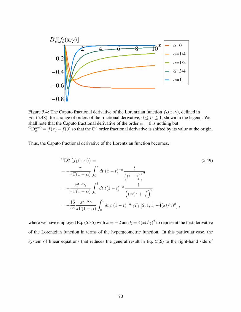
2 4 6 8 10x
-0.8
-0.6
-0.4
-0.2
DxΑ@ fLHx,ΓLD
Α=1
Α=3�4
Α=1�2
Α=1�4
Α=0
Figure 5.4: The Caputo fractional derivative of the Lorentzian function fL(x, γ), defined inEq. (5.48), for a range of orders of the fractional derivative, 0 ≤ α ≤ 1, shown in the legend. Weshall note that the Caputo fractional derivative of the order α = 0 is nothing butCDα=0
x = f(x)− f(0) so that the 0th order fractional derivative is shifted by its value at the origin.
Thus, the Caputo fractional derivative of the Lorentzian function becomes,
CDαx
(fL(x, γ)
)= (5.49)
= − γ
πΓ(1− α)
∫ x
0
dt (x− t)−α t(t2 + γ2
4
)2= − x2−αγ
πΓ(1− α)
∫ 1
0
dt t(1− t)−α 1((xt)2 + γ2
4
)2= −16
γ4x2−αγ
πΓ(1− α)
∫ 1
0
dt t (1− t)−α 2F1
[2, 1; 1;−4(xt/γ)2
],
where we have employed Eq. (5.35) with k = −2 and ξ = 4(xt/γ)2 to represent the first derivative
of the Lorentzian function in terms of the hypergeometric function. In this particular case, the
system of linear equations that reduces the general result in Eq. (5.6) to the right-hand side of
70
Eq. (5.43) is given by,
m = 2,
c− 1 = 1,
d− c− 1 = −α,
z = −4(x/γ)2, (5.50)
which leads to c = 2 and d = 3 − α. Thus, we obtain the exact result for the Caputo fractional
derivative of the Lorentzian function (see Figure 5.4),
CDαx
(fL(x, γ)
)= − 16x2−α
πγ3 Γ(3− α)3F2
1, 3/2, 2
(3− α)/2, (4− α)/2;−4
(x
γ
)2
. (5.51)
5.8 Equivalence between the Liouville-Caputo and Fourier fractional derivatives
In this Section we will consider the Liouville-Caputo fractional derivative of the fractional
order 0 ≤ α ≤ 1 which can be obtained from the Caputo fractional derivative, which is defined in
Eq. (5.1), by extending the lower integration limit from zero to negative infinity [6],
LCDαxf(x) =
1
Γ(1− α)
∫ x
−∞dt (x− t)−α df(t)
dt. (5.52)
Our goal is to establish the connection between the Caputo and Liouville-Caputo fractional deriva-
tives. But first, we show that the Liouville-Caputo fractional derivative is completely equivalent to
the Fourier fractional derivative, defined as [6],
FDαxf(x) =
1
2π
∫ ∞−∞
dk f(k)(−ik)α exp(−ikx), (5.53)
where f(k) is the Fourier image of the function f(x), i.e.
f(t) =1
2π
∫ ∞−∞
dk f(k) exp(−ikt). (5.54)
71
In order to prove the equivalence between the Liouville-Caputo and Fourier fractional derivatives,
we substitute the Fourier image given by Eq. (5.54) into Eq. (5.52), which results in,
LCDαxf(x) =
1
2π
1
Γ(1− α)
∫ ∞−∞
dk (−ik)f(k)
∫ x
−∞dt (x− t)−α exp(−ikt). (5.55)
By shifting the variable t→ x− t, the inner integral in Eq. (5.55) becomes,
I =
∫ x
−∞dt (x− t)−α exp(−ikt) = exp(−ikx)
∫ ∞0
dt t−α exp(ikt). (5.56)
Now we perform a change of variable, t = iη/k, which allows us to evaluate the integral in
Eq. (5.56) in terms of the Euler gamma function,
I = exp(−ikx)(−ik)α−1∫ −i∞0
dη η−α exp(−η)
= exp(−ikx)(−ik)α−1∫ ∞0
dη η−α exp(−η)
= exp(−ikx)(−ik)α−1Γ(1− α), (5.57)
where we have used the Cauchy residue theorem and the definition of the Euler gamma function.
Combing Eq. (5.55) with Eq. (5.57) we finally prove the equivalence between the Liouville-Caputo
and Fourier fractional derivatives,
LCDαxf(x) =
1
2π
1
Γ(1− α)× (5.58)
×∫ ∞−∞
dk (−ik)f(k) exp(−ikx)(−ik)α−1Γ(1− α) =
=1
2π
∫ ∞−∞
dk f(k)(−ik)α exp(−ikx) = FDαxf(x). (5.59)
Hence, the Liouville-Caputo and Fourier definitions given by Eq. (5.52) and Eq. (5.53), corre-
spondingly, are alternative, but, nevertheless, completely equivalent forms of a fractional deriva-
tive.
72
5.9 Correspondence between Caputo and Liouville-Caputo fractional derivatives
In this Section we show correspondence between the Caputo and Liouville-Caputo fractional
derivatives of elementary functions in the infinite limit of their arguments. First, the equivalence
between Liouville-Caputo and Fourier fractional derivatives formulated by Eq. (5.58) allows us to
readily evaluate their values for the harmonic functions, e.g. [6, 23],
LCDαt [sin(βt)] = βα sin
(βt+
πα
2
),
LCDαt [exp(iβt)] = βα exp
(iβt+
iπα
2
). (5.60)
Thus, the Liouville-Caputo and Fourier fractional derivatives of order α of harmonic functions,
aside from the factor βα, effectively introduce a shift in the argument’s phase given by πα/2. In
the previous Sections 5.3 to 5.6 we have proven that the Caputo fractional derivative of elementary
functions is expressed in terms of generalized hypergeometric functions, which, in the most general
case, cannot be simplified to elementary functions. However, we can expand the hypergeometric
functions in the infinite limit of the argument to obtain,
CDαx [sin(βt)] =
= βα sin
(βt+
πα
2
)+ t−α
(1
βt Γ(−α)+ O
(1
t3
))∣∣∣∣∣∣t→∞
= LCDαx [sin(βt)]. (5.61)
Thus, we have we shown that in the infinite limit of the argument of elementary functions all three
definitions of a fractional derivative – Caputo, Liouville-Caputo, and Fourier – converge to the
same result given by elementary functions.
The final goal of this Section is to derive the Liouville-Caputo fractional derivative, or equiva-
lently the Fourier fractional derivative, of the Gaussian function. First, we shall point out that the
Fourier fractional derivative of the Gaussian function was derived previously [6], and was given in
73
terms of the Kummer hypergeometric functions,
LCDαx [exp(−βx2)] =
=1
2π
√π
β
∫ ∞−∞
dk (−ik)α exp
(− k
2
4β
)exp(−ikx)
=2αβα/2√
π
{cos
(πα
2
)Γ
(α + 1
2
)1F1
(α + 1
2;1
2;−x2β
)−xα
√β sin
(πα
2
)Γ
(α
2
)1F1
(α
2+ 1;
3
2;−x2β
)}. (5.62)
Our goal is to prove that the Liouville-Caputo fractional derivative of the fractional order α of the
Gaussian function is given by a single Hermite polynomial with a fractional index α, i.e.
LCDαx [exp(−βx2)] = βα/2 exp
(−βx2
)Hα
(−√βx). (5.63)
Below we show the equivalence between Eq. (5.62) and Eq. (5.63). First, we notice that the
Hermite polynomials are directly related to the Tricomi confluent hypergeometric function [66],
Hα(x) = 2α U
(−α
2,1
2, x2). (5.64)
On the other hand, the Tricomi confluent hypergeometric function can be expressed in terms of the
Kummer confluent hypergeometric function, as in [66],
U(a, b, z) =Γ(1− b)
Γ(a+ 1− b)1F1(a, b, z) +
Γ(b− 1)
Γ(a)z1−b1F1(a+ 1− b, 2− b, z). (5.65)
In our case we have, a = −α2
, b = 12, and z = x2, which results in,
U
(−α
2;1
2;x2)
=Γ(12
)Γ(1−α2
) 1F1
[−α
2;1
2;x2]
+Γ(−1
2
)Γ(−α
2
) x 1F1
[1− α
2;3
2;x2]. (5.66)
The well-known Euler’s reflection formula [19],
Γ(1− z)Γ(z) =π
sin (πz), (5.67)
74
along with the Kummer’s relation for the hypergeometric function [19, 66],
1F1(a; b;x2) = ex2
1F1(b− a; b;−x2) (5.68)
immediately lead to,
2−αHα(x) = U
(−α
2;1
2;x2)
=
= ex2 1√
π
(cos(πα/2)Γ
[1 + α
2
]1F1
[1 + α
2;1
2;−x2
]+
+ αx sin(πα/2)Γ
[α
2
]1F1
[1 +
α
2;3
2;−x2
]). (5.69)
Lastly, by re-scaling the argument, x→ −√βx, we obtain the final result,
e−βx2
Hα(−√βx) =
=2α√π
{cos
(πα
2
)Γ
(α + 1
2
)1F1
(α + 1
2;1
2;−x2β
)−
− xα√β sin
(πα
2
)Γ
(α
2
)1F1
(α
2+ 1;
3
2;−x2β
)}, (5.70)
which proves the equivalence between Eq. (5.62) and Eq. (5.63). Thus, the Liouville-Caputo,
or equivalently, the Fourier fractional derivative of the Gaussian function is nothing but a single
Hermite polynomial of a fractional index α, which, in turn, is the order of the fractional derivative.
5.10 Conclusions
In this paper we considered the Caputo fractional derivative and found its exact analytical val-
ues for a broad class of elementary functions. These results were made possible by representing
the Caputo fractional derivative in terms of the generalized Euler’s integral transform (EIT). This
transform formulates a definite integral of the beta-type distribution, combined with the hyperge-
ometric function with a polynomial argument, in terms of a single hypergeometric function of a
higher order. We presented a proof of the generalized EIT and directly applied it to the exact eval-
75
uation of the Caputo fractional derivative of an extensive class of functions, provided that they can
be expressed in terms of a generalized hypergeometric function with a power-law argument. The
generalized EIT effectively reduces the evaluation of the Caputo fractional derivative to a system
of linear equation which can be readily solved. We found that the Caputo fractional derivative of
elementary functions is given by the generalized hypergeometric function. Furthermore, we estab-
lished that the obtained result for the Caputo fractional derivative cannot be reduced to elementary
functions in contrast to both Liouville-Caputo and Fourier fractional derivatives. However, we
found that in the infinite limit of the argument of elementary functions, the Caputo, Liouville-
Caputo, and Fourier fractional derivatives converge to the same analytical result given by elemen-
tary functions. Finally, we demonstrated the complete equivalence between Liouville-Caputo and
Fourier fractional derivatives that define a fractional derivative in the configuration and momentum
space, correspondingly.
76
CHAPTER 6
REALIZING THE PRODUCT RULE FOR A RIEMANN-LIOUVILLE FRACTIONAL
DERIVATIVE USING A GENERALIZED EULER’S INTEGRAL TRANSFORM
Modified from a paper to be submitted, arXiv:1803.05018† (2018) [12]
Gavriil Shchedrin*, Nathanael C. Smith*, Anastasia Gladkina*, and Lincoln D. Carr*
We examine the fractional derivative of composite functions and present a generalization of the
product rule for the Riemann-Liouville fractional derivative. These results are especially impor-
tant for physical and biological systems that exhibit multiple spatial and temporal scales, such as
porous materials and clusters of neurons, in which transport phenomena are governed by a frac-
tional derivative of slowly varying parameters given in terms of elementary functions. The product
rule for the Riemann-Liouville fractional derivative is obtained from the expansion of the fractional
derivative in terms of an infinite series of integer-order derivatives. The crucial step in the practical
implementation of the fractional product rule relies on the exact evaluation of the repeated integral
of the generalized hypergeometric function with a power-law argument. By applying the general-
ized Euler’s integral transform, we are able to represent the repeated integral in terms of a single
hypergeometric function of a higher order. We demonstrate the obtained result by the exact eval-
uation of the Riemann-Liouville fractional derivative of the hyperbolic tangent which describes
dark soliton propagation in the nonlinear media. We conclude that in the most general case the
fractional product rule results in an infinite series of the generalized hypergeometric functions.
6.1 Introduction
Transport through multiscale physical and biological systems, such as tissues [39, 41, 42],
clusters of neurons [30, 31], porous materials [43–45], disordered media [4, 38], and ultimately the
Solar System [74], is governed by fractional partial differential equations (FPDEs) [14, 23, 33].
†Permission is provided by the Non-exclusive license to distribute used for this ArXiv submission.*Department of Physics, Colorado School of Mines.
77
These vastly different physical systems share several common characteristics, including but not
limited to long-range correlations, nonlocality, fractional geometry, non-Gaussian statistics, and
non-Fickian transport [6, 7]. The general framework of FPDEs provides a thorough account of
these properties in a cohesive and self-consistent way [6, 14, 23, 33, 36]. Moreover, this framework
is not only capable of describing the properties of existing multiscale physical systems, but also
allows one to design and build advanced synthetic materials with prescribed physical properties,
such as enhanced mass exchange and charge transfer rate [44, 46].
The development of the general framework of FPDEs has brought a rich variety of fractional
derivatives – from the discrete Grunwald-Letnikov fractional derivative defined in coordinate space
to a continuous Fourier fractional derivative defined in the frequency domain [6, 14, 23, 33]. The
nonlocal nature of the Riemann-Liouville fractional derivative, and its accessible extension to the
Caputo fractional derivative that ensures the convergence of the fractional derivative at the origin,
makes it an appropriate choice of a fractional derivative to study a wide range of physical appli-
cations in condensed matter, astrophysics, biophysics and material science [6, 7, 74]. Thus exact
results for the Riemann-Liouville fractional derivative, and by extension, the Caputo fractional
derivative, play a key role in the description of multiscale physical and biological systems. A
number of versatile and robust numerical techniques and analytical methods have been developed
to evaluate a whole range of fractional derivatives for a wide spectrum of functions [10, 36, 47–
50, 52–65]. Recently an analytic method based on the generalized Euler’s integral transform (EIT)
has been developed for an exact evaluation of the Riemann-Liouville and Caputo fractional deriva-
tives [11]. Despite the fact that this method led to the exact evaluation of the Riemann-Liouville
and Caputo fractional derivatives of a broad class of elementary functions, such as Gaussian, quar-
tic Gaussian, Lorentzian, and hyperbolic functions, it was not a truly universal method. Indeed,
this method was limited to a class of functions that can be expressed in terms of a hypergeometric
function with a power-law argument. Despite the fact that individual elementary functions can be
represented in terms of a single hypergeometric function with a power-law argument, their combi-
nation, in the most general case, cannot be brought to such form. This is especially important for a
78
number of physical applications, e.g. Gaussian wavepacket propagation described by the fractional
Schrodinger equation [6, 75]. If we assume that the amplitude is a slowly varying function com-
pared to the phase of the wavepacket, one can apply the slowly varying envelope approximation
(SVEA) [21]. In this approximation, one can decouple the amplitude from the highly oscillatory
phase that allows one to solve the fractional Schrodinger equation [6]. The SVEA method along
with the quasi-classical approximation and the method of separation of variables are just a few
examples among the myriad of methods for solving FPDEs that rely on the decomposition of the
wavefunction in terms of a product of trial functions. Since the EIT method cannot be used in
the evaluation of the Riemann-Liouville fractional derivative of composite functions, we address
this problem by deriving the product rule for the Riemann-Liouville fractional derivative. We shall
point out, however, that the product rule has been obtained previously [14, 23]. The practical
implementation of the fractional product rule was limited due to the fact that the results were ex-
pressed in terms of a sum of the repeated integral of the generalized hypergeometric function with
a power-law argument. In this paper we solve this problem by applying the Euler’s integral trans-
form method to the repeated integral that results in a single hypergeometric function of a higher
order [11]. As a result, we are able to implement the fractional product rule in the application of
the Riemann-Liouville fractional derivative in a much simpler and more practical way. Based on
the obtained results we are able to extend the applicability of the generalized EIT to a domain of
functions that cannot be expressed in terms of a single hypergeometric function with a power-law
argument.
The rest of this paper has the following structure. In Section 6.2 we expand the fractional
derivative into an infinite series of integer-order derivatives and derive the fractional product rule.
In Section 6.3 we apply the EIT method to the exact evaluation of the repeated integral of the
generalized hypergeometric function with a power-law argument, which enables practical imple-
mentation of the fractional product rule. Finally, we demonstrate the fractional product rule by
evaluating the Riemann-Liouville fractional derivative of the hyperbolic tangent. In Section 6.4
we summarize the obtained results.
79
6.2 The fractional product rule
In this paper we will focus on the Riemann-Liouville fractional derivative due to its funda-
mental role in physical applications [6]. The Riemann-Liouville fractional derivative of fractional
order 0 < α < 1 is defined as [6, 14, 23],
RLDαxf(x) =
1
Γ(1− α)
d
dx
∫ x
a
dt (x− t)−αf(t). (6.1)
We choose the lower bound on the integral to be explicitly a = 0. While we only consider the
Riemann-Liouville fractional derivative of order 0 < α < 1, by virtue of its semi-group property
[6, 14, 23], we can directly extend the obtained fractional product rule to an arbitrary fractional
order 0 ≤ α <∞.
Previously we established that a wide range of fractional derivatives – from the discrete Grunwald-
Letnikov to the continuous Riemann-Liouville and Caputo fractional derivatives – can be equiva-
lently expressed in terms of an infinite expansion of integer-order derivatives [10],
Dαx [f(x)] =
∞∑k=0
sin[π(α− k)]
π(α− k)
(Γ(α + 1)
Γ(k + 1)
)xk−α
dk
dxkf(x). (6.2)
The lower bound k = 0 holds specifically for the Riemann-Liouville and Grunwald-Letnikov
fractional derivatives, while for the Caputo fractional derivative we must first account for any
non-zero function behavior at the origin. We shall point out that one can derive the fractional
product rule for a product of an arbitrary number of functions. However, for the sake of simplicity
and without loss of generality, we restrict ourselves to a fractional derivative of a product of two
functions,
Dαx [f(x) · g(x)] =
∞∑k=0
sin[π(α− k)]
π(α− k)
(Γ(α + 1)
Γ(k + 1)
)xk−α
dk
dxk[f(x) · g(x)] (6.3)
=∞∑k=0
sin[π(α− k)]
π(α− k)
(Γ(α + 1)
Γ(k + 1)
)xk−α
k∑l=0
C lkf
(k−l)(x)g(l)(x),
80
where C lk =
(kl
)= k!/
(l! (k − l)!
)is the binomial coefficient. By exchanging the order in the
summation,
∞∑k=0
k∑l=0
=∞∑l=0
∞∑k=l
, (6.4)
we obtain,
Dαx [f(x) · g(x)] =
∞∑l=0
g(l)(x)∞∑k=l
sin[π(α− k)]
π(α− k)
(Γ(α + 1)
Γ(k + 1)
)xk−α C l
k f(k−l)(x). (6.5)
Next we perform a shift in the dummy summation index k → k + l, which directly leads to,
Dαx [f(x) · g(x)] =
∞∑l=0
g(l)(x)∞∑k=0
sin[π((α− l)− k
)]
π((α− l)− k
) Γ(α + 1)
Γ(k + 1)Γ(l + 1)xk−(α−l)f (k)(x). (6.6)
By rewriting the ratio of the Gamma functions,
Γ(α + 1)
Γ(k + 1) Γ(l + 1)=
Γ(α− l + 1)
Γ(k + 1)
Γ(α + 1)
Γ(α− l + 1) Γ(l + 1)=
Γ(α− l + 1)
Γ(k + 1)C lα, (6.7)
we arrive at the fractional product rule,
Dαx [f(x) · g(x)] =
∞∑l=0
C lα g
(l)(x)∞∑k=0
sin[π((α− l)− k
)]
π((α− l)− k
) Γ(α− l + 1)
Γ(k + 1)xk−(α−l)f (k)(x)
=∞∑k=0
Ckα g
(k)(x) D(α−k)x [f(x)]. (6.8)
Thus the fractional derivative of order α of a product of two functions is given by an infinite series
of a product of an integer derivative of the first function of the kth order and the fractional derivative
of the (α − k)th order of the second function [14, 23]. We shall point out that we can bring the
obtained fractional product rule given by Eq. (6.8) into a form in which the Riemann-Liouville
fractional derivative acts on both functions in a symmetric fashion, similarly to the Leibniz rule
[14]. However, in this case the semi-infinite sum over the summation index k in Eq. (6.8) will be
replaced by an infinite sum from negative to positive infinity [14]. Since the Riemann-Liouville
81
fractional derivative of an elementary function is given in terms of the generalized hypergeometric
function [11], the symmetric form of the fractional product rule will produce an infinite sum of a
product of them. Thus the symmetric form of the fractional product rule, while being completely
equivalent to the asymmetric expansion given by Eq. (6.8), results in a much more complicated
expression for the Riemann-Liouville fractional derivative of a composite function. Therefore for
the sake of simplicity we will focus on the asymmetric form of the fractional product rule. In the
special case of an integer value of the parameter α = n ∈ N, the infinite series becomes finite due
to the properties of the binomial coefficients, namely Ckn = 0 for integer parameter k > n,
Dα=nx [f(x) · g(x)] =
∞∑k=0
Ckn g
(k)(x) D(n−k)x [f(x)] (6.9)
=n∑k=0
Ckn g
(k)(x)f (n−k)(x) =(f(x) · g(x)
)(n). (6.10)
As a result, the fractional derivative of order α = n reduces to the Leibniz rule [14].
6.3 Application of the fractional product rule to the hyperbolic tangent
The goal of this Section is to apply the obtained fractional product rule to the exact evaluation
of the Riemann-Liouville fractional derivative of the hyperbolic tangent function. First we shall
point out that the derived fractional product rule given by Eq. (6.8) leads to an implicit evaluation
of the Riemann-Liouville fractional derivative of a product of two functions. Indeed, the Riemann-
Liouville fractional derivative of order α of a product of two functions is expressed in terms of a
semi-infinite sum of a product of an integer derivative of the kth order of the first function and the
Riemann-Liouville fractional derivative of the (α − k)th order of the second function. In the par-
ticular case of elementary functions, the Riemann-Liouville fractional derivative of the (α − k)th
order results in the repeated integral of the generalized hypergeometric function with a power-law
argument. In this paper we implement the generalized Euler’s integral transform developed in [11]
that allows us to represent the implicit form of the repeated integral in terms of a single hypergeo-
metric function of a higher order. In this Section we will evaluate the Riemann-Liouville fractional
82
derivative of a composite function, e.g. hyperbolic tangent, that represents the dark soliton solu-
tion to the nonlinear Schrodinger equation [72]. The obtained result is especially important for the
evaluation of the dark soliton’s kinetic energy in the course of generalizing the integer nonlinear
Schrodinger equation to fractional order.
We start with the direct application of the fractional product rule given by Eq. (6.8) to the
hyperbolic tangent,
Dαx
[sinh(βx)
cosh(βx)
]=∞∑l=0
(α
l
)dl
dxl
(1
cosh(βx)
)D(α−l)x [sinh(βx)]. (6.11)
First we evaluate the kth order derivative of the hyperbolic secant by means of the di Bruno formula
for an inverse function [76–78],
dn
dxn
(1
f(x)
)= (n+ 1)
n∑k=0
(n
k
)(−1)k
k + 1
1
f(x)k+1
dn
dxnf(x)k. (6.12)
Next we evaluate the Riemann-Liouville fractional derivative of the hyperbolic sine, which can be
done exactly by means of the generalized Euler’s integral transform [11],
RLD(α)x [sinh(βx)] =
βx1−α 1F2
(1; 2−α
2, 3−α
2; β
2x2
4
)Γ(2− α)
. (6.13)
We rewrite the fractional derivative of the (α− l)th order as,
D(α−l)x [sinh(βx)] = D(−l)
x D(α)x [sinh(βx)] =
∫ x
0
dx . . .
∫ x
0
dx︸ ︷︷ ︸l times
D(α)x [sinh(βx)]. (6.14)
In order to evaluate the repeated integral in Eq. (6.14) we employ the Cauchy formula [6, 14],
In =
∫ x
0
dx . . .
∫ x
0
dx︸ ︷︷ ︸n times
f(x) =1
Γ(n)
∫ x
0
dt (x− t)n−1f(t). (6.15)
83
Next we apply the Cauchy formula to the generalized hypergeometric function, followed by re-
scaling of t→ xt,
Jn =
∫ x
0
dx . . .
∫ x
0
dx︸ ︷︷ ︸n times
xkAFB
a1, . . . , aA
b1, . . . , bB
; zxm
(6.16)
=1
Γ(n)
∫ x
0
dt (x− t)n−1 tkAFB
a1, . . . , aA
b1, . . . , bB
; ztm
=xk+n
Γ(n)
∫ 1
0
dt tk(1− t)n−1AFB
a1, . . . , aA
b1, . . . , bB
; z (xt)m
.We immediately recognize that the obtained integral in Eq. (6.16) is nothing but the generalized
Euler’s integral transform [11]. The direct application of the EIT method leads to the general result
for a repeated integral of the generalized hypergeometric function with a power-law argument,
∫ x
0
dx . . .
∫ x
0
dx︸ ︷︷ ︸n times
xkAFB
a1, . . . , aA
b1, . . . , bB
; zxm
= (6.17)
= xk+nΓ(k + 1)
Γ(k + n+ 1)A+mFB+m
a1, . . . , aA, c1, . . . , cm
b1, . . . , bB, d1, . . . , dm
; zxm
,where cj = (k + j)/m and dj = (k + n+ j)/m. Direct application of the general result given by
Eq. (6.17) to the specific case of hyperbolic sine results in,
RLD(α−n)x [sinh(βx)] = RLD(−n)
x
βx1−α 1F2
(1; 2−α
2, 3−α
2; β
2x2
4
)Γ(2− α)
(6.18)
=β
Γ(2− α)x1−α+n
Γ(2− α)
Γ(2 + n− α)3F4
1, 2−α2, 3−α
2,
2−α2, 3−α
2, 2+n−α
2, 3+n−α
2
;β2x2
4
=
βx1−α+n
Γ(2 + n− α)1F2
(1;
2 + n− α2
,3 + n− α
2;β2x2
4
).
84
Therefore we obtain a sum of generalized hypergeometric functions for the Riemann-Liouville
fractional derivative of the hyperbolic tangent,
Dαx
[sinh(βx)
cosh(βx)
]=∞∑l=0
C lα g
(l)(x)(D(α−l)x f)(x) ≡
∞∑l=0
(α
l
)g(l)(x)(D(α−l)
x f)(x)
=∞∑l=0
(α
l
)dl
dxl
(1
cosh(βx)
)βxl+1−α
Γ(2 + l − α)1F2
(1;
2 + l − α2
,3 + l − α
2;β2x2
4
). (6.19)
In a similar way one can calculate the fractional derivative of products and ratios of elementary
functions by expressing them in terms of generalized hypergeometric functions. By applying the
Cauchy formula to the repeated integral of a hypergeometric function followed by the generalized
EIT method, we can evaluate the Riemann-Liouville fractional derivative of an arbitrary function.
However, in contrast to the generalized Euler integral transform that yields a single generalized
hypergeometric function, the product rule for the Riemann-Liouville fractional derivative results
in an infinite series of generalized hypergeometric functions.
6.4 Conclusions
In this paper we considered the Riemann-Liouville fractional derivative of composite func-
tions and found the generalized fractional product rule. We obtained these results by expanding
the Riemann-Liouville fractional derivative into an infinite series of integer-order derivatives. The
practical implementation of the product rule to a product of elementary functions was until now
limited due to the fact that this rule resulted in the repeated integral of a generalized hypergeo-
metric function with a power-law argument. Here we have shown that the Euler’s integral trans-
form reduces this nested integral into a single hypergeometric function of a higher order. Thus
we were able to obtain the exact result for the Riemann-Liouville fractional derivative of the hy-
perbolic tangent. Moreover, the fractional product rule allowed us to extend the applicability of
the generalized Euler’s integral transform as an exact method for the evaluation of the Riemann-
Liouville and Caputo fractional derivatives. Indeed, this method was limited to a class of functions
represented by generalized hypergeometric functions with a power-law argument. The fractional
85
product rule obtained here effectively lifted this constraint and enabled the exact evaluation of the
Riemann-Liouville fractional derivative of an arbitrary function. However, unlike the Euler’s inte-
gral transform that results in a single generalized hypergeometric function, the fractional product
rule produces an infinite series of hypergeometric functions.
86
CHAPTER 7
DISCUSSIONS, CONCLUSIONS, AND OUTLOOK
In this Chapter we summarize our work on the fractional Schrodinger equation and its support-
ing mathematics. We consider the role of multiscale potentials in forming the nonlocal aspect of
the fractional space derivative appearing in the fractional Schrodinger equation. We outline the
results of this thesis and briefly give recommendations for future work.
7.1 Setting the stage for effective physical theories arising in the fractional Schrodingerequation
We began by deriving the fractional Schrodinger equation from a fundamental assumption
on the local spacetime metric that scales the space and time dimensions according to two different
parameters (Chapter 3), namely, the non-integer orders of the space and time fractional derivatives.
The fractional spacetime metric gives rise to a velocity defined in terms of a fractional derivative,
which serves to modify the kinetic energy of the quantum mechanical particle. From the velocity
discretization scheme we find that the particle sees scaled space, that is either larger or smaller
depending on the ratio of the parameters used in scaling the space and time dimensions in the local
spacetime metric. We use the Feynman path integral that contains a Lagrangian expressed in terms
of the fractional kinetic energy to derive the final form of the fractional Schrodinger equation. We
review PT (parity-time reversal) symmetry properties of the fractional Schrodinger equation and
find that the fractional time derivative must be anti-symmetric with respect to time reversal and
the fractional space derivative must be symmetric with respect to parity reversal. This requirement
maintains that memory, while cumulative, cannot be nonlocal in a symmetric way; that is, we
retain causality. Finally we study the discrete energy spectrum of an infinite square well and find
the wavefunction solution to the fractional Schrodinger equation with a Caputo fractional time
derivative and a Fourier fractional space derivative.
87
In the next three Chapters we focused on building connections between methods of fractional
derivatives to address their operation on physically relevant functions. Specifically we sought to
obtain fractional derivatives of hyperbolic secant and tangent functions that represent bright and
dark soliton solutions to the nonlinear Schrodinger equation and the Gaussian function that forms
the wavepacket envelope to many initial conditions in the linear Schrodinger equation. These re-
sults are analytical in nature and set the stage for the development of many ground-up physical
theories that require exact formulations of fractional derivatives, especially in connecting to the
limiting solutions of the linear and nonlinear Schrodinger equations from their fractional general-
izations.
In Chapter 4 we expanded the finite difference fractional derivative in terms of an integer
derivative series. We show that similar expansions exist for two other types of fractional deriva-
tives, emphasizing the existence of understated connections binding together several types of frac-
tional derivatives. The integer derivative series is useful for finding fractional derivatives of func-
tions that are described by Taylor series with a finite radius of convergence such as the hyperbolic
secant function. If a Taylor series with a finite radius of convergence is used to evaluate the frac-
tional derivative of a function, the fractional derivative will necessarily inherit the divergence. The
integer derivative series exchanges the difficulty of evaluating a fractional integral for an expan-
sion of integer derivatives of functions which can be truncated to just a few terms, showing that
fractional derivatives in a discrete context can often be replaced by operations over a relatively
small neighborhood. This truncation of the series is particularly successful for functions that have
decaying integer derivatives, alleviating the accumulation of error. We find that the integer deriva-
tive series gives the fractional derivative of the hyperbolic secant an infinite radius of convergence,
and that for sinusoidal functions the error decreases as more terms are retained. We view the
integer derivative series as a robust numerical method to solve linear fractional differential equa-
tions with constant and variable coefficients. By truncating the series to three terms (going up to
the second-order derivative) and solving the resulting integer-order differential equation we find
that the approximate solutions discretized under the fourth-order Runge-Kutta method converge to
88
exact analytical solutions.
In Chapter 5 we extended the scope of the well-known Euler’s integral transform to hypergeo-
metric functions with a polynomial argument, discovering a generalized Euler’s integral transform.
In particular the Caputo fractional derivative is cast into an Euler’s integral transform that evalu-
ates the integral of a product of a hypergeometric function and a power law that serves as the
fractional derivative kernel. Because many elementary functions such as trigonometric, inverse
trigonometric, Gaussian, and Lorentzian functions are expressible in terms of a polynomial argu-
ment hypergeometric function, the generalized Euler’s integral transform acts as the Caputo frac-
tional derivative. We find that the Caputo fractional derivative of elementary functions amenable
to being expressed in terms of polynomial argument hypergeometric functions are hypergeometric
functions with extra arguments. These arguments are easy to find because they follow a linear
system of equations. We use the generalized Euler’s integral transform to find the Caputo frac-
tional derivative of a family of Gaussian functions which often serve as initial conditions to the
linear Schrodinger equation. Indeed, in the course of generalizing the linear Schrodinger equation
to contain fractional space and time derivatives it becomes important to know the exact analytical
results of fractional derivatives of common functions such as the Gaussian.
In Chapter 6 we concentrated on generalizing the Leibniz product rule to work with fractional
derivatives of composite functions. We show that the fractional product rule of a composite func-
tion is formed in terms of integer derivatives of one function and integrals of a fractional derivative
of the other function. With the developed framework we find that the fractional derivative of the
hyperbolic tangent function is expressed in terms of an infinite sum of hypergeometric functions
with a polynomial argument. Similarly the hyperbolic tangent function is physically meaningful
in that it represents the dark soliton solution to the nonlinear Schrodinger equation.
7.2 Physical interpretation of the fractional Schrodinger equation
Fractional derivatives offer a versatile mathematical encapsulation to physical concepts such as
nonlocality, self-similar topology, and not-so-rare events. Many fractional derivatives are formed
89
according to a direction bias, which in a space-dependent system represents a directional source,
and in a time-dependent system represents a memory weighted like a power law. In quantum
mechanics, however, a direction bias leads to non-Hermitian Hamiltonians. Instead, what we
would rather implement are long-range correlations of some homogeneous space that is symmetric
with respect to direction. That would arise with space-symmetric fractional derivatives, e.g. the
Riesz derivative, that are easily formed in terms of absolute values of the power law. If instead
we consider a fractional time derivative in the Schrodinger equation, the direction bias now acts
as an arrow in time to direct the evolution of a quantum mechanical system. Taking t → −t
changes the bias direction, instead of reversing the time evolution. This poses a challenge if we are
to create a physically meaningful PT-symmetric Hamiltonian. Thus the easiest setting in which to
implement a physically meaningful fractional Hamiltonian would be to consider a space-symmetric
fractional derivative and an unchanged first-order time derivative. While fractional derivatives are
good at encoding direction bias, here we would like to encode nonlocal aspects of the Schrodinger
equation.
How can we best understand what nonlocality means in a fractional world? Nonlocality can be
realized in different ways. It is known that a highly disordered crystal becomes an insulator due
to Anderson localization. The electrons become localized and trapped. On the opposite side of
the spectrum, in a perfectly ordered crystal, we find, for example, conductivity. In both cases, the
underlying potential changes the behavior of the electron, which changes the material properties.
Between two extremes, where the potential is neither perfectly ordered (electron delocalization) or
disordered (electron localization), we hypothesize that multiscale materials give rise to fractional
Schrodinger physics. This thesis has laid the mathematical foundations for creating such materials.
The next step is to explore specific material realizations and test these ideas experimentally.
In general there are two ways to interpret the physical realization of a fractional Schrodinger
equation. An important assumption made to derive the fractional Schrodinger equation was the
fractional velocity that was discretized as a scaled ratio between the local space and time intervals.
That means that the particle can see a distance larger or smaller than its Euclidean norm based on
90
how the spacetime around it naturally scales. The scaling relation of spacetime can be implemented
by choosing a semi-nonlocal potential that allows the particle to have long-range correlations. The
question becomes whether the kinetic energy of the particle would reflect the impact of the nonlocal
potential.
We can argue that the only way to make a particle see non-Euclidean distances that satisfy
the local fractional spacetime metric would be by changing the underlying potential. However,
the potential only changes the potential energy of the system and not the underlying spacetime
character. An effective description of a multiscale potential would require several different length
scales to resolve the dynamics of the system, which tangentially corresponds to a self-similar
topology that could well require the particle to have long-range correlations.
In the spirit of clarity we highlight two distinguishing viewpoints. The first is that we can
change the underlying potential of the system to force the particle to see space in a different way.
We can sample this nonlocal potential by way of a fractional kinetic energy that inherits the multi-
scale character of the potential, in which case to avoid double-counting we would demote the po-
tential to a simpler structure. The dynamics of the particle governed by the fractional Schrodinger
equation then would be the same as when we had a multiscale potential and a local second-order
kinetic energy. As long as total energy is the same we have no problem converting potential energy
to kinetic energy and vice versa.
However, this does not address the fractional spacetime metric used to derive the fractional
Schrodinger equation. Just as we are able to have a free space solution to the integer Schrodinger
equation we must have a meaningful free space solution to the fractional Schrodinger equation. If
a particle is embedded in a material with a self-similar topology, where the underlying potential is
not able to track the nonlocal aspect of the material, then the use of fractional Schrodinger equation
is justified. In this case the fractional kinetic energy would be inherited from the medium that puts
a constraint on how spacetime intervals are locally measured. This second viewpoint captures a
novel aspect of the material without relying on potential energy to describe material properties.
91
The second viewpoint aligns surprisingly well with the theory of anomalous diffusion. If we
account for material properties in terms of a single diffusion constant, the scope of materials that
we can describe with the integer diffusion equation is limited. By replacing the local second-order
space derivative by a fractional space derivative, we now account for nonlocal topology that gives
rise to anomalous diffusion dynamics. The scaling properties of the material guide the diffusion
equation towards fractional dynamics, by way of the fractional space derivative. In the case of
the fractional Schrodinger equation, we use both the potential energy and the fractional space
derivative to describe how one material is different from the other. The fractional space derivative
carries the weight of describing specific material properties instead of this weight being placed
on the choice of potential energy. With this framework we have more ways to describe a certain
material. Before, the second-order space derivative was fixed in describing local kinetic energy,
and potential energy was the parameter that made one material system different from the other.
Now we allow the kinetic energy – defining how a particle moves in a medium – to be explicitly
affected by the specifics of the medium. It gives us tremendous freedom to engineer new materials
and describe a wider range of phenomena arising in the fractional Schrodinger equation.
7.3 Suggestions for future work
The family of space-symmetric fractional derivatives should be used to study the fractional
Schrodinger equation. Special attention should be paid to boundary conditions for fractional
derivatives, whether they preserve Hermiticity of the Hamiltonian (or in a more general case the
PT symmetry of the Hamiltonian), and whether the boundary conditions allow for quantum me-
chanical norm to be conserved. Similarly, the stability condition for the selected space-symmetric
fractional derivative should be studied to verify the success of the numerical scheme (see Appendix
A for a preliminary numerical exploration). In general, one may ask which fractional derivatives
are physically meaningful, in the context of classical phenomena and quantum mechanics. After
all, to model the fractional diffusion equation we do not require Hermiticity.
92
The properties of the fractional Schrodinger equation should be explored to ensure there are no
inconsistencies or contradictions. Common identities should be unchanged when the limit is taken
for integer α, for example, the probability current continuity equation.
Finally, the connection between multiscale materials and fractional derivatives should be made
explicit. Can we replicate the behavior of a particle with a fractional kinetic energy by changing
the underlying potential of an integer Schrodinger equation? These questions allow us to address
fundamental concepts that tie the physical world to its mathematical description.
93
REFERENCES CITED
[1] Yoav Sagi, Miri Brook, Ido Almog, and Nir Davidson. Observation of anomalous diffusionand fractional self-similarity in one dimension. Phys. Rev. Lett., 108:093002, 2012.
[2] Yong Zhang, David A. Benson, Mark M. Meerschaert, Eric M. LaBolle, and Hans-PeterScheffler. Random walk approximation of fractional-order multiscaling anomalous diffusion.Phys. Rev. E, 74:026706, 2006.
[3] Yuval Gefen, Amnon Aharony, and Shlomo Alexander. Anomalous diffusion on percolatingclusters. Phys. Rev. Lett., 50:77–80, 1983.
[4] Ralf Metzler and Joseph Klafter. The random walk’s guide to anomalous diffusion: a frac-tional dynamics approach. Phys. Rep., 339(1):1–77, 2000.
[5] Jean-Philippe Bouchaud and Antoine Georges. Anomalous diffusion in disordered media:statistical mechanisms, models and physical applications. Phys. Rep., 195(4-5):127–293,1990.
[6] Richard Herrmann. Fractional calculus: an introduction for physicists. World Scientific,2014.
[7] Bruce J. West. Colloquium: Fractional calculus view of complexity: A tutorial. Rev. Mod.Phys., 86(4):1169, 2014.
[8] Rina Schumer, David A. Benson, Mark M. Meerschaert, and Boris Baeumer. Multiscalingfractional advection-dispersion equations and their solutions. Wat. Res. Research, 39(1),2003.
[9] U. Al Khawaja, M. Al-Refai, Gavriil Shchedrin, and Lincoln D. Carr. High-accuracypower series solutions with arbitrarily large radius of convergence for the fractional nonlinearSchrodinger-type equations. Journal of Physics A: Mathematical and Theoretical, 2018.
[10] Anastasia Gladkina, Gavriil Shchedrin, U. Al Khawaja, and Lincoln D. Carr. Expansion offractional derivatives in terms of an integer derivative series: physical and numerical applica-tions. ArXiv e-prints 1710.06297, October 2017.
[11] Gavriil Shchedrin, Nathanael C. Smith, Anastasia Gladkina, and Lincoln D. Carr. Exact re-sults for a fractional derivative of elementary functions. ArXiv e-prints 1711.07126, Novem-ber 2017.
95
[12] Gavriil Shchedrin, Nathanael C. Smith, Anastasia Gladkina, and Lincoln D. Carr. Fractionalderivative of composite functions: exact results and physical applications. ArXiv e-prints1803.05018, March 2018.
[13] Keith B. Oldham and Jerome Spanier. The Fractional Calculus. Academic Press, 1974.
[14] Stefan G. Samko, Anatoly A. Kilbas, and Oleg I. Marichev. Fractional integrals and deriva-tives: Theory and Applications. Gordon and Breach, 1993.
[15] Selcuk S. Bayın. Definition of the Riesz derivative and its application to space fractionalquantum mechanics. J. Math. Physics, 57(12):123501, 2016. doi: 10.1063/1.4968819.
[16] Nikolai Laskin. Fractional quantum mechanics and Levy path integrals. Phys. Lett. A, 268(0375-9601):298–305, 2000.
[17] Guy Jumarie. Modified Riemann-Liouville derivative and fractional Taylor series of nondif-ferentiable functions further results. Computers & Mathematics with Applications, 51(9-10):1367–1376, 2006.
[18] Rudolf Gorenflo, Anatoly A. Kilbas, Francesco Mainardi, and Sergei V. Rogosin. Mittag-Leffler functions, related topics and applications. Springer-Verlag Berlin Heidelberg, 2014.
[19] Iosif S. Gradshteyn and Israil M. Ryzhik. Table of integrals, series, and products. AcademicPress, 2014.
[20] Lev D. Landau and Evgenii M. Lifshitz. The classical theory of fields. Pergamon Press, 1971.
[21] Lev D. Landau and Evgenii M. Lifshitz. Quantum mechanics: non-relativistic theory. Perg-amon Press, 1958.
[22] Nikolai Laskin. Principles of Fractional Quantum Mechanics. In Fractional Dynamics:Recent Advances, pages 393–427. World Scientific, 2012.
[23] Anatoly A. Kilbas, Hari M. Srivastava, and Juan J. Trujillo. Theory and Applications ofFractional Differential Equations. Elsevier, 2006.
[24] Shlomo Havlin and Daniel Ben-Avraham. Diffusion in disordered media. Adv. Phys., 36(6):695–798, 1987.
[25] David A. Benson, Mark M. Meerschaert, and Jordan Revielle. Fractional calculus in hydro-logic modeling: A numerical perspective. Adv. Wat. Res., 51:479–497, 2013.
96
[26] Rina Schumer, David A. Benson, Mark M. Meerschaert, and Stephen W. Wheatcraft. Eule-rian derivation of the fractional advection–dispersion equation. J. of Contaminant Hydrology,48(1):69–88, 2001.
[27] Diego del Castillo-Negrete, B. A. Carreras, and V. E. Lynch. Front dynamics in reaction-diffusion systems with Levy flights: a fractional diffusion approach. Phys. Rev. Lett., 91(1):018302, 2003.
[28] John Kim and Parviz Moin. Application of a fractional-step method to incompressibleNavier-Stokes equations. J. of Comp. Phys., 59(2):308–323, 1985.
[29] Rudolf Hilfer. Applications of fractional calculus in physics. World Scientific, 2000.
[30] Brian N. Lundstrom, Matthew H. Higgs, William J. Spain, and Adrienne L. Fairhall. Frac-tional differentiation by neocortical pyramidal neurons. Nat. Neuroscience, 11(11):1335–1342, 2008.
[31] Thomas J. Anastasio. The fractional-order dynamics of brainstem vestibulo-oculomotor neu-rons. Bio. Cybernetics, 72(1):69–79, 1994.
[32] James Ward Brown and Ruel Churchill. Complex variables and applications. Boston:McGraw-Hill Higher Education, 2009.
[33] Adam C. McBride. Fractional calculus and integral transforms of generalized functions.Pitman London, 1979.
[34] A. P. Prudnikov, Yu. A. Brychkov, O. I. Marichev, and R. H. Romer. Integrals and series.AAPT, 1988.
[35] A. Erdelyi, W. Magnus, F. Oberhettinger, and F. G. Tricomi. Tables of Integral Transforms:Vol.: 1&2. McGraw-Hill Book Company, Inc., 1954.
[36] Virginia S. Kiryakova. Generalized fractional calculus and applications. CRC Press, 1993.
[37] Francesco Mainardi. Fractional relaxation-oscillation and fractional diffusion-wave phenom-ena. Chaos, Solitons & Fractals, 7(9):1461–1477, 1996.
[38] Alexander I. Saichev and George M. Zaslavsky. Fractional kinetic equations: solutions andapplications. Chaos: An Interdisciplinary Journal of Nonlinear Science, 7(4):753–764, 1997.
[39] Cecil D. Murray. The physiological principle of minimum work: I. The vascular system andthe cost of blood volume. P.N.A.S., 12(3):207–214, 1926.
97
[40] Geoffrey B. West, James H. Brown, and Brian J. Enquist. The fourth dimension of life:fractal geometry and allometric scaling of organisms. Science, 284(5420):1677–1679, 1999.
[41] Geoffrey B. West, James H. Brown, and Brian J. Enquist. A general model for the origin ofallometric scaling laws in biology. Science, 276(5309):122, 1997.
[42] Thomas F. Sherman. On connecting large vessels to small. The meaning of Murray’s law. J.Gen. Phys., 78(4):431–453, 1981.
[43] Katherine A. McCulloh, John S. Sperry, and Frederick R. Adler. Water transport in plantsobeys Murray’s law. Nature, 421(6926):939–942, 2003.
[44] Kesong Liu and Lei Jiang. Bio-inspired design of multiscale structures for function integra-tion. Nano. Today, 6(2):155–175, 2011.
[45] Joanna Aizenberg, James C. Weaver, Monica S. Thanawala, Vikram C. Sundar, Daniel E.Morse, and Peter Fratzl. Skeleton of euplectella sp.: structural hierarchy from the nanoscaleto the macroscale. Science, 309(5732):275–278, 2005.
[46] Xianfeng Zheng, Guofang Shen, Chao Wang, Yu Li, Darren Dunphy, Tawfique Hasan, Jef-frey C. Brinker, and Bao-Lian Su. Bio-inspired Murray materials for mass transfer and activ-ity. Nat. Comm., 8(14921), 2017.
[47] Nabil T. Shawagfeh. Analytical approximate solutions for nonlinear fractional differentialequations. Appl. Math. Comp., 131(2):517–529, 2002.
[48] Shaher Momani and Zaid Odibat. Analytical solution of a time-fractional Navier-Stokesequation by Adomian decomposition method. Appl. Math. Comp., 177(2):488–494, 2006.
[49] Zaid Odibat and Shaher Momani. Application of variational iteration method to nonlineardifferential equations of fractional order. Int. J. Nonlin. Sc. and Num. Sim., 7(1):27–34, 2006.
[50] Yuriy A. Rossikhin and Marina V. Shitikova. Application of fractional calculus for dy-namic problems of solid mechanics: novel trends and recent results. Appl. Mech. Rev., 63(1):010801, 2009.
[51] Michele Caputo. Linear models of dissipation whose Q is almost frequency independent.Geoph. J. Int., 13(5):529–539, 1967.
[52] Anatoly A. Kilbas, Megumi Saigo, and Ram K. Saxena. Generalized Mittag-Leffler functionand generalized fractional calculus operators. Int. Trans. Spec. Fun., 15(1):31–49, 2004.
98
[53] Hari M. Srivastava and Zivorad Tomovski. Fractional calculus with an integral operatorcontaining a generalized Mittag-Leffler function in the kernel. Appl. Math. Comp., 211(1):198, 2009.
[54] A. K. Shukla and J. C. Prajapati. On a generalization of Mittag-Leffler function and itsproperties. J. Math. Anal. Appl., 336(2):797, 2007.
[55] Francesco Mainardi and Rudolf Gorenflo. On Mittag-Leffler-type functions in fractionalevolution processes. J. Comp. Appl. Math., 118(1):283, 2000.
[56] Hans J. Haubold, Arak M. Mathai, and Ram K. Saxena. Mittag-Leffler functions and theirapplications. J. Appl. Math., 2011(298628), 2011.
[57] Abbas Saadatmandi and Mehdi Dehghan. A new operational matrix for solving fractional-order differential equations. Comp & Math Apps, 59(3):1326, 2010.
[58] Varsha Daftardar-Gejji and Hossein Jafari. Adomian decomposition: a tool for solving asystem of fractional differential equations. J. Math. Anal. Appl., 301(2):508, 2005.
[59] Mehdi Dehghan, Jalil Manafian, and Abbas Saadatmandi. Solving nonlinear fractional partialdifferential equations using the homotopy analysis method. Num. Meth. for PDEs, 26(2):448,2010.
[60] Shaher Momani. An explicit and numerical solutions of the fractional KdV equation. Math.Comp. Sim., 70(2):110, 2005.
[61] Yan Li, Yang Quan Chen, and Igor Podlubny. Stability of fractional-order nonlinear dynamicsystems: Lyapunov direct method and generalized Mittag-Leffler stability. Comp. & Math.Appl., 59(5):1810, 2010.
[62] Kai Diethelm, Neville J. Ford, Alan D. Freed, and Yu. Luchko. Algorithms for the fractionalcalculus: a selection of numerical methods. Comp. Meth. Appl. Mech. Eng., 194(6):743,2005.
[63] Om. P. Agrawal. Solution for a fractional diffusion-wave equation defined in a boundeddomain. Nonlin. Dyn., 29(1):145, 2002.
[64] Virginia Kiryakova. The special functions of fractional calculus as generalized fractionalcalculus operators of some basic functions. Comp. & Math. Appl., 59(3):1128, 2010.
[65] Virginia Kiryakova. All the special functions are fractional differintegrals of elementaryfunctions. J. Phys. A, 30(14):5085, 1997.
99
[66] Milton Abramowitz and Irene A. Stegun. Handbook of mathematical functions: with formu-las, graphs, and mathematical tables. Courier Corporation, 1964.
[67] Leonhard Euler. Introductio in analysin infinitorum. Lausanne, 1748.
[68] Leonhard Euler. De reductione linearum curvarum ad arcus circulares. Nova Acta AcadPetropol, 1776.
[69] Lucy J. Slater. Generalized hypergeometric functions. Cambridge Univ. Press, 1966.
[70] George Boros and Victor H. Moll. Irresistible integrals: symbolics, analysis, and experimentsin the evaluation of integrals. Cambridge Univ. Press, 2004.
[71] Yoshihisa Yamamoto and Atac Imamoglu. Mesoscopic Quantum Optics. John Wiley & Sons,Inc, 1999.
[72] Robert W. Boyd. Nonlinear optics. Academic Press, 2003.
[73] Michael E. Peskin and Daniel V. Schroeder. An Introduction to Quantum Field Theory. West-view Press, 1995.
[74] Arak M. Mathai, Ram K. Saxena, and Hans J. Haubold. The H-function: theory and appli-cations. Springer Science & Business Media, 2009.
[75] Nikolai Laskin. Fractional Schrodinger equation. Phys. Rev. E, 66(5):056108, 2002.
[76] Francesco Faa di Bruno. Sullo sviluppo delle funzioni. Annali di scienze matematiche efisiche, 6:479–480, 1855.
[77] Francesco Faa di Bruno. Note sur une nouvelle formule de calcul differentiel. Quart. Jour.of Pure and App. Math, 1:359–360, 1857.
[78] Karoly Jordan. Calculus of finite differences, volume 33. American Mathematical Soc., 1965.
[79] Boris Baeumer, Mihaly Kovacs, Mark M. Meerschaert, and Harish Sankaranarayanan.Boundary conditions for fractional diffusion. J. Comp. and Applied Math., 336:408–424,2018.
[80] Mark M. Meerschaert and Charles Tadjeran. Finite difference approximations for fractionaladvection-dispersion flow equations. J. Comp. and Applied Math., 172:65–77, 2004.
[81] Randall J. LeVeque. Finite difference methods for ordinary and partial differential equations.Society for Industrial and Applied Mathematics, 2007.
100
APPENDIX
PRELIMINARY STUDY: NUMERICAL SIMULATION OF A FRACTIONAL
SCHRODINGER EQUATION USING A SHIFTED GRUNWALD-LETNIKOV
SPACE-FRACTIONAL SCHEME
The fractional Schrodinger equation, where both space and time derivatives are replaced by
fractional derivatives, has been recently developed to account for a local fractional spacetime
metric. Numerical methods to solve the related fractional diffusion equation that models diffu-
sion with a direction bias have been successful at addressing issues of numerical stability when
the fractional Grunwald-Letnikov derivative is used. However, the direction bias present in the
Grunwald-Letnikov fractional derivative when the derivative is formed in terms of either forward
or backward differences breaks the Hermitian structure of the Hamiltonian leading to a complex
energy spectrum. To simulate the fractional Schrodinger equation with norm and energy conser-
vation, we instead consider a modified Grunwald-Letnikov fractional derivative formed in terms
of an averaged sum of forward and backward differences. We find that explicit and implicit Euler
methods, successfully used to model transport dynamics inherent to the fractional diffusion equa-
tion, become unstable when the space-symmetric Grunwald-Letnikov fractional derivative is used
alongside a first-order time difference. In particular, we derive the stability condition for the ex-
plicit Euler scheme in terms of an infinity-norm, and show that the infinity-norm of the updating
matrix diverges as more time steps are taken. We conclude that the explicit Euler scheme is not
Lax-Richtmyer stable, and that similarly the family of implicit Euler methods and Crank-Nicolson
methods would fail to converge. We note that while absorbing and insulating boundary conditions
considered in this paper serve to modify the Hermitian structure of the Hamiltonian matrix, they
do not affect the stability of the numerical method.
101
A.1 Introduction
Recently a new form of the fractional Schrodinger equation was developed to account for the
mathematical framework of fractional spacetime (see Chapter 3),
ih
Γ(δ + 1)
(Dδt
) [ψ(xα, tδ)
]=
−h2
Γ(2α + 1)m(Dα
x)2[ψ(xα, tδ)
]+ V
(xα, tδ
)ψ(xα, tδ), (A.1)
where the time derivative is of order δ and the space derivative is of order 2α for 0 < α ≤ 1.
We shall note that the derivation assumes the fractional derivative satisfies the requirements for a
fractional Taylor series [17].
We explore a subset of the fractional Schrodinger equation where the kinetic energy is replaced
by a fractional space derivative of the Grunwald-Letnikov kind and the time derivative is left un-
changed,
ih∂ψ(xα, t)
∂t=
−h2
Γ(α + 1)m
(GLDα
a
)ψ(xα, t) + V (xα, t)ψ(xα, t), (A.2)
with 1 < α ≤ 2, where the potential is given by a function such that insulating boundary conditions
are true [79]. The domain is taken to be 0 ≤ x ≤ 1.
In this Appendix we analyze the numerical stability of explicit and implicit Euler schemes
applied to a space-fractional Schrodinger equation, where the fractional space derivative is given
by the Grunwald-Letnikov derivative. The Grunwald-Letnikov fractional derivative generalizes
the finite difference scheme to derivatives of non-integer order. In Section A.2 we show that the
one-sided Grunwald-Letnikov fractional derivative is unstable for the fractional Schrodinger equa-
tion. We follow the proof given by [80] for the fractional advection-dispersion equation. As in
[80] we adopt the shifted Grunwald-Letnikov fractional derivative where function evaluations are
shifted by one point to the left or right; this solved the stability issue for the fractional advection-
dispersion equation. In Section A.3 we show how to construct the shifted Grunwald-Letnikov frac-
tional derivative in terms of forward and backward differences. Section A.4 constructs an unbiased
Grunwald-Letnikov fractional derivative as an averaged sum of forward and backward finite differ-
102
ence schemes. We show that the Hamiltonian in terms of the unbiased Grunwald-Letnikov deriva-
tive is Hermitian. In Section A.5 we show how the Grunwald-Letnikov coefficient matrix changes
to account for insulating boundary conditions formed by restricting fractional flux at the boundary
[79]. The boundary condition is expressed differently for the forward Grunwald-Letnikov deriva-
tive than for the backward Grunwald-Letnikov derivative and the Hamiltonian matrix now loses
its Hermitian structure. In Section A.6 we derive the Lax-Richtmyer stability condition for the
explicit Euler scheme in terms of infinity-norm and show that the infinity-norm of the updating
matrix diverges with more time steps. We briefly consider absolute stability of both explicit and
implicit Euler methods for the space-fractional Schrodinger equation in terms of eigenvalue anal-
ysis. Section A.7 constructs the Grunwald-Letnikov matrix that accounts for absorbing boundary
conditions. The Hamiltonian matrix due to the symmetric implementation of absorbing boundary
conditions is Hermitian. However, since boundary conditions do not affect the infinity-norm of the
updating matrix, explicit and implicit Euler schemes are still unstable. Concluding remarks are in
Section A.8.
A.2 Stability of the one-sided, shifted and unshifted, Grunwald-Letnikov schemes
In [80] the authors discuss the stability of the Grunwald-Letnikov scheme when used as part
of explicit Euler, implicit Euler, and Crank-Nicolson methods. The authors wished to solve the
space-fractional advection-dispersion equation where the space derivative is a Grunwald-Letnikov
fractional derivative and the time derivative is of first order. They showed that this family of meth-
ods are unstable when used with the standard Grunwald-Letnikov fractional derivative. Instead,
the authors propose a shifted Grunwald-Letnikov scheme that allows the solution to converge to
the exact solution as grid spacing h is refined.
We remind ourselves that the standard left-sided Grunwald-Letnikov derivative is given by,
GLDαaf(x) = lim
h→0N→∞
1
hα
N∑j=0
(−1)j(α
j
)f(x− jh). (A.3)
First we consider the stability of our fractional Schrodinger equation, by assuming an explicit Euler
method. Letting h = 1 and taking a look at time step tn = n∆t and space step xk = kh, we let the
103
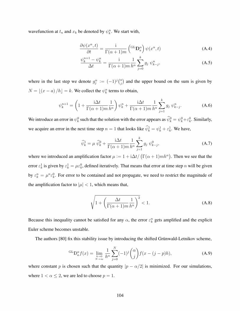
wavefunction at tn and xk be denoted by ψnk . We start with,
∂ψ(xα, t)
∂t=
i
Γ(α + 1)m
(GLDα
a
)ψ(xα, t) (A.4)
ψn+1k − ψnk
∆t=
i
Γ(α + 1)m
1
hα
k∑j=0
gj ψnk−j, (A.5)
where in the last step we denote gαj := (−1)j(αj
)and the upper bound on the sum is given by
N = b(x− a) /hc = k. We collect the ψnk terms to obtain,
ψn+1k =
(1 +
i∆t
Γ(α + 1)m
1
hα
)ψnk +
i∆t
Γ(α + 1)m
1
hα
k∑j=1
gj ψnk−j. (A.6)
We introduce an error in ψ0k such that the solution with the error appears as ψ0
k = ψ0k+ε0k. Similarly,
we acquire an error in the next time step n = 1 that looks like ψ1k = ψ1
k + ε1k. We have,
ψ1k = µ ψ0
k +i∆t
Γ(α + 1)m
1
hα
k∑j=1
gj ψ0k−j, (A.7)
where we introduced an amplification factor µ := 1 + i∆t/(Γ(α + 1)mhα
). Then we see that the
error ε1k is given by ε1k = µε0k, defined iteratively. That means that error at time step n will be given
by εnk = µnε0k. For error to be contained and not propagate, we need to restrict the magnitude of
the amplification factor to |µ| < 1, which means that,
√1 +
(∆t
Γ(α + 1)m
1
hα
)2
< 1. (A.8)
Because this inequality cannot be satisfied for any α, the error εnk gets amplified and the explicit
Euler scheme becomes unstable.
The authors [80] fix this stability issue by introducing the shifted Grunwald-Letnikov scheme,
GLDαaf(x) = lim
h→0N→∞
1
hα
N∑j=0
(−1)j(α
j
)f(x− (j − p)h), (A.9)
where constant p is chosen such that the quantity |p − α/2| is minimized. For our simulations,
where 1 < α ≤ 2, we are led to choose p = 1.
104
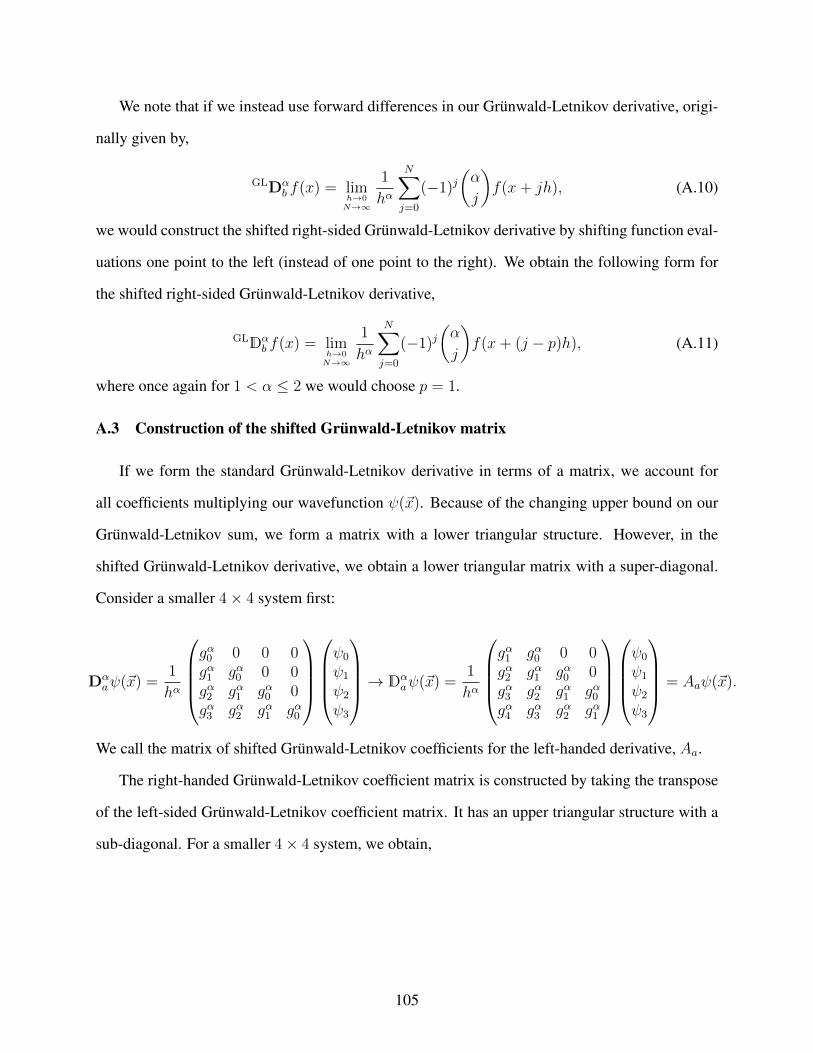
We note that if we instead use forward differences in our Grunwald-Letnikov derivative, origi-
nally given by,
GLDαb f(x) = lim
h→0N→∞
1
hα
N∑j=0
(−1)j(α
j
)f(x+ jh), (A.10)
we would construct the shifted right-sided Grunwald-Letnikov derivative by shifting function eval-
uations one point to the left (instead of one point to the right). We obtain the following form for
the shifted right-sided Grunwald-Letnikov derivative,
GLDαb f(x) = lim
h→0N→∞
1
hα
N∑j=0
(−1)j(α
j
)f(x+ (j − p)h), (A.11)
where once again for 1 < α ≤ 2 we would choose p = 1.
A.3 Construction of the shifted Grunwald-Letnikov matrix
If we form the standard Grunwald-Letnikov derivative in terms of a matrix, we account for
all coefficients multiplying our wavefunction ψ(~x). Because of the changing upper bound on our
Grunwald-Letnikov sum, we form a matrix with a lower triangular structure. However, in the
shifted Grunwald-Letnikov derivative, we obtain a lower triangular matrix with a super-diagonal.
Consider a smaller 4× 4 system first:
Dαaψ(~x) =
1
hα
gα0 0 0 0gα1 gα0 0 0gα2 gα1 gα0 0gα3 gα2 gα1 gα0
ψ0
ψ1
ψ2
ψ3
→ Dαaψ(~x) =
1
hα
gα1 gα0 0 0gα2 gα1 gα0 0gα3 gα2 gα1 gα0gα4 gα3 gα2 gα1
ψ0
ψ1
ψ2
ψ3
= Aaψ(~x).
We call the matrix of shifted Grunwald-Letnikov coefficients for the left-handed derivative, Aa.
The right-handed Grunwald-Letnikov coefficient matrix is constructed by taking the transpose
of the left-sided Grunwald-Letnikov coefficient matrix. It has an upper triangular structure with a
sub-diagonal. For a smaller 4× 4 system, we obtain,
105
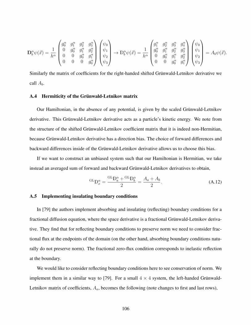
Dαb ψ(~x) =
1
hα
gα0 gα1 gα2 gα30 gα0 gα1 gα20 0 gα0 gα10 0 0 gα0
ψ0
ψ1
ψ2
ψ3
→ Dαb ψ(~x) =
1
hα
gα1 gα2 gα3 gα4gα0 gα1 gα2 gα30 gα0 gα1 gα20 0 gα0 gα1
ψ0
ψ1
ψ2
ψ3
= Abψ(~x).
Similarly the matrix of coefficients for the right-handed shifted Grunwald-Letnikov derivative we
call Ab.
A.4 Hermiticity of the Grunwald-Letnikov matrix
Our Hamiltonian, in the absence of any potential, is given by the scaled Grunwald-Letnikov
derivative. This Grunwald-Letnikov derivative acts as a particle’s kinetic energy. We note from
the structure of the shifted Grunwald-Letnikov coefficient matrix that it is indeed non-Hermitian,
because Grunwald-Letnikov derivative has a direction bias. The choice of forward differences and
backward differences inside of the Grunwald-Letnikov derivative allows us to choose this bias.
If we want to construct an unbiased system such that our Hamiltonian is Hermitian, we take
instead an averaged sum of forward and backward Grunwald-Letnikov derivatives to obtain,
GLDαx =
GLDαa + GLDα
b
2=Aa + Ab
2. (A.12)
A.5 Implementing insulating boundary conditions
In [79] the authors implement absorbing and insulating (reflecting) boundary conditions for a
fractional diffusion equation, where the space derivative is a fractional Grunwald-Letnikov deriva-
tive. They find that for reflecting boundary conditions to preserve norm we need to consider frac-
tional flux at the endpoints of the domain (on the other hand, absorbing boundary conditions natu-
rally do not preserve norm). The fractional zero-flux condition corresponds to inelastic reflection
at the boundary.
We would like to consider reflecting boundary conditions here to see conservation of norm. We
implement them in a similar way to [79]. For a small 4 × 4 system, the left-handed Grunwald-
Letnikov matrix of coefficients, Aa, becomes the following (note changes to first and last rows),
106
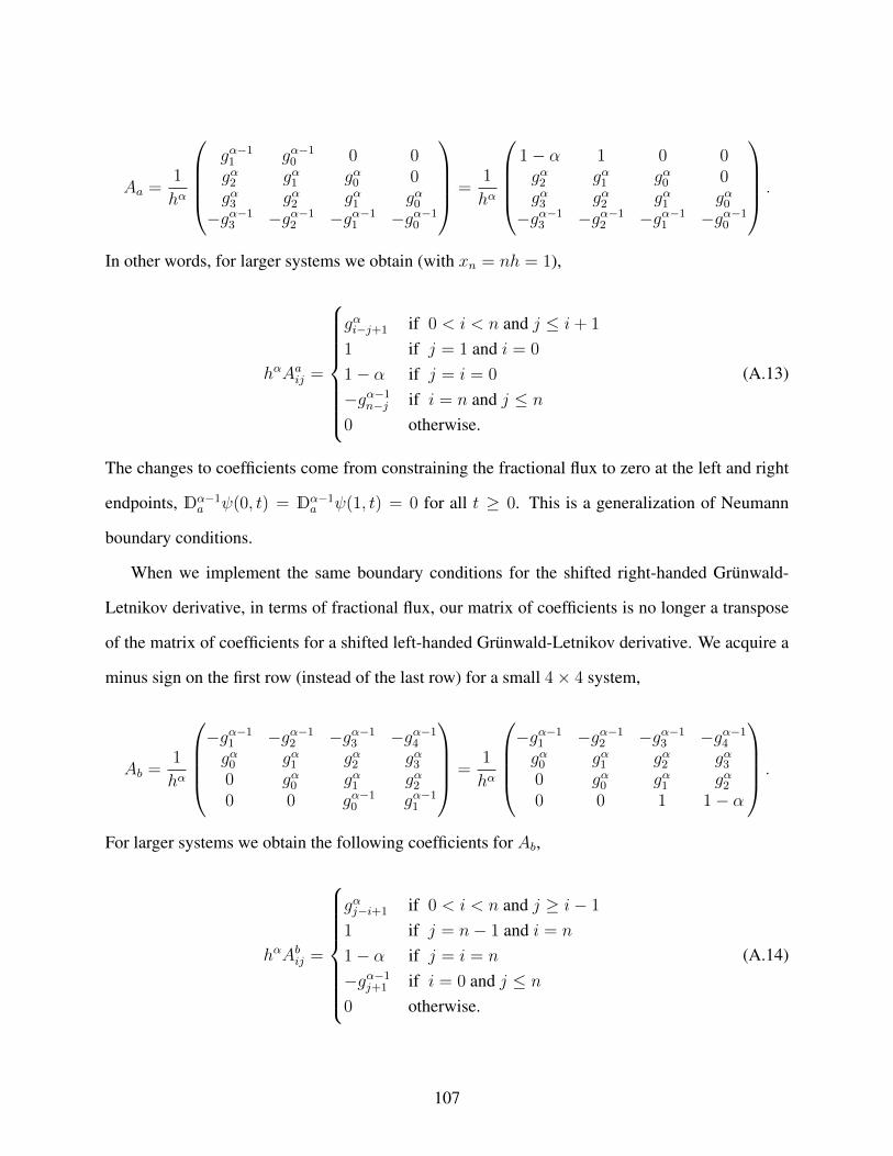
Aa =1
hα
gα−11 gα−10 0 0gα2 gα1 gα0 0gα3 gα2 gα1 gα0−gα−13 −gα−12 −gα−11 −gα−10
=1
hα
1− α 1 0 0gα2 gα1 gα0 0gα3 gα2 gα1 gα0−gα−13 −gα−12 −gα−11 −gα−10
.
In other words, for larger systems we obtain (with xn = nh = 1),
hαAaij =
gαi−j+1 if 0 < i < n and j ≤ i+ 1
1 if j = 1 and i = 0
1− α if j = i = 0
−gα−1n−j if i = n and j ≤ n
0 otherwise.
(A.13)
The changes to coefficients come from constraining the fractional flux to zero at the left and right
endpoints, Dα−1a ψ(0, t) = Dα−1
a ψ(1, t) = 0 for all t ≥ 0. This is a generalization of Neumann
boundary conditions.
When we implement the same boundary conditions for the shifted right-handed Grunwald-
Letnikov derivative, in terms of fractional flux, our matrix of coefficients is no longer a transpose
of the matrix of coefficients for a shifted left-handed Grunwald-Letnikov derivative. We acquire a
minus sign on the first row (instead of the last row) for a small 4× 4 system,
Ab =1
hα
−gα−11 −gα−12 −gα−13 −gα−14
gα0 gα1 gα2 gα30 gα0 gα1 gα20 0 gα−10 gα−11
=1
hα
−gα−11 −gα−12 −gα−13 −gα−14
gα0 gα1 gα2 gα30 gα0 gα1 gα20 0 1 1− α
.
For larger systems we obtain the following coefficients for Ab,
hαAbij =
gαj−i+1 if 0 < i < n and j ≥ i− 1
1 if j = n− 1 and i = n
1− α if j = i = n
−gα−1j+1 if i = 0 and j ≤ n
0 otherwise.
(A.14)
107
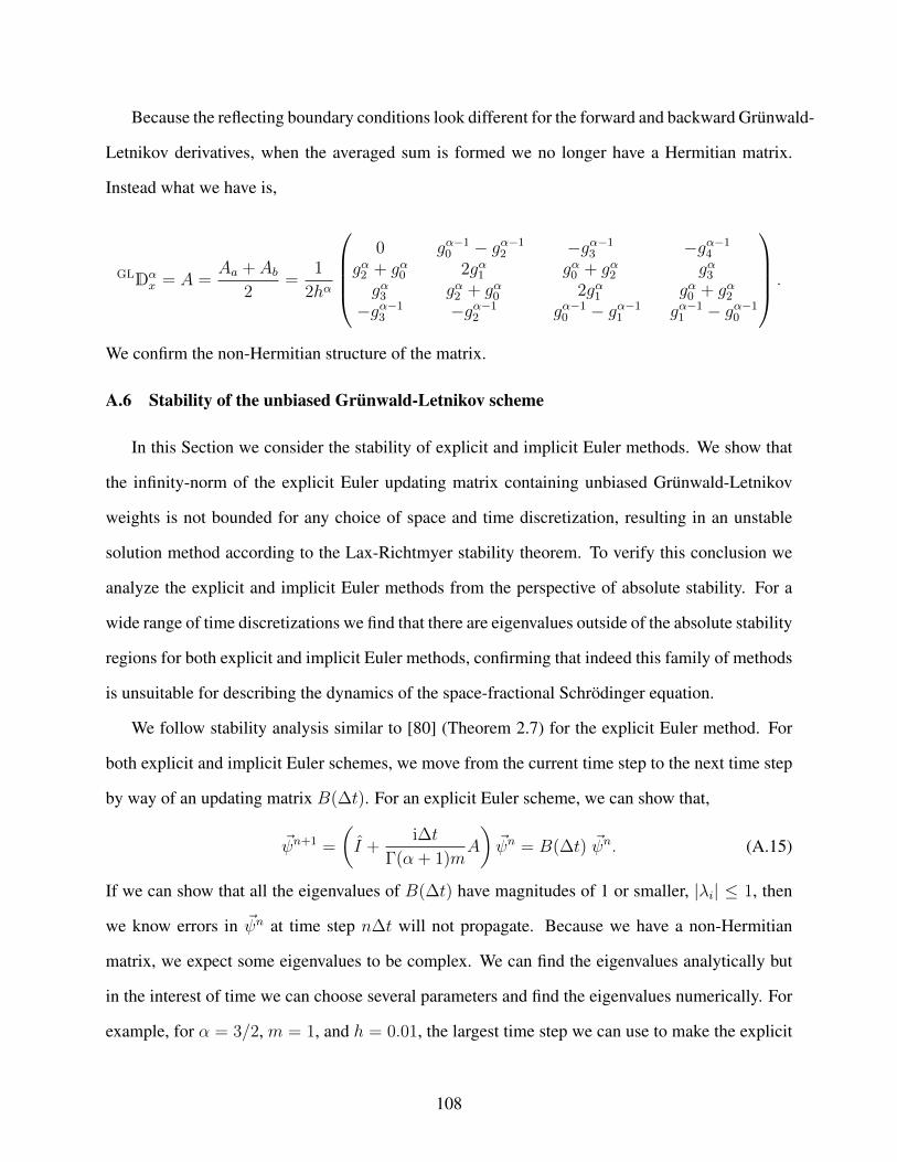
Because the reflecting boundary conditions look different for the forward and backward Grunwald-
Letnikov derivatives, when the averaged sum is formed we no longer have a Hermitian matrix.
Instead what we have is,
GLDαx = A =
Aa + Ab2
=1
2hα
0 gα−10 − gα−12 −gα−13 −gα−14
gα2 + gα0 2gα1 gα0 + gα2 gα3gα3 gα2 + gα0 2gα1 gα0 + gα2−gα−13 −gα−12 gα−10 − gα−11 gα−11 − gα−10
.
We confirm the non-Hermitian structure of the matrix.
A.6 Stability of the unbiased Grunwald-Letnikov scheme
In this Section we consider the stability of explicit and implicit Euler methods. We show that
the infinity-norm of the explicit Euler updating matrix containing unbiased Grunwald-Letnikov
weights is not bounded for any choice of space and time discretization, resulting in an unstable
solution method according to the Lax-Richtmyer stability theorem. To verify this conclusion we
analyze the explicit and implicit Euler methods from the perspective of absolute stability. For a
wide range of time discretizations we find that there are eigenvalues outside of the absolute stability
regions for both explicit and implicit Euler methods, confirming that indeed this family of methods
is unsuitable for describing the dynamics of the space-fractional Schrodinger equation.
We follow stability analysis similar to [80] (Theorem 2.7) for the explicit Euler method. For
both explicit and implicit Euler schemes, we move from the current time step to the next time step
by way of an updating matrix B(∆t). For an explicit Euler scheme, we can show that,
~ψn+1 =
(I +
i∆t
Γ(α + 1)mA
)~ψn = B(∆t) ~ψn. (A.15)
If we can show that all the eigenvalues of B(∆t) have magnitudes of 1 or smaller, |λi| ≤ 1, then
we know errors in ~ψn at time step n∆t will not propagate. Because we have a non-Hermitian
matrix, we expect some eigenvalues to be complex. We can find the eigenvalues analytically but
in the interest of time we can choose several parameters and find the eigenvalues numerically. For
example, for α = 3/2, m = 1, and h = 0.01, the largest time step we can use to make the explicit
108
Euler method stable to 14 decimal places is ∆t = 1e –11. This is clearly an impractical scheme.
Let’s ask why that happens. We make use of Lax-Richtmyer stability, defined as in [81].
• Definition (Lax-Richtmyer stability)
Consider a linear matrix system given by
un+1 = B(∆t)un + bn(∆t) where B = B(∆t) ∈ Rm×m, u, bn(∆t) ∈ Rm, (A.16)
where ∆x = 1/(m + 1) because our system is already discretized. Then this linear method is
Lax-Richtmyer stable if, for each time T , there is a constant CT > 0 such that∥∥B(∆t)n∥∥ ≤ CT (A.17)
for all ∆t > 0 and integers n for which n∆t ≤ T .
We can choose any norm to satisfy the inequality, and to make things easier on us we choose the
infinity-norm ||·||∞ (in general there exists an equivalence statement relating one norm to another).
The infinity-norm corresponds to the maximum of the sum of all absolute-valued elements in each
row. Let’s start by finding the infinity-norm for our matrix A.
The matrix A contains positive real values except when i = j (excluding i = 0, n rows), which
correspond to Aii = gα1 = −α. To take the absolute value of each element in a row we have to
replace gα1 with −gα1 , and then we compute the sum. Empirically we see that elements of A are
largest when i = i0 = b(n+ 1) /2c.
We can show then that, depending on whether n is even or odd, the infinity-norm of A is given
by,
hα‖A‖∞ =
(n+2)/2∑i=0i 6=1
gαi − gα1 when n is even, (A.18)
hα‖A‖∞ =
(n+1)/2∑i=0i 6=1
gαi − gα1 +gαn+3
2
2when n is odd, (A.19)
109
where we account for the fact that gα1 is negative. Our fractional Schrodinger system can be writ-
ten down as Eq. (A.15), where B(∆t) matches the form of the linear matrix system in the Lax-
Richtmyer stability definition.
We make use of the following three properties for the infinity-norm. With A,B ∈ Rn×n and
α ∈ C, we have,
1. ‖AB‖∞ ≤‖A‖∞ ‖B‖∞ (A.20)
2. ‖A+B‖∞ ≤‖A‖∞ + ‖B‖∞ (A.21)
3. ‖αA‖∞ = |α| ‖A‖∞ . (A.22)
The first is known as the submultiplicative property, and the second is the triangle inequality. We
would like to compute powers of B(∆t) to find∥∥B(∆t)`
∥∥∞. We consider even n for simplicity.
First, by the submultiplicative property we expand the infinity-norm of a matrix into a product of
infinity-norms of matrices,
∥∥∥B(∆t)`∥∥∥∞
=
∥∥∥∥∥(I +
i∆t
Γ(α + 1)mA
)`∥∥∥∥∥∞
(A.23)
∥∥∥B(∆t)`∥∥∥∞≤∥∥B(∆t)
∥∥∞
∥∥B(∆t)∥∥∞ · · ·
∥∥B(∆t)∥∥∞︸ ︷︷ ︸
` times
=
∥∥∥∥∥(I +
i∆t
Γ(α + 1)mA
)∥∥∥∥∥`
∞
(A.24)
∥∥∥∥∥(I +
i∆t
Γ(α + 1)mA
)∥∥∥∥∥`
∞
≤(
1 +∆t
Γ(α + 1)m‖A‖∞
)`(A.25)
∥∥∥B(∆t)`∥∥∥∞≤
1 +∆t
hα1
Γ(α + 1)m
(n+2)/2∑i=0i 6=1
gαi − gα1
`
. (A.26)
In Eq. (A.25) we used the triangle inequality. We define the ratio k = ∆t/hα and the upper bound
on the sum N = (n+ 2) /2. For the explicit Euler scheme to be Lax-Richtmyer stable we hope to
find the expression in Eq. (A.26) bounded by a constant L for all ∆t > 0. We can further simplify
110
the expression by explicitly summing up the binomial coefficients to obtain,
∥∥∥B(∆t)`∥∥∥∞≤
1 +k
Γ(α + 1)m
[2α + (−1)N
(α− 1
N
)]`
(A.27)
∥∥∥B(∆t)`∥∥∥∞≤(
1 +k
Γ(α + 1)m
(2α + gα−1N
))`. (A.28)
If the quantity in the parentheses is equal to or less than 1, its powers will be equal to or less than
1. However, we can see that if ∆t and h are on the same order of magnitude then k ≥ 1 and
serves to amplify the quantity in the square brackets. Only when we take the limit ∆t → 0 does
the amplification factor tend to 1. This is also what we found with the eigenvalue analysis for the
explicit Euler scheme.
Another way to look at stability is to find the eigenvalues of the initial matrix on the right-
hand side (before any scheme is applied to represent the time derivative), which for us is A :=
iA/(Γ(α + 1)m
). Every method that approximates the time derivative on the left-hand side comes
with its own absolute stability region. We consider the absolute stability definition for a linear
system [81]:
• Definition (Absolute stability)
Consider a linear matrix system given by{∂t~u(t) = A ~u(t) where A ∈ Rm×m, ~u ∈ Rm
~u(t0) = ~u0.(A.29)
Then a finite difference method is stable for this linear system if zi = λi∆t is in the absolute
stability region of that method for all eigenvalues λi of A, provided A is diagonalizable.
For the implicit Euler scheme, this stability region is anywhere in the complex plane that is
outside of a circle of unit radius centered at z = 1, |z − 1| ≥ 1, where z = λ∆t. (Eigenvalues are
assumed in general to be complex). We find that at least one of the eigenvalues of A for the same
parameters of α,m, and h as for the explicit Euler method is contained in the forbidden region
111
|z − 1| ≤ 1 for a range of reasonable ∆t. Indeed, as ∆t is decreased, more eigenvalues fall into
the forbidden region. This tells us that the implicit Euler scheme is unconditionally unstable when
applied to the fractional Schrodinger equation.
A.7 Note on absorbing boundary conditions
Absorbing (Dirichlet) boundary conditions fix the wavefunction value at the boundary, for
example, when we consider the infinite square well potential on a unit interval we require that,
ψ(0, t) = ψ(1, t) = 0 for all t ≥ 0. (A.30)
Unlike box boundary conditions commonly used in physics, absorbing boundary conditions do not
conserve norm [79]. Instead of balancing out the accumulating norm at the boundary in such a way
that the wavefunction is made zero, absorbing boundary conditions set the non-zero Grunwald-
Letnikov boundary coefficients responsible for norm accumulation to zero. This in effect models
infinite domain and the norm of the wavefunction decreases. To ensure zero boundary conditions
we set Grunwald-Letnikov matrix elements to 0 in the first and last rows, obtaining,
hαAaij =
{gαi−j+1 if 0 < i < n and j ≤ i+ 1
0 otherwise(A.31)
hαAbij =
{gαj−i+1 if 0 < i < n and j ≥ i− 1
0 otherwise.(A.32)
We note that A = (Aa + Ab) /2 is now symmetric and the Hamiltonian Hermitian. However,
the infinity-norm of A is not affected since the zero rows do not alter the maximum sum of row
elements, and thus explicit and implicit Euler methods considered in Section A.6 are still unstable.
A.8 Conclusions
In this numerical exploration we considered the Grunwald-Letnikov fractional space derivative
for the fractional Schrodinger equation. We found in Section A.2 that the standard Grunwald-
Letnikov scheme is unconditionally unstable, and that to make it stable we have to shift function
112
evaluations one step to the right or left, depending on the original bias of the Grunwald-Letnikov
matrix. Shifted, one-sided Grunwald-Letnikov derivatives have a direction bias which leads to a
non-Hermitian Hamiltonian. We instead took an averaged sum of forward and backward shifted
Grunwald-Letnikov derivatives to achieve Hermiticity, however, when insulating boundary condi-
tions were realized in terms of a zero fractional flux on the edges of the domain, the Grunwald-
Letnikov matrix lost its Hermitian structure.
Finally, in Section A.6 we showed that the averaged Grunwald-Letnikov matrix wasn’t Lax-
Richtmyer stable for the explicit Euler method. We checked absolute stability and Lax-Richtmyer
stability in three different contexts for the averaged Grunwald-Letnikov derivative with no direction
bias. Because both explicit and implicit Euler methods were unstable when applied to the fractional
Schrodinger equation, a more refined numerical method is likely to fail.
113