Reallocation and Technology:Evidence from the U.S. Steel Industry ∗

Allan Collard-Wexler and Jan De LoeckerNYU and NBER, and Princeton University, NBER and CEPR

December 19, 2013

Abstract

We measure the impact of a drastic new technology for producing steel – the minimill – onthe aggregate productivity of U.S. steel producers, using unique plant-level data between 1963 and2002. We find that the sharp increase in the industry’s productivity is linked to this new technologythrough two distinct mechanisms. First, minimills displaced the older technology, called verticallyintegrated production, and this reallocation of output was responsible for a third of the increasein the industry’s productivity. Second, increased competition, due to the expansion of minimills,drove a substantial reallocation process within the group of vertically integrated producers, drivinga resurgence in their productivity and, consequently, the productivity of the industry as a whole.

Keywords: Productivity; Technology; Competition; Reallocation.

∗This project was funded by the Center for Economic Policy Studies (CEPS) at Princeton University and the Center forGlobal Economy and Business (CGEB) at New York University. We would like to thank Jun Wen for excellent researchassistance, and Jonathan Fisher for conversations and help with Census Data. We would like to thank the co-Editor (LuigiPistaferri) and three anonymous referees for excellent comments and suggestions. Furthermore, we thank Nick Bloom,Rob Clark, Liran Einav, Ariel Pakes, Kathryn Shaw, Chad Syverson, Raluca Dragusanu, and seminar participants at manyinstitutions. This paper uses restricted data that were analyzed at the U.S. Census Bureau Research Data Center in New YorkCity. Any opinions and conclusions expressed herein are those of the authors and do not necessarily represent the views of theU.S. Census Bureau. All results have been reviewed to ensure that no confidential information is disclosed. Contact details:Allan Collard-Wexler, wexler@nyu.edu; and Jan De Loecker, jdeloeck@princeton.edu. The usual caveat applies.

1

1 Introduction

Identifying the sources of productivity growth of firms, industries, and countries, has been a central

question for economic research. There remain, however, many empirical obstacles to credibly iden-

tifying the underlying sources of productivity growth. First, the measurement of productivity at the

producer level typically requires an estimate of the production function and, therefore, has to confront

both the endogeneity of inputs and unobserved prices for inputs and outputs. Second, it is difficult

to observe potential explanatory variables at the producer level, such as technology, competition, and

management practices.1 Finally, in order to establish causality, exogenous shifters of such variables are

required in order to trace out their effects on productivity.

A recent literature has emphasized the distinction between the productivity effects that occur at

the producer level, and those realized by moving resources between producers – i.e., the reallocation

mechanism. Although it is now well established, at both a theoretical and empirical level, that the

reallocation of resources across producers is important in explaining aggregate outcomes, it has been

very hard to identify the exact mechanisms behind it.2 In this paper, we focus on the role of technology

and the associated changes in competition in driving the reallocation process underlying aggregate

productivity growth.

We examine one particular industry, the U.S. steel sector, for which we have detailed producer-level

production and price data. Our setting is well suited to measuring the role of technological change,

since we directly observe the exogenous arrival of a new production process – the minimill – at the

plant level. In addition, we observe detailed output and input data, including physical measures of

inputs and outputs, as well as standard revenue and expenditure data, to obtain measures of productivity

and market power. These inputs and outputs are remarkably unchanging over a 40-year period, and the

steel products shipped in the 1960s are very similar to those shipped in 2002. Thus, productivity growth

in steel is almost uniquely driven by process innovation, rather than through the introduction of new

goods. Observing a panel of steel producers over a 40-year period, 1963-2002, allows us to study the

long-run implications of increased competition, such as the slow entry and exit process.

The U.S. steel industry shed about 75 percent of its workforce between 1962 and 2005, or about

400,000 employees. This dramatic fall in employment has far-reaching economic and social implica-

tions. For example, between 1950 and 2000, Pittsburgh – which used to be the center of the U.S. Steel

Industry – dropped from the tenth-largest city in the United States to the 52nd largest.

While employment in the steel sector fell by a factor of five, shipments of steel products in 20051See Syverson (2011) for an excellent overview of the various potential determinants of productivity at both the producer

and the industry level. Two prominent studies on the triggers of productivity growth are Schmitz (2005) and Olley andPakes (1996), who study the role of two such triggers: import competition in the iron ore market and deregulation in thetelecommunications market. Hortacsu and Syverson (2004), Bloom et al. (2013), and Jarmin et al. (2009) show that factorssuch as vertical integration, management, and large retail chains lead to systematic differences in productivity between plantsand consequently, have implications for aggregate industry performance.

2For instance, Melitz (2003), shows how trade liberalization impacts aggregate productivity through a reallocation towardsmore-productive firms, while Foster et al. (2001) and Bartelsman et al. (2009) document the role of reallocation empirically.

2

reached the level of the early 1960s. Thus, output per worker grew by a factor of five, while total factor

productivity (TFP) increased by 38 percent. This makes the steel sector one of the fastest growing

of the manufacturing industries over the last three decades, behind only the computer software and

equipment industries. We highlight the special features of the U.S. steel industry in Table 1, where we

report its change in output, input use, TFP and prices over the period 1972-2002 and compare it to the

mean and median manufacturing sector’s experience.

Table 1 points out the unique feature of the steel industry: The period of impressive productivity

growth – 28 percent compared to the median of three percent – occurred while the sector contracted by

35 percent. The starkest difference is the drop in employment of 80 percent compared to a decline of

five percent for the average sector.

We find that the main reason for the rapid productivity growth and the associated decline in em-

ployment is neither a steady drop in steel consumption nor the emergence of globalization. Nor is it a

displacement of production away from the midwest. The increase in productivity can be directly linked

to the introduction of a new production technology, the steel minimill. The minimill displaced the older

technology, called vertically integrated production, and this reallocation of output was responsible for

about a third of the increase in the industry’s total factor productivity. In addition, minimills’ produc-

tivity steadily increased. We can directly attribute almost half of the aggregate productivity growth in

steel to the entry of this new technology.

However, the older technology was not entirely displaced. Instead, vertically integrated producers

experienced a dramatic resurgence of productivity and, by 2002, were on average, as productive as min-

imills. This resurgence was not driven by improvements at integrated plants. Rather, less-productive

vertically integrated plants were driven out of the industry, and output was reallocated to more-efficient

producers. We see exit of vertically integrated producers in precisely the product segments where they

competed head-to-head with minimills.

When we evaluate the impact of a drastic technological change on aggregate productivity growth,

we also control for other potential drivers of productivity growth, including international competition,

geography, and firm-level factors such as organization and management. We also show that markups in

this industry fell by 50 percent over the last 40-years, which is not surprising if we look at the output

and input price changes in Table 1. This increase in productivity, and fall in markups, jointly lead to a

predicted increase in consumer surplus of between nine and 11 billion dollars per year.

In addition to identifying the exact mechanisms underlying productivity growth, which are of in-

terest to a growing literature on reallocation and productivity dispersion, the steel industry is also

important in and of itself. Even today, it is one of the largest sectors in U.S. manufacturing: In 2007,

steel plants had shipments of over 100 billion dollars, of which half was value added. Therefore,

understanding the sources of productivity growth in this industry is of independent interest.

The remainder of the paper is organized as follows. Section 2 describes the data. In Section 3, we

present five key facts that help guide the empirical analysis, which we take up in Sections 4 and 5. We

discuss alternative specifications and robustness in Section 6 and conclude in Section 7.

3

2 Data

We study the production of steel: plants engaged in the production of either carbon or alloy steels. We

rely on detailed Census micro data to investigate the mechanisms underlying the impressive productiv-

ity growth in the U.S. steel sector. Our analysis is based on plant-level production data of U.S. steel

mills from 1963 to 2002.

We use data provided by the Center for Economics Studies at the United States Census Bureau.

Our primary sources are the Census of Manufacturers (CMF), the Annual Survey of Manufacturers

(ASM), and the Longitudinal Business Database (LBD). We select plants engaged in the production of

steel, coded in either NAICS (North American Industrial Classification) code 33111, or SIC (Standard

Industrial Classification) code 3312. The CMF is sent to all steel mills every five years, while the ASM

is sent to about 50 percent of plants in non-Census years. However, the ASM samples all plants with

over 250 employees and, encompasses over 90 percent of the steel sector’s output.

In addition, we collect data on the products produced at each plant using the product trailer to the

CMF and the ASM, and we collect the materials consumed by these plants from the material trailer to

the CMF.

We rely on our detailed micro data to divide steel mills into two technologies: Minimills (MM,

hereafter) and Vertically Integrated (VI, hereafter) Producers. VI production takes place in two steps.

The first stage takes place in a blast furnace, which combines coke, iron ore, and limestone to produce

pig iron and slag. In the second stage, the pig iron, along with oxygen and fuel, is then used in a basic

oxygen furnace (BOF) to produce steel.3 The steel products produced in either MM or VI plants are

shaped into sheets, bars, wire, and tube in rolling mills. These rolling mills are frequently collocated

with steel mills, but can also be freestanding units.

In contrast, MMs are identified primarily by the use of an electric arc furnace (EAF) to melt down

a combination of scrap steel and direct reduced iron.4 Because these mills have a far smaller efficient

scale, they are, on average, an order of magnitude smaller than vertically integrated producers. His-

torically, EAFs were used to produce lower-quality steel, such as that used to make steel bars, while

virtually all steel sheet (needing higher-quality steel) was produced in BOFs. However, since the mid-

1980s, innovation in the EAFs has enabled them to produce certain types of sheet products, as well.5

We classify plants as minimills, vertically integrated plants, and rolling mills using their responses3There were a few open-hearth furnaces in operation during the sample period. However, as of the late 1960s, open-hearth

plants accounted for only a very small portion of output, and the last open-hearth plant closed in 1991. See Oster (1982) formore on the diffusion of BOF mills.

4The median scrap vintage is quite old, as one would expect, with items such as rails, construction rebar, and other whitegoods accounting for a large share of scrap. Moreover, in the United States, there is an abundant supply of scrap. Indeed,the largest steel export from the United States, by quite a margin, is steel scrap destined for minimills in China and Japan. Itis also possible to produce steel in a minimill without scrap: Direct Reduced Iron (DRI) is a substitute for scrap. Typically,the prices for DRI have been higher than for scrap, but minimills could also exist in a world without vertically integratedproduction of steel. There was a worry in the industry during the 1970s that scrap would become scarce, and, thus, somedirect reduced iron facilities were built. See Chapter 5, page 95, in Barnett and Crandall (1986) for a discussion.

5EAFs have a long history in steel making. However, before the 1960s, they primarily produced specialty steels.

4

to a specific questionnaire on steel mills attached to the 1992, 1997, and 2002 CMF. For prior years,

we use the material and products produced by each plant to identify MM and VI plants. More detail

on the classification of plants can be found in Appendix A. Table B.1 shows summary statistics for the

sample of MM and VI plants. The average VI plant had shipments of 647 million dollars, of which 47

percent is value added, while the average MM plant shipped 153 million dollars, of which 44 percent

is value added, where all dollar amounts are in 1997 $.

3 Key Facts in the U.S. Steel Sector 1963-2002

In this section, we briefly go over some key facts of the U.S. steel sector. These facts will be important

to keep in mind when we analyze the sources of productivity growth.

3.1 Stagnant Shipments, Rising Productivity

From Table 1, we know that the productivity growth in the U.S. steel sector was one of the fastest in

manufacturing. To better understand this period of impressive productivity growth, we plot total output

next to labor and capital use in Figure 1. An important observation is that the period of productivity

growth came about while the industry as a whole contracted severely: Steel producers sold about 60

billion dollars in 1960 and, reached 100 billion dollars in shipments by the early 1970s. A decade later,

only 40 billion dollars of production was shipped, or, put differently, the sector’s shipments decreased

by more than half.

Total employment, on the other hand, decreased consistently, even during the recovery of output in

the late 1980s and throughout the 1990s. The employment panel of Figure 1 shows that total employ-

ment fell from 500,000 to 100,000 employees – one of the sharpest drops in employment experienced

by any sector in the U.S. economy. By 2000, the steel industry employed a fifth of the number of work-

ers that it had in 1960, while production of steel went from 130 million tons in 1960 to 110 million

tons in 2000. This implies that output per worker increased from 260 to 1100 tons.6 Total material

use tracks output quite closely, while labor and capital fell continuously over the entire period, which

suggests that TFP had to increase to offset the sharp drop in labor and capital.7

3.2 A New Production Technology: Minimills

The entry of minimills in steel production constituted a drastic change in the actual production process

of steel products. A natural question to ask is whether MM are any different than the traditional VI steel

producers. We rely on a descriptive OLS regression, where we regress various plant characteristics on6Shipments of steel in tons are collected from various Iron and Steel Institute Annual Statistical Reports (American Iron

and Steel Institute, 2010).7For this aggregate analysis, we rely on the NBER’s five-factor TFP estimate. See Bartelsman et al. (2000) for more

detail.

5

an indicator variable for whether a plant is a vertically integrated producer. We consider a log specifi-

cation such that the coefficient on the technology dummy directly measures the percentage premium of

VI plants.

Table B.2 lists the set of estimated coefficients, and confirms that vertically integrated producers

are, on average, four times bigger, as measured by the large coefficients on shipments, value added, and

inputs. For example, VI plants, on average, ship 144 percent more than MMs. Moreover, VI producers

generate about 20 percent more shipments per worker, which suggests that they are more productive.

However, when we combine the coefficients on all three inputs (labor, materials and capital) with the

shipment premium, we see that total factor productivity (TFP) of MM is at least as high as that of VI

producers. We conduct a more precise comparison of TFP across technologies in Section 4.

In addition to the average premium over the entire sample, we report time-specific coefficients.

Across all the various characteristics, the VI coefficient falls over time. Most notably, shipments per

worker were 23-percent higher for VI plants in 1963, but by 2002, there was no significant difference

between the two technologies in terms of labor productivity. This pattern suggests that, over time, VI

and MM producers became more alike, although VI producers still produce on a larger scale.

The coefficients on wages of six percent, shown in the last row of Table B.2, confirms the well-

known fact that VI producers, on average, pay higher wages. This is likely due to the impact of union-

ization – minimill workers typically being non-unionized.8 It is interesting to note that this average

difference in wages of six percent would only translate into a difference in costs of only 1.2 percent

given the input share of labor for steel producers.

We also find large differences in standard measures of performance, such as profit margins, defined

as sales minus cost of materials and salaries over sales, and the rate of return on capital, defined as sales

minus cost of materials and salaries over capital. Table B.4 considers quantile regressions of either the

profit margin or the rate of return on capital on an indicator for whether or not a plant is vertically

integrated, along with a full set of year fixed-effects. We find that minimills have a rate of return on

capital that is 18-percent higher than for vertically integrated plants. In addition, minimills have a

profit margin that is four-percent higher than that of vertically integrated plants. Minimills are less

capital-intensive than vertically integrated plants, and this explains some of the discrepancy between

these measures of profitability.

An important difference between MM and VI producers is the set of products they manufacture.

Figure 2 shows that in 1997, MMs accounted for 59 percent and 68 percent of shipments of steel

ingots and hot-rolled bar respectively, but only 15 percent and 14 percent of hot and cold rolled sheet.

MMs typically produce lower-quality steel products, which are generally thicker products, while VI

plants produce higher-quality products, which are usually sheet products. However, the product mix

accounted for by MMs changed dramatically over the last 40 years. Figure 2 shows that, in 1977, MMs

produced 27 percent of steel ingots and 24 percent of hot-rolled bar. Between 1977 and 1982, MMs8See Hoerr (1988) – and in particular, page 16 – for evidence of the role of unionization on wages for VI and MM

producers. We discuss the role of unions in more detail in Section 4.2

6

increased their share of both of these products to 40 percent, and by 2002, they produced 81 percent of

hot-rolled bar. As stated above, in 1997, only 15 percent and 14 percent of hot and cold rolled sheet

were produced by MMs.9 Thus, the market share of MMs in the higher-quality product segments, sheet

products, was rather stable up to 1997, after which their market shares increased substantially.

3.3 A Stable Product Mix over Time

We list the product mix of the steel industry in Table B.3. We break down steel into various products:

a) hot-rolled steel sheet (HRS); b) hot-rolled bar (HRB); c) cold-rolled sheet (CRS); d) ingots and

shapes; e) pipe and tube (P&T); f) Wire g) cold-finished bars (CFB); and h) coke oven and blast

furnace products (Blast). Over 40 years, the product mix for steel has barely changed. Hot-rolled sheet

accounted for 23 percent of shipments in 1963 and 31 percent in 2002, and hot-rolled bar accounted

for 23 percent of shipments in 1963 and 22 percent in 2002.

The fact that the steel industry’s products have been unchanged is essential for our identification of

productivity growth, as the industry’s production process has changed far more than its products.

3.4 Heterogeneous Price Trends Across Products

While steel producers’ product mix has been relatively unchanged from 1963 to today, the prices for

these products have dropped considerably, which is not surprising given the large increases in TFP in

the industry. Panel A of Figure 3 presents the price indices for the four main products – hot and cold

rolled sheet, hot rolled bar and steel ingots – which, taken together, represent 80 percent of shipments

in 1997.10

The same panel shows that the prices of all steel products followed a very similar, and gradually

increasing, pattern up to 1980. But from 1982 to 2000, we see 50-percent drop in the real price of

steel. This implies that, while shipments of steel in dollars dropped since 1980, the quantity shipped

has gradually increased since the mid-1980s (see Panel 1 of Figure 1).11

In addition, when we decompose these price trends further, we find that the prices of hot-rolled

bars and steel ingots have fallen faster than the prices of hot and cold rolled sheet. While sheet steel

is produced primarily by VI producers, prices for bar and ingot products fell by ten percent more than

those for sheet products in 1982-1984. This occurred precisely at the point at which MMs saw an

increase in their market share of bar and ingot products.

Turning to prices for inputs, we construct an intermediate input price index Pnt for each intermedi-

ate input n, where n = Fuels, Electricity, Coal for Coke, Iron Ore, and Scrap Steel, using either the

NBER fuel price deflator, or reported quantities and costs in the material trailer to the CMF (which9Giarratani et al. (2007) discuss the entry of Minimills into the production of sheet products around 1990.

10We have taken care to deflate these price indices by the GDP deflator to show price trends for steel relative to the rest ofthe economy.

11Annual reports of the American Iron and Steel Institute (2010), where total tons of steel are recorded annually, indicatethat quantity produced increased by about 30 percent between 1982 and 2002.

7

allow us to back out prices). We construct a plant-specific input price index (PMit ) using a weighted

average of these intermediate input-specific prices, Pnt, where the weights are the share of an interme-

diate n in total intermediate input use.12

We present the time series pattern of our constructed input price index in Panel B of Figure 3. We

compare the publicly available NBER Material Price Index (NBER MPI) with our constructed input

price index. We compute the mean of the latter by technology and find that the NBER MPI follows our

price index closely. However, the aggregate input price index hides the heterogeneity in input prices,

especially during the energy price spike in the late 1970s and early 1980s. While input prices were

very similar around 1972, by 1982, integrated producers faced almost 20-percent-higher input prices,

primarily because they purchased more energy-intensive inputs.

Therefore, in order to correctly identify the productivity effect of the arrival of the minimills, and

their associated increased competition, it will be imperative to control for price differences, for both

inputs and outputs, across plants and time.

3.5 Simultaneous Entry and Exit

From Figure 1, we know that the number of plants increased over time. In Table 2, we go a step further,

showing both the number of MM and VI plants that entered or exited, as well as the market share these

plants represent. There was marked entry of new plants in the early 1980s, a period during which the

industry as a whole severely contracted.

The market share of plants entering from 1982 to 1992 was 20 percent, versus five percent in the

previous two decades, while the market share of exiters was 18 percent during this period. Most entry

in this period was due to minimills, and most exit was from vertically integrated producers.13 From

these entry and exit statistics, we expect an important role for entry and exit in explaining productivity

growth.

4 Drivers of productivity growth

The previous section highlighted the difference in performance between MM and VI producers, and

suggested a large potential role for reallocation across these technologies in explaining productivity

growth. This paper is concerned with studying the productivity differences in detail and verifying

the extent to which the entry of minimills contributed to the stark aggregate productivity growth in

the industry. We proceed in two steps. First, we present our empirical framework used to estimate

the production function and establish the productivity premium of minimills. Second, we verify the

robustness of this premium by considering alternative drivers of productivity growth.12Appendix C describes the construction of the input price index in detail.13This phenomenon, the speeding up of exit and entry during a downturn, has been documented by Bresnahan and Raff

(1991) for the motor vehicles industry during the Great Depression.

8

4.1 Productivity Differences Across Technology

Denote each technology – either MM or VI – as ψ ∈ V I,MM.14 A plant i at time t can produce

output Qijt of a given product j, using a technology ψ specific production technology:

Qijt = Fψ,t(Lijt,Mijt,Kijt) exp(ωit). (1)

Our notation highlights that VI and MM producers rely on different technologies, which we allow

to vary over time. As is common in the literature, productivity ωit is modeled as a Hicks-neutral term.

Moreover, we assume that productivity is plant-specific.

4.1.1 Measurement

Recovering productivity using revenue and expenditure data requires that we correct for potential price

variation across plants and time, for both output and inputs. Below, we describe our procedure briefly,

and Appendix C provides more details.

In order to recover productivity, ωit, using product-level revenue data for each plant, we assume that

each product j is homogeneous, and we construct a plant-specific output price (Pit) using product-level

BLS price data and then match that in with our production data.15

The bulk of quality variation operates across across product codes, particularly when it comes to

comparing bar products to sheet products – perhaps the most obvious quality metric being how thick

the steel product is, which determines the value for downstream users such as car producers and the

construction industry. Our measures of productivity are designed to control for quality differences that

materialize through price differences and allow for the comparison of plant-level productivity across

producers of different product mixes. Of course, to the extent that there are quality differences across

plants within our narrowly defined products – for example, Hot Rolled Bars broken into low-quality

rebar used for reinforcing concrete versus higher-quality structural steel used to make frames for build-

ings – our measure of productivity will pick up these differences in quality as differences in output.16

The working assumption is, thus, that the main quality differences exist among the nine product codes,

and that the variation within products across plants comes from the cost side – i.e., through productivity

differences.

We follow the literature and consider a Cobb-Douglas specification by type, which gives rise to the14In the steel industry, a plant cannot switch technology, such as a VI plant becoming a MM. This is in contrast to the

a setting of technology adoption, such as Van Biesebroeck (2003)’s empirical analysis of technology adoption in U.S. carmanufacturing.

15We constructed nine product categories, which correspond to 7-digit NAICS codes, which are the most detailed plantlevel production statistics we have access to at Census.

16This is a standard problem in the literature, and with the exception of a few papers, such as De Loecker (2011);De Loecker et al. (2012), the norm is not to have any control for quality, let alone within a narrowly defined product cat-egory.

9

following expression for product-level sales by plant (for each type17):

Rijt = LβlijtMβmijt K

βkijt exp(ωit)Pjt. (2)

We are interested in recovering a measure of productivity at the plant level, and, therefore, aggregate

up to plant-level sales. However, a common restriction in these type of data is that we do not directly

observe the input use by product (see Foster et al. (2008)). We allocate inputs across products using

product-specific sales shares, sRijt =RijtRit

, such that Xijt ≡ sRijtXit with X = L,M,K.18 After

aggregating (2) to the plant level, we obtain19:

Rit∑j s

RijtPjt

= LβlitMβmit Kβk

it exp(ωit). (3)

Although the focus in the literature has been mainly on the heterogeneity of output prices, input

price variation potentially plagues the measurement of productivity, as well. The data on intermediate

input use, Mit, are potentially the most contaminated by input price variation, both in the time-series

and in the cross-section, particularly between MM and VI plants. The two technologies use vastly

different intermediate inputs or use inputs at very different intensities, and, therefore, we expect the

relevant input price to vary substantially across plants of different technologies.20

We construct our input price deflators in a similar way as the output price deflator. First, we need to

distinguish between our three main input categories: labor, intermediate inputs and capital. We directly

observe labor Lit: hours worked at the plant-level. For capital, we rely on the NBER capital deflator

(PKt ) to correct the capital stock series. For materials, we use our plant-level input price deflator PMit .

We estimate the production function using our constructed output and input price deflators, by type,

using:

qit = βllit + βmmit + βkkit + ωit + εit, (4)

where lower cases indicate logs of deflated variables when appropriate.21 We allow for unanticipated

shocks to production and measurement error in output and prices, as captured by εit.22 In the next

subsection, we discuss the estimation and identification of equation (4).17We drop the type subscript ψ and, unless stated otherwise, consider technology-specific production functions.18As discussed in detail in Appendix C, this implies that we implicitly restrict markups to be common across products

within a plant. We are not interested in explaining within-plant markup differences across products, but mainly aim torecover measures of plant-level productivity that are not contaminated by price variation across plants and time.

19Formally, this restricts the attention to constant returns to scale. First, we find strong evidence for constant returns toscale in our data. Second, our approach would only be modified by the inclusion of an additional term

∑j(s

Rijt)

γPjt in theestimating equation, with γ = βl + βm + βk.

20See Appendix C.2.2 for more detail on this point.21E.g., qit = ln

(Rit∑

j sijtPjt

)and mit = ln

(∑n

MEintPnt

).

22Formally, the inclusion of εit is compatible with the existence of measurement error and unanticipated shocks in bothrevenue and price data. E.g., we observe revenue in the data and it relates to a firm’s measure as follows: Rit = R∗it exp(εit).Thus, the error term εit captures, potentially, multiple iid error terms. The distinction is not important for our analysis.

10

4.1.2 Estimation of production functions

We take equation (4) to the data and rely on a plant’s optimal investment to control for unobserved

productivity shocks. We estimate the production function rather than impute the production function

coefficients from first-order conditions (FOC). This FOC approach infers production function coeffi-

cients from input revenue shares, where the coefficient on labor, for example, is simply given by the

wage bill over sales. This approach requires that all inputs are fully flexible, which seems implausible

in the steel industry given the irreversibility of capital investments and union labor contracts. As well,

both output and input markets must be perfectly competitive for the FOC approach to be valid.

Our setting is very closely related to that of Olley and Pakes (1996), who use U.S. Census plant-

level data on telecommunication equipment producers. While they are interested in a sales-generating

production function, they are concerned that unobserved productivity shocks ωit will bias the pro-

duction function coefficients. This will lead to incorrect measures of productivity, and, thus, of any

subsequent analysis of reallocation. To deal with the correlation between inputs and productivity (the

simultaneity bias), and the non-random exit of plants (the selection bias), the authors rely on a plant’s

optimal investment equation to control for unobserved productivity shocks. We modify their approach

and include the technology indicator, ψi, as a state variable in the firm’s underlying dynamic problem.23

The firm’s state is sit ≡ kit, ωit, ψi, and its investment policy function is, therefore, given by:

iit = it(kit, ωit, ψi). (5)

Following Olley and Pakes (1996), we invert the investment function to obtain a control function

for productivity: ωit = hψ,t(kit, iit).24 We consider a first stage in which we relate output qit to a

flexible function of inputs (lit,mit, kit), investment, the technology dummy and year controls:

qit = φψ,t(lit,mit, kit, iit) + εit. (6)

This first stage serves to purge measurement error and unanticipated shocks to production (εit) form

the variation in output. Consequently, after this first stage, we know productivity up to the vector of

(unknown) production function coefficients β: ωit(β) ≡ φit − βllit − βmmit − βkkit.A key component in the estimation routine is the law of motion on productivity that describes

how a plant’s productivity changes over time. The preliminary analysis indicates that exit, primarily

by integrated mills, was substantial. We allow plant survival to depend on the plant’s state variables,23Plants never switch technologies. Therefore, we simply index all policy functions by ψ to allow the different technologies

to face different demand or competitive conditions. In our main specification, we pool both technologies, and, therefore,indexing the policy functions by the technology is crucial. The pooling across all plants is useful, as we obtain one constantterm, and can compare productivity levels across plants of different technologies.

24Note that the inclusion of extra fixed and observed state variables does not affect the invertibility – which covers exactlythe case of our technology dummy. In addition, almost no plants report zero investment in a given year, so we can computethe control function for almost all plants in the sample. Plugging this control function into equation (4) would, in principle,allow us to identify the coefficients on variable inputs. However, we forgo identifying these coefficients in a first stage inorder to relax the – by and large untestable – timing assumptions (see Ackerberg et al. (2007)).

11

which, in our case, include the technology dummy in addition to productivity, and capital. Following

Olley and Pakes (1996), we rely on a nonparametric estimate of the plant’s survival at time t, given the

information set at time t− 1, It−1.

Define an indicator function χit to be equal to one if the firm remains active, and zero if it exits, and

let ωit = ωt(kit, ψi) be the productivity threshold a firm has to clear in order to survive. The selection

rule can be rewritten as:

Pr(χit = 1) = Pr [ωit ≥ ωt(kit, ψi)|Iit−1]

= Pr [ωit ≥ ωt(kit, ψi)|ωt(kit, ψi), ωit−1]

= ρt−1(ωt(kit, ψi), ωit−1) = ρt−1(ωt(δkit−1 + iit−1, ψi), ωit−1)

= ρt−1(kit−1, iit−1, ψi, ωit−1)

= ρt−1(kit−1, iit−1, ψi) ≡ Pit.

(7)

We use the fact that the threshold at t is predicted using the firm’s state variables at t − 1 . As

in Olley and Pakes (1996), we have two different indexes of firm heterogeneity: productivity and the

productivity cutoff. Note that Pit = ρt−1(ωit−1, ωit, ψi), and, therefore, ωit = ρ−1t−1(ωit−1, ψi,Pit).

To the extent that vertically integrated plants are larger and, thus, more likely to remain in the indus-

try, this will generate different exit policies for minimills and vertically integrated plants. This survival

probability is identified off the timing assumption, just as in Olley and Pakes, that a plant decides to

continue production if the expected value of doing so is greater than the value of exiting, where this

expectation is based on what the plant knows at time t − 1 – i.e., the identification of this survival

probability does not depend on a particular functional form, or a standard exclusion restriction.25

We consider the following productivity process:

ωit = gψ(ωit−1, ωit) + ξit

= gψ(ωit−1, ρ−1t−1(ωit−1,Pit)) + ξit

= gψ(ωit−1,Pit) + ξit.

(8)

Note that this process can vary between minimills and vertically integrated plants; as we have seen

in the OLS regressions, vertically integrated plants slowly catch up to minimills.

We recover estimates of the production function coefficients, β, by forming moments on this pro-

ductivity shock ξit, and we rely on the following moments:25Formally, there are two different nonparametric functions controlling for productivity and the lower bound threshold for

productivity, and it is precisely the notion that information available to the plant at t− 1 is used to form predictions of futureprofits, whereas current state variables provide information about current unobserved productivity shocks. See Olley andPakes (1996) for more details.

12

E

ξit(β)

lit−1

mit−1

kit

= 0. (9)

The identification of these coefficients relies on the rate at which inputs adjust to these shocks. In

particular, we allow capital have a one-period time-to-build, so that capital does not react to current

shocks to productivity (ξit). Plants do, however, adjust their labor and intermediate input use (scrap,

energy, other material inputs) to the arrival of a productivity shock ξit.26

4.1.3 Production function coefficients and technology premium

We consider different specifications for the production function in Tables 3 and 4, which present es-

timates of the production function for both GMM estimates – i.e., those that use the Olley-Pakes ap-

proach outlined in the previous section, versus estimates using OLS. While Table 3 is concerned with

differences in the production function between minimills and vertically integrated plants, Table 4 fo-

cuses on the effects of including plant-level price deflators for both inputs and output while pooling

across both technologies.

Technology-specific production functions

We start by estimating production function coefficients that are either allowed or not to differ by

technology, and use either GMM or OLS. Columns I and III in Table 3 show pooled estimates, while

Columns II and IV have interactions between inputs and an indicator for whether a plant is vertically

integrated.

The production function coefficients, across all specifications, are stable and imply reasonable esti-

mates of returns to scale and output elasticities. An important test for our purpose is to check whether

minimills and vertically integrated producers rely on different production functions. Note that none of

the interactions between inputs and an indicator for whether a plant is vertically integrated are statis-

tically significant – i.e., we cannot reject the hypothesis that the production function coefficients are

identical for both technologies. Moreover, we also run an F -test on the joint significance of the inter-

acted coefficients in Column II (OLS). In doing so, we cannot reject – at the 11-percent level – that

both technologies produce under the same output elasticities of labor, materials, and capital.27

26See De Loecker (2011) for a detailed discussion of the inclusion of additional exogenous state variables in the investmentcontrol. All our results are invariant to modifications of the timing assumptions discussed in the main text. Our approach isflexible and can allow for a variety of production functions combined with various assumptions on the variability of inputs,as well as the use of alternative proxies such as intermediate inputs – i.e. a modified Levinsohn and Petrin (2003) estimator.In particular, we consider the case in which labor is a state variable, and our results are robust to this alternative. See OnlineAppendix D.1 for more discussion on some of the technical issues.

27One might also ask if the subsequent analysis in this paper is also affected by the focus on a single production functionfor both technologies. In Section 6.1, we show that the point estimates for our productivity decompositions are virtuallyidentical if we allow (or do not allow) for different production functions by technology. However, we lose a large amount ofstatistical power by allowing for this additional flexibility.

13

At first, it might seem surprising that, say, the coefficient on materials does not vary across tech-

nologies. However, note that this coefficient reflects the importance of the total use of intermediate

inputs in final production. Aggregating over the various intermediate inputs into Mit masks the dis-

tinct inputs used in production, which differ tremendously by technology.28 Section D.3 of the Online

Appendix presents a models that allows for different bundles of total intermediate inputs M across

technologies, but these bundles themselves are produced using a Leontief fixed-proportion technology,

where the weights across the various inputs are technology-specific. This structure has the appeal that

different intermediate inputs, such as coal and iron ore, are non-substitutable for each other, but the

entire bundle of intermediate inputs M has the standard Cobb-Douglas elasticity of substitution with

respect to labor and capital.29

Price Deflators and Productivity Estimates

Table 4 present estimates of the production function for different price deflators, pooling across all

plants in the industry. Columns I and II show estimates where we deflate both inputs and outputs using

plant-specific price deflators, while Columns III and IV show the case where we use an industry-level

output price deflator, and Columns V and VI show estimates with an industry-level input price deflator.

Each pair of columns corresponds to the case where we first use GMM and then shows OLS results

to highlight the importance of our corrections. Finally, we compute productivity using the estimates

of the production function coefficients, and we project productivity against an indicator of whether a

plant is a vertically integrated producer, along with year fixed effects. We call this coefficient the VI

premium.

Four main results emerge from this analysis. First, minimills are, on average, more productive, as

indicated by a negative coefficient on the VI dummy. Under specification II (OLS), minimills have a

two-percent-higher TFP than vertically integrated producers, but this is not statistically significantly

different from zero. This result is surprising, both since we have shown that minimills have higher

measures of profitability, and since these plants show large increases in market share over the sample

period.

Second, the differences in the estimates of the VI premium demonstrate the importance of control-

ling for plant-level price differences. When we correct for plant-specific output prices, we find that the

minimill TFP premium moves from 3.8 to 7.5 percent and becomes statistically significant. The impact

of including detailed price data on the technology coefficient is expected since we know from Figure

3 that VI plants are active in the relatively higher-quality segments, where output prices are higher.

Therefore, when we do not properly deflate the sales data, the productivity premium for minimills is

dampened. However, omitting the correction for input prices in Column IV does not substantially affect

the VI premium, moving it from 7.5 percent in Column I, to 7.6 percent in Column IV. Note, also, that28For instance, in 2002, Iron and Steel Scrap represented 42 percent of the coded material inputs for minimills, and Coal

for the production of Coke represented 15 percent of the coded material inputs for vertically integrated plants. Table C.2 inthe Online Appendix shows the breakdown of materials for both minimills and vertically integrated plants.

29For example, a minimill could directly buy direct-reduced iron (DRI) instead of producing this in-house, thereby freeingup labor and capital for production.

14

the estimates of the output elasticities are virtually identical whether or not we use plant specific-prices

to deflate inputs and output.

To understand the impact of our price corrections, we find it helpful to write out the potential bias

induced by not properly deflating either output or inputs. Without deflating, the following equation is

estimated on the data:

rit = βllit + βkkit + βmmEit + ωit + pit − βmpMit + εit. (10)

This equation relates plant-level revenue (rit) to (physical) labor, capital, and intermediate input use

that potentially still contains input price variation (mEit ). In addition to unobserved productivity, and

a standard error term (ε), the production function includes two price errors: the output and the input

price. Two observations are important to make. First, we could obtain biased production function

coefficients, since input use is frequently correlated with output and input prices. Second, our estimate

for productivity will be contaminated by output and input price variation, and we would not correctly

identify the productivity difference between minimills and integrated plants. We refer the reader to De

Loecker (2011) and De Loecker et al. (2012) for more details on the impact of unobserved output and

input prices, respectively.

Third, the selection and simultaneity biases understate the productivity advantages of minimills.

Attenuation bias lowers the estimated returns to scale. Since VI plants are larger than minimills, this

will make VI plants look more productive than they really are. Likewise, simultaneity typically re-

sults in a downward bias on the capital coefficient. Indeed, the estimated capital coefficient is 0.050 in

Column II (OLS), while it increases by 60 percent, to 0.079, in Column I (GMM) once we correct for

simultaneity and selection. Since VI plants are more capital-intensive than minimills, this will again

make VI plants appear more productive.30 In all the subsequent analysis, we rely on estimates of pro-

ductivity, ωit, from Column I of Table 4. We also show all our main results using various specifications

discussed in Table 4 to give an idea of how differences in specifications of the production function spill

over into the subsequent analysis.

Technology does not explain all the differences in productivity, as the standard deviation of ωit is

about 30 percent, while differences in technology account for an eight percent gap in productivity. Thus,

there remain substantial productivity differences between producers, both within and across technology

types. This finding sits well with recent evidence on the dispersion of productivity across producers in

narrowly defined industries. See Syverson (2011) for a recent survey.

We have exclusively compared plants of different technology along one dimension: total factor

productivity. While there are good reasons to focus on this variable, it is equally interesting and im-30A capital coefficient of 0.079 is not exceptional for a gross-output production function. For some validation of this

coefficient, it is useful to remark that the sum of the material and labor share is 0.88. Under the assumptions that underlie thefirst-order approach to the estimation of production functions, this would imply a capital coefficient of 0.12 under constantreturns to scale, and a smaller coefficient on capital if there is any market power. Note, as well, that increasing the capitalcoefficient would lead to finding an even larger for role for reallocation towards minimills since vertically integrated mills aremore capital-intensive, so increasing the capital coefficient makes these appear less productive.

15

portant to consider different measures of firm performance. While in most applications, estimates of

productivity (ωit) and direct measures of profitability will be very similar due to the fact that output

and input prices are included in the productivity residual, they can be quite different in our setting.31

As already discussed in section 3.2, minimills are also superior in other measures of performance

such as profit margins and the rate of return on capital.32

4.2 Alternative productivity drivers

In this section, we explore various potential alternative drivers of productivity growth in the steel indus-

try. The goal of this section is not to rule out these alternate mechanisms. We simply wish to show that

our technology mechanism is unaffected by controlling for the following alternatives: Firm-level char-

acteristics, geography, and international trade do not appear to play a role in explaining the differences

in productivity between minimills and vertically integrated producers.

4.2.1 Management practices and ownership

Our analysis, thus far, has been focused on plants. To the extent that better plants are managed by

better firms, we have, so far, attributed productivity differences across plants to technology, rather

than to better management – that is that more-productive plants, regardless which technology they

use, are better-managed, or belong to more efficiently organized firms. The potential role for firm-

level variables to explain productivity differences is plausible, given the recent findings of Bloom and

Van Reenen (2010). They present empirical evidence that measures of productivity, like the one we use,

are correlated with various management practices, reflecting human resource (HR) practices and orga-

nizational design. Likewise, Ichniowski et al. (1997), using detailed data on rolling lines at U.S. steel

mills, find that better HR practices lead to higher productivity. Their results confirm recent theoretical

models that stress the importance of complementarities among work practices.

To check whether the minimill premium in our sample period is driven by better-managed firms, or

by any particular kind of firm-specific ownership structure, we compare minimills to VI plants within

the same firm, and time period, by regressing productivity on technology, and a firm-year fixed effect.

Table 5 presents the results. We start out in Column I with a base premium of 7.4 percent without firm

fixed-effects. We find an almost identical productivity premium for minimills, of 8.4 percent, when

including a firm-year fixed effect (Column II). These results suggest that the minimill productivity

premium was not driven by a particular allocation of minimill plants to more-productive firms with,

say, better management or human resource (HR) practices.33

31See De Loecker and Goldberg (2014) on how exactly they relate to each other.32In addition, we also checked whether exit relates to the plant’s profitability. To do this, we ran regressions of exit in a

five-year window – i.e., plant exit in 1992 given that the plant was active in 1987, on profitability, capital, an indicator onwhether a plant is vertically integrated, and year controls. The marginal effects of this regression are presented in Table B.5.We find that more profitable-plants, measured either by rate of return or profit margin, are less likely to exit.

33Our results do not contradict those presented by Ichniowski et al. (1997), who rely on a sample of 17 rolling millscollocated with vertically integrated plants in the United States and, therefore, omit minimills from the analysis. Thus, there

16

Finally, including firm fixed effects does not rule out an effect of management. If management

practices differ between plants at the same firm, and these intra-firm differences in management are

precisely aligned with the technology used in production, then we could still attribute management

effects to minimills. However, while we think that this story is improbable, it would take historical

plant-level data on management to rule it out, and, the Census data during our sample period do not

track this type of information.34

4.2.2 Geography

Although steel production has historically been concentrated in a few regions in the U.S., there is still

considerable variation in activity across regions. In 2002, 63 percent of steel was produced in the

Midwest – i.e., Illinois, Indiana, Michigan, Ohio, and Pennsylvania – while this figure was 75 percent

in 1963. We check whether regional patterns influence our results by incorporating a full set of state-

year dummies, in a regression of productivity on our measure of technology. Column III, in Table

5 shows that the substantial minimill premium is largely unaffected when including state-time fixed

effects. This result reflects that minimills are, on average, 10.2 percent more productive than integrated

producers in the same state and year (Column III). Furthermore, this result is robust with respect to

including technology-year interactions.

Finally, in Column IV, we include a joint firm-state-year fixed effect and find that the technology

premium is still strongly positive and significant, but with a point estimate of 18 percent.35 This sug-

gests that minimills are vastly more productive, even when we compare a minimill and a vertically

integrated plant owned by the same firm, and located in the same state. The results in Table 5 indicate

that the productivity premium for minimills is robust, and is not an artifact of a particular selection

mechanism that operates at the firm or regional level.

4.2.3 International Trade

Over the last four decades, the U.S. steel sector has faced stronger competition from foreign producers.

For our purposes, the relevant question is whether the mere increase in import competition could explain

the rapid productivity growth in the industry.

is no information on the relative performance of minimills. Moreover, the size of the productivity effects (in gross-outputterms) found in Ichniowski et al. (1997) are equivalent to between 2.7 and 3.5 percent. See Table B.6 for more details onthese calculations.

34The new wave of economic Census will contain a Management and Organization Practices Survey (MOPS). See WorldManagement Survey and http://bhs.econ/census.gov/bhs/mops/ for more on this recent addition. Unfortu-nately, in our sample, 1963-2002, the MOPS survey did not exist. Therefore, we cannot empirically test the role of man-agement directly in the data that are readily available. MOPS is now part of the 2010 ASM, which would allow for only across-sectional comparison of, say, minimills to integrated plants. Whether or not there were any differences in managementpractices across technologies in 2002, it would not help separate out the impact of the entry of minimills on industry aggregateproductivity growth, over the period 1963-2002.

35About nine percent of firms own both minimills and vertically integrated plants, and these firms produce 43 percent ofoutput in the industry.

17

Table 6 lists the change in imports and import penetration rate across the U.S. manufacturing in-

dustries (4-digit SIC codes) and compares these with those for the steel industry. The upper panel lists

the total imports and shows that the steel sector’s imports increased by four percent, versus 66 per-

cent for the average manufacturing industry. The bottom panel reports the import penetration ratio and

highlights that international competition increased across all U.S. manufacturing industries; steel was

no exception. Yet there was a slower increase in international competition for the steel industry relative

to most sectors in manufacturing, with the import penetration ratio increasing by eight percent in steel

versus 15 percent for the rest of manufacturing. However, productivity growth in the steel industry,

as shown in Table 1, was well above the average for manufacturing. Thus, it is not the case that the

exceptional productivity growth in steel was contemporaneous with an exceptional increase in import

competition for steel producers.

We examine the statistical relationship between productivity growth and the change in the import

penetration ratio over the period 1972-1996. Specifically, we run the following regression: ∆ΩI =

γ0 + γ1∆import penetrationI + νI across the entire sample of four-digit SIC87 industries I , where ∆

is the difference over the 1972-1996 period, and we weigh observations by the industry’s share in total

manufacturing production. Table B.7 in the Online Appendix presents the results of these regressions

in detail. This regression predicts only an eight-percent increase in productivity in the steel industry,

given the steel industry’s increase in import penetration.36 Put differently: The change in international

competition can explain, at most, one third of the productivity growth.37

One might worry that the effects of international competition were more pronounced for vertically

integrated producers than for minimills, thus affecting the interpretation of our results. Therefore,

we look at whether import shares differed across products. As discussed previously, minimills were

primarily active in the bar segment, while vertically integrated producers produced both bar and sheet

products. When we break down imports and exports by product, we find that imports show a rise for

bar products produced by minimills that is similar to that of sheet products, which minimills do not

produce.

In addition, since vertically integrated producers were historically more concentrated in the mid-

west, while minimills were more evenly distributed across the country, including in coastal areas, we

might worry that vertically integrated plants were more insulated from foreign competition. However,

in the previous subsection, we showed that the productivity advantage of minimills is robust to control-

ling for regional differences in the form of state fixed-effects.36We construct a matched production-trade database at the four-digit SIC87 level using the NBER Manufacturing Database

and the U.S. Trade Database.37 These types of estimates are further subject to various biases and measurement problems. Identifying the impact of

foreign competition on industry performance is further complicated by endogenous changes in international competition, aswell as by reversed causality from productivity growth to international trade.

18

4.2.4 Unions

One might also be concerned that differences in the performance of minimills and vertically integrated

producers were due not to technology, but to higher unionization rates at vertically integrated producers.

We address this issue in several ways.

First, much of the variation in unionization between minimills and vertically integrated plants stems

from geographic differences in state laws on unionization. In particular, many states in the south of the

United States have “right to work” laws that make it difficult for workers at a plant to form a union.

However, our previous work in Subsection 4.2.2 found that controlling for geography had no bearing

on the measured productivity advantages of minimills.38

Delving deeper into controls for unionization, in our reading of discussions of unionization, a firm’s

workers are usually either unionized or not unionized across all of its plants within the state. Column

IV of Table 5 runs regressions of plant-level productivity on the technology dummy and firm-state-year

fixed-effects.39 Thus, we control for any productivity difference that might exist between states and

time and within the firm. We find that the productivity premium for minimills is somewhat higher, at

18 percent, when we look for productivity differences within the firm and state.

Second, we go beyond the simple notion of such a control, and we rely on data on union member-

ship rates from 1983 to 2002, with the information broken down either by state, or by industry. Table

B.8 in the Online Appendix lists the rates for the steel industry and compares it to the average for all of

manufacturing. We find that steel unionization intensity – as measured by the membership rate – fell by

exactly the same rate as the average in all of manufacturing. Therefore, we invoke the same logic as in

the (aggregate) import case: The unionization rate cannot explain the differential productivity growth

for steel compared to the average for the manufacturing sector as a whole.40

Third, we find it useful to revisit the existing literature on unions and productivity. Schmitz (2005)

finds evidence that unions have a strongly detrimental impact on productivity in the iron-ore industry.

However, other studies, such as Clark (1980)’s study of the cement industry, find productivity improve-

ments due to unions. To parse throughout the industry-level evidence on the impact of unions, a nice

collection of studies is Medoff and Freeman (1984), who find few positive or negative effects of unions

on productivity. Our findings are, therefore, not inconsistent with the broader literature.41

38Another way to refine this is to focus on those states in which unionization rates are very low. However, state and yearcontrols are the most important factor in explaining the unionization rate in a state-year panel data. The R2 of the unionmembership rate on state and year dummies (separately of course) is 87%.

39The only direct evidence we found is by Arthur (1999), who mentions that about 50 percent of minimill workers areunionized. So even among minimills, half of the workers are unionized, which further strengthens our hypothesis thatvariation in unionization is not a clear driver for the productivity premium.

40A summary of our argument is in Figure B.1 in the Online Appendix, where we plot the initial union membership rate (for1983) against that of 2002. The size of the circle is the employment weight of a sector in total manufacturing employment.We insert both the 45 degree line and the line of best fit. The steel industry is indicated in the full grey circle, and it liesexactly on the line-of-best fit. This, together with the fact that steel’s aggregate productivity growth is an order of magnitudebigger than the median manufacturing sector, leaves little scope for the union story.

41The main obstacles for doing an analysis of the role of unions with micro data in the steel industry, or any industry forthis matter, are summarized by Lee and Mas (2012).

19

4.2.5 Distinguishing between competing forces

We have put forward evidence of a robust productivity premium for the new technology (minimills).

However, this does not rule that other factors, such as those discussed above, can simultaneously op-

erate and lead to additional productivity gains. More specifically, in the case of imports and unions,

we showed that, quantitatively, the steel industry’s experience in import and unionization rates is not

dissimilar from the average for U.S. manufacturing, while its TFP growth is exceptional. However,

this does not imply that the increase of imports, and its associated import threat, and decreased union-

ization, had no role in shaping overall manufacturing productivity. Previewing our decomposition, we

think that it is useful to distinguish the impact of these industry-wide effects from the differences in

productivity across technology. In this paper, though we focus on the latter, we do not rule out the

possibility of additional drivers of productivity growth.

Our ultimate aim is to explain the change in aggregate productivity. The distinction between plant-

level regressions and aggregate productivity is particularly important in how we think these other fac-

tors could potentially plague our analysis. The next section deals precisely with the issue of separating

the various channels – i.e., distinguishing between within-plant improvement and reallocation across

plants. Our results so far indicate that, at a minimum, there is a potential for the arrival of minimills to

impact aggregate productivity due to their superior efficiency.

5 The Role of Reallocation

We rely on our productivity estimates to verify the importance of reallocation, both across and within

technologies, in productivity growth. We consider both static and dynamic decompositions, which

enables us to investigate the importance of entry and exit in productivity growth. We relate a direct

measure of competition – markups – to the reallocation analysis by connecting markups to the analysis

of reallocation, which relates market shares to productivity. Finally, we provide some indications of

the likely welfare effects of the arrival of minimills.

Following Olley and Pakes (1996), we consider industry-wide aggregate productivity (Ω), the mar-

ket share (denoted by sit) weighted average of productivity ωit. In particular, we rely on the following

definition of aggregate productivity: Ωt ≡∑

i sitωit, which is different from the unweighted average

of productivity ωit ≡ 1Nt

∑i ωit.

5.1 Static Analysis: introducing a between-technology covariance

In recent work, Bartelsman et al. (2009) discuss the usefulness of the Olley and Pakes decomposition

methodology. They highlight that the positive covariance between firm size and productivity is a robust

prediction of recent models of producer-level heterogeneity (in productivity), such as Melitz (2003).

We follow the standard decomposition of this aggregate productivity term (also referred to as the OP

decomposition) into unweighted average productivity and the covariance between productivity and

20

market share.

Definition Olley-Pakes Decomposition

Ωt = ωt +∑i

(ωit − ωt)(sit − st) = ωt + ΓOPt , (11)

where ΓOPt is the Olley-Pakes Covariance.

The same decomposition can be applied by technology type ψ – i.e., treating MM and VI producers

as if they belong to separate industries – and this decomposition will help us understand whether the

average productivity of the different technology types evolved differently, and whether there is any sub-

stantial reallocation across producers of the same vintage. We call this the within decomposition. The

market share of each technology is denoted s(ψ)t =∑

i∈ψ sit. Likewise, the type-specific aggregate

productivity is Ωt(ψ), while the average productivity within a technology type is ωt(ψ).

Definition Within-Technology Decomposition

Ωt =∑

ψ∈MM,V I

st(ψ)

ωt(ψ) +∑i∈ψ

(ωit − ωt(ψ))(sit(ψ)− st(ψ))

=

∑ψ∈MM,V I

st(ψ)(ωt(ψ) + ΓOPt (ψ)

).

(12)

This within decomposition reflects both the change in the actual type-specific component, the un-

weighted average and the covariance term, as well as the type-specific market share.

To measure the importance of reallocation of resources between technologies, we interact the pro-

ductivity index with the type-specific market share, st(ψ). We apply the same type of decomposition,

but now the unit of observation is a type; hence, one can think of two plants, an aggregate minimill

and an aggregate vertically integrated producer. This allows us to isolate the between-type realloca-

tion component in aggregate productivity. Denote as Ωt = 12

∑ψ Ω(ψ)t the industry productivity if

minimills and vertically integrated producers have the same market share – i.e., akin to the unweighted

average of both technologies, we obtain:

Definition Between Technology Decomposition

Ωt = Ωt +∑

ψ∈MM,V I

(st(ψ)− 1/2)(Ωt(ψ)− Ωt) = Ωt + ΓBt , (13)

where ΓBt is the “Between Covariance” measuring the extent to which the resource reallocation to-

wards minimills contributed to the aggregate productivity for the entire industry. Note that since the

average market share is always one half, when the market share of minimills equals the market share of

vertically integrated producers, the between covariance term ΓBt is zero, regardless of the productivity

21

difference between the two types.42

Finally, we can group the within-technology and the between-technology decomposition together

to explain aggregate TFP:

Ωt =1

2

∑ψ∈MM,V I

[ωt(ψ) + ΓOPt (ψ)] + ΓBt . (14)

Note that equation (14) allows us to explain changes in productivity, through i) changes in the

average productivity of minimills and vertically integrated plants (ωt(ψ)); ii) changes in the covariance

between output and productivity for both MM and VI plants (ΓOPt (ψ)); or iii) reallocation across

technologies (ΓBt ).

5.2 Static reallocation analysis: results

Table 7 shows the various cross-sectional decompositions of aggregate productivity – Olley-Pakes,

Between, and Within – looking at their change from 1963 to 2002.

Three important results emerge. First, the Olley-Pakes decomposition of aggregate productivity

across all plants shows that the average producer became 15.7-percent more productive between 1963

and 2002. In addition, the reallocation towards more-productive plants was an important process in

increasing productivity, generating a 6.4-percent increase from 1963 to 2002. Thus, aggregate produc-

tivity went up by 22 percent, of which one third was due to the reallocation towards more-productive

plants. This indicates that reshuffling of market shares across producers was an important mechanism

through which the industry realized productivity gains.

Second, we find a large role for the between-technology reallocation component (ΓB). In 1963,

the between covariance was -6.6 percent, as the older vintage of VI plants had both lower productivity

and greater market share. The between covariance ΓB then became less negative as the minimills,

which have a productivity premium, gradually increased their market share. Towards the end of the

sample period, minimills had about half of the market, which mechanically implies a zero between

reallocation component. This between reallocation of output from VI plants to MMs accounts for a

5.1-percent increase in productivity, 23 percent of the overall productivity growth of the industry. The

fact that the arrival of a new production technology can account for changes in the covariance term is

critical since this suggests an important role for technology in explaining the reallocation that led to a

sharp increase in productivity.

Third, drilling down to the technology type, we see that minimills increased their aggregate TFP

(Ω(MM)) by ten percent, while vertically integrated plants raised their aggregate TFP (Ω(V I)) by

24 percent. Interestingly, the reason that vertically integrated producers caught up with minimills is42Given the substantial entry of minimills that typically entered on a smaller scale and remained smaller, we can expect the

covariance term to be negative –i.e., the more-productive plants have a smaller market share. But we do expect this covarianceterm to become less negative over time, as Figure 2 shows that minimills started with a very small market share and graduallycaptured a larger part of the market.

22

not changes in the Olley-Pakes covariance term ΓOPt (ψ), whose contribution to productivity growth

was 3.7 percent for minimills and 4.4 percent for vertically integrated producers. Rather, it was the

much higher increase in average plant productivity for vertically integrated producers (ωit(V I)) of

18.4 percent, versus a ωit(MM) of 5.4 percent for minimills.

So far, our analysis points to a large impact of minimill entry on shaping overall industry produc-

tivity. We find that about 44 percent of total aggregate productivity growth can be directly attributed to

minimills, with 23 percent due to reallocation away from the old technology and the remaining 21 per-

cent due to productivity improvements at minimill plants, which captures productivity improvements

across all minimills, such as learning by doing and technological change.43

5.3 Dynamics: the role of entry and exit

The above decomposition masks the potential impact of entry and exit on aggregate productivity. The

average productivity term ω mixes changes in productivity inside plants, with changes in the distribu-

tion of productivity due to entry and exit. A similar concern also affects the measured covariance terms.

We turn to this and consider a dynamic version of our decomposition. Let us consider three distinct sets

of producers for a given time window t− 1, t, where t is a ten-year window: incumbents (A), entrants

(B) and exiting plants (C).44 Using these sets, we can write aggregate productivity growth, ∆Ωt, as:∑i∈A

sit−1∆ωit︸ ︷︷ ︸Plant Improvement

+∑i∈A

∆sitωit−1 +∑i∈A

∆sit∆ωit︸ ︷︷ ︸Reallocation

+∑i∈B

sitωit︸ ︷︷ ︸Entry

−∑i∈C

sit−1ωit−1︸ ︷︷ ︸Exit

. (15)

The first term is denoted Plant Improvement; the next two on are the Reallocation term, and the

last two terms are the Entry and Exit components. The above decomposition directly isolates the net-

entry effect on aggregate productivity by verifying the importance of the last two components in total

productivity growth. Finally, to isolate the role of entry and exit for each types of technology, we

expand the above by computing equation (15) by technology type ψ. When we refer to the total impact

of reallocation, we group all terms except for the plant-improvement component.

Table 8 presents the decomposition across all plants and by technology.45 The first row restates

the 22-percent productivity growth in the U.S. steel sector, but finds far faster growth for vertically

integrated plants than for minimills.

Across the entire sample period, over which productivity increased by 22 percent, the plant im-

provement component accounted for a 9.5-percent increase in aggregate productivity (or a 43-percent43We do not pursue an explicit analysis of the learning-by-doing effects at minimills, since our data do not contain the level

of detail needed for us to credibly infer this process. See Benkard (2000) for such an analysis, and what type of data are keyto identifying learning by doing. Our data do suggest that there is no substantial vintage-effect for minimills. The dynamicdecompositions will shed more light on this dimension.

44This decomposition has been suggested by Davis et al. (1996) and has been used in other empirical work, such as DeLoecker and Konings (2006).

45We also analyzed the changes over a ten-year period. Due to Census disclosure rules, we cannot present for shorter timewindows, and the results are very similar.

23

share), while reallocation and net entry are responsible for the remainder. Thus, the total share of re-

allocation in aggregate productivity growth, including both the reallocation induced by market-share

reallocation across incumbents and the net-entry process, is two-thirds.

A clear picture emerges when we move to the decomposition by technology. The main driver of

productivity growth for minimills is the plant improvement component of 11.8 percent, capturing the

technological change in minimills. This is suggestive of the substantial learning by doing that took

place in minimill production– in particular, learning how to produce higher-quality steel – over the

sample period. The reallocation component is negligible.

The same analysis of VI producers yields substantially different results: The plant improvement

component, of 9.3 percent, is smaller than that of minimills (11.8 percent), and the net entry term of 3.8

percent is almost 17 percent of total industry productivity growth over the sample. Most noteworthy

is that the reallocation term of 11.3 percent is responsible for 23 percent of industry-wide productivity

growth.

In the last row of Table 8, we restate the distinct role of the net-entry process across technologies.

We present the productivity premium of entrants, compared to the set of exiting plants. Across the

entire sample period, VI entrants were 4.4-percent more productive than those VI plants that exited the

industry. New minimills, on the other hand, entered with no specific productivity advantage.

To summarize, we find a drastic difference in the role of reallocation between technologies. The

productivity growth of minimills was entirely due to common within-plant productivity growth, whereas

integrated producers’ productivity growth came from the reallocation of resources across producers. In

the next section, we focus on the role of reallocation among vertically integrated producers, which was

a key driver of productivity growth among producers relying on the old technology, and consequently,

triggered productivity growth for the industry as a whole.

5.4 Catching up of the old technology

So far, we have shown that a substantial part of the industry’s productivity growth can be accounted

for by the arrival of the new technology and its own technological progress, capturing about half of

the productivity growth in the industry. The entry of the new technology, however, spurred a dramatic

reallocation process in the incumbent technology, leading to a sharp increase in productivity– where the

exit margin played a key role. It is, therefore, natural to ask how incumbents became more productive.

From our various decompositions, we already know that the exit of inefficient producers was a key

driver, in addition to the reallocation among existing producers.

To uncover the underlying mechanism, we incorporate the product space of the industry. We know

from Figure 3 that the market-share trajectories of minimills for, broadly speaking, two product cate-

gories – bar products and sheet products – were very different. Indeed, minimills took over bar prod-

ucts, but not sheet products. Therefore, we verify whether the substantial productivity gains among

(surviving) VI producers over our sample period were related to the product-market competition – i.e.,

did VI producers of bar products exit, leaving only those VI producers specializing in sheet products?

24

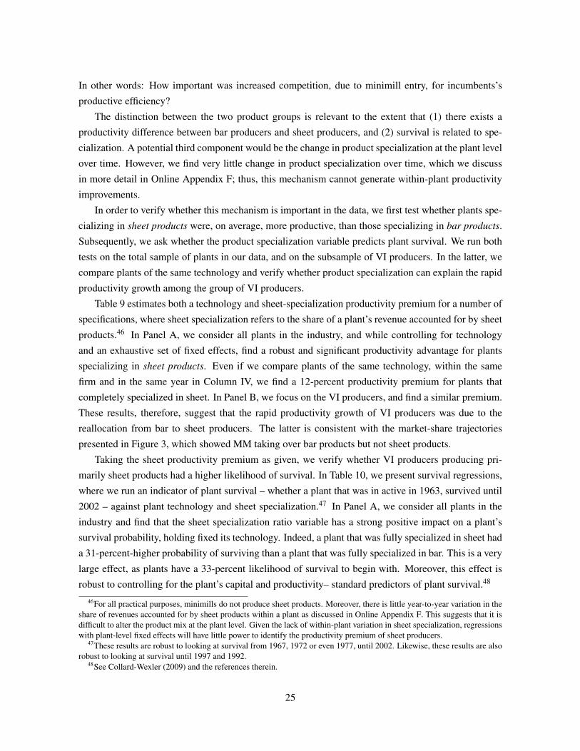
In other words: How important was increased competition, due to minimill entry, for incumbents’s

productive efficiency?

The distinction between the two product groups is relevant to the extent that (1) there exists a

productivity difference between bar producers and sheet producers, and (2) survival is related to spe-

cialization. A potential third component would be the change in product specialization at the plant level

over time. However, we find very little change in product specialization over time, which we discuss

in more detail in Online Appendix F; thus, this mechanism cannot generate within-plant productivity

improvements.

In order to verify whether this mechanism is important in the data, we first test whether plants spe-

cializing in sheet products were, on average, more productive, than those specializing in bar products.

Subsequently, we ask whether the product specialization variable predicts plant survival. We run both

tests on the total sample of plants in our data, and on the subsample of VI producers. In the latter, we

compare plants of the same technology and verify whether product specialization can explain the rapid

productivity growth among the group of VI producers.

Table 9 estimates both a technology and sheet-specialization productivity premium for a number of

specifications, where sheet specialization refers to the share of a plant’s revenue accounted for by sheet

products.46 In Panel A, we consider all plants in the industry, and while controlling for technology

and an exhaustive set of fixed effects, find a robust and significant productivity advantage for plants

specializing in sheet products. Even if we compare plants of the same technology, within the same

firm and in the same year in Column IV, we find a 12-percent productivity premium for plants that

completely specialized in sheet. In Panel B, we focus on the VI producers, and find a similar premium.

These results, therefore, suggest that the rapid productivity growth of VI producers was due to the

reallocation from bar to sheet producers. The latter is consistent with the market-share trajectories

presented in Figure 3, which showed MM taking over bar products but not sheet products.

Taking the sheet productivity premium as given, we verify whether VI producers producing pri-

marily sheet products had a higher likelihood of survival. In Table 10, we present survival regressions,

where we run an indicator of plant survival – whether a plant that was in active in 1963, survived until

2002 – against plant technology and sheet specialization.47 In Panel A, we consider all plants in the

industry and find that the sheet specialization ratio variable has a strong positive impact on a plant’s

survival probability, holding fixed its technology. Indeed, a plant that was fully specialized in sheet had

a 31-percent-higher probability of surviving than a plant that was fully specialized in bar. This is a very

large effect, as plants have a 33-percent likelihood of survival to begin with. Moreover, this effect is

robust to controlling for the plant’s capital and productivity– standard predictors of plant survival.48

46For all practical purposes, minimills do not produce sheet products. Moreover, there is little year-to-year variation in theshare of revenues accounted for by sheet products within a plant as discussed in Online Appendix F. This suggests that it isdifficult to alter the product mix at the plant level. Given the lack of within-plant variation in sheet specialization, regressionswith plant-level fixed effects will have little power to identify the productivity premium of sheet producers.

47These results are robust to looking at survival from 1967, 1972 or even 1977, until 2002. Likewise, these results are alsorobust to looking at survival until 1997 and 1992.

48See Collard-Wexler (2009) and the references therein.

25

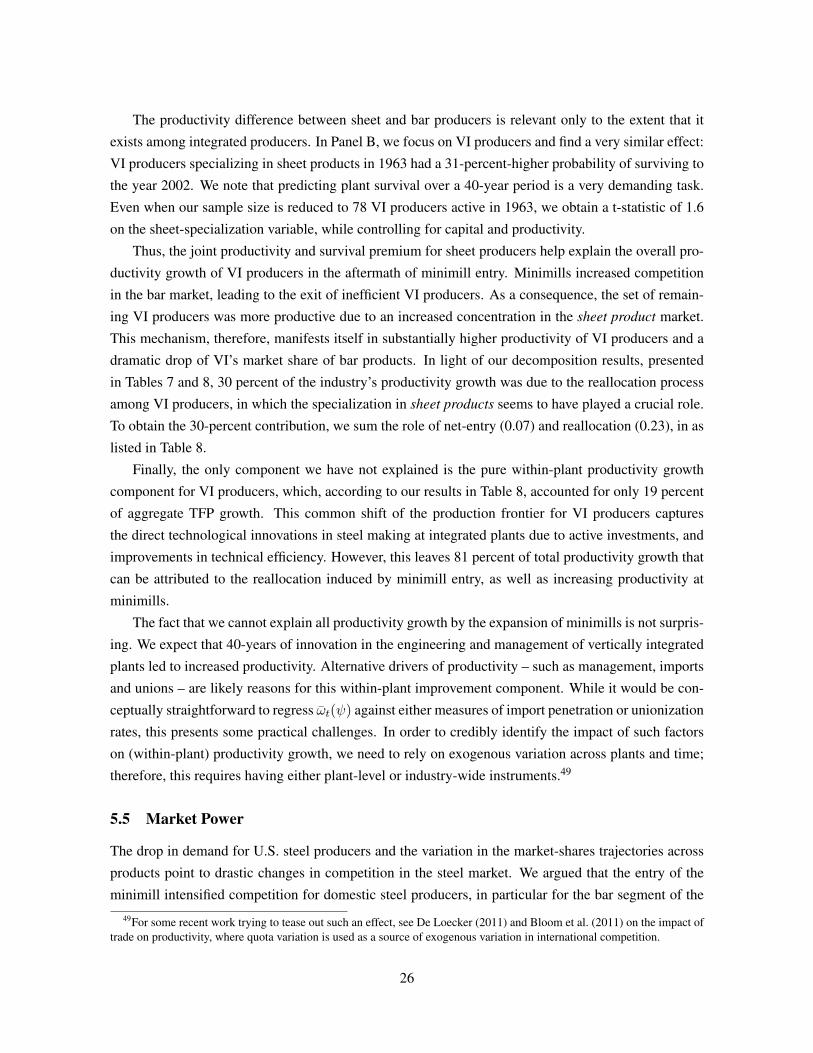
The productivity difference between sheet and bar producers is relevant only to the extent that it

exists among integrated producers. In Panel B, we focus on VI producers and find a very similar effect:

VI producers specializing in sheet products in 1963 had a 31-percent-higher probability of surviving to

the year 2002. We note that predicting plant survival over a 40-year period is a very demanding task.

Even when our sample size is reduced to 78 VI producers active in 1963, we obtain a t-statistic of 1.6

on the sheet-specialization variable, while controlling for capital and productivity.

Thus, the joint productivity and survival premium for sheet producers help explain the overall pro-

ductivity growth of VI producers in the aftermath of minimill entry. Minimills increased competition

in the bar market, leading to the exit of inefficient VI producers. As a consequence, the set of remain-

ing VI producers was more productive due to an increased concentration in the sheet product market.

This mechanism, therefore, manifests itself in substantially higher productivity of VI producers and a

dramatic drop of VI’s market share of bar products. In light of our decomposition results, presented

in Tables 7 and 8, 30 percent of the industry’s productivity growth was due to the reallocation process

among VI producers, in which the specialization in sheet products seems to have played a crucial role.

To obtain the 30-percent contribution, we sum the role of net-entry (0.07) and reallocation (0.23), in as

listed in Table 8.

Finally, the only component we have not explained is the pure within-plant productivity growth

component for VI producers, which, according to our results in Table 8, accounted for only 19 percent

of aggregate TFP growth. This common shift of the production frontier for VI producers captures

the direct technological innovations in steel making at integrated plants due to active investments, and

improvements in technical efficiency. However, this leaves 81 percent of total productivity growth that

can be attributed to the reallocation induced by minimill entry, as well as increasing productivity at

minimills.

The fact that we cannot explain all productivity growth by the expansion of minimills is not surpris-

ing. We expect that 40-years of innovation in the engineering and management of vertically integrated

plants led to increased productivity. Alternative drivers of productivity – such as management, imports

and unions – are likely reasons for this within-plant improvement component. While it would be con-

ceptually straightforward to regress ωt(ψ) against either measures of import penetration or unionization

rates, this presents some practical challenges. In order to credibly identify the impact of such factors

on (within-plant) productivity growth, we need to rely on exogenous variation across plants and time;

therefore, this requires having either plant-level or industry-wide instruments.49

5.5 Market Power

The drop in demand for U.S. steel producers and the variation in the market-shares trajectories across

products point to drastic changes in competition in the steel market. We argued that the entry of the

minimill intensified competition for domestic steel producers, in particular for the bar segment of the49For some recent work trying to tease out such an effect, see De Loecker (2011) and Bloom et al. (2011) on the impact of

trade on productivity, where quota variation is used as a source of exogenous variation in international competition.

26

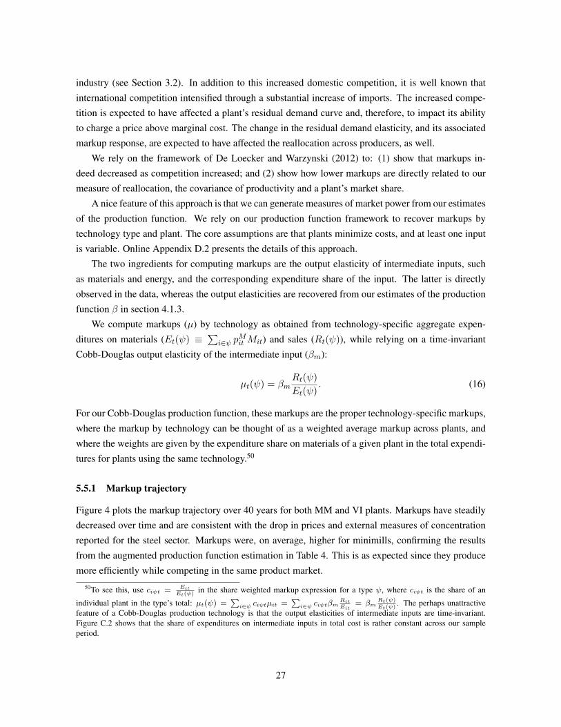
industry (see Section 3.2). In addition to this increased domestic competition, it is well known that

international competition intensified through a substantial increase of imports. The increased compe-

tition is expected to have affected a plant’s residual demand curve and, therefore, to impact its ability

to charge a price above marginal cost. The change in the residual demand elasticity, and its associated

markup response, are expected to have affected the reallocation across producers, as well.

We rely on the framework of De Loecker and Warzynski (2012) to: (1) show that markups in-

deed decreased as competition increased; and (2) show how lower markups are directly related to our

measure of reallocation, the covariance of productivity and a plant’s market share.

A nice feature of this approach is that we can generate measures of market power from our estimates

of the production function. We rely on our production function framework to recover markups by

technology type and plant. The core assumptions are that plants minimize costs, and at least one input

is variable. Online Appendix D.2 presents the details of this approach.

The two ingredients for computing markups are the output elasticity of intermediate inputs, such

as materials and energy, and the corresponding expenditure share of the input. The latter is directly

observed in the data, whereas the output elasticities are recovered from our estimates of the production

function β in section 4.1.3.

We compute markups (µ) by technology as obtained from technology-specific aggregate expen-

ditures on materials (Et(ψ) ≡∑

i∈ψ pMit Mit) and sales (Rt(ψ)), while relying on a time-invariant

Cobb-Douglas output elasticity of the intermediate input (βm):

µt(ψ) = βmRt(ψ)

Et(ψ). (16)

For our Cobb-Douglas production function, these markups are the proper technology-specific markups,

where the markup by technology can be thought of as a weighted average markup across plants, and

where the weights are given by the expenditure share on materials of a given plant in the total expendi-

tures for plants using the same technology.50

5.5.1 Markup trajectory

Figure 4 plots the markup trajectory over 40 years for both MM and VI plants. Markups have steadily

decreased over time and are consistent with the drop in prices and external measures of concentration

reported for the steel sector. Markups were, on average, higher for minimills, confirming the results

from the augmented production function estimation in Table 4. This is as expected since they produce

more efficiently while competing in the same product market.

50To see this, use ciψt = EitEt(ψ)

in the share weighted markup expression for a type ψ, where ciψt is the share of an

individual plant in the type’s total: µt(ψ) =∑i∈ψ ciψtµit =

∑i∈ψ ciψtβm

RitEit

= βmRt(ψ)Et(ψ)

. The perhaps unattractivefeature of a Cobb-Douglas production technology is that the output elasticities of intermediate inputs are time-invariant.Figure C.2 shows that the share of expenditures on intermediate inputs in total cost is rather constant across our sampleperiod.

27

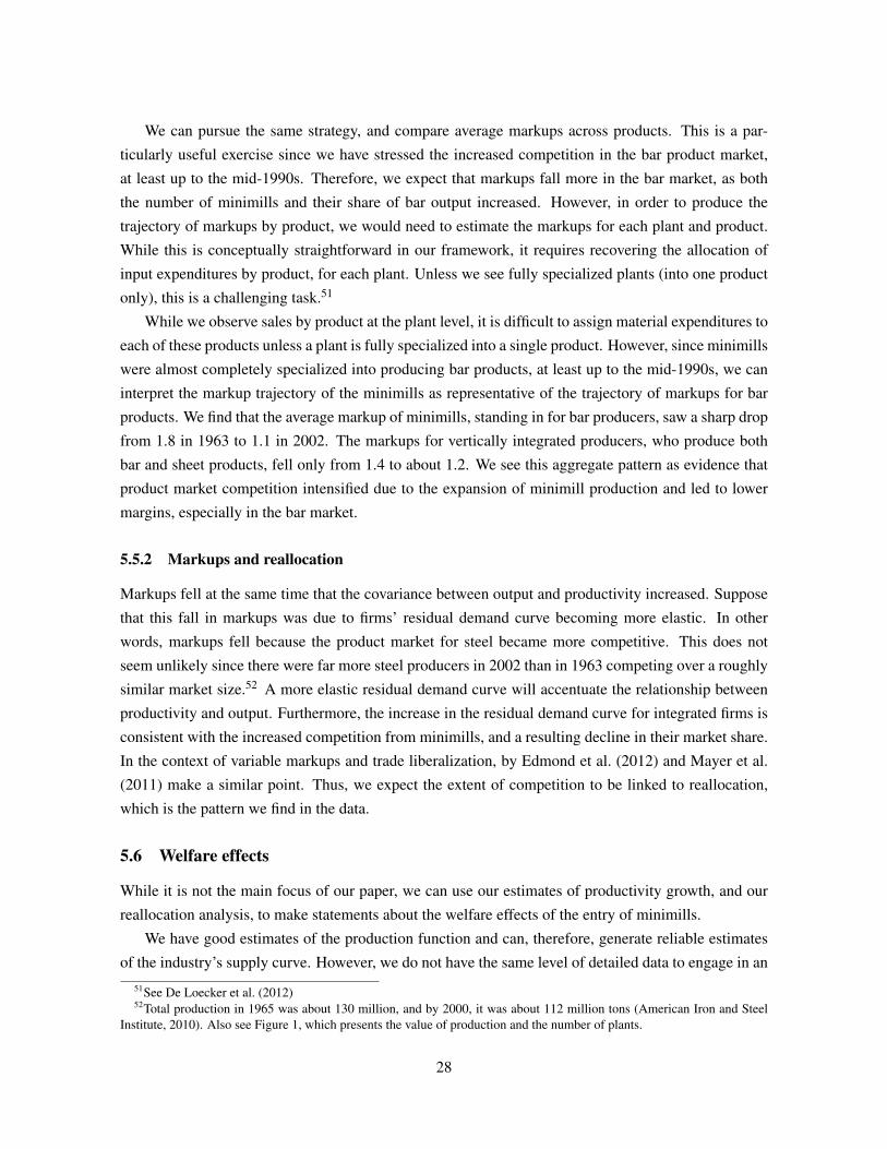
We can pursue the same strategy, and compare average markups across products. This is a par-

ticularly useful exercise since we have stressed the increased competition in the bar product market,

at least up to the mid-1990s. Therefore, we expect that markups fall more in the bar market, as both

the number of minimills and their share of bar output increased. However, in order to produce the

trajectory of markups by product, we would need to estimate the markups for each plant and product.

While this is conceptually straightforward in our framework, it requires recovering the allocation of

input expenditures by product, for each plant. Unless we see fully specialized plants (into one product

only), this is a challenging task.51

While we observe sales by product at the plant level, it is difficult to assign material expenditures to

each of these products unless a plant is fully specialized into a single product. However, since minimills

were almost completely specialized into producing bar products, at least up to the mid-1990s, we can

interpret the markup trajectory of the minimills as representative of the trajectory of markups for bar

products. We find that the average markup of minimills, standing in for bar producers, saw a sharp drop

from 1.8 in 1963 to 1.1 in 2002. The markups for vertically integrated producers, who produce both

bar and sheet products, fell only from 1.4 to about 1.2. We see this aggregate pattern as evidence that

product market competition intensified due to the expansion of minimill production and led to lower

margins, especially in the bar market.

5.5.2 Markups and reallocation

Markups fell at the same time that the covariance between output and productivity increased. Suppose

that this fall in markups was due to firms’ residual demand curve becoming more elastic. In other

words, markups fell because the product market for steel became more competitive. This does not

seem unlikely since there were far more steel producers in 2002 than in 1963 competing over a roughly

similar market size.52 A more elastic residual demand curve will accentuate the relationship between

productivity and output. Furthermore, the increase in the residual demand curve for integrated firms is

consistent with the increased competition from minimills, and a resulting decline in their market share.

In the context of variable markups and trade liberalization, by Edmond et al. (2012) and Mayer et al.

(2011) make a similar point. Thus, we expect the extent of competition to be linked to reallocation,

which is the pattern we find in the data.

5.6 Welfare effects

While it is not the main focus of our paper, we can use our estimates of productivity growth, and our

reallocation analysis, to make statements about the welfare effects of the entry of minimills.

We have good estimates of the production function and can, therefore, generate reliable estimates

of the industry’s supply curve. However, we do not have the same level of detailed data to engage in an51See De Loecker et al. (2012)52Total production in 1965 was about 130 million, and by 2000, it was about 112 million tons (American Iron and Steel

Institute, 2010). Also see Figure 1, which presents the value of production and the number of plants.

28

econometric analysis of the industry’s demand curve.

With this caveat in mind, we calculate the change in consumer surplus by presenting consumers

in 1963 with 2002 prices. We previously found that, at a minimum, 51 percent of productivity growth

could be attributed to the entry of minimills: 23 percent coming from the between reallocation (Table

7) and 28 percent coming from total minimill productivity growth (Table 8). Thus, we attribute 51

percent of the fall in prices for steel from 1963 to 2002 to minimills. We extrapolate counterfactual

demand under these 2002 prices using various assumptions of the elasticity of demand. Table B.9 in

the Online Appendix presents the consumer surplus gain in 1997 dollars, and the associated share of

this change in consumer surplus over total sales of the industry. We also compute the total change in

consumer surplus due to the fall in prices for steel from 1963 to 2002, irrespective of whether these are

due to minimill entry or some other factors.

Depending on the exact elasticity of demand that we assume, we find that consumer surplus in-

creased by between 17 and 23 billion dollars (in 1997 $) between 1963 and 2002. If we attribute

51 percent of this fall in prices to minimills, then minimills would be responsible for an increase in

consumer surplus of between nine and 11 billion dollars. Put differently, our back-of-the-envelope

calculations suggest that the reallocation towards minimills led to an increase in consumer surplus of

between 13 and 16 percent of shipments in the steel industry.

Of course, this somewhat crude welfare analysis leaves out several important issues, one of which

we already mentioned: We hold demand fixed, and impose a specific curvature of the demand curve.

Another omission from this analysis is that over 400,000 workers left the industry, and we do not take

into account the welfare implications of such a major transition.53 A more complete welfare analysis

should address these issues.

6 Robustness Analysis

We present the main results from our decomposition analysis using a variety of productivity estimates

(as presented in Table 4). We discuss the robustness of our results and highlight the importance of our

corrections in establishing a prominent role of technology in generating aggregate productivity growth.

Finally, we consider an alternative measure of aggregate productivity, and its associated decomposition,

which differs in the sense that reallocation can impact aggregate productivity only if the marginal

product of inputs are not equalized across producers.

6.1 Robustness

Tables 11 and 12 present robustness checks on our decompositions of aggregate productivity growth.

For several of the productivity estimates from using the specifications listed in Table 4, we produce53Our data do not track employment out of the steel industry. Data from the LEHD program (Abowd et al., 2004) could

presumably aid in identifying the reallocation of workers in the steel industry to other sectors.

29

the static and dynamic decompositions. The first column of Tables 11 and 12 rely on productivity es-

timates obtained using the production function coefficients of specification I in Table 4. We contrast

these to results obtained using productivity estimates obtained without correcting for simultaneity and

selection (Column II), and those obtained without correcting for unobserved output and input price dif-

ferences across producers (Columns III and IV). We also include the results using technology-specific

production functions (Column V), as discussed in Section 4.1.3 and presented in Column IV of Table

3.

The various components of the decompositions use plant-level estimates of productivity β, which

rely on estimated production function coefficients and, thus, are also estimates. We use a block boot-

strap routine to produce confidence intervals of the shares of each component. The 95-percent confi-

dence intervals are given in Tables 11 and 12. Note that the main points on reallocation that we have

discussed – such as the importance of the between covariance, the relatively faster growth of vertically

integrated plants relative to minimills, and the more important role of reallocation and net entry for

vertically integrated plants than for minimills – are statistically significantly at the 95-percent level for

our baseline specification in Column I.

6.2 Importance of Corrections

Looking across the columns of Tables 11 and 12 shows that to obtain the correct quantitative effects of

the entry of minimills on aggregate productivity, it is import to correct for unobserved productivity and

prices when estimating the production function. What is particularly sensitive to the specification of

the production function is the between decomposition. Indeed, the between component is 23 percent in

Column I, which uses GMM, as opposed to ten percent in Column II, using OLS productivity estimates.

These differences are statistically significant, as the 95-percent confidence intervals for the between

technology share do not overlap. This is unsurprising, as Table 4 showed that the minimill productivity

premium was far larger in Column I (GMM) than in Column II (OLS). These difference in the estimated

productivity advantages of minimills spill over directly to the estimated magnitude of the between

covariance. Likewise, if we had not controlled for plant-specific output prices, as shown by Column

IV, we would have found a between technology share of 18 percent rather than 23 percent, even though

this difference is not statistically significant. Again, the difference in the estimate between technology

share reflects differences in the estimated minimill premium found in Table 4.

The role of entry and exit is altered by not correcting for plant-level prices and productivity errors in

the production function. The impact of the exit process of vertically integrated producers is cut in half

(from 16 to seven percent between Columns I and II), while the within-plant minimill improvements are

underestimated (123 versus 87 percent from Column I to II). Correcting for simultaneity and selection

is crucial to obtain reliable productivity measures and, more importantly, to measure the impact of entry

and exit, an important part of our reallocation mechanism, on aggregate productivity.

Summing up, if we incorrectly ignored price variation across producers, the endogeneity of inputs,

and the non-random exit of plants in the data, we would underestimate the reallocation mechanism by

30

a factor of two. Our results suggest that the total effect of minimill entry on industry-wide productivity

growth was 81 percent. This share drops somewhat when ignoring unobserved price and productivity

heterogeneity. However, although we find a much larger magnitude, the role of technology is present

even when using uncorrected productivity estimates, which adds to the robustness of the importance of

our specific reallocation mechanism.

Allowing for technology-specific output elasticities, as shown in Column V, leads to virtually iden-

tical estimates of productivity growth and reallocation to those in Column I, which assume identical

output elasticities across the two technologies. However, the 95-percent confidence interval around

the various components is far larger in Column V than in Column I. This is to be expected given the

insignificant interaction terms between inputs and the vertically integrated dummy in Table 3, as well

as the associated loss in power when allowing for a more flexible production function.

6.3 Alternative decompositions

Recent work by Petrin and Levinsohn (2012) (PL hereafter) has highlighted that not all measures of ag-

gregate productivity, and their associated analysis of reallocation, can be mapped into either aggregate

GDP or welfare. While we are primarily interested in documenting the performance of one industry,

the U.S. steel industry, we do so using an intuitive and frequently used set of decompositions. At the

core of the concerns raised by PL is that the Olley-Pakes style aggregate productivity and the associated

reallocation, do not evaluate the use of inputs at their marginal products. In the extreme case, if the

marginal products of all inputs are equated across plants and, hence, in the absence of any frictions or

wedges between marginal products and input prices, there cannot be any role for reallocating resources

to more-productive plants.

In order to deal with this potential concern, we closely follow Petrin and Levinsohn (2012)’s ap-

proach to creating alternative decompositions of productivity growth.54 We first cast our decomposition

into the PL framework and discuss the measurement and implementation issues. Finally, we compute

the PL decomposition and verify the robustness of our main results, rather than pursuing a detailed

analysis of when and why these decompositions yield different results.55

6.3.1 Comparing both measures

The setup of PL is quite general, and we start by introducing the specifics of our application. First, we

rely on a Cobb-Douglas production, which implies that output elasticities for each input are constant

across plants and time, much like the application considered by PL.

A thorny issue is the treatment of capital. While PL work out the case for all inputs, in practice, we

face the challenge of how to measure the user cost of capital. If we ignore the contribution of capital54We rely on PL’s code downloaded from http://www.econ.umn.edu/˜petrin/programs.html, accessed

August 30, 2013.55The specific comparison with Olley-Pakes type decompositions has been done carefully and in great length by PL and

subsequent work Nishida et al. (2013b,a).

31

stock to aggregate productivity growth (APG hereafter), this will bias our results, both because capital

stock changed dramatically in this industry, and because vertically integrated plants and minimills have

different capital intensities. Thus, we treat labor and capital as inputs into production in our PL-style

productivity decompositions.56

Starting from PL’s equation (9) on page 711, and letting h index our inputs (l, k), we multiply and

divide by total revenue in the industry (∑

i PiQi), yielding aggregate productivity growth between t−1

and t as:

APGt =∑i

PiQi∑i PiQi

∑i PiQi∑i V Ai

∆ωit +∑i

PiQi∑i PiQi

∑i PiQi∑i V Ai

∑h

(βh − sih)∆hit

= θ∑i

msi∆ωit︸ ︷︷ ︸TE

+ θ∑i

msi∑h

(βh − sih)∆hit︸ ︷︷ ︸RE

, (17)

where all variables without a subscript it are approximated with the midpoint between their values at

times t and t− 1, and θ ≡∑i PiQi∑i V Ai

(Domar weight for the steel industry), and ∆hit = lnhit− lnhit−1

where lower cases denote logs.

The second line of equation (17) shows that APG can be decomposed into a Technical Efficiency

(TE) component and a reallocation component (RE). The TE term is our plant improvement compo-

nent in equation (15) up to a scaling by θ. This rescaling will not affect our analysis of the share of

productivity growth coming from reallocation versus technical efficiency.57

Given our previous analysis, we can already say a lot about the various components in the PL

decomposition in equation (17). First, while materials can be thought of as a flexible input that is

free from any frictions, we do allow for an imperfectly competitive output market. This imperfect

competition is plausible given the positive markups we found in Section 5.5.1. Thus, we should expect

there to be a wedge between an input’s output elasticity and the revenue share. For materials, our

variable input, the markup drives a wedge between the material revenue share and the firm’s output

elasticity. Second, for labor and capital, which we allow to face adjustment costs, this wedge will

be non-zero, irrespectively of whether there is imperfect competition in either the output or the input

market.58 This implies that there is the potential for the reallocation term in the PL framework to lead

to aggregate productivity growth: The movement of inputs across producers with different markups

and adjustment costs is a clear potential mechanism. Finally, from the raw data, as presented in Table

1 and Figure 1, we know that total employment dropped dramatically over the sample period, from

500,000 to 100,000. Moreover, the drop was almost entirely at integrated plants. Therefore, we expect

an important role of labor in when we break down the PL-reallocation term into the labor and capital.56This implies that we need to insert a user cost of capital to measure the share of the expenditure on capital in total value

added. We use a value of 12 percent and verify the robustness of our results using different values.57There is also a slight difference between our plant improvement term and PL due to the discrete nature of the data. In

PL, the midpoint of market share is used, while we rely on the lagged value.58See an extensive discussion of the wedge for inputs with adjustment costs, and their welfare implications in a dynamic

context, in Asker et al. (2013).

32

6.3.2 Robust role of technology

To compute the APG for the industry, the left-hand side of equation (17), we need to deal with various

implementation issues. First, we know that there is substantial entry and exit across plants of different

technologies. Second, we need to approximate the continuous-time setup of PL to a discrete-time

analogue. In addition, plant-specific cost shares are inherently noisy.59 This leads us to the following

equation that we take to our data:60

APGt = ∆ ln(∑i

V Ait)−∑L,K

[∑i∈A

aHi ∆hit +∑i∈B

aHit −∑i∈C

aHit−1

](18)

where aHi is the share of an input H’s expenditure in the industry’s total output V A (value added) with

H = L,K the input in levels, and A, B and C denotes continuers, entrants, and exiters, respectively.

The reallocation term RE is then simply recovered using the identity: REt = APGt − TEt.Table 13 presents the PL-decomposition of Aggregate Productivity Growth, for both the entire in-

dustry, and separately for minimills and vertically integrated plants. We show both the total productivity

growth in the steel industry (APG), as well as the shares accounted for by technical efficiency (TE), and

reallocation (RE). We also present the components of reallocation that can be attributed to the realloca-

tion of labor and capital. In the bottom panel of Table 13, we also reproduce the share of productivity

growth accounted for by the within and covariance terms in the Olley-Pakes decomposition.

PL’s measure of APG for the steel industry is 59 percent, while in our prior analysis, we found

aggregate productivity growth of 22 percent. These numbers may appear to be incompatible, but it is

important to notice that PL use a value-added metric for productivity, while we have employed a gross-

output measure. Since the Domar weight for the steel industry (the ratio of output to value added) is

about 2.5, this explains the discrepancy between these two measures of productivity growth.

The PL decomposition finds that 67 percent of productivity growth can be accounted for by tech-

nical efficiency, while the remaining 33 percent is due to reallocation. Our previous Olley-Pakes de-

compositions allocated 71 percent of productivity growth to the within component and 29 percent to

the covariance term. Thus, it seems that, for our industry, the two approaches agree as to the role of

reallocation of resources in explaining aggregate productivity growth. Indeed, once we account for

sampling error in output elasticities β, we find overlapping 95-percent confidence intervals for these

decompositions.

Likewise, once we drill down to the technology level, we also find a similar share of productivity

growth accounted for by within-plant effects and reallocation between plants by the PL and Olley-

Pakes approaches. For vertically integrated plants, the TE component is 74 percent, while the within

component is 83 percent. For minimills, these numbers are 57 percent and 55 percent, respectively.59See the discussion in De Loecker and Warzynski (2012) on the need to correct the revenue shares as the raw data might,

for instance, lead to the wage bill over sales to lie anywhere from zero to a very large number. These plant-level shares areinteracted with plant-level changes in input use, and this noise in revenue shares can have large implications.

60See Section 7 in PL on the specifics of the discrete-time approximation for more detail on the derivation of this equation.

33

When applying the PL decomposition by technology, we find that the reallocation component for

integrated producers is substantial and that the labor term is large and negative at -26 percent. To

understand this effect, note that with a positive markup, any reduction in total output will be damaging

in terms of efficiency, as the market power induced quantity distortion is further accentuated. Thus,

even if the labor share sli and the output elasticity of labor βl are identical across all plants, when labor

falls among vertically integrated plants, this shows up as a negative reallocation term. Likewise, there is

a positive labor reallocation term for minimills of 11 percent, since minimills expanded their workforce

over the time period.

This logic does not directly translate to inputs that face substantial adjustment costs, such as capital,

where the wedge contains both markups and adjustment costs. We find that the capital accounts for 13

percent of APG, indicating that capital reallocation had a large role in efficiency gains for the industry.

We refer the reader to PL for a more thorough discussion of the interpretation of the capital reallocation

component.

Finally, just as in our previous discussion of static decompositions of productivity growth, we know

that plant entry and exit will confound the interpretation of the within and reallocation terms. This is

equally true of our PL decompositions, but given the continuous time approximation, we do not pursue

this analysis, and we appeal to our previous results on the importance of entry and exit.

7 Conclusion

There is, by now, extensive evidence that reallocation of resources across producers substantially im-

pacts productivity growth. This paper is one of the first to provide a specific mechanism underlying

such reallocation: The entry of a new technology, the minimill, and its associated increased competi-

tion, were largely responsible for the massive productivity growth in the U.S. steel industry.

We provide evidence that technological change can, by itself, bring about a process of resource

reallocation over a long period of time and lead to substantial productivity growth for the industry as

a whole. We find that the introduction of a new production technology spurred productivity growth

through two channels.

First, the entry of minimills led to a slow but steady drop in the market share of the incumbent

technology – the vertically integrated producers. As minimills were 7.5-percent more productive, this

movement of market share between technologies was responsible for a third of the industry’s produc-

tivity growth. Second, the old technology had faster growth in productivity than the new technology,

with TFP growth of 24 percent for vertically integrated producers versus only ten percent for minimills.

This catching-up process of the incumbents came about from a large within reallocation of resources

among vertically integrated plants.

The reallocation among vertically integrated plants was largely due the exit of inefficient producers

active in the low-quality segment (bar products.) On the other hand, minimills’ productivity increased

gradually over time due to a shift in the production function for all minimill producers. Although the

34

first mimimill producing at a commercial level, entered in the late 1950s, the productivity effects were

long-lasting and still affect the industry’s performance today. In fact, the recent trend in market shares

suggests that minimills have started to enter the high-quality segment of the industry – sheet products

– and taking our results at face value would indicate that more substantial productivity gains can be

expected.

Our results indicate that the arrival of new technologies can have a major impact on productive

efficiency through increased competition and its associated reallocation of economic resources, leading

to an increase in the industry’s overall performance. It is critical to obtain measures of plant-level

performance and technology to identify this mechanism – i.e., without indicators of technology at the

plant level, we would falsely attribute the productivity gains to other factors correlated with aggregate

productivity, such as international competition, geography, and a variety of firm-level characteristics.

References

ABOWD, J. M., J. HALTIWANGER, AND J. LANE (2004): “Integrated longitudinal employer-employee data for the United States,” The American Economic Review, 94, 224–229.

ACKERBERG, D., L. BENKARD, S. BERRY, AND A. PAKES (2007): “Econometric Tools for Analyz-ing Market Outcomes,” in Handbook of Econometrics, ed. by J. Heckman and E. Leamer, Elsevier,vol. 6a, chap. 63, 4171–4276.

AMERICAN IRON AND STEEL INSTITUTE (2010): Annual Statistical Report of the American Iron andSteel Institute, Washington D.C.

ARTHUR, J. B. (1999): “Explaining variation in human resource practices in US steel minimills,”in Employment Practices and Business Strategy, ed. by P. Cappelli, Oxford University Press, NewYork, chap. 1.

ASKER, J., A. COLLARD-WEXLER, AND J. DE LOECKER (2013): “Dynamic Inputs and Resource(Mis)Allocation,” Journal of Political Economy, forthcoming.

BARNETT, D. F. AND R. W. CRANDALL (1986): Up from the ashes: The rise of the steel minimill inthe United States, Brookings Institution Press.

BARTELSMAN, E., R. BECKER, AND W. GRAY (2000): “Nber-ces manufacturing industry database,”Last accessed May, 25, 2006.

BARTELSMAN, E., J. HALTIWANGER, AND S. SCARPETTA (2009): “Cross-country differences inproductivity: the role of allocation and selection,” Tech. rep., NBER Working Paper.

BENKARD, C. (2000): “Learning and Forgetting: The Dynamics of Aircraft Production,” AmericanEconomic Review, 90, 1034–1054.

BERNARD, A., J. JENSEN, AND P. SCHOTT (2006): “Survival of the best fit: Exposure to low-wagecountries and the (uneven) growth of US manufacturing plants,” Journal of International Economics,68, 219–237.

35

BLOOM, N., M. DRACA, AND J. VAN REENEN (2011): “Trade induced technical change? The impactof Chinese imports on innovation, IT and productivity,” Tech. rep., National Bureau of EconomicResearch.

BLOOM, N., B. EIFERT, A. MAHAJAN, D. MCKENZIE, AND J. ROBERTS (2013): “Does manage-ment matter? Evidence from India,” Quarterly Journal of Economics, 128, 1–51.

BLOOM, N. AND J. VAN REENEN (2010): “Why do management practices differ across firms andcountries?” The Journal of Economic Perspectives, 203–224.

BRESNAHAN, T. F. AND D. M. G. RAFF (1991): “Intra-Industry Heterogeneity and the Great Depres-sion: The American Motor Vehicles Industry, 1929-1935,” The Journal of Economic History, 51,317–331.

CLARK, K. B. (1980): “Unionization and productivity: Micro-econometric evidence,” The QuarterlyJournal of Economics, 95, 613–639.

COLLARD-WEXLER, A. (2009): “Productivity Dispersion and Plant Selection in the Ready-Mix Con-crete Industry,” Working Paper, New York University.

CRANDALL, R. (1981): The US steel industry in recurrent crisis: policy options in a competitiveworld, Brookings Institution Press.

DAVIS, S. J., J. C. HALTIWANGER, AND S. SCHUH (1996): Job creation and destruction, MIT PressCambridge, Mass.

DE LOECKER, J. (2011): “Product Differentiation, Multiproduct Firms, and Estimating the Impact ofTrade Liberalization on Productivity,” Econometrica, 79, 1407–1451.

DE LOECKER, J. AND P. GOLDBERG (2014): “Firm Performance in a Global Market Firm Perfor-mance in a Global Market Firm Performance in a Global Market,” Annual Review of Economics,6.

DE LOECKER, J., P. GOLDBERG, A. KHANDELWAL, AND N. PAVCNIK (2012): “Prices, Markupsand Trade Reform,” Tech. rep., National Bureau of Economic Research.

DE LOECKER, J. AND J. KONINGS (2006): “Job reallocation and productivity growth in a post-socialist economy: Evidence from Slovenian manufacturing,” European Journal of Political Econ-omy, 22, 388–408.

DE LOECKER, J. AND F. WARZYNSKI (2012): “Markups and firm-level export status,” AmericanEconomic Review, 102, 2437–2471.

EDMOND, C., V. MIDRIGAN, AND D. XU (2012): “Competition, markups, and the gains from inter-national trade,” Tech. rep., National Bureau of Economic Research.

FOSTER, L., J. HALTIWANGER, AND C. KRIZAN (2001): “Aggregate productivity growth. Lessonsfrom microeconomic evidence,” in New developments in productivity analysis, University of ChicagoPress.

FOSTER, L., J. HALTIWANGER, AND C. SYVERSON (2008): “Reallocation, Firm Turnover, and Effi-ciency: Selection on Productivity or Profitability?” American Economic Review, 98, 394–425.

36

FRUEHAN, R. (1998): The Making, Shaping and Treating of Steel - 11th Edition, AISE Steel Founda-tion, Pittsburgh, USA.

GIARRATANI, F., G. GRUVER, AND R. JACKSON (2007): “Clusters, agglomeration, and economic de-velopment potential: empirical evidence based on the advent of slab casting by US steel minimills,”Economic Development Quarterly, 21, 148–164.

HALL, C. (1997): Steel phoenix: The fall and rise of the US steel industry, Palgrave Macmillan.

HOERR, J. (1988): And the wolf finally came: The decline of the American steel industry, Universityof Pittsburgh Press Pittsburgh.

HORTACSU, A. AND C. SYVERSON (2004): “Cementing Relationships: Vertical Integration, Foreclo-sure, Productivity, and Prices,” .

ICHNIOWSKI, C., K. SHAW, AND G. PRENNUSHI (1997): “The Effects of Human Resource Manage-ment Practices on Productivity: A Study of Steel Finishing Lines,” American Economic Review, 87,291–313.

JARMIN, R., S. KLIMEK, AND J. MIRANDA (2009): “The Role of Retail Chains: National, Re-gional and Industry Results,” in Producer Dynamics: New Evidence from Micro Data, University ofChicago Press, 237–262.

LEE, D. S. AND A. MAS (2012): “Long-run impacts of unions on firms: New evidence from financialmarkets, 1961–1999,” The Quarterly Journal of Economics, 127, 333–378.

LEVINSOHN, J. AND A. PETRIN (2003): “Estimating Production Functions Using Inputs to Controlfor Unobservables,” Review of Economic Studies, 70, 317–341.

MAASOUMI, E., S. D. PROWSE, AND D. J. SLOTTJE (2002): “Measuring market power in the steelindustry,” Contributions to Economic Analysis, 255, 115–134.

MAYER, T., M. MELITZ, AND G. OTTAVIANO (2011): “Market size, competition, and the productmix of exporters,” Tech. rep., National Bureau of Economic Research.

MEDOFF, J. L. AND R. FREEMAN (1984): “What Do Unions Do,” New York.

MELITZ, M. (2003): “The impact of trade on intra-industry reallocations and aggregate industry pro-ductivity,” Econometrica, 1695–1725.

NISHIDA, M., A. PETRIN, AND S. POLANEC (2013a): “Exploring Reallocation s Apparent WeakContribution to Growth,” Tech. rep., National Bureau of Economic Research.

NISHIDA, M., A. PETRIN, AND T. K. WHITE (2013b): “Are We Undercounting Reallocation’s Con-tribution to Growth?” Tech. rep., University of Minnessota.

OLLEY, G. S. AND A. PAKES (1996): “The dynamics of productivity in the telecommunicationsequipment industry,” Econometrica, 64, 35.

OSTER, S. (1982): “The Diffusion of Innovation among Steel Firms: The Basic Oxygen Furnace,” TheBell Journal of Economics, 13, pp. 45–56.

37

PETRIN, A. AND J. LEVINSOHN (2012): “Measuring aggregate productivity growth using plant-leveldata,” The RAND Journal of Economics, 43, 705–725.

ROGERS, R. (2009): An economic history of the American steel industry, Taylor & Francis.

SCHMITZ, J. (2005): “What determines productivity? Lessons from the dramatic recovery of the USand Canadian iron ore industries following their early 1980s crisis,” Journal of Political Economy,113, 582–625.

SYVERSON, C. (2011): “What Determines Productivity?” Journal of Economic Literature, 49, 326–65.

VAN BIESEBROECK, J. (2003): “Productivity dynamics with technology choice: An application toautomobile assembly,” The Review of Economic Studies, 70, 167–198.

38

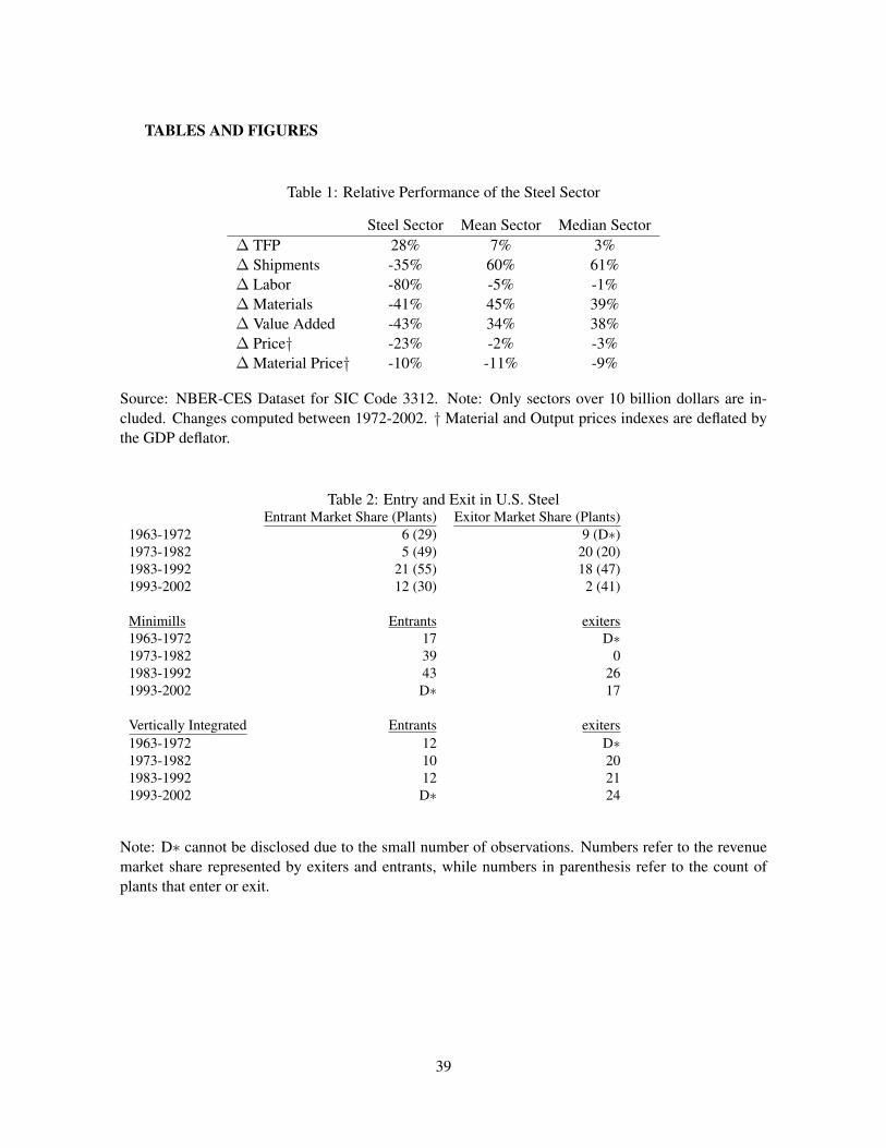
TABLES AND FIGURES

Table 1: Relative Performance of the Steel Sector

Steel Sector Mean Sector Median Sector∆ TFP 28% 7% 3%∆ Shipments -35% 60% 61%∆ Labor -80% -5% -1%∆ Materials -41% 45% 39%∆ Value Added -43% 34% 38%∆ Price† -23% -2% -3%∆ Material Price† -10% -11% -9%

Source: NBER-CES Dataset for SIC Code 3312. Note: Only sectors over 10 billion dollars are in-cluded. Changes computed between 1972-2002. † Material and Output prices indexes are deflated bythe GDP deflator.

Table 2: Entry and Exit in U.S. SteelEntrant Market Share (Plants) Exitor Market Share (Plants)

1963-1972 6 (29) 9 (D∗)1973-1982 5 (49) 20 (20)1983-1992 21 (55) 18 (47)1993-2002 12 (30) 2 (41)

Minimills Entrants exiters1963-1972 17 D∗1973-1982 39 01983-1992 43 261993-2002 D∗ 17

Vertically Integrated Entrants exiters1963-1972 12 D∗1973-1982 10 201983-1992 12 211993-2002 D∗ 24

Note: D∗ cannot be disclosed due to the small number of observations. Numbers refer to the revenuemarket share represented by exiters and entrants, while numbers in parenthesis refer to the count ofplants that enter or exit.

39

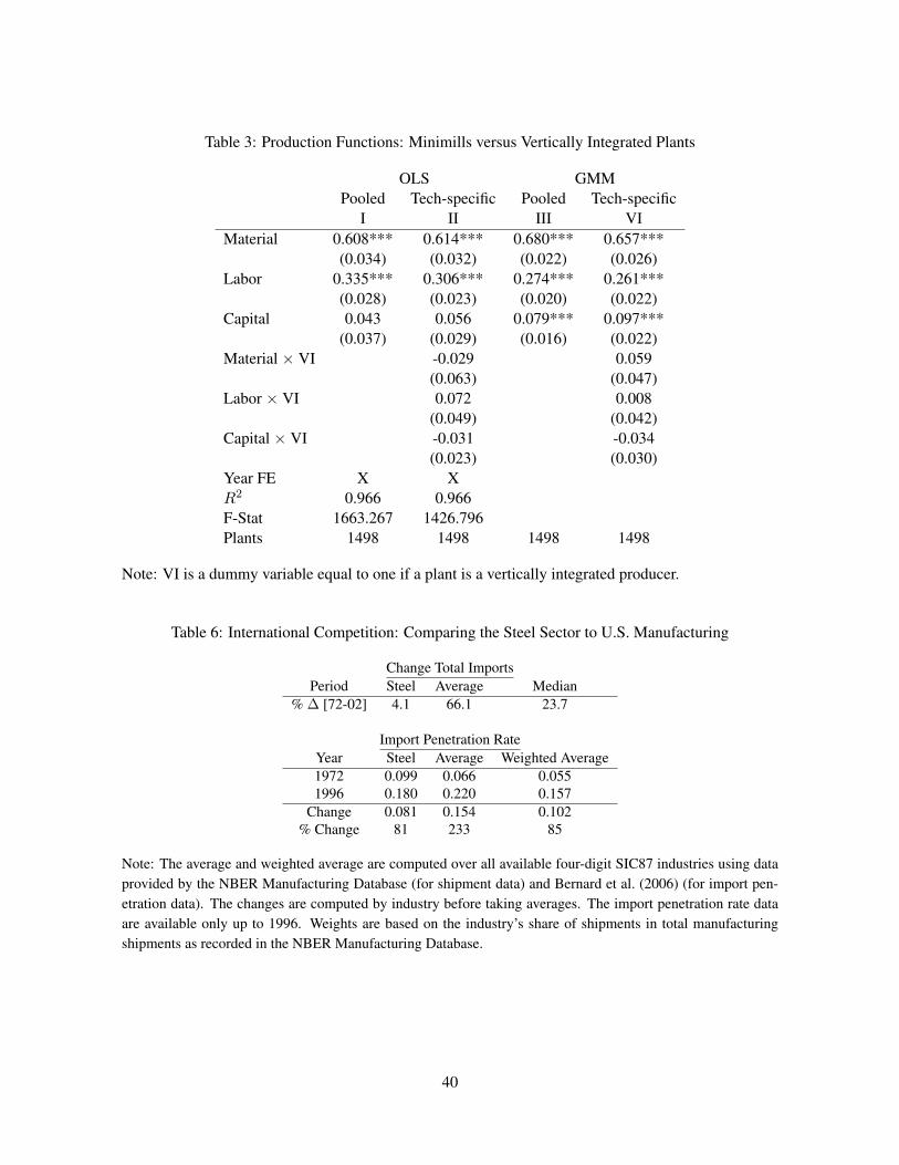
Table 3: Production Functions: Minimills versus Vertically Integrated Plants

OLS GMMPooled Tech-specific Pooled Tech-specific

I II III VIMaterial 0.608*** 0.614*** 0.680*** 0.657***

(0.034) (0.032) (0.022) (0.026)Labor 0.335*** 0.306*** 0.274*** 0.261***

(0.028) (0.023) (0.020) (0.022)Capital 0.043 0.056 0.079*** 0.097***

(0.037) (0.029) (0.016) (0.022)Material × VI -0.029 0.059

(0.063) (0.047)Labor × VI 0.072 0.008

(0.049) (0.042)Capital × VI -0.031 -0.034

(0.023) (0.030)Year FE X XR2 0.966 0.966F-Stat 1663.267 1426.796Plants 1498 1498 1498 1498

Note: VI is a dummy variable equal to one if a plant is a vertically integrated producer.

Table 6: International Competition: Comparing the Steel Sector to U.S. Manufacturing

Change Total ImportsPeriod Steel Average Median

% ∆ [72-02] 4.1 66.1 23.7

Import Penetration RateYear Steel Average Weighted Average1972 0.099 0.066 0.0551996 0.180 0.220 0.157

Change 0.081 0.154 0.102% Change 81 233 85

Note: The average and weighted average are computed over all available four-digit SIC87 industries using dataprovided by the NBER Manufacturing Database (for shipment data) and Bernard et al. (2006) (for import pen-etration data). The changes are computed by industry before taking averages. The import penetration rate dataare available only up to 1996. Weights are based on the industry’s share of shipments in total manufacturingshipments as recorded in the NBER Manufacturing Database.

40

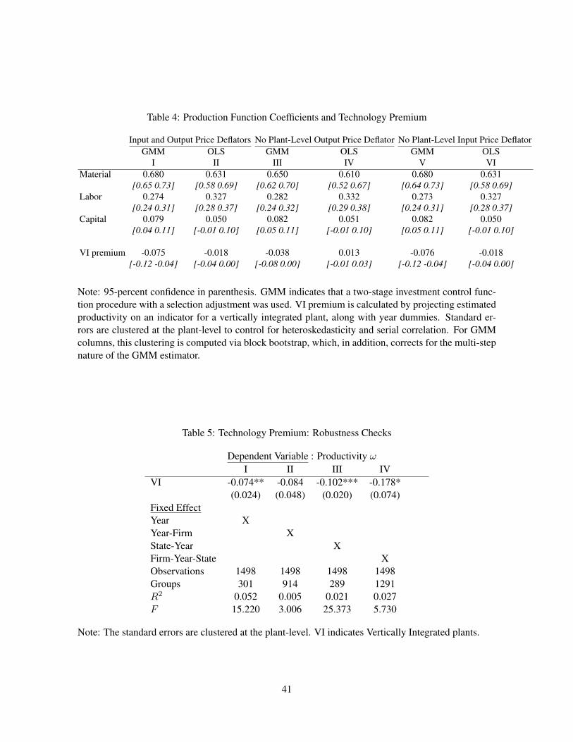
Table 4: Production Function Coefficients and Technology Premium

Input and Output Price Deflators No Plant-Level Output Price Deflator No Plant-Level Input Price DeflatorGMM OLS GMM OLS GMM OLS

I II III IV V VIMaterial 0.680 0.631 0.650 0.610 0.680 0.631

[0.65 0.73] [0.58 0.69] [0.62 0.70] [0.52 0.67] [0.64 0.73] [0.58 0.69]Labor 0.274 0.327 0.282 0.332 0.273 0.327

[0.24 0.31] [0.28 0.37] [0.24 0.32] [0.29 0.38] [0.24 0.31] [0.28 0.37]Capital 0.079 0.050 0.082 0.051 0.082 0.050

[0.04 0.11] [-0.01 0.10] [0.05 0.11] [-0.01 0.10] [0.05 0.11] [-0.01 0.10]

VI premium -0.075 -0.018 -0.038 0.013 -0.076 -0.018[-0.12 -0.04] [-0.04 0.00] [-0.08 0.00] [-0.01 0.03] [-0.12 -0.04] [-0.04 0.00]

Note: 95-percent confidence in parenthesis. GMM indicates that a two-stage investment control func-tion procedure with a selection adjustment was used. VI premium is calculated by projecting estimatedproductivity on an indicator for a vertically integrated plant, along with year dummies. Standard er-rors are clustered at the plant-level to control for heteroskedasticity and serial correlation. For GMMcolumns, this clustering is computed via block bootstrap, which, in addition, corrects for the multi-stepnature of the GMM estimator.

Table 5: Technology Premium: Robustness Checks

Dependent Variable : Productivity ωI II III IV

VI -0.074** -0.084 -0.102*** -0.178*(0.024) (0.048) (0.020) (0.074)

Fixed EffectYear XYear-Firm XState-Year XFirm-Year-State XObservations 1498 1498 1498 1498Groups 301 914 289 1291R2 0.052 0.005 0.021 0.027F 15.220 3.006 25.373 5.730

Note: The standard errors are clustered at the plant-level. VI indicates Vertically Integrated plants.

41

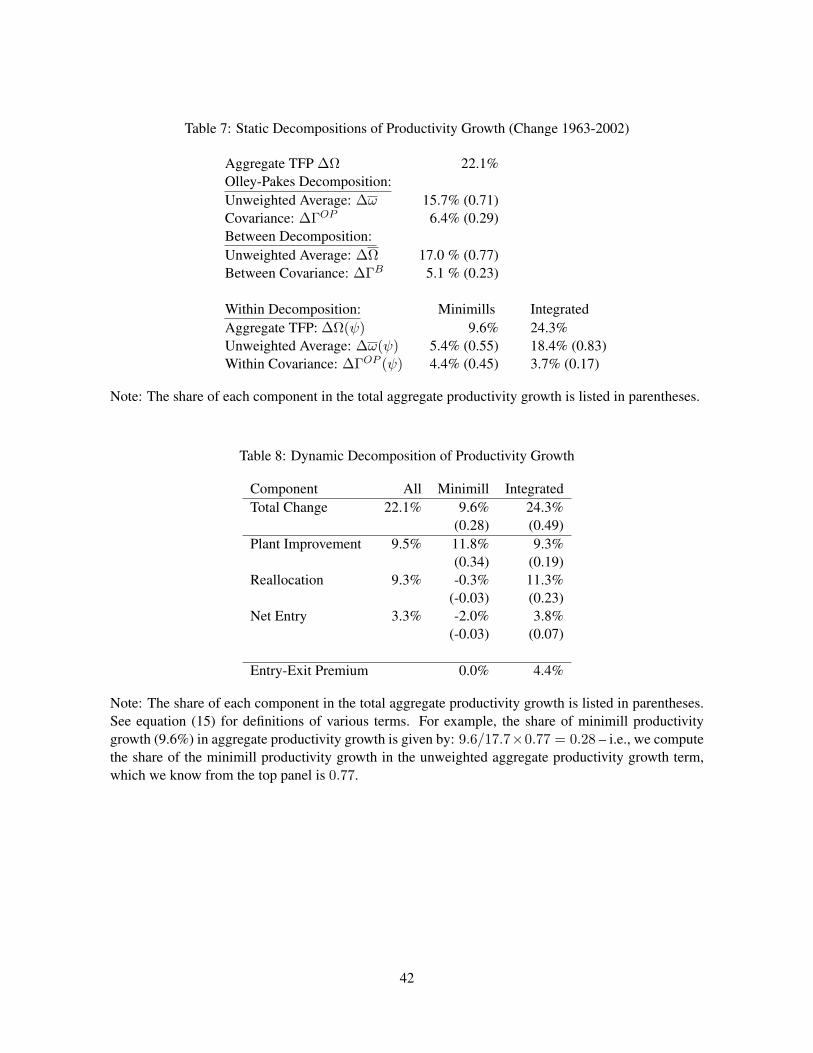
Table 7: Static Decompositions of Productivity Growth (Change 1963-2002)

Aggregate TFP ∆Ω 22.1%Olley-Pakes Decomposition:Unweighted Average: ∆ω 15.7% (0.71)Covariance: ∆ΓOP 6.4% (0.29)Between Decomposition:Unweighted Average: ∆Ω 17.0 % (0.77)Between Covariance: ∆ΓB 5.1 % (0.23)

Within Decomposition: Minimills IntegratedAggregate TFP: ∆Ω(ψ) 9.6% 24.3%Unweighted Average: ∆ω(ψ) 5.4% (0.55) 18.4% (0.83)Within Covariance: ∆ΓOP (ψ) 4.4% (0.45) 3.7% (0.17)

Note: The share of each component in the total aggregate productivity growth is listed in parentheses.

Table 8: Dynamic Decomposition of Productivity Growth

Component All Minimill IntegratedTotal Change 22.1% 9.6% 24.3%

(0.28) (0.49)Plant Improvement 9.5% 11.8% 9.3%

(0.34) (0.19)Reallocation 9.3% -0.3% 11.3%

(-0.03) (0.23)Net Entry 3.3% -2.0% 3.8%

(-0.03) (0.07)

Entry-Exit Premium 0.0% 4.4%

Note: The share of each component in the total aggregate productivity growth is listed in parentheses.See equation (15) for definitions of various terms. For example, the share of minimill productivitygrowth (9.6%) in aggregate productivity growth is given by: 9.6/17.7×0.77 = 0.28 – i.e., we computethe share of the minimill productivity growth in the unweighted aggregate productivity growth term,which we know from the top panel is 0.77.

42

Table 9: Sheet Productivity Premium

Dependent Variable: Productivity ωPanel A: All Plants Panel B: Vertically Integrated

I II III IV V VI VII VIII IX XVertically Integrated -0.080*** -0.082*** -0.115*** -0.089* -0.199**

(0.021) (0.024) (0.018) (0.036) (0.077)Sheet Specialization 0.073* 0.094*** 0.119** 0.078 0.058 0.099** 0.114* 0.168* 0.089Ratio (0.035) (0.025) (0.036) (0.068) (0.038) (0.032) (0.047) (0.084) (0.079)

Fixed EffectsYear X X X XState-Year X XFirm-Year X XFirm-State-Year X XPlant X

Observations 1498 1498 1498 1498 1498 667 667 667 667 667Number of FE 301 301 289 914 129 124 175 353 124 540R2 0.020 0.082 0.034 0.024 0.033 0.069 0.019 0.019 0.081 0.011F 14.639 17.167 21.143 7.019 3.537 7.944 9.290 5.980 5.214 1.263

Note: Standard Errors clustered by plant, but not corrected for the sampling error in constructed productivity.Sheet Specialization Ratio is the share of revenues accounted for by sheet products (hot and cold rolled sheet).

Table 10: Determinants of Exit

Dependent Variable: Plant Exists in 2002Panel A: All Plants Panel B: Vertically Integrated

I II III IV VVertically Integrated -0.36*** -0.39***

(0.09) (0.08)Sheet Specialization Ratio 0.39** 0.36* 0.31* 0.31* 0.22

(0.14) (0.14) (0.13) (0.13) (0.14)Log Capital (k) 0.02 0.20 0.24

(0.03) (0.24) (0.25)Productivity (ω) 0.03 0.05

(0.14) (0.04)

Observations 128 128 78 78 78Log-Likelihood -73.88 -73.72 -40.36 -40.02 -39.24χ2 16.97 17.30 5.89 6.58 8.12Baseline Probability 0.33 0.33 0.23 0.23 0.22

Note: Marginal Effects presented. Dependent variable is whether the plant has not exited by 2002 givenits status in 1963. Very similar results are found with 1972 and 1977 as base years.

43

Table 11: Static Decompositions under Alternative Productivity Measures

Baseline OLS No Material Price No Output Price Tech-SpecificDeflator Deflator Production Function

I II III IV VChange in TFP 22% 28% 22% 23% 19%

[0.17 0.27] [0.23 0.33] [0.16 0.27] [0.18 0.28] [0.01 0.27]Olley-PakesUnweighted Average (∆ω) 71% 69% 71% 77% 65%

[0.59 0.79] [0.62 0.73] [0.60 0.79] [0.68 0.84] [-0.01 0.87]Covariance (∆ΓOP ) 29% 32% 29% 23% 36%

[0.21 0.41] [0.27 0.38] [0.21 0.41] [0.16 0.32] [0.14 1.01]BetweenChange in Ω 77% 90% 76% 82% 81%

[0.68 0.83] [0.86 0.94] [0.68 0.83] [0.74 0.87] [0.52 2.50]Change in Between Technology 23% 10% 24% 18% 19%Covariance (∆ΓB) [0.17 0.32] [0.06 0.14] [0.17 0.33] [0.13 0.26] [-1.50 0.49]

Within TechnologyMinimillsChange in TFP 43% 74% 42% 50% 45%(ratio to aggregate ∆Ω(MM)

∆Ω ) [0.19 0.60] [0.59 0.85] [0.18 0.58] [0.29 0.63] [0.02 1.85]Fraction from Unweighted Average 55% 62% 55% 77% 55%(∆ω(MM)) [-0.02 0.70] [0.53 0.69] [-0.05 0.70] [0.59 0.86] [-0.05 0.77]Fraction from Covariance 45% 38% 45% 24% 45%(∆ΓOP (MM)) [0.31 1.02] [0.31 0.47] [0.30 1.05] [0.14 0.41] [0.23 1.05]Vertically IntegratedChange in TFP 110% 107% 111% 114% 118%(ratio to aggregate ∆Ω(V I)

∆Ω ) [1.03 1.21] [1.01 1.14] [1.03 1.22] [1.06 1.24] [0.78 3.24]Fraction from Unweighted Average 83% 76% 84% 89% 87%(∆ω(V I)) [0.73 0.94] [0.71 0.82] [0.74 0.94] [0.81 0.98] [0.73 1.02]Fraction from Covariance 17% 24% 17% 11% 13%(∆ΓOP (V I)) [0.06 0.27] [0.18 0.30] [0.06 0.26] [0.02 0.19] [-0.02 0.27]

Note: GMM refers to the Olley-Pakes control function approach. Plant-level output prices refers to deflatingrevenue using product-level price indexes. Plant-level material prices refers to deflating material inputs costsusing material specific price indexes. Bootstrapped 95-percent confidence intervals using 10,000 replications areshown in brackets, and these include only sampling error in the computation of productivity ω.

44

Table 12: Dynamic Decompositions under Alternative Productivity Measures

Baseline OLS No Material Price No Output Price Tech-SpecificDeflator Deflator Production Function

I II III IV VDynamic DecompositionAllPlant Improvement 43% 46% 43% 49% 47%

[0.35 0.49] [0.40 0.50] [0.34 0.49] [0.43 0.53] [0.20 1.15]Reallocation 42% 42% 42% 40% 43%

[0.35 0.54] [0.37 0.49] [0.35 0.54] [0.33 0.49] [0.30 0.83]Entry-Exit 15% 12% 15% 11% 10%

[0.12 0.18] [0.11 0.13] [0.12 0.18] [0.08 0.14] -[0.85 0.29]MinimillsPlant Improvement 123% 87% 125% 136% 124%

[0.94 2.59] [0.77 1.03] [0.94 2.68] [1.07 2.36] [0.88 2.59]Reallocation -3% 5% -3% -11% 9%

-[0.51 0.09] -[0.03 0.12] -[0.54 0.09] -[0.49 0.01] -[0.56 1.03]Entry-Exit -21% 8% -22% -25% -34%

-[1.08 0.00] -[0.02 0.14] -[1.18 -0.01] -[0.87 -0.07] -[1.92 0.04]Vertically IntegratedPlant Improvement 38% 40% 38% 42% 39%

[0.26 0.48] [0.33 0.46] [0.26 0.48] [0.32 0.51] [0.09 0.49]Reallocation 46% 54% 46% 46% 51%

[0.33 0.61] [0.47 0.61] [0.32 0.61] [0.34 0.59] [0.32 1.15]Entry-Exit 16% 7% 16% 12% 11%

[0.10 0.22] [0.05 0.09] [0.11 0.22] [0.07 0.17] -[0.35 0.29]

Note: GMM refers to the Olley-Pakes control function approach. Plant-level output prices refers to deflatingrevenue using product-level price indexes. Plant-level material prices refers to deflating material inputs costsusing material specific price indexes. Bootstrapped 95-percent confidence intervals using 10,000 replications areshown in brackets, and these include only sampling error in the computation of productivity ω.

Table 13: Alternative Decomposition

Sample APG Technical Efficiency (TE) Reallocation (RE) Labor RE Capital RESteel 0.59 67% 33% -16% 13%Vertically Integrated 0.59 74% 28% -26% 23%Minimill 0.61 57% 46% 11% -20%

Main Results from Table 7: Within and ReallocationSample Within CovarianceSteel 71% 29%Vertically Integrated 83% 17%Minimill 55% 45%

Note: All entries in the table, except for APG, are percentage shares of APG.

45

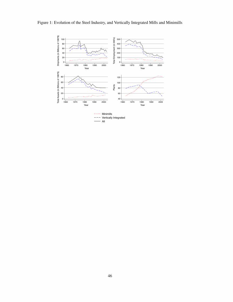
Figure 1: Evolution of the Steel Industry, and Vertically Integrated Mills and Minimills

0

20

40

60

80

100

Ship

men

ts (i

n Bi

llions

of 1

987$

)

1960 1970 1980 1990 2000Year

0

100

200

300

400

500

Tota

l Em

ploy

men

t (in

000

's)

1960 1970 1980 1990 2000Year

0

20

40

60

80

Tota

l Ass

ets

(in B

illion

s of

198

7$)

1960 1970 1980 1990 2000Year

40

60

80

100

120

Plan

ts

1960 1970 1980 1990 2000Year

0

20

40

60

80

100

Ship

men

ts (i

n Bi

llions

of 1

987$

)

1960 1970 1980 1990 2000Year

MinimillsVertically IntegratedAll

46

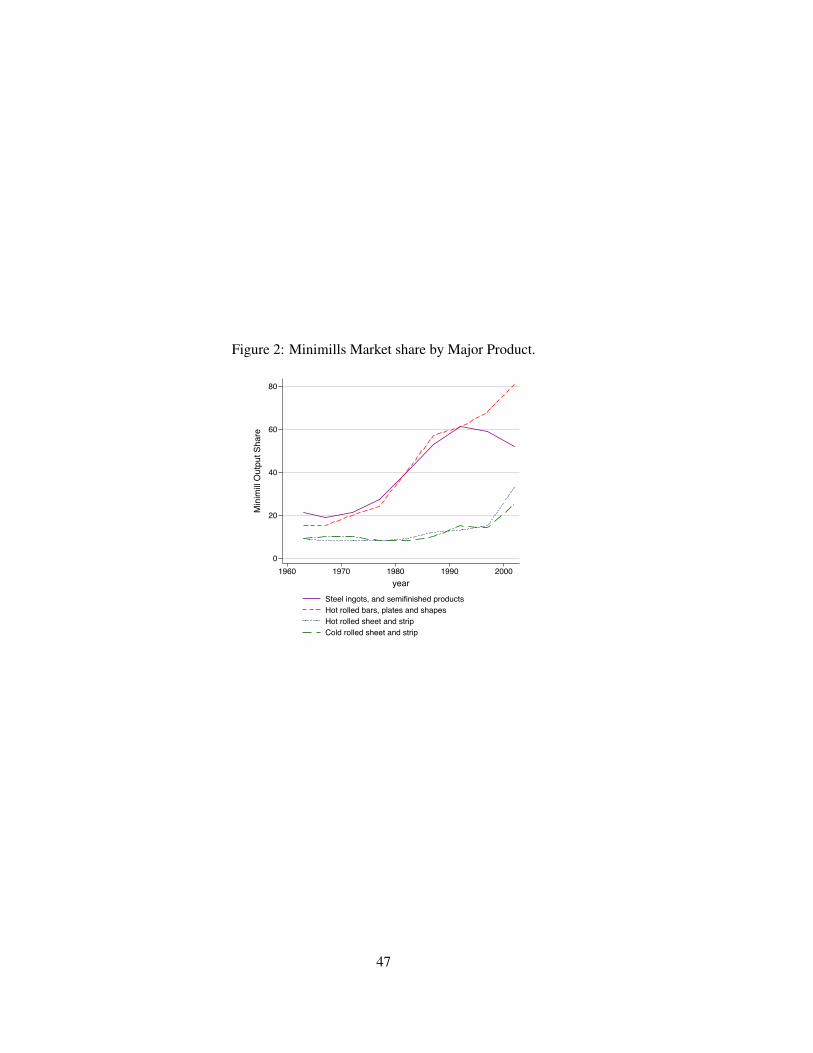
Figure 2: Minimills Market share by Major Product.

0

20

40

60

80

Min

imill

Out

put S

hare

1960 1970 1980 1990 2000year

ingotsHRBHRSCRS

0

20

40

60

80

Min

imill

Out

put S

hare

1960 1970 1980 1990 2000year

Steel ingots, and semifinished productsHot rolled bars, plates and shapesHot rolled sheet and stripCold rolled sheet and strip

47

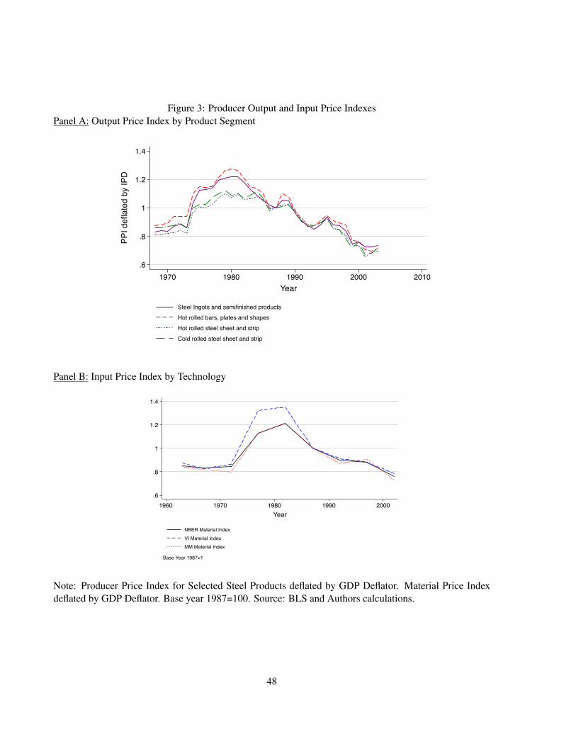
Figure 3: Producer Output and Input Price IndexesPanel A: Output Price Index by Product Segment

.6

.8

1

1.2

1.4

PPI d

eflat

ed b

y IP

D

1970 1980 1990 2000 2010Year

Steel Ingots and semifinished productsHot rolled bars, plates and shapesHot rolled steel sheet and stripCold rolled steel sheet and strip

Panel B: Input Price Index by Technology

.6

.8

1

1.2

1.4

1960 1970 1980 1990 2000Year

NBER Material IndexVI Material IndexMM Material Index

Base Year 1987=1

Note: Producer Price Index for Selected Steel Products deflated by GDP Deflator. Material Price Indexdeflated by GDP Deflator. Base year 1987=100. Source: BLS and Authors calculations.

48

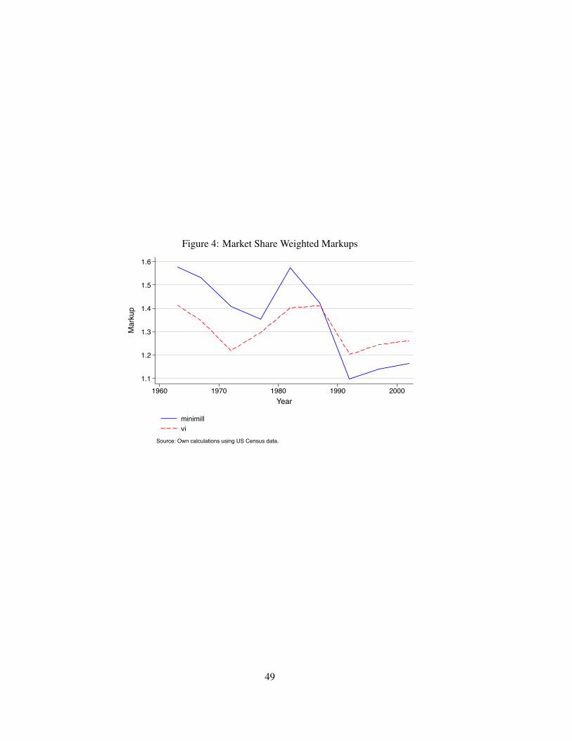
Figure 4: Market Share Weighted Markups

1.1

1.2

1.3

1.4

1.5

1.6

Mar

kup

1960 1970 1980 1990 2000Year

minimillvi

Source: Own calculations using US Census data.

49

Online Appendix for Reallocation and Technology:Evidence from the U.S. Steel Industry

Allan Collard-Wexler and Jan De LoeckerNYU and NBER, and Princeton University, NBER and CEPR

February 26, 2014

Appendix For Online Publication

A Data Appendix

A.1 Sample Selection

We pull all plants in the Census of Manufacturing, Annual Survey of Manufacturing and LongitudinalBusiness Database from 1963 to 2007 coded in either NAICS 33111 or SIC 3312 at some point in theirlives.

The Longitudinal Business Database has worse industry coding than the Census of Manufacturing,and taking its coding literally introduces a large number of non-steel mills into the sample.61 Therefore,we include a plant in the sample only if it has been coded in steel in either the CMF or the ASM.

A.2 Coding Minimills, Vertically Integrated, and Rolling Plants

A primary issue in understanding the Steel industry is how to code plants as being minimills, verticallyintegrated or rolling and processing plants. For references on the differences between minimills andvertically integrated plants and the production process for steel, see Fruehan (1998) p.1-12 and Crandall(1981) p.5-15.

The 2007, 2002 and 1997 Census of Manufacturing have a special inquiry questionnaire for thesteel industry (SI) appended to it. This questionnaire asks plants if they are considered a minimill ornot. Moreover, the SI also asks for plant hours in electric arc furnaces, blast furnaces, coke ovens, andbasic oxygen furnaces. If a plant reports plant hours in coke, blast, or basic oxygen furnace, we flagthis plant as a vertically integrated plant, since vertically integrated plants are defined by the productionprocess that first produces pig iron and slag, and then processes the result in a basic oxygen furnace. Ifa plant reports being a minimill or if it reports hours in an electric arc furnace, then we code this plantas a minimill.

Some vertically integrated plants occasionally have electric arc furnaces. Whenever a plant reporthours in an electric arc furnace and in a basic oxygen or blast furnace, we assign this plant to thevertically integrated category. The reason is that the vertically integrated section of the plant is usuallyfar bigger than the electric furnace section.

Many plants do not report hours in any steel mill department, and do not report being minimillseither. We call these plants rolling mills or processors, as they do not produce steel per se, but processsteel products. For instance, a rolling mill might use steel ingots, blooms and billets (steel shapes), androll these into steel sheet. Alternatively, a mill might take steel rods and shape them into steel screws.

For plants that were still in operation in 1997, or were built after 1997, the SI file is all we need toidentify the plant’s type. However, for plants that shut down pre-1997, we use the material and producttrailer to the Census of Manufacturing to classify them.

Minimills can be identified by their input use. Electric arc furnaces use a combination of scrap steeland direct-reduced iron as inputs. Thus, if a plant uses any direct-reduced iron, we flag this plant as aminimill. Likewise, if scrap steel represents more than 20 percent of a plant’s material use, we flag thisplant as a minimill.62

Vertically integrated plants can also be identified from their input use. If a plant uses “Coal forCoke”, this is a good indication that a plant has a blast furnace. We flag rolling mills by their use of“Steel Shapes and Forms” – steel ingots and so on that are shaped into steel products.

61In particular, the Zip Business Patterns database, that uses the same underlying source as the LBD, has a large numberof entrants coded in NAICS 33111 from 1997 to 2002 that are not steel mills.

62Basic oxygen furnaces at vertically integrated plants also can a take a small percent of scrap steel. For this reason, weflag a plant as a minimill only if scrap steel is a large part of their inputs.

1

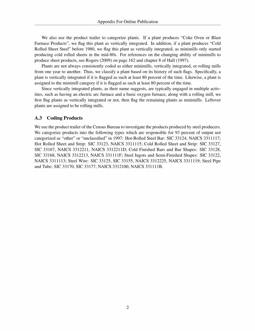
Appendix For Online Publication

We also use the product trailer to categorize plants. If a plant produces “Coke Oven or BlastFurnace Products”, we flag this plant as vertically integrated. In addition, if a plant produces “ColdRolled Sheet Steel” before 1980, we flag this plant as vertically integrated, as minimills only startedproducing cold rolled sheets in the mid-80s. For references on the changing ability of minimills toproduce sheet products, see Rogers (2009) on page 162 and chapter 8 of Hall (1997).

Plants are not always consistently coded as either minimills, vertically integrated, or rolling millsfrom one year to another. Thus, we classify a plant based on its history of such flags. Specifically, aplant is vertically integrated if it is flagged as such at least 80 percent of the time. Likewise, a plant isassigned to the minimill category if it is flagged as such at least 80 percent of the time.

Since vertically integrated plants, as their name suggests, are typically engaged in multiple activ-ities, such as having an electric arc furnace and a basic oxygen furnace, along with a rolling mill, wefirst flag plants as vertically integrated or not, then flag the remaining plants as minimills. Leftoverplants are assigned to be rolling mills.

A.3 Coding Products

We use the product trailer of the Census Bureau to investigate the products produced by steel producers.We categorize products into the following types which are responsible for 93 percent of output notcategorized as “other” or “unclassified” in 1997: Hot-Rolled Steel Bar: SIC 33124, NAICS 3311117;Hot Rolled Sheet and Strip: SIC 33123, NAICS 3311115; Cold Rolled Sheet and Strip: SIC 33127,SIC 33167, NAICS 3312211, NAICS 3312211D; Cold Finished Bars and Bar Shapes: SIC 33128,SIC 33168, NAICS 3312213, NAICS 331111F; Steel Ingots and Semi-Finished Shapes: SIC 33122,NAICS 3311113; Steel Wire: SIC 33125, SIC 33155, NAICS 3312225, NAICS 3311119; Steel Pipeand Tube: SIC 33170, SIC 33177, NAICS 3312100, NAICS 331111B.

2

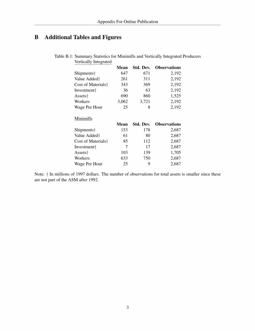
Appendix For Online Publication

B Additional Tables and Figures

Table B.1: Summary Statistics for Minimills and Vertically Integrated ProducersVertically Integrated

Mean Std. Dev. ObservationsShipments† 647 671 2,192Value Added† 261 311 2,192Cost of Materials† 343 369 2,192Investment† 36 63 2,192Assets† 690 860 1,525Workers 3,062 3,721 2,192Wage Per Hour 25 8 2,192

MinimillsMean Std. Dev. Observations

Shipments† 153 178 2,687Value Added† 61 80 2,687Cost of Materials† 85 112 2,687Investment† 7 17 2,687Assets† 103 139 1,705Workers 633 750 2,687Wage Per Hour 25 9 2,687

Note: † In millions of 1997 dollars. The number of observations for total assets is smaller since theseare not part of the ASM after 1992.

3

Appendix For Online Publication

Table B.2: Differences between Minimills and Vertically Integrated PlantsPlant-level characteristic Premium for VI Plants

All 1963 1972 1982 1992 2002

Shipments 1.44 1.60 1.60 1.46 1.32 1.02(0.08) (0.27) (0.25) (0.23) (0.23) (0.26)

Value Added 1.32 1.43 1.33 1.23 1.31 0.97(0.09) (0.30) (0.26) (0.24) (0.25) (0.28)

Assets 1.68 2.11 1.88 1.88 1.46 1.17(0.10) (0.32) (0.29) (0.27) (0.28) (0.31)

Cost of Materials 1.57 1.88 1.74 1.70 1.34 1.04(0.08) (0.28) (0.25) (0.23) (0.24) (0.26)

Employment 1.24 1.37 1.30 1.32 1.20 0.97(0.08) (0.26) (0.24) (0.22) (0.22) (0.25)

Shipment per worker 0.20 0.23 0.25 0.14 0.12 0.05(0.03) (0.10) (0.09) (0.08) (0.08) (0.10)

Value Added per worker 0.08 0.06 0.03 -0.09 0.12 0.00(0.04) (0.13) (0.11) (0.10) (0.11) (0.12)

Wage 0.06 0.04 0.07 0.14 0.00 0.07(0.01) (0.05) (0.04) (0.04) (0.04) (0.04)

Note: Estimates display the log of the ratio of the mean for VI plants over the mean for MM plants.Thus, 1.44 in the top left cell indicates that the average vertically integrated plant shipped 144 percentmore than the average minimill or, equivalently, 4.2 times more, while a coefficient of 0 indicates thatVI and MM plants have identical means. Year Controls included in each regression. There are a totalof 1499 observations in these regressions.

4

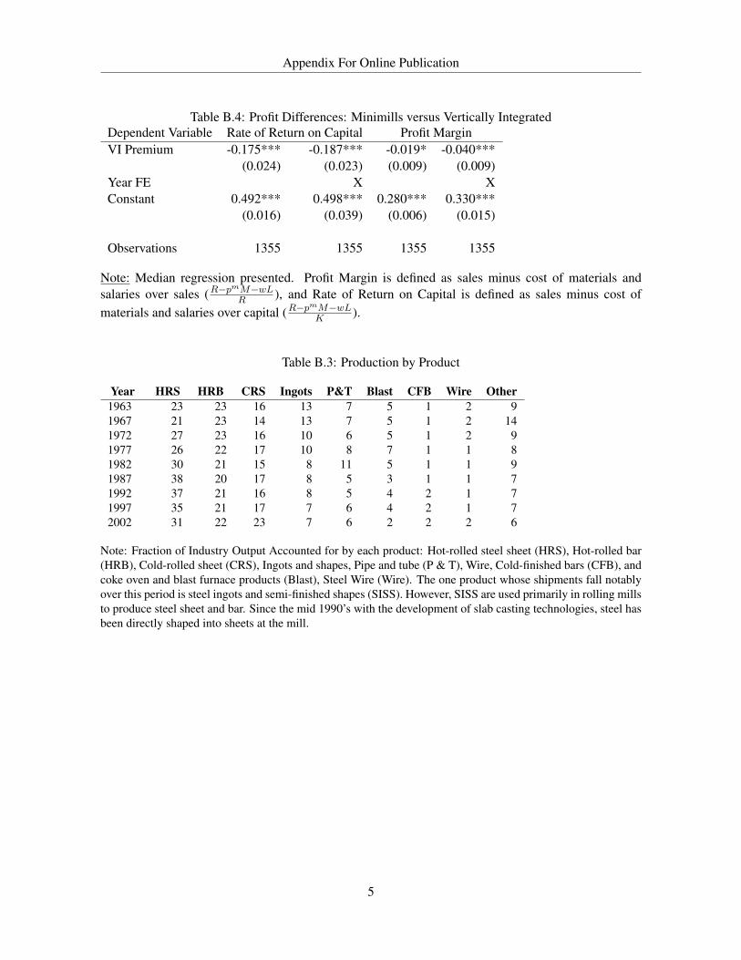
Appendix For Online Publication

Table B.4: Profit Differences: Minimills versus Vertically IntegratedDependent Variable Rate of Return on Capital Profit MarginVI Premium -0.175*** -0.187*** -0.019* -0.040***

(0.024) (0.023) (0.009) (0.009)Year FE X XConstant 0.492*** 0.498*** 0.280*** 0.330***

(0.016) (0.039) (0.006) (0.015)

Observations 1355 1355 1355 1355

Note: Median regression presented. Profit Margin is defined as sales minus cost of materials andsalaries over sales (R−p

mM−wLR ), and Rate of Return on Capital is defined as sales minus cost of

materials and salaries over capital (R−pmM−wLK ).

Table B.3: Production by Product

Year HRS HRB CRS Ingots P&T Blast CFB Wire Other1963 23 23 16 13 7 5 1 2 91967 21 23 14 13 7 5 1 2 141972 27 23 16 10 6 5 1 2 91977 26 22 17 10 8 7 1 1 81982 30 21 15 8 11 5 1 1 91987 38 20 17 8 5 3 1 1 71992 37 21 16 8 5 4 2 1 71997 35 21 17 7 6 4 2 1 72002 31 22 23 7 6 2 2 2 6

Note: Fraction of Industry Output Accounted for by each product: Hot-rolled steel sheet (HRS), Hot-rolled bar(HRB), Cold-rolled sheet (CRS), Ingots and shapes, Pipe and tube (P & T), Wire, Cold-finished bars (CFB), andcoke oven and blast furnace products (Blast), Steel Wire (Wire). The one product whose shipments fall notablyover this period is steel ingots and semi-finished shapes (SISS). However, SISS are used primarily in rolling millsto produce steel sheet and bar. Since the mid 1990’s with the development of slab casting technologies, steel hasbeen directly shaped into sheets at the mill.

5

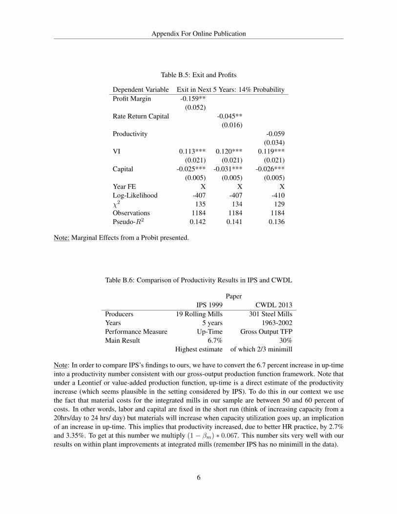
Appendix For Online Publication

Table B.5: Exit and Profits

Dependent Variable Exit in Next 5 Years: 14% ProbabilityProfit Margin -0.159**

(0.052)Rate Return Capital -0.045**

(0.016)Productivity -0.059

(0.034)VI 0.113*** 0.120*** 0.119***

(0.021) (0.021) (0.021)Capital -0.025*** -0.031*** -0.026***

(0.005) (0.005) (0.005)Year FE X X XLog-Likelihood -407 -407 -410χ2 135 134 129Observations 1184 1184 1184Pseudo-R2 0.142 0.141 0.136

Note: Marginal Effects from a Probit presented.

Table B.6: Comparison of Productivity Results in IPS and CWDL

PaperIPS 1999 CWDL 2013

Producers 19 Rolling Mills 301 Steel MillsYears 5 years 1963-2002Performance Measure Up-Time Gross Output TFPMain Result 6.7% 30%

Highest estimate of which 2/3 minimill

Note: In order to compare IPS’s findings to ours, we have to convert the 6.7 percent increase in up-timeinto a productivity number consistent with our gross-output production function framework. Note thatunder a Leontief or value-added production function, up-time is a direct estimate of the productivityincrease (which seems plausible in the setting considered by IPS). To do this in our context we usethe fact that material costs for the integrated mills in our sample are between 50 and 60 percent ofcosts. In other words, labor and capital are fixed in the short run (think of increasing capacity from a20hrs/day to 24 hrs/ day) but materials will increase when capacity utilization goes up, an implicationof an increase in up-time. This implies that productivity increased, due to better HR practice, by 2.7%and 3.35%. To get at this number we multiply (1 − βm) ∗ 0.067. This number sits very well with ourresults on within plant improvements at integrated mills (remember IPS has no minimill in the data).

6

Appendix For Online Publication

Table B.7: Industry Productivity and Foreign Competition

Specification Constant Coefficient Predicted TFP Steel Share of ActualAll 0.07 0.11 0.081 0.34

(Obs: 385) (0.03) (0.13)

Excl SIC=3674 -0.02 1.17 0.079 0.34(Obs: 384) (0.03) (0.17)

Big Sectors/Excl SIC=3674 -0.10 2.32 0.087 0.37(Obs: 80) (0.05) (0.17)

Note: We merged the NBER Manufacturing Database with the NBER U.S. Trade Database, using the 4-digit SIC87 (s) industry classification. We regress the change in aggregate productivity (∆Ω), a long dif-ference between 1972-1996, on the change in import penetration ratio. In particular we consider ∆Ωs =γ0 +γ1∆IPRs + νs. All regressions are weighted by the industry’s share in total manufacturing shipments. Bigsectors are defined as having USD 10 BLN or more in total shipments.

Table B.8: Unionization Rates

Year Steel ManufacturingUnion Membership Union Membership

1983 0.60 0.251984 0.54 0.231985 0.55 0.231986 0.56 0.221987 0.52 0.211988 0.52 0.201989 0.51 0.191990 0.49 0.201991 0.46 0.191992 0.49 0.181993 0.52 0.181994 0.45 0.171995 0.46 0.151996 0.48 0.161997 0.41 0.151998 0.40 0.151999 0.40 0.152000 0.39 0.142001 0.40 0.132002 0.36 0.13

Note: The data are directly from the CPS database and was downloaded from www.unionstats.com.

7

Appendix For Online Publication

Table B.9: Welfare effects under various demand elasticities

ε = −0.6 ε = −3.5 ε = −1

60% Fall in Prices Due to MinimillsChange CS 9.3 Billion $ 11.2 Billion $ 9.5 Billion $Share Change CS 13% 16% 13%100% Fall in Prices Due to MinimillsChange CS (All) 17 Billion $ 23 Billion $ 18 Billion $Share Change CS (All) 24 % 33 % 25 %

Note: The different elasticities of demand are based on 1) an empirical study of U.S. steel by Maasoumi et al.(2002) , 2) the implied (averaged across time and plants) elasticity of demand from our markup estimates, and3) an unit-elastic demand curve. Throughout our calculations we assume a linear demand curve. The consumersurplus is calculated as follows: R63∗ (1−∆(P02, P63)∗ (1/2+1/2∗ (1+∆(P )∗ ε)) where ∆(P02, P63) =(1/(1−∆P )) and ∆P = −0.28 ∗ λ, and λ is either 0.6 or 1, depending on the case we consider – i.e., whetherwe attribute minimills to 60 percent or 100 percent of aggregate productivity growth. All changes in CS arereported in 1997 USD.

Figure B.1: Change in Union Membership 1983-2002: Steel and the rest of manufacturing

020

4060

80

0 20 40 60 80 Member % in 1983

Member % in 2002 Member % in 1983Member % in 2002 Fitted values

Note: We plot unionization membership rates of 1983 against those of 2002. Each observation is a3-digit CIC industry, where the size of circle reflects the size in terms of employment of the industry.The red is the 45 degree line, while the yellow line indicates the line-of-best fit. The Steel Industry isrepresented by a full (green) circle. The data come from CPS (www.unionstats.com).

8

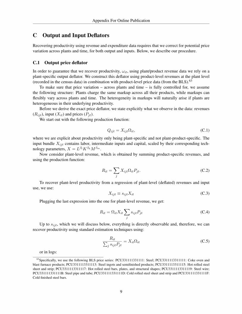
Appendix For Online Publication

C Output and Input Deflators

Recovering productivity using revenue and expenditure data requires that we correct for potential pricevariation across plants and time, for both output and inputs. Below, we describe our procedure.

C.1 Output price deflator

In order to guarantee that we recover productivity, ωit, using plant/product revenue data we rely on aplant-specific output deflator. We construct this deflator using product-level revenues at the plant level(recorded in the census data) in combination with product-level price data (from the BLS).63

To make sure that price variation – across plants and time – is fully controlled for, we assumethe following structure: Plants charge the same markup across all their products, while markups canflexibly vary across plants and time. The heterogeneity in markups will naturally arise if plants areheterogeneous in their underlying productivity.

Before we derive the exact price deflator, we state explicitly what we observe in the data: revenues(Rijt), input (Xit) and prices (Pjt).

We start out with the following production function:

Qijt = XijtΩit, (C.1)

where we are explicit about productivity only being plant-specific and not plant-product-specific. Theinput bundle Xijt contains labor, intermediate inputs and capital, scaled by their corresponding tech-nology parameters, X = LβlKβkMβm .

Now consider plant-level revenue, which is obtained by summing product-specific revenues, andusing the production function:

Rit =∑j

XijtΩitPjt. (C.2)

To recover plant-level productivity from a regression of plant-level (deflated) revenues and inputuse, we use:

Xijt ≡ sijtXit (C.3)

Plugging the last expression into the one for plant-level revenue, we get:

Rit = ΩitXit

∑j

sijtPjt (C.4)

Up to sijt, which we will discuss below, everything is directly observable and, therefore, we canrecover productivity using standard estimation techniques using:

Rit∑j sijtPjt

= XitΩit (C.5)

or in logs:63Specifically, we use the following BLS price series: PCU331111331111: Steel; PCU3311113311111: Coke oven and

blast furnace products; PCU3311113311113: Steel ingots and semifinished products; PCU3311113311115: Hot rolled steelsheet and strip; PCU3311113311117: Hot rolled steel bars, plates, and structural shapes; PCU3311113311119: Steel wire;PCU331111331111B: Steel pipe and tube; PCU331111331111D: Cold rolled steel sheet and strip and PCU331111331111F:Cold finished steel bars.

9

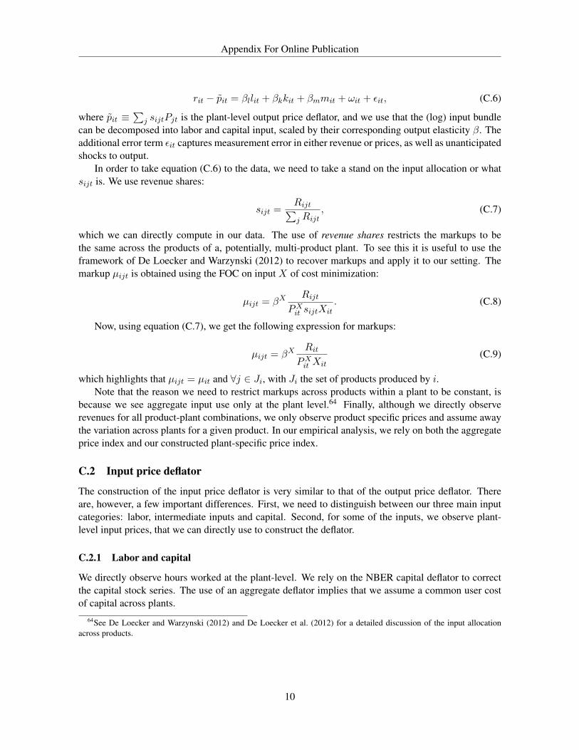
Appendix For Online Publication

rit − pit = βllit + βkkit + βmmit + ωit + εit, (C.6)

where pit ≡∑

j sijtPjt is the plant-level output price deflator, and we use that the (log) input bundlecan be decomposed into labor and capital input, scaled by their corresponding output elasticity β. Theadditional error term εit captures measurement error in either revenue or prices, as well as unanticipatedshocks to output.

In order to take equation (C.6) to the data, we need to take a stand on the input allocation or whatsijt is. We use revenue shares:

sijt =Rijt∑j Rijt

, (C.7)

which we can directly compute in our data. The use of revenue shares restricts the markups to bethe same across the products of a, potentially, multi-product plant. To see this it is useful to use theframework of De Loecker and Warzynski (2012) to recover markups and apply it to our setting. Themarkup µijt is obtained using the FOC on input X of cost minimization:

µijt = βXRijt

PXit sijtXit. (C.8)

Now, using equation (C.7), we get the following expression for markups:

µijt = βXRit

PXit Xit(C.9)

which highlights that µijt = µit and ∀j ∈ Ji, with Ji the set of products produced by i.Note that the reason we need to restrict markups across products within a plant to be constant, is

because we see aggregate input use only at the plant level.64 Finally, although we directly observerevenues for all product-plant combinations, we only observe product specific prices and assume awaythe variation across plants for a given product. In our empirical analysis, we rely on both the aggregateprice index and our constructed plant-specific price index.

C.2 Input price deflator

The construction of the input price deflator is very similar to that of the output price deflator. Thereare, however, a few important differences. First, we need to distinguish between our three main inputcategories: labor, intermediate inputs and capital. Second, for some of the inputs, we observe plant-level input prices, that we can directly use to construct the deflator.

C.2.1 Labor and capital

We directly observe hours worked at the plant-level. We rely on the NBER capital deflator to correctthe capital stock series. The use of an aggregate deflator implies that we assume a common user costof capital across plants.

64See De Loecker and Warzynski (2012) and De Loecker et al. (2012) for a detailed discussion of the input allocationacross products.

10

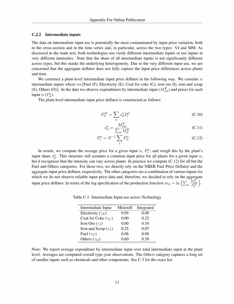
Appendix For Online Publication

C.2.2 Intermediate inputs

The data on intermediate input use is potentially the most contaminated by input price variation, bothin the cross-section and in the time series and, in particular, across the two types: VI and MM. Asdiscussed in the main text, both technologies use vastly different intermediate inputs or use inputs atvery different intensities. Note that the share of all intermediate inputs is not significantly differentacross types, but this masks the underlying heterogeneity. Due to the very different input use, we areconcerned that the aggregate deflator does not fully capture the input price differences across plantsand time.

We construct a plant-level intermediate input price deflator in the following way. We consider nintermediate inputs where n=Fuel (F), Electricity (E), Coal for coke (C), iron ore (I), iron and scrap(S), Others (O). In the data we observe expenditures by intermediate input (ME

int) and prices for eachinput n (Pnit ).

The plant-level intermediate input price deflator is constructed as follows:

PMit =∑n

snitPnt (C.10)

snit =MEint∑

nMEit

(C.11)

Pnt = N−1∑i

Pnit . (C.12)

In words, we compute the average price for a given input n, Pnt , and weigh this by the plant’sinput share snit. This structure still assumes a common input price for all plants for a given input n,but it recognizes that the intensity can vary across plants. In practice we compute (C.12) for all but theFuel and Others categories. For those two, we directly rely on the NBER Fuel Price Deflator and theaggregate input price deflator, respectively. The other categories are a combination of various inputs forwhich we do not observe reliable input price data and, therefore, we decided to rely on the aggregateinput price deflator. In terms of the log specification of the production function mit = ln

(∑nMEint

PMit

).

Table C.1: Intermediate Input use across Technology

Intermediate Input Minimill IntegratedElectricity (γE) 0.09 0.08Coal for Coke (γC) 0.00 0.22Iron Ore (γI ) 0.00 0.10Iron and Scrap (γI ) 0.25 0.07Fuel (γF ) 0.06 0.08Others (γO) 0.60 0.50

Note: We report average expenditure by intermediate input over total intermediate input at the plantlevel. Averages are computed overall type-year observations. The Others category captures a long setof smaller inputs such as chemicals and other components. See C.3 for the exact list.

11

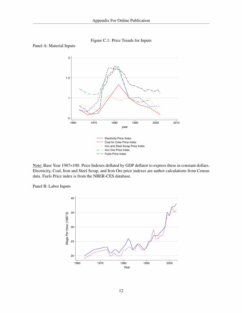
Appendix For Online Publication

Figure C.1: Price Trends for InputsPanel A: Material Inputs

.5

1

1.5

2

1960 1970 1980 1990 2000 2010year

.5

1

1.5

2

1960 1970 1980 1990 2000 2010year

Electricity Price IndexCoal for Coke Price IndexIron and Steel Scrap Price IndexIron Ore Price IndexFuels Price Index

Note: Base Year 1987=100. Price Indexes deflated by GDP deflator to express these in constant dollars.Electricity, Coal, Iron and Steel Scrap, and Iron Ore price indexes are author calculations from Censusdata. Fuels Price index is from the NBER-CES database.

Panel B: Labor Inputs

20

25

30

35

40

Wag

e Pe

r Hou

r (19

87 $

)

1960 1970 1980 1990 2000Year

12

Appendix For Online Publication

Table C.2: Input Shares: MaterialsPanel A: Minimills Input Cost Share of Materials

Year Scrap Electricity Fuels Other1963 .28 .07 .06 .601967 .26 .06 .05 .631972 .28 .08 .05 .591977 .30 .09 .07 .541982 .22 .13 .09 .551987 .30 .12 .05 .531992 .32 .10 .04 .531997 .37 .08 .04 .522002 .33 .09 .05 .52

Panel B: Vertically Integrated Input Cost Share of Materials

Year Coal for Coke Scrap Iron Ore Electricity Fuels Other1963 .10 .08 .19 .02 .08 .521967 .10 .05 .16 .02 .06 .601972 .12 .05 .16 .03 .07 .571977 .17 .06 .13 .04 .14 .471982 .14 .07 .13 .06 .14 .461987 .12 .12 .12 .06 .08 .501992 .11 .08 .18 .06 .09 .471997 .09 .09 .19 .05 .09 .492002 .08 .11 .15 .06 .10 .50

13

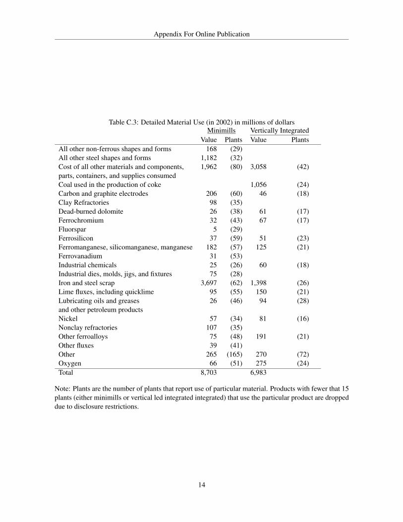
Appendix For Online Publication

Table C.3: Detailed Material Use (in 2002) in millions of dollarsMinimills Vertically Integrated

Value Plants Value PlantsAll other non-ferrous shapes and forms 168 (29)All other steel shapes and forms 1,182 (32)Cost of all other materials and components, 1,962 (80) 3,058 (42)parts, containers, and supplies consumedCoal used in the production of coke 1,056 (24)Carbon and graphite electrodes 206 (60) 46 (18)Clay Refractories 98 (35)Dead-burned dolomite 26 (38) 61 (17)Ferrochromium 32 (43) 67 (17)Fluorspar 5 (29)Ferrosilicon 37 (59) 51 (23)Ferromanganese, silicomanganese, manganese 182 (57) 125 (21)Ferrovanadium 31 (53)Industrial chemicals 25 (26) 60 (18)Industrial dies, molds, jigs, and fixtures 75 (28)Iron and steel scrap 3,697 (62) 1,398 (26)Lime fluxes, including quicklime 95 (55) 150 (21)Lubricating oils and greases 26 (46) 94 (28)and other petroleum productsNickel 57 (34) 81 (16)Nonclay refractories 107 (35)Other ferroalloys 75 (48) 191 (21)Other fluxes 39 (41)Other 265 (165) 270 (72)Oxygen 66 (51) 275 (24)Total 8,703 6,983

Note: Plants are the number of plants that report use of particular material. Products with fewer that 15plants (either minimills or vertical led integrated integrated) that use the particular product are droppeddue to disclosure restrictions.

14

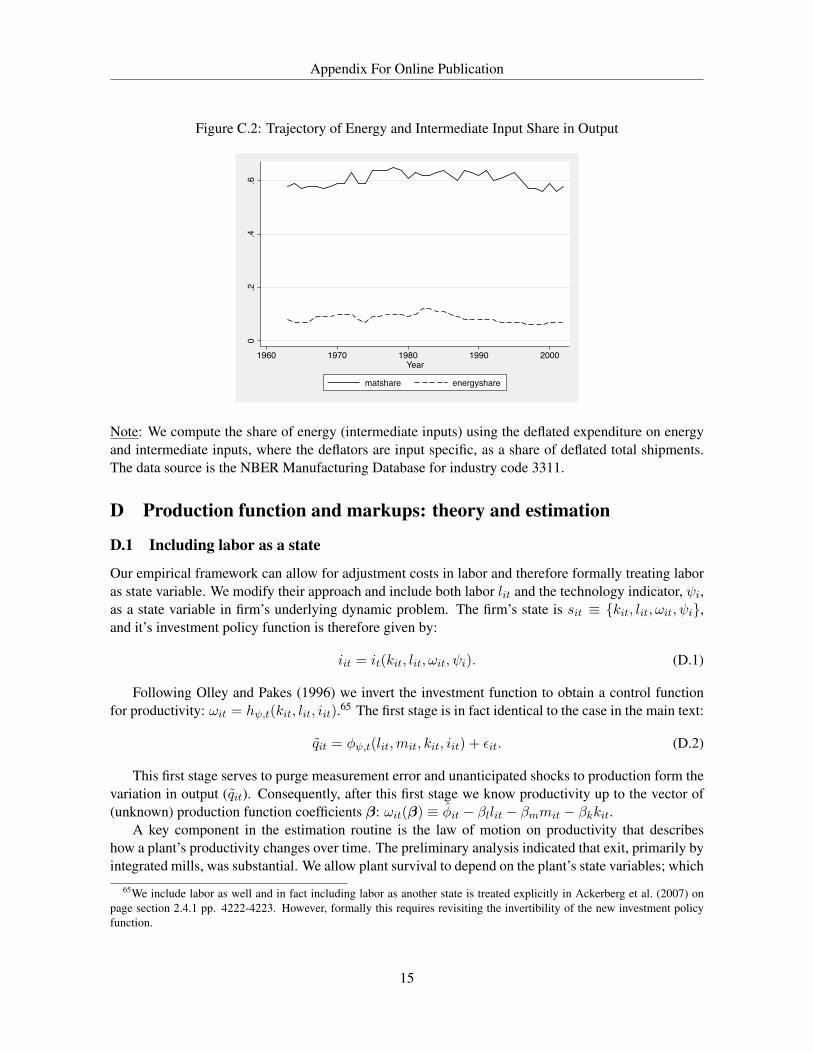
Appendix For Online Publication

Figure C.2: Trajectory of Energy and Intermediate Input Share in Output

0.2

.4.6

1960 1970 1980 1990 2000Year

matshare energyshare

Note: We compute the share of energy (intermediate inputs) using the deflated expenditure on energyand intermediate inputs, where the deflators are input specific, as a share of deflated total shipments.The data source is the NBER Manufacturing Database for industry code 3311.

D Production function and markups: theory and estimation

D.1 Including labor as a state

Our empirical framework can allow for adjustment costs in labor and therefore formally treating laboras state variable. We modify their approach and include both labor lit and the technology indicator, ψi,as a state variable in firm’s underlying dynamic problem. The firm’s state is sit ≡ kit, lit, ωit, ψi,and it’s investment policy function is therefore given by:

iit = it(kit, lit, ωit, ψi). (D.1)

Following Olley and Pakes (1996) we invert the investment function to obtain a control functionfor productivity: ωit = hψ,t(kit, lit, iit).65 The first stage is in fact identical to the case in the main text:

qit = φψ,t(lit,mit, kit, iit) + εit. (D.2)

This first stage serves to purge measurement error and unanticipated shocks to production form thevariation in output (qit). Consequently, after this first stage we know productivity up to the vector of(unknown) production function coefficients β: ωit(β) ≡ φit − βllit − βmmit − βkkit.

A key component in the estimation routine is the law of motion on productivity that describeshow a plant’s productivity changes over time. The preliminary analysis indicated that exit, primarily byintegrated mills, was substantial. We allow plant survival to depend on the plant’s state variables; which

65We include labor as well and in fact including labor as another state is treated explicitly in Ackerberg et al. (2007) onpage section 2.4.1 pp. 4222-4223. However, formally this requires revisiting the invertibility of the new investment policyfunction.

15

Appendix For Online Publication

in our case includes the technology dummy in addition to productivity, capital and labor. FollowingOlley and Pakes (1996) we rely on a nonparametric estimate of plant’s survival at time t, given theinformation set at time t− 1, It−1.

Define an indicator function χit to be equal to 1 if the firm remains active and 0 otherwise, and letωit be the productivity threshold a firm has to clear in order to survive in the market place.

The selection rule can be rewritten as:

Pr(χit = 1) = Pr [ωit ≥ ωt(lit, kit, ψi)|Iit−1]

= Pr [ωit ≥ ωt(lit, kit, ψi)|ωt(lit, kit, zit), ωit−1]

= ρt−1(ωt(lit, kit, ψi), ωit−1)

= ρt−1(lit−1, kit−1, iit−1, ψi, ωit−1)

= ρt−1(lit−1, kit−1, iit−1, iLit−1, ψi) ≡ Pit

From step 3 to 4 we use the fact that capital and labor are deterministic functions of (kt−1, lt−1, ψi, it−1, iLt−1).

We use the fact that the threshold at t is predicted using the firm’s state variables at t − 1 . As in Ol-ley and Pakes (1996), we have two different indexes of firm heterogeneity, the productivity and theproductivity cutoff point. Note that Pit = ρt−1(ωit−1, ωit) and therefore ωit = ρ−1

t−1(ωit−1,Pit).We consider the following productivity process:

ωit = gψ(ωit−1, ωit) + ξit

= gψ(ωit−1, ρ−1t−1(ωit−1,Pit)) + ξit

= gψ(ωit−1,Pit) + ξit,

(D.3)

We recover estimates of the production function coefficients, β, by forming moments on this pro-ductivity shock ξit. The identification of these coefficients relies on the rate at which inputs adjust tothese shocks. In particular, we allow both labor and capital to be dynamically chosen inputs, wherebycurrent values of capital and labor do not react to current shocks to productivity (ξit). Plants do, how-ever, adjust their intermediate input use (scrap, energy, other material inputs) to the arrival of a pro-ductivity shock ξit. While allowing for adjustment costs in capital is fairly standard in this literature,we also allow for adjustment costs in labor. One could motivate this by appealing to for example therelatively high unionization rates in the U.S. steel industry raise the potential for adjustment frictionsfor labor.

We rely on the following moments:

E

ξit(β)

litmit−1

kit

= 0. (D.4)

The production function coefficients are very similar and in particular the coefficient on labor barelychanges. So both the production function coefficients and the associated reallocation analysis leed tothe same results, both in terms of point estimates and in terms of statistical significance.

D.2 Recovering markups

We briefly discuss how we recover markups using our plant-level panel on production and prices. Ourapproach to recovering markups follows De Loecker and Warzynski (2012). In the rest of this section,we briefly review the approach. In addition to the production function we introduced before, we only

16

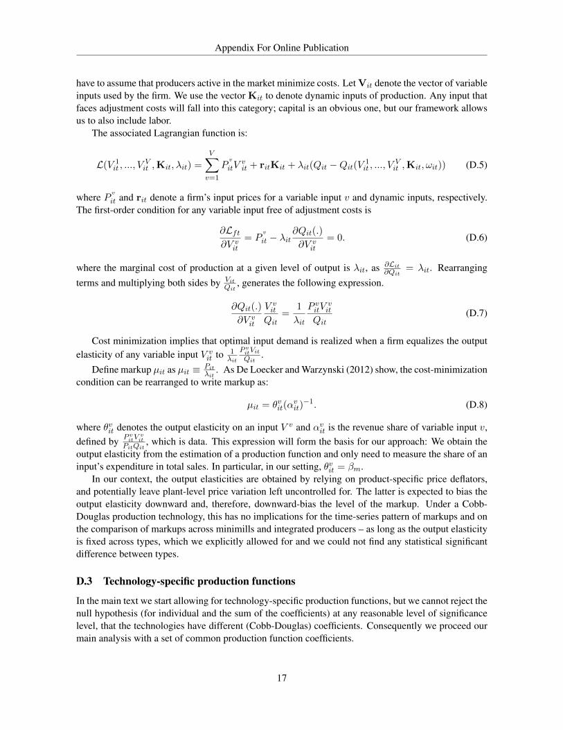
Appendix For Online Publication

have to assume that producers active in the market minimize costs. Let Vit denote the vector of variableinputs used by the firm. We use the vector Kit to denote dynamic inputs of production. Any input thatfaces adjustment costs will fall into this category; capital is an obvious one, but our framework allowsus to also include labor.

The associated Lagrangian function is:

L(V 1it , ..., V

Vit ,Kit, λit) =

V∑v=1

Pv

itVvit + ritKit + λit(Qit −Qit(V 1

it , ..., VVit ,Kit, ωit)) (D.5)

where Pv

it and rit denote a firm’s input prices for a variable input v and dynamic inputs, respectively.The first-order condition for any variable input free of adjustment costs is

∂Lft∂V v

it

= Pv

it − λit∂Qit(.)

∂V vit

= 0. (D.6)

where the marginal cost of production at a given level of output is λit, as ∂Lit∂Qit

= λit. Rearrangingterms and multiplying both sides by Vit

Qit, generates the following expression.

∂Qit(.)

∂V vit

V vit

Qit=

1

λit

P vitVvit

Qit(D.7)

Cost minimization implies that optimal input demand is realized when a firm equalizes the outputelasticity of any variable input V v

it to 1λit

P vitVitQit

.Define markup µit as µit ≡ Pit

λit. As De Loecker and Warzynski (2012) show, the cost-minimization

condition can be rearranged to write markup as:

µit = θvit(αvit)−1. (D.8)

where θvit denotes the output elasticity on an input V v and αvit is the revenue share of variable input v,defined by P vitV

vit

PitQit, which is data. This expression will form the basis for our approach: We obtain the

output elasticity from the estimation of a production function and only need to measure the share of aninput’s expenditure in total sales. In particular, in our setting, θvit = βm.

In our context, the output elasticities are obtained by relying on product-specific price deflators,and potentially leave plant-level price variation left uncontrolled for. The latter is expected to bias theoutput elasticity downward and, therefore, downward-bias the level of the markup. Under a Cobb-Douglas production technology, this has no implications for the time-series pattern of markups and onthe comparison of markups across minimills and integrated producers – as long as the output elasticityis fixed across types, which we explicitly allowed for and we could not find any statistical significantdifference between types.

D.3 Technology-specific production functions

In the main text we start allowing for technology-specific production functions, but we cannot reject thenull hypothesis (for individual and the sum of the coefficients) at any reasonable level of significancelevel, that the technologies have different (Cobb-Douglas) coefficients. Consequently we proceed ourmain analysis with a set of common production function coefficients.

17

Appendix For Online Publication

In this Appendix we that even in that setting our model actually allows for a fixed proportionproduction function for the bundle of intermediates (and we could in principal allow the same for laboralthough that a look at the data does not seem to suggest any meaningful differences), and at the sametime allows us to compare the efficiency of plants of different technologies. We turn to both the datarestrictions, and the underlying theoretical framework we rely on. The theoretical framework was infact determined by analyzing the more disaggregated intermediate input data.

D.3.1 Conceptual framework

Regardless of the differences, in any input of production, at a lower level of aggregation, our approachrests on the following production fuction:

Q = LβlKβkM(ψ)βmΩ (D.9)

where M(ψ) is our aggregate bundle of intermediate inputs which is very different across types. Giventhe specifics of both technologies in this industry we let this aggregate bundle be given by66:

M(ψ) = minγψFF, γψEE, γ

ψCC, γ

ψI I, γ

ψSS, γ

ψOO (D.10)

It is irrelevant whether we think of this production taking place inside the same plant or whether theplant can buy this aggregate intermediate inputM(ψ) from a competitive supply at price PM (just as inour Appendix on the Input price index). Ultimately what we use data on is the deflated expenditure ontotal intermediates (our m input variable). This observation is important as it allows us to rely on labor,capital and total intermediate inputs and go ahead and estimate the production function over these threewell defined variables, and makes the comparison to the literature straight forward.

Of course with ideal data on all Mn inputs, we could in turn analyze that production process. Notethat this would not benefit our analysis whatsoever: we are interested in the productivity at the plantlevel and how it differs across plants and time. The production process one level below would not haveany implications for this analysis. We just find it worthwhile reporting that both technologies get verysimilar shares on this total intermediate input bundle, about sixty eight, but this is nothing deep. Themore disaggregated intermediate input use is of course as expected very different across technologies.

An additional benefit, at least to us, is that modeling the more disaggregated intermediate inputs inthis way is that changes to individual intermediate input’s prices do not directly affect the demand forthe other intermediate inputs since they have to move in exact proportions. However, the total inputprice for the intermediate input bundle will change, as reflected by the weight of the intermediate input,and will have an effect on the total intermediate input use.

D.3.2 Disaggregation

Having said this, there are of course substantial differences between Minimills and Integrated plants interms of their input use. If we were to estimate production functions at such a level we would mostlikely find different production function coefficients. However, the data is not good enough for us toestimate a disaggregated-material production function, or the disaggregation does not seem to suggestmuch variation across types anyway (which is the case for the labor input).

66This is precisely in line with the referee’s comment on using more institutional details and knowledge in the modeling ofthe production function, given that we are only concerned with estimating the production function for one particular industry.

18

Appendix For Online Publication

For labor use at the plant-level, it turns out that salaries per worker at minimills and verticallyintegrated plants are very similar, and move in the same direction over time, as can be seen in FigureC.1 Panel B. Likewise, the skill mix of workers, say blue versus white collar, does not seem to be verydifferent between minimills and vertically integrated plants.

For materials, there is more scope for variation in input use, and differences between minimills andvertically integrated plants. Table C.1 reports the average share of an intermediate input’s expenditurein total intermediate input expenditure by plant. Given our specification for the intermediate inputbundle M(ψ), these correspond to the parameters (γ).

The results are as expected: minimills do not use any coal and iron ore, while integrated plants usemuch less scrap. It is interesting to note that both technologies are quite similar in electricity and fuelconsumption. While this table shows the average over our sample period, Tables C.2 further shows thatthese shares are extremely stable over time. We see this again as an important piece of data to supportour interpretation of the productivity differences as coming from the overall (Hicks-neutral) efficiencydifferences.

More specific to the issue of data quality at the lowest level of aggregation for intermediate inputs.Table C.3 breaks out material use by plant for 2002. You can see that even for items that all Minimillsshould use, such as Iron and Steel Scrap, a large fraction of plants do not report using any of it. Like-wise, some materials that all Vertically Integrated plants should use, such as Coal Used for Coke, wesee a large number of plants that report having a blast furnace also reporting using no Coal for Coke.We should emphasize that all of these inputs are necessary for a vertically integrated plant. So there isa substantial amount of non-response in the material trailer that prevents us from using most plants toestimates a disaggregated production function. Disregarding the issues of selection that would show upif we dropped plants that did not report using a complete list of materials, we are close enough to thedisclosure threshold at Census to make any reduction in the sample a serious impediment.67

E Deriving decompositions

We provide more details on how we derive the various decompositions introduced in the main text. Westart with the standard aggregate productivity definition:

Ωt =∑i

sitωit (E.1)

where we define:

sit =Rit∑iRit

(E.2)

Rt =∑i

Rit (E.3)

and Rit is plant-level total sales.67 This type of missing data is pervasive in the Census. In fact, the Steel Industry is perhaps the industry where collection

of these items is liable to be the most precise, and the Census of Manufacturing is also one of the better plant level datasets.So even in the “best-case” conditions, we cannot do a disaggregated materials production function analysis.

19

Appendix For Online Publication

E.1 Standard OP

Olley and Pakes show that (E.1) can be written as:

Ωit = ωt +∑i

(sit − st)(ωit − ωt)

= ωt + ΓOPt

(E.4)

with Nt the number of active plants at time t and:

ωt = N−1∑i

ωit (E.5)

st = N−1∑i

sit (E.6)

E.2 Deriving the Between covariance

We show that aggregate productivity can be decomposed in a between technology covariance compo-nent and an average type-specific productivity component, which in itself is decomposed into type-specific within and covariance terms.

Start from (E.1) and simply break up the sum into the two technology types, i.e. ψ = MM,V I:

Ωt =∑

i∈ψ=MM

sitωit +∑

i∈ψ=V I

sitωit

= st(ψ = MM)∑

i∈ψ=MM

sitst(ψ = MM)

ωit

+ st(ψ = V I)∑

i∈ψ=V I

sitst(ψ = V I)

ωit

(E.7)

The second line multiplies and divides each term by the relevant total market share of the type inthe industry, i.e. st(ψ) =

∑i∈ψ sit.

68

The last equation can now be rewritten as another weighted sum where we now sum over twogroups: minimills and integrated producers:

Ωt =∑ψ

st(ψ)Ωt(ψ) (E.8)

where

Ωt(ψ) =∑i∈ψ

sitst(ψ)

ωit =∑i∈ψ)

sit(ψ)ωit (E.9)

68The OP-decomposition relies crucially on the property that the market shares sum to one. However, if we were tosimply split the summation across the two types, we could not isolate the within covariance term. To see this, note that∑ψ Ωt(ψ) 6= Ωt, due to the fact that

∑ψ,i sit(ψ) > 1.

20

Appendix For Online Publication

The second line uses that the market share of a plant in the total industry divided by the total type-specific market share is equal to the plant’s market share in the type’s total sales (sit(ψ)). Formally:

sit(ψ) =sitst(ψ)

(E.10)

After having transformed the aggregate productivity expression into (E.8), we can rely on the sameinsight as OP and decompose aggregate productivity into a unweighted average and a covariance com-ponent. By transforming the expression using type-specific market shares we guarantee that the plantmarket shares sum to one; a necessary condition for the OP decomposition.

Applying the OP decomposition idea to (E.8) gives us:

Ωt = Ωt(ψ) +∑ψ

(st(ψ)− 0.5)(Ωt(ψ)− Ωt(ψ))

= Ωt(ψ) + ΓBt

(E.11)

E.3 Within type decompositions

Starting from equation (E.11) we simply apply the OP decomposition by type ψ and use the fact thatwe only have two technology types to obtain an expression for the average component:

Ωt(ψ) =1

2

∑ψ

(Ωt(ψ))

=1

2

∑ψ

(ωt(ψ) +∑i∈ψ

(sit(ψ)− st(ψ))(ωit − ωt(ψ)))

=1

2

∑ψ

(ωt(ψ) + ΓOPt (ψ))

(E.12)

where we denote the average market share across a given type by st(ψ) = N−1ψ

∑i∈ψ sit(ψ).

E.4 Total decomposition

To arrive at the expressions used in the main text we introduce Γt(ψ) to denote a covariance of a giventype and use superscripts B and OP to indicate whether the covariance is between or within the type,respectively. This gives us the following total decomposition of aggregate productivity:

Ωt =1

2

∑ψ

[ωt(ψ) + ΓOPt (ψ)] + ΓBt (ψ) (E.13)

If there was no entry or exit we can then directly evaluate the share of each component by trackingΩt over time. We incorporate the turnover process by relying on dynamic decompositions withina given type and can always scale the various subcomponents back to the decomposition discussedabove.

21

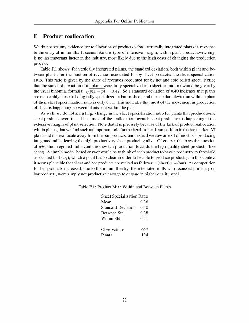
Appendix For Online Publication

F Product reallocation

We do not see any evidence for reallocation of products within vertically integrated plants in responseto the entry of minimills. It seems like this type of intensive margin, within plant product switching,is not an important factor in the industry, most likely due to the high costs of changing the productionprocess.

Table F.1 shows, for vertically integrated plants, the standard deviation, both within plant and be-tween plants, for the fraction of revenues accounted for by sheet products: the sheet specializationratio. This ratio is given by the share of revenues accounted for by hot and cold rolled sheet. Noticethat the standard deviation if all plants were fully specialized into sheet or into bar would be given bythe usual binomial formula:

√p(1− p) = 0.47. So a standard deviation of 0.40 indicates that plants

are reasonably close to being fully specialized in bar or sheet, and the standard deviation within a plantof their sheet specialization ratio is only 0.11. This indicates that most of the movement in productionof sheet is happening between plants, not within the plant.

As well, we do not see a large change in the sheet specialization ratio for plants that produce somesheet products over time. Thus, most of the reallocation towards sheet production is happening at theextensive margin of plant selection. Note that it is precisely because of the lack of product reallocationwithin plants, that we find such an important role for the head-to-head competition in the bar market. VIplants did not reallocate away from the bar products, and instead we saw an exit of most bar-producingintegrated mills, leaving the high productivity sheet producing alive. Of course, this begs the questionof why the integrated mills could not switch production towards the high quality steel products (likesheet). A simple model-based answer would be to think of each product to have a productivity thresholdassociated to it (ωj), which a plant has to clear in order to be able to produce product j. In this contextit seems plausible that sheet and bar products are ranked as follows: ω(sheet)> ω(bar). As competitionfor bar products increased, due to the minimill entry, the integrated mills who focussed primarily onbar products, were simply not productive enough to engage in higher quality steel.

Table F.1: Product Mix: Within and Between Plants

Sheet Specialization RatioMean 0.36Standard Deviation 0.40Between Std. 0.38Within Std. 0.11

Observations 657Plants 124

22