Embed Size (px)
Citation preview
Rebalancing, Conditional Value at Risk, and t-Copula
in Asset Allocation
Irvin Di Wang and Perry Xiao Zhan Zheng
Professor Emma Rasiel and Professor Aino Levonmaa, Faculty Advisors
April 19, 2010
Duke University
Durham, North Carolina
Honors Thesis submitted in partial ful�llment of the requirements for Graduation with Distinction inEconomics in Trinity College of Duke University.
Acknowledgments
We are especially grateful to our advisors, Professor Emma Rasiel and Professor Aino Levonmaa,
for their guidance, encouragement, and vision. We are also very grateful to Jing Li for inspiring this
research and for her guidance and support. We would like to thank Professor Michelle Connolly and
our classmates from Econ 198S (Fall 2009) as well for their feedback on our research, writings, and
presentations.
Abstract
Traditional asset allocation methods for modeling the tradeo� between risk and return do not
fully re�ect empirical distributions. Thus, recent research has moved away from assumptions of
normality to account for risk by looking at �fat tails� and asymmetric distributions. Other studies
have also considered multiple period frameworks to include asset rebalancing. We investigate the
use of rebalancing with fat tail distributions and optimizing with downside risk as a consideration.
Our results verify the underperformance of traditional methods in the single period framework and
also demonstrate the underperformance of traditional methods in a multiple period rebalancing
framework.
Contents
1 Introduction and Literature Review 5
2 Data and Simulations 8
2.1 Historical Data . . . . . . . . . . . . . . . . . . . . . . . . . . . . . . . . . . . . . . . . . . 82.2 Detecting and Removing Autocorrelation . . . . . . . . . . . . . . . . . . . . . . . . . . . 92.3 t-Copula Fitting . . . . . . . . . . . . . . . . . . . . . . . . . . . . . . . . . . . . . . . . . 92.4 Generating Simulations . . . . . . . . . . . . . . . . . . . . . . . . . . . . . . . . . . . . . 102.5 Summary Statistics . . . . . . . . . . . . . . . . . . . . . . . . . . . . . . . . . . . . . . . . 11
3 Methodology 12
3.1 Arithmetic and Geometric Returns . . . . . . . . . . . . . . . . . . . . . . . . . . . . . . . 123.2 Conditional Value at Risk (CVaR) . . . . . . . . . . . . . . . . . . . . . . . . . . . . . . . 133.3 Analytical Mean-Variance Optimization . . . . . . . . . . . . . . . . . . . . . . . . . . . . 133.4 Single Period Simulated Mean-CVaR Optimization with Arithmetic Returns . . . . . . . . 143.5 Single Period Simulated Mean-CVaR Optimization with Geometric Returns . . . . . . . 153.6 Multiple Period Simulated Mean-CVaR Optimization with Rebalancing and Geometric
Returns . . . . . . . . . . . . . . . . . . . . . . . . . . . . . . . . . . . . . . . . . . . . . . 15
4 Results and Discussion 16
4.1 Analytical Mean-Variance E�cient Frontiers . . . . . . . . . . . . . . . . . . . . . . . . . . 164.2 Single Period (buy and hold) Mean-CVaR . . . . . . . . . . . . . . . . . . . . . . . . . . . 174.3 Rebalancing and Geometric Mean-CVaR . . . . . . . . . . . . . . . . . . . . . . . . . . . . 184.4 Optimal Mean-CVaR E�cient Frontiers in the Mean-Variance Framework . . . . . . . . . 204.5 Comparison of the Asset Allocation Weights . . . . . . . . . . . . . . . . . . . . . . . . . . 21
5 Conclusion 22
References 25
List of Tables
1 Annual Statistics: Historical Data . . . . . . . . . . . . . . . . . . . . . . . . . . . . . . . 112 Annual Statistics: Unsmoothed Historical Data . . . . . . . . . . . . . . . . . . . . . . . . 113 Annual Statistics: t-Copula Simulation Data . . . . . . . . . . . . . . . . . . . . . . . . . 114 Historical Correlation of Monthly Returns . . . . . . . . . . . . . . . . . . . . . . . . . . . 115 t-Copula Correlation of Monthly Returns . . . . . . . . . . . . . . . . . . . . . . . . . . . 12
List of Figures
1 Normal Mean Variance E�cient Frontiers . . . . . . . . . . . . . . . . . . . . . . . . . . . 162 Single Period Arithmetic Mean-CVaR . . . . . . . . . . . . . . . . . . . . . . . . . . . . . 183 Single Period Geometric Mean-CVaR . . . . . . . . . . . . . . . . . . . . . . . . . . . . . . 194 Multiple Period Rebalancing Mean-CVaR . . . . . . . . . . . . . . . . . . . . . . . . . . . 195 All Three Mean-CVaR E�cient Frontiers . . . . . . . . . . . . . . . . . . . . . . . . . . . 206 Corresponding Mean-Variance E�cient Frontiers . . . . . . . . . . . . . . . . . . . . . . . 217 Mean Variance Weights . . . . . . . . . . . . . . . . . . . . . . . . . . . . . . . . . . . . . 218 Single Period Arithmetic Mean-CVaR Weights . . . . . . . . . . . . . . . . . . . . . . . . 219 Single Period Geometric Mean-CVaR Weights . . . . . . . . . . . . . . . . . . . . . . . . . 2210 Multiple Period Rebalancing Mean-CVaR Weights . . . . . . . . . . . . . . . . . . . . . . 22
1 Introduction and Literature Review
The tradeo� between risk and return is the fundamental principle of the investment process. Although
choosing individual investment opportunities is important, the top-down analysis of the entire investment
portfolio is crucial for maintaining and updating investment goals. The decision of how to allocate
capital across asset classes is a critical investment decision that serves as the foundation for building an
investment strategy. Traditional mean-variance asset allocation frameworks use a normal distribution
to model returns and variance as its risk measure. While these traditional methods for understanding
risk and return have come under �re in the recent �nancial turmoil, research in alternative models is
a growing and promising �eld. Recent research focuses on other risk measures for capturing downside
risk and di�erent probability distributions to account for extreme events. We are interested in building
upon the recent research in asset allocation by investigating how portfolio rebalancing can be included.
Markowitz (1952) pioneered the use of mean-variance optimization to understand the tradeo� between
risk and return for a portfolio of risky assets. Markowitz assumes asset returns are normally distributed,
providing a tractable model for the minimization of variance and the maximization of expected returns.
The analytical solution of this optimization problem is a set of portfolios along the e�cient frontier that
represents the best possible returns for each level of variance. Markowitz set the foundation for asset
allocation research and understanding the tradeo� between risk and return in a portfolio of risky assets.
In traditional mean-variance portfolio optimization frameworks, it is assumed that returns are nor-
mally distributed and joint probabilities are properly captured by the historical, linear correlation matrix.
The shortfall of this method is the thinness of the normal probability distribution's tail, implying a very
low likelihood for situations where all asset classes are falling signi�cantly in market crash scenarios.
Recent research uses a copula �t that can accommodate empirically higher probabilities of joint events
(crashes or bubbles). A copula combines marginal cumulative distribution functions (CDF) and historical
data of each asset class to create a best �t joint multivariate distribution. A Gaussian copula assumes
a multivariate normal distribution whereas a t-copula utilizes a multivariate Student's t-distribution,
allowing for fatter tails. The t-copula provides a more accurate representation of real world �nancial
markets and the probability of extreme events (Demarta and McNeil, 2004).
Sheikh and Qiao (2009) provide a real world application and veri�cation of the use of fat tail distri-
butions and CVaR as a risk measure in an asset allocation framework. It is demonstrated that a fat tail
distribution better describes the real world market environment than a normal distribution; Student's
t-copula more closely �ts the historical data, especially the extreme events, than does the normal cop-
ula. Furthermore, simulations generated from a t-copula more accurately re�ects historical data than
5
simulations generated from a normal copula. The presence of a fat tail in the t-copula allows for a more
accurate representation of extreme events for investigating downside risk.
Variance provides a mathematically simple measure of risk for asset allocation, but it is insu�cient
as a measure of downside risk. Variance symmetrically accounts for both upside risk and downside risk
since it is simply a measure of the sample's average squared deviation from the arithmetic mean. When
investment managers assess risk, they are typically more concerned with downside risk or losses and
view upside risk (which may be referred to as �excess return�) favorably. Value-at-risk (VaR) has been
incorporated as another risk measure that aims to better account for downside risk than variance. VaR
is the minimum expected loss at a certain con�dence level (typically 5%) and can be calculated from a
probability density function (PDF) of return data (either historical or simulated). However, VaR fails
to capture the extent of the possible losses beyond the speci�ed (5%) cuto�. It is possible to have two
PDF's with the same VaR (loss associated with the cuto� of 5%) but one with a fatter tail and greater
losses to the left of the speci�ed (5%) cuto�.
Conditional value-at-risk (CVaR) attempts to rectify this problem: CVaR is the expected loss given a
negative outcome that is greater than the VaR level, and it can be calculated as a weighted average of the
worst case losses (Agrawal, 2008). CVaR is a more reliable risk measure than VaR under non-normal and
non-continuous probability distributions because it is a �coherent risk measure� and is �sub-additive and
convex� (Krohmal, Palmquist, and Uryasev, 2002). This means that the CVaR of a portfolio is always
less than or equal to the sum of the CVaR of the weighted individual asset classes; furthermore, it can be
extended from continuous probability distributions to discrete scenarios, allowing for optimization using
simulations or discrete distributions and eliminating anomalous results such as multiple local minima.
Rockafellar and Uryasev (1999) demonstrate the use of CVaR in an asset allocation framework and
the ability to optimize CVaR using linear programming methods. The ability to use linear programming
stems from the way CVaR is calculated. Theoretically, CVaR is simply the average value beyond the
speci�ed cuto� (5%) calculated using the calculus of integrals. Rockafellar and Uryasev (1999) demon-
strate that the use of simulations and a summation to estimate the theoretical CVaR can be exploited
to �nd the minimum CVaR. The minimization of CVaR in most situations also provides a minimum
VaR because CVaR is always greater than VaR. Only in cases of extreme skewness does the minimum
VaR di�er greatly from the minimum CVaR. Rockafellar and Uryasev demonstrate the theoretical and
mathematical possibility of optimizing CVaR for portfolio asset allocation.
Sheikh and Qiao (2009) show how the CVaR framework is a useful way to compare normal distribu-
tions and fat-tail distributions. The optimal mean-CVaR e�cient frontier calculated using simulations
generated from a normal copula underestimates the downside risk in comparison to the optimal e�cient
6
frontier calculated using simulations generated from a t-copula. Also, the mean-variance optimization
has higher downside risk and a more concentrated asset allocation in comparison the the mean-CVaR
e�cient frontier.
So far, we have discussed methods for single period buy and hold portfolio optimization using CVaR
as a risk measure and a t-copula as a joint probability distribution. Realistically, as certain assets out-
perform others, the asset allocation changes endogenously as well. Recent research considers expanding
the optimization to incorporate multiple period rebalancing using the mean-variance framework as well
as the mean-CVaR framework.
Master (2003) o�ers a simple rebalancing strategy in the normal mean-variance framework, which
involves setting a target allocation. The investor only rebalances when the allocation deviates beyond a
set of trigger points. For instance, if the trigger point is 3% for all asset classes, then an investor only
rebalances when the weight for any asset class deviates more than 3% from the target weight. This is
also known as a tolerance band rebalancing strategy. According to Master, any rebalancing strategy
should incorporate some basic assumptions. The bene�t of rebalancing is inversely proportional to an
investor's risk preference: if an investor is risk tolerant, meaning he is willing to endure higher risk for
higher potential returns, then his tolerance band will be wider, meaning he will rebalance less often.
The key bene�t of rebalancing is to reduce the tracking error, which is how closely a portfolio follows
its target allocation benchmark. The process of rebalancing involves the movement of capital across
asset classes and incurs costs. The net bene�t of rebalancing is the di�erence between the bene�t of
rebalancing and the cost of rebalancing.
Sun (2006) extends the concepts of Master's research to incorporate dynamic programming to min-
imize the cost of rebalancing. Sun applies the idea to CAPM models, which use mean and variance as
the primary portfolio statistics of interest. The optimal strategy is to rebalance only when the expected
cost of trading is less than the expected cost of doing nothing. His conclusion is that periodic or toler-
ance band rebalancing provides suboptimal rebalanced portfolios. However, by treating the rebalancing
problem as an optimization problem and solving it using dynamic programming, Sun is able to reduce
overall costs of portfolio rebalancing and maximize returns.
Guastaroba (2009) applies rebalancing strategies to a portfolio optimization model that uses Con-
ditional Value at Risk (CVaR) as the risk measure. The model incorporates rebalancing as a set of
linear programming constraints. He introduces a decision variable to determine whether to rebalance
based on how much the portfolio allocation deviates from a predetermined quantile. Fixed and variable
transaction costs are both incorporated in the rebalancing decision. During every rebalancing period, an
investor rebalances if net portfolio return, taking into account �xed and proportional transaction costs,
7
is at least the predetermined required return. The paper then uses four in-and-out-of-sample windows to
test the model for di�erent levels of minimum required returns (0, 5%, and 10%) and di�erent quantile
measures (1%, 5%, 10% and 25%). Based on the back-testing results, he concludes that for a very
risk-averse investor the best choice is to rebalance two or three times in six months. On the other hand,
a less risk-averse investor should rebalance once or not at all.
Our research goal is to build o� of the recent advances in asset allocation research by extending
rebalancing to the mean-CVaR framework using a t-copula. We have reproduced the previous single
period mean-CVaR model with a t-copula and have shown that the normal mean variance framework
underpeforms in both the single period and rebalancing models. Furthermore, we investigated the
tradeo� between CVaR and variance and have found a small increase in variance in the optimal mean-
CVaR portfolios while obtaining a larger decrease in the downside risk (CVaR) in comparison to the
optimal mean-variance portfolios.
In section 2, we describe the indices used as benchmarks for the asset classes, the removal of autocor-
relation, and the generation of simulations using a t-copula. In section 3, we describe our methodology
and implementation of each component of the mean-CVaR framework. In section 4, we present our
results for each e�cient frontier analyses along with a discussion. Section 5 concludes.
2 Data and Simulations
2.1 Historical Data
We use the historical monthly return data of publicly available indices representing seven asset classes:
Morgan Stanley Capital International (MSCI) All World ($) for equities, Goldman Sachs Commodity
index (GSCI) for commodities, a blend of benchmarks for credit1, Barclays Capital U.S. Treasury In-
termediate for interest rate, a blend of benchmarks for in�ation sensitive2, National Association of Real
Estate Investment Trusts (NaREIT) for real estate, and Citi 3-month T-bills for cash. All benchmark
return data range from 1973 to 2009 and summary statistics are presented in Tables 1 & 4.
The three highest returning asset classes are equities, commodities, and real estate. Commodities has
the highest variance followed by real estate and equities. Equities and real estate have a particularly high
11973-1983 Barclays Intermediate Credit Index (investment grade index); 1983-1999 60% Barclays Intermediate CreditIndex, 40% Barclays US High Yield Index; 1999-2009 60% Barclays Intermediate Credit Index, 30% Barclays US HighYield Index, 10% Barclays CMBS Index
21973-1997 Bridgewater Simulated TIPS; 1997-2009 Barclays TIPS Index
8
in�ation while commodities has a low, positive correlation to those two asset classes. The lowest returning
asset class with the lowest variance is cash, while credit, interest rates, and in�ation have intermediate
returns and variances. Credit has a particularly high historical correlation with interest rates, in�ation,
and real estate; also, interest rates and in�ation are highly correlated. These return and correlation
characteristics will be evident in the simulations and impact the e�cient frontier optimizations.
2.2 Detecting and Removing Autocorrelation
In order to detect and remove autocorrelation between successive months, or single lag autocorrelation,
we follow the methods used by Sheikh and Qiao (2009). We use the Ljung-Box test to detect single lag
autocorrelation and the Fisher-Geltner-Webb methodology to unsmooth the data (remove single period
autocorrelation). We �nd and remove autocorrelation in �ve asset classes, equities, commodities, credit,
interest rates, and real estate; we do not test for autocorrelation in in�ation and cash due to their low
and consistent returns. As can be observed in Tables 1 & 2, removing autocorrelation increases the
variance without noticeably a�ecting the average return.
2.3 t-Copula Fitting
The historical return data of each individual asset class are �rst �t to independent, marginal Generalized
Pareto Distribution; this GPD �t is piecewise so that a di�erent function is �t to the lower tail and upper
tail to account for marginal distribution fat tails. Next, independent marginal CDFs are transformed
into their inverses, creating a uniform distribution over [0, 1]. The historical returns are then applied
to their respective inverse CDF's to determine a marginal probability of each return given the PDF.
Using Maximum Likelihood, a multivariate t-distribution �t is then constructed over these inverse CDF
historical probabilities to construct a t-copula that is identi�ed by a new correlation matrix and a single
degree of freedom.
The resulting t-Copula �t is centered at zero with characteristic fat tails, similar to a standard normal
distribution, and is used for generating simulations. The multivariate t probability density function is
de�ned as follows:
f(x) =Γ( v+d2 )
Γ(v2 )√
(πv)d|Σ|(1 +
(x+ µ)′Σ−1(x− µ)
v)−
v+d2 (1)
9
Γ(x) =
ˆ ∞0
tx−1e−tdt (2)
where d is the number of dimensions, v is the degrees of freedom, µ is the mean (zero, in this case), Σ is
the correlation matrix, and Γ is the gamma function as de�ned in Equation 2. The �t to the unsmoothed
historical data results in the new correlation table in Table 5 degrees of freedom of 25.25. The degrees
of freedom signi�es the extent of the fat tails. A degree of freedom of in�nite is essentially a normal
distribution; previous literature have found t-copulas with a degree of freedom of 30 to be a very close
approximation of a normal copula (Sheikh and Qiao, 2009).
2.4 Generating Simulations
In order to simulate a certain number of months into the future, we generate multiple single month
returns for all asset classes. A single month's return is simulated for all asset classes by generating
multivariate random numbers from the t-Copula �t and applying it to the following formula:
Simulated One Month Return = µ+ σ · ~x (3)
where µ is a vector of the historical monthly returns for each asset class, σ is a vector of the historical
standard deviations for each asset class, and ~x is a vector of the generated multivariate t random numbers.
We use the average historical, empirical monthly returns and historical, empirical standard deviations
of each asset class in our research for consistency and objectiveness. When simulations are drawn out
of a t-copula, the likelihood of a market crash scenario is an order of magnitude higher than that of a
Gaussian copula.
We simulate monthly returns of the seven asset classes for three years into the future using a t-
copula �t to the unsmoothed monthly return data. We run one thousand separate simulations. As
can be observed in Tables 1 & 3, the summary statistics of the t-copula simulations in comparison to
the historical data show that the simulations have average returns close to the unsmoothed historical
averages but have a wider range of returns exhibited in the higher standard deviations.
10
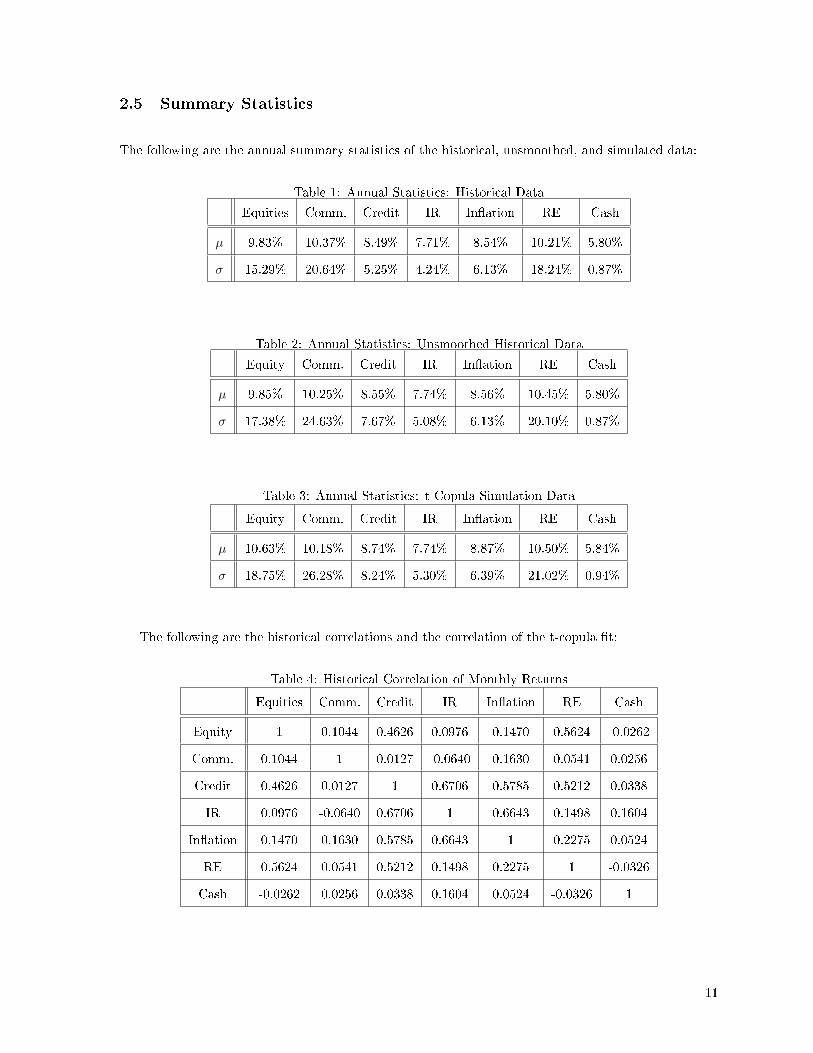
2.5 Summary Statistics
The following are the annual summary statistics of the historical, unsmoothed, and simulated data:
Table 1: Annual Statistics: Historical Data
Equities Comm. Credit IR In�ation RE Cash
µ 9.83% 10.37% 8.49% 7.71% 8.54% 10.21% 5.80%
σ 15.29% 20.64% 5.25% 4.24% 6.13% 18.24% 0.87%
Table 2: Annual Statistics: Unsmoothed Historical Data
Equity Comm. Credit IR In�ation RE Cash
µ 9.85% 10.25% 8.55% 7.74% 8.56% 10.45% 5.80%
σ 17.38% 24.63% 7.67% 5.08% 6.13% 20.10% 0.87%
Table 3: Annual Statistics: t-Copula Simulation Data
Equity Comm. Credit IR In�ation RE Cash
µ 10.63% 10.18% 8.74% 7.74% 8.87% 10.50% 5.84%
σ 18.75% 26.28% 8.24% 5.30% 6.39% 21.02% 0.94%
The following are the historical correlations and the correlation of the t-copula �t:
Table 4: Historical Correlation of Monthly Returns
Equities Comm. Credit IR In�ation RE Cash
Equity 1 0.1044 0.4626 0.0976 0.1470 0.5624 -0.0262
Comm. 0.1044 1 0.0127 -0.0640 0.1630 0.0541 0.0256
Credit 0.4626 0.0127 1 0.6706 0.5785 0.5212 0.0338
IR 0.0976 -0.0640 0.6706 1 0.6643 0.1498 0.1604
In�ation 0.1470 0.1630 0.5785 0.6643 1 0.2275 0.0524
RE 0.5624 0.0541 0.5212 0.1498 0.2275 1 -0.0326
Cash -0.0262 0.0256 0.0338 0.1604 0.0524 -0.0326 1
11
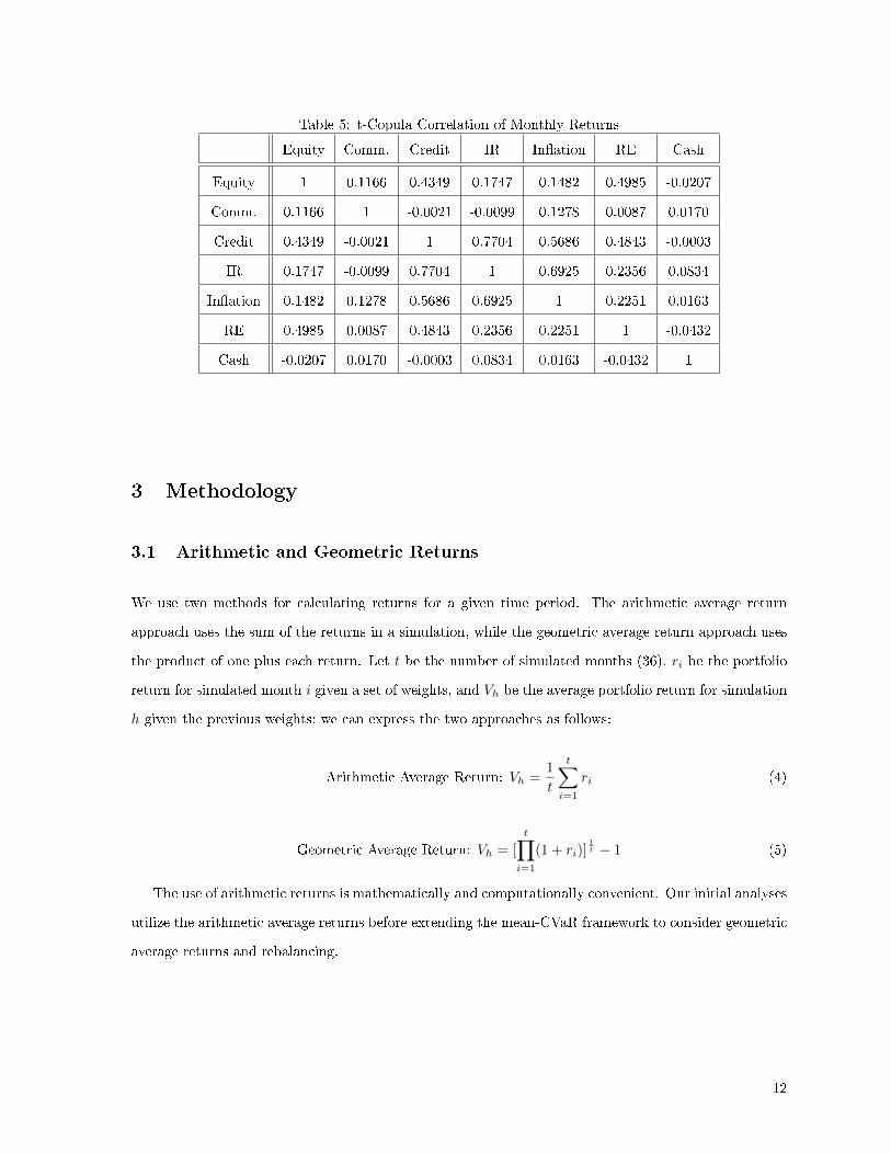
Table 5: t-Copula Correlation of Monthly Returns
Equity Comm. Credit IR In�ation RE Cash
Equity 1 0.1166 0.4349 0.1747 0.1482 0.4985 -0.0207
Comm. 0.1166 1 -0.0021 -0.0099 0.1278 0.0087 0.0170
Credit 0.4349 -0.0021 1 0.7704 0.5686 0.4843 -0.0003
IR 0.1747 -0.0099 0.7704 1 0.6925 0.2356 0.0834
In�ation 0.1482 0.1278 0.5686 0.6925 1 0.2251 0.0163
RE 0.4985 0.0087 0.4843 0.2356 0.2251 1 -0.0432
Cash -0.0207 0.0170 -0.0003 0.0834 0.0163 -0.0432 1
3 Methodology
3.1 Arithmetic and Geometric Returns
We use two methods for calculating returns for a given time period. The arithmetic average return
approach uses the sum of the returns in a simulation, while the geometric average return approach uses
the product of one plus each return. Let t be the number of simulated months (36), ri be the portfolio
return for simulated month i given a set of weights, and Vh be the average portfolio return for simulation
h given the previous weights; we can express the two approaches as follows:
Arithmetic Average Return: Vh =1
t
t∑i=1
ri (4)
Geometric Average Return: Vh = [
t∏i=1
(1 + ri)]1t − 1 (5)
The use of arithmetic returns is mathematically and computationally convenient. Our initial analyses
utilize the arithmetic average returns before extending the mean-CVaR framework to consider geometric
average returns and rebalancing.
12
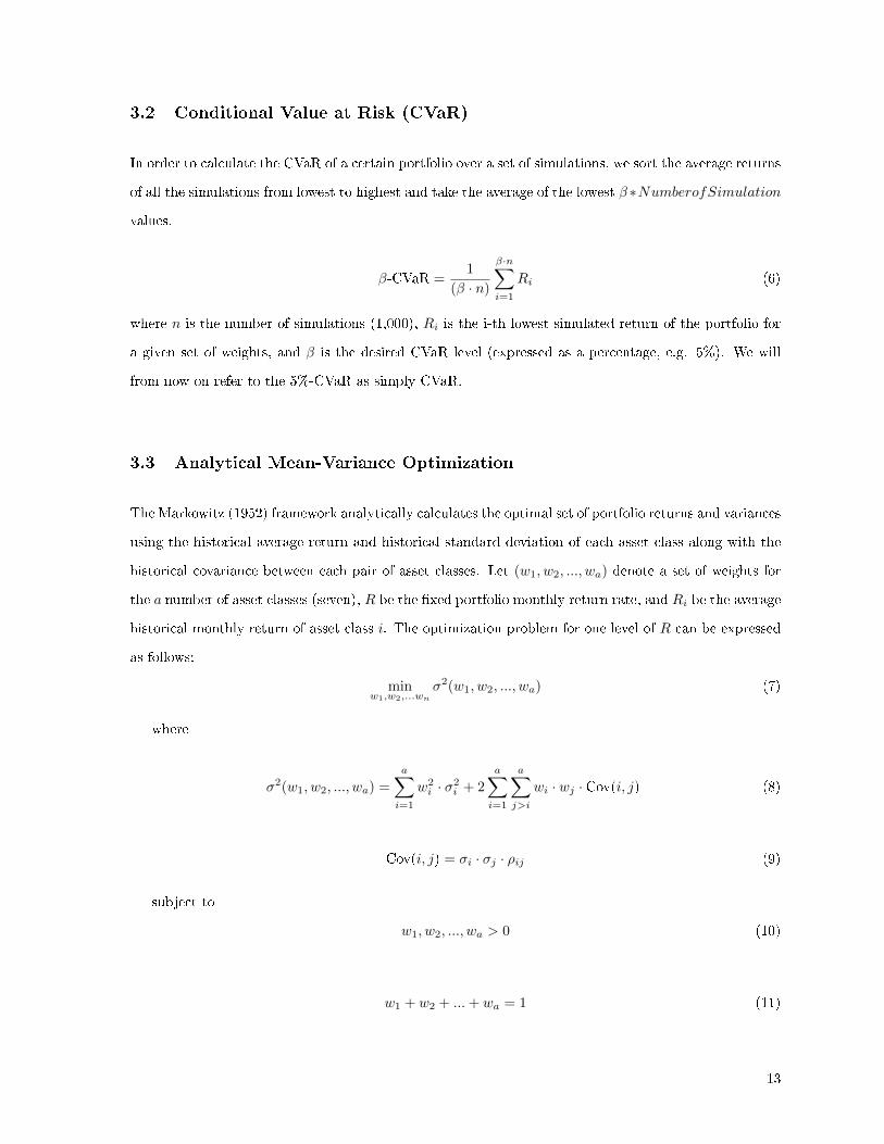
3.2 Conditional Value at Risk (CVaR)
In order to calculate the CVaR of a certain portfolio over a set of simulations, we sort the average returns
of all the simulations from lowest to highest and take the average of the lowest β ∗NumberofSimulation
values.
β-CVaR =1
(β · n)
β·n∑i=1
Ri (6)
where n is the number of simulations (1,000), Ri is the i-th lowest simulated return of the portfolio for
a given set of weights, and β is the desired CVaR level (expressed as a percentage, e.g. 5%). We will
from now on refer to the 5%-CVaR as simply CVaR.
3.3 Analytical Mean-Variance Optimization
The Markowitz (1952) framework analytically calculates the optimal set of portfolio returns and variances
using the historical average return and historical standard deviation of each asset class along with the
historical covariance between each pair of asset classes. Let (w1, w2, ..., wa) denote a set of weights for
the a number of asset classes (seven), R be the �xed portfolio monthly return rate, and Ri be the average
historical monthly return of asset class i. The optimization problem for one level of R can be expressed
as follows:
minw1,w2,...wn
σ2(w1, w2, ..., wa) (7)
where
σ2(w1, w2, ..., wa) =
a∑i=1
w2i · σ2
i + 2
a∑i=1
a∑j>i
wi · wj · Cov(i, j) (8)
Cov(i, j) = σi · σj · ρij (9)
subject to
w1, w2, ..., wa > 0 (10)
w1 + w2 + ...+ wa = 1 (11)
13
a∑i=1
wi · bi = R (12)
Our two linear constraints indicate that the weights must sum to one and be nonnegative (since no
borrowing is allowed). The optimization uses multiple levels of R between the lowest and highest single
asset class return (where the portfolio is 100% weighted in that single asset class) to determine the set
of portfolios along the e�cient frontier.
3.4 Single Period Simulated Mean-CVaR Optimization with Arithmetic Re-
turns
The single period optimization of mean-CVaR minimizes CVaR at each given level of return. The
optimization calculates the CVaR as described in Equation 6 while satisfying the condition that the
average return across all simulations is equal to the given level of return we are optimizing on. Since
this is a single period optimization, arithmetic returns are used.
Let R be the �xed portfolio monthly return rate as de�ned before and R̃ be the calculated portfolio
monthly return rate averaged across all simulations. The optimization problem for one level of R can
be expressed as follows:
minw1,w2,...wn
CVaR(w1, w2, ..., wa) (13)
subject to Equations 10, 11, and
R̃(w1, w2, ..., wa) = R (14)
where
R̃(w1, w2, ..., wn) =1
n
n∑h=1
Vh (15)
Vh =1
t
t∑i=1
ri (4′)
Since we want to optimize on a �xed return, our new constraint is that our average �nal portfolio
return R̃ across all simulations calculated with arithmetic returns must be equivalent to the given �xed
portfolio return R.
14
3.5 Single Period Simulated Mean-CVaR Optimization with Geometric Re-
turns
We adopt the geometrically calculated return approach in the this optimization. The optimization
problem for one level of R can be expressed as follows:
minw1,w2,...wn
CVaR(w1, w2, ..., wa) (16)
subject to Equations 10, 11, and 14
where Equation 15 holds and
Vh = [
t∏i=1
(1 + ri)]1t − 1 (5′)
Since we want to �x return, our new constraint is that our average �nal portfolio return R̃ across all
simulations calculated with geometric returns must be the same as the given �xed portfolio return R.
3.6 Multiple Period Simulated Mean-CVaR Optimization with Rebalancing
and Geometric Returns
The implementation is the same as in Section 3.5 with one additional feature: every 12 months, we
rebalance the portfolio to the predetermined set of weights. We calculate return of the portfolio for that
year and then redistribute the portfolio value according to the predetermined set of weights. Let ~V′s+1
be the portfolio vector after rebalancing in year s+ 1. ~V′s+1 contains the value of each asset class at the
end of year s+ 1. We have the following nonlinear programming optimization problem:
minw1,w2,...wn
CVaR(w1, w2, ..., wa) (17)
subject to Equations 10, 11, and 14
where Equation 15 holds and
Vh = V1/tf − 1 (18)
where Vf is the portfolio after the �nal rebalancing period. For each rebalancing period, the return
of the portfolio is calculated as
15
Vs+1 = Vs
p∏j=q
(1 + rj)− 1 (19)
~V′s+1 = Vs+1 · (w1, w2, .., wn) (20)
During the rebalancing period s+ 1, between time periods q and p, returns are calculated geometri-
cally. Then, at then end of the rebalancing time period s+ 1, we redistribute the value of the portfolio
according to a predetermined vector of weights to obtain a portfolio vector containing the values of each
asset class.
4 Results and Discussion
4.1 Analytical Mean-Variance E�cient Frontiers
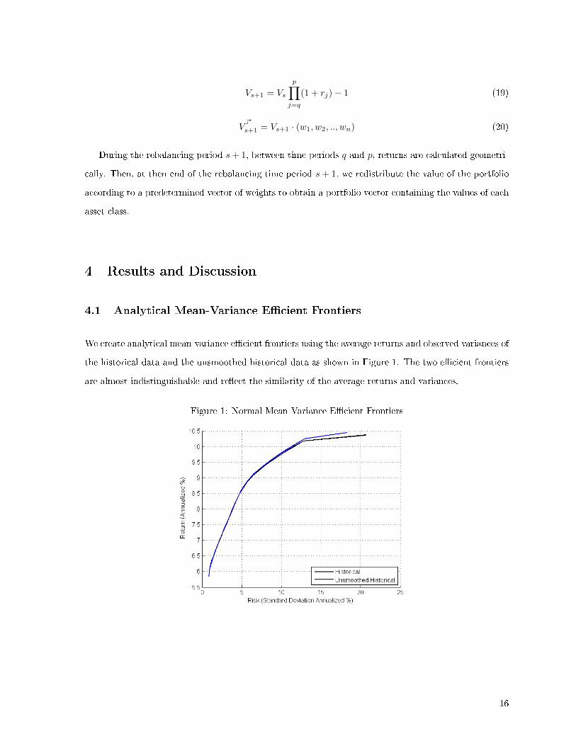
We create analytical mean-variance e�cient frontiers using the average returns and observed variances of
the historical data and the unsmoothed historical data as shown in Figure 1. The two e�cient frontiers
are almost indistinguishable and re�ect the similarity of the average returns and variances.
Figure 1: Normal Mean Variance E�cient Frontiers
16

4.2 Single Period (buy and hold) Mean-CVaR
We �rst use the resulting weights of the analytical, normal mean-variance e�cient frontiers to �nd their
corresponding portfolio CVaR's given the simulation data. We use this as a comparison to the actual
�optimal� set of portfolios in a mean-CVaR framework. The resulting e�cient frontiers are shown in
Figure 2.
The results indicate that there exists a set of portfolios that has a lower CVaR (or higher return)
than any of the analytical mean-variance portfolios. This is intuitively captured by the fact that optimal
mean-CVaR frontier lies to the upper left. The portfolios that maximize return and minimize variance
in the previous optimization (Section 4.1) have a greater CVaR than portfolios that minimize CVaR.
This suggests the mean-variance optimization does not protect against situations of extreme losses and
should not be the only consideration in asset allocation especially if preventing extreme downside risk
is a central concern.
The convergence of the e�cient frontiers at the end points is due to the fact that only a portfolio
that is 100% weighted in a single asset class can achieve the lowest possible return and the highest
possible return. The outperformance of the optimal mean-CVaR e�cient frontier in comparison to the
mean-variance e�cient frontier can be seen in the portfolios between the two endpoints.
Unlike the analytical mean-variance framework, the mean-CVaR framework allows for the risk value
to be negative. A CVaR less than zero means that the worst 5% performance is a negative loss or a small
gain. It is di�cult to use an �information ratio� or a �Sharpe ratio� since the intersection of the e�cient
frontier and the y-axis leads to arbitrarily large ratios. It is interesting to note that for an expected loss
of 0%, the optimal mean-CVaR portfolio will return almost 50 basis points more than the mean-variance
portfolio.
17
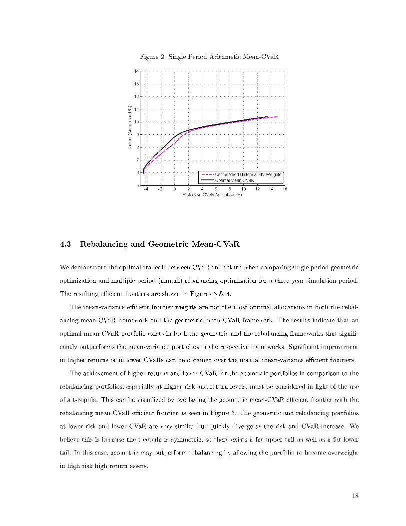
Figure 2: Single Period Arithmetic Mean-CVaR
4.3 Rebalancing and Geometric Mean-CVaR
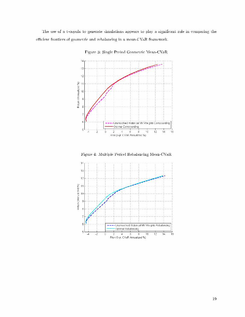
We demonstrate the optimal tradeo� between CVaR and return when comparing single period geometric
optimization and multiple period (annual) rebalancing optimization for a three year simulation period.
The resulting e�cient frontiers are shown in Figures 3 & 4.
The mean-variance e�cient frontier weights are not the most optimal allocations in both the rebal-
ancing mean-CVaR framework and the geometric mean-CVaR framework. The results indicate that an
optimal mean-CVaR portfolio exists in both the geometric and the rebalancing frameworks that signi�-
cantly outperforms the mean-variance portfolios in the respective frameworks. Signi�cant improvement
in higher returns or in lower CVaRs can be obtained over the normal mean-variance e�cient frontiers.
The achievement of higher returns and lower CVaR for the geometric portfolios in comparison to the
rebalancing portfolios, especially at higher risk and return levels, must be considered in light of the use
of a t-copula. This can be visualized by overlaying the geometric mean-CVaR e�cient frontier with the
rebalancing mean-CVaR e�cient frontier as seen in Figure 5. The geometric and rebalancing portfolios
at lower risk and lower CVaR are very similar but quickly diverge as the risk and CVaR increase. We
believe this is because the t-copula is symmetric, so there exists a fat upper tail as well as a fat lower
tail. In this case, geometric may outperform rebalancing by allowing the portfolio to become overweight
in high risk-high return assets.
18
The use of a t-copula to generate simulations appears to play a signi�cant role in comparing the
e�cient frontiers of geometric and rebalancing in a mean-CVaR framework.
Figure 3: Single Period Geometric Mean-CVaR
Figure 4: Multiple Period Rebalancing Mean-CVaR
19
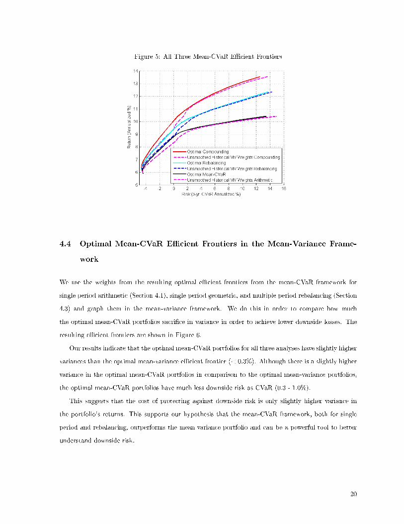
Figure 5: All Three Mean-CVaR E�cient Frontiers
4.4 Optimal Mean-CVaR E�cient Frontiers in the Mean-Variance Frame-
work
We use the weights from the resulting optimal e�cient frontiers from the mean-CVaR framework for
single period arithmetic (Section 4.1), single period geometric, and multiple period rebalancing (Section
4.3) and graph them in the mean-variance framework. We do this in order to compare how much
the optimal mean-CVaR portfolios sacri�ce in variance in order to achieve lower downside losses. The
resulting e�cient frontiers are shown in Figure 6.
Our results indicate that the optimal mean-CVaR portfolios for all three analyses have slightly higher
variances than the optimal mean-variance e�cient frontier (< 0.3%). Although there is a slightly higher
variance in the optimal mean-CVaR portfolios in comparison to the optimal mean-variance portfolios,
the optimal mean-CVaR portfolios have much less downside risk as CVaR (0.3 - 1.0%).
This suggests that the cost of protecting against downside risk is only slightly higher variance in
the portfolio's returns. This supports our hypothesis that the mean-CVaR framework, both for single
period and rebalancing, outperforms the mean-variance portfolio and can be a powerful tool to better
understand downside risk.
20

Figure 6: Corresponding Mean-Variance E�cient Frontiers
4.5 Comparison of the Asset Allocation Weights
The di�erences in the e�cient frontier performance in terms of returns and CVaR stems from the
di�erent asset allocations for each portfolio. In order to visualize the di�erences in the allocation of
capital amongst the seven asset classes, we used a 3D-ribbon graph for each of the optimal e�cient
frontiers (mean-variance and mean-CVaR) in Figures 7, 8, 9, & 10.
Figure 7: Mean Variance Weights Figure 8: Single Period Arithmetic Mean-CVaR Weights
21
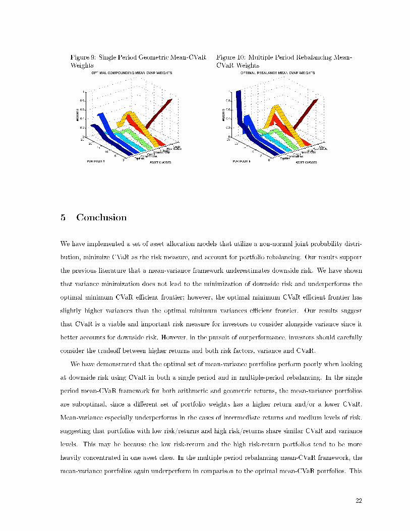
Figure 9: Single Period Geometric Mean-CVaRWeights
Figure 10: Multiple Period Rebalancing Mean-CVaR Weights
5 Conclusion
We have implemented a set of asset allocation models that utilize a non-normal joint probability distri-
bution, minimize CVaR as the risk measure, and account for portfolio rebalancing. Our results support
the previous literature that a mean-variance framework underestimates downside risk. We have shown
that variance minimization does not lead to the minimization of downside risk and underperforms the
optimal minimum CVaR e�cient frontier; however, the optimal minimum CVaR e�cient frontier has
slightly higher variances than the optimal minimum variances e�cient frontier. Our results suggest
that CVaR is a viable and important risk measure for investors to consider alongside variance since it
better accounts for downside risk. However, in the pursuit of outperformance, investors should carefully
consider the tradeo� between higher returns and both risk factors, variance and CVaR.
We have demonstrated that the optimal set of mean-variance portfolios perform poorly when looking
at downside risk using CVaR in both a single period and in multiple-period rebalancing. In the single
period mean-CVaR framework for both arithmetic and geometric returns, the mean-variance portfolios
are suboptimal, since a di�erent set of portfolio weights has a higher return and/or a lower CVaR.
Mean-variance especially underperforms in the cases of intermediate returns and medium levels of risk,
suggesting that portfolios with low risk/returns and high risk/returns share similar CVaR and variance
levels. This may be because the low risk-return and the high risk-return portfolios tend to be more
heavily concentrated in one asset class. In the multiple period rebalancing mean-CVaR framework, the
mean-variance portfolios again underperform in comparison to the optimal mean-CVaR portfolios. This
22
underperformance is also most pronounced in the medium risk-return region.
Since mean-variance inherently utilizes a normal distribution, the optimal mean-variance e�cient
frontiers do not account for scenarios of extreme joint losses. Our use of a t-copula allowed us to
properly simulate scenarios with a frequency of extreme losses similar to that observed in the historical
data. The outperformance of the optimal mean-CVaR e�cient frontier in comparison to the mean-
variance e�cient frontier is evidence that the mean-variance optimization does not account for the
extreme losses. Furthermore, the variance of the optimal mean-CVaR portfolios in each of our analyses
is marginally higher (< 0.3 %) than the variance of the corresponding optimal mean-variance portfolio.
This is smaller than the comparable gain in lower downside risk or CVaR (0.3 - 1.0 %) of the optimal
mean-CVaR e�cient frontier in comparison to the optimal mean-variance e�cient frontier. This is further
evidence that the optimal mean-CVaR analyses for both single period and rebalancing o�er pertinent
insight into the risk of extreme losses in comparison to the traditional mean-variance framework.
We have produced promising results for understanding rebalancing in the mean-CVaR framework
with non-normal joint distributions. Our rebalancing framework assumed no transaction costs and
enforced a mandatory annual redistribution of capital to the original weights. It was surprising for us
to �nd that the mean-CVaR single period geometric e�cient frontier outperforms the corresponding
rebalancing e�cient frontier. This suggests that the endogenous process of a high risk, high return asset
class becoming overweight in a single period portfolio contributes signi�cantly. It may be interesting
to investigate a dynamic optimization technique that includes a decision variable whether to rebalance;
however, we suspect that the di�culty in predicting future random returns may hinder the value of this
process. The real bene�t in a dynamic optimization process would be to bring our current rebalancing
model a step closer to real world situations with transaction costs.
Future research into the tradeo� between CVaR and variance may prove rewarding since both risk
measures could prove relevant in di�erent contexts. A three dimensional optimization that maximizes
return while minimizing variance and minimizing CVaR will produce an e�cient frontier that is a plane.
This would be an interesting framework for understanding the tradeo�s between return, variance, and
downside risk and merits future investigation. Also, future research implementing transaction costs and
a decision variable to determine when to rebalance may prove valuable as a continuation of the multiple
period rebalancing mean-CVaR framework.
The process of asset allocation is critical for understanding the overall behavior of a portfolio of risky
assets. Our research has built o� of the recent developments in applying fat-tail distributions, downside
risk measures, and rebalancing. We have developed a simple rebalancing model that incorporates a
fat-tail joint distribution in a mean-CVaR framework and have demonstrated the underperformance of
23

the traditional mean-variance framework.
24
References
Demarta, S. and McNeil, A. J. (2004). The t copula and related copulas. International Statistical Review,73(1):111�129.
Guastaroba, G. (2009). Models and simulations for portfolio rebalancing. Computational Economics,pages 237�262.
Krokhmal, P., Palmquist, J., and Uryasev, S. (2002). Portfolio optimization with conditional value-at-risk objective and constraints. Journal of Risk.
Markowitz, H. (1952). Portfolio selection. The Journal of Finance, 7(1):77�91.
Masters, S. J. (2003). Rebalancing: Establishing a consistent framework. Journal of Portfolio Manage-
ment, 29(3):52�57.
Sheikh, A. Z. and Qiao, H. (2009). Non-normality of market returns. JPMorgan White Papers.
Sun, W. A. F., Chen, L.-W., Schouwenaars, T., and Albota, M. A. (2006). Optimal rebalancing for insti-tutional portfolios: Minimizing costs using dynamic programming. Journal of Portfolio Management,32(2):33�43.
Uryasev, S. and Rockafellar, T. (2000). Optimization of conditional value-at-risk. The Journal of Risk,2(3).
25


![Infinity] Conditional Acceptance for Value (CA4V)](https://img.pdfslide.net/doc/110x75/55cfecc25503467d968befcd/infinity-conditional-acceptance-for-value-ca4v.jpg)