REBOUND: Defending Distributed Systems

Against Attacks with Bounded-Time Recovery

Neeraj GandhiUniversity of Pennsylvania

Edo RothUniversity of Pennsylvania

Brian SandlerUniversity of Pennsylvania

Andreas HaeberlenUniversity of Pennsylvania

Linh Thi Xuan PhanUniversity of Pennsylvania

Abstract

This paper shows how to use bounded-time recovery (BTR)

to defend distributed systems against non-crash faults and at-

tacks. Unlike many existing fault-tolerance techniques, BTR

does not attempt to completely mask all symptoms of a fault;

instead, it ensures that the system returns to the correct behav-

ior within a bounded amount of time. This weaker guarantee

is sufficient, e.g., for many cyber-physical systems, where

physical properties – such as inertia and thermal capacity –

prevent quick state changes and thus limit the damage that

can result from a brief period of undefined behavior.

We present an algorithm called REBOUND that can provide

BTR for the Byzantine fault model. REBOUND works by

detecting faults and then reconfiguring the system to exclude

the faulty nodes. This supports very fine-grained responses to

faults: for instance, the system can move or replace existing

tasks, or drop less critical tasks entirely to conserve resources.

REBOUND can take useful actions even when a majority of

the nodes is compromised, and it requires less redundancy

than full fault-tolerance.

ACM Reference Format:

Neeraj Gandhi, Edo Roth, Brian Sandler, Andreas Haeberlen, and Linh

Thi Xuan Phan. 2021. REBOUND: Defending Distributed Systems

Against Attacks with Bounded-Time Recovery. In Sixteenth Euro-

pean Conference on Computer Systems (EuroSys ’21), April 26–28,

2021, Online, United Kingdom. ACM, Edinburgh, Scotland, UK,

17 pages. https://doi.org/10.1145/3447786.3456257

1 Introduction

Defending distributed systems against Byzantine faults is a

well-studied problem, and many solutions are already avail-

able, such as PBFT [25] or Zyzzyva [74]. However, most of

the existing solutions have two things in common: 1) they

assume an asynchronous system, in which very little is known

about the time it takes to transmit messages or perform com-

putations, and 2) they aim for full fault tolerance – that is,

they attempt to mask all symptoms of a fault, so that the

system can continue operating as if all nodes were correct.

There are many use cases where these two assumptions

are good choices. However, they come at a price: there are

hard theoretical limits on what can be achieved in this setting

– including, for instance, the FLP impossibility result [46] and

the known lower bound of 3 f +1 replicas for asynchronous

BFT [19, 78], which tends to cause a considerable overhead.

Perhaps more importantly, the resulting guarantees do not

make any reference to time: for instance, the liveness guaran-

tee tends to promise only that something will happen “even-

tually”. In an asynchronous system, this is inevitable – there

is simply no way to provide a hard time bound.

However, we observe that there are (also) application sce-

narios where these assumptions are neither necessary nor suffi-

cient. A prime example is cyber-physical systems (CPS), such

as an industrial control system or the on-board control net-

work of a car. These systems are bona fide distributed systems

– a modern car can have hundreds of components – and attacks

on them are quite common [30, 48, 49, 75, 80, 81, 99, 119].

However, out of necessity, they 1) have been carefully en-

gineered for precise timing – with tight bounds on message

delays, careful network arbitration, and bounds on the worst-

case execution time of pretty much every single computation –

and they 2) tend to rely on embedded processors and thus tend

to be heavily resource-constrained. Because of this, asynchro-

nous BFT protocols are not necessarily an efficient choice:

they work hard to tolerate asynchrony, which CPS do not

need, and they spend considerable resources on doing so,

which most CPS cannot afford.

One way to lower the cost while preserving full fault tol-

erance would be to use a synchronous BFT protocol, such

as [2]; in this case, the lower bounds are somewhat better

(2 f +1 replicas). However, cyber-physical systems also do

not always need to completely mask all symptoms of a fault

or attack, because the physical part usually has some inertia

that limits damage at very small time scales. For instance,

suppose the attacker gains control over a burner that is under

a vat containing a volatile compound. The attacker can run

the burner continuously and eventually cause an explosion,

but lasting damage would occur only after several seconds or

minutes, not instantly. Because of this, the system can tolerate

(very) short periods in which the control system behaves arbi-

trarily, as long as the system returns to the correct behavior

within a short amount of time. The precise amount of time

depends heavily on the specific system – we have found val-

ues ranging from 500 ms for building control [93] all the way

down to 20 µs for DC/DC converters [52]. Not all of these

values may be long enough for a practical defense, but there

are definitely some where a solution seems plausible.

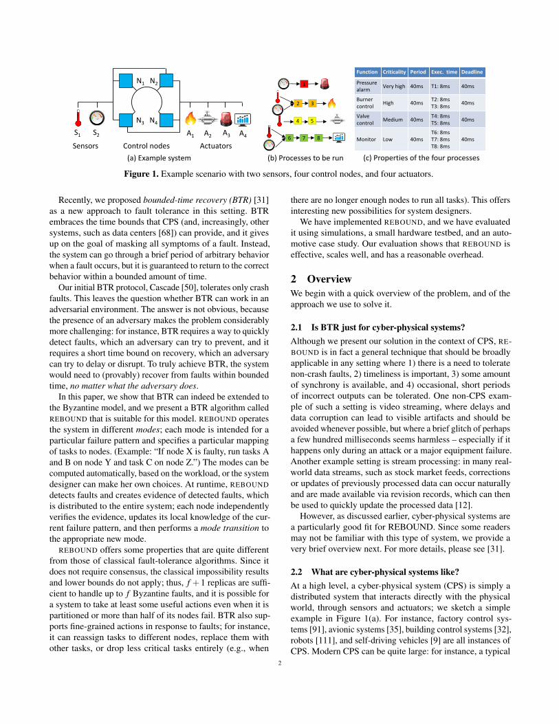
N1

S1 S2 A1

N2

N3 N4

A2A3 A4

2 3

1

6 7 8

4 5

Sensors Control nodes Actuators

Function Criticality Period Exec. time Deadline

Pressure

alarmVery high 40ms T1: 8ms 40ms

Burner

controlHigh 40ms

T2: 8ms

T3: 8ms40ms

Valve

controlMedium 40ms

T4: 8ms

T5: 8ms40ms

Monitor Low 40ms

T6: 8ms

T7: 8ms

T8: 8ms

40ms

(a) Example system (b) Processes to be run (c) Properties of the four processes

Figure 1. Example scenario with two sensors, four control nodes, and four actuators.

Recently, we proposed bounded-time recovery (BTR) [31]

as a new approach to fault tolerance in this setting. BTR

embraces the time bounds that CPS (and, increasingly, other

systems, such as data centers [68]) can provide, and it gives

up on the goal of masking all symptoms of a fault. Instead,

the system can go through a brief period of arbitrary behavior

when a fault occurs, but it is guaranteed to return to the correct

behavior within a bounded amount of time.

Our initial BTR protocol, Cascade [50], tolerates only crash

faults. This leaves the question whether BTR can work in an

adversarial environment. The answer is not obvious, because

the presence of an adversary makes the problem considerably

more challenging: for instance, BTR requires a way to quickly

detect faults, which an adversary can try to prevent, and it

requires a short time bound on recovery, which an adversary

can try to delay or disrupt. To truly achieve BTR, the system

would need to (provably) recover from faults within bounded

time, no matter what the adversary does.

In this paper, we show that BTR can indeed be extended to

the Byzantine model, and we present a BTR algorithm called

REBOUND that is suitable for this model. REBOUND operates

the system in different modes; each mode is intended for a

particular failure pattern and specifies a particular mapping

of tasks to nodes. (Example: “If node X is faulty, run tasks A

and B on node Y and task C on node Z.”) The modes can be

computed automatically, based on the workload, or the system

designer can make her own choices. At runtime, REBOUND

detects faults and creates evidence of detected faults, which

is distributed to the entire system; each node independently

verifies the evidence, updates its local knowledge of the cur-

rent failure pattern, and then performs a mode transition to

the appropriate new mode.

REBOUND offers some properties that are quite different

from those of classical fault-tolerance algorithms. Since it

does not require consensus, the classical impossibility results

and lower bounds do not apply; thus, f +1 replicas are suffi-

cient to handle up to f Byzantine faults, and it is possible for

a system to take at least some useful actions even when it is

partitioned or more than half of its nodes fail. BTR also sup-

ports fine-grained actions in response to faults; for instance,

it can reassign tasks to different nodes, replace them with

other tasks, or drop less critical tasks entirely (e.g., when

there are no longer enough nodes to run all tasks). This offers

interesting new possibilities for system designers.

We have implemented REBOUND, and we have evaluated

it using simulations, a small hardware testbed, and an auto-

motive case study. Our evaluation shows that REBOUND is

effective, scales well, and has a reasonable overhead.

2 Overview

We begin with a quick overview of the problem, and of the

approach we use to solve it.

2.1 Is BTR just for cyber-physical systems?

Although we present our solution in the context of CPS, RE-

BOUND is in fact a general technique that should be broadly

applicable in any setting where 1) there is a need to tolerate

non-crash faults, 2) timeliness is important, 3) some amount

of synchrony is available, and 4) occasional, short periods

of incorrect outputs can be tolerated. One non-CPS exam-

ple of such a setting is video streaming, where delays and

data corruption can lead to visible artifacts and should be

avoided whenever possible, but where a brief glitch of perhaps

a few hundred milliseconds seems harmless – especially if it

happens only during an attack or a major equipment failure.

Another example setting is stream processing: in many real-

world data streams, such as stock market feeds, corrections

or updates of previously processed data can occur naturally

and are made available via revision records, which can then

be used to quickly update the processed data [12].

However, as discussed earlier, cyber-physical systems are

a particularly good fit for REBOUND. Since some readers

may not be familiar with this type of system, we provide a

very brief overview next. For more details, please see [31].

2.2 What are cyber-physical systems like?

At a high level, a cyber-physical system (CPS) is simply a

distributed system that interacts directly with the physical

world, through sensors and actuators; we sketch a simple

example in Figure 1(a). For instance, factory control sys-

tems [91], avionic systems [35], building control systems [32],

robots [111], and self-driving vehicles [9] are all instances of

CPS. Modern CPS can be quite large: for instance, a typical

2

CEM SAS BCM ECM TCM SUM DRM

UEM PDM

CCM

PHM

ICM

SRS

DIM

SWM

PSM

DDM

AEM

REM

AUD

Normal ECU

ATMSUBICMMMMMP1MP2

MMS RSMSCMSRM

GSMLSM

CPM

SCM

SHM SHM

PAS

ISM

KEYHCANLCAN

MOSTLIN

Low-Power ECU

HCAN Sensors / Actuators

LCANSensors/Actuators

MOST Sensors /Actuators

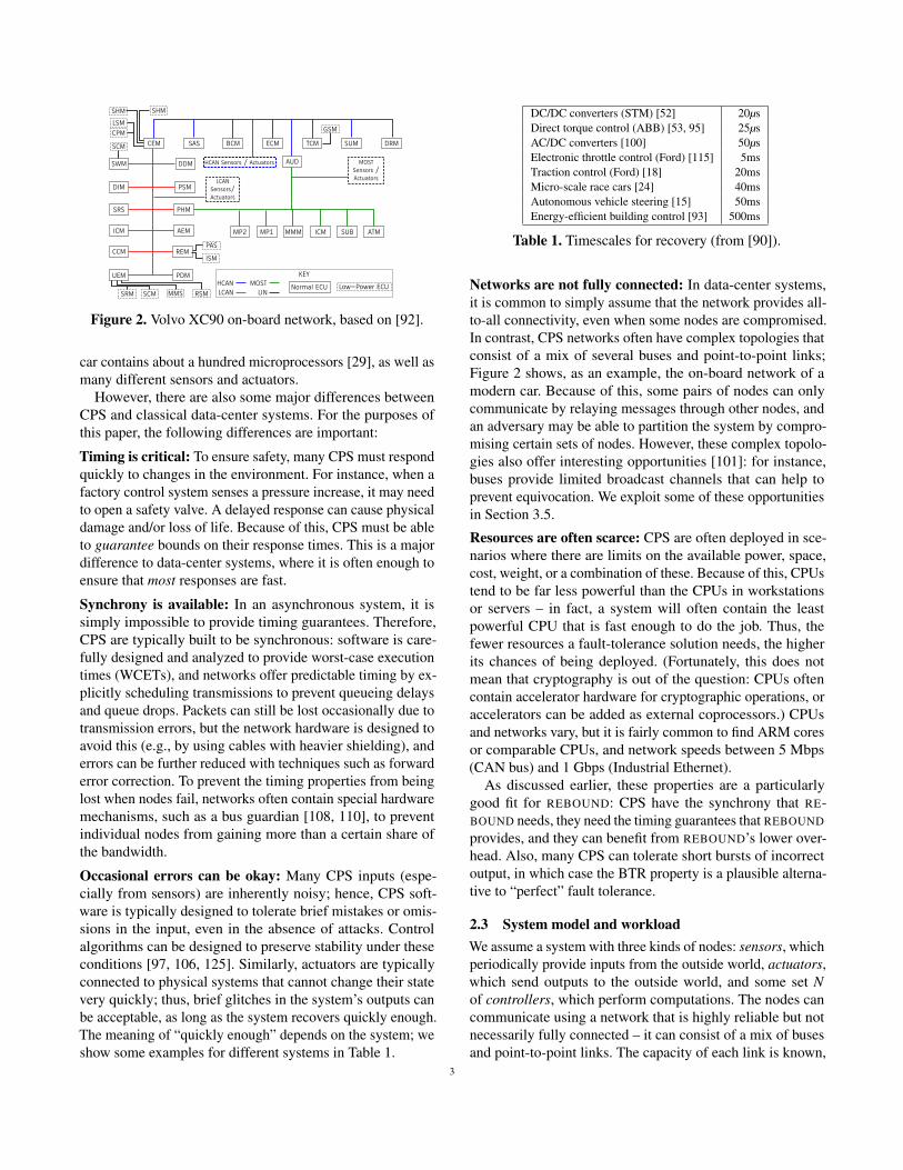
Figure 2. Volvo XC90 on-board network, based on [92].

car contains about a hundred microprocessors [29], as well as

many different sensors and actuators.

However, there are also some major differences between

CPS and classical data-center systems. For the purposes of

this paper, the following differences are important:

Timing is critical: To ensure safety, many CPS must respond

quickly to changes in the environment. For instance, when a

factory control system senses a pressure increase, it may need

to open a safety valve. A delayed response can cause physical

damage and/or loss of life. Because of this, CPS must be able

to guarantee bounds on their response times. This is a major

difference to data-center systems, where it is often enough to

ensure that most responses are fast.

Synchrony is available: In an asynchronous system, it is

simply impossible to provide timing guarantees. Therefore,

CPS are typically built to be synchronous: software is care-

fully designed and analyzed to provide worst-case execution

times (WCETs), and networks offer predictable timing by ex-

plicitly scheduling transmissions to prevent queueing delays

and queue drops. Packets can still be lost occasionally due to

transmission errors, but the network hardware is designed to

avoid this (e.g., by using cables with heavier shielding), and

errors can be further reduced with techniques such as forward

error correction. To prevent the timing properties from being

lost when nodes fail, networks often contain special hardware

mechanisms, such as a bus guardian [108, 110], to prevent

individual nodes from gaining more than a certain share of

the bandwidth.

Occasional errors can be okay: Many CPS inputs (espe-

cially from sensors) are inherently noisy; hence, CPS soft-

ware is typically designed to tolerate brief mistakes or omis-

sions in the input, even in the absence of attacks. Control

algorithms can be designed to preserve stability under these

conditions [97, 106, 125]. Similarly, actuators are typically

connected to physical systems that cannot change their state

very quickly; thus, brief glitches in the system’s outputs can

be acceptable, as long as the system recovers quickly enough.

The meaning of “quickly enough” depends on the system; we

show some examples for different systems in Table 1.

DC/DC converters (STM) [52] 20µs

Direct torque control (ABB) [53, 95] 25µs

AC/DC converters [100] 50µs

Electronic throttle control (Ford) [115] 5ms

Traction control (Ford) [18] 20ms

Micro-scale race cars [24] 40ms

Autonomous vehicle steering [15] 50ms

Energy-efficient building control [93] 500ms

Table 1. Timescales for recovery (from [90]).

Networks are not fully connected: In data-center systems,

it is common to simply assume that the network provides all-

to-all connectivity, even when some nodes are compromised.

In contrast, CPS networks often have complex topologies that

consist of a mix of several buses and point-to-point links;

Figure 2 shows, as an example, the on-board network of a

modern car. Because of this, some pairs of nodes can only

communicate by relaying messages through other nodes, and

an adversary may be able to partition the system by compro-

mising certain sets of nodes. However, these complex topolo-

gies also offer interesting opportunities [101]: for instance,

buses provide limited broadcast channels that can help to

prevent equivocation. We exploit some of these opportunities

in Section 3.5.

Resources are often scarce: CPS are often deployed in sce-

narios where there are limits on the available power, space,

cost, weight, or a combination of these. Because of this, CPUs

tend to be far less powerful than the CPUs in workstations

or servers – in fact, a system will often contain the least

powerful CPU that is fast enough to do the job. Thus, the

fewer resources a fault-tolerance solution needs, the higher

its chances of being deployed. (Fortunately, this does not

mean that cryptography is out of the question: CPUs often

contain accelerator hardware for cryptographic operations, or

accelerators can be added as external coprocessors.) CPUs

and networks vary, but it is fairly common to find ARM cores

or comparable CPUs, and network speeds between 5 Mbps

(CAN bus) and 1 Gbps (Industrial Ethernet).

As discussed earlier, these properties are a particularly

good fit for REBOUND: CPS have the synchrony that RE-

BOUND needs, they need the timing guarantees that REBOUND

provides, and they can benefit from REBOUND’s lower over-

head. Also, many CPS can tolerate short bursts of incorrect

output, in which case the BTR property is a plausible alterna-

tive to “perfect” fault tolerance.

2.3 System model and workload

We assume a system with three kinds of nodes: sensors, which

periodically provide inputs from the outside world, actuators,

which send outputs to the outside world, and some set N

of controllers, which perform computations. The nodes can

communicate using a network that is highly reliable but not

necessarily fully connected – it can consist of a mix of buses

and point-to-point links. The capacity of each link is known,

3

and we assume that, as discussed above, there is a hardware

mechanism that prevents faulty nodes from gaining more than

their share of the bandwidth. Each node has a local clock, and

clocks are synchronized to within a small time difference.

We assume a workload that consists of data flows, each

originating at some of the sensors, crossing some controllers,

and terminating at some of the actuators. This is a common

model for CPS [126]. We illustrate this model using our sim-

ple example from Figure 1(a), which is an industrial control

system from a chemical plant. This system has four data

flows, which control a burner, a valve, a monitor, and a pres-

sure alarm, based on inputs from a pressure gauge and a

temperature sensor. The sensors and actuators are attached

to a chemical reactor. Each flow can contain several tasks;

here, the flows have between one and three, which are shown

as numbered squares in Figure 1(b). Flows can be active or

inactive; each task of an active flow must be executed peri-

odically on one of the controllers. We assume that the tasks

are deterministic and that their period, worst-case execution

time, and deadline of each task are known. Figure 1(c) shows

some concrete values for our example. We also assume that,

as is common in CPS [21], each flow has been assigned a

criticality level [116], so the system can triage the flows when

it no longer has enough resources to run all of them.

2.4 Definitions and goals

We say that a controller is correct as long as its externally

observable behavior is consistent with the tasks it has been

assigned – that is, as long as it is producing the right outputs

at the right time, given the inputs it has received so far. Once a

controller is no longer correct (perhaps because it has changed,

delayed, or omitted an output, or produced an extra output),

we say that it is faulty, and we continue to consider it faulty

until it is repaired and “blessed” by an external operator. We

say that the controller fails at the moment where it transitions

from correct to faulty; of course, something could have gone

wrong inside the node before that moment, but if so, it has

not yet affected its externally observable behavior.

Our definition of a fault is consistent with the Byzantine

model [78], except that we also consider attacks on timing.

This is important for CPS: for instance, a faulty controller

could cause an explosion simply by delaying a (valid) com-

mand to shut off the burner. Note that we consider only attacks

on the controllers and not, say, an attacker who puts an ice

pack on a temperature sensor; there are orthogonal solutions,

such as attack-resilient state estimation [94], that deal with

sensors and actuators.

We have two simple goals. The first is that all active data

flows are executed on correct nodes, except for very brief

periods after a node fails. In other words, if no node fails

during interval [t −Rmax, t], then all active data flows should

be running on correct nodes at time t. We call Rmax the maxi-

mum recovery time; recall that this is a worst-case bound, and

that it depends on the system (see Table 1). Our second goal

is that the system should keep as many data flows active as it

can, though it may deactivate the least critical flows when it

no longer has enough resources to execute them all.

2.5 Threat model

We assume an adversary who is able to cause up to fmax < |N|of the compute nodes or links to fail, but no more than fconc

of them “concurrently” – that is, within the same interval

of length Rmax. It is fine to set fconc = fmax; we decided to

separate the two parameters because some costs depend only

on fconc. For instance, fconc < fmax could be used for less

powerful adversaries who are not able to synchronize faults to

within a few milliseconds, or for tolerating a combination of

adversarial and non-adversarial faults. Notice that each new

fault restarts the Rmax clock; if there is an end-to-end bound

R on the time the system can spend recovering, it would be

necessary to set Rmax := Rfconc

.

As usual in the fault-tolerance literature, we do not con-

sider fmax = |N|: if the adversary can compromise every sin-

gle node in the system, there is very little that can be done.

Physical security can prevent the adversary from tampering

with too many nodes, and software and hardware heterogene-

ity, which already exists in many CPS, can help to prevent

correlated faults, e.g., due to shared vulnerabilities. However,

we do not put any other restrictions on possible values for

fmax; it is possible to choose fmax = |N|− 1 (although this

would be expensive). This is a major difference to BFT, and,

at first glance, it seems to contradict the known impossibility

results for consensus [46]. But these do not apply here be-

cause consensus requires all decisions to be final and correct,

whereas BTR allows nodes to sometimes output incorrect

values and is thus a different, and slightly “easier”, problem.

2.6 Approach: Modes and mode changes

Our approach is to enable the system to operate in multiple

modes, which can differ in how they map tasks to nodes. At

least conceptually, there is a mode for every possible failure

scenario (KN,KL), where KN and KL represent the sets of

nodes and links that are known to have failed. For instance,

the mode ( /0, /0) is used when all nodes and links are operating

correctly, the mode (N1, /0) is used when node N1 fails, etc.

Then, at runtime, we run a protocol that detects when faulty

nodes start to deviate from their expected behavior (at a high

level, by running a few replicas and comparing their outputs),

and, whenever a new fault is detected on a node or a link,

we use the recovery period to perform a mode change to the

appropriate new mode. This will involve a brief period of

“chaos”, as nodes transition from one mode to another, but, as

long as the transition is complete before the recovery period

ends, we can still maintain the BTR guarantee.

As an illustration, Figure 3 shows a few possible modes and

mode transitions for the system in Figure 1, with fconc = 1

and fmax = 3. The mode on the left is used when all nodes

4

3

1

2 3

4

5

6

7

8

1

4

2

6

3

8

5

7

1

2 3

4

1

4

2

55

3

2 3

1

3 2

1

32

1

N2

fails

N1:

N3:

N4:

N1

fails N4

fails

N1

N2

N4

N3

N1

N2

N4

N3

N1

N2

N4

N3

N1

N2

N4

N3

6 3

6 5

8 7

N3:

N4: 5 2 1

5 4 3

1 1

N3: 3

Figure 3. A few mode transitions for the system from Figure 1, with fconc = 1 and fmax = 3. The figure shows which of the

tasks from are scheduled on which node; task copies are shown in gray. Each node can run up to four tasks or task copies.

and links are operating normally; notice that each task has one

replica, which is shown in gray. When N2 fails, the system

responds by moving task τ5 to N3 and by reconfiguring some

of the replicas; additionally, since the system no longer has

enough nodes to run the entire workload, the least critical data

flow (monitoring, shown in green) is dropped. If a second

node (N1) fails later, τ1 is moved, and the valve control task is

also dropped, but the two most critical data flows still survive.

2.7 Requirements

Next, we state the four properties we need to make this ap-

proach work. (In an extended version of this paper [51, §A],

we formally prove that REBOUND has these properties.)

Requirement 1 (Completeness). For each observable fault,

at least one faulty node or link is detected by at least one

correct node.

By “observable fault”, we mean a fault that directly or in-

directly affects at least one correct node. This restriction is

necessary to rule out faults that have no visible effects at all,

such as an unused bit flipping in a node’s memory, or two

faulty nodes whispering evil messages over a direct link be-

tween them but otherwise acting correctly. Please see [60] for

a formal definition.

Next, we add a notion of time; “eventual” detection is

not enough because, in our scenario, the adversary can win

simply by delaying the detection process long enough, e.g., by

distracting the other nodes with enormous garbage messages.

Thus, we add the following requirement:

Requirement 2 (Bounded-time detection). If an observable

fault occurs at time t, it must be detected by time t +Tdet,max.

Once a node has detected a fault, it must trigger a mode transi-

tion. However, most faults are not directly visible to all nodes

– for instance, a malicious message would only be directly

visible to the node that receives it. If we allowed nodes to

simply report faults to other nodes without further evidence,

a compromised node could abuse this mechanism to report

fabricated faults, or to sow confusion by triggering transitions

to random modes. To avoid this, we add the following:

Requirement 3 (Accuracy). If a node or link is not faulty,

no correct node will consider it to be faulty.

We accomplish this by having the node that first detects the

fault generate evidence of the fault, by distributing any such

evidence across the system, and by requiring nodes to verify

the evidence before they “believe” a new report of a fault that

they did not directly observe. The verification can be done

independently by each node and does not require consensus.

How should the system transition to a new mode? The

natural approach would be to appoint a single coordinator

node, or a group of nodes that agrees on which mode to use.

However, it is critical that we avoid both: the former because

it would create a single point of failure, and the latter because

of the known impossibility results [19, 46, 78]. Fortunately, in

our case, it is sufficient to simply flood the evidence through

the system: each node can verify it independently and then

locally transition to the new mode, without coordinating with

other nodes. The correct nodes will collectively transition

to the same mode – albeit in an unsynchronized, somewhat

messy way – as long as we can ensure that they all receive

the same evidence within a sufficiently short amount of time.

This last point creates a final complication: since we did

not assume all-to-all connectivity, we must consider the pos-

sibility that the faulty nodes can partition the network or se-

lectively refuse to forward certain messages to certain nodes.

Thus, we cannot hope to achieve global consistency, much

less within bounded time. However, a slightly weaker prop-

erty is sufficient for our purposes:

Requirement 4 (Bounded-time stabilization). If a correct

node i has valid evidence e, then, within bounded time Tstab,max,

each correct node j will either 1) receive e, or 2) conclude

that i is unreachable.

Thus, if the adversary does manage to partition the system,

each partition will at least be aware of its own extent, and

can make local decisions independently. During a partition, it

will not always be possible to mask all the symptoms of the

fault – for instance, if the sensors and actuators for some data

flows end up in different partitions, such flows can obviously

not continue. However, a system can take other actions in

response, such as scheduling new or different tasks in the

partitions. For instance, in Figure 1, a partition that contains

the burner but not the temperature sensor could schedule a

new task that shuts off the burner, and a partition that contains

the warning light but not the pressure gauge could schedule a

task that activates the light to get the operator’s attention.

5

Collectively, the four requirements are sufficient for BTR:

If it can take a node up to Tswitch,max to switch to another

mode, and Tdet,max +Tstab,max +Tswitch,max < Rmax, each ob-

servable fault will, within bounded time Rmax, cause all cor-

rect nodes to transition to a new mode, and the mode will be

consistent among the correct nodes in each partition.

3 The REBOUND algorithm

We now present REBOUND, an algorithm that meets these four

requirements. REBOUND relies on standard cryptographic as-

sumptions: it assumes that each node i has a public/private

keypair (πi,σi), that each node knows the public key of all

other nodes, and that there is a cryptographic hash function

H. REBOUND proceeds in discrete, numbered rounds, which

could, e.g., be the periods of the underlying workload. RE-

BOUND guarantees a bound on the number of rounds it can

take to detect a fault; thus, shorter rounds result in a lower

detection bound Tdet,max.

3.1 Roadmap

Existing fault-tolerance protocols typically assume that the

network is fully connected and that, at least logically, any pair

of nodes can always communicate. For REBOUND, we want to

avoid this assumption: many CPS use a mix of different buses

and links, and messages can often reach their destination only

if they are forwarded by some of the nodes, which a faulty

node may not always do.

To avoid a circular dependency between fault detection

and communication, REBOUND consists of two layers: a for-

warding layer and an auditing layer. The forwarding layer

(Section 3.3–3.4), has the following four functions. 1) It ac-

cepts, for each mode m, a set of data paths PATH(m) between

nodes that should exist in that mode. In each round, it picks

up a data packet at the source of each path and transports it to

the corresponding sink. 2) It accepts and further distributes

evidence to all correct nodes in the sender’s partition. 3) It

detects when nodes fail to perform the first two functions

correctly, and generates evidence of such faults, which it also

distributes. And 4) it selects the local mode on the node it is

running on based on the available evidence. We also describe

a number of optimizations (Section 3.5–3.6) that substantially

reduce the cost of the forwarding-layer algorithm.

The auditing layer (Section 3.7–3.8) accepts 1) a set of data

flows, and 2) a schedule for each mode m (Section 3.9) that

maps the tasks in each flow, as well as fconc copies of each

task, to specific nodes. Using the data flows and schedules,

the auditing layer gives two kinds of paths to the forward-

ing layer: a) paths that connect tasks to their upstream and

downstream neighbors; and b) “internal” paths that connect

tasks to their copies and are used for application-level fault

detection. The data flows, schedules, and path representations

are computed offline. At runtime, the auditing layer is respon-

sible for verifying that, given a set of inputs at a particular

time and previous state, the produced output is correct. If

verification fails, this is evidence of a fault that is passed to

the forwarding layer for distribution.

3.2 Generating evidence

There are two ways a node can fail: it can either send a bad

message (commission fault) or fail to send, at the correct

time, a good message it was expected to send (omission fault).

Since we need all the nodes to make a mode transition in

response to a given failure, but each commission or omission

will be visible to only some of the nodes, we cannot avoid

having the nodes exchange information about what they each

have seen. However, faulty nodes can tell lies, and since we

need accuracy, a correct node A must never simply “believe”

another node B that a third node C has said or done anything –

it must always have some concrete evidence.

Since messages are signed, evidence of commission faults

is easy: if a controller produces a bad output, that output and

the corresponding inputs constitute a proof of misbehavior

(PoM), which can be verified by other nodes and can thus

serve as evidence. But what about omission faults? Since we

consider a synchronous environment, a node can always tell

when it should expect a message to arrive.1 But in general, an

omission fault is visible only to the recipient – how would a

node prove to others that it has not received a given message?

Our approach is to simply allow both endpoints to issue a link

failure declaration (LFD), which is a message σi(LFD(i, j))that says that i and j can no longer properly communicate. A

single LFD does not attribute the failure specifically to i or

j, but this is also not necessary – since the link is clearly not

working, it should no longer be used, and a mode transition

may be necessary to redirect its flows.

Notice that we can sometimes infer node faults from mul-

tiple LFDs. Suppose, for instance, that fmax = 1 and a node

A issues LFDs for two links (A,B) and (A,C). This means

that both A,B and A,C must contain at least one faulty

node. But if fmax = 1, B and C cannot both be faulty, so the

only possible explanation is that A has failed. In general, we

can always map a mode (KN,KL) with |KN|+ |KL|> fmax

to another with |KN|+ |KL| ≤ fmax, by replacing some link

faults with node faults. (If i ∈ KL, we implicitly consider all

of i’s links to be faulty, and we do not include them in KL.)

3.3 Evidence distribution

As a first approximation, REBOUND’s forwarding layer dis-

tributes evidence of node or link faults by flooding it through

the entire system: in each round, each node i sends all of its

evidence Ei to each of its neighbors, and it verifies and stores

any new evidence it receives from them. However, this is not

1The network itself almost never loses packets. Everything is scheduled, so

there is no loss due to congestion, which leaves only link-layer loss. In our

testbed, we were able to send 109 packets without seeing a single loss.

6

1: var HBTi = /0 ▷ Heartbeats remembered by node i

2: var MSGi = /0 ▷ Messages seen by node i

3: var POMi = /0 ▷ Proofs of misbehavior seen by node i

4:

5: /* Invoked if node i receives a message m from node j in round r */

6: function RECEIVE(i, j,r,H,M)

7: if !IS-PLAUSIBLE(H,M) then return

8: if M = COMPUTE-MESSAGES( j, i,r−1,H,MSGi ∪M) then

9: HBTi = HBTi

⋃H

10: MSGi = MSGi

⋃M

11: for each σn(n,r,E) ∈ H : HBTi.CONTAINSHEARTBEAT(n,r) do

12: h = HBTi.GETHEARTBEAT(n,r)13: if σn(n,r,E) = h then

14: POMi = POMi

⋃σi(POM(n,σn(n,r,e),h)

15: /* Invoked after node i has received all messages in round r */

16: function FINISH-ROUND(i,r)

17: Hnew = COMPUTE-HEARTBEAT(i,r,HBTi,MSGi, /0)18: HBTi = HBTi

⋃σi(Hnew)

19: for p ∈ PATH(HBTi.EVIDENCE): p = (i, . . .) do

20: MSGi = MSGi

⋃GENERATE-MESSAGE(p,r)

21: for k ∈ NODES: (i,k) ∈ EDGES do

22: M = COMPUTE-MESSAGES(i,k,r,HBTi,MSGi)23: if LFD(i,k), POM(k)

⋂HBTi.EVIDENCE = /0 then

24: SEND(k,(HBTi,M))

25: function COMPUTE-HEARTBEAT(n,r,H,Enew)

26: if ((r > 0)∧ !H.CONTAINSHEARTBEAT(n,r−1)) then return ⊥

27: E = (r == 0)? /0 : H.GETHEARTBEAT(n,r−1).EVIDENCE

28: E = E⋃

Enew

29: for (k : (k,n)∈EDGES ∧ LFD(k,n) ∈ E) do

30: if H.CONTAINSHEARTBEAT(k,r−1) then

31: h = H.GETHEARTBEAT(k,r−1)

32: Enew,k = LFD(x,y) ∈ h |x = k ∨ y = k33: h′ = COMPUTE-HEARTBEAT(k,r−1,H,Enew,k)34: if (h = h′) then E = E

⋃h.EVIDENCE

35: else E = E⋃LFD(k,n)

36: else E = E⋃LFD(k,n)

37: return (n,r,E)

38: function COMPUTE-MESSAGES(nfrom,nto,r,H,M)

39: E = H.GETHEARTBEAT(nfrom,r).EVIDENCE

40: M′ = /0

41: for (k : (k,nfrom)∈EDGES ∧ LFD(k,nfrom) ∈ E) do

42: M′ = M′ ⋃COMPUTE-MESSAGES(k,nfrom,r−1,H,M)

43: M′=m∈M′|m.PATH ∈ PATH(E)∧ (nfrom,nto) ∈ m.PATH

44: for p ∈ PATH(E): p = (nfrom, . . .) do

45: if !M.CONTAINSMESSAGE(p,r) then return ⊥

46: elseM′ = M′ ⋃ M.FINDMESSAGE(p,r)

47: return M′

Figure 4. Pseudocode for REBOUND’s forwarding layer, without the optimizations from Sections 3.5–3.6.

enough, since a malicious node could refuse to forward infor-

mation from correct nodes. To get bounded-time stabilization,

we must guarantee that, whenever a correct node has new

evidence, all other correct nodes will receive that evidence

within bounded time, unless they have been partitioned off.

At first glance, it may seem that we can achieve this by

having each node i flood a signed heartbeat σi(r,Ei) instead

of merely Ei, and by having any other node j insist that it

receive such a message from i in round r + k, where k is

the length of the shortest path from i to j. However, it is

not that simple: if j does not receive i’s heartbeat, then j

can conclude that this is i’s fault only if i and j are directly

connected – if they are not, any other node along the path

could have dropped the message as well. Hence, we need a

way to attribute message drops to a particular node or link.

We achieve attribution by, in effect, insisting that each

node along the path include either the message itself or some

evidence that explains why the message is missing. Suppose,

for instance, that the path is i → x → y → j. Then, in round r,

j can expect to receive from y either σi(r−3,Ei) or evidence

that either a) i → x failed in round r−2 or earlier, b) x → y

was faulty in round r−1 or earlier, or c) x or y were faulty in

rounds r−2 or r−1, respectively. If y is correct, it can always

provide one of these things by making a similar demand of x

in the previous round – and, if y does not receive a suitable

explanation from x, y can generate one simply by declaring

the link x → y to be faulty.

3.4 Basic forwarding layer

Figure 4 shows the pseudocode for REBOUND’s forwarding

layer. Each node i maintains sets HBTi and MSGi of the heart-

beats and messages it has received so far. In each round, nodes

expect to receive a message with new heartbeats and messages

from each of their neighbors, and, when such a message ar-

rives, they simply merge this information with their local sets

(lines 6–10). If a node is found to have signed two conflicting

heartbeats for the same round, this constitutes a PoM against

that node (lines 11–14). At the end of each round, each node

computes a new heartbeat (lines 17+18), generates a new data

packet for each path that originates on it (lines 19+20), and

then sends these packets, together with any packets the node

is simply forwarding, to the relevant neighbor (lines 21–24).

The crux of the algorithm is the COMPUTE-HEARTBEAT func-

tion, which computes the heartbeat that a node n should send

in a round r, assuming that it has seen sets of heartbeats H

and has issued a set Enew of LFDs since the last round. Since

the sets are monotonic, COMPUTE-HEARTBEAT starts with i’s

sets from the previous round (lines 26+27) and then adds in

the new LFDs from Enew (line 28). This is necessary because

LFDs are issued based on local observations, so i cannot, and

need not, verify them directly – it simply gives credit to its

neighbor’s LFDs. The function then iterates over each of i’s

neighbors; for each neighbor k, it locates the heartbeat h –

if any – that k has sent to i in the previous round (line 31)

and then calls itself recursively (line 33) to recompute the

heartbeat h′. If h exists and h = h′, the neighbor’s heartbeats

are added to the computed sets (line 34), just as i would actu-

ally have done in the RECEIVE function; otherwise, an LFD is

7

added to the evidence set (lines 35+36). COMPUTE-MESSAGES

uses a similar, recursive approach to compute the set of mes-

sages that node nfrom should send to node nto in round r.

In our extended version [51, §A], we provide a formal state-

ment of the properties from Section 2.7, as well as proofs that

our algorithm has them. The extended version also describes

some additional refinements [51, §B].

3.5 Optimizations

As described so far, the REBOUND is very expensive: in each

round, it sends O(r · |N|) messages over each link (one from

each past round on every other node), and it separately veri-

fies the signatures on, and the information in, each of these

messages. However, we can do a lot better: most of the mes-

sages are duplicates, and only the messages for the most

recent round per node are actually new. By sending only these

messages, and by having each node remember the previous

ones, we can reduce the message complexity to O(|N|) per

link. This also helps with the computation complexity: the

remembered messages have already been checked, so each

node only needs to check the O(|N| · d) new messages per

round, where d is the degree of the node.

A second refinement reduces the storage complexity. For

each pair of nodes i and j, let Di, j be the maximum length

of the shortest path from i to j in any topology that can

be derived from the original graph by removing up to fmax

nodes, without disconnecting i and j. We call Di, j the max-

fail distance between i and j; intuitively, it is the maximum

number of rounds it can take for information to propagate

from i to j under any failure scenario we consider. If j receives

σi(r,Ei) for the first time in a round r′ > r+Di, j, we know

that it must have been delayed somewhere, so we can simply

ask all correct nodes to consider such messages to be invalid.

With this change, each node i needs to store only the most

recent Di, j messages from each other node j.

A third refinement concerns bus-type links. In principle,

such links could simply be treated as a collection of point-to-

point links among all the nodes on the bus. However, there are

two opportunities for optimization: first, since the heartbeats

that a correct node sends to its neighbors in a given round are

identical, we can simply broadcast the heartbeats on the bus

instead of sending individual messages. And second, instead

of having each node verify the signature on each broadcast

heartbeat, we can have each signature be verified by a subset

of fmax + 1 nodes, which must include at least one correct

node. If a node discovers that a signature is incorrect, it can

broadcast a challenge to the other nodes, who can then check

the relevant signature on their own and conclude that either

the sender or the challenger is faulty.

3.6 Multisignatures

Next, we observe that in a stable state, if we exclude the

signature and round number, many σi(r,Ei) messages con-

tain identical evidence sets because all the nodes in a given

partition have the same evidence. Thus, we can avoid the

corresponding cost by using multisignatures [67, 85] – e.g.,

the construction from Boldyreva [17]. With this, messages

can be signed by sets of nodes, and signatures from different

sets can be combined into a single signature. Since a node

might receive evidence in different combinations on different

links, we also divide the heartbeats σi(r,Ei) into two sepa-

rate messages σi(r, |∆Ei|) and σi(r,ei,x), where ei,x is a single

piece of evidence and the two “halves” are only accepted if

they match.

With these changes, a node i might receive a heartbeat

from nodes j and k over one link and an aggregate heartbeat

from j, l,m over another; it can then efficiently check each

signature (in constant time) and combine them with its own to

form a signature from i, j, j,k, l,m. (Notice that j’s signature

is included twice; this is harmless.) With this change, each

node i only needs to send O(Di,max) messages over each of

its links (where Di,max = max j Di, j) in the common case, and

the number of signatures that need to be checked is O(Di,max).The aggregate public keys for the verification can be precom-

puted based on the current mode: if an update supposedly

originated on node Ω in round R1, a node i should expect

to receive in round R2, from a neighbor j, a signature from

any node k such that a path of at most R2 −R1 hops exists

from Ω to j that also includes k. In cases where a node needs

to be added or removed, the aggregated public keys can be

efficiently updated in O(log |N|) steps using a binary tree.

What about the worst case? Let d be the maximum degree

of any node, and suppose d > fmax. In general, each of the

fmax faulty nodes can send fmax LFDs on each of its d links

to a given neighbor without being declared faulty immedi-

ately, and it can issue them in different rounds, to complicate

aggregation. Thus, in the worst case, f 2max ·d notifications can

all arrive at the same correct node in the same round, causing

at most 2 f 2max ·d signature checks per round.

3.7 Auditing layer

So far, we have described REBOUND’s forwarding layer,

which provides node-to-node data paths but does not check

how the nodes process the data. This is the purpose of the

auditing layer, which we describe next.

The auditing layer is inspired by PeerReview [61]. It cre-

ates fconc replicas of each task, each on a different node; thus,

if there are at most fconc concurrent faults, either the primary

task or one of its replicas is always correct, because the faults

will trigger a mode change that moves the task and/or replaces

replicas on faulty nodes. Auditing nodes use deterministic

replay to assess whether the correct output was generated:

the auditor uses a local copy of the relevant task, replays the

inputs to this copy, and checks whether the outputs match the

outputs of the primary. If they do not, a fault has been de-

tected, and the faulty node’s tasks and replicas are reassigned

to other nodes.

8

The replicas have two functions: 1) they repeat the pri-

mary’s computations, using the same inputs but not neces-

sarily at the same time, and 2) they verify that the primary

does not equivocate. Since we have assumed that tasks are

deterministic, a replica should always get the same result as

the primary; if not, it hands over the (signed) inputs to the

forwarding layer as evidence, which distributes it to the other

nodes. The process is analogous when a replica learns that the

primary has equivocated; in that event, the evidence consists

of two signed but conflicting messages.

When a node i receives evidence from a node j about a

task on a node k, it verifies the evidence locally and then adds

either j (if the evidence is valid) or k (if it is not) to its local

set KN, which triggers a mode transition.

3.8 Audit protocol

In comparison to PeerReview (which was designed for asyn-

chronous systems), our protocol is much simpler because

omission faults are already handled by the forwarding layer.

In other words, the sink of a path can be sure that, in each

round, it either receives some correctly signed message from

the source of that path, or some node on the path is detected

as faulty and a mode transition occurs. As in PeerReview, we

structure the messages so that the signature is on a small, de-

tachable authenticator, which contains a hash of the message.

Thus, the authenticator can be sent instead of the message

where the contents themselves are not relevant.

Consider a task τ, with upstream tasks α1, . . . ,αx, down-

stream tasks β1, . . . ,βy, and replicas ρ1, . . . ,ρ fconc . Then the

auditing layer creates four kinds of paths: 1) paths αi → τ,

and τ → β j, which carry the flow’s data; 2) paths τ → ρi,

which τ uses to forward its inputs to the replicas; 3) paths

βi → ρ j, which downstream tasks use to forward authentica-

tors from τ’s outputs to the replicas; and 4) paths ρi → ρ j,

which the replicas use to exchange authenticators from τ’s

inputs and outputs, to detect equivocation. Each replica 1)

checks whether the provided inputs were properly signed by

the αi and are for the current round; 2) forwards the authenti-

cators from the inputs to the other replicas; 3) checks whether

the received authenticators are consistent with its own inputs;

and 4) repeats τ’s computations on these inputs and checks

whether the output is consistent with the authenticators it

receives from the βi. If any of these checks fails, the replica

distributes its information as evidence.

3.9 Scheduling

For each mode it can enter at runtime, REBOUND must have

a schedule that assigns each task to a specific node and a

specific activation pattern. This is different from a classical

CPS, which typically has only one schedule for the entire

system. In both the classical setting and ours, schedules are

static; this is fairly common in CPS (see, e.g., [16]). The

schedules are interdependent, for at least two reasons. One is

that, when transitioning from one mode to another, we would

ideally like to change as little as possible; if we reassign lots

of tasks to other nodes, the necessary state transfers may take

too long and cause REBOUND to exceed the recovery bound.

The other reason is that we must prevent the system from

scheduling itself into a corner, e.g., by moving many tasks

to a part of the system that already has very little bandwidth

to the rest, and then not being able to move them back out if

an additional link fails. In principle, the schedules could be

computed on demand, assuming that the maximum recovery

time is long enough; however, since we aim for low recovery

times, we instead opt to precompute the schedules at compile

time, and to store them on each node.

Our starting point is Cascade [50], which focuses on a

different fault model (crash faults) but has a fairly similar

scheduling problem. Since the modes are interdependent, we

organize them into a tree in which the fault-free mode ( /0, /0) is

at the root, and in which children differ from their parents by

exactly one node or link failure; the leaves are modes in which

fmax nodes have failed. We then formulate our requirements

as constraints – e.g., that each node’s workload is schedulable

under Earliest-Deadline First (EDF), or that no node has more

than one replica of the same task – and we then use an integer

linear program (ILP) solver to find suitable schedules bottom-

up, with each mode trying to minimize the transition costs to

its child modes.

Our scenario differs from Cascade’s in several ways. A few

are relatively simple to address: for instance, REBOUND gen-

erates and verifies cryptographic signatures when messages

are exchanged, its forwarding layer is much more complex

than Cascade’s fault detector, and REBOUND’s replicas check

their outputs for consistency with the primary’s authentica-

tors, whereas Cascade’s backups just discard their outputs.

We can fold the additional costs for these operations into the

worst-case execution times (WCETs) of the relevant tasks.

Other differences require more substantial changes: for in-

stance, REBOUND supports data flows that are DAGs, whereas

Cascade supports only chains, and REBOUND forwards au-

thenticators from the recipient of a message to the sender’s

replicas, and also between replicas. We addressed these by

changing one of Cascade’s four constraints, and by adding

three new ones. We omit the details due to lack of space, but

they are available in [51, §C].

4 Implementation

We built a Linux-based prototype of REBOUND. Our prototype

can be used for simulations (to explore the parameter space

under controlled conditions) but can also directly run on Linux

in our testbed (Section 4.1).

Multisignatures: We use the multisignature scheme from

Boldyreva et al. [17], which relies on an elliptic curve de-

fined over a Gap Diffie-Hellman group. We implemented

this scheme using the PBC Library [13] to perform group

operations and to work with pairings.

9

Key rotation: In REBOUND, signatures need to be secure

for only a short time, since messages expire very quickly

(after Di,max rounds). We can exploit this by assigning each

node a strong “permanent” keypair (perhaps a 2,048-bit RSA

keypair) and by having each node periodically (say, once

every hour) generate weaker keys, which it can sign with the

strong private key and distribute to the other nodes. Once new

keys are received from a node, all old keys become invalid.

Thus, for a successful attack, the adversary would need to

break the weak keys faster than the nodes generate them.

Parameters: In our prototype, we use 512-bit RSA keys for

ordinary signatures. This yields fast operations, but factor-

ing a 512-bit number would still take the adversary several

hours [113], which is far longer than the speed at which we

rotate them. For the multisignatures, we use a 256-bit group

with 160-bit secret keys, which results in similar security.

Signatures take 1.17ms to generate and 1.18ms to verify;

combining signatures takes 3.34µs, and combining public

keys takes 3.28µs. For more details on our parameters, please

see the extended version [51, §D].

Scheduling: When generating the mode trees, we parallelize

the computation per fault layer; for instance, all modes that

are reached through a single fault can be computed in parallel

with one another, since they do not affect each other. We also

use an optimization from Cascade that partitions the system

and finds mode trees for the partitions first and then merges

them into a mode tree for the entire system. At runtime, nodes

use standard EDF for local scheduling. We use Gurobi [57]

as our ILP solver.

Protocol variants: We implemented two versions of RE-

BOUND: one with the optimizations from Section 3.5 but

not the multisignatures (REBOUND-BASIC) and another with

multisignatures enabled (REBOUND-MULTI).

4.1 Testbed

To get a sense of how well REBOUND works on a real embed-

ded platform, we built a small testbed that mirrors the topol-

ogy from Figure 1(a) with 10 Raspberry Pi 4 boards. Each

board has a quad-core ARM Cortex-A72 processor, one GbE

port, four USB ports, and 4 GB of RAM; we added 32 GB

microSD cards and, for the nodes that had more than one

network connection, USB adapters with extra GbE ports. We

replaced the buses with standard GbE switches; this seemed

like a reasonable approximation of Industrial Ethernet. We

installed Raspbian Buster on each node, which comes with a

Linux 4.19 kernel.

The workload consisted of the four data flows (eight tasks)

shown in Figure 1(b), with the periods, WCETs, and criticality

levels from Figure 1(c), plus an additional task for the RE-

BOUND algorithm and one replica for each of the eight tasks –

that is, we assume that faults happen one by one ( fconc = 1).

We configured REBOUND with 40ms rounds, equal to the pe-

riod of the tasks. Since the topology is small, we use standard

RSA-512 signatures, which take about 750µs to generate on

this platform, and about 49µs to verify. The actuator nodes

(A1–A4 in Figure 1) each send their outputs to a GPIO pin us-

ing pulse-width modulation (PWM); we use an oscilloscope

(Siglent SDS1204X-E) to measure these signals.

5 Evaluation

The goal of our experimental evaluation was to answer three

questions: 1) What are the costs of REBOUND?, 2) Is it effec-

tive at limiting damage in realistic cyber-physical systems?,

and 3) Does it work well on a real embedded platform? We

answer the first question with simulations, so we can cover

a large part of the parameter space; we answer the second

with a simulated case study from automotive systems; and we

answer the third using our Raspberry Pi testbed.

5.1 Simulation setup

For our simulations, we generated synthetic workloads and

network topologies, so we can explore the parameter space.

For the network topologies, we used the Erdös-Rényi G(n, p)model with p = 3 lnn

n, a choice that ensures that the networks

are connected and have a diameter that grows with O(logn).We generated networks with n = 4 . . .100 nodes (the most

complex of the car models examined in [92] had 65 elec-

tronic control units, or ECUs), and we used 10 topologies

for each size. For Section 5.4, we generated random work-

loads with periods in the range [30 ms, 70 ms], application

CPU utilization in the range [0.4, 0.7], and task utilization

consuming between 25%–100% of the application utilization.

The execution time was determined by multiplying a selected

task utilization with its period. We set deadlines equal to the

period (since the application as a whole is periodic, it can

operate only as fast as the period of its slowest task). This is

a standard approach for evaluating real-time scheduling tech-

niques; see, e.g., [122]. We generated a set of applications as

chains and randomly selected the number of tasks per chain

to be between 1 and 4.

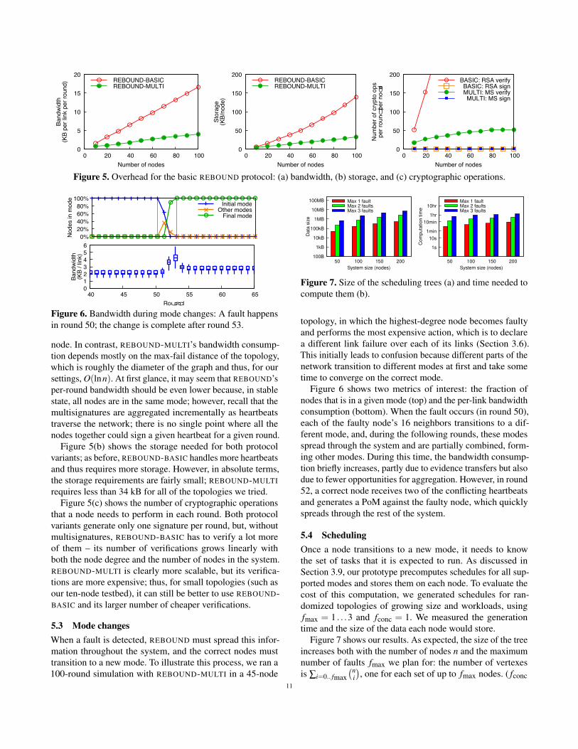
5.2 Bandwidth and computation

Even in the absence of faults, REBOUND imposes a cost on

the system, by generating and processing heartbeats, and by

storing information about modes. To quantify this cost, we ini-

tially ran both REBOUND-BASIC and REBOUND-MULTI with-

out a higher-level protocol. We ran simulations for 50 rounds

using our synthetic networks and both protocol variants for

each topology; we measured, for each node, the storage con-

sumption and the frequency of the cryptographic operations,

as well as the bandwidth per link. All measurements were

taken in the final round, that is, in steady state.

Figure 5(a) shows our results for bandwidth. REBOUND-

BASIC requires a lot of network traffic: its bandwidth con-

sumption grows linearly with the number of nodes, since each

node must forward and verify a heartbeat from every other

10

0

5

10

15

20

0 20 40 60 80 100

Bandwidth

(KB

per link per round)

Number of nodes

REBOUND-BASIC

REBOUND-MULTI

0

50

100

150

200

0 20 40 60 80 100

Storage

(KB/node)

Number of nodes

REBOUND-BASIC

REBOUND-MULTI

0

50

100

150

200

0 20 40 60 80 100

Number of crypto

ops

per round

per node

Number of nodes

BASIC: RSA verifyBASIC: RSA signMULTI: MS verifyMULTI: MS sign

Figure 5. Overhead for the basic REBOUND protocol: (a) bandwidth, (b) storage, and (c) cryptographic operations.

0%

20%

40%

60%

80%

100%

Nodes in mode

Initial mode

Other modes

Final mode

0

1

2

3

4

5

6

40 45 50 55 60 65

Bandwidth

(KB

/ link)

Round

Figure 6. Bandwidth during mode changes: A fault happens

in round 50; the change is complete after round 53.

node. In contrast, REBOUND-MULTI’s bandwidth consump-

tion depends mostly on the max-fail distance of the topology,

which is roughly the diameter of the graph and thus, for our

settings, O(lnn). At first glance, it may seem that REBOUND’s

per-round bandwidth should be even lower because, in stable

state, all nodes are in the same mode; however, recall that the

multisignatures are aggregated incrementally as heartbeats

traverse the network; there is no single point where all the

nodes together could sign a given heartbeat for a given round.

Figure 5(b) shows the storage needed for both protocol

variants; as before, REBOUND-BASIC handles more heartbeats

and thus requires more storage. However, in absolute terms,

the storage requirements are fairly small; REBOUND-MULTI

requires less than 34 kB for all of the topologies we tried.

Figure 5(c) shows the number of cryptographic operations

that a node needs to perform in each round. Both protocol

variants generate only one signature per round, but, without

multisignatures, REBOUND-BASIC has to verify a lot more

of them – its number of verifications grows linearly with

both the node degree and the number of nodes in the system.

REBOUND-MULTI is clearly more scalable, but its verifica-

tions are more expensive; thus, for small topologies (such as

our ten-node testbed), it can still be better to use REBOUND-

BASIC and its larger number of cheaper verifications.

5.3 Mode changes

When a fault is detected, REBOUND must spread this infor-

mation throughout the system, and the correct nodes must

transition to a new mode. To illustrate this process, we ran a

100-round simulation with REBOUND-MULTI in a 45-node

100B

1kB

10kB

100kB

1MB

10MB

100MB

50 100 150 200

Data

siz

e

System size (nodes)

Max 1 faultMax 2 faultsMax 3 faults

1s

10s

1min

10min

1hr

10hr

50 100 150 200

Com

puta

tion

tim

e

System size (nodes)

Max 1 faultMax 2 faultsMax 3 faults

Figure 7. Size of the scheduling trees (a) and time needed to

compute them (b).

topology, in which the highest-degree node becomes faulty

and performs the most expensive action, which is to declare

a different link failure over each of its links (Section 3.6).

This initially leads to confusion because different parts of the

network transition to different modes at first and take some

time to converge on the correct mode.

Figure 6 shows two metrics of interest: the fraction of

nodes that is in a given mode (top) and the per-link bandwidth

consumption (bottom). When the fault occurs (in round 50),

each of the faulty node’s 16 neighbors transitions to a dif-

ferent mode, and, during the following rounds, these modes

spread through the system and are partially combined, form-

ing other modes. During this time, the bandwidth consump-

tion briefly increases, partly due to evidence transfers but also

due to fewer opportunities for aggregation. However, in round

52, a correct node receives two of the conflicting heartbeats

and generates a PoM against the faulty node, which quickly

spreads through the rest of the system.

5.4 Scheduling

Once a node transitions to a new mode, it needs to know

the set of tasks that it is expected to run. As discussed in

Section 3.9, our prototype precomputes schedules for all sup-

ported modes and stores them on each node. To evaluate the

cost of this computation, we generated schedules for ran-

domized topologies of growing size and workloads, using

fmax = 1 . . .3 and fconc = 1. We measured the generation

time and the size of the data each node would store.

Figure 7 shows our results. As expected, the size of the tree

increases both with the number of nodes n and the maximum

number of faults fmax we plan for: the number of vertexes

is ∑i=0.. fmax

(

ni

)

, one for each set of up to fmax nodes. ( fconc

11

0

1

2

3

4

5

Unprot 1 2 3

.007

Avg bandwidth

(KB/round,node)

Parameter fconc

AuditingREBOUNDPayload

(a) Bandwidth

0

2

4

6

8

10

12

14

16

18

Unprot 1 2 3Avg computation (ops/round,node)

Parameter fconc

Auditing RSA SignAuditing RSA VrfyREBOUND MS SignREBOUND MS Vrfy

(b) Computation

0

10

20

30

40

50

60

70

80

90

Unprot 1 2 3

Avg storage (KB/node)

Parameter fconc

AuditingREBOUNDPayload

(c) Storage

Figure 8. Average per-node runtime costs in the case study.

does not affect the number of vertexes, but it does increase the

number of edges.) In absolute terms, the schedules are only a

few MB in size, which can easily fit into the available flash

memory on many embedded devices. Schedules take between

a few minutes and an hour to generate, but this process is

entirely offline and is only done once.

5.5 Auditing

Next, we examined the overall cost of a BTR deployment,

including both REBOUND-MULTI and auditing. We used an

example system containing 26 nodes with 4 application flows

and ran it for 100 rounds, using the EDF scheduler in our

simulator. We looked at two variants: a normal, unprotected

system, and one with REBOUND-MULTI and auditing enabled,

and configured to protect against fconc = 1 . . .3 concurrent

faults. We measured the number of cryptographic operations,

the amount of RAM needed for the protocol (not including

the flash memory for the scheduling tree, which was already

covered above), and the average per-node network bandwidth.

Figure 8 shows our results. The unprotected system gener-

ates fairly little traffic and has no cryptographic operations.

Enabling REBOUND adds a fixed overhead, independent of

fconc; in addition, each replica needs to store a copy of the

primary’s state, and the primary needs to stream updates to

each replica. There is a small O( f 2conc) term because, when

the primary receives a message m, it, and each of its replicas,

must relay the m’s authenticator to the sender’s replicas, but

this term is not dominant for small values of fconc.

We note that each replica must also replay the primary’s

computation to verify that the primary behaved as expected.

This overhead is trivially linear in fconc because each task

is effectively executed fconc +1 times: once by the original

node and once by each of the replicas.

5.6 Comparison to BFT

Next, we discuss how REBOUND compares to classical Byzan-

tine fault tolerance (BFT). On comparable hardware, BFT

protocols would not be able to run as many applications

as REBOUND because they require more replicas – 3 f + 1

in the case of asynchronous protocols, such as the popular

PBFT [25], and 2 f +1 in the case of synchronous protocols,

such as [2], which also require fewer rounds. To illustrate this,

0

0.5

1

1.5

2

2.5

3

3.5

f=1 f=2 f=3

Supported

workload

(normalized

to

PBFT)

Parameter f

PBFTREBOUND(3f+1)/(f+1)

Figure 9. Comparison to PBFT.

0

20

40

60

80

100

0 1 2 3

Ve

locity (

mp

h)

Time (s)

(a)

0

20

40

60

80

100

0 1 2 3

Time (s)(b)

0

20

40

60

80

100

0 1 2 3

Time (s)(c)

64.6

64.8

65

65.2

65.4

0

50

10

0

15

0

Time (ms)(d)

Figure 10. Simulated Volvo XC90 velocity, with cruise con-

trol set to 65mph, (a) during normal operation, (b) during an

attack, and (c) with REBOUND. (d) shows a detail of (c).

we derived scheduling constraints for PBFT analogous to Sec-

tion 3.9 (see [51, §F]); then we randomly generated 75 work-

loads and scheduled them on systems with N = 25, . . . ,75

nodes, using either PBFT or REBOUND as a defense. In both

cases, we generated more tasks than the systems could handle,

and we allowed the schedulers to drop any excess tasks, so

the systems were packed with as many tasks as possible. We

then measured the median total utilization of the tasks without

replicas – that is, how many nodes’ worth of useful work the

system can do.

Figure 9 shows our results. The numbers are normalized to

the workload that PBFT can support. As expected, REBOUND

can, on a given system, run workloads that are at least twice

as big as PBFT’s. The ratio closely tracks3 f+1f+1

(shown as

circles); for large f , it would eventually approach 3. In a

comparison to a synchronous BFT protocol, the ratio would

approach 2 instead.

5.7 Case study: Volvo XC90

Next, we examine how much damage the adversary can do in

a concrete CPS with and without REBOUND. We use a car –

specifically, the Volvo XC90 – as a case study; given several

widely publicized hacks of cars [30, 48, 49, 80, 99, 119],

this seemed like an interesting use case. The XC90 has 38

compute nodes and 13 buses – 1 HCAN, 1 LCAN, 1 MOST,

and 10 LIN – for connectivity. The only modification we

made was to move the sensors and actuators, which were

originally connected directly to specific ECUs, directly onto

the CAN buses, so they could also communicate with other

ECUs. This change would not be difficult to make in a real

car, and it is critical to enabling recovery (otherwise there is a

single point of failure).

12

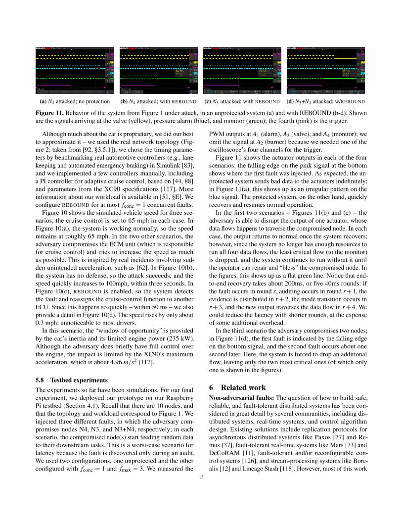
(a) N4 attacked; no protection (b) N4 attacked; with REBOUND (c) N3 attacked; with REBOUND (d) N3+N4 attacked; w/REBOUND

Figure 11. Behavior of the system from Figure 1 under attack, in an unprotected system (a) and with REBOUND (b-d). Shown

are the signals arriving at the valve (yellow), pressure alarm (blue), and monitor (green); the fourth (pink) is the trigger.

Although much about the car is proprietary, we did our best

to approximate it – we used the real network topology (Fig-

ure 2; taken from [92, §3.5.1]), we chose the timing parame-

ters by benchmarking real automotive controllers (e.g., lane

keeping and automated emergency braking) in Simulink [83],

and we implemented a few controllers manually, including

a PI controller for adaptive cruise control, based on [44, 88]

and parameters from the XC90 specifications [117]. More

information about our workload is available in [51, §E]. We

configure REBOUND for at most fconc = 1 concurrent faults.

Figure 10 shows the simulated vehicle speed for three sce-

narios; the cruise control is set to 65 mph in each case. In

Figure 10(a), the system is working normally, so the speed

remains at roughly 65 mph. In the two other scenarios, the

adversary compromises the ECM unit (which is responsible

for cruise control) and tries to increase the speed as much

as possible. This is inspired by real incidents involving sud-

den unintended acceleration, such as [62]. In Figure 10(b),

the system has no defense, so the attack succeeds, and the

speed quickly increases to 100mph, within three seconds. In

Figure 10(c), REBOUND is enabled, so the system detects

the fault and reassigns the cruise-control function to another

ECU. Since this happens so quickly – within 50 ms – we also

provide a detail in Figure 10(d). The speed rises by only about

0.3 mph; unnoticeable to most drivers.

In this scenario, the “window of opportunity” is provided

by the car’s inertia and its limited engine power (235 kW).

Although the adversary does briefly have full control over

the engine, the impact is limited by the XC90’s maximum

acceleration, which is about 4.96 m/s2 [117].

5.8 Testbed experiments

The experiments so far have been simulations. For our final

experiment, we deployed our prototype on our Raspberry

Pi testbed (Section 4.1). Recall that there are 10 nodes, and

that the topology and workload correspond to Figure 1. We

injected three different faults, in which the adversary com-

promises nodes N4, N3, and N3+N4, respectively; in each

scenario, the compromised node(s) start feeding random data

to their downstream tasks. This is a worst-case scenario for

latency because the fault is discovered only during an audit.

We used two configurations, one unprotected and the other

configured with fconc = 1 and fmax = 3. We measured the

PWM outputs at A1 (alarm), A3 (valve), and A4 (monitor); we

omit the signal at A2 (burner) because we needed one of the

oscilloscope’s four channels for the trigger.

Figure 11 shows the actuator outputs in each of the four

scenarios; the falling edge on the pink signal at the bottom

shows where the first fault was injected. As expected, the un-

protected system sends bad data to the actuators indefinitely;

in Figure 11(a), this shows up as an irregular pattern on the

blue signal. The protected system, on the other hand, quickly

recovers and resumes normal operation.

In the first two scenarios – Figures 11(b) and (c) – the

adversary is able to disrupt the output of one actuator, whose

data flows happens to traverse the compromised node. In each

case, the output returns to normal once the system recovers;

however, since the system no longer has enough resources to

run all four data flows, the least critical flow (to the monitor)

is dropped, and the system continues to run without it until

the operator can repair and “bless” the compromised node. In

the figures, this shows up as a flat green line. Notice that end-

to-end recovery takes about 200ms, or five 40ms rounds: if

the fault occurs in round r, auditing occurs in round r+1, the

evidence is distributed in r+2, the mode transition occurs in

r+3, and the new output traverses the data flow in r+4. We

could reduce the latency with shorter rounds, at the expense

of some additional overhead.

In the third scenario the adversary compromises two nodes;

in Figure 11(d), the first fault is indicated by the falling edge

on the bottom signal, and the second fault occurs about one

second later. Here, the system is forced to drop an additional

flow, leaving only the two most critical ones (of which only

one is shown in the figures).

6 Related work

Non-adversarial faults: The question of how to build safe,

reliable, and fault-tolerant distributed systems has been con-

sidered in great detail by several communities, including dis-

tributed systems, real-time systems, and control algorithm

design. Existing solutions include replication protocols for

asynchronous distributed systems like Paxos [77] and Re-

mus [37], fault-tolerant real-time systems like Mars [73] and

DeCoRAM [11], fault-tolerant and/or reconfigurable con-

trol systems [126], and stream-processing systems like Bore-

alis [12] and Lineage Stash [118]. However, most of this work

13

has considered various types of “benign” faults, such as hard-

ware defects, software bugs, or electromagnetic interference,

whereas we focus on attacks by a malicious adversary.

Byzantine fault tolerance: There is a rich literature on pro-

tocols for tolerating Byzantine faults [1, 5, 25, 33, 36, 56,

63, 74, 79, 105, 114, 121, 123], and some of these protocols

have been applied to time-critical distributed systems (e.g.,

in [65, 72, 87]). Many common BFT protocols are asynchro-

nous and thus cannot provide timing guarantees systems, espe-

cially under attack [104], although more recent protocols have

improved in this respect [8, 34]. There are, however, protocols

for partially synchronous systems, such as [86, 124], as well

as fully synchronous protocols, such as [2]. BFT++ [84] is ex-

plicitly designed for BFT in CPS, but is somewhat constrained

because it is designed to also work with legacy systems. The

fault-tolerance approach is complementary to BTR: it can

fully mask the symptoms of certain attacks, but it requires

more replicas and stronger assumptions.

Classical recovery: There is substantial prior work on re-

covering systems from intrusions when there are no timing

constraints. For instance, Warp [26] can retroactively patch

security vulnerabilities in database-backed web applications

by rolling back the database and replaying inputs using the

patched code, and Retro [71] can repair desktop or server ma-

chines by selectively undoing the adversary’s changes while

preserving legitimate actions. Unlike REBOUND, these sys-

tems cannot guarantee time bounds on recovery, but they do

reinforce our earlier point that repairing incorrect outputs is

often possible, even outside of CPS.

Bounded-time recovery: The idea of systems recovering in

bounded time goes back to work on real-time databases [103].

SAUCR [6] observes that most consecutive data center faults

are spaced more than 50 ms apart; it switches from a high-

performance to high-safety mode when a fault occurs and

switches back once recovery occurs. Cascade [50] looks at

bounded-time recovery in a broader set of applications that

includes CPS, but, like SAUCR, it is limited to crash faults.

We had speculated earlier [31] that BTR could be generalized

to Byzantine faults but, to our knowledge, REBOUND is the

first concrete solution.

Self-stabilization: One way to make a distributed system

fault-tolerant is to ensure that it converges to a correct state

even if it is started in an incorrect state. This approach was

first proposed by Dijkstra [39] and has led to a rich body of

work on self-stabilizing systems [4, 20, 22, 41, 42, 54, 55, 66,

69, 76]. Much of the early work assumed that faults are be-

nign and cannot handle malicious nodes that might constantly

steer the system away from its goal. Recent work [14, 38,

40, 43, 64, 82] has extended the approach to the Byzantine

setting, but this line of work tends to use a very different

system model: for instance, it often relies on a global reset

mechanism for recovery, it typically does not consider sched-

uling, deadlines, or task criticality, and it does not provide a

time bound for recovery.

Failure detectors: There is an impressive amount of work

on fault detection in the context of failure detectors, starting

from a paper by Chandra and Toueg [28], but this litera-

ture conventionally assumes benign crash faults, and usually

studies theoretical bounds on the information about failures

that is necessary to solve various distributed computing prob-

lems [27]. Kihlstrom et al. [70] was the first to focus explicitly

on Byzantine faults, but the definitions in [70] are specific

to consensus and broadcast protocols. Haeberlen et al. [60]

generalized this concept but focused exclusively on the asyn-

chronous setting, without time bounds or support for recovery.

Attack-resistant control: There is an emerging security-

oriented research trend within the control and CPS communi-

ties (e.g., see [45] and the references therein). However, exist-

ing solutions either assume a centralized setting (e.g., [120])

or focus more on attacks on the sensors and actuators, and

not on the controllers (e.g., [7, 23, 45, 89, 109]); the latter

approach is complementary to ours.

Accountability: Accountability [3, 10, 58–61, 127] provides

a way to detect many forms of Byzantine behavior, and it can

also generate evidence of detected attacks. However, all of

the existing work on accountability assumes an asynchronous

system, that is, it cannot detect timing faults, give a bound on

the time to detection, or perform recovery.

Multi-mode systems: Many real-time embedded systems

can operate in multiple modes that involve different sets of

tasks, and transitioning between modes requires elaborate

mode-change protocols (MCPs) to prevent deadline misses

and other disruptions [47, 96, 98, 102, 107, 112]. Our recov-

ery approach builds on MCPs; however, to our knowledge, all

the existing work on MCPs assumes benign faults and cannot

work reliably when the system is compromised.

7 Conclusion

We believe that REBOUND can be an interesting new tool

in the community’s toolbox for handling Byzantine faults.

Although we have demonstrated REBOUND in the context of

cyber-physical systems, our approach (and REBOUND itself)

is not limited to that domain – it should be applicable to any

system that can tolerate bad outputs for a very brief period,

such as stream processing or video streaming. As we have

shown, there are valuable benefits to be had – including a

lower overhead, timing guarantees, a wider range for fmax,

and the ability to support gradual degradation.

Acknowledgments

We thank our shepherd, Manos Kapritsos, and the anonymous

reviewers for their thoughtful comments and suggestions.

This work was supported in part by NSF grants CNS-1563873,

CNS-1703936, CNS-1750158, and CNS-1955670, and by

ONR N00014-20-1-2744.

14

References[1] M. Abd-El-Malek, G. R. Ganger, G. R. Goodson, M. K. Reiter, and

J. J. Wylie. Fault-scalable Byzantine fault-tolerant services. In Proc.

SOSP, 2005.

[2] I. Abraham, D. Malkhi, K. Nayak, L. Ren, and M. Yin. Sync HotStuff:

Simple and practical synchronous state machine replication. In Proc.

Oakland, 2020.

[3] P. Aditya, M. Zhao, Y. Lin, A. Haeberlen, P. Druschel, B. Maggs, and

B. Wishon. Reliable client accounting for hybrid content-distribution

networks. In Proc. NSDI, 2012.

[4] Y. Afek and G. M. Brown. Self-stabilization over unreliable commu-

nication media. Distributed Computing, 7(1):27–3–4, 1993.

[5] A. S. Aiyer, L. Alvisi, A. Clement, M. Dahlin, J.-P. Martin, and

C. Porth. BAR fault tolerance for cooperative services. In Proc. SOSP,

2005.

[6] R. Alagappan, A. Ganesan, J. Liu, A. Arpaci-Dusseau, and R. Arpaci-

Dusseau. Fault-tolerance, fast and slow: Exploiting failure asynchrony

in distributed systems. In OSDI, 2018.

[7] S. Amin, A. A. Cárdenas, and S. S. Sastry. Safe and secure networked

control systems under denial-of-service attacks. In Proc. HSCC, 2009.

[8] Y. Amir, B. Coan, J. Kirsch, and J. Lane. Prime: Byzantine repli-

cation under attack. IEEE Transactions on Dependable and Secure

Computing (TDSC), 8(4):564–577, 2011.

[9] Z. Anderson and M. Giovanardi. Self-driving vehicle with integrated

active suspension, Oct. 2 2014. US Patent App. 14/242,691.

[10] M. Backes, P. Druschel, A. Haeberlen, and D. Unruh. CSAR: a practi-

cal and provable technique to make randomized systems accountable.

In Proc. NDSS, 2009.

[11] J. Balasubramanian, A. Gokhale, A. Dubey, F. Wolf, D. C. Schmidt,

C. Lu, and C. Gill. Middleware for resource-aware deployment and

configuration of fault-tolerant real-time systems. In Proc. RTAS, 2010.

[12] M. Balazinska, H. Balakrishnan, S. R. Madden, and M. Stonebraker.

Fault-tolerance in the borealis distributed stream processing system.

ACM Trans. Database Syst., 33(1):3:1–3:44, Mar. 2008.

[13] Ben Lynn. PBC Library. Version 0.5.14.

[14] M. Ben-Or, D. Dolev, and E. N. Hoch. Fast self-stabilizing Byzantine

tolerant digital clock synchronization. In Proc. PODC, 2008.

[15] T. Besselmann and M. Morari. Hybrid Parameter-Varying MPC

for Autonomous Vehicle Steering. European Journal of Control,

14(5):418 – 431, 2008.

[16] A. Bhat, S. Samii, and R. Rajkumar. Practical task allocation for soft-

ware fault-tolerance and its implementation in embedded automotive

systems. In Proc. RTAS, 2017.

[17] A. Boldyreva. Threshold signatures, multisignatures and blind signa-

tures based on the Gap-Diffie-Hellman group signature scheme. In

Proc. PKC, 2003.

[18] F. Borrelli, A. Bemporad, M. Fodor, and D. Hrovat. An MPC/Hybrid

System Approach to Traction Control. IEEE Transactions on Control

Systems Technology, 14(3):541 – 552, May 2006.

[19] G. Bracha. An asynchronous ⌊(n−1)/3⌋-resilient consensus protocol.

In Proc. PODC, 1984.

[20] G. M. Brown, M. G. Gouda, and C.-L. Wu. Token systems that

self-stabilize. IEEE Trans. Comput., 38(6):845–852, June 1989.

[21] A. Burns and R. I. Davis. Mixed criticality systems – a review. http:

//www-users.cs.york.ac.uk/burns/review.pdf, Mar. 2019.

[22] J. E. Burns and J. K. Pachl. Uniform self-stabilizing rings. ACM

Transations on Programming Languages and Systems, 11(2):330–344,

Apr. 1989.

[23] A. A. Cárdenas, S. Amin, and S. Sastry. Research challenges for the

security of control systems. In Proc. HotSec, 2008.

[24] J. Carrau, A. Liniger, X. Zhang, and J. Lygeros. Efficient Implemen-

tation of Randomized MPC for Miniature Race Cars. In European

Control Conference (ECC), 2016.

[25] M. Castro and B. Liskov. Practical Byzantine fault tolerance and proac-

tive recovery. ACM Transactions on Computer Systems, 20(4):398–

461, 2002.

[26] R. Chandra, T. Kim, M. Shah, N. Narula, and N. Zeldovich. Intrusion

recovery for database-backed web applications. In Proc. SOSP, 2011.

[27] T. D. Chandra, V. Hadzilacos, and S. Toueg. The weakest failure

detector for solving consensus. J. ACM, 43(4):685–722, July 1996.

[28] T. D. Chandra and S. Toueg. Unreliable failure detectors for reliable

distributed systems. J. ACM, 43(2):225–267, Mar. 1996.

[29] R. N. Charette. This car runs on code. IEEE Spectrum, 2009. http:

//spectrum.ieee.org/transportation/systems/this-car-runs-on-code.

[30] S. Checkoway, D. McCoy, B. Kantor, D. Anderson, H. Shacham,

S. Savage, K. Koscher, A. Czeskis, F. Roesner, and T. Kohno. Com-

prehensive experimental analyses of automotive attack surfaces. In

Proc. USENIX Security, 2011.

[31] A. Chen, H. Xiao, L. T. X. Phan, and A. Haeberlen. Fault tolerance

and the five-second rule. In Proc. HotOS, May 2015.

[32] J. Chen, R. Tan, G. Xing, and X. Wang. PTEC: A system for predictive

thermal and energy control in data centers. In Proc. RTSS, 2014.

[33] B.-G. Chun, P. Maniatis, S. Shenker, and J. Kubiatowicz. Attested

append-only memory: Making adversaries stick to their word. In Proc.

SOSP, 2007.

[34] A. Clement, E. L. Wong, L. Alvisi, M. Dahlin, and M. Marchetti.

Making Byzantine fault tolerant systems tolerate Byzantine faults. In

Proc. NSDI, 2009.

[35] R. P. Collinson. Introduction to avionics systems. Springer, 2011.

[36] J. A. Cowling, D. S. Myers, B. Liskov, R. Rodrigues, and L. Shrira. HQ

replication: A hybrid quorum protocol for Byzantine fault tolerance.

In Proc. OSDI, 2006.

[37] B. Cully, G. Lefebvre, D. Meyer, M. Feeley, N. Hutchinson, and

A. Warfield. Remus: high availability via asynchronous virtual ma-

chine replication. In Proc. NSDI, 2008.

[38] A. Daliot and D. Dolev. Self-stabilization of Byzantine protocols. In

Proc. SSS, 2005.

[39] E. W. Dijkstra. Self-stabilizing systems in spite of distributed control.

Communications of the ACM, 17(11):643–644, Nov. 1974.

[40] D. Dolev and E. N. Hoch. Byzantine self-stabilizing pulse in a

bounded-delay model. In Proc. SSS, 2007.

[41] S. Dolev. Self-Stabiliaztion. MIT Press, 2000.

[42] S. Dolev, A. Israeli, and S. Moran. Self-stabilization of dynamic

systems assuming only read/write atomicity. In Proc. PODC, 1990.

[43] S. Dolev and J. L. Welch. Self-stabilizing clock synchronization in

the presence of Byzantine faults. J. ACM, 51(5):780–799, Sept. 2004.

[44] U. Drolia, Z. Wang, Y. Pant, and R. Mangharam. Autoplug: An auto-

motive test-bed for electronic controller unit testing and verification.

In Proc. ITSC, 2011.

[45] H. Fawzi, P. Tabuada, and S. Diggavi. Secure estimation and

control for cyber-physical systems under adversarial attacks. In

arXiv:1025.5073v1, 2012.

[46] M. J. Fischer, N. A. Lynch, and M. S. Paterson. Impossibility of

distributed consensus with one faulty process. J. ACM, 32(2):374–

382, Apr. 1985.

[47] G. Fohler. Changing operational modes in the context of pre-runtime

scheduling. IEICE Transactions on Information and Systems, E76-

D(11):1333–1340, 1993.

[48] I. Foster, A. Prudhomme, K. Koscher, and S. Savage. Fast and vulner-

able: A story of telematic failures. In Proc. WOOT, 2015.

[49] L. Franceschi-Bichhierai. Hacker finds he can remotely kill

car engines after breaking into GPS tracking apps, 2019.

https://www.vice.com/en_us/article/zmpx4x/hacker-monitor-cars-kill-

engine-gps-tracking-apps.

[50] N. Gandhi, E. Roth, R. Gifford, L. T. X. Phan, and A. Haeberlen.

Bounded-time recovery for distributed real-time systems. In Proc.

RTAS, 2020.

15

[51] N. Gandhi, E. Roth, B. Sandler, A. Haeberlen, and L. T. X. Phan. RE-

BOUND: Defending distributed systems against attacks with bounded-

time recovery (extended version). Technical Report MS-CIS-21-01,

Department of Computer and Information Science, University of Penn-

sylvania, 2021.

[52] T. Geyer, G. Papafotiou, R. Frasca, and M. Morari. Constrained Opti-

mal Control of the Step-Down DC-DC Converter. IEEE Transactions

on Power Electronics, 23(5):2454–2464, Sept. 2008.

[53] T. Geyer, G. Papafotiou, and M. Morari. Model Predictive Direct

Torque Control - Part I: Concept, Algorithm and Analysis. IEEE

Trans. on Industrial Electronics, 56(6):1894–1905, June 2009.

[54] M. Gouda and N. Multari. Stabilizing communication protocols. IEEE

Transactions on Computers, 40(4):448–458, Apr. 1991.

[55] M. G. Gouda, R. R. Howell, and L. E. Rosier. The instability of

self-stabilization. Acta Informatica, 27(8):697–724, 1990.

[56] R. Guerraoui, N. Kneževic, V. Quéma, and M. Vukolic. The next 700

BFT protocols. In Proc. EuroSys, 2010.

[57] Gurobi Optimization, Inc. http://www.gurobi.com.

[58] A. Haeberlen, P. Aditya, R. Rodrigues, and P. Druschel. Accountable

virtual machines. In Proc. OSDI, 2010.

[59] A. Haeberlen, I. Avramopoulos, J. Rexford, and P. Druschel. NetRe-

view: Detecting when interdomain routing goes wrong. In Proc. NSDI,

2009.

[60] A. Haeberlen and P. Kuznetsov. The Fault Detection Problem. In

Proc. OPODIS, Dec. 2009.

[61] A. Haeberlen, P. Kuznetsov, and P. Druschel. PeerReview: Practical

accountability for distributed systems. In Proc. SOSP, 2007.

[62] L. Ham and R. Grace. Cruise control terror for freeway driver. The

Sydney Morning Herald, Dec. 2009. https://www.smh.com.au/national/

cruise-control-terror-for-freeway-driver-20091215-ktxn.html.

[63] C. Ho, R. van Renesse, M. Bickford, and D. Dolev. Nysiad: Practical

protocol transformation to tolerate Byzantine failures. In Proc. NSDI,

2008.

[64] E. N. Hoch, D. Dolev, and A. Daliot. Self-stabilizing Byzantine digital

clock synchronization. In Proc. SSS, 2006.

[65] K. Hoyme and K. Driscoll. SAFEbus. In Proc. DASC, 1992.

[66] A. Israeli and M. Jalfon. Token management schemes and random

walks yield self-stabilizing mutual exclusion. In Proc. PODC, 1990.

[67] K. Itakura and K. Nakamura. A public key cryptosystem suitable for

digital multisignatures. NEC Research & Development, 71:1–8, 1983.

[68] K. Jang, J. Sherry, H. Ballani, and T. Moncaster. Silo: Predictable

message latency in the cloud. In Proc. SIGCOMM, 2015.

[69] S. Katz and K. J. Perry. Self-stabilizing extensions for message-

passing systems. Distributed Computing, 7(1):17–26, Nov. 1993.

[70] K. P. Kihlstrom, L. E. Moser, and P. M. Melliar-Smith. Byzantine fault

detectors for solving consensus. The Computer Journal, 46(1):16–35,

2003.

[71] T. Kim, X. Wang, N. Zeldovich, and M. F. Kaashoek. Intrusion

recovery using selective re-execution. In Proc. OSDI, 2010.

[72] H. Kopetz and G. Bauer. The time-triggered architecture. Proceedings

of the IEEE, 91(1):112–126, 2003.

[73] H. Kopetz, A. Damm, C. Koza, M. Mulazzani, W. Schwabl, C. Senft,

and R. Zainlinger. Distributed fault-tolerant real-time systems: The

Mars approach. IEEE Micro, 9(1):25–40, 1989.

[74] R. Kotla, L. Alvisi, M. Dahlin, A. Clement, and E. L. Wong. Zyzzyva:

Speculative Byzantine fault tolerance. ACM Transactions on Com-

puter Systems (TOCS), 27(4), 2009.

[75] E. Kovacs. Cyberattack on german steel plant caused significant dam-

age. Security Week, 2014. https://www.securityweek.com/cyberattack-

german-steel-plant-causes- significant-damage-report.

[76] H. Kruijer. Self-stabilization (in spite of distributed control) in tree-

structured systems. Information Processing Letters, 8(2):91–95, 1979.

[77] L. Lamport. The part-time parliament. ACM Transactions on Com-

puter Systems (TOCS), 16(2):133–169, May 1998.

[78] L. Lamport, R. Shostak, and M. Pease. The Byzantine generals prob-

lem. ACM Transactions on Programming Languages and Systems

(TOPLAS), 4(3):382–401, 1982.

[79] J. Li and D. Mazières. Beyond one-third faulty replicas in Byzantine

fault tolerant systems. In Proc. NSDI, 2007.

[80] M. Liebowitz. The sound of hacking: Researchers use Trojan CD to

hack car. NBC News, 2011. http://www.nbcnews.com/id/42074718/ns/

technology_and_science-security/t/sound-hacking-researchers-use-

trojan-cd-hack-car/#.XYPOBSUpDUY.

[81] F. Maggi. Rogue robots: Testing the limits of an industrial robot’s

security. TrendLabs, https://www.dropbox.com/s/7ob04tbhpdjj6ks/tr.

pdf, 2017.

[82] M. R. Malekpour. A Byzantine-fault tolerant self-stabilizing protocol

for distributed clock synchronization systems. In Proc. SSS, 2006.

[83] MATLAB. Version 9.7.0 (R2019b). The MathWorks Inc., Natick,

Massachusetts, 2019.

[84] J. S. Mertoguno, R. Craven, M. Mickelson, and D. Koller. A physics-

based strategy for cyber resilience of CPS. In Defense + Commercial

Sensing, 2019.

[85] S. Micali, K. Ohta, and L. Reyzin. Accountable-subgroup multisigna-

tures. In Proc. ACM CCS, 2001.

[86] Z. Milosevic, M. Biely, and A. Schiper. Bounded delay in Byzantine-

tolerant state machine replication. In Proc. SRDS, 2013.

[87] P. Miner. Analysis of the SPIDER fault-tolerance protocols. In Proc.

NASA Langley Formal Methods Workshop (LFM), 2000.

[88] mLAB. Autoplug. https://github.com/mlab-upenn/AutoPlug/blob/

master/Firmware/CruiseControl/Sources/main.c.

[89] Y. Mo and B. Sinopoli. Secure control against replay attacks. In

Proceedings of the Allerton Conference on Communication, Control,

and Computing (ALLERTON), 2009.

[90] M. Morari. Fast model predictive control (MPC). Presentation,

available from http://divf.eng.cam.ac.uk/cfes/pub/Main/Presentations/

Morari.pdf.

[91] NIST. Guide to supervisory control and data ac-

quisition (SCADA) and industrial control systems se-

curity, 2006. https://www.dhs.gov/sites/default/files/

publications/csd-nist-guidetosupervisoryanddataccquisition-

scadaandindustrialcontrolsystemssecurity-2007.pdf.

[92] T. Nolte. Share-driven scheduling of embedded networks, 2006.

[93] F. Oldewurtel, A. Ulbig, A. Parisio, G. Andersson, and M. Morari.

Reducing Peak Electricity Demand in Building Climate Control using

Real-Time Pricing and Model Predictive Control. In Proc. Conference

on Decision and Control (CDC), 2010.

[94] M. Pajic, J. Weimer, N. Bezzo, O. Sokolsky, G. J. Pappas, and I. Lee.

Design and implementation of attack-resilient cyberphysical systems:

With a focus on attack-resilient state estimators. IEEE Control Systems,

37(2):66–81, April 2017.

[95] G. Papafotiou, J. Kley, K. Papadopoulos, P. Bohren, and M. Morari.

Model Predictive Direct Torque Control - Part II: Implementation

and Experimental Evaluation. IEEE Trans. on Industrial Electronics,

56(6):1906–1915, June 2009.

[96] P. Pedro and A. Burns. Schedulability analysis for mode changes in

flexible real-time systems. In Proc. ECRTS, 1998.

[97] P. Ramanathan and M. Hamdaoui. A dynamic priority assignment

technique for streams with (m, k)-firm deadlines. IEEE Transactions

on Computers, 44(12):1443–1451, 1995.

[98] J. Real and A. Crespo. Mode change protocols for real-time systems:

A survey and a new proposal. Real-Time Systems, 26:161–197, 2004.

[99] J. Reindl. Car hacking remains a very real threat as autos be-

come ever more loaded with tech. USA Today, 2018. https:

//www.usatoday.com/story/money/2018/01/14/car-hacking-remains-

very-real-threat-autos- become-ever-more-loaded-tech/1032951001/.

[100] S. Richter, S. Mariethoz, and M. Morari. High-speed online MPC

based on a fast gradient method applied to power converter control.

16

In Proc. American Control Conference, 2010.

[101] E. Roth and A. Haeberlen. Do not overpay for fault tolerance! In Proc.

RTAS, 2021.

[102] L. Sha, R. Rajkumar, J. Lehoczky, and K. Ramamritham. Mode

change protocols for priority-driven preemptive scheduling. Real-

Time Systems, 1(3):243–264, 1989.

[103] L. C. Shu, J. A. Stankovic, and S. H. Son. Achieving bounded and

predictable recovery using real-time logging. In Proc. RTAS, 2002.

[104] A. Singh, T. Das, P. Maniatis, P. Druschel, and T. Roscoe. BFT

protocols under fire. In Proc. NSDI, 2008.

[105] A. Singh, P. Fonseca, P. Kuznetsov, R. Rodrigues, and P. Maniatis.

Zeno: Eventually consistent Byzantine-fault tolerance. In Proc. NSDI,

2009.

[106] D. Soudbakhsh, L. T. X. Phan, A. Annaswamy, O. Sokolsky, and

I. Lee. Co-design of control and platform with dropped signals. In

Proc. ICCPS, Apr. 2013.

[107] N. Stoimenov, S. Perathoner, and L. Thiele. Reliable mode changes

in real-time systems with fixed priority or EDF scheduling. In Proc.

DATE, 2009.

[108] G.-N. Sung, C.-Y. Juan, and C.-C. Wang. Bus guardian design for

automobile networking ECU nodes compliant with FlexRay standards.

In Proc. ISCE, 2008.

[109] A. Teixeira, D. Pérez, H. Sandberg, and K. H. Johansson. Attack

models and scenarios for networked control systems. In Proc. HiCoNS,

2012.

[110] C. Temple. Avoiding the babbling-idiot failure in a time-triggered

communication system. In Proc. FTCS, 1998.

[111] D. Tesar. Robot and robot actuator module therefor, Oct. 18 1994. US

Patent 5,355,743.

[112] K. Tindell, A. Burns, and A. Wellings. Mode changes in priority

preemptively scheduled systems. In Proc. RTSS, 1992.

[113] L. Valenta, S. Cohney, A. Liao, J. Fried, S. Bodduluri, and N. Heninger.

Factoring as a service. Cryptology ePrint Archive, Report 2015/1000,

2015. https://eprint.iacr.org/2015/1000.

[114] B. Vandiver, H. Balakrishnan, B. Liskov, and S. Madden. Tolerat-

ing Byzantine faults in transaction processing systems using commit

barrier scheduling. In Proc. SOSP, 2007.

[115] M. Vasak, M. Baotic, M. Morari, I. Petrovic, and N. Peric. Constrained

optimal control of an electronic throttle. International Journal of

Control, 79(5):465–478, June 2006.

[116] S. Vestal. Preemptive scheduling of multi-criticality systems with

varying degrees of execution time assurance. In Proc. RTSS, 2007.

[117] Volvo. Xc90 technical data, 2018. Available from https://www.media.

volvocars.com/global/en-gb/models/xc90/2018/specifications.

[118] S. Wang, J. Liagouris, R. Nishihara, P. Moritz, U. Misra, A. Tumanov,

and I. Stoica. Lineage stash: fault tolerance off the critical path. In

Proc. SOSP, 2019.

[119] G. Warth. New hack: When drivers aren’t in control. San Diego Tri-

bune, 2015. https://www.sandiegouniontribune.com/news/education/

sdut-ucsd-professor-cyber-hacking-2015aug28-story.html.

[120] T. Wongpiromsarn, U. Topcu, and R. Murray. Receding horizon

temporal logic planning for dynamical systems. In Proceedings of the

48th IEEE Conference on Decision and Control (CDC), 2009.

[121] T. Wood, R. Singh, A. Venkataramani, P. Shenoy, and E. Cecchet. ZZ

and the art of practical BFT execution. In Proc. EuroSys, 2011.

[122] M. Xu, L. T. X. Phan, H. Y. Choi, and I. Lee. Analysis and implemen-

tation of global preemptive fixed-priority scheduling with dynamic

cache allocation. In Proc. RTAS, 2016.

[123] J. Yin, J.-P. Martin, A. Venkataramani, L. Alvisi, and M. Dahlin.

Separating agreement from execution for Byzantine fault tolerant

services. In Proc. SOSP, 2003.

[124] M. Yin, D. Malkhi, M. K. Reiter, G. G. Gueta, and I. Abraham. Hot-

Stuff: BFT consensus with linearity and responsivenes. In Proc.

PODC, 2019.

[125] M. Yu, L. Wang, T. Chu, and F. Hao. Stabilization of networked

control systems with data packet dropout and transmission delays:

Continuous-time case. European Journal of Control, 11(1):40–49,

2005.

[126] Y. Zhang and J. Jiang. Bibliographical review on reconfigurable fault-

tolerant control systems. Annual reviews in control, 32(2):229–252,

2008.

[127] W. Zhou, Q. Fei, A. Narayan, A. Haeberlen, B. T. Loo, and M. Sherr.

Secure network provenance. In Proc. SOSP, 2011.

17