Receding-horizon Stochastic Model Predictive Controlwith Hard Input Constraints and Joint State Chance

Constraints

Joel A. Paulsona,b, Edward A. Buehlerb, Richard D. Braatza, Ali Mesbahb

aDepartment of Chemical Engineering, Massachusetts Institute of Technology, Cambridge,MA 02139, USA

bDepartment of Chemical and Biomolecular Engineering, University of California-Berkeley,Berkeley, CA 94720, USA

Abstract

This article considers the stochastic optimal control of discrete-time lin-

ear systems subject to (possibly) unbounded stochastic disturbances, hard con-

straints on the manipulated variables, and joint chance constraints on the states.

A tractable convex second-order cone program (SOCP) is derived for calculat-

ing the receding-horizon control law at each time step. Feedback is incorpo-

rated during prediction by parametrizing the control law as an affine function

of the disturbances. Hard input constraints are guaranteed by saturating the

disturbances that appear in the control law parametrization. The joint state

chance constraints are conservatively approximated as a collection of individual

chance constraints that are subsequently relaxed via the Cantelli-Chebyshev in-

equality. Feasibility of the SOCP is guaranteed by softening the approximated

chance constraints using the exact penalty function method. Closed-loop sta-

bility in a stochastic sense is established by establishing that the states satisfy

a geometric drift condition outside of a compact set such that their variance is

bounded at all times. The SMPC approach is demonstrated using a continuous

acetone-butanol-ethanol fermentation process, which is used for production of

high-value-added drop-in biofuels.

Keywords: Stochastic systems, Predictive control, Constrained control,

Email address: mesbah@berkeley.edu (Ali Mesbah)

Preprint submitted to Elsevier June 30, 2015

arX

iv:1

506.

0847

1v1

[m

ath.

OC

] 2

8 Ju

n 20

15

Continuous acetone-butanol-ethanol fermentation

1. Introduction

Robust model predictive control (MPC) has been the subject of intensive

study over the past two decades (e.g., see [1, 2, 3] and the references therein).

Deterministic approaches to robust MPC consider uncertainties of bounded na-

ture, and typically rely on worst-case optimal control formulations in which

system constraints are satisfied for all possible uncertainty realizations. Design-

ing a control policy with respect to all uncertainty realizations may, however,

be overly conservative since worst-case uncertainty realizations often have a low

likelihood of occurrence. In addition, it is often impractical to precisely deter-

mine uncertainty bounds for use in deterministic robust MPC approaches.

Stochastic MPC (SMPC) has recently gained increasing interest to reduce

the conservatism of deterministic robust MPC approaches by explicitly incorpo-

rating probabilistic descriptions of uncertainties into the optimal control prob-

lem. Also, SMPC can take advantage of the fact that, in certain applications,

system constraints need not be satisfied for all uncertainty realizations. In

such systems, hard system constraints can be replaced with chance constraints

(or, alternatively, expectation-type constraints) to allow for an admissible level

of constraint violation. This formulation enables systematically trading off ro-

bustness to uncertainties (in terms of constraint satisfaction) with closed-system

performance.

Broadly speaking, SMPC approaches for stochastic linear systems can be

categorized into three classes (see [4] for a recent review on SMPC). The first

class consists of stochastic tube approaches [5, 6, 7] that use stochastic tubes

with fixed or variable cross sections to replace chance constraints with linear

constraints on the nominal state predictions and to construct terminal sets for

guaranteeing recursive feasibility. These approaches use a prestabilizing feed-

back controller to ensure closed-loop stability. However, since the prestabilizing

state feedback controller is determined offline (only open-loop control actions are

2

used as decision variables in the online optimization), stochastic tube approaches

cannot handle hard input constraints. Less suboptimal1SMPC formulations en-

tail online computation of both the feedback control gains and the open-loop

control actions. Such formulations, however, lead to a nonconvex optimization

[9].

The second class of SMPC approaches use affine parameterizations of feed-

back control laws to obtain a tractable convex SMPC formulation [10, 11, 12, 13].

A key challenge in these approaches is to handle hard input constraints in

the presence of unbounded stochastic uncertainties (e.g., Gaussian noise), as

unbounded uncertainties almost surely lead to excursions of states from any

bounded set. To address this challenge, [11] introduced saturation functions

into affine feedback control policies. Saturation functions allow for render-

ing the feedback control policies nonlinear to directly handle hard input con-

straints, without the need to relax the hard input constraints to soft chance

constraints. The third class of SMPC approaches entail the so-called sample-

based approaches (aka scenario approaches), which essentially characterize the

stochastic system dynamics using a finite set of random realizations of uncertain-

ties that are used to solve the optimal control problem in one shot [14, 15, 16].

Even though sample-based SMPC approaches commonly do not rely on any

convexity requirements, establishing recursive feasibility and closed-loop stabil-

ity for these approaches is generally challenging, particularly for the case of

unbounded uncertainties.

This paper considers the problem of receding-horizon control of stochas-

tic linear systems with (possibly) unbounded disturbances that have arbitrary

distributions. A SMPC approach is presented that can handle joint state con-

straints and hard input constraints in the presence of the unbounded distur-

1Suboptimality is considered with respect to dynamic programming (DP), which provides

the most general framework for control of uncertain systems [8]. DP considers arbitrary

control laws, which commonly makes it impractical for real control applications due to curse

of dimensionality.

3

bances. The primary challenges in solving the SMPC problem include general

intractability of the problem for arbitrary feedback control laws, unbounded na-

ture of disturbances, and nonconvexity of chance constraints. These challenges

are addressed by using a saturated affine disturbance feedback control policy

and by approximating the joint state chance constraints as a set of individual

chance constraints that can then be relaxed via the Cantelli-Chebyshev inequal-

ity. A tractable convex formulation is derived for the SMPC problem in terms

of a second order cone program with guaranteed feasibility and stability.

The problem setup considered in this paper is similar to that in [12, 9]. Hard

input constraints are relaxed to chance constraints in [9] to cope with the un-

bounded nature of disturbances, whereas the SMPC program presented in this

work allows for directly handling the hard input constraints in an unbounded

disturbance setting. In addition, the SMPC approach in [9] results in a non-

convex program, which can become impractical for large-scale systems. On the

other hand, the main contribution of this paper with respect to [12] is the ability

to handle joint chance constraints while retaining the hard input constraints.

Furthermore, unlike [12], the presented SMPC approach guarantees stability by

design without using a stability constraint that can possibly limit the domain of

attraction of the controller. In this work, the SMPC approach is demonstrated

using an experimentally validated continuous acetone-butanol-ethanol (ABE)

fermentation case study [17], which consists of 12 state variables. The ABE

fermentation process is used for production of high-value-added drop-in biofuels

from lignocellulosic biomass.

The organization of the paper is as follows. The problem setup is outlined

in Section 2. Section 3 discusses the methods used for deriving the tractable

SMPC program presented in Section 4, which is followed by the continuous

ABE fermentation case study in Section 5 and conclusions in Section 6. For

completeness, the proofs of all theoretical results presented in this paper are

included in the Appendix A.

Notation. Hereafter, N = 1, 2, . . . is the set of natural numbers. N0 ,

N ∪ 0. Z[a,b] := a, a + 1, . . . , b is the set of integers from a to b. R+

4

and R++ are the set of nonnegative and positive real numbers, respectively.

Sn ⊂ Rn×n is the set of real symmetric matrices. Sn+ and Sn++ are the set of

positive semidefinite and definite matrices, respectively. ∅ , is the empty

set. Ia is the a × a identity matrix. tr(·) is the trace of a square matrix.

‖ · ‖p and ‖ · ‖ are the standard p-norm and the Euclidean norm, respectively.

‖x‖2A , x>Ax is the weighted 2-norm. λmin(·) and λmax(·) are the minimum

and maximum eigenvalues of a matrix, respectively. diag(·) is a block diagonal

matrix. ⊗ denotes the Kronecker product. E[·] or (·) denotes the expected

value. Var[·] or Σ(·) denotes the covariance matrix. Pr[·] denotes probability.

Ex[·], Varx[·], and Prx[·] denote the conditional expected value, conditional

variance, and conditional probability given information x, respectively. σa,b ,

E[(a− a)(b− b)>] is the cross-covariance between random vectors a and b. 1A(·)

is the indicator function of the set A. N (µ,Σ) is the Gaussian distribution with

mean µ and covariance Σ.

2. Problem Statement

Consider a discrete-time, stochastic linear system

x+ = Ax+Bu+Gw, (1)

where x ∈ Rnx , u ∈ Rnu , and w ∈ Rnw are the system states, inputs, and

disturbances at the current time instant, respectively; x+ denotes the system

states at the next time instant; and A, B, and G are the known system matrices.

Note that system (1) is a Markov process. The following assumptions are made

throughout the paper.

Assumption 1

(i) The system matrix A is Schur stable, i.e., all of its eigenvalues lie inside

the unit circle in the complex plane.

(ii) The states x can be observed exactly at all times.

(iii) The stochastic disturbances w are assumed to be zero-mean independent

and identically distributed (i.i.d.) random variables with known covariance

5

matrix Σw ∈ Snw++ and arbitrary, but known probability density function

(PDF) pw. The (possibly) unbounded support of pw is denoted by ∆w ⊆

Rnw .

(iv) The system is subject to hard input constraints of the polytopic form

u ∈ U , u ∈ Rnu | Huu ≤ ku, (2)

where Hu ∈ Rs×nu ; ku ∈ Rs; and s ∈ N is the number of input constraints.

Further, U is assumed to be a compact set that contains the origin in its

interior. Note that (2) can represent both 1- and ∞-norm sets.

(v) The states must satisfy joint chance constraints (JCCs) of the form

Pr[x ∈ X] ≥ 1− β, (3)

where β ∈ [0, 1) is the maximum allowed probability of constraint violation;

β = 0 corresponds to the case where state constraints should hold for all

disturbance realizations. The set,

X , x ∈ Rnx | Hxx ≤ kx (4)

is polytopic, where Hx ∈ Rr×nx , kx ∈ Rr, and r ∈ N is the number of

state constraints. /

This work considers the design of a SMPC approach for the stochastic sys-

tem (1) such that it can handle hard input constraints (2) and state chance

constraints (3). In addition, the control approach should guarantee stability of

the closed-loop system in a stochastic sense. In the sequel, the stochastic optimal

control problem pertaining to the aforementioned system setup is formulated.

Let N ∈ N denote the prediction horizon of the control problem, and define

w , [w>0 , w>1 , . . . , w

>N−1]> to be a disturbance sequence over the time interval

0 to N − 1. A general full-state feedback control policy π over the horizon N2

2For notational convenience, the control horizon is assumed to be equal to the prediction

horizon.

6

is defined by

π , π0, π1(·) . . . , πN−1(·), (5)

where π0 ∈ U are the control inputs applied to the system (1) (i.e., u = π0);

and πi(·) : Rnx → U, ∀ i ∈ Z[1,N−1] are feedback control laws that are functions

of future states. Let xi(x0,π,w) be state predictions for the system (1) at time

i ∈ Z[0,N ]. xi(x0,π,w) is obtained by solving (1) when the initial states are x0

at time instant 0, the control laws πj are applied at times j ∈ Z[0,i−1], and the

disturbance realizations are w0, . . . , wi−1. The prediction model is written as

xi+1 = Axi +Bπi(xi) +Gwi. (6)

In the remainder of the paper, the explicit functional dependencies of xi(x0,π,w)Ni=0

on the initial states x0, feedback control policy π, and disturbance sequence w

are dropped.

For the linear system (1) with unbounded stochastic disturbances, the receding-

horizon SMPC problem with hard input constraints and joint state chance con-

straints can now be stated as follows.

Problem 1 (Receding-horizon SMPC). Given the current states x ob-

served from the system (1), receding-horizon SMPC entails solving the stochastic

optimal control problem at each sampling time instant:

minπ

VN (x,π) (7)

s.t.: xi+1 = Axi +Bπi(xi) +Gwi, ∀i ∈ Z[0,N−1]

Pr[πi(xi) ∈ U] = 1, ∀i ∈ Z[0,N−1]

Pr[xi ∈ X

]≥ 1− β, ∀i ∈ Z[1,N ]

x0 = x, w ∼ pNw ,

where the value function VN (x,π) is defined by

VN (x,π) , E

[N−1∑i=0

‖xi‖2Q + ‖πi(xi)‖2R + ‖xN‖2Q]; (8)

Q ∈ Snx+ and R ∈ Snu

+ are positive semidefinite state and input weight matrices,

respectively; and pNw , pw × · · · × pw denotes the joint PDF of the independent

7

disturbance sequence w (with ∆Nw , ∆w × · · · × ∆w being the joint support of

w). Let π? denote the optimal feedback control policy that minimizes (7). At

each sampling time, the optimal control inputs π?0 are applied to the system (1).

/

Problem 1 is intractable due to: (i) arbitrary form of the state feedback

control policy π, (ii) unbounded nature of stochastic disturbances, which makes

satisfying the hard input constraints impractical, and (iii) nonconvexity and

general intractability of the state chance constraints. In addition, guaranteeing

feasibility and stability of the SMPC Problem 1 is challenging. In this paper,

the latter issues are addressed by introducing various approximations.

To this end, an affine parametrization is adopted for the feedback control

laws πi(·)N−1i=0 . Optimizing (7) directly over a general class of control laws

would result in a dynamic programming problem (e.g., see [8]), which is com-

putationally intractable for real-time control. Inspired by [18, 19, 20], this work

uses an affine disturbance feedback parametrization for the control laws to ar-

rive at a suboptimal, but tractable convex optimization problem. Hard input

constraints are satisfied by saturating the disturbance terms in the parametrized

control laws [21]. The Cantelli-Chebyshev inequality [22] is used to replace the

state chance constraints with a deterministic surrogate in terms of the mean

and variance of the predicted states. Next, the methods employed to obtain a

tractable program for Problem 1 are discussed.

3. Methods for Tractable SMPC Problem

3.1. Compact notation

Predictions of the dynamics of (1) over the prediction horizon N are required

to obtain a tractable formulation for Problem 1. Define the stacked vectors x ∈

Rnx(N+1) and u ∈ RnuN to represent, respectively, the system states (predicted

by (6)) and the control policy over the prediction horizon, i.e.,

x , [x>0 , . . . , x>N ]>

u , [π>0 , . . . , π>N−1]>

8

with x0 = x being the observed states. The dynamics of (1) are compactly

described by

x = Ax0 + Bu + DGw, (9)

where

A ,

Inx

A...

AN

; D ,

0 · · · · · · 0

Inx

. . ....

A Inx

. . ....

.... . . 0

AN−1 · · · A Inx

;

B , D(IN ⊗B); and G , IN ⊗G. Hence, the value function (8) can be written

in the compact form

VN (x,u) = E[‖x‖2Q + ‖u‖2R

], (10)

where Q , diag(Q, . . . , Q); and R , diag(R, . . . , R). Define the set UN ,

U × · · · × U so that u ∈ UN should hold for all disturbance realizations. From

Assumption 1(iv), the set UN is a polytope defined by

UN , U× · · · × U = u ∈ RnuN | Huu ≤ ku,

where Hu ∈ RsN×nuN and ku ∈ RsN are given by Hu , diag(Hu, . . . ,Hu) and

ku , [k>u , . . . , k>u ]>, respectively. Likewise, the JCCs in (7) can be compactly

written as

Pr[H[i]x x ≤ kx

]≥ 1− β, ∀i ∈ Z[1,N ] (11)

with H[i]x ∈ Rr×nx(N+1) defined by

H[i]x , [0, · · · , 0, 1, 0, · · · , 0]⊗Hx.

where the 1 is in the (i+ 1)th position of the (N + 1)-length vector.

9

3.2. Tractable feedback control policy

Linear-quadratic-Gaussian (LQG) control minimizes the value function (8)

in the absence of input and state constraints [23]. The solution to this problem

can be obtained analytically and has the form of a linear state feedback control

law. Similarly, to obtain a tractable formulation for (7), each element of π can

be parametrized as an affine state feedback control law such that

πi ,i∑

j=0

Li,j xj + gi, ∀i ∈ Z[0,N−1], (12)

where Li,j ∈ Rnu×nx and gi ∈ Rnu would be decision variables in the optimiza-

tion problem. However, the affine state feedback parametrization (12) would

result in nonconvex optimization [20]. In this work, the feedback control laws

πi in (5) are parametrized as affine functions of past disturbances

πi ,i−1∑j=0

Mi,j(Gwj) + vi, ∀i ∈ Z[0,N−1] (13)

with Mi,j ∈ Rnu×nx and vi ∈ Rnu being the decision variables.3 Due to the

assumption of perfect state observation, the disturbance realizations at each

time instant can be exactly computed by Gwi = xi+1 −Axi −Bπi. Hence, the

affine state feedback parametrization (12) and the affine disturbance feedback

parametrization (13) are equivalent; there exists a nonlinear one-to-one mapping

between the two parametrizations [20, Theorem 9]. Even though parametrizing

the control policy π using (13) yields suboptimal solutions to Problem 1, it will

allow converting (7) into a tractable convex problem (as shown in Section 4).

Using the affine disturbance feedback parametrization (13), the control pol-

icy u can be written compactly as

u = MGw + v, (14)

3The parametrization (13) has also been used in [10, 11] to formulate convex SMPC prob-

lems.

10

where the block lower triangular matrix M ∈ RnuN×nxN and stacked vector

v ∈ RnuN are defined by

M ,

0 · · · · · · 0

M1,0 0 · · · 0...

. . .. . .

...

MN−1,0 · · · MN−1,N−2 0

and v ,

v0

v1

...

vN−1

, (15)

respectively. Note that (M,v) will comprise the decision variables in the tractable

surrogate for Problem 1. Given states x and the control policy (14), a pair

(M,v) is said to be admissible for Problem 1 if (M,v) results in state and in-

put sequences that satisfy the constraints (2) and (3) over the prediction horizon.

Hence, the set of admissible decision variables is defined by

ΠN (x) ,

(M,v)

∣∣∣∣∣∣∣∣∣∣∣∣∣∣∣∣∣∣

(M,v) satisfies (15),

x = Ax0 + Bu + DGw,

x0 = x, u = MGw + v,

Pr[Huu ≤ ku

]= 1,

Pr[H

[i]x x ≤ kx

]≥ 1− β,

w ∼ pNw , ∀i ∈ Z[1,N ]

. (16)

3.3. Saturation of stochastic disturbances for handling hard input constraints

In general, it is impractical to use a linear state feedback control law for

ensuring the hard input constraints (2) in the presence of unbounded distur-

bances. Hence, the set ΠN (x) can only admit solutions with M = 0 when the

joint PDF pNw has unbounded support. This can, however, potentially lead to a

loss in control performance since the control policy u = v will not account for

knowledge of future disturbances in the state prediction. To allow for handling

hard input constraints in the presence of unbounded disturbances, the input

constraints (2) can be relaxed in terms of expectation-type constraints [24] or

chance constraints [9]. However, these approaches would not provide a rigorous

11

guarantee for fulfillment of (2) with respect to all disturbance realizations.4

In this work, the disturbance terms in the control policy (14) are saturated

to enable dealing with unbounded disturbances [12, 21]. The control policy (14)

in the admissible set ΠN (x) is replaced with

u = Mϕ(Gw) + v, (17)

whereϕ(Gw) , [ϕ0(Gw0)>, . . . , ϕN−1(GwN−1)>]>; ϕi(Gwi) , [ϕ1i (G1wi), . . . , ϕ

nxi (Gnx

wi)]>;

Gi is the ith row of the matrix G; and ϕji : R→ R denotes saturation functions

with the property supa∈R |ϕji (a)| ≤ ϕmax, ∀i ∈ Z[0,N−1], ∀j ∈ Z[1,nx]. The latter

property implies that ‖ϕ(Gw)‖∞ ≤ ϕmax. The choice of the element-wise satu-

ration functions ϕji is arbitrary; commonly used saturation functions are piece-

wise linear or sigmoidal functions [11]. Since ‖ϕ(Gw)‖∞ ≤ ϕmax, ∀w ∈ ∆Nw ,

the saturated disturbance constraints are defined in terms of the polytopic set

W , w ∈ RnxN | Hww ≤ kw, (18)

where Hw ∈ Ra×nxN ; kw ∈ Ra; and a ∈ N is the number of saturated distur-

bance constraints. The input constraint Pr[Huu ≤ ku

]= 1 associated with

the control policy (17) can now be rewritten as

Huv + maxϕ(Gw)∈W

(HuMϕ(Gw)) ≤ ku, (19)

where the maximization is row-wise (i.e., maximum of each element in the vec-

tor). The following Lemma indicates that (19) can be rewritten in terms of a

set of convex inequalities.

Lemma 1. The input constraint (19) can be represented exactly by linear

inequalities Huv + Z>kw ≤ ku and Z ≥ 0 (element-wise) for any Z ∈ Ra×sN

satisfying Z>Hw = HuM.

3.4. Joint chance constraints

The joint chance constraints (3) are generally nonconvex even when the affine

control policy (17) is used to solve Problem 1. Mutual exclusivity of events

4Note that when the disturbances lie in a compact set (i.e., bounded disturbances), hard

input bounds can be guaranteed using worst-case robust control approaches.

12

Pr[x ∈ X] and Pr[x 6∈ X] can be used to obtain a convex relaxation for (3).

First, note that Pr[x ∈ X]+Pr[x 6∈ X] = 1 such that Pr[x 6∈ X] ≤ β is equivalent

to (3). Using (4), it can be derived that Pr[x 6∈ X] = Pr[∪ri=1(Hx,ix ≥ kx,i)],

where Hx,i and kx,i are the ith row of Hx and kx, respectively. As the latter

term is the union of a set of events, Boole’s inequality (aka the union bound) is

applied to obtain Pr[x 6∈ X] ≤∑ri=1 Pr[Hx,ix ≥ kx,i]. Requiring the right-hand

side of this inequality to be less than or equal to β ensures that (3) holds.

The above result directly extends to (11). To obtain a convex surrogate

for (11), each JCC is written in terms of r individual chance constraints (ICCs)

of the form

Pr[H

[i]x,jx ≥ kx,j

]≤ αj , ∀i ∈ Z[1,N ], j ∈ Z[1,r], (20)

where H[i]x,j is the jth row of the matrix H

[i]x and αj ∈ [0, 1) is the maximum

probability of violation for the jth constraint in the polytope (4). Whenever α1+

α2 + · · ·+αr = β, the constraints (11) are guaranteed to hold from the analysis

above. The Cantelli-Chebyshev inequality is used to convert the ICCs (20) into

deterministic, but tighter constraints, in terms of the mean and covariance of

the predicted states (see also [9]).

Lemma 2 (Cantelli-Chebyshev Inequality [22]). Let Z be a scalar

random variable with finite variance. For every a ∈ R+, it holds that

Pr[Z ≥ E[Z] + a

]≤ Var[Z]

Var[Z] + a2. (21)

Lemma 3. Let x be a vector of random variables with mean x ∈ Rn and

finite covariance Σx ∈ Sn++, a ∈ Rn, and b ∈ R. Then, the ICC

Pr[a>x ≥ b] ≤ ε

is equivalent to the deterministic constraints

a>x ≤ b− δ

a>Σxa ≤εδ2

1− ε

13

for any δ ∈ R+ and ε ∈ [0, 1).

According to Lemma 35, satisfaction of the ICCs (20) can be guaranteed by

imposing

H[i]x,jx ≤ kx,j − δj , ∀i ∈ Z[1,N ], j ∈ Z[1,r] (22a)

H[i]x,jΣxH

[i]>x,j ≤

αjδ2j

1− αj, ∀i ∈ Z[1,N ], j ∈ Z[1,r] (22b)

for any δj ∈ R+. A single deterministic inequality can be derived for ICCs (20)

by taking the square root of (22b) to obtain a lower bound for δj and substituting

the latter into (22a). In this case, the optimizer implicitly searches for a positive

δj that satisfies (22a) and (22b). However, these constraints have a nonlinear

dependence on Σx, implying that they are nonconvex. The expression can be

convexified by linearization around some state values, as has been done in [9].

This approach, however, leads to tightening of the constraints and introduces an

additional design parameter (the state around which to linearize) that can be

hard to determine a priori. In this work, (22a) and (22b) are treated individually

since they are convex in the decision variables for a fixed δj (as shown in Section

4). Although fixing δj can introduce additional conservatism, the parameters δj

relate directly to the size of the states’ covariance such that there is a physical

meaning associated with their values.

Remark 1 As discussed in [25, Proposition 3], the JCCs in (7) is convex

when (14) is used with a fixed M and pw is log-concave. This notion is a

commonly used in SMPC, where control policies involve a fixed prestabilizing

feedback in conjunction with online optimization of control actions (see e.g.,

[5, 26]). However, such control policies would introduce additional suboptimality

in the control law as they do not take feedback into account during prediction in

the SMPC problem. /

5A similar result is derived in [9], which is used to constrain the probability of each indi-

vidual element of the state vector.

14

4. Proposed Approach for Stochastic Model Predictive Control

In this section, the methods discussed in Section 3 are used to derive a

tractable convex formulation for the SMPC Problem 1. Feasibility and stability

of the proposed SMPC approach are established.

4.1. Convex Formulation for SMPC

To cast Problem 1 in terms of a deterministic convex optimization problem,

the set of admissible decision variables (16) is adapted based on the saturated

affine disturbance feedback control policy (17) and the chance constraint ap-

proximations (22). Using the system model (9), the dynamics for the mean and

variance of the states x are described by

x = Ax0 + Bu (23)

Σx = BΣuB> + Bσu,wG>D> (24)

+ DGσ>u,wB> + DGΣwG>D>.

Since the state constraints (22) are merely a function of x and Σx, the set of

admissible decision variables based on the control policy (17) takes the form

ΠdN (x) ,

(M,v)

∣∣∣∣∣∣∣∣∣∣∣∣∣∣∣∣∣∣∣∣∣

(x,Σx) given by (23) and (24),

(M,v) satisfies (15), x0 = x,

u = Mϕ(Gw) + v,

Pr[Huu ≤ ku

]= 1,

H[i]x,jx ≤ kx,j − δj ,

H[i]x,jΣxH

[i]>x,j ≤ αjδ2

j (1− αj)−1,

∀i ∈ Z[1,N ], ∀j ∈ Z[1,r], w ∼ pNw

(25)

for any δj ∈ R+ and αj ∈ [0, 1) such that α1 + α2 + · · · + αr = β. The

SMPC Problem 1 can now be rewritten as the convex stochastic optimal control

15

problem6

(M?(x),v?(x)) , arg min(M,v)∈Πd

N (x)

VN (x,M,v), (26)

where the optimal control policy (17) with (M,v) = (M?(x),v?(x)), if one

exists, will generate states that satisfy the hard input constraints (2) and the

joint state chance constraints (3). The set of feasible initial conditions, for which

a feasible controller of the form (17) exists in (26) (i.e., the domain of attraction

of (26)), is defined by

X dN ,x ∈ Rnx | Πd

N (x) 6= ∅. (27)

Note that the domain of attraction X dN is a function of the parameters δj and

αj (see (22)), which are prespecified in (26).

4.2. Feasibility of the Convex SMPC Formulation

The inclusion of the state constraints (22) within (25) renders the domain

of attraction X dN to be a subset of Rnx (i.e., X dN ⊂ Rnx , ∀N ∈ N) as, for certain

observed states x, there will not exist any controller for which future state

predictions satisfy the constraints. In addition, when the stochastic disturbances

w are unbounded, the states of the true system (1) will violate any given compact

set infinitely often over an infinite time horizon for any bounded control action

u ∈ U. This implies that it cannot be guaranteed that x+ ∈ X dN even when

x ∈ X dN . Hence, it is impossible to ensure feasibility of the SMPC problem (26)

at all times due to the unbounded nature of the stochastic disturbances.

To guarantee feasibility of the stochastic optimal control problem (26), this

work considers softening the state constraints (22) to ensure the program is

always feasible and results in minimal constraint violation [27].7 A system-

atic way to soften the constraints (22) is to introduce slack variables ε in the

6An explicit expression for VN (x,M,v) is derived in the proof of Theorem 1.7Note that the underlying notion of the chance constraints (3) inherently involves softening

of the hard state constraints x ∈ X for any possible disturbances.

16

optimal control problem (26), where the magnitude of the slack variables ε cor-

responds to the associated amount of constraint violation. A penalty on ε is

then included in the value function to minimize the constraint violation, along

with minimizing the original cost function. Note that it is desired for the soft-

constrained optimal control problem to yield the same solution as the original

hard-constrained problem when the latter is feasible. This can be achieved using

the exact penalty function method (e.g., see [27, 28, 29, 30] and the references

therein for details).

Theorem 1. Let Assumption 1 hold and assume that E[ϕ(Gw)] = 0. Then,

the stochastic optimal control problem (26) with softened state constraints is a

convex Second Order Cone Program (SOCP) with respect to decision variables

(M,v,Z, ε), and is defined by

min(M,v,Z,ε)

b>v + ‖v‖2S1+ ν>m + ‖m‖2Λ + ρ1>ε (28a)

s.t.: x0 = x (28b)

(M,v) satisfies (15) (28c)

m = vec(M) (28d)

Huv + Z>kw ≤ ku (28e)

Z>Hw = HuM (28f)

Z ≥ 0 (28g)

H[i]x,jAx0 + H

[i]x,jBv ≤ kx,j − δj + εmi,j , (28h)

y>i,j = H[i]x,jBM, (28i)

‖yi,j‖2Ω1+ q>i,jyi,j + ci,j ≤ εvi,j , (28j)

εmi,j ≥ 0, (28k)

εvi,j ≥ 0, (28l)

∀i ∈ Z[1,N ], ∀j ∈ Z[1,r],

17

where

b> , 2x>0 A>QB;

S1 , B>QB + R;

S2 , 2G>D>QB;

Ω1 , E[ϕ(Gw)ϕ(Gw)>];

Ω2 , E[ϕ(Gw)w>];

Λ , Ω1 ⊗ S>1 ;

ν , vec(S>2 Ω2);

q>i,j , 2H[i]x,jDGΩ2;

ci,j , H[i]x,jDGΣwG>DH

[i]>x,j − αjδ2

j (1− αj)−1;

ε ∈ R2rN denotes the vector of all slack variables εmi,j and εvi,j; and ρ ∈ R+ is

the weight associated with the size of constraint violation.

Denote the SOCP (28) by PsN (x). Define the set of feasible initial conditions

for (28) by

X sN , x ∈ Rnx | ∃(M,v,Z, ε) feasible to PsN (x) . (30)

Since the constraints (22) have been softened in (28), the domain of attraction

for PsN (x) is X sN = Rnx . This is because for any x ∈ Rnx there will always

exist large enough slack variables ε ≥ 0 such that (M,v,Z, ε) = (0, 0, 0, ε) is a

feasible solution to PsN (x) (note that by assumption 0 ∈ UN ).

Let (Ms?(x),vs?(x)) be the optimizer of PsN (x). Define the optimal con-

trol law κsN : Rnx → U in terms of the saturated affine disturbance feedback

parametrization (17) with (M,v) = (Ms?(x),vs?(x)). Receding-horizon control

of (1) entails applying the first elements of this optimal control policy, i.e.,

κsN (x) , vs?0 (x), (31)

to (1) such that the closed-loop response of the system is

x+ = Ax+BκsN (x) +Gw. (32)

The choice of the weight ρ is critical in solving PsN (x). When the weight ρ

is sufficiently large, constraint violations will only occur if there is no feasible

18

solution with hard constraints [31]. This is known as the exact penalty function

method. A condition on the lower bound for ρ is given by [27]

ρ >maxx,λ‖λ‖∞ (33)

subject to: x ∈ X dN , KKT conditions for PsN (x),

where λ denotes the Lagrange multipliers for PsN (x). However, determining ρ

using (33) is not straightforward as an explicit characterization of X dN is not

always available and the KKT conditions are nonconvex. Alternatively, M can

be set equal to zero in (28) such that PsN (x) reduces to a quadratic program

that will be feasible for any initial conditions as long as ci,j ≤ 0. A conservative

lower bound on ρ can then be obtained by solving a finite number of linear

programs (e.g., see [27]).

Another practical method for a priori selecting ρ is to choose ρ as large as

possible such that numerical issues do not occur when solving (28). The idea is

that at some point ρmax < ∞, the weight will be so large that changes in the

original value function are not numerically discernible in the optimizer. Note

that locating an approximate value for ρmax may be easier than solving (33).

4.3. Stability of the Convex SMPC Formulation

To analyze the stability of the closed-loop system (32), the time of occurrence

of the states x and disturbances w should be denoted. This is done with a

subscript t such that the closed-loop dynamics (32) take the form

xt+1 = Axt +BκsN (xt) +Gwt, ∀t ∈ N0 (34)

for some given initial conditions x0. The closed-loop states xtt∈N0 generated

by (34) represent a discrete-time Markov process as the probability distribu-

tion of future states xss∈Z[t+1,∞]is conditionally independent of past states

xss∈Z[0,t−1]given the current state xt. The stability of Markov processes

commonly deals with boundedness of sequences of norm-like functions, e.g.,

Ex0[‖xt‖p]t∈N0

[32]. The stability theory for Markov processes has also been

used in the context of SMPC [33, 13]. Stochastic stability conditions typically

19

involve a negative drift condition. In this work, a geometric drift condition is

used to establish the stability of SOCP (28), as summarized in the sequel.

Lemma 4. Let xtt∈N0be a Markov process. Suppose there exists a func-

tion V : Rnx → R+, a compact set D ⊂ Rnx , and constants b ∈ R+ and λ ∈

[0, 1) such that Ex0 [V (x1)] ≤ λV (x0) for all x0 6∈ D and supx∈D Ex0 [V (x1)] = b.

Then, the sequence Ex0[V (xt)]t∈N0

is bounded for all x0 ∈ Rnx .

Proving stability of the closed-loop system (34) (in a stochastic sense) re-

quires verifying the premises of Lemma 4. In fact, Lemma 4 implies that a

geometric drift condition is satisfied for all states outside of the compact set D,

i.e., Ex0[V (x1)]− V (x0) ≤ −(1− λ)V (x0) for all x0 6∈ D.

Theorem 2. Under the assumptions of Theorem 1, the closed-loop system

(34) is stochastically stable. More precisely, supt∈N0Ex0

[‖xt‖2] < ∞ for all

x0 ∈ Rnx .

As a result of Theorem 2, the control law κs(x), which is always feasible, leads

to a stochastically stable closed-loop system (34) that has bounded variance for

all time.

5. Case Study: Stochastic Optimal Control of a Continuous ABE

Fermentation Process

The SMPC approach is demonstrated for continuous acetone-butanol-ethanol

(ABE) fermentation, which is used for bioconversion of lignocellulosic-derived

sugars to high-value added drop-in biofuels [34, 35]. The key dynamical char-

acteristics of continuous ABE fermentation include highly nonlinear dynamics,

relatively large number of states corresponding to concentration of different

species in the metabolic pathway, and inherent biological stochasticity of the

pathway. In this work, the dynamic model presented in [17] for continuous

ABE fermentation using Clostridium acetobutylicum is linearized around a de-

sired steady state that corresponds to the solventogenesis stage of cells (see [36]

for metabolic pathways in clostridia). The linearized system dynamics are de-

scribed by (1), which consists of 12 states and 2 inputs that are the dilution

20

Table 1: Settings of the SOCP (28) for the continuous ABE fermentation process.

Sampling time for receding-horizon control 5 min

N 10

Q diag(0,10,10,0,0,0,0,0,10,0,0,0)

R diag(1,1)

αj in (22) 0.1

Setpoints (t ≥ 10 hr)

45.7 mM (Acetone)

54.4 mM (Butanol)

7.72 mM (Ethanol)

State constraints13.94 mM ≤ xAcetate ≤ 15.72 mM

10.86 mM ≤ xButyrate ≤ 12.25 mM

Hard input constraints0.05 hr−1 ≤ D ≤ 0.10 hr−1

56 mM ≤ G0 ≤ 389 mM

rate (D) of the bioreactor and the inlet glucose concentration (G0). All system

states are perturbed by zero-mean white noise with variance 10−4 mM (i.e.,

w ∼ N (0, 10−4I12)), which has been inferred from experimental data [37, 38].

The description of system model is given in Appendix B.

The SMPC Problem (7) is formulated in terms of setpoint tracking for the

ABE products while satisfying hard input constraints and individual chance

constraints on the acidic species (i.e., acetate and butyrate). Table 1 lists the

settings of the corresponding SOCP.8 Receding-horizon control of the continuous

ABE fermentation process involves solving the SOCP (28) at every sampling

instant that the true system states are observed. The tractable SOCP is solved

using the CVX package with the Mosek solver [40, 41].

To evaluate the performance of the SMPC approach, 100 closed-loop simula-

tions have been performed in which the optimal inputs computed by solving the

SOCP (i.e., κsN (x)) at each sampling time instant are applied to the continuous

ABE fermentation process. At time 10 hours, the setpoints for acetone, butanol,

8The concentrations of acetate and butyrate are constrained within ±6% of their steady-

state values. The hard input constraints are defined based on industrially relevant values

[17, 39].

21

Time (hr)0 10 20 30 40 50 60 70

Con

cent

ratio

n (m

M)

43

43.5

44

44.5

45

45.5

46

46.5

(a) Acetone concentration profiles

Time (hr)0 10 20 30 40 50 60 70

Con

cent

ratio

n (m

M)

51

52

53

54

55

(b) Butanol concentration profiles

Time (hr)0 10 20 30 40 50 60 70

Con

cent

ratio

n (m

M)

6

6.5

7

7.5

8

8.5

9

(c) Ethanol concentration profiles

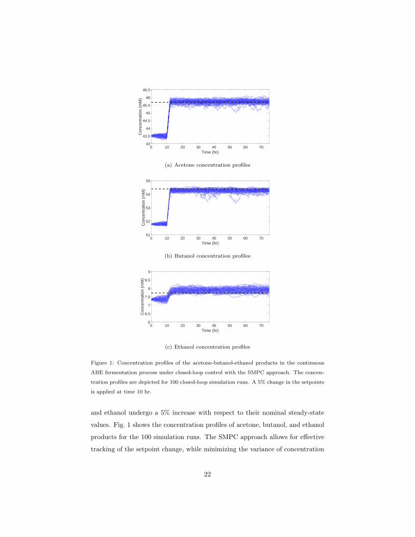
Figure 1: Concentration profiles of the acetone-butanol-ethanol products in the continuous

ABE fermentation process under closed-loop control with the SMPC approach. The concen-

tration profiles are depicted for 100 closed-loop simulation runs. A 5% change in the setpoints

is applied at time 10 hr.

and ethanol undergo a 5% increase with respect to their nominal steady-state

values. Fig. 1 shows the concentration profiles of acetone, butanol, and ethanol

products for the 100 simulation runs. The SMPC approach allows for effective

tracking of the setpoint change, while minimizing the variance of concentration

22

profiles around their respective setpoints. Note that there is a slight offset in

setpoint tracking for the product concentration profiles, in particular for the

ethanol concentration profiles. The offset results from the tradeoff that the

SMPC approach seeks between fulfilling the control objectives and satisfying

the state constraints in the presence of process stochasticity (i.e., state chance

constraints).

Fig. 2 shows the evolution of probability distributions of the acidic species

under SMPC. The state constraints are never violated using SMPC despite al-

lowing for 10% constraint violation. This is attributed to conservative approxi-

mation of the chance constraints using the Cantelli-Chebyshev inequality. Seem-

ingly, the SMPC approach applies a hard bound for acetate and butyrate that is

more conservative than the bounds considered in the state chance constraints.

The ability of SMPC to handle the state constraints in the presence of stochas-

tic uncertainties has been compared to that of a standard MPC controller. The

closed-loop simulation results reveal that the standard MPC controller violates

the state constraints in approximately 20% of simulations. Maintaining these

state constraints is critical to optimal operation of the continuous ABE fermen-

tation, as high concentration of the acidic species can cause the cells to switch

from the desired solventogenesis stage to the undesired acidogenesis stage. The

simulation case study indicates the capability of the SMPC approach in guaran-

teeing the fulfillment of state constraints in the presence of process stochasticity

at the expense of a slight drop in the control performance.

6. Conclusions

A tractable convex optimization program is derived to solve receding-horizon

stochastic model predictive control of linear systems with (possibly) unbounded

stochastic disturbances. Due to the unbounded nature of stochastic distur-

bances, feasibility of the optimization problem cannot always be guaranteed

when chance constraints are included in the formulation. To avoid this issue,

the state chance constraints are softened to ensure the feasibility. The exact

23

(a) Probability distributions of acetate concentration

(b) Probability distributions of butyrate concentration

Figure 2: Evolution of probability distributions of concentration of the acidic species in the

continuous ABE fermentation process under closed-loop control with the SMPC approach.

The probability distributions are obtained based on 100 closed-loop simulation runs, and are

depicted at four different times. The state constraints are always satisfied using the SMPC

approach, whereas the standard MPC controller leads to violation of state constraints in

approximately 20% of the closed-loop simulations (not shown here).

penalty function method is utilized to guarantee the soft-constrained optimiza-

tion yields the same solution as the hard-constrained problem when the latter

is feasible. Building upon the results of [11], it is also shown that the receding-

horizon control policy results in a stochastically stable system by proving the

states satisfy a geometric drift condition outside of a compact set (i.e., the vari-

ance of the states is bounded for all time). Future work includes incorporating

output feedback with measurement noise, as well as reducing the conservatism

introduced by the Cantelli-Chebyshev inequality.

24

Appendix A

This appendix contains the proofs for all Lemmas and Theorems presented

in the paper.

Proof of Lemma 1. Let the ith row of the maximization in (19) be the primal

linear program (LP). The corresponding dual LP is

minzi≥0

k>wzi, s.t.: H>wzi = (HuM)>i ,

where (HuM)i denotes the ith row of HuM; and zi ∈ Ra denotes the dual

variables. By the weak duality of LPs (e.g., see [42]), it is known that the pro-

gram maxϕ(Gw)∈W(HuM)iϕ(Gw) ≤ k>wzi for any zi ≥ 0 satisfying H>wzi =

(HuM)>i . Stacking the dual variables into the matrix Z , [z1, . . . , zsN ] and tak-

ing the transpose of this relationship for all i ∈ Z[1,sN ] results in the inequality

maxϕ(Gw)∈W(HuMϕ(Gw)) ≤ Z>kw for any Z ≥ 0 satisfying Z>Hw = HuM.

Hence, the assertion of the lemma follows from this statement.

Proof of Lemma 2. Let pZ(z) denote the PDF of random variable Z with

mean Z. Define a corresponding zero-mean random variable Y , Z − Z

with PDF pY (y). Consider Pr[Z ≥ Z + a] = Pr[Y ≥ a] =∫∞apY (Y )dz =

E[1[a,∞)(Y )

]. Define the function h(y) , (a+ b)−2(y+ b)2 for any a ∈ R+ and

b ∈ R+. It is evident that 1[a,∞)(y) ≤ h(y), ∀y ∈ R such that E[1[a,∞)(Y )

]≤

E[h(Y )] = (a + b)−2E[(Y + b)2] = (a + b)−2(Var[Y ] + b2). The smallest up-

per bound for Pr[Z ≥ Z + α] is obtained by minimizing the right-hand side

of the latter inequality with respect to b. The solution to this minimization is

b? = Var[Y ]/a. The assertion of Lemma follows by noticing Var[Y ] = Var[Z]

and substituting b? for b into this upper bound of Pr[Z ≥ Z + α].

Proof of Lemma 3. When the inequality a>x ≤ b− δ holds, it is true that

Pr[a>x ≥ b] ≤ Pr[a>x ≥ a>x+ δ]

≤ a>Σxa

a>Σxa+ δ2,

where the second line follows from Lemma 2 for any δ ∈ R+. As the latter

inequality is an upper bound for Pr[a>x ≥ b] ≤ ε, the ICC will be satisfied

25

when

a>Σxa

a>Σxa+ δ2≤ ε.

Rearranging the above inequality results in a>Σxa ≤ εδ2(1 − ε)−1 and, thus,

the proof is complete.

Proof of Theorem 1. The proof consists of four main derivations: (i) a

quadratic expression for the value function, (ii) linear constraints guaranteeing

hard input constraints, (iii) linear and quadratic inequalities for the softened

versions of (22a) and (22b), respectively, and (iv) SOCP formulation of the

soft-constrained version of the optimal control problem (26).

(i) Based on the exact penalty function method, the value function is adapted

as VN (x,M,v) + ρ‖ε‖1. Since by definition ε ≥ 0, ‖ε‖1 = 1>ε can be written

as a linear constraint in the slack variables. Now, consider the value function

(10). Substituting the system dynamics (9) into (10) and assigning x0 = x gives

VN (x,u) = E[‖Ax+ Bu + DGw‖2Q + ‖u‖2R]

= c(x) + E[‖u‖2B>QB+R + 2u>B>Q(Ax+ DGw)],

where c(x) , ‖x‖2A>QA +E[‖w‖2G>D>QDG] since the states x are known. Sub-

stituting the control policy (17) into the above equation and rearranging yields

VN (x,M,v) = c(x) + E[‖Mϕ(Gw) + v‖2S1]

+b>E[Mϕ(Gw) + v] + tr(S2E[(Mϕ(Gw) + v)w>]

).

By assumption, E[ϕ(Gw)] = 0 so that

VN (x,M,v) = c(x) + ‖v‖2S1+ E[‖Mϕ(Gw)‖2S1

]+

b>v + tr(S2MΩ2)

= c(x) + b>v+

‖v‖2S1+ tr(M>S1MΩ1 + S2MΩ2).

As c(x) is independent of the decision variables (M,v,Z, ε), it can be dropped

from the value function. For matrices A, B, and C of appropriate dimensions,

the properties tr(ABC) = tr(CAB) = tr(BCA), vec(ABC) = (C>⊗A)vec(B),

and tr(A>B) = vec(A)>vec(B) hold. Using these, the constraint m = vec(M),

26

and the expressions for ν and Λ, the asserted value function can be obtained

through standard algebraic manipulations. Note that the derived value function

is a convex quadratic function since the matrices S1 ∈ SnuN+ and Λ ∈ SnunxN

2

+

are positive semidefinite.

(ii) From Lemma 1, it is known that the constraints Huv + Z>kw ≤ ku,

Z>Hw = HuM, and Z ≥ 0 exactly represent Pr[Huu ≤ ku

]= 1 for the control

policy (17). The latter constraints are linear in the decision variables (M,v,Z)

and, therefore, convex.

(iii) From the control policy (17) and the assumption E[ϕ(Gw)] = 0, it

can be derived that u = v, Σu = MΩ1M>, and σu,w = MΩ2. Substi-

tuting these definitions into (23) and (24) yields x = Ax0 + Bv and Σx =

BMΩ1M>B> + BMΩ2G

>D> + DGΩ2M>B> + DGΣwG>D>. Constraint

(28h) is obtained by substituting the expression for x into (22a) and introducing

the corresponding slack variables εmi,j . The latter constraint is linear in (v, εmi,j)

and, therefore, convex. Substituting the expression for Σx into (22b) results in

y>i,jΩ1yi,j +y>i,jΩ2G>D>H

[i]>x,j +H

[i]x,jDGΣwG>D>H

[i]>x,j ≤ αkδ2

k(1−αk)−1. It

is evident that y>i,jΩ2G>D>H

[i]>x,j = (y>i,jΩ2G

>D>H[i]>x,j )> since this is a scalar

constraint. Using the latter expression and definitions for q>i,j and ci,j , it can

be stated that y>i,jΩ1yi,j + q>i,jyi,j + ci,j ≤ 0. Constraint (28j) is obtained by

introducing the corresponding slack variables εvi,j . Note that (28j) is linear in

εvi,j and quadratic in M and, therefore, convex since Ω1 ∈ SnxN+ .

(iv) A special case of SOCPs includes convex quadratically constrained

quadratic programs. In the prequel, it was shown that all the constraints in (28)

are linear or quadratic convex expressions. Problem (28) is converted into the

standard SOCP form by introducing a new decision variable g that bounds the

quadratic part of the value function, i.e., v>S1v+m>Λm ≤ g. The value func-

tion in (28) is then replaced by b>v + ν>m + 1>ε+ g. Any convex quadratic

constraint of the form x>Qx + b>x + c ≤ 0 with x ∈ Rn and Q ∈ Sn+ can be

27

formulated as an equivalent SOC constraint,∥∥∥∥∥∥(1 + b>x+ c)/2

Q1/2x

∥∥∥∥∥∥2

≤ (1− b>x− c)/2.

Hence, Problem (28) can be stated in the standard SOCP form by applying the

above result to the new constraint v>S1v + m>Λm ≤ g and (28j).

Proof of Lemma 4. First, from the law of iterated expectations, Ex0 [V (xt)] =

Ex0 [E[V (xt)|xst−1s=1]] = Ex0 [Ext−1 [V (xt)]]. Next, it can be derived from the

premises in Lemma 4 that Ext−1[V (xt)] ≤ λV (xt−1) whenever xt−1 6∈ D and

Ext−1[V (xt)] ≤ b whenever xt−1 ∈ D. Adding these results together gives

Ext−1 [V (xt)] ≤ λV (xt−1)1Rnx\D(xt−1) + b1D(xt−1) for all xt−1 ∈ Rnx . Tak-

ing the expectation over x0 and applying the first result yields Ex0 [V (xt)] ≤

λEx0[V (xt−1)] + bPrx0

[xt−1 ∈ D]. Repeating these steps for Ex0[V (xs)]t−1

s=1

and recursively substituting the derived inequalities into the last inequality re-

sults in

Ex0[V (xt)] ≤ λtV (x0) + b

t−1∑i=0

λiPrx0[xt−1−i ∈ D]

≤ λtV (x0) + b

t−1∑i=0

λi

≤ λtV (x0) + b

∞∑i=0

λi

≤ λtV (x0) + b(1− λ)−1.

Note that Prx0[xt−1−i ∈ D] ≤ 1 and the geometric series expression 1 + λ +

λ2 + · · · = (1− λ)−1, which is convergent for |λ| < 1. The above result implies

that supt∈N0Ex0 [V (xt)] ≤ V (x0) + b(1 − λ)−1 < ∞ is bounded and, thus, the

proof is complete.

Proof of Theorem 2. The proof follows directly from [11]. Recall Holder’s

inequality |a>b| ≤ ‖a‖p‖b‖q for all p, q ∈ N such that p−1 + q−1 = 1, ‖XY ‖p ≤

‖X‖p‖Y ‖p for all p ∈ N, and ‖a‖∞ ≤ ‖a‖1 ≤ n‖a‖∞ and ‖a‖∞ ≤ ‖a‖ ≤√n‖a‖∞, where a, b ∈ Rn, X ∈ Rn×m, and Y ∈ Rm×q.

Since A is assumed Schur stable (see Assumption 1), there exists a matrix

28

P ∈ Snx++ such that A>PA−P ≤ −Inx . Define the measurable function V (x) =

x>Px. From (34), it can be written that

Ext [x>t+1Pxt+1] = x>t A

>PAxt + 2x>t A>PBκsN (xt)

+ κsN (xt)>B>PBκsN (xt) + tr(G>PGΣw).

As the hard input constraints (2) are assumed to be compact, there exists some

set U1 , u ∈ Rnu | ‖u‖1 ≤ Ub and Ub ∈ R+ such that U ⊆ U1. Since

κsN (x) ∈ U must hold in PsN (x), ‖κsN (x)‖1 ≤ Ub for all x ∈ Rnx . An upper bound

can now be derived for the second and third terms in the above expression for

Ext [x>t+1Pxt+1], i.e.,

2x>t A>PBκsN (xt) = 2(B>PAxt)

>κsN (xt)

≤ 2‖B>PAxt‖∞‖κsN (xt)‖1≤ 2‖B>PA‖∞Ub‖xt‖∞

κsN (xt)>B>PBκsN (xt) = (B>PBκsN (xt))

>κsN (xt)

≤ ‖B>PBκsN (xt)‖∞‖κsN (xt)‖1≤ ‖B>PB‖∞‖κsN (xt)‖21≤ ‖B>PB‖∞U2

b .

Define c1 = ‖B>PA‖∞Ub and c2 = ‖B>PB‖∞U2b + tr(G>PGΣw) such that

Ext [x>t+1Pxt+1] ≤ x>t A>PAxt+2c1‖xt‖∞+c2 ≤ x>t Pxt−‖xt‖2+2c1‖xt‖∞+c2.

By definition c1 ∈ R++ and c2 ∈ R++ such that 2c1‖xt‖∞ + c2 ≤ θ‖xt‖2∞ for

some θ ∈ R++. The latter expression can be rewritten as −θ(‖xt‖∞ − c1θ )2 +

c2 +c21θ ≤ 0 such that 1

θ (c1 +√c21 + c2θ) ≤ ‖xt‖∞. Let r = 1

θ (c1 +√c21 + c2θ)

and define D , x ∈ Rnx | ‖x‖∞ ≤ r. For all xt 6∈ D, the definition of

D results in 2c1‖xt‖∞ + c2 ≤ θ‖xt‖2∞ ≤ θ‖xt‖2 such that Ext[x>t+1Pxt+1] ≤

x>t Pxt−(1−θ)‖xt‖2. As P ∈ Snx++, it is known that x>t Pxt ≤ λmax(P )‖xt‖2 with

λmax(P ) > 0 yielding Ext[x>t+1Pxt+1] ≤ (1− 1−θ

λmax(P ) )x>t Pxt for all ‖xt‖∞ 6∈ D.

For the latter expression to represent a decay outside of D, the constant θ must

satisfy 1−λmax(P ) < θ < 1. Since λmax(P ) > 0, there exists at least one θ that

satisfies these inequalities.

29

Hence, the premises of Lemma 4 are satisfied with the following definitions:

V (x) , x>Px, D , x ∈ Rnx | ‖x‖∞ ≤ r, b , supxt∈D Ext[x>t+1Pxt+1],

and λ , (1 − 1−θλmax(P ) ) for any θ ∈ [1 − λmax(P ), 1]. It directly follows that

Ex0[x>t Pxt]t∈N0

is bounded for all x0 ∈ Rnx . Since λmin(P )‖xt‖2 ≤ x>t Pxt,

the assertion holds and the proof is complete.

Appendix B

This appendix contains the description of the state-space model of the con-

tinuous acetone-butanol-ethanol fermentation process used in Section 5. The

state vector is defined as

x = [CAC CA CEn CAaC CAa CBC CB

CAn CBn CAd CCf CAh]>,

where C denotes concentration (mM) of AC = Acetyl-CoA, A = Acetate, En =

Ethanol, AaC = Acetoacetate-CoA, Aa = Acetoacetate, BC = Butyryl-CoA, B

= Butyrate, An = Acetone, Bn = Butanol, Ad = adc, Cf = ctfA/B, and Ah =

adhE (see [17]). The input vector is defined as

u = [D G0]>,

where D is the dilution rate (hr−1); and G0 is the inlet glucose concentration(mM). The system matrices are given by

A =

0.888 0.017 0 0.143 0 0 −0.002 0 0 0 0.017 −0.002

−0.001 0.969 0 −0.151 0 0 0.002 0 0 0 −0.018 −0.002

0.083 0.001 0.988 0.007 0 0 0 0 0 0 0.001 0.002

0.015 −0.017 0 0.716 0 0 −0.018 0 0 0 −0.032 0

0 0 0 0 0 0 0 0 0 0 0 0

0 0 0 0 0 0 0 0 0 0 0 0

−0.001 0.001 0 −0.122 0 0 0.968 0 0 0 −0.014 0

0.003 0.017 0 0.273 0.988 0 0.018 0.988 0 0 0.0321 0

0 0 0 0 0 0 0 0 0 0.988 0 0

0 0 0 0 0 0 0 0 0 0 0.988 0

0 0 0 0 0 0 0 0 0 0 0 0.988

,

B>

= −

0.220 2.39 1.23 0.157 0 0 1.86 7.33 8.63 0.242 2.34 6.29

0 0 0 0 0 0 0 0 0 0 0 0

,

and G = diag(1, 1, 1, 1, 1, 1, 1, 1, 1, 1, 1, 1).

30

References

[1] A. Bemporad, M. Morari, Robust model predictive control: A survey, in:

Robustness in identification and control, Springer, London, 1999, pp. 207–

226.

[2] D. Limon, T. Alamo, D. M. Raimondo, J. M. Bravo, D. M. de la Pena,

A. Ferramosca, E. F. Camacho, Input-to-state stability: A unifying frame-

work for robust model predictive control, in: Nonlinear Model Predictive

Control, Springer-Verlag, Berlin, 2009, pp. 1–26.

[3] D. Q. Mayne, Model predictive control: Recent developments and future

promise, Automatica 50 (2014) 2967–2986.

[4] A. Mesbah, Stochastic model predictive control: A review, Submitted to

IEEE Control Systems Magazine.

[5] M. Cannon, B. Kouvaritakis, X. Wu, Probabilistic constrained MPC for

multiplicative and additive stochastic uncertainty, IEEE Transactions on

Automatic Control 54 (2009) 1626–1632.

[6] M. Cannon, B. Kouvaritakis, S. V. Rakovic, Q. Cheng, Stochastic tubes in

model predictive control with probabilistic constraints, IEEE Transactions

on Automatic Control 56 (2011) 194–200.

[7] B. Kouvaritakis, M. Cannon, Developments in robust and stochastic pre-

dictive control in the presence of uncertainty, ASCE-ASME Journal of Risk

and Uncertainty in Engineering Systems, Part B: Mechanical Engineering

In Press.

[8] J. M. Lee, J. H. Lee, Approximate dynamic programming strategies and

their applicability for process control: A review and future directions, In-

ternational Journal of Control Automation and Systems 2 (2004) 263–278.

[9] M. Farina, L. Giulioni, L. Magni, R. Scattolini, An approach to output-

feedback MPC of stochastic linear discrete-time systems, Automatica 55

(2015) 140–149.

31

[10] F. Oldewurtel, C. N. Jones, M. Morari, A tractable approximation of chance

constrained stochastic MPC based on affine disturbance feedback, in: Pro-

ceedings of the 47th IEEE Conference on Decision and Control, Cancun,

2008, pp. 4731–4736.

[11] P. Hokayem, D. Chatterjee, J. Lygeros, On stochastic receding horizon

control with bounded control inputs, in: Proceedings of the 48th IEEE

Conference on Decision and Control, Shanghai, 2009, pp. 6359–6364.

[12] P. Hokayem, E. Cinquemani, D. Chatterjee, F. Ramponi, J. Lygeros,

Stochastic receding horizon control with output feedback and bounded con-

trols, Automatica 48 (2012) 77–88.

[13] J. A. Paulson, S. Streif, A. Mesbah, Stability for receding-horizon stochastic

model predictive control, in: Proceedings of the American Control Confer-

ence, Chicago, 2015, p. In Press.

[14] I. Batina, Model Predictive Control for Stochastic Systems by Randomized

Algorithms, Ph.D. Thesis, Eindhoven University of Technology, 2004.

[15] L. Blackmore, M. Ono, A. Bektassov, B. C. Williams, A probabilistic

particle-control approximation of chance-constrained stochastic predictive

control, IEEE Transactions on Robotics 26 (2010) 502–517.

[16] G. Calafiore, L. Fagiano, Robust model predictive control via scenario op-

timization, IEEE Transactions on Automatic Control 58 (2013) 219–224.

[17] S. Haus, S. Jabbari, T. Millat, H. Janssen, R. J. Fischer, H. Bahl, J. R.

King, O. Wolkenhauer, A systems biology approach to investigate the ef-

fect of pH-induced gene regulation on solvent production by Clostridium

acetobutylicum in continuous culture, BMC Systems Biology 5 (10).

[18] J. Lofberg, Minimax approaches to robust model predictive control, Ph.D.

Thesis, Linkoping University, 2003.

32

[19] A. Ben-Tal, A. Goryashko, E. Guslitzer, A. Nemirovski, Adjustable ro-

bust solutions of uncertain linear programs, Mathematical Programming

99 (2004) 351–376.

[20] P. J. Goulart, E. C. Kerrigan, J. M. Maciejowski, Optimization over state

feedback policies for robust control with constraints, Automatica 42 (2006)

523–533.

[21] D. Chatterjee, P. Hokayem, J. Lygeros, Stochastic receding horizon control

with bounded control inputs: A vector space approach, IEEE Transactions

on Automatic Control 56 (2011) 2704–2710.

[22] A. Marshall, I. Olkin, Inequalities: Theory of Majorization and its Appli-

cations, Academic Press, New York, 1979.

[23] M. Athans, The role and use of the stochastic linear-quadratic-Gaussian

problem in control system design, IEEE Transactions on Automatic Control

16 (1971) 529–552.

[24] J. A. Primbs, C. H. Sung, Stochastic receding horizon control of constrained

linear systems with state and control multiplicative noise, IEEE Transac-

tions on Automatic Control 54 (2009) 221–230.

[25] E. Cinquemani, M. Agarwal, D. Chatterjee, , J. Lygeros, Convexity and

convex approximations of discrete-time stochastic control problems with

constraints, Automatica 47 (2011) 2082–2087.

[26] C. Wang, C. J. Ong, M. Sim, Convergence properties of constrained linear

system under MPC control law using affine disturbance feedback, Auto-

matica 45 (2009) 1715–1720.

[27] E. C. Kerrigan, J. M. Maciejowski, Soft constraints and exact penalty func-

tions in model predictive control, in: Control 2000 Conference, Cambridge,

2000.

33

[28] M. Hovd, R. D. Braatz, Handling state and output constraints in MPC

using time-dependent weights, in: Proceedings of the American Control

Conference, Arlington, VA, 2001, pp. 2418–2423.

[29] M. N. Zeilinger, C. N. Jones, M. Morari, Robust stability properties of

soft constrained MPC, in: Proceedings of the 49th IEEE Conference on

Decision and Control, Atlanta, 2010, pp. 5276–5282.

[30] M. Hovd, Multi-level programming for designing penalty functions for MPC

controllers, in: Proceedings of the 18th IFAC World Congress, Milan, 2011,

pp. 6098–6103.

[31] N. de Oliveira, L. T. Biegler, Constraint handing and stability properties

of model predictive control, AIChE Journal 40 (1994) 1138–1155.

[32] S. P. Meyn, R. L. Tweedie, Markov Chains and Stochastic Stabiliy, Cam-

bridge University Press, Cambridge, 2009.

[33] D. Chatterjee, J. Lygeros, On stability and performance of stochastic pre-

dictive control techniques, IEEE Transactions on Automatic Control 60

(2015) 509–514.

[34] Y. S. Jang, A. Malaviya, C. Cho, J. Lee, S. Y. Lee, Butanol production

from renewable biomass by clostridia, Bioresource Technology 123 (2012)

653–663.

[35] N. Qureshi, T. C. Ezeji, Butanol, ’a superior biofuel’ production from agri-

cultural residues (renewable biomass): Recent progress in technology, Bio-

fuels, Bioproducts, and Biorefining 2 (2008) 319–330.

[36] V. Garcıa, J. Pakkila, H. Ojamo, E. Muurinen, R. L. Keiski, Challenges

in biobutanol production: How to improve the efficiency?, Renewable and

Sustainable Energy Reviews 15 (2011) 964–980.

[37] S. M. Lee, M. O. Cho, C. H. Park, Y. C. Chung, J. H. Kim, B. I. Sang,

Y. Um, Continuous butanol production using suspended and immobilized

34

Clostridium beijerinckii NCIMB 8052 with supplementary butyrate, En-

ergy and Fuels 22 (2008) 3459–3464.

[38] J. Zheng, Y. Tashiro, T. Yoshida, M. Gao, Q. Wang, K. Sonomoto, Con-

tinuous butanol fermentation from xylose with high cell density by cell

recyling system, Bioresource Technology 129 (2013) 360–365.

[39] S. Bankar, S. Survase, R. Singhal, T. Granstrom, Continuous two stage

acetone-butanol-ethanol fermentation with integrated solvent removal us-

ing Clostridium acetobutylicum B 5313, Bioresource Technology 106 (2012)

110–116.

[40] M. Grant, S. Boyd, CVX: Matlab software for disciplined convex program-

ming, version 2.1, http://cvxr.com/cvx (Last Visited March 2014).

[41] M. Grant, S. Boyd, Graph implementations for nonsmooth convex pro-

grams, in: V. Blondel, S. Boyd, H. Kimura (Eds.), Recent Advances in

Learning and Control, Springer-Verlag, London, 2008, pp. 95–110.

[42] S. Boyd, L. Vandenberghe, Convex Optimization, Cambridge University

Press, Cambridge, 2004.

35